Application of Dynamic Traffic Assignment (DTA) Model to Evaluate Network Traffic Impact during Bridge Closure - A Case Study in Edmonton, Alberta

Peter Xin, P.Eng. Senior Transportation Engineer

Policy Implementation & Evaluation Transportation Planning, City of Edmonton

Arun Bhowmick, P.Eng.

Senior Transportation Engineer Policy Implementation & Evaluation

Transportation Planning, City of Edmonton

Ido Juran, Ph.D. Senior Analyst

INRO Solutions, Ottawa

Paper Prepared for presentation at the Session “Best Practices in Urban Transportation Planning”

Of the 2014 Conference of the Transportation Association of Canada

Montreal, Quebec

1

[Abstract] The application of macroscopic travel demand models to quantify traffic operational performance measures, such as delay, queues, level of service, and corridor travel time has some significant limitations. Due to the lack of temporal variation of traffic flow in Static Traffic Assignment (STA) and allowance of demand over capacity in macroscopic travel demand models, the validity and reliability of traffic diversion estimate from major road/bridge closures are often subject to question. Dynamic Traffic Assignment (DTA), on the other hand, is a new and evolving technique which is sensitive to time dependent congestion phenomenon and thus can properly estimate traffic diversion to alternate routes during temporal/spatial traffic flow shifts induced by network supply or traffic demand changes. In summer 2013, the City of Edmonton closed the Stony Plain Road Bridge crossing over Groat Road for four months as part of its roadway rehabilitation program. In order to estimate traffic diversion and evaluate network traffic impacts during the construction period, a DTA model was developed using the Dynameq program. Unlike most models where both the calibration and validation data is collected from the same traffic condition, this model utilized the bridge open (pre-construction) traffic data for model calibration, and the bridge closure (during-construction) data for model validation. Additionally, since traffic demand before and during the short-term bridge closure will likely be the same, the assessment of the model forecasting capability can be considered more credible. This paper presents the DTA model development and traffic impact evaluation process, which covers data collection and analysis, traffic origin-destination demand adjustment, the DTA model network preparation, as well as model calibration and validation using the traffic conditions observed before and during the Stony Plain Road Bridge closure. It is expected that the findings and lessons learned from this study will provide practitioners the understandings and benefits of a DTA model in the application of traffic operational analysis. Recommendations on how to apply a calibrated DTA model to a short-term network supply change are also highlighted. 1. Introduction 1.1 Background Overview Recently, the need for detailed operational analysis in transportation planning projects is becoming more evident in order to quantify traffic performance measures, such as travel time, queue, delay, level of service, etc. In a traditional approach, travel demand models are used to forecast link and intersection volumes under various assumptions of future transportation network and/or land uses. The forecasted traffic data is then imported into traffic operational models to conduct detailed operational analysis. Due to the use of static traffic assignment (STA), travel time and cost measures in macroscopic travel demand models are not time sensitive, and link based volume-delay functions (VDF)

2

cannot appropriately address congestion spillback and traffic lane utilization. In comparison, the most common route choice behaviour for dynamic traffic assignment (DTA) in the context of transportation planning applications is dynamic user equilibrium (DUE) route-choice methodology. Thus DTA intends to represent the interaction among travel choices, traffic flows, and time and cost measures in a temporally coherent manner (1). One of the challenges of analyzing DTA model results in forecast scenarios is to define the measure of success. The obvious question here is how credible the DTA results are. To assess this, a rigorous calibration and validation for the base model must be conducted. In transportation planning, most models are calibrated and validated using the data set observed from the same traffic condition. Using traffic data sets observed at different traffic conditions, one for model calibration and one for validation will increase the confidence level of the model credibility assessment. As it is generally accepted that trip makers’ travel behavior does not change much during a short-term roadway construction, the traffic demand during the construction period can be assumed to be the same as pre-construction. Therefore, a short-term construction detour project would be ideal to evaluate the credibility of the DTA model without considering demand difference between base and forecast scenarios. The pre- and during-construction traffic data could then be used for model calibration and validation, respectively. In order to undertake roadway rehabilitation, the City of Edmonton closed the Stony Plain Road Bridge over Groat Road for four months during the summer of 2013. With the availability of both the bridge open (pre-construction) and closure (during-construction) traffic data, this project was chosen for a case study to evaluate the credibility and benefits of DTA models in transportation planning projects. Based on the study findings, several recommendations on how to apply a calibrated DTA model to a very short-term network supply change (e.g. construction detour projects) were proposed. 1.2 Project Highlight Stony Plain Road (SPR) is one of major east-west arterials in the City of Edmonton. Carrying about 20,000 to 30,000 vehicles per day in 2012, it handles a large portion of peak hour commuting trips between the Downtown and west-end residential communities. Within the City, SPR aligns with 104 Avenue at 124 Street to the east, merges with 102 Avenue at 142 Street, and extends to the City west limit as Highway 16A. Between 124 Street and 170 Street, SPR is mainly a 4-lane undivided arterial. At the bridge crossing over Groat Road, the westbound traffic varied up to 1,800 vehicles during the fall weekday PM Peak hour. Figure 1 shows the alignment of SPR and the bridge location. It was expected that during the bridge closure, traffic over the bridge would divert to other parallel routes including 102 Avenue, 107 Avenue and 111 Avenue. As a result, significant traffic impact would be observed on these corridors near Groat Road. The SPR DTA model was expected to reproduce the traffic diversion pattern and network traffic impact during the bridge closure. Edmonton, like other major Canadian cities, has the highest vehicle traffic demand in the fall weekday PM Peak period, thus this DTA model development focused on vehicle traffic in two hours of PM Peak period (4:00 – 6:00 PM). Other modes of traffic including cyclists and pedestrians are not included.

3

Selection of DTA Model Boundary One of the major advantages of a DTA model is that it can capture the localized traffic impacts due to network changes. However, the boundary of the localized traffic impacts is critical and must be determined carefully so that the proper extent of the impacts is adequately covered. In order to determine the extent of the traffic impacts during the SPR Bridge closure, a traffic reassignment was performed in the 2010 Edmonton Region Travel Model (RTM) with a revised roadway network representing the bridge closure. Based on the traffic diversion pattern in the RTM, together with our local experience and engineering judgment, the model boundary for this study was identified. As shown in Figure 1, the study area boundaries are:

118 Avenue and Kingsway Avenue to the north

95 Avenue and the North Saskatchewan River to the south

170 Street to the west, and

97 Street, 103a Avenue and the North Saskatchewan River to the east 1.3 Study Approach This study mainly covers the following three topics:

Development of the SPR DTA base model using the bridge open traffic data

Validation of the model using the bridge closure traffic data

Network traffic impact analysis using DTA model results 2. DTA Base Model Development Major tasks accomplished for the SPR Bridge open (pre-construction) DTA model development include data collection, sub area model and demand adjustment, DTA model network supply and demand preparation, and model calibration and validation tasks. 2.1 Data Collection Primarily, three types of data including network supply, traffic demand and model calibration/validation data, are required for model development. Network supply and traffic demand data are the model inputs, while model calibration and validation data are used for model output comparisons. 2.1.1 Network Supply Data Transportation Network Geometry The transportation network geometry includes road classification, link length, number of lanes, lane width, free flow speeds, bus routes and stop locations, as well as intersection configurations. Major resources for the network geometry data include the City Synchro files, GIS shape files, posted speed limit map and the open Google aerial photos.

4

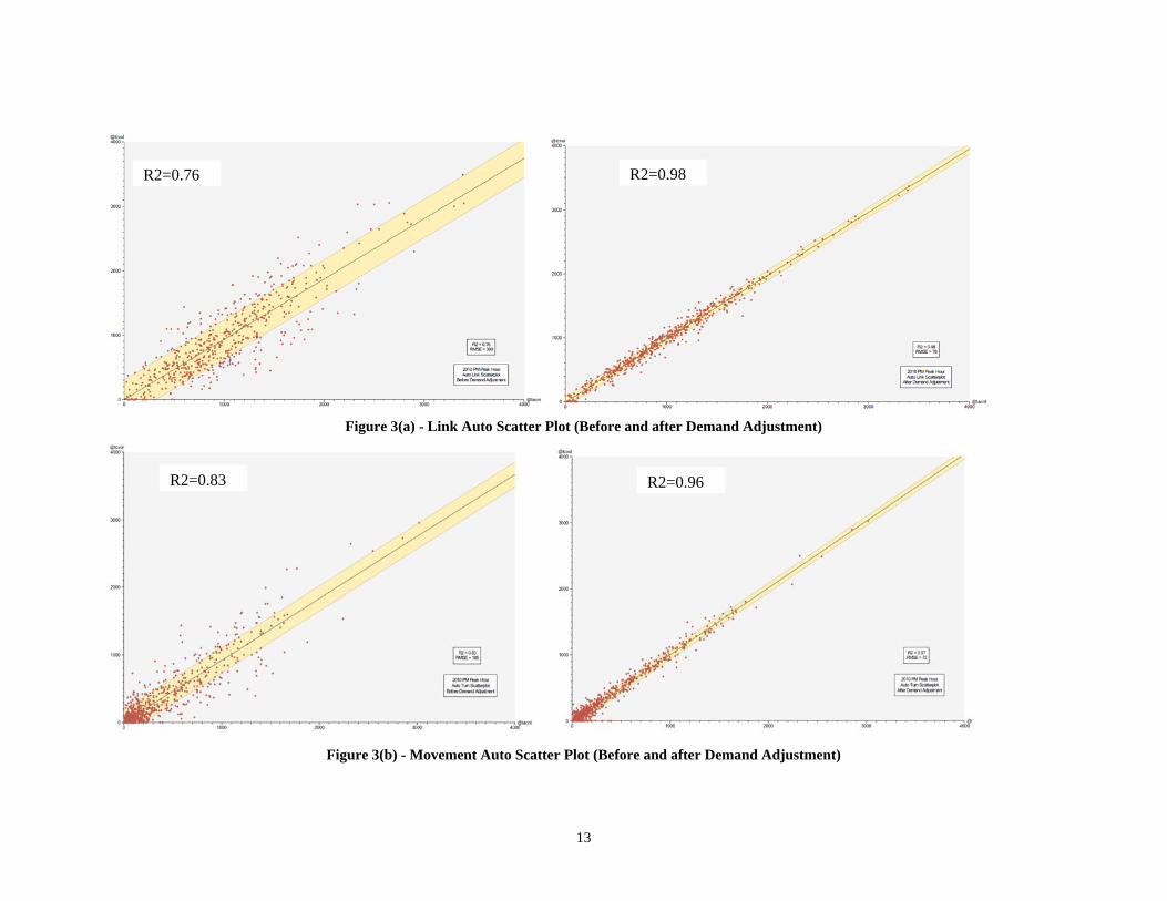
Intersection Control Signal plans, including phasing and timing, are essential for DTA modeling. In addition, the locations of unsignalized intersections and priority rules are also required. To obtain this type of data, the City existing PM Peak Synchro files and Google aerial photos were reviewed and compiled. 2.1.2 Traffic Demand The City RTM was used to forecast auto and truck vehicle demand in the study area. For transit demand, the 2012 transit scheduling handbook was used to estimate transit buses in the study area. 2.1.3 Model Calibration/Validation Data For this study, traffic counts at 73 signalized intersections and 7 bridges crossing the North Saskatchewan River, as well as travel times of 7 arterial corridors either across or parallel to Groat Road, were collected. The locations of the traffic counts and travel time corridors are shown in Figure 2. Gathering the traffic data for this study was a significant undertaking. For the SPR Bridge open scenario, the historical (collected between 2007 and 2012) auto and truck volumes at 15 minute interval were utilized. For the bridge closure scenario, the City Traffic Monitoring Group conducted similar traffic volume counts between July and August 2013. Travel times along the 7 arterial roadway corridors were also gathered by the Traffic Monitoring Group for both the bridge open and closure scenarios. 2.2 Sub Area Model and Demand Adjustment Estimating spatial and temporal distribution of traffic demand is critical for a DTA model. One common approach is to extract a sub area model from a regional demand model, and then perform demand adjustment, if necessary. It is to be noted that network coding, model calibration parameters and traffic count input discrepancies should be carefully checked before conducting demand adjustment. Using EMME’s Subarea module, a sub area model containing car and truck modes was extracted from the City’s 2010 RTM. As part of the subarea model development, a thorough network review was completed for roadway and zone system updates including link length, number of lanes, volume delay functions (VDF) and posted speeds, as well as zone access locations and splits, if applicable. Once the network was finished, an iterative process of demand adjustment was conducted to improve the degree of correlation between the model volumes and traffic counts. Figures 3(a) and 3(b) are the PM Peak hour (4:30 to 5:30 PM) model Auto volumes and counts scatter plots before and after the demand adjustment. The closer the two data sets agree, the more the scatters tend to concentrate in the vicinity of the identity line. After demand adjustment, the R2 increased from 0.76 to 0.98 and 0.83 to 0.96 for link and intersection movement traffic, respectively. It is mentioned earlier that the model results and network impact were evaluated based on a complete traffic simulation analysis of a two hour PM Peak period from 4:00 PM to 6:00 PM. In addition to this two hour traffic demand, 30 minutes (3:30-4:00 PM) seeding and 30 minutes

5

(6:00-6:30 PM) cooling durations were also considered as part of the model run. The seeding duration was considered to load the traffic into the network and the cooling duration was considered to clear the loaded traffic off the network. These 30 minute buffer periods were selected based on the longest travel time across the study area for a given O-D pair. The demand between 3:30 to 4:30 PM and 5:30 to 6:30 PM were then estimated using the above demand adjustment procedure. 2.3 DTA Model Network and Demand Preparation The following 5 steps were considered to prepare the Stony Plain Road DTA model network and demand. Step 1: Develop a Complete Synchro Network The City of Edmonton maintains Synchro files for signalized intersections by corridors. All the corridor Synchro files in the study area were compiled and merged to form an initial network. Based on Google aerial photos, the initial Synchro network was then updated to include all arterial and collector roadways, as well as some local roads essential for zone connections. All the unsignalized intersections in the network were updated to represent appropriate priority rules. Step 2: Import Synchro File to Dynameq Using Dynameq’s Synchro Import function, a coarse DTA network, including intersection control setting and signal timing plans, was created. Link traffic flow parameters (e.g. free flow speeds, effective length factor and response time factor) and node turn capacity parameters (e.g. speed, protective and permissive capacities, follow up times) were either taken from Synchro files or calculated by Dynameq based on Synchro import. Dynameq permits the two vehicle type parameters (effective length and response time factors) to vary from one link to another by providing a link-specific multiplication factor for each one. These two parameters reflect driver behavior and can change depending on the physical characteristics of a link (2). Extensive effort had been taken to review and fine tune the coarse Dynameq network, including geometry refinement, signal timing update for pedestrian actuated signals at two-way stop controlled intersections, critical gap time adjustment for yield controlled intersections and priority rules update for merge and diverge locations. Step 3: Add Traffic Zone System and Import Traffic Demand Since a Synchro network does not have zone centroids and connectors, the DTA network imported from Synchro was built without a traffic zone system. Therefore, the same zone system in the EMME sub area model and corresponding zone connectors had to be added. With the addition of the zone system, the three hour PM Peak demand estimated in the EMME sub area model was then imported into the DTA model. Step 4: Code Transit Network The City 2010 transit scheduling book and transit stop GIS file were used to code transit routes and dwell times. For this model, 60 second dwell time was coded for transit centres and downtown transit stops. For other stops, 15 second dwell time was used.

6

To define the proportion of vehicle components, effective length and response time for each class of vehicle (auto, truck and transit), the detailed vehicle classification of existing traffic counts was analyzed. Step 5: Import Traffic Counts to DTA The last step before calibrating the DTA model was to import traffic counts. Since the DTA model has a finer node and link network system (compared with EMME sub area model), a Python script was written to import 15 minute interval intersection turning movement auto and truck counts for the PM period between 15:30 and 18:30 pm. The inbound and outbound link counts were then aggregated using the turning movement counts. The established SPR DTA model has 138 traffic zones, 4085 links, 140 transit lines and 1624 nodes. Among the nodes, there are 261 signalized intersections, 32 all-way stop controlled, and 415 two-way stopped controlled intersections. 2.4 Model Calibration An iterative process was adopted to calibrate the SPR DTA base model, which included adjusting model network connections and capacity parameters, and executing the DTA model until traffic assignment was converged and the model output data matched reasonably well with observed data. A flow chart of model calibration and validation is shown in Figure 4. Considering that more than 95% of traffic in the study area belongs to auto, and transit lines have fixed alignments, the model calibration and validation for this study focused on the auto mode only. 2.4.1 Network Debugging In Dynameq, convergence is measured by comparing the average travel time with the shortest travel time for each O-D pair and for each assignment interval (2). Without a good convergence, the output from a DTA model will be fluctuating, and validation of model results becomes futile. As an example below (Figure 5), the first model run was deemed not converged, and the mean value of relative gap was more than 14% after 200 iterations. After a careful network debugging and zone connections adjustment, it appeared the restricted HCM capacities (in Synchro), which are typically used in static models, were not suitable to a simulation based DTA model, such as Dynameq. Capacities in Dynameq are not an exogenous model input but rather an endogenous variable continuously modified throughout the simulation based on vehicle interactions. As such, the following adjustments were made to the original value that was calculated to produce Synchro turn capacities:

• Turning movement follow-up (gap) time: 3 seconds if they are longer than 3 seconds from the Synchro import

• Movement speeds: 25 km/h for right turn movements, 30 km/h for left turn movements and link free flow speeds for through movements

• Link response time factor: 1.0

7

2.4.2 Route Choice Calibration With the above modifications, the model assignment converged quite well with a mean relative gap value of 2.5% after 60 iterations. However, path analysis for a number of O-D pairs indicated that short cutting traffic using internal collector/local roadways resulted in model volumes much lower than observed counts at a few signalized intersections. Therefore, additional turn penalties (30 seconds for all left turn movements and 10 seconds for all right turn movements) were incorporated as ‘generalized cost’ in the model. 2.4.3 Demand Refinement After network debugging and route choice analysis, there were still some locations with model volumes unreasonably higher or lower than observed counts. Therefore, demand input was refined for several O-D pairs based on select link/turn analysis results. Figure 6 shows the final model convergence plot. It converged very well with a mean convergence value of 1.6% at 60 runs. Auto mode scatter plots between model volumes and observed counts at the intersection turning movement level are shown in Figures 7(a) and 7(b) for the PM Peak hours between 4:00 to 5:00 pm and 5:00 to 6:00 pm, respectively. They indicate that the model was well calibrated, with R2 of 0.92 and slope close to 1 for the both peak hours. Travel times along the 7 surveyed corridors were also extracted from the model and compared with the observed travel times. Figure 8 indicates that overall the DTA model travel times were quite comparable to the field travel times. 2.5 Model Validation In order to validate and further assess the DTA model forecasting reliability, the calibrated base model was used to validate the Stony Plain Road Bridge closure (during-construction) scenario. As such, the network supply and intersection control data, including roadway and transit network as well as intersection signal timings, were updated as per the City construction detour and signal timing re-optimization plans. Given that the bridge closure only lasted for 4 months, it was assumed that the trip makers had not yet reacted to the closure by adjusted their travel patterns. Therefore, the traffic demand under the bridge open scenario was loaded on the revised network to form the bridge closure DTA model. 2.5.1 Model Results Analysis With the assignment of same demand in the bridge open scenario, it was expected that the traffic in the network will be more congested and required longer time to achieve equilibrium status. For this DTA model, it took 160 iterations to converge with a mean relative gap value of 2.3%. The auto movement volumes regression analysis indicates that the DTA model projection is acceptable, with R2 of 0.89 and 0.87 for the two peak hours. The travel times comparison plot (Figure 9) shows that the model travel times were quite comparable with the observed corridor times. However, volume differences at the locations along or near Groat Road were quite high. For example, the westbound traffic at the 107 Avenue Bridge over Groat Road was overestimated by

8

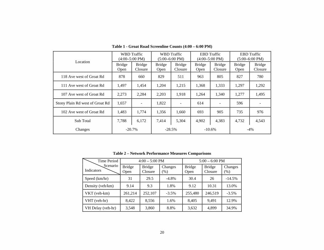
800 vehicles during 5:00 to 6:00 PM. Based on a demand review of the screenline counts of Groat Road, combined with analysis of screenline capacity, it was revealed that the traffic demand estimated for the bridge open scenario was not appropriate for the bridge closure. 2.5.2 Travel Demand Exploration In order to assess the accuracy of the demand assumption for the bridge closure, Groat Road was chosen as a screenline to compare traffic counts before and during the bridge closure. As shown in Table 1, a more than 20% decrease of westbound traffic across Groat Road was observed when the bridge was closed for construction. There are likely three reasons contributing to the demand inconsistency:

Seasonal Variation: It was noticed that traffic counts were collected in different seasons and years. The majority of the counts were collected in the Spring or Fall between 2007 and 2011 for the bridge open scenario, while all the bridge closure counts were collected in summer 2013. Typically, the traffic counts on the Edmonton’s streets are lower in summer, due to school closure and out-of-town vacation trips. This could be the major reason that demand within the study area was different during the bridge open and closure scenarios.

Shift in Demand: With the bridge closure, traffic along Stony Plain Road was expected to use other parallel corridors, which would result in more congestion and lower speeds along these corridors, particularly for the westbound traffic on 102 Avenue and 107 Avenue in the PM Peak. Trip makers thus may consider different travel choices (e.g. alternative modes, and/or different time of departure) to avoid delay. As a result, traffic demand across Groat Road in the PM Peak period could decrease.

Model Boundary: It was observed that some traffic shifted to use travel paths outside the study boundary during the bridge closure (e.g. traffic shifted to use Groat Road Bridge and Quesnell Bridge at Whitemud Drive). A bigger study area including Quesnell Bridge would benefit to capture all route changes.

Based on the bridge closure traffic counts, the travel demand crossing Groat Road was adjusted for a quick scenario test. The revised model run results were improved with slight higher R2 values, and the model volumes within the vicinity of Groat Road corridor were comparable with the traffic counts. However, given that traffic counts will be not available during scenario tests for typical planning projects, it is not realistic to adjust demand based on counts for forecast scenarios. Therefore, the network impact analysis under the next section was completed using the unadjusted demand for the bridge closure scenario. 3. Network Impact Analysis A number of traffic operational measures can be quantified by DTA models. To assess the network traffic impact for this study, the average hourly traffic flow, travel delay, as well as 15 minute queue lengths at the bridge open and closure scenarios were extracted for comparison. Figure 10 illustrates traffic flow between 5:00 and 6:00 pm. As anticipated, traffic volumes along Stony Plain Road mainly shifted to 102 Avenue and 107 Avenue across Groat Road when the bridge was closed. From the travel delay plot (Figure 11), it was observed that traffic along 107 Avenue across Groat Road, as well as Jasper Avenue & 124 Street, would be very congested with significant delay during the bridge closure.

9

Another major performance measure is queue length by lanes. Figure 12 illustrates queue plots between 5:20 and 5:25 PM. During the bridge closure for construction, queues would increase dramatically for the following movements:

Westbound traffic on 107 Avenue between 124 Street and 142 Street

Westbound and Northbound traffic at Groat Road and 111 Avenue

Westbound traffic on Jasper Avenue at 124 Street Table 2 summarizes network wide traffic performance measures. Overall, traffic congestion will be worse for the bridge closure scenario, particularly for the peak hour from 5:00 to 6:00 PM. For example, the average speed would decrease by 5% and 15% from 4:00 to 5:00 PM and 5:00 to 6:00 PM, respectively. Total vehicle delay hours would increase by 8.8% and 35% for the two peak hours, respectively. 4. Conclusions 4.1 Study Findings The Stony Plain Road over Groat Road Bridge Rehabilitation project was chosen as a DTA model application case study. Several conclusions and findings obtained from the model development and application are summarized below.

This case study used two sets of traffic counts and travel time data observed during a short-term period construction detour project, the pre-construction (bridge open) data for the DTA model calibration and the during-construction (bridge closure) data for the model validation. Availability of the pre- and during-construction data provided a better and more rigorous evaluation for the credibility of DTA model results.

Demand adjustment is an effective tool to improve model forecasting reliability. However, demand adjustment should be the last step after checking network coding, traffic count input, and testing model calibration parameters.

Synchro files have detailed network configuration and intersection control data. Typically importing Synchro files to Dynameq for a DTA model preparation is a good starting point. However, since Synchro uses the restricted HCM capacities which are typically used in static models, it is not suitable to use these capacities in a simulation based DTA model such as Dynameq. Capacities in Dynameq are not an exogenous model input but rather an endogenous variable continuously modified throughout the simulation based on vehicles interactions. As a result, the capacity parameters estimated based on Synchro import should be carefully analyzed.

Consistency of traffic counts and travel times is very important for model calibration and validation. Collecting counts and travel times at the same season and year is strongly recommended. For congested network changes and/or longer term forecast scenarios, regional travel models or travel surveys maybe required to analyze mode, time of departure and/or destination choices changes.

The analysis of the Groat Road screenline counts indicates that assessment of the applicability of the base model demand to a forecast scenario should include the analysis of screenline counts if available, and screenline capacities.

10

A DTA model boundary should capture all route changes due to network or land use changes. One typical approach to determine a study area is to analyze traffic reassignment results from a regional demand model run with a reduced capacity network.

To minimize short cutting in DTA models, additional turn penalties as “generalized cost” may be considered.

In case the node system in a DTA model is not consistent with its sub area demand model, a customized Python script for traffic counts import will increase data input efficiency and accuracy.

4.2 Next Step Recommendations The City of Edmonton is currently closing the 102 Avenue over Groat Road Bridge, a bridge 800m south of the Stony Plain Road Bridge, for rehabilitation. Given that the traffic impacted areas by closing these two bridges individually would be very similar, and travel demand would be roughly the same during the summers of 2013 and 2014, it is recommended to calibrate the SPR Bridge closure scenario (with all counts collected in summer 2013) as the new base model, and then apply this model to the 102 Avenue Bridge closure scenario with 2014 summer traffic counts.

Acknowledgements

We would like to express our thanks to the City of Edmonton Monitoring Group for their dedicated work on large amounts of data collection in a short time period. The City Modeling Team provided this DTA model network review and assistance in a site visit. Their insightful suggestions and local knowledge are acknowledged. We would also like to thank Michael Mahut from INRO Solutions for his advice and guidance offered throughout the model development.

References

1. TRB ADB30 Transportation Network Committee, Chiu, Bottom, Mahut, et al., A Primer for Dynamic Traffic Assignment, 2010

2. INRO, Dynameq Traffic Simulation for Wide-area Networks

http://www.inrosoftware.com/pdf/dynameqbrochure-2.pdf

11

Figure 1 – Study Area Location Map

12

Figure 2 - Traffic Counts and Travel Time Corridor Location Map

Travel Time Corridors River Crossing Counts TMC

13

Figure 3(a) - Link Auto Scatter Plot (Before and after Demand Adjustment)

Figure 3(b) - Movement Auto Scatter Plot (Before and after Demand Adjustment)

R2=0.76

R2=0.96

R2=0.98

R2=0.83

14

Figure 4 - DTA Model Calibration/Validation Procedure

Figure 5 - First Model Run Convergence Plot

Figure 6 - Final Model Run Convergence Plot

15

Figure 7(a) - Auto Intersection Movements Scatter Plot (4:00 – 5:00 pm)

Figure 7(b) - Auto Intersection Movements Scatter Plot (5:00 – 6:00 pm)

Model Volumes vs Observed Counts Model Volumes vs Observed Counts

16

Bridge Open Travel Times Comparison

0

2

4

6

8

10

12

14

16

111 Ave WBD(109 st - 156

st)

111 Ave EBD(156 st - 109

st)

107 Ave WBD(109 st - 156

st)

107 Ave EBD(156 st - 109

st)

104 Ave/ STPWBD (109 st -

142 st)

104 Ave/STPEBD (142 st -

109 st)

JasperAve/102/STPRd WBD (109

st - 142 st)

JasperAve/102/STPRd EBD (142

st - 109 st)

142 St NBD(102 Ave - 111

Ave)

142 St SBD(111 Ave - STP

Rd)

124 St NBD(102 Ave - 111

Ave)

124 St SBD(111 Ave - 102

Ave)

116 St NBD(102 Ave - 111

Ave)

Travel Corridors

Tra

ve

l Tim

e (

min

)

Observed Time

Model Time

Figure 8 – Bridge Open Corridor Average Travel Times Comparison (4:00 - 6:00 PM)

Bridge Closure Travel Times Comparison

0

2

4

6

8

10

12

14

16

111 AveWBD (109 st

- 156 st)

111 AveEBD (156 st

- 109 st)

107 AveWBD (109 st

- 156 st)

107 AveEBD (156 st

- 109 st)

104 AveWBD (109 st

- 124 st)

104 AveEBD (124 st

- 109 st)

Jasper Ave/102/ STPRd WBD

(109 st - 142st)

Jasper Ave/102/ STPRd EBD

(142 st - 109st)

142 St NBD(102 Ave -111 Ave)

142 St SBD(111 Ave -102 Ave)

124 St NBD(102 Ave -111 Ave)

124 St SBD(111 Ave -102 Ave)

116 St NBD(102 Ave -111 Ave)

Travel Corridors

Tra

ve

l Tim

e (

min

)

Observed Time

Model Time

Figure 9 - Bridge Closure Corridor Average Travel Time Comparisons (4:00 - 6:00 PM)

17

Bridge Open Scenario Bridge Closure Scenario

Figure 10 – Traffic Flow Comparison (5:00 – 6:00 PM)

18

Bridge Open Scenario Bridge Closure Scenario

Figure 11 – Traffic Average Delay Comparison (5:00 – 6:00 PM)

19

Bridge Open Scenario Bridge Closure Scenario

Figure 12 – Traffic Queue Length Comparison (5:20 – 5:25 PM)

20

Table 1 - Groat Road Screenline Counts (4:00 – 6:00 PM)

Location

WBD Traffic (4:00–5:00 PM)

WBD Traffic (5:00–6:00 PM)

EBD Traffic (4:00–5:00 PM)

EBD Traffic (5:00–6:00 PM)

Bridge Open

Bridge Closure

Bridge Open

Bridge Closure

Bridge Open

Bridge Closure

Bridge Open

Bridge Closure

118 Ave west of Groat Rd 878 660 829 511 963 805 827 780

111 Ave west of Groat Rd 1,497 1,454 1,204 1,215 1,368 1,333 1,297 1,292

107 Ave west of Groat Rd 2,273 2,284 2,203 1,918 1,264 1,340 1,277 1,495

Stony Plain Rd west of Groat Rd 1,657 - 1,822 - 614 - 596 -

102 Ave west of Groat Rd 1,483 1,774 1,356 1,660 693 905 735 976

Sub Total 7,788 6,172 7,414 5,304 4,902 4,383 4,732 4,543

Changes -20.7% -28.5% -10.6% -4%

Table 2 – Network Performance Measures Comparisons

Time Period Scenario

Indicators

4:00 – 5:00 PM 5:00 – 6:00 PM

Bridge Open

Bridge Closure

Changes (%)

Bridge Open

Bridge Closure

Changes (%)

Speed (km/hr) 31 29.5 -4.8% 30.4 26 -14.5%

Density (veh/km) 9.14 9.3 1.8% 9.12 10.31 13.0%

VKT (veh-km) 261,214 252,107 -3.5% 255,480 246,519 -3.5%

VHT (veh-hr) 8,422 8,556 1.6% 8,405 9,491 12.9%

VH Delay (veh-hr) 3,548 3,860 8.8% 3,632 4,899 34.9%