application of limits in heat transfer heat conduction · pdf fileapplication of limits in...

Application of Limits in Heat Transfer: heat conduction

By

Alain Kassab

Mechanical, Materials and Aerospace EngineeringUCF EXCEL Applications of Calculus

Application of Limits in Heat Transfer-

heat conduction


Part I –

background and review of limits (Wednesday 3 September, 2008)

1. background and motivation2. limits: Chapter 2, sections 2.2-2.5, of J. Stewart, Calculus.3. rates of change: Chapter 2, section 2.6 of J. Stewart, Calculus.

Part II –

applications (Wednesday 10 September, 2008)

1. Applications to the temperature in a fin2. Determining the heat flux3. Applications to computational fluid

dynamics and heat transfer.


Background and review of limits

1. Background:

In our previous education in elementary, middle and high school we learned and mastered the basics of arithmetic, geometry and algebra:

a.

b. the length of the hypotenuse (c) of a right triangle is the square root of the sum of the squares of the other two sides of the right triangle (a and b).

c. the quadratic equation:

has two roots given by:

02 =++ cbxax

c

ab

22 bac +=

5525 =÷

x

y

x1 x2a

acbbx2

422,1

−±−=

Two realroots x1

and x2


Background (cont’d)

… and then there are some, like Ma and Pa Kettle who just didn’t get it quite right…


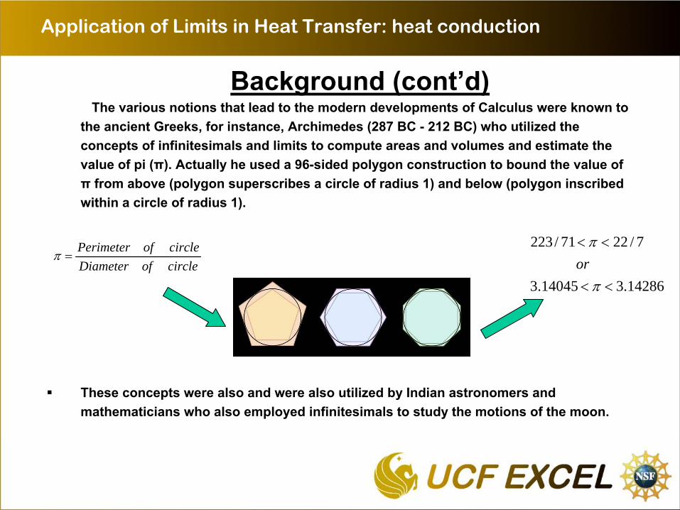
Background (cont’d)The various notions that lead to the modern developments of Calculus were known to

the ancient Greeks, for instance, Archimedes (287 BC -

212 BC) who utilized theconcepts of infinitesimals and limits to compute areas and volumes and estimate the value of pi (π). Actually he used a 96-sided polygon construction to bound the value of π

from above (polygon superscribes

a circle of radius 1) and below (polygon inscribedwithin a circle of radius 1).

These concepts were also and were also utilized by Indian astronomers and mathematicians who also employed infinitesimals to study the motions of the moon.

14286.314045.3

7/2271/223

<<

<<

π

πorcircleofDiameter

circleofPerimeter=π


Background (cont’d)While several French, German, English and Dutch mathematicians contributed seminal concepts of what was to become modern Calculus, it was Isaac Newton (1643 - 1727 AD) and Gottfried Leibniz (1646 - 1716 AD), who are credited to have independently arrived at the Fundamental Theorem of Calculus, and defined and codified Calculus, its rules and its notations.

Gottfried Wilhelm Leibniz (1646-1716). A German philosopher (school of optimism), mathematician, physicist, and logician.

Discovered Calculus independently from Newton. Defined most of notation utilized today. Discovered the binary system.

Sir Issac

Newton (16443-1727). English mathematician, physicist, astronomer, and natural philosopher. Discovered Calculus independently from Leibniz. His monumental publication in 1687 of PhilosophiaeNaturalis Principia Mathematica, is considered by all scientists, mathematicians, and engineers to be one of the greatest and defining accomplishmentsin human history (described universal gravitation and

three laws of motion: foundation of classical mechanics).



Calculus is principally concerned with:

1. Differentiation: the instantaneous rate of change (slope) of the curve describing a function.

2. Integration: the area under that curve.

Newton and Leibniz determined is that the two processes are related, and that integration is the inverse of differentiation.

Established certain notations as well rigorous rules and procedures to carry out both operationswhich taken all together constitute Calculus.

x

y

Area

y=f(x)slope



Relying heavily on Calculus, Newton laid out the basic principles describing gravitational attraction and the three laws of motion that are the groundwork of classical mechanics and the basis of modern engineering. Ever since, we have become very adept at utilizing derivatives and integrals to build mathematical models describing the physical processes around us.These models allow us to predict a wide variety of physical behaviors. The applications of Calculus prevade our lives, and they range for example, from understanding how a toy top spins and gyroscopes work, to how to make spaceships reach the moon and return, how to predict the future behavior of the weather, how to model and control how fluids and heat flow, how do design machines, and how to model and harness electricity and magnetism.

EXAMPLE:

Function

Dependent variable

Independent variable

Instantaneous Rate of change (derivative)x(t)

position of particle, x

time, t

velocity, v(t) v(t) velocity of particle, v time, t acceleration, a(t)T(x) temperature, T spatial location, x related to heat flow rate from hot wall

wall to cold



notion of the limit is central to understanding the two basic operations in calculus: the derivative and the integral.

What we mean by taking a limit of a function:

is to evaluate the behavior of that function, f, as the variable on which it depends, x, tends towards a particular value, xo .

Often the value of the variable is a finite constant, however, in many cases we are interested in what happens when the constant is zero or value of the constant tends to negative or positive infinity.

We will consider the notion of the limit in the context of its applications to mathematicaldefinitions and to physical problems.

)(lim xfoxx→

)(lim0

xfx→

lim ( )x

f x→−∞

lim ( )x

f x→+∞


2. Limits:

Evaluate the function: as x->1, that is take

As x -> 1 denominator goes to zero. Let’s compute f(x) as we approach from the left and right of 1 and:

So that the function seems to approach the value of 0.5, and indeed


Limits (cont’d)

if we were to ask what is the limit of as x ->-1 , then we would find that

Which is undefined as is evident when we examine the limit from the left and right of -1

Since the limit of f(x) from the left does not equal the limit from the right at x= -1, the limit is undefined and has to be interpreted depending on how x= -1 is approached.


Limits (cont’d)

We can use the symbolic manipulator capabilities of MATHCAD (actually the MAPLE engine) to take the limit as well:


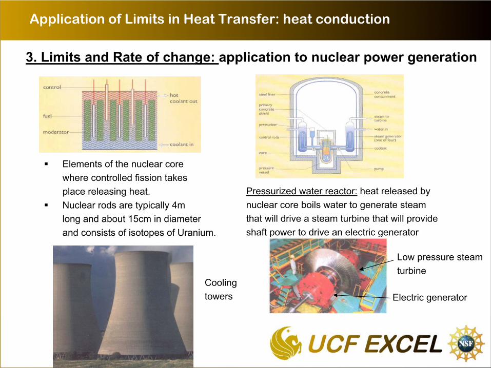
3. Limits and Rate of change: application to nuclear power generation

Pressurized water reactor:

heat released by nuclear core boils water to generate steamthat will drive a steam turbine that will provide shaft power to drive an electric generator

Elements of the nuclear core where controlled fission takes place releasing heat.Nuclear rods are typically 4mlong and about 15cm in diameterand consists of isotopes of Uranium.

Electric generator

Low pressure steam turbine

Cooling towers


Limits and Rate of change (cont’d)

Carnot efficiency of heat engines high

lowhighT

TT −=η

Typical nuclear power plant arrangement

Note:

temperatures in Kelvin = oC

+ 273.15

Boiler = Nuclear reactor

Nicolas Léonard

Sadi

Carnot(1976-1832) French physicist and Military engineer. Published ReflectionsOn the Motive Power of FireIn 1824 and laid out foundationsof Thermodynamics: Carnot cycle,Carnot efficiency, second law of Thermodynamics…Considered the fatherOf Thermodynamics.

coolingtower


Limits and rate of change (cont’d)

Model as a slender bar that is 2L wide.Temperature distribution is given by:

Plot of T(x) for Tw=100oC and c= 101.9oC

0.05 0 0.05100

150

200

250

T x( )

x

x

05·10 -3

0.010.015

0.020.025

0.030.035

0.040.045

0.050.055

0.060.065

0.070.075

= T x( )

201.902201.449200.091197.826194.656190.58

185.598179.71

172.917165.217156.612147.101136.685125.362113.134

100

=Plot of T(x) for Tw=100oC and c= 101.9oC

0.05 0 0.05100

150

200

250

T x( )

x

x

05·10 -3

0.010.015

0.020.025

0.030.035

0.040.045

0.050.055

0.060.065

0.070.075

= T x( )

201.902201.449200.091197.826194.656190.58

185.598179.71

172.917165.217156.612147.101136.685125.362113.134

100

=



The average rate of change of temperature with respect x tofrom x1

= 0.065m to x2

= 0.075m is

The instantaneous rate of change of the temperature with respect to x is given by the limit*

* used rule number 3 of the limit laws in Section 2.3 of your Calculus book

X1

=0.065mX2

=0.075mT(0.065m)=125.362oCT(0.075m)=100oCΔx = x2

- x1

ΔT =T( x2

) -

T( x1

)

T(x2

)

Plot of T(x) for Tw=100oC and c= 101.9oC

0.05 0 0.05100

150

200

250

T x( )

x

T(x1

)

Δx

ΔT

instantaneous rate of change

of the temperature with respect to x

is linear



Average rate of change of temperature on [0.065m, 0.075m] can be computed as the mean of the instantaneous rates of change at these two locations, that is

where, we used the values

x

05·10 -3

0.010.015

0.020.025

0.030.035

0.040.045

0.050.055

0.060.065

0.070.075

= T x( )

201.902201.449200.091197.826194.656

190.58185.598

179.71172.917165.217156.612147.101136.685125.362113.134

100

= mT x( )

0-181.159-362.319-543.478-724.638-905.797

-1.087·10 3

-1.268·10 3

-1.449·10 3

-1.63·10 3

-1.812·10 3

-1.993·10 3

-2.174·10 3

-2.355·10 3

-2.536·10 3

-2.717·10 3

=

x=0x=-L x=L

Tw Tw

T(x)

x

Nuclearelementgenerates heat

x=0x=-L x=L

Tw Tw

T(x)

x


x=0x=-L x=L

Tw Tw

T(x)

x


The negative of the instantaneous rate of change of the temperature with position is related to the heat transferred from the rod into the water tomake it boil at Tw

= 100oC(relation for this is due to J.B. Fourier)



We can use the concept of limits to check is expressions make sense, that is we can as as the independent variable approachessome given value does the dependent variable approach someknown or appropriate value?

Consider our clicker question. The temperature between the hot and cold wall was given as

( ) ( )( )h c hxT x T T TL

= + −

Does this make sense? well we can check using the limiting behavior of the dependent variable, T, as the independent variable,x, approaches 0 and L since we know T(0)=Th

and T(L)=Tc

.



Check temperature solution in the limits of both ends of the wall:

1. check the limit as x->0:

2. check the limit as x->L: lim [ ( ) ]h c h cx L

xT T T TL→

⎛ ⎞+ − =⎜ ⎟

⎝ ⎠

0lim [ ( ) ]h c h hx

xT T T TL→

⎛ ⎞+ − =⎜ ⎟

⎝ ⎠

… and since the solution satisfies the imposed temperature on both ends of the wall the solution makes sense so far.



We can utilize this result to estimate the heat lost from the wall of the house.The thermal conductivity is a property that indicates the ability of materials to conduct (transfer) heat. It is measured and known for many materials

The heat transferred per unit area of the wall, q, is given by the relationship:

And using our temperatures and instantaneous rate of change of the temperature with respectto space, we obtain for our case of a 1ft thick wall of concrete:


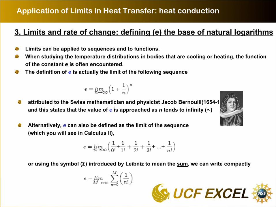
3. Limits and rate of change: defining (e) the base of natural logarithms

Limits can be applied to sequences and to functions. When studying the temperature distributions in bodies that are cooling or heating, the function of the constant e is often encountered.The definition of e is actually the limit of the following sequence

attributed to the Swiss mathematician and physicist Jacob Bernoulli(1654-1705), and this states that the value of e is approached as n tends to infinity (∞)

Alternatively, e can also be defined as the limit of the sequence (which you will see in Calculus II),

or using the symbol (Σ) introduced by Leibniz to mean the sum, we can write compactly

http://en.wikipedia.org/wiki/Image:Jakob_Bernoulli.jpg


Limits and rate of change: defining and ex

(cont’d)

A table and plot of this limit computed and plotted with the software package MATHCAD

show that to 15 digits:


Limits and rate of change: : defining and ex

(cont’d)

This number e is irrational, just like π

which can also be defined as a limit, and it occurs so oftenin analysis and physical systems that is called the "natural base" of logarithms.

The logarithm to be base e is denoted as ln(x)=loge (x).

We can also define the exponential function, f(x)=ex

which is plotted and tabulated below for various values of x

The exponential function appears often in practice in heat transfer (EML 4142), in electrical engineering (EGN 3373 and EEL 3304), in dynamics(EGN

3321), …


Limits and rate of change: defining and ex

(cont’d)

the behavior of the exponential function in terms of two limits when the independent variable x tends to a very large positive value (+∞

) and to a very large negative value (-∞), can be seen from the plot

Anywhere in between [- ∞,+ ∞] we can see that if we ask what is the value of for any we have a unique and finite value.

You will learn that you can represent the exponential function by an infinite polynomial, and that according to the rules of section 2.3, you can evaluate

that limit by substitution. For example,

As previously mentioned, we often use limits to check and guide us in our solutions, and the behavior of the exponential function as x-> -∞

and x-> +∞

will be important in the next applications lecture where we will study the behavior of the temperature in a cooling fin.


4. Limits and rate of change : temperature in a cooling fin

determine the temperature distribution in a cooling fin. Fins are designed to help improve the removal of heat and are ubiquitous in our world: car engine coolingsystem where fins are attached to the car radiator, computers where fins are attached to certain electronic chips to aid in removing waste heat.A fin of length, L, is being cooled by air at a temperature Tc

that is being forced over the fin by a fan.

cooling finsarranged in a computerto cool electronics


Limits and rate of change: temperature in a cooling fin (cont’d)

By applying the principles of conservation of energy and using methods you will learn in differential equations (MAP 2302), we can solve for the temperature to obtain

the general solution for the temperature, namely, that

where C1

and C2

are arbitrary constants and λ

depends on the fin geometry and material property as well as how fast the air is blowing over the fin.

From our experience with the exponential function, we know that for a very long fin (in the limit that x->∞),the temperature tends to infinity (which is non-physical) unless C2

= 0.

Thus, using the limiting behavior of the exponential function, we arrive at the conclusion that the general solution to the very long fin problem is

The remaining solution tells us that as the fin becomes very long, the temperature tends to that of the cooling air, Tc

, which makes physical sense.


Limits and rate of change: temperature in a cooling fin (cont’d)

The temperature distribution in a very long cooling fin is then

Plotted for a hot wall temperature of Tw =150 °C, a cooling air temperatureof Tc =25°, and taking a characteristic value of λ= 13.6 m-1, we see the solution satisfies the two limits,namely:

0 0.1 0.20

50

100

150

T x( )

Tc

x

Plot of the temperature x0

0.01

0.020.03

0.04

0.050.06

0.070.08

0.09

0.10.11

0.120.13

0.140.15

= T x( )150

134.037

120.113107.966

97.371

88.12980.067

73.03566.901

61.55

56.88252.811

49.25946.161

43.45941.102

=

Hot wallat temperatureTw

x

Cooling airat Tc

x=0 x=L

a

b

Copper cooling fin

fin cross-section

Q Heat flow

Hot wallat temperatureTw

x

Cooling airat Tc

x=0 x=L

a

b

Copper cooling fin

fin cross-section

Q Heat flow

We will use these results in our nextlecture


Conclusions

Calculus is concerned with differentiation and integration and the underlying concept is that of the limit.

we studied the concepts of limits and rates of change:1. limits –

what a function, sequence or seriestends to as a dependent variableapproaches a given value

2. rates of change –

slope of the function withrespect to the independent variable

Coming attractions: further applications of limits and rates of change to heat transfer

application of limits in heat transfer heat conduction · pdf fileapplication of limits in...

Documents