Chapter 2

1D heat conduction problems

2.1 1D heat conduction equation

When we consider one-dimensional heat conduction problems of a homogeneous isotropic solid, the Fourier equation simplifies to the form:

𝑐𝜌𝜕𝑇𝜕𝑡 =  𝜆

𝜕)𝑇𝜕𝑥) + 𝑄 (2.1)

If there is no heat generation, as is usually the case, such equation reduces to:

𝜕𝑇𝜕𝑡 = 𝑘

𝜕)𝑇𝜕𝑥) (2.2)

where 𝑘 =   ./0

. Furthermore, if the temperature distribution does not depend on time:

𝜕)𝑇𝜕𝑥) = 0 (2.3)

The stationary case of heat conduction in a one-dimension domain, like the one represented in figure 2.1, is particular simple to be solved.

Figure 2.1: the temperature within a solid media with prescribed Dirichelet boundary conditions

In fact, the general solution of the equation is in this case:

𝑇 𝑥 = 𝐴𝑥 + 𝐵 (2.4)

with A and B coefficients to be determined by imposing the boundary conditions.

Prescribed temperatures at both left and right surfaces:

𝑇456 =  𝑇7

𝑇458 =  𝑇9 (2.5)

we have:

𝑇7 = 𝐵 and 𝑇9 = 𝐴𝑙 +  𝑇7   or ;<=;>8

= 𝐴   (2.6)

In conclusion:

𝑇 𝑥 =  𝑇9 − 𝑇7

𝑙 𝑥 +  𝑇7 (2.7)

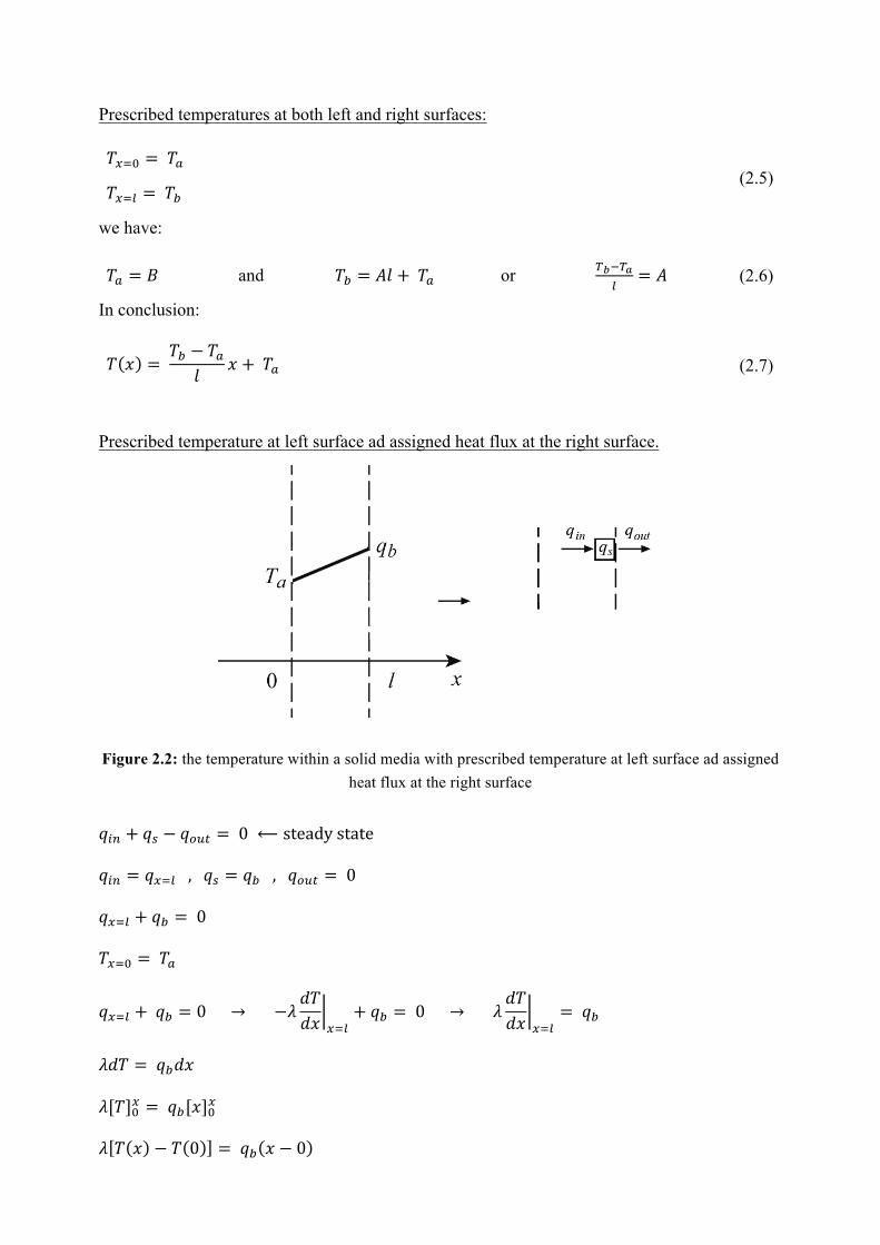
Prescribed temperature at left surface ad assigned heat flux at the right surface.

Figure 2.2: the temperature within a solid media with prescribed temperature at left surface ad assigned heat flux at the right surface

𝑞AB + 𝑞C − 𝑞DEF =  0   ⟵ steady  state  

𝑞AB = 𝑞458      ,      𝑞C = 𝑞9      ,      𝑞DEF =  0  

𝑞458 + 𝑞9 =  0  

𝑇456 =  𝑇7  

𝑞458 +  𝑞9 = 0           →            −𝜆𝑑𝑇𝑑𝑥 458

+ 𝑞9 =  0           →            𝜆𝑑𝑇𝑑𝑥 458

=  𝑞9      

𝜆𝑑𝑇 =  𝑞9𝑑𝑥  

𝜆[𝑇]64 =  𝑞9[𝑥]64  

𝜆 𝑇 𝑥 − 𝑇 0 =  𝑞9 𝑥 − 0  

𝜆 𝑇 𝑥 − 𝑇7 =  𝑞9𝑥  

𝑇 𝑥 =  𝑞9𝜆 𝑥 +  𝑇7  

 

Prescribed temperature at right side and assigned heat flux at left side

   

Figure 2.3: the temperature within a solid media with prescribed temperature at right side and assigned heat flux at left side

𝑞AB + 𝑞C − 𝑞DEF =  0   ⟵ steady  state  

𝑞AB = 0      ,      𝑞C = 𝑞7      ,      𝑞DEF =  𝑞456  

𝑞7 − 𝑞456 =  0  

𝑇458 =  𝑇9  

𝑞456  =   𝑞7        →            −𝜆𝑑𝑇𝑑𝑥 456

=  𝑞7          →            𝜆𝑑𝑇𝑑𝑥 456

=  −𝑞7  

𝜆𝑑𝑇 =  −𝑞7𝑑𝑥  

𝜆[𝑇]48 =  −𝑞7[𝑥]48  

𝜆 𝑇 𝑙 − 𝑇 𝑥 = −  𝑞7 𝑙 − 𝑥  

𝜆 𝑇9 − 𝑇 𝑥 = −  𝑞7 𝑙 − 𝑥  

𝑇 𝑥 =  𝑞7𝜆 𝑙 − 𝑥 +  𝑇9  

 

 

Convective and prescribed heat flux at both surfaces

 

Figure 2.4: the temperature distribution with convective and prescribed heat fluxes

Governing equation:

𝑑)𝑇𝑑𝑥) = 0 (2.8)

Boundary conditions:

𝑞S4FT + 𝑞7 − 𝑞456 = 0                   →                 ℎ7 𝑇V>  − 𝑇 +  𝑞7 + 𝜆𝑑𝑇𝑑𝑥 = 0                          𝑜𝑛      𝑥 = 0 (2.9)

𝑞458 +  𝑞9 −  𝑞S4FTT = 0                       →              −𝜆𝑑𝑇𝑑𝑥 +  𝑞9 −  ℎ9 𝑇 − 𝑇V<                          𝑜𝑛      𝑥 = 𝑙 (2.10)

where 𝑇V> and 𝑇V< are the temperatures of the surrounding media, 𝑞7 and 𝑞9 are surface heat generations per unit area per unit time, ℎ7 and ℎ9 are the heat transfer coefficients and subscripts a and b denote boundaries at 𝑥 = 0 and 𝑥 = 𝑙, respectively.

A general solution of eq. 2.8 is:

𝑇 𝑥 = 𝐴𝑥 + 𝐵 (2.11)

By substitution of the solution in eq. 2.9 and 2.10 we obtain:

𝜆𝐴 +  𝑞7 =  ℎ7 𝐴𝑥 + 𝐵 − 𝑇∞𝑎                  −𝜆𝐴 +  𝑞9 =  ℎ9 𝐴𝑥 + 𝐵 − 𝑇∞𝑏              

 

𝜆𝐴 + 𝑞7 =  ℎ7 𝐵 − 𝑇∞𝑎                          𝑝𝑒𝑟  𝑥 = 0  −𝜆𝐴 +  𝑞9 =  ℎ9 𝐴𝑙 + 𝐵 −  𝑇∞𝑏                  𝑝𝑒𝑟  𝑥 = 𝑙

 

The coefficients A and B are:

𝐴 =ℎ7ℎ9[ 𝑇∞𝑏 − 𝑇∞𝑎   +

𝑞9ℎ9−  𝑞7ℎ7

]

𝜆 ℎ7 + ℎ9 +  ℎ7ℎ9𝑙  

𝐵 =  𝑇∞𝑎  +𝑞7ℎ7+𝜆ℎ9 𝑇∞𝑏 − 𝑇∞𝑎   + (

𝑞9ℎ9−  𝑞7ℎ7

)

𝜆 ℎ7 + ℎ9 +  ℎ7ℎ9𝑙  

If no surface heat generation        𝑞7 =  𝑞9 = 0    

𝑇 𝑥 =  𝑇V>  + (𝑇V< −  𝑇V>  )ℎ9(ℎ7𝑥 +  𝜆)

𝜆 ℎ7 +  ℎ9 + ℎ7ℎ9𝑙   (2.12)

It is no possible to find a stationary solution by imposing an heat flux condition on both sides. In fact if 𝑞𝑎 and 𝑞𝑏 are not equal, the temperature response is not stationary since in presence of a variation of heat content, the temperature of the body should vary with time. If 𝑞𝑎 =  𝑞𝑏 the slope of the line is determined and the difference of temperature only can be obtained by no assumption on the temperature value. The case is analog to the mechanical response of an elastic spring free in the space at the end of which two forces with opposite sign are applied → rigid body motion

 

2.2 1D heat conduction: transient

Let us now consider a transient problem in which the temperature at x=0 is equal to Ta , the temperature at x=l is equal to zero and the initial condition is set as T=Ti(x). The governing equations read as follows

𝜕𝑇𝜕𝑡 =  

𝜆𝑐𝜌𝜕)𝑇𝜕𝑥) ,                  𝑘 =

𝜆𝑐𝜌 (2.13)

𝑇456 = 𝑇7 𝑇458 = 0 𝑇F56 =  𝑇A 𝑥 The solution is found by separation of variables, as we assume that the temperature can be expressed by the product of a function of position only f(x) and a function of time g(t)

( ) ( ) ( ), ,T x t f x g t= (2.14)

by substituting in the governing equation we obtain

2

2

( ) ( )( ) ( ) ,dg t d f xf x kg tdt dx

= (2.15)

that can also be written as

2

2

1 ( ) 1 ( ) ,( ) ( )dg t d f x

kg t dt f x dx= (2.16)

since the first member does not depend upon x, the second one does not depend upon t and the two members are equal, they can be set equal to a constant.

By setting the constant equal to -s2 we obtain two separate equations

2( ) ( ) 0,dg t ks g tdt

+ = (2.17)

And

22

2

( ) ( ) 0.d f x s f xdx

+ = (2.18)

The general solution of the first equation can be easily obtained by searching solution of the kind 𝑔 𝑡 = 𝑒bF and by finding the characteristic equation

2 0,ksα + = (2.19)

that leads to the general solution

𝑔 𝑡 = 𝑐c for 𝑠) = 0, 𝑔 𝑡 = 𝑐)𝑒=eCfF for 𝑠) ≠ 0 (2.20)

The general solution of the second equation can be sought in the same way or set directly as

𝑓 𝑥 = 𝑐i𝑥 +  𝑐j   for 𝑠) = 0

𝑓 𝑥 = 𝑐k sin 𝑠𝑥 +  𝑐n cos 𝑠𝑥   for 𝑠) ≠ 0 (2.21)

In conclusion the general solution of the original equation, that should be valid for arbitrary values of s can be written as

𝑇 𝑥, 𝑡 = 𝑒=eCfF 𝐴  sin 𝑠𝑥 +  𝐵 cos 𝑠𝑥   + 𝐶𝑥 + 𝐷 (2.22) with

2 5 2 6 1 3 1 4, , , .A c c B c c C c c D c c= = = = (2.23)

We now impose the satisfaction of boundary conditions by substituting then in the latter expression:

𝑇 0, 𝑡 = 𝐵𝑒=eCfF + 𝐷 =  𝑇7,

𝑇 𝑙, 𝑡 = 𝑒=eCfF 𝐴  𝑠𝑖𝑛  𝑠𝑙   + 𝐵 cos 𝑠𝑙 + 𝐶𝑙 + 𝐷 = 0 (2.24)

In order to satisfy the first equation for every value of t since 𝑒=eCfF   is never equal to zero it is necessary that

0, .aB D T= = (2.25)

For the second equation we have now 2

sin 0ks taAe sl Cl T− + + = (2.26)

that can only be satisfied for

sin 𝑠𝑙 = 0 and 𝐶 = −;>8

(2.27)

The values of k for which sin 𝑠𝑙 = 0 are

1,2,3...nns nlπ= = (2.28)

they are the eigenvalues of our problem.

The temperature can then be expanded in an infinite series of form

2

1( , ) 1 sin ,nks t

a n nn

xT x t T A e s xl

∞−

=

⎛ ⎞= − +⎜ ⎟⎝ ⎠∑ (2.29)

when An are unknown coefficients still to be determined. We now impose the initial condition 𝑇 𝑥, 0 = 𝑇A(𝑥) by substitution in the preceding equation we obtain

𝑇A 𝑥 − 𝑇7 1 −𝑥𝑙 =   𝐴B sin 𝑠B𝑥

V

B5c

(2.30)

In order to determine the coefficients An corresponding to initial condition we can profit of the properties of the sinusoidal function. In fact by multiplying both sides of the equation by sin 𝑠u𝑥  and integrating it from 0 to l (that is by finding the value of the scalar product between the terms at the first and the second member of the equation and the generic sinusoidal function sin 𝑠u𝑥  ) we obtain:

𝑠𝑖𝑛 𝑠B𝑥 sin 𝑠u𝑥𝑑𝑥 =  0              for        𝑚 ≠ 𝑛  8

6

𝑠𝑖𝑛) 𝑠B𝑥 𝑑𝑥 =  𝑙2              for        𝑚 = 𝑛  

8

6

(2.31)

And, for the coefficients An

0

2 ( ) 1 sin .l

n i a nxA T x T s xdx

l l⎡ ⎤⎛ ⎞= − −⎜ ⎟⎢ ⎥⎝ ⎠⎣ ⎦∫ (2.32)

In conclusion the expression of the temperature can be written as

2

01

2( , ) 1 { ( ) 1 sin }sin .nl ks t

a i a n nn

x xT x t T T x T s xdx s xel l l

∞−

=

⎡ ⎤⎛ ⎞ ⎛ ⎞= − + − −⎜ ⎟ ⎜ ⎟⎢ ⎥⎝ ⎠ ⎝ ⎠⎣ ⎦∑ ∫ (2.33)

From the form of the solution it is clear that the first term represents the stationary response that will eventually reached after a transient. The second term is on the contrary a time-dependent one, with the tendency of decaying to zero as time increases. In the case that different boundary conditions are imposed, say on both sides x=0,l imposed heat flux by convection, as expressed below

Figure 2.5: The temperature profile within a solid media which separates two semi-infinite fluid media. 𝑇V> and 𝑇V< correspond, respectively, to the temperature of the external media for x<0 and for x>l.

𝑞S4FT =  ℎ7 𝑇V>  − 𝑇

𝑞S4FTT =   ℎ9 𝑇 − 𝑇V<   (2.34)

with

𝑞S4FT + 𝑞7 − 𝑞 = 0  , 𝑞7 = 0           →           ℎ7 𝑇V>  − 𝑇 + 𝜆𝑑𝑇𝑑𝑥 = 0                          on      𝑥 = 0 (2.35)

𝑞 +  𝑞9 −  𝑞S4FTT = 0  , 𝑞9 = 0       →        −𝜆𝑑𝑇𝑑𝑥 −  ℎ9 𝑇 − 𝑇V<   = 0                    on      𝑥 = 𝑙 (2.36)

It is possible to use the same expression of the solution obtained before:

𝑇 𝑥, 𝑡 = 𝑒=eCfF 𝐴  𝑠𝑖𝑛  𝑠𝑥   + 𝐵 cos 𝑠𝑥   + 𝐶𝑥 + 𝐷 (2.37)

For obtaining the solution in this case similar steps can be followed to the ones used for the previous set of boundary conditions. The solution in this case will result as follows

𝑇 𝑥, 𝑡 = 𝑇V> + 𝑇V< − 𝑇V>

ℎ9 ℎ7𝑥 + 𝜆𝜆 ℎ7 + ℎ9 + ℎ7ℎ9𝑙

+

+2𝜆)𝑠B) + ℎ9) ℎ7 sin 𝑠B𝑥 + 𝜆𝑠B cos 𝑠B𝑥

𝑙 𝜆)𝑠B) + ℎ7) 𝜆)𝑠B) + ℎ9) + 𝑘 ℎ7 + ℎ9 𝜆)𝑠B) + ℎ7ℎ9

V

B5c

𝑒=eCfF..

𝑇A 𝑥 − 𝑇V> + 𝑇V< − 𝑇V>

ℎ9 ℎ7𝑥 + 𝜆𝜆 ℎ7 + ℎ9 + ℎ7ℎ9𝑙

ℎ7 sin 𝑠B𝑥8

6

+ 𝜆𝑠B cos 𝑠B𝑥 𝑑𝑥,

(2.38)

with sn being any positive root of the transcendental equation

( )2 2tan .a b

a b

s h hsl

s h hλλ

+=

− (2.39)

The stationary part of solution

𝑇 𝑥, 𝑡 → ∞ = 𝑇V> + 𝑇V< − 𝑇V>

ℎ9 ℎ7𝑥 + 𝜆𝜆 ℎ7 + ℎ9 + ℎ7ℎ9𝑙

(2.40)

can be further examined. In fact, the boundary condition in x=0 reads

𝑞7 = 𝜆𝑑𝑇𝑑𝑥 =  ℎ7 𝑇 − 𝑇V>   (2.41)

if the conductivity of the material is low or the convention thermal coefficient is high, the temperature on the wall reaches the temperature of the fluid 𝑇V> . In fact, with low λ and high ha

we have .{>≪ 1 and

𝜆ℎ7𝜕𝑇𝜕𝑥 = (𝑇 − 𝑇V>) (2.42)

with the first term of the equation equal to zero and 𝑇 = 𝑇V>. This results can also obtained from the above expression of the stationary part of the solution in presence of convective conditions on both sides, that can be written as

𝑇 𝑥 = 𝑇V> + 𝑇V< − 𝑇V>

ℎ9 ℎ7𝑥 + 𝜆𝜆 ℎ7 + ℎ9 + ℎ7ℎ9𝑙

= 𝑇V> + 𝑇V< − 𝑇V>

ℎ7ℎ9 𝑥 + 𝜆ℎ7

𝜆 ℎ7 + ℎ9 + ℎ7ℎ9𝑙

= 𝑇V> + 𝑇V< − 𝑇V>

𝑥 + 𝜆ℎ7

𝜆 1ℎ9+ 1ℎ7

+ 𝑙

(2.43)

and, considering the same assumption .{>≪ 1 and .

{<≪ 1 we finally have

𝑇 𝑥 = 𝑇V> + 𝑇V< − 𝑇V>48 . (2.44)

That is the temperature of the media at both sides of the solid can be directly assumed as the wall temperature. It is also interesting to note that, also with entering fluxes at both sides qa and qb, the temperature of the body T in the stationary response cannot have temperatures higher than the highest of the media by which the body is surrounded in perfect agreement with the physics of heat transfer. It is also obvious that, also in the presence of an entering flux, the body cannot increase indefinitely its temperature that cannot increase higher than the one from which the flux is generated.

Figure 2.6: The temperature within a wall with prescribed Dirichlet and Neumann boundary conditions

The 1D thermal behaviour just described can be applied to the case of an indefinite plate of thickness l with the side at isothermal condition where either the temperature, also variable with

the time t, or the heat flux can be applied. The same results are also valid for a one-dimensional solid (like a bar or a cable) with uniform section, provided that the lateral surface of the bar is isolated, that is no heat flux is present through it.

2.3 Honeycomb panel

Figure 2.7: Structure of a honeycomb sandwich panel: assembled view (A), and exploded view (with the two face sheets B, and the honeycomb core C). Ribbons run along the x direction, and are glued side

by side in counter-phase along the y direction as detailed.

Honeycomb panels (Figure 2.7) are structural elements with great stiffness-to-mass ratio, widely used in aerospace vehicles. Heat transfer through honeycomb panels is non-isotropic and difficult to predict. If the effect of the cover faces is taken aside, and convection and radiation within the honeycomb cells can be neglected in comparison with conduction along the ribbons (what is the actual case in aluminium honeycombs), heat transfer across each of the dimensions is:

𝑄4 = 𝜆𝐹4𝐴4∆𝑇4𝑙4

         with        𝐹4 =32𝛿𝑠

𝑄� = 𝜆𝐹�𝐴�∆𝑇�𝑙�

         with        𝐹� =𝛿𝑠

𝑄� = 𝜆𝐹�𝐴�∆𝑇�𝑙�          with        𝐹� =

83𝛿𝑠

(2.45)

where F is the factor modifying solid body conduction (the effective conductive area divided by the plate cross-section area), which is proportional to ribbon thickness, δ, divided by cell size, s (distance between opposite sides in the hexagonal cell, not hexagon side, a, in Figure 2.7; 𝑠 =3𝑎), and depends on the direction considered: x is along the ribbons (which are glued side by

side), y is perpendicular to the sides, and z is perpendicular to the panel. For instance, for the rectangular unit cell pointed out in Figure 2.7, of cross-section area 3as, the solid area is 8aδ, and the quotient is Fz=(8/3)δ/s.

Example

Evaluate the mean core-panel values of density and thermal conductivity through-the-thickness for a core made of aluminium foil with ρ=2700 kg/m3, λ=150 W/(m·K), thickness δ=30 μm and s=3 mm cell pattern.

Solution.

Fz = (8/3)(δ/s) = (8/3)(0.03/3) = 0.027

ρhoneycomb  = ρ· Fz = 2700·0.027=73 kg/ m3

λz honeycomb = λ· Fz = 150·0.027 = 4 W/(m·K).

2.4 Standard test method for thermal properties measurement

There are several standards to measure the thermal properties of a specimen. Here two methods based on ASTM C518 and C117.

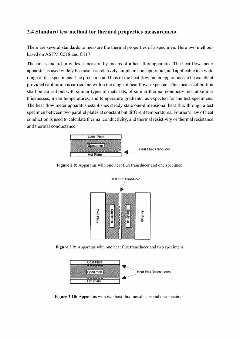
The first standard provides a measure by means of a heat flux apparatus. The heat flow meter apparatus is used widely because it is relatively simple in concept, rapid, and applicable to a wide range of test specimens. The precision and bias of the heat flow meter apparatus can be excellent provided calibration is carried out within the range of heat flows expected. This means calibration shall be carried out with similar types of materials, of similar thermal conductivities, at similar thicknesses, mean temperatures, and temperature gradients, as expected for the test specimens. The heat flow meter apparatus establishes steady state one-dimensional heat flux through a test specimen between two parallel plates at constant but different temperatures. Fourier’s law of heat conduction is used to calculate thermal conductivity, and thermal resistivity or thermal resistance and thermal conductance.

Figure 2.8: Apparatus with one heat flux transducer and one specimen.

Figure 2.9: Apparatus with one heat flux transducer and two specimens.

Figure 2.10: Apparatus with two heat flux transducers and one specimen.

The general features of a heat flow meter apparatus with the specimen or the specimens installed are shown in Figures 2.8, 2.9 and 2.10. A heat flow meter apparatus consists of two isothermal plate assemblies, one or more heat flux transducers and equipment to control the environmental conditions when needed. The two plate assemblies should provide isothermal surfaces in contact with either side of the test specimen. The assemblies consist of heat source or sink, a high conductivity surface, means to measure surface temperature, and means of support. A heat flux transducer may be attached to one, both, or neither plate assembly, depending upon the design. In all cases, the area defined by the sensor of the heat flux transducer is called the metering area and the remainder of the plate is the guard area. The two plate assemblies provide isothermal surfaces in contact with either side of the test specimen. The surfaces of the plate assemblies in contact with the specimen(s) shall be instrumented with precision temperature sensors such as thermocouples, platinum resistance thermometers (RTD), and thermistors.

When only one specimen is used, the thermal conductivity is calculated as follows:

𝜆 = 𝑆  𝑞  𝐿Δ𝑇 (2.46)

where 𝑆 is the calibration factor of the heat flux transducer (W/m2)/V.

The uncertainties in S, q, L, and Δ𝑇 (𝛿𝑆, 𝛿𝑞, 𝛿𝐿 and 𝛿Δ𝑇) can be used to form the uncertainty 𝛿𝜆 by the usual error propagation formula where the total uncertainty is calculated from the square root of the sums of the squares of the individual standard deviations.

𝛿𝜆𝜆

)

=𝛿𝑆𝑆

)

+𝛿𝑞𝑞

)

+𝛿𝐿𝐿

)

+𝛿Δ𝑇Δ𝑇

)

(2.47)

When two specimens (a and b) are used, the average thermal conductivity is calculated as follows:

𝜆7�S = 𝑆  𝑞2  

𝐿7 + 𝐿9Δ𝑇7 + Δ𝑇9

(2.48)

Another method to evaluate the thermal properties of a material is the standard ASTM C117. A general arrangement of the mechanical components of the apparatus is illustrated in Figure 2.11. This consists of a hot surface assembly comprised of a metered section and a primary guard, two cold surface assemblies, and secondary guarding in the form of edge insulation, a temperature-controlled secondary guard(s), and often an environmental chamber. Some of the components illustrated in Figure 2.11 are omitted in systems designed for ambient conditions, although a controlled laboratory environment is still required; edge insulation and the secondary guard are typically used only at temperatures that are more than ±10°𝐶 from ambient. At ambient conditions, the environmental chamber is recommended to help eliminate the effects of air movement within the laboratory and to help ensure that a dry environment is maintained.

Figure 2.11: General arrangement of the mechanical components of the guarded-hot-plate apparatus.

The purpose of the hot surface assembly is to produce a steady-state, one-dimensional heat flux through the specimens. The purpose of the edge insulation, secondary guard, and environmental chamber is to restrict heat losses from the outer edge of the primary guard. The cold surface assemblies are isothermal heat sinks for removing the energy generated by the heating units; the cold surface assemblies are adjusted so they are at the same temperature.

Figure 2.12: Illustration of idealized heat flow in a guarded-hot-plate apparatus.