application of qmc methods to pdes with random coefficients workshop/uqaw2016-talks... · frances...
TRANSCRIPT

Frances Kuo @ UNSW Australia p.1
Application of QMC methods toPDEs with random coefficients− a survey of analysis and implementation
Frances Kuo
University of New South Wales, Sydney, Australia
joint work withIvan Graham and Rob Scheichl (Bath), Dirk Nuyens (KU Leuven),
Christoph Schwab (ETH Zurich), Elizabeth Ullmann (Hamburg),Josef Dick, Thong Le Gia, James Nichols, and Ian Sloan (UNSW)
∼ Based on a survey of the same title, written jointly with Dirk Nuyens ∼

Frances Kuo @ UNSW Australia p.2
Outline
Motivating example – a flow through a porous medium
Quasi-Monte Carlo (QMC) methods
Component-by-component (CBC) construction
Application of QMC theory to PDEs with random coefficients
estimate the norm
choose the “weights”
Software
http://people.cs.kuleuven.be/~dirk.nuyens/qmc4pde
Concluding remarks

Frances Kuo @ UNSW Australia p.3
Motivating exampleUncertainty in groundwater flow
eg. risk analysis of radwaste disposal or CO2 sequestration
Darcy’s law q + a ~∇p = f
mass conservation law ∇ · q = 0in D ⊂ R
d, d = 1, 2, 3
together with boundary conditions
[Cliffe, et. al. (2000)]
Uncertainty in a(xxx, ω) leads to uncertainty in q(xxx, ω) and p(xxx, ω)

Frances Kuo @ UNSW Australia p.4
Expected values of quantities of interestTo compute the expected value of some quantity of interest:
1. Generate a number of realizations of the random field(Some approximation may be required)
2. For each realization, solve the PDE using e.g. FEM / FVM / mFEM
3. Take the average of all solutions from different realizations
This describes Monte Carlo simulation.
Example : particle dispersion
p = 1 p = 0
∂p∂~n
= 0
∂p∂~n
= 0
◦release point →•
0
0.2
0.4
0.6
0.8
1
0 0.2 0.4 0.6 0.8 1

Frances Kuo @ UNSW Australia p.4
Expected values of quantities of interestTo compute the expected value of some quantity of interest:
1. Generate a number of realizations of the random field(Some approximation may be required)
2. For each realization, solve the PDE using e.g. FEM / FVM / mFEM
3. Take the average of all solutions from different realizations
This describes Monte Carlo simulation.
NOTE: expected value = (high dimensional) integral
s = stochastic dimension
→ use quasi-Monte Carlo methods
103
104
105
106
10−5
10−4
10−3
10−2
10−1
error
n
n−1/2
n−1
or better QMC
MC

Frances Kuo @ UNSW Australia p.5
MC v.s. QMC in the unit cube∫
[0,1]sF (yyy) dyyy ≈ 1
n
n∑
i=1
F (ttti)
Monte Carlo method Quasi-Monte Carlo methodsttti random uniform ttti deterministic
n−1/2 convergence close to n−1 convergence or better
0 1
1
64 random points
••
•
••
•
•
•
•
•
•
•••
•
•
••
•
•
•
•
•
•
•
•
•
•
•
•
•
•
•
•
•
•
•
•
•
•
•
••
• •
•
••
•
•
•
••
••
•
•
•
•
•
•
••
•
0 1
1
First 64 points of a2D Sobol′ sequence
•
•
•
•
•
•
•
•
•
•
•
•
•
•
•
•
•
•
•
•
•
•
•
•
•
•
•
•
•
•
•
•
•
•
•
•
•
•
•
•
•
•
•
•
•
•
•
•
•
•
•
•
•
•
•
•
•
•
•
•
•
•
•
•
0 1
1
A lattice rule with 64 points
•
•
•
•
•
•
•
•
•
•
•
•
•
•
•
•
•
•
•
•
•
•
•
•
•
•
•
•
•
•
•
•
•
•
•
•
•
•
•
•
•
•
•
•
•
•
•
•
•
•
•
•
•
•
•
•
•
•
•
•
•
•
•
•
more effective for earlier variables and lower-order projectionsorder of variables irrelevant order of variables very important
use randomized QMC methods for error estimation

Frances Kuo @ UNSW Australia p.6
QMCTwo main families of QMC methods:
(t,m,s)-nets and (t,s)-sequenceslattice rules
0 1
1
First 64 points of a2D Sobol′ sequence
•
•
•
•
•
•
•
•
•
•
•
•
•
•
•
•
•
•
•
•
•
•
•
•
•
•
•
•
•
•
•
•
•
•
•
•
•
•
•
•
•
•
•
•
•
•
•
•
•
•
•
•
•
•
•
•
•
•
•
•
•
•
•
•
0 1
1
A lattice rule with 64 points
•
•
•
•
•
•
•
•
•
•
•
•
•
•
•
•
•
•
•
•
•
•
•
•
•
•
•
•
•
•
•
•
•
•
•
•
•
•
•
•
•
•
•
•
•
•
•
•
•
•
•
•
•
•
•
•
•
•
•
•
•
•
•
•
(0,6,2)-netHaving the right number ofpoints in various sub-cubes
A group under addition modulo Z
and includes the integer points
•
•
•
•
•
•
•
•
•
•
•
•
•
•
•
•
•
•
•
•
••
•
••
• •
•
•
••
•
•
•
•
•
•
•
• ••
•
•
•
•
•
•
•
•
•
•
•
•
•
Niederreiter book (1992)
Sloan and Joe book (1994)
Important developments:component-by-component (CBC ) construction , “fast” CBChigher order digital nets
Dick and Pillichshammer book (2010)
Dick, Kuo, Sloan Acta Numerica (2013)
Nuyens and Cools (2006)Dick (2008)

Frances Kuo @ UNSW Australia p.7
Application of QMC to PDEs with random coefficients
[0] Graham, K., Nuyens, Scheichl, Sloan (J. Comput. Physics, 2011)
[1] K., Schwab, Sloan (SIAM J. Numer. Anal., 2012)
[2] K., Schwab, Sloan (J. FoCM, 2015)
[3] Graham, K., Nichols, Scheichl, Schwab, Sloan (Numer. Math., 2015)
[4] K., Scheichl, Schwab, Sloan, Ullmann (in review)
[5] Dick, K., Le Gia, Nuyens, Schwab (SIAM J. Numer. Anal., 2014)
[6] Dick, K., Le Gia, Schwab (in review)
[7] Graham, K., Nuyens, Scheichl, Sloan (in progress)
AlsoSchwab (Proceedings of MCQMC 2012)
Le Gia (Proceedings of MCQMC 2012)
Dick, Le Gia, Schwab (in review)
Harbrecht, Peters, Siebenmorgen (Math. Comp., 2015)
Gantner, Schwab (Proceedings of MCQMC 2014)
Robbe, Nuyens, Vandewalle (Master thesis of Robbe, 2015)
Ganesh, Hawkings (SIAM J. Sci. Comput., 2015)

Frances Kuo @ UNSW Australia p.9
Application of QMC to PDEs with random coefficients
Three different QMC theoretical settings:
[1,2] Weighted Sobolev space over [0, 1]s and “randomly shifted lattice
rules”
[3,4] Weighted space setting in Rs and “randomly shifted lattice rules”
[5,6] Weighted space of smooth functions over [0, 1]s and (deterministic)
“interlaced polynomial lattice rules”
Uniform Lognormal LognormalKL expansion KL expansion Circulant embedding
Experiments only [0]*First order, single-level [1] [3]* [7]*First order, multi-level [2] [4]*Higher order, single-level [5]Higher order, multi-level [6]*
The * indicates there are accompanying numerical results
AIM OF THIS TALK: to survey [1,2] , [3,4] , [5,6] in a unified view

Frances Kuo @ UNSW Australia p.10
5-minute QMC primer
Common features among all three QMC theoretical settings:
Separation in error bound
(rms) QMC error ≤ (rms) worst case error γγγ × norm of integrand γγγ(rms) QMC error ≤ (rms) worst case error γγγ × norm of integrand γγγ
Weighted spaces
Pairing of QMC rule with function space
Optimal rate of convergence
Rate and constant independent of dimension
Fast component-by-component (CBC) construction
Extensible or embedded rules
Application of QMC theory
Estimate the norm (critical step)
Choose the weights
Weights as input to the CBC construction

Frances Kuo @ UNSW Australia p.11
Application of QMC to PDEs with random coefficients
Three different QMC theoretical settings:
[1,2] Weighted Sobolev space over [0, 1]s and “randomly shifted lattice
rules”
[3,4] Weighted space setting in Rs and “randomly shifted lattice rules”
[5,6] Weighted space of smooth functions over [0, 1]s and (deterministic)
“interlaced polynomial lattice rules”
Uniform Lognormal LognormalKL expansion KL expansion Circulant embedding
Experiments only [0]*First order, single-level [1] [3]* [7]*First order, multi-level [2] [4]*Higher order, single-level [5]Higher order, multi-level [6]*
The * indicates there are accompanying numerical results

Frances Kuo @ UNSW Australia p.12
Lattice rulesRank-1 lattice rules have points
ttti = frac
(i
nzzz
)
, i = 1, 2, . . . , n
zzz ∈ Zs – the generating vector, with all components coprime to n
frac(·) – means to take the fractional part of all components
0 1
1
A lattice rule with 64 points
•
•
•
•
•
•
•
•
•
•
•
•
•
•
•
•
•
•
•
•
•
•
•
•
•
•
•
•
•
•
•
•
•
•
•
•
•
•
•
•
•
•
•
•
•
•
•
•
•
•
•
•
•
•
•
•
•
•
•
•
•
•
•
•

Frances Kuo @ UNSW Australia p.12
Lattice rulesRank-1 lattice rules have points
ttti = frac
(i
nzzz
)
, i = 1, 2, . . . , n
zzz ∈ Zs – the generating vector, with all components coprime to n
frac(·) – means to take the fractional part of all components
0 1
1
A lattice rule with 64 points
64
1
2
3
4
5
6
7
8
9
10
11
12
13
14
15
16
17
18
19
20
21
22
23
24
25
26
27
28
29
30
31
32
33
34
35
36
37
38
39
40
41
42
43
44
45
46
47
48
49
50
51
52
53
54
55
56
57
58
59
60
61
62
63
∼ quality determined by the choice of zzz ∼
n = 64 zzz = (1, 19) ttti = frac
(
i
64(1, 19)
)

Frances Kuo @ UNSW Australia p.13
Randomly shifted lattice rulesShifted rank-1 lattice rules have points
ttti = frac
(i
nzzz +∆∆∆
)
, i = 1, 2, . . . , n
∆∆∆ ∈ [0, 1)s – the shift
shifted by
∆∆∆ = (0.1, 0.3)
0 1
1
A lattice rule with 64 points
•
•
•
•
•
•
•
•
•
•
•
•
•
•
•
•
•
•
•
•
•
•
•
•
•
•
•
•
•
•
•
•
•
•
•
•
•
•
•
•
•
•
•
•
•
•
•
•
•
•
•
•
•
•
•
•
•
•
•
•
•
•
•
•
0 1
1
A shifted lattice rule with 64 points
•
•
•
•
•
•
•
•
•
•
•
•
•
•
•
•
•
•
•
•
•
•
•
•
•
•
•
•
•
•
•
•
•
•
•
•
•
•
•
•
•
•
•
•
•
•
•
•
•
•
•
•
•
•
•
•
•
•
•
•
•
•
•
•
∼ use a number of random shifts for error estimation ∼

Frances Kuo @ UNSW Australia p.14
Component-by-component construction
Want to find zzz with (shift-averaged) “worst case error ” as small possible.∼ Exhaustive search is practically impossible - too many choices! ∼
CBC algorithm [Sloan, K., Joe (2002);. . . ]
1. Set z1 = 1.2. With z1 fixed, choose z2 to minimize the worst case error in 2D.3. With z1, z2 fixed, choose z3 to minimize the worst case error in 3D.4. etc.
Cost of algorithm is only O(n logn s) using FFTs. [Nuyens, Cools (2006)]
Optimal rate of convergence O(n−1+δ) in “weighted Sobolev space”,
with the implied constant independent of s under an appropriatecondition on the weights. [K. (2003); Dick (2004)]
∼ Averaging argument: there is always one choice as good as average! ∼
Extensible/embedded variants. [Cools, K., Nuyens (2006);Dick, Pillichshammer, Waterhouse (2007)]
http://people.cs.kuleuven.be/~dirk.nuyens/fast-cbc/http://people.cs.kuleuven.be/~dirk.nuyens/qmc-generators/

Frances Kuo @ UNSW Australia p.15
Fast CBC construction [Nuyens, Cools (2006)]
Images by Dirk Nuyens, KU Leuven
n = 53
1
53
Natural ordering of the indices Generator ordering of the indices
Matrix-vector multiplication with a circulant matrix can be done using FFT

Frances Kuo @ UNSW Australia p.16
Fast CBC construction [Nuyens, Cools (2006)]
Images by Dirk Nuyens, KU Leuven
n = 128 = 27
1 2 4 8
16
32
64
128 1 2 4 8
16
32
64
128
① Natural ordering of the indices
② Grouping on divisors ③ Generator ordering of the indices
④ Symmetric reduction after application
of B2 kernel function

Frances Kuo @ UNSW Australia p.17
Standard QMC theory todayWorst case error bound
∣∣∣∣∣
∫
[0,1]sF (yyy) dyyy − 1
n
n∑
i=1
F (ttti)
∣∣∣∣∣≤ ewor(ttt1, . . . , tttn) ‖F‖
Weighted Sobolev space [Sloan, Wozniakowski (1998)]
∣∣∣∣∣
∫
[0,1]sF (yyy) dyyy − 1
n
n∑
i=1
F (ttti)
∣∣∣∣∣≤ ewor
γγγ (ttt1, . . . , tttn) ‖F‖γγγ
‖F‖2γγγ =
∑
u⊆{1:s}
1
γu
∫
[0,1]|u|
∣∣∣∣∣
∂|u|F
∂yyyu
(yyyu; 0)
∣∣∣∣∣
2
dyyyu
2s subsets “anchor” at 0 (also “unanchored”)“weights” Mixed first derivatives are square integrable
Small weight γu means that F depends weakly on the variables yyyu
Choose weights to minimize the error bound [K., Schwab, Sloan (2012)](
2
n
∑
u⊆{1:s}
γλuau
)1/(2λ)
︸ ︷︷ ︸
bound on worst case error (CBC)
(∑
u⊆{1:s}
bu
γu
)1/2
︸ ︷︷ ︸
bound on norm
⇒ γu =
(bu
au
)1/(1+λ)
Construct points (CBC) to minimize the worst case error
“POD weights”

Frances Kuo @ UNSW Australia p.18
Application of QMC to PDEs with random coefficients
Three different QMC theoretical settings:
[1,2] Weighted Sobolev space over [0, 1]s and “randomly shifted lattice
rules”
[3,4] Weighted space setting in Rs and “randomly shifted lattice rules”
[5,6] Weighted space of smooth functions over [0, 1]s and (deterministic)
“interlaced polynomial lattice rules”
Uniform Lognormal LognormalKL expansion KL expansion Circulant embedding
Experiments only [0]*First order, single-level [1] [3]* [7]*First order, multi-level [2] [4]*Higher order, single-level [5]Higher order, multi-level [6]*
The * indicates there are accompanying numerical results

Frances Kuo @ UNSW Australia p.19
QMC theory for integration over Rs
Change of variables∫
Rs
F (yyy)s∏
j=1
φ(yj) dyyy =
∫
[0,1]sF (Φ−1(www)) dwww
Norm with weight function [Nichols & K. (2014)]
‖F‖2γγγ =
∑
u⊆{1:s}
1
γu
∫
R|u|
∣∣∣∣∣
∂|u|F
∂yyyu
(yyyu; 0)
∣∣∣∣∣
2∏
j∈u
ϕ2j (yj) dyyyu
weight function
Also unanchored variantRandomly shifted lattice rules CBC error bound for general weights γuConvergence rate depends on the relationship between φ and ϕj
Fast CBC for POD weights

Frances Kuo @ UNSW Australia p.20
Application of QMC to PDEs with random coefficients
Three different QMC theoretical settings:
[1,2] Weighted Sobolev space over [0, 1]s and “randomly shifted lattice
rules”
[3,4] Weighted space setting in Rs and “randomly shifted lattice rules”
[5,6] Weighted space of smooth functions over [0, 1]s and (deterministic)
“interlaced polynomial lattice rules”
Uniform Lognormal LognormalKL expansion KL expansion Circulant embedding
Experiments only [0]*First order, single-level [1] [3]* [7]*First order, multi-level [2] [4]*Higher order, single-level [5]Higher order, multi-level [6]*
The * indicates there are accompanying numerical results

Frances Kuo @ UNSW Australia p.21
Higher order digital nets [Dick (2008)]
Classical polynomial lattice rule [Niederreiter (1992)]
n = bm points with prime b
An irreducible polynomial with degree m
A generating vector of s polynomials with degree < m
Interlaced polynomial lattice rule [Goda, Dick (2012)]
Interlacing factor α
An irreducible polynomial with degree m
A generating vector of αs polynomials with degree < m
Digit interlacing function Dα : [0, 1)α → [0, 1)
(0.x11x12x13 · · · )b, (0.x21x22x23 · · · )b, . . . , (0.xα1xα2xα3 · · · )b
becomes (0.x11x21 · · ·xα1x12x22 · · ·xα2x13x23 · · ·xα3
· · · )b
Weighted spaces with norm involving higher order mixed derivatives
Variants of fast CBC construction available[Dick, K., Le Gia, Nuyens, Schwab (2014)] “SPOD weights”

Frances Kuo @ UNSW Australia p.22
Properties of higher order digital nets
16 points obtained from a 4D Sobol′ sequence with interlacing factor 2:
Each rectangle contains exactly 2 points.
•
•
•
•
•
•
•
•
•
•
•
•
•
•
•
•

Frances Kuo @ UNSW Australia p.22
Properties of higher order digital nets
16 points obtained from a 4D Sobol′ sequence with interlacing factor 2:
Each rectangle contains exactly 2 points.
•
•
•
•
•
•
•
•
•
•
•
•
•
•
•
•

Frances Kuo @ UNSW Australia p.22
Properties of higher order digital nets
16 points obtained from a 4D Sobol′ sequence with interlacing factor 2:
The shaded area contains exactly 2 points.
•
•
•
•
•
•
•
•
•
•
•
•
•
•
•
•

Frances Kuo @ UNSW Australia p.22
Properties of higher order digital nets
16 points obtained from a 4D Sobol′ sequence with interlacing factor 2:
The shaded area contains exactly 2 points.
•
•
•
•
•
•
•
•
•
•
•
•
•
•
•
•
Frances Kuo @ UNSW Australia p.22
Properties of higher order digital nets
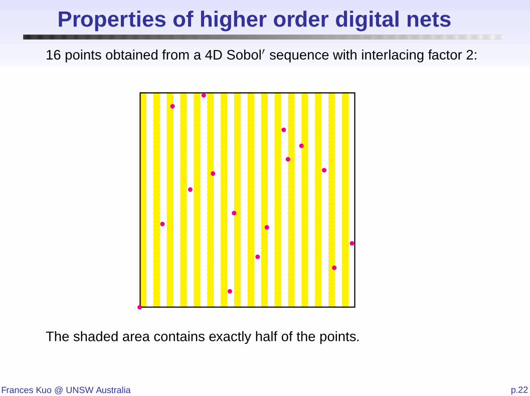
16 points obtained from a 4D Sobol′ sequence with interlacing factor 2:
The shaded area contains exactly half of the points.
•
•
•
•
•
•
•
•
•
•
•
•
•
•
•
•

Frances Kuo @ UNSW Australia p.23
Projections of higher order digital nets
Images by Dirk Nuyens, KU Leuven

Frances Kuo @ UNSW Australia p.24
Outline
Motivating example – a flow through a porous medium
Quasi-Monte Carlo (QMC) methods
Component-by-component (CBC) construction
Application of QMC theory to PDEs with random coefficients
estimate the norm
choose the “weights”
Software
http://people.cs.kuleuven.be/~dirk.nuyens/qmc4pde
Concluding remarks

Frances Kuo @ UNSW Australia p.25
Uniform v.s. lognormal
−∇ · (a(xxx,yyy)∇u(xxx,yyy)) = f(xxx), xxx ∈ D ⊂ Rd, d = 1, 2, 3
u(xxx,yyy) = 0, xxx ∈ ∂D
Uniform
a(xxx,yyy) = a0(xxx) +∑
j≥1
yj ψj(xxx), yj ∼ U [−12, 12]
Goal:∫
(−12,12)NG(u(·, yyy)) dyyy G – bounded linear functional
Key assumption: 0 < amin ≤ a(xxx,yyy) ≤ amax < ∞
Lognormal
a(xxx,yyy) = exp
(
a0(xxx) +∑
j≥1
yj ψj(xxx)
)
, yj ∼ N (0, 1)
Goal:∫
RN
G(u(·, yyy))∏
j≥1
φ(yj) dyyy =
∫
(0,1)NG(u(·,Φ-1(www))) dwww
Key assumption: restrict to yyy such that∑
j≥1|yj|‖ψj‖L∞ < ∞

Frances Kuo @ UNSW Australia p.26
Single-level v.s. multi-level (the uniform case)
I∞ =
∫
(−12,12)NG(u(·, yyy)) dyyy
Single-level algorithm
(1) dimension truncation
(2) FE discretization
(3) QMC quadrature
Deterministic:1
n
n∑
i=1
G(ush(·, ttti−1
21212))
Multi-level algorithm I∞ = (I∞ − IL) +∑L
ℓ=0(Iℓ − Iℓ−1), I−1 := 0
[Heinrich (1998); Giles (2008)]
Deterministic:L∑
ℓ=0
(1
nℓ
nℓ∑
i=1
G((usℓ
hℓ− u
sℓ−1
hℓ−1)(·, tttℓ,i−1
21212))
)

Frances Kuo @ UNSW Australia p.27
Estimate the norm (the uniform case)
Single-level algorithm
‖G(ush)‖γγγ
Multi-level algorithm
‖G(usℓ
hℓ− u
sℓ−1
hℓ−1)‖γγγ

Frances Kuo @ UNSW Australia p.27
Estimate the norm (the uniform case)
Single-level algorithm
‖G(ush)‖γγγ
∣∣∣∣
∂|u|
∂yyyu
G(ush(·, yyy))
∣∣∣∣=
∣∣∣∣G
(∂|u|
∂yyyu
ush(·, yyy)
)∣∣∣∣≤ ‖G‖H-1
∥∥∥∥
∂|u|
∂yyyu
ush(·, yyy)
∥∥∥∥H1
0
linearity and boundedness ofG
‖∂νννu(·, yyy)‖H1
0
= ‖∇∂νννu(·, yyy)‖L2≤ |ννν|!bbbννν ‖f‖H-1
amin
, bj :=‖ψj‖L∞
amin
‖G(ush)‖γγγ ≤ ‖f‖H-1‖G‖H-1
amin
(∑
u⊆{1:s}
(|u|!)2∏j∈ub2j
γu
)1/2

Frances Kuo @ UNSW Australia p.28
Choose the weights (the uniform case)
Single-level algorithm
‖G(ush)‖γγγ bj :=
‖ψj‖L∞
amin
ms-error .
(
2
n
∑
u⊆{1:s}
γuλ [ρ(λ)]|u|
)1/λ(∑
u⊆{1:s}
(|u|!)2∏j∈ub2j
γu
)
for all λ ∈ (12, 1]
Minimize the bound ⇒ POD weights γu =
(
|u|!∏
j∈u
bj√
ρ(λ)
)2/(1+λ)
If∑
j≥1 bpj < ∞, take λ =
1
2 − 2δfor δ ∈ (0, 1
2) when p ∈ (0, 2
3],
p
2 − pwhen p ∈ (2
3, 1).
The convergence rate is n−min(1−δ, 1p− 1
2).
The implied constant is independent of s.

Frances Kuo @ UNSW Australia p.29
Estimate the norm (the uniform case)
Single-level algorithm
‖G(ush)‖γγγ bj :=
‖ψj‖L∞
amin
Lemma 1
‖∇∂νννu(·, yyy)‖L2≤ |ννν|!bbbννν ‖f‖H-1
amin
Multi-level algorithm
‖G(usℓ
hℓ− u
sℓ−1
hℓ−1)‖γγγ
Lemma 2
‖∆∂νννu(·, yyy)‖L2. (|ννν| + 1)!bbb
ννν‖f‖L2
Lemma 3
‖∇∂ννν(u− uh)(·, yyy)‖L2. h(|ννν| + 2)!bbb
ννν‖f‖L2
Lemma 4
|∂νννG((u− uh)(·, yyy))|. h2(|ννν| + 5)!bbbννν‖f‖L2
‖G‖L2
bj :=max(‖ψj‖L∞ , ‖∇ψj‖L∞)
amin
‖∆∂νννu(·, yyy)‖L2. (|ννν| + 1)!bbb
ννν‖f‖L2
‖∇∂ννν(u− uh)(·, yyy)‖L2. h(|ννν| + 2)!bbb
ννν‖f‖L2
Important: FE projection depends on yyy
|∂νννG((u− uh)(·, yyy))| . h2(|ννν| + 5)!bbbννν‖f‖L2
‖G‖L2duality argument

Frances Kuo @ UNSW Australia p.30
Estimate the norm (the lognormal case)
Single-level algorithm
‖G(ush)‖γγγ
Lemma 5
‖∇∂νννu(·, yyy)‖L2≤ |ννν|!
(βββ
ln 2
)ννν ‖f‖H-1
amin(yyy)
Multi-level algorithm
‖G(usℓ
hℓ− u
sℓ−1
hℓ−1)‖γγγ
Lemma 6‖∆∂νννu(·, yyy)‖L2
. T (yyy)(|ννν| + 1)!(2βββ)ννν‖f‖L2
Lemma 7‖a1/2(·, yyy)∇∂ννν(u−uh)(·, yyy)‖L2
.hT (yyy)a1/2max(yyy)(|ννν|+2)!(2βββ)ννν‖f‖L2
Lemma 8|∂νννG((u− uh)(·, yyy))|. h2T 2(yyy)amax(yyy)(|ννν|+5)!(2βββ)ννν‖f‖L2
‖G‖L2
induction on ‖a1/2(·, yyy)∇∂νννu(·, yyy)‖L2
induction on ‖a−1/2(·, yyy)∇ · (a(·, yyy)∇∂νννu(·, yyy))‖L2
βj := ‖ψj‖L∞ =√µj ‖ξj‖L∞
‖∇∂νννu(·, yyy)‖L2≤ |ννν|!
(βββ
ln 2
)ννν ‖f‖H-1
amin(yyy)
βj := max(‖ψj‖L∞, ‖∇ψj‖L∞
)
‖∆∂νννu(·, yyy)‖L2. T (yyy)(|ννν| + 1)!(2βββ)ννν‖f‖L2
‖a1/2(·, yyy)∇∂ννν(u−uh)(·, yyy)‖L2.hT (yyy)a1/2
max(yyy)(|ννν|+2)!(2βββ)ννν‖f‖L2
|∂νννG((u− uh)(·, yyy))| . h2T 2(yyy)amax(yyy)(|ννν|+5)!(2βββ)ννν‖f‖L2‖G‖L2

Frances Kuo @ UNSW Australia p.31
Generic bound on mixed derivative
Mixed derivative bound For all multi-indices ννν ∈ {0, α}s we have
|∂νννF (yyy)| . ((|ννν| + a1)!)d1
s∏
j=1
(a2Bj)νj exp(a3Bj|yj|)
for integers α ≥ 1, a1 ≥ 0, real numbers a2 > 0, a3 ≥ 0, d1 ≥ 0, Bj > 0.
Particular cases:
F (yyy) =
G(ush) single-level
G(ushℓ
− ushℓ−1
) multi-level
Bj is bj, bj, βj, or βj
a3 = 0 =⇒ uniform case, a3 > 0 =⇒ lognormal case
Specify these parameters as input to the construction scripts:
http://people.cs.kuleuven.be/~dirk.nuyens/qmc4pde

Frances Kuo @ UNSW Australia p.32
MLQMC numerical results (the lognormal case)
D = (0, 1)2, f ≡ 1, homogeneous Dirichlet boundary
G(u(·, yyy)) = 1D∗
∫
D∗ u(xxx,yyy) dxxx, D∗ = (34, 78) × (7
8, 1)
Piecewise linear finite elements, off-the-shelf randomly shifted lattice rule
Matérn kernel: smoothness ν, variance σ2, correlation length scale λC
ǫ
10-4 10-3 10-2
Cos
t (in
sec
)
10-1
100
101
102
103
104
ν = 1.5, σ2 = 1, λ = 0.1
MCMLMCQMCMLQMC
2
3
ǫ
10-4 10-3 10-2
Cos
t (in
sec
)
10-1
100
101
102
103
104
ν = 2.5, σ2 = 0.25, λ = 1
MCMLMCQMCMLQMC
1
2
3
[K., Scheichl, Schwab, Sloan, Ullmann (in review)]

Frances Kuo @ UNSW Australia p.33
Application of QMC to PDEs with random coefficients
[0] Graham, K., Nuyens, Scheichl, Sloan (J. Comput. Physics, 2011)
[1] K., Schwab, Sloan (SIAM J. Numer. Anal., 2012)
[2] K., Schwab, Sloan (J. FoCM, 2015)
[3] Graham, K., Nichols, Scheichl, Schwab, Sloan (Numer. Math., 2015)
[4] K., Scheichl, Schwab, Sloan, Ullmann (in review)
[5] Dick, K., Le Gia, Nuyens, Schwab (SIAM J. Numer. Anal., 2014)
[6] Dick, K., Le Gia, Schwab (in review)
[7] Graham, K., Nuyens, Scheichl, Sloan (in progress)
Uniform Lognormal LognormalKL expansion KL expansion Circulant embedding
Experiments only [0]*First order, single-level [1] [3]* [7]*First order, multi-level [2] [4]*Higher order, single-level [5]Higher order, multi-level [6]*
The * indicates there are accompanying numerical results

Frances Kuo @ UNSW Australia p.34
Concluding remarks
QMC error bound can be independent of dimension
Three weighted space settings, fast CBC construction
Application of QMC theory: estimate the norm, choose the weights
Pairing of method and setting: best rate with minimal assumption
Theory versus practice
Affine parametric operator equations [Schwab (2013)]
Special orthogonality
Cost reduction: single-level versus multi-level n s h−d
Circulant embedding nh−d log(h−d)
Fast QMC matrix-vector multiplication n lognh−d
[Dick, K., Le Gia, Schwab (SIAM J. Sci. Comput., 2015)]
Multi-index methods [Haji-Ali, Nobile, Tempone (Numer. Math., 2015)]