Application of spectral derivative data in visible and near-infrared spectroscopy

This article has been downloaded from IOPscience. Please scroll down to see the full text article.

2010 Phys. Med. Biol. 55 3381

(http://iopscience.iop.org/0031-9155/55/12/008)

Download details:

IP Address: 147.188.192.41

The article was downloaded on 27/05/2010 at 16:21

Please note that terms and conditions apply.

View the table of contents for this issue, or go to the journal homepage for more

Home Search Collections Journals About Contact us My IOPscience

IOP PUBLISHING PHYSICS IN MEDICINE AND BIOLOGY

Phys. Med. Biol. 55 (2010) 3381–3399 doi:10.1088/0031-9155/55/12/008

Application of spectral derivative data in visible andnear-infrared spectroscopy

Hamid Dehghani1,2, Frederic Leblond2, Brian W Pogue2 andFabien Chauchard3

1 School of Computer Science, University of Birmingham, Birmingham B15 2TT, UK2 Thayer School of Engineering, Dartmouth College, NH 03755, USA3 Indatech, 385 Avenues des Baronnes, Prades Le Lez, France

E-mail: h.dehghani@cs.bham.ac.uk

Received 29 December 2009, in final form 6 April 2010Published 26 May 2010Online at stacks.iop.org/PMB/55/3381

AbstractThe use of the spectral derivative method in visible and near-infrared opticalspectroscopy is presented, whereby instead of using discrete measurementsaround several wavelengths, the difference between nearest neighbouringspectral measurements is utilized. The proposed technique is shown tobe insensitive to the unknown tissue and fibre contact coupling coefficientsproviding substantially increased accuracy as compared to more conventionaltechniques. The self-calibrating nature of the spectral derivative techniquesincreases its robustness for both clinical and industrial applications, as isdemonstrated based on simulated results as well as experimental data.

(Some figures in this article are in colour only in the electronic version)

1. Introduction

The use of near-infrared (NIR) spectroscopy in functional imaging of soft tissue relies on thelow absorption of tissue in the wavelength range of 650–900 nm, and is a widely used methodfor the measurement of tissue function and scattering properties (Bank et al 1998, Breit et al1997, Chance 2001, Colier et al 2001, Delpy and Cope 1997, Gopinath et al 1995, Manciniet al 1994, Matcher and Cooper 1994, Tromberg et al 2000, Leung et al 2009, Smith and Elwell2009). The advantages of NIR spectroscopy include the fact that light–matter interactionsin this spectral range are non-ionizing and that data acquisition can be performed on timescales compatible with several industry applications such as pharmaceutical powder (Torranceet al 2004) and polymer analysis (Lachenal 1998). Typically measurements of NIR lightepi-illumination and/or trans-illumination at two or more wavelengths are used to determinethe spectral absorption and scattering properties of tissue. Spectroscopy technique to date has

0031-9155/10/123381+19$30.00 © 2010 Institute of Physics and Engineering in Medicine Printed in the UK 3381

3382 H Dehghani et al

been used for the study of brain function (Smith and Elwell 2009), breast cancer detection andcharacterization (Shah et al 2001). Several other studies have combined the use of multiplesource and measurement NIR spectroscopy to topographically image brain activation studies(Fantini et al 1999, Taga et al 2003).

Due to recent instrumentation advancements, many current spectroscopy systems arecapable of measuring the complete spectrum of reflected and/or transmitted NIR signalsfollowing white light excitation with high bandwidth, therefore allowing the acquisition ofa comprehensive spectral dataset for the determination of tissue function and structure. Inseveral types of biological tissues the main chromophores contributing to absorption in the NIRare oxyhaemoglobin and deoxyhaemoglobin as well as, to a lesser extent, water. Moreoverthe intrinsic scattering properties of tissue have been shown to be closely related with bulktissue scatter size and density (Wang et al 2006). Additionally, through the use of novelspectral imaging techniques, it has been shown that by the direct incorporation of all spectralmeasurements simultaneously, it is possible to estimate tissue chromophore and scatteringproperties with improved quantitative and qualitative accuracy (Corlu et al 2005, Eames et al2008, Srinivasan et al 2005a).

Most spectroscopic measurements rely on pre-measurement calibration routines that areneeded to determine source strength and spectral characteristics as well as camera efficiencyand in the case of most systems, the calibration due to the optical fibre assembly andtissue contact. However, it is well accepted that fibre and tissue contact varies from caseto case and it may not be possible to allow for complete calibration to allow accuratespectral measurement and quantification. These parameters have a parasitic effect foronline application resulting in frequent and often difficult model maintenance (re-calibration).Recently, a novel NIR image reconstruction algorithm was developed that aims to recover thesefibre/tissue contact coefficients by their direct corporation within the imaging algorithms(Boas et al 2001). However, application of this technique may not be suitable in NIRspectroscopy since the addition of these unknowns can overwhelm the number of parametersrecovered.

The use of second differential NIR spectroscopy of water to determine the meanoptical path length of the neonatal brain has been previously demonstrated to monitor theabsolute cerebral concentration of deoxyhaemoglobin (Cooper et al 1996). Second-derivativepreprocessing of data has also been utilized to remove spectral baselines and dc offsets(Arakaki and Burns 1992). Second derivative analysis of visible data (500–650 nm) hasbeen shown to accentuate the differences between myoglobin and haemoglobin spectra and toremove baseline offsets between spectra, and decrease the effect of scattering on the spectra(Arakaki et al 2007). However, in the presence of noise in data, the use of second derivativemulti-spectral data can lead to over amplification of noise in the absolute evaluation of tissuefunction and physiology.

In a previous small animal NIR tomography study, the use of spectral derivative data hasbeen introduced (Xu et al 2005). It was demonstrated that instead of using NIR measurementsat each wavelength, when the difference between each neighbouring wavelength is insteadutilized, the resulting reconstructed images were insensitive to source and detector couplingand location. In this presented study, the theory and concept of spectral derivative method, asapplicable to NIR spectroscopy, is introduced. The underlying theory as to the self-calibratingnature of this technique is presented, together with the algorithm adapted for bulk parameterrecovery. Detailed simulated studies are presented whereby the effect of noise on the data isillustrated, together with preliminary experimental data demonstrating the effectiveness of theproposed method.

Application of spectral derivative data in visible and near-infrared spectroscopy 3383

Figure 1. Schematic of the reflectance spectroscopic measurements, where S denotes the source(placed at one scattering distance beneath the boundary) and D denotes the location of themeasurements at 50–100 mm away from the source with a 10 mm spacing.

2. Methods and results

2.1. Semi-infinite frequency domain analytical model

Consider a semi-infinite diffusive medium where scattering dominates over absorption with aphysical boundary at z = 0 associated with a finite index of refraction mismatch. For the zeroboundary condition, if the real source is at position rs = (xs, ys, zs), the image source will beat a position rs ′ = (xs ′ , ys ′ ,−zs ′). The excitation diffuse photon density wave is then given by(Li et al 1996)

�(r ′, rs) = vM0

D

[exp(ik|r ′ − rs |)

4π |r ′ − rs | − exp(ik|r ′ − rs ′ |)4π |r ′ − rs ′ |

], (1)

where �(r′,rs) is the fluence (J cm−2) at location r′ due to a source at rs, v is the speed of lightin the medium, D = v/3μ′

s , μ′s is the reduced scatter, k2 = (−vμa + iω)/D, μa is the absorption

coefficient, ω is the modulation frequency (ω = 2πf ), and M0 is the source dc intensity. Inorder to allow for a diffuse source to be modelled accurately, the location of the real sourceis modified so that it lies at one reduced scattering distance inside the z = 0 boundary, i.e. atzs = 1/μ′

s . Additionally, to allow for more accurate incorporation of the boundary condition,the zero-boundary condition is modified to the extrapolated boundary condition, so that thefluence vanishes on an extrapolated outer boundary (Haskell et al 1994). Therefore insteadof having a physical boundary at z = 0, an extrapolated boundary condition is imposed atze = 2AD where A is the boundary coefficient calculated using Fresnel’s law (Schweigeret al 1995). This would lead to a new image source rs′ at a position placed at zs = 2ze + 1/μ′

s .Although the frequency domain expression is defined in equation (1), the remainder of thepresented work will concentrate on continuous wave measurements for simplicity (intensityonly); however, all the presented work is valid for complex measurements.

2.2. Effect of unknown source and detector coupling coefficients

2.2.1. Spectral reflectance data analysis. Consider a set of reflectance spectroscopic pointmeasurements (Yi,j , for i = 1, . . . , n, where n is the total number of detectors, and j =1, . . . , L, where L is the total number of wavelengths) due to a point source (S) as shownin figure 1. The optical parameters within the volume of interest are given by absorption(μa) and reduced scattering coefficients (μ′

s), where μ′s = (1−g) μs where μs is the scattering

3384 H Dehghani et al

(a) (b)

Figure 2. The spectral response of tissue: (a) absorption due to oxyhaemoglobin (HbO),deoxyhaemoglobin (Hb) and water, and (b) reduced scatter based on Mie theory.

coefficient and g is the anisotropic factor. The tissue optical properties (absorption and reducedscatter) are a function of the wavelength of the applied source (λ), whose attenuation responsedepends on the concentration of each chromophore as well as on the scattering properties,as shown in figure 2 (Prahl 2009). Assuming the main absorbers to be oxyhaemoglobin(HbO), deoxyhaemoglobin (Hb) and water, Beer’s law can be used to compute overall tissueabsorption with reasonable accuracy:

μa(λ) =3∑

k=1

εk(λ)ck, (2)

where εk and ck are the molar absorption spectra and the concentration of the kth chromophore,respectively. The reduced scattering coefficient can be approximated using Mie theory(Mourant et al 1997):

μ′s = aλ−b, (3)

where a is assumed to be the scattering amplitude and b the scattering power. The coefficientμ′

s has units of inverse millimetres, and b is dimensionless so that scatter amplitude has unitsgiven by 10−3b(mm)b−1 and the wavelength is in micrometre (Srinivasan et al 2005b). Strictlyspeaking Mie theory is valid when interactions between scatter sites and photons can beconsidered to be elastic and when the scatter sites are spherical and independent scatter eventsare considered (Mourant et al 1998, Wang et al 2006). The reflectance measurements at eachdetector location Yi,j is then given by a light propagation model:

Yi,j = F(ck, a, b, λj , ri), (4)

where ri is the Euclidian distance of each detector from the source S. The model F used in thiswork is the semi-infinite analytical expression in equation (1), whereby for each wavelengthλ the absorption and scattering coefficients are calculated using equations (2) and (3). Thereflectance measurement Yi,j at each detector location and for each wavelength is proportionalto the source power and other coupling factors to the medium, which are absorbed into amultiplicative calibration factor NS. Similarly a calibration constant ND applies for the detectorgain factors, the coupling coefficients from the medium and the varying filter attenuation factors

Application of spectral derivative data in visible and near-infrared spectroscopy 3385

(a) (b)

Figure 3. Effect of the unknown source power and coupling coefficient (Ns) on the detector placed70 mm away from the source: (a) raw un-normalized data and (b) normalized data with respect tothe detector at 50 mm away from the source.

across the multi-spectral detection domain. Therefore, the detector measurement at each pointbecomes

Yi,j = NSNDF(c, a, b, λj , ri). (5)

Typically the source power and coupling coefficient NS are constant for all detectors (but mayalso vary spectrally for the un-calibrated system), whereas the detector gain and couplingcoefficient ND can vary by substantial amounts depending on the individual detector contactwith the medium as well as the detection optics setup (Boas et al 2001). In an experimentalsetup, although NS can be calculated to some accuracy and the data calibrated, these coefficientsdepend on each volume of interest and can vary substantially from case to case, as well as theintensity of the source may have a spectral dependence.

Consider a case whereby measurements are taken from an experimental setup asdepicted in figure 1. Reflectance boundary data Yi,j (intensity only at 100 MHz) have beencalculated for the wavelength range of 650–850 nm using the semi-infinite model based onequation (1) with typical chromophore concentrations of soft tissue consisting of HbO =0.01 mM, Hb = 0.01 mM, water = 75%, a = 0.87 and b = 1. A source is placed onescattering distance underneath the tissue surface, and detector measurements (henceforthreferred to as ‘noise-free’ data) have been calculated at six distances from 50 to 100 mm awayfrom the source. For the ‘noise-added’ data, a linear spectral dependence of the NS coefficients(90% – 75%, from 650 nm to 850 nm) is assumed with the detector coupling coefficients ND

taking values of 80%, 60%, 90%, 40%, 85% and 91% for detection points placed at 50, 60, 70,80, 90 and 100 mm, respectively. These simulated noise conditions are under the assumptionsthat for each specific wavelength, the source strength can vary by an unknown amount (butconstant for each source) and for each detector, due to the detector coupling coefficient, themeasured intensity can also vary by an unknown amount (but constant for each detector).

Figure 3(a) shows the log intensity plot from both the noise-free and noise-added data fora single detector point at 70 mm away from the source. The large variation seen between thedata represents the often unknown NS coefficient as well as ND. Nonetheless, it is often wellaccepted that in order to account for such variation in NS it is either possible to calibrate the datafor the unknown source strength using well-defined phantom experiments, or more commonlyin spectroscopic experiments to normalize each data point with respect to measurements at a

3386 H Dehghani et al

(a) (b)

(c)

Figure 4. Effect of detector gain factors and coupling coefficients (ND) at 780 nm: (a) rawun-normalized data and (b) normalized data with respect to the first detector point at 50 mm.(c) Percentage error between normalized noise-free and noise-added data.

given detector. In this latter approach, figure 3(b) shows the same data as in figure 3(a) butnormalized with respect to detector measurements at 50 mm away from the source. As evident,although such normalization could eliminate the effect of the unknown source strength, it doesnot however eliminate the effect of the unknown detector coupling coefficients ND becausethe two measurements used when ratioing are acquired at different tissue locations. Thecalculated error between the noise-free and noise-added data can be shown to equal the ratioof the modelled ND value at detectors 1 and 3, i.e. 12.5%.

Figure 4(a) shows the log intensity plot from both the noise-free and noise-added datafor all detectors at a single wavelength of 780 nm. The large variation between the twodatasets represents the unknown detector coupling coefficients ND. As in the previous case,it is possible to normalize the data with respect to measurements at a given detector. Inthis latter approach, figure 4(b) shows the same data as in figure 4(a) but normalized withrespect to detector measurements at 50 mm away from the source. As evident, although suchnormalization could eliminate the effect of the unknown source strength and ND at the detectorplaced at 50 mm, it does not however eliminate the effect of the unknown detector couplingcoefficients for all other detectors. It is worth noting that although the mismatched seenappears minimal, the calculated error, figure 4(c), corresponds to the ratio of the unknown ND

factors equalling an error of up to more than 40%.

Application of spectral derivative data in visible and near-infrared spectroscopy 3387

(a) (b)

(c)

Figure 5. Spectral derivative data for both noise-free and noise-added measurements at(a) 50 mm, and (b) 70 mm distance detectors. (c) Percentage error between normalized noise-freeand noise-added data for all detectors.

2.2.2. Spectral derivative reflectance data analysis. Assuming that the source and detectorcoupling coefficients have a small spectral dependence, that is NSj ∼ = NSj+1 and NDj ∼ =NDj+1, the spectral derivative method can be utilized to account for these unknown coefficients.Equation (5) can be modified such that

Yi,j+1

Yi,j

= NSj+1NDj+1F(c, a, b, λj+1, ri)

NSjNDjF (c, a, b, λj , ri)= F(c, a, b, λj+1, ri)

F (c, a, b, λj , ri). (6)

As evident by equation (6), assuming that the coupling coefficients between neighbouringwavelengths are equal, by taking the ratio of each dataset for each detector with respect to itsnearest wavelength, it is possible to eliminate the effect of these errors.

Using the same data as in the previous case, figure 5 shows the spectral derivative data(normalized log intensity plot of each wavelength with respect to its next highest wavelengthwith 2 nm separation) from both the noise-free and noise-added data for a single detectorpoint at 50 and 70 mm away from the source. As shown, despite a non-constant sourcecoupling coefficient, NSj, the spectral derivative calculations as derived in equation (6) allowself-calibration of data with respect to both the unknown coupling coefficients. Therefore theuse of spectral derivative data should in principle provide a much more accurate information

3388 H Dehghani et al

Figure 6. 2D FEM mesh used. The arrows indicate the location of the source and detectors.

regarding the spectrally dependent optical parameters. The percentage error for the spectralderivative data between the noise-free and noise-added dataset is shown in figure 5(c). It isseen that the maximum error seen is less than 0.2%, which is equal to the linear spectral errorvariation of NS.

2.3. Errors due to different models of light propagation

Many models and methods exist for the calculation of boundary data based on some inputsuch as geometry, optical properties and source/detector separation (Arridge 1999, Dehghaniet al 2009). Numerical models provide flexibilities in the number of degrees of freedomand they are computationally complex, whereas analytical models, although limited tosimple homogeneous cases, are computationally fast and efficient. Assuming that the truespectroscopic data from a domain is given by equation (1), it is possible to express any errordue to the model used as α, such that

Yi,j = αi,jF (c, a, b, λj , ri), (7)

where αi,j is the model error coefficient which can be detector dependent and a spectrallyvarying function. As in the previous example, if we assume that αi,j+1 ∼ = αi,j , then using thespectrally derived data, equation (5), it can be shown that the effect of such a scaling factorcan be ignored.

As an example, consider the same analytical data used in the previous section. Usingthe same optical parameters and source/detector geometry, equivalent spectral data werecalculated using a 2D and 3D finite element model (FEM) package, NIRFAST (Dehghaniet al 2008). A 2D model is used to assess the accuracy of such an approach, since thenumerical solutions of 2D models although not as accurate, are much faster than those of 3D.For the 2D model, figure 6, the domain consisted of a slab of length 200 mm and a thicknessof 100 mm, with the source placed at one scattering distance on the top face at 50 mm fromthe left boundary. The 2D FEM mesh consisted of 80 601 nodes corresponding to 160 000linear triangular elements. For the 3D FEM mesh, figure 7, the domain consisted of a slabwith a length (x-axis) of 140 mm, width (y-axis) of 100 mm and depth (z-axis) of 50 mm. Thesource was placed at one scattering distance on the top face at 20 mm from the left boundary.The 3D FEM mesh consisted of 49 098 nodes corresponding to 263 562 linear tetrahedralelements.

Application of spectral derivative data in visible and near-infrared spectroscopy 3389

(b)(a)

Figure 7. 3D FEM mesh used with the (a) x–z plane and (b) x–y plane. Note high density meshresolution in the source/detector locations.

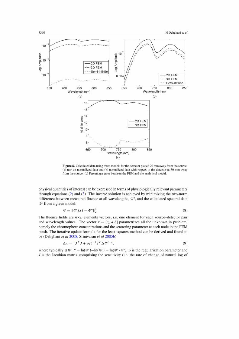
For both the 2D and 3D FEMs, as in the analytical case, detector measurements have beencalculated at a 50–100 mm distance away from the source on the same boundary. Figure 8(a)shows the log intensity plot from all the three models for a single detector point at 70 mmaway from the source. The large variation seen between the data represents the large mismatchseen between the three models. Figure 8(b) shows the same data in figure 8(a) but normalizedwith respect to detector measurements at 50 mm away from the source. As evident, althoughsuch normalization could eliminate the effect of the unknown model mismatch, it does nothowever eliminate the effect entirely. The calculated errors between the analytical models andthe FEMs are shown in figure 8(c). As seen, the largest error is found with the 2D model atabout 18%, whereas the 3D model has errors less than 9%.

Figure 9(a) shows the log intensity plot from all models at a single wavelength of 780 nm.Figure 9(b) shows the same data as in figure 9(a) but normalized with respect to detectormeasurements at 50 mm away from the source, and figure 9(c) shows the calculated errorbetween these data. Large errors can be seen between the FEMs and the analytical modelsranging up to 35% with the best results from the 3D model.

Figure 10 shows the spectral derivative data from all models for single detector points at50 and 70 mm away from the source. As shown, despite the use of three inherently differentmodels, the spectral derivative calculations allow self-calibration of data with respect to boththe unknown coupling coefficients and model mismatch parameter. The percentage error forthe derivative spectral data between FEMs and analytical models is shown in figure 10(c). It isseen that the maximum error seen for the 3D model is less than 0.3% and less than 0.85% forthe 2D model, which is much smaller than those shown in figures 8(c) and 9(c). Therefore theuse of spectral derivative data should in principle provide a much more accurate informationregarding the spectrally dependent optical parameters.

2.4. Inverse model

2.4.1. The spectral case. The goal of the inverse problem is the recovery of opticalparameters within the imaging domain based on the measurements of light fluence at the tissuesurface. This is accomplished based on a least-squares error optimization method allowing theformation of images in terms of the chromophore concentrations and the scattering parameters.This is done by assuming that light transport can be modelled as a diffusive process and that

3390 H Dehghani et al

(a) (b)

(c)

Figure 8. Calculated data using three models for the detector placed 70 mm away from the source:(a) raw un-normalized data and (b) normalized data with respect to the detector at 50 mm awayfrom the source. (c) Percentage error between the FEM and the analytical model.

physical quantities of interest can be expressed in terms of physiologically relevant parametersthrough equations (2) and (3). The inverse solution is achieved by minimizing the two-normdifference between measured fluence at all wavelengths, �o, and the calculated spectral data�c from a given model:

� = ‖�c(x) − �o‖22. (8)

The fluence fields are n×L elements vectors, i.e. one element for each source–detector pairand wavelength values. The vector x = [ck a b] parametrizes all the unknown in problem,namely the chromophore concentrations and the scattering parameter at each node in the FEMmesh. The iterative update formula for the least-squares method can be derived and found tobe (Dehghani et al 2008, Srinivasan et al 2005b)

x = (J T J + ρI)−1J T �c−o, (9)

where typically �c−o = ln(�c)−ln(�o) = ln(�c/�o), ρ is the regularization parameter andJ is the Jacobian matrix comprising the sensitivity (i.e. the rate of change of natural log of

Application of spectral derivative data in visible and near-infrared spectroscopy 3391

(a) (b)

(c)

Figure 9. Calculated data using three models for all detectors at 780 nm: (a) raw un-normalizeddata and (b) normalized data with respect to the first detector point at 50 mm. (c) Percentage errorbetween FEM and analytical models.

fluence with respect to a small change in x, δln�/δx) for each unknown parameter:

J = [Ja Jb Jc1 Jc2 Jc2 ] =

⎡⎢⎢⎢⎣

Ja,λ1 Jb,λ1 Jc1,λ1 Jc2,λ1 Jc3,λ1

Ja,λ2 Jb,λ2 Jc1,λ2 Jc2,λ2 Jc3,λ2

......

......

...

Ja,λjJb,λj

Jc1,λjJc2,λj

Jc3,λj

⎤⎥⎥⎥⎦ . (10)

2.4.2. The spectral derivative case. In the spectral derivative approach, the objective functionis modified from equation (8) to

�2 = ‖�′c−o‖22 =

∥∥∥∥∥∥∥∥∥∥

⎧⎪⎪⎪⎪⎨⎪⎪⎪⎪⎩

�cλ1

(x) − �cλ2

(x)

�cλ2

(x) − �cλ3

(x)

...

�cλj−1

(x) − �cλj

(x)

⎫⎪⎪⎪⎪⎬⎪⎪⎪⎪⎭

−

⎧⎪⎪⎪⎪⎨⎪⎪⎪⎪⎩

�oλ1

− �oλ2

�oλ2

− �oλ3

...

�oλj−1

− �oλj

⎫⎪⎪⎪⎪⎬⎪⎪⎪⎪⎭

∥∥∥∥∥∥∥∥∥∥

2

2

. (11)

Here �′c−o denotes the finite difference operator. Equation (9) can then be modified to

x = (J̃ T J̃ + ρI)−1J̃ T �′c−o, (12)

3392 H Dehghani et al

(a) (b)

(c)

Figure 10. Spectral derivative data for all light transport models at (a) 50 mm and (b) 70 mmdistance detectors. (c) Percentage error of derivative data between FEM and analytical models.

where

J̃ = [J̃ a J̃ b J̃ c1 J̃ c2 J̃ c2 ]

=

⎡⎢⎢⎢⎣

Ja,λ1 − Ja,λ2 Jb,λ1 − Jb,λ2 Jc1,λ1 − Jc1,λ2 Jc2,λ1 − Jc2,λ2 Jc3,λ1 − Jc3,λ2

Ja,λ2 − Ja,λ3 Jb,λ2 − Jb,λ3 Jc1,λ2 − Jc1,λ3 Jc2,λ2 − Jc2,λ3 Jc3,λ2 − Jc3,λ3

......

......

...

Ja,λj−1 − Ja,λjJb,λj−1 − Jb,λj

Jc1,λj−1 − Jc1,λjJc2,λj−1 − Jc2,λj

Jc3,λj−1 − Jc3,λj

⎤⎥⎥⎥⎦

(13)

and

�′c−o = ln

(�c

j−1

�oj−1

)− ln

(�c

j

�oj

)= ln

(�c

j−1 × �oj

�oj−1 × �c

j

). (14)

2.4.3. Simulated data. To demonstrate the flexibility of the proposed method, an approachbased on experimental design is used (Cela et al 2009) which has shown to be a robustand accurate method to decrease the total number of experiments or simulations in order tocalculate complete system responses for a large number of case scenarios (Nguyen et al 2008).In order to analyse the behaviour of the spectral derivative approach, several simulations were

Application of spectral derivative data in visible and near-infrared spectroscopy 3393

Table 1. The maximum and average (in parentheses) relative percentage error between the expectedand reconstructed parameter from noise-added simulated data. For each case ((a)–(c)) differenttypes of noise are added as described in section 2.4.3.

HbO Hb Water a b

Spectral derivative: case (a) 9.2 (2.4) 9.3 (2.4) 9.3 (3.2) 10.7 (2.8) 2.3 (0.8)Spectral derivative: case (b) 9.2 (2.4) 9.3 (2.4) 9.3 (3.2) 10.7 (2.8) 2.3 (0.8)Spectral derivative: case (c) 27.1 (15.8) 24.5 (13.4) 25.9 (13.4) 20.1 (11.4) 5.2 (2.8)

Spectral: case (a) 0.2 (0.06) 0.1 (0.04) 0.9 (0.1) 0.2 (0.05) 0.6 (0.1)Spectral: case (b) 250 (86) 279 (78) 602 (98) 1456 (359) 146 (45)Spectral: case (c) 1334 (121) 338 (84) 831 (111) 259 280 (5445) 874 (67)

run according to changes in HbO, Hb water, scattering amplitude (a) and scattering power(b) with the level of factors defined according to a central composite design. Five levels ofvariation were defined for each factor according to the central composite design, consistingof one central point, two axial points and two factorial points and the levels were calculatedin order to take into account the curvature of the surface response. A set of data are thereforecomposed of 52 experiments (run of simulation) for each approach and each type of addednoise with the maximum variations of chromophore concentrations and scattering parameters(as expected for soft tissue) given as HbO = 0.01–0.05 mM, Hb = 0.01–0.05 mM, water =30–90%, a = 0.2–1.2 and b = 0.5–1.5.

Reflectance spectral measurements from 650 to 850 nm (2 nm separation) were simulatedusing the model in equation (1) for a set of detectors ranging from 5 to 50 mm with 5 mmspacing (see figure 1). The simulated data were then corrupted using three types of noise: (a)1% randomly distributed Gaussian noise, (b) 1% randomly distributed Gaussian noise plusrandom (ranging from 0 to 100%) detector coupling coefficient (ND), and (c) 1% randomlydistributed Gaussian noise plus random detector coupling coefficient (ND) plus the linearvarying NS coefficient (80% – 75%, from 650 nm to 850 nm). These noise-added datasetswere then used together with equations (9) and (12) to reconstruct the chromophore andscattering parameters using the spectral and spectral-derivative techniques, respectively. Forthe inverse model, the regularization parameter ρ was set to 1% of the maximum of thediagonal of the matrix JTJ (or J̃

TJ̃ ) with a total of 50 iterations. The Jacobians were calculated

using the perturbation method (Arridge 1999) using equation (1) and the initial guess for allreconstructions was set as HbO = 0.03 mM, Hb = 0.03 mM, water = 50%, a = 1.0 andb = 1.0.

For each reconstructed model, the maximum and average relative error between eachof the expected and reconstructed parameter is shown in table 1. For case (a), the spectralmethod provides the smallest relative error as expected, since the only noise present in thedata is 1% random noise. Using the spectral derivative method, the results from case (a) andcase (b) are identical, demonstrating that the noise due to the detector coupling coefficient iseffectively cancelled, since spectral derivative data are used. However, the addition of thisdetector coupling coefficient demonstrated a large effect when conventional spectral methodis utilized, leading to errors well over 1000% for the recovery of scattering amplitude. Theresults from case (c) show that the spectral method has produced unreliable results, whereasthe spectral derivative method is still accurate within 27% in the worst scenario case, butgreatly improved as compared to the spectral method. This is not surprising as the effect ofthe source coupling coefficient is not entirely cancelled using the spectral derivative method.

3394 H Dehghani et al

2.4.4. Experimental data. A set of reflectance spectral measurements from 650 to 850 nm(2 nm separation) were acquired on the forearm of three human subjects, using the SAM-Spec R© system from Indatech. The measuring head is composed of a probe consisting of oneirradiating fibre bundle (2.5 mm diameter consisting of 55 fibres of 250 μm diameter) andthree measurement fibres (600 μm) which are fixed at pre-fabricated locations of 1.48, 2.78and 3.89 mm away from the source. The irradiation bundle was connected to a halogen lightsource (Leica CLS 150 XD). The spectral data at all detectors were measured using a Vis–NIRspectrometer (Zeiss, Vis–NIR enhanced, spectral range of 330–1100 nm). For each subject,three sets of spectral data were recorded at resting state, and were used together with the spectralderivative technique outlined above (equation (12)) and the semi-infinite model (equation (1))to calculate the bulk properties of total tissue haemoglobin (HbT), oxygen saturation (StO),water, scattering amplitude and scattering power. An example for the experimental spectralderivative data for a single subject, together with the fitted modelled data is shown infigure 11(a). The calculated average of each parameter, for each subject is shown infigure 11(b) together with the published bulk value of adipose tissue (Alexandrakis et al2005). It is seen that although the results from all subject show similar trends, the largestdiscrepancies are found between the values for water content (expected 50%, average for allsubjects of 17%) and scatter power (expected 5.3, average for all subjects of 25.5). There isa good agreement between the calculated oxygen saturation (expected 70%, average for allsubjects of 66.6%) as well as scatter amplitude (expected 38 mm−1, average for all subjectsof 28.9 mm−1); note that the calculated values for scatter amplitude have been modifiedaccordingly to have units of mm−1, as reported by others (Alexandrakis et al 2005). Thesame data were also used together with conventional spectral technique (equation (9)), and thereconstructed values did not converge to a stable solution.

3. Discussions

Using an analytical semi-infinite model, spectral NIR data have been presented wherebythe effect of the unknown source and detector coupling coefficient is shown. As expected,figure 3(a) shows that spectral measurements in the presence of unknown source couplingcoefficients can add an undesirable offset to the measurements. Although it is often commonto normalize the measured data with respect to a given detector point, evidence is also providedthrough figure 3(b) that this does not completely eliminate the effect of the unknown sourcecoupling coefficient which can therefore lead to incorrect quantification of physiologicallyrelevant tissue parameters. The effect of the unknown detector coupling coefficient is alsoinvestigated. With figure 4 as supporting evidence, it is demonstrated that although normalizingthe data with respect to a given measurement point can reduce the magnitude of this type ofnoise, it does lead to an error in measurement which is a function of this unknown detectorcoupling coefficient. It has been previously demonstrated that these unknown source anddetector coupling coefficients can be incorporated as part of the inverse problem (Boas et al2001), but in the case of spectroscopic bulk imaging as presented here, whereby the numberof these optode coupling coefficients can equal the number of the unknown parameters, suchmethods are less than desirable.

The concept of spectral derivative data has been presented. It is shown that assumingthe unknown optode coupling coefficients to be equal between nearest wavelengths, theireffects can essentially be cancelled (equation (6)), figure 5. This is of profound importance,since instead of using raw spectral data to obtain information regarding tissue properties, itis possible to normalize each dataset for the same purpose, which inherently incorporates aself-calibrating mechanism. It is shown that using these schemes, the maximum error between

Application of spectral derivative data in visible and near-infrared spectroscopy 3395

(a)

(b)

Figure 11. (a) Plot of the spectral derivative of experimental data and fitted model for a singledetector at 2.78 mm from the source, (b) the average bulk properties of the forearm calculatedusing the spectral derivative method, together with the published values of bulk adipose tissue(Alexandrakis et al 2005).

noise-added and noise-free data is less than 0.2%, figure 5(c), as compared to over 40% usingconventional spectral analysis, figure 4(c).

The presented concept of the self-calibrating nature of spectral derivative data is furtherextended to the analysis of spectral data from three different models. It is shown that for a givengeometry and set of optical parameters, if data is calculated using (a) semi-infinite analyticalmodel, (b) 2D and (c) 3D FEMs, the raw spectral data can present large discrepancies whencompared, figure 8. The mismatch between 2D and analytical model is shown to be as greatas 18%, whereas 3D model shows a better match, due to its more accurate representation

3396 H Dehghani et al

of a semi-infinite medium. It is also shown that although it is possible to minimize thismodel-mismatch through the use of data normalization with respect to a given wavelength,the mismatch errors between 2D and analytical model can be as great as 35%, figure 9(c),which would lead to errors in calculated parameter values. The data from these three modelswere further analysed using the spectral derivative data. It is shown through the analyticalexpression (equation (7)) that assuming the model mismatch between each nearest wavelengthto be equivalent, the effect of this parameter can theoretically be eliminated using the spectralderivative algorithm. This is demonstrated, using modelled data, figure 10, showing that themismatch error in spectral derivative data between the FEM models and the analytical modelsis less than 1% for 2D and less than 0.4% for 3D models. This presents a dramatic improvementas compared to raw and otherwise un-normalized data. This concept is important, as it wouldsuggest that this self-calibrating nature of spectral derivative data can be used for problemswhich can be considered geometry and optical parameter independent.

The concept of spectral derivative data has been further expanded within the inverseproblem for spectroscopic bulk imaging of tissue. It has been shown that the use of spectralderivative data can lead to direct reconstruction of chromophore and scattering properties, inthe same manner as conventional spectral method. The only difference between these twomethods is that instead of using a sensitivity matrix that relates the change of each opticalproperty with respect to measurement at each wavelength, the problem is now concerned withthe spectral change of these sensitivities between nearest wavelengths. To validate these, aset of simulated data for a range of chromophore and scattering parameters were calculatedand then corrupted using random noise, as well as source and detector (optode) couplingcoefficients. These noise-added data were then used together with both conventional spectralas well as spectral derivative inverse algorithms to calculate the unknown optical parameters.It is shown that using spectral derivative method outperforms the conventional spectral methodin all cases except the case where the only noise present is the random noise of 1%, table 1.This is as expected, as the effect of random noise will be amplified using the spectral derivativemethod, since it is not reasonable to assume that such noise would be equivalent at eachwavelength. Furthermore, it is shown that the spectral derivative method provides the samecalculated parameters with or without detector coupling coefficient noise, demonstratingthat the expression of equation (6) is valid whereby this unknown coefficient is effectivelyeliminated. The results from the conventional spectral method in the presence of optodecoupling coefficient have performed poorly, in some cases leading to negative and unrealisticresults. These findings again highlight the unique property of the spectral derivative methodof being self-calibrating which provides a mechanism to improve quantitative accuracy ofthe calculated parameters without the need for complex and time consuming data calibration.There clearly is a trade-off between the spectral and spectral derivative method in the presenceof noise, whereby in the absence of coupling coefficients, the conventional spectral methodperforms better. However, given that most experimental measurements will contain someform of unknown model or fibre coupling coefficient noise, it is expected that the proposedspectral derivative method will always provide more quantitative accuracy.

Finally, a set of spectral reflectance measurements were made on the forearm of threesubjects. Each dataset was used, together with the spectral derivative algorithm to reconstructvalues for bulk properties of total tissue haemoglobin (HbT), oxygen saturation (StO), water,scattering amplitude and scattering power. For comparison, these reconstructed values areplotted in figure 11(b), together with published values for adipose tissue. It is evident that thereconstructed parameters for all three subjects show a similar trend, with good quantitativeaccuracy in terms of the calculated StO value and scatter amplitude. However, there is somedisagreement between calculated and published values for water content as well as scatter

Application of spectral derivative data in visible and near-infrared spectroscopy 3397

power. There could be several explanations for these discrepancies. It has been previouslyshown that there may exist a set of unique wavelengths that would provide a much betterquantitative accuracy when using spectral data for the inverse problem (Eames et al 2008).Furthermore, the spectral derivative method used here was based upon a wavelength separationof 2 nm, which could in principle be reduced, depending on spectrometer accuracy and canbe further investigated using simulated models. It has been shown that the use of spectralderivative data can reduce the errors due to different modelling approaches (2D versus 3Dversus analytical). Nonetheless, since an analytical model was used for the calculation of theseparameters, quantitative accuracy may be improved by the use of more appropriate realistic 3Dlayered higher ordered models. Additionally, the probe available for measurements consistedof detectors which are near the source (i.e. not far enough to allow a diffuse propagationof NIR light through tissue). It may be argued that the model used based on the diffusionapproximation is not certainly valid, particularly in the conventional spectral method used.However, the use of the proposed spectral derivative method, as demonstrated earlier, couldprovide some accuracy in model-mismatched errors. Also it is unclear whether the comparisonof these calculated values with adipose tissue is most appropriate, since the forearm is a multi-layered medium consisting of haemoglobin, fat and muscle tissue. Nonetheless, it is shownthat the calculated values for all datasets for all subjects are repeatable and provide realisticmeasurements without the need of complex and often unreliable data calibration. Althoughnot shown, the values calculated using the conventional spectral technique did not provideconsistent or realistic values and were therefore deemed unreliable.

4. Conclusions

The concept of spectral derivative data in optical spectroscopy is introduced, demonstrating thatby the use of this technique, the effect of unknown fibre coupling with tissue can be effectivelyeliminated by the assumption that these coefficients have a similar value when comparedwith neighbouring wavelengths. Using theoretical models based on the analytical solutionsfor semi-infinite diffusive medium, the effect of these coupling coefficients is demonstrated,showing that simple data normalization based on a given measurement (spatial or spectral)is not adequate and will lead to inaccuracies which are magnified when propagated into theinverse problem solutions. It is also demonstrated that the use of the spectral derivativemethod can dramatically reduce any error due to light transport model mismatch. This hasbeen demonstrated by comparing 2D and 3D FEM simulations with the analytical solutions.The errors in spectral derivative data were reduced to less than 1% independent of which themodelling method was used.

The concept of the inverse model to calculate bulk tissue properties from hyper-spectraldata has been presented. It is shown using the spectral derivative method that it is possibleto calculate directly the chromophore and scattering coefficients of tissue without the need ofcomplex, and often unreliable, data calibration routines. This has been further demonstratedusing a simulated study, showing that the spectral derivative method can produce consistentlythe reliability of the results, regardless of noise (both stochastic and fibre related) within thedata. In comparison, it is shown that using conventional spectral techniques, although thepresence of small random noise in data is of little detriment, the effect of the unknown fibrecoupling coefficient produced inaccurate results preventing the use of such techniques asdiagnostic tools when calibration is not done correctly.

Finally, the spectral derivative technique has been used together with measurementsfrom the human forearm. It is shown that although there is some inconsistency betweenthe expected and calculated values of bulk tissue, the reconstructed parameters are realistic

3398 H Dehghani et al

and consistent within the given setting. The work presented here, although confined toreflectance measurements in the NIR range, is fully transferable to other wavelengths as wellas tomographic imaging measurements. Further work is planned to investigate the effect ofthe wavelength resolution, number of measurements and wavelength selection to improve theaccuracy of the proposed method further.

Acknowledgments

The work has been in part funded by the Engineering and Physical Sciences Research Council,United Kingdom, and by the National Institute of Health (NIH) grants R01CA120368 andR01CA132750 and Award K25CA138578 from the National Cancer Institute. The authorsare grateful for funding from the Welcome Trust through its Development grant which madecollaboration between the authors possible.

References

Alexandrakis G, Rannou F R and Chatziioannou A F 2005 Tomographic bioluminescence imaging by use of acombined optical-PET (OPET) system: a computer simulation feasibility study Phys. Med. Biol. 50 41

Arakaki L S L and Burns D H 1992 Multispectral analysis for quantitative measurements of myoglobin oxygenfractional saturation in the presence of hemoglobin interference Appl. Spectrosc. 46 1919–28

Arakaki L S L, Burns D H and Kushmerick M J 2007 Accurate myoglobin oxygen saturation by optical spectroscopymeasured in blood-perfused rat muscle Appl. Spectrosc. 61 978–85

Arridge S R 1999 Optical tomography in medical imaging Inverse Problems 15 R41–93Bank W, Park J, Lech G and Chance B 1998 Near-infrared spectroscopy in the diagnosis of mitochondrial disorders

Biofactors 7 243–5Boas D, Gaudette T and Arridge S 2001 Simultaneous imaging and optode calibration with diffuse optical tomography

Opt. Express 8 263–70Breit G A, Gross J H, Watenpaugh D E, Chance B and Hargens A R 1997 Near-infrared spectroscopy for monitoring

of tissue oxygenation of exercising skeletal muscle in a chronic compartment syndrome model J. Bone JointSurg. Am. 79 838–43

Cela R, Phan-Tan-Luu R and Claeys-Bruno M 2009 Comprehensive Chemometrics ed S D Brown (Amsterdam:Elsevier)

Chance B et al 2001 Near-infrared (NIR) optical spectroscopy characterizes breast tissue hormonal and age statusAcad. Radiol. 8 209–10

Colier W, Quaresima V, Wenzel R, van der Sluijs M C, Oeseburg B, Ferrari M and Villringer A 2001 Simultaneousnear-infrared spectroscopy monitoring of left and right occipital areas reveals contra-lateral hemodynamicchanges upon hemi-field paradigm Vis. Res. 41 97–102

Cooper C E, Elwell C E, Meek J H, Matcher S J, Wyatt J S, Cope M and Delpy D T 1996 The noninvasivemeasurement of absolute cerebral deoxyhaemoglobin concentration and mean optical pathlength in the neonatalbrain by second derivative near infrared spectroscopy Pediatr. Res. 39 32–8

Corlu A, Choe R, Durduran T, Lee K, Schweiger M, Arridge S R, Hillman E M C and Yodh A G 2005 Diffuse opticaltomography with spectral constraints and wavelength optimization Appl. Opt. 44 2082–93

Dehghani H, Eames M E, Yalavarthy P K, Davis S C, Srinivasan S, Carpenter C M, Pogue B W and Paulsen K D 2008Near infrared optical tomography using NIRFAST: algorithm for numerical model and image reconstructionalgorithms Commun. Numer. Methods Eng. 25 711–32

Dehghani H, Srinivasan S, Pogue B W and Gibson A 2009 Numerical modelling and image reconstruction in diffuseoptical tomography Phil. Trans. R. Soc. A 367 3073–93

Delpy D T and Cope M 1997 Quantification in tissue near-infrared spectroscopy Phil. Trans. R. Soc. B 352 649–59Eames M E, Wang J, Pogue B W and Dehghani H 2008 Wavelength band optimisation in spectral near-infrared optical

tomography improves accuracy while reducing data acquisition and computational burden J. Biomed. Opt.13 054037

Fantini S, Franceschini M A, Gratton E, Hueber D, Rosenfeld W, Maulik D, Stubblefield P G and Stankovic M R1999 Non-invasive optical mapping of the piglet in real time Opt. Express 4 308–14

Gopinath S P, Robertson C S, Contant C F, Narayan R K, Grossman R G and Chance B 1995 Early detection ofdelayed traumatic intracranial hematomas using near-infrared spectroscopy J. Neurosurg. 83 438–44

Application of spectral derivative data in visible and near-infrared spectroscopy 3399

Haskell R C, Svaasand L O, Tsay T T, Feng T C, McAdams M S and Tromberg B J 1994 Boundary conditions forthe diffusion equation in radiative transfer J. Opt. Soc. Am. A 11 2727–41

Lachenal G 1998 NIR spectroscopy analysis and its applications to polymers analysis Analusis 26 M20–9Leung T S, Tachtsidis I, Tisdall M M, Pritchard C, Smith M and Elwell C E 2009 Estimating a modified

Grubb’s exponent in healthy human brains with near infrared spectroscopy and transcranial Doppler Physiol.Meas. 30 1–12

Li X D, O’Leary M A, Boas D A, Chance B and Yodh A G 1996 Fluorescent diffuse photon: density waves inhomogeneous and heterogeneous turbid media: analytic solutions and applications Appl. Opt. 35 3746–58

Mancini D M, Bolinger L, Li H, Kendrick K, Chance B and Wilson J R 1994 Validation of near-infrared spectroscopyin humans J. Appl. Phys. 77 2740–7

Matcher S J and Cooper C E 1994 Absolute quantification of deoxyhaemoglobin concentration in tissue near infraredspectroscopy Phys. Med. Biol. 39 1295–312

Mourant J R, Freyer J P, Hielscher A H, Eick A A, Shen D and Johnson T M 1998 Mechanisms of light scatteringfrom biological cells relevant to noninvasive optical-tissue diagnostics Appl. Opt. 37 3586–93

Mourant J R, Fuselier T, Boyer J, Johnson T M and Bigio I J 1997 Predictions and measurements of scattering andabsorption over broad wavelength ranges in tissue phantoms Appl. Opt. 36 949–57

Nguyen X S, Sellier A, Duprat F and Pons G 2008 Adaptive response surface method based on a double weightedregression technique Probabilistic Eng. Mech. 24 135–43

Prahl S 2009 Optical properties of spectra http://omlc.ogi.edu/spectra/Schweiger M, Arridge S R, Hiroaka M and Delpy D T 1995 The finite element model for the propagation of light in

scattering media: boundary and source conditions Med. Phys. 22 1779–92Shah N, Cerussi A, Eker C, Espinoza J, Butler J, Fishkin J, Hornung R and Tromberg B 2001 Noninvasive functional

optical spectroscopy of human breast tissue Proc. Natl Acad. Sci. USA 98 4420–5Smith M and Elwell C 2009 Near-infrared spectroscopy: shedding light on the injured brain Anesth.

Analg. 108 1055–7Srinivasan S, Pogue B W, Brooksby B, Jiang S, Dehghani H, Kogel C, Poplack S P and Paulsen K D 2005a Near-

infrared characterization of breast tumors in vivo using spectrally constrained reconstruction Technol. CancerRes. Treat. 5 513–26

Srinivasan S, Pogue B W, Jiang S, Dehghani H and Paulsen K D 2005b Spectrally constrained chromophore andscattering NIR tomography provides quantitative and robust reconstruction Appl. Opt. 44 1858–69

Taga G, Asakawa K, Maki A, Konishi Y and Koizumi H 2003 Brain imaging in awake infants by near-infrared opticaltopography Proc. Natl Acad. Sci. USA 100 10722–7

Torrance S E, Sun Z and Sevick-Muraca E M 2004 Impact of excipient particle size on measurement of activepharmaceutical ingredient absorbance in mixtures using frequency domain photon migration J. Pharm.Sci. 93 1879–89

Tromberg B J, Shah N, Lanning R, Cerussi A, Espinoza J, Pham T, Svaasand L and Butler J 2000 Non-invasivein vivo characterization of breast tumors using photon migration spectroscopy Neoplasia 2 26–40

Wang X et al 2006 Image reconstruction of effective Mie scattering parameters of breast tissue in vivo with near-infrared tomography J. Biomed. Opt. 11 041106

Xu H, Pogue B W, Springett R and Dehghani H 2005 Spectral derivative based image reconstruction provides inherentinsensitivity to coupling and geometric errors Opt. Lett. 30 2912–4