Louisiana State UniversityLSU Digital Commons

LSU Doctoral Dissertations Graduate School

2016

Application of the Finite Element Method to SolveCoupled Multiphysics Problems for SubsurfaceEnergy ExtractionMilad AhmadiLouisiana State University and Agricultural and Mechanical College, mahmad7@lsu.edu

Follow this and additional works at: https://digitalcommons.lsu.edu/gradschool_dissertations

Part of the Petroleum Engineering Commons

This Dissertation is brought to you for free and open access by the Graduate School at LSU Digital Commons. It has been accepted for inclusion inLSU Doctoral Dissertations by an authorized graduate school editor of LSU Digital Commons. For more information, please contactgradetd@lsu.edu.

Recommended CitationAhmadi, Milad, "Application of the Finite Element Method to Solve Coupled Multiphysics Problems for Subsurface EnergyExtraction" (2016). LSU Doctoral Dissertations. 165.https://digitalcommons.lsu.edu/gradschool_dissertations/165

APPLICATION OF THE FINITE ELEMENT METHODS TO SOLVE COUPLEDMULTIPHYSICS PROBLEMS FOR SUBSURFACE ENERGY EXTRACTION

A Dissertation

Submitted to the Graduate Faculty of theLouisiana State University and

Agricultural and Mechanical Collegein partial fulfillment of the

requirements for the degree ofDoctor of Philosophy

in

Craft & Hawkins Department of Petroleum Engineering

byMilad Ahmadi

B.S., University of Tehran, 2008M.S., University of Tehran, 2011

August 2016

©Copyright by Milad Ahmadi, 2016All Rights Reserved

ii

To my mother, AfshinehTo my father, AmirTo my sister, Mona

and To the memory of my grandpaernts, Mahmoud and Zinat

iii

Acknowledgments

This dissertation could not have been completed without the great support that I have

received from so many people over the years. I wish to offer my most genuine thanks to the

following people.

First and foremost, I would lik to thank my advisor, Dr. Arash Dahi-Taleghani, for

his enduring support and guidance during my PhD. He patiently guided me through the

dissertation process, and never accepting less than my best efforts. His advice on both

research as well as on my career has been invaluable.

I would also like to thank my committee members Dr. Richard Hughes, Dr. Stephan

Sears, Dr. Barbara Dutrow, and Dr. Shengli Chen for their brilliant comments, suggestions,

criticisms, and helpful contributions hat have given shape to this work.

I would especially like to thank Houman Bedayat, Denis Klimenko, Miguel Gonzalez,

and Wei Wang for their help, support, suggestions, and incredible friendships. It has been a

pleasure to share unforgettable moments with them.

To the Craft & Hawkins department of petroleum engineering for offering me the opportu-

nity to advance my knowledge and skills through their graduate program. In addition, credit

also goes to all members of Geomechanics Research Group at Louisiana State University for

their help, support, and friendship during these years.

I gratefully acknowledge financial support for this work from the US Department of

Energy under grant DE-EE0005125. I thank the Computer Modelling Group Ltd. for

providing research and academic licenses for their reservoir simulation software.

iv

I would like to express my most sincere gratitude and appreciation to my parents, Amir

and Afshineh, and my sister, Mona. This work could not have been accomplished without

their love and encouragement.

To friends and fellows of LSU for the good moments. To anyone that may I have forgotten.

I apologize. Thank you as well.

Last but not least, I dedicate this work to the Supreme God and my spiritual teachers

for priceless blessings, divine light and divine guidance, divine help and divine protection,

divine love and mercy.

Milad Ahmadi

Louisiana State University

August 2016

v

Table of Contents

Acknowledgments. . . . . . . . . . . . . . . . . . . . . . . . . . . . . . . . . . . . . . . . . . . . . . . . . . . . . . . . . . . . . . . . . . . . . . . . . . . . . . iv

List of Tables . . . . . . . . . . . . . . . . . . . . . . . . . . . . . . . . . . . . . . . . . . . . . . . . . . . . . . . . . . . . . . . . . . . . . . . . . . . . . . . . . . viii

List of Figures . . . . . . . . . . . . . . . . . . . . . . . . . . . . . . . . . . . . . . . . . . . . . . . . . . . . . . . . . . . . . . . . . . . . . . . . . . . . . . . . . ix

Abstract . . . . . . . . . . . . . . . . . . . . . . . . . . . . . . . . . . . . . . . . . . . . . . . . . . . . . . . . . . . . . . . . . . . . . . . . . . . . . . . . . . . . . . . . xiv

Chapter 1 Overview . . . . . . . . . . . . . . . . . . . . . . . . . . . . . . . . . . . . . . . . . . . . . . . . . . . . . . . . . . . . . . . . . . . . . . . . 11.1 Introduction . . . . . . . . . . . . . . . . . . . . . . . . . . . . . . . . . . . . . . . . . . . . . . . . . . . . . . . . . . . . . . . . . . . . . . . . . . 11.2 Research Objectives . . . . . . . . . . . . . . . . . . . . . . . . . . . . . . . . . . . . . . . . . . . . . . . . . . . . . . . . . . . . . . . . . 61.3 References . . . . . . . . . . . . . . . . . . . . . . . . . . . . . . . . . . . . . . . . . . . . . . . . . . . . . . . . . . . . . . . . . . . . . . . . . . . . 7

Chapter 2 Effects of Roughness and Offset on Fracture Compliance Ratio . . . . . . . . . . . . 92.1 Introduction . . . . . . . . . . . . . . . . . . . . . . . . . . . . . . . . . . . . . . . . . . . . . . . . . . . . . . . . . . . . . . . . . . . . . . . . . . 92.2 Determination of Fracture Compliance. . . . . . . . . . . . . . . . . . . . . . . . . . . . . . . . . . . . . . . . . . . . . 122.3 Dynamic Technique to Measure Fracture Compliance . . . . . . . . . . . . . . . . . . . . . . . . . . . . 152.4 Numerical Simulation. . . . . . . . . . . . . . . . . . . . . . . . . . . . . . . . . . . . . . . . . . . . . . . . . . . . . . . . . . . . . . . . 172.5 Results and Discussion . . . . . . . . . . . . . . . . . . . . . . . . . . . . . . . . . . . . . . . . . . . . . . . . . . . . . . . . . . . . . . 202.6 Conclusions. . . . . . . . . . . . . . . . . . . . . . . . . . . . . . . . . . . . . . . . . . . . . . . . . . . . . . . . . . . . . . . . . . . . . . . . . . . 312.7 References . . . . . . . . . . . . . . . . . . . . . . . . . . . . . . . . . . . . . . . . . . . . . . . . . . . . . . . . . . . . . . . . . . . . . . . . . . . . 32

Chapter 3 Impact of Thermally Reactivated Micro-Natural Fractures on Well Pro-ductivity in Shale Reservoirs . . . . . . . . . . . . . . . . . . . . . . . . . . . . . . . . . . . . . . . . . . . . . . . . . . 36

3.1 Introduction . . . . . . . . . . . . . . . . . . . . . . . . . . . . . . . . . . . . . . . . . . . . . . . . . . . . . . . . . . . . . . . . . . . . . . . . . . 363.2 Natural Fractures Characterization . . . . . . . . . . . . . . . . . . . . . . . . . . . . . . . . . . . . . . . . . . . . . . . . 393.3 Natural Fractures Characterization . . . . . . . . . . . . . . . . . . . . . . . . . . . . . . . . . . . . . . . . . . . . . . . . 413.4 Semicircular Bending Test . . . . . . . . . . . . . . . . . . . . . . . . . . . . . . . . . . . . . . . . . . . . . . . . . . . . . . . . . . 433.5 Results and Discussion . . . . . . . . . . . . . . . . . . . . . . . . . . . . . . . . . . . . . . . . . . . . . . . . . . . . . . . . . . . . . . 453.6 Conclusion. . . . . . . . . . . . . . . . . . . . . . . . . . . . . . . . . . . . . . . . . . . . . . . . . . . . . . . . . . . . . . . . . . . . . . . . . . . . 583.7 References . . . . . . . . . . . . . . . . . . . . . . . . . . . . . . . . . . . . . . . . . . . . . . . . . . . . . . . . . . . . . . . . . . . . . . . . . . . . 59

Chapter 4 Thermoporoelastic Analysis of Artificially Fractured Geothermal Reser-voirs; a Multiphysics Problem . . . . . . . . . . . . . . . . . . . . . . . . . . . . . . . . . . . . . . . . . . . . . . . . . 62

4.1 Introduction . . . . . . . . . . . . . . . . . . . . . . . . . . . . . . . . . . . . . . . . . . . . . . . . . . . . . . . . . . . . . . . . . . . . . . . . . . 624.2 Closed-Loop Geothermal Systems . . . . . . . . . . . . . . . . . . . . . . . . . . . . . . . . . . . . . . . . . . . . . . . . . . 654.3 Governing Equations . . . . . . . . . . . . . . . . . . . . . . . . . . . . . . . . . . . . . . . . . . . . . . . . . . . . . . . . . . . . . . . . 67

vi

4.3.1 Momentum Balance . . . . . . . . . . . . . . . . . . . . . . . . . . . . . . . . . . . . . . . . . . . . . . . . . . . . . . . . . 694.3.2 Mass Balance . . . . . . . . . . . . . . . . . . . . . . . . . . . . . . . . . . . . . . . . . . . . . . . . . . . . . . . . . . . . . . . . 704.3.3 Energy Balance . . . . . . . . . . . . . . . . . . . . . . . . . . . . . . . . . . . . . . . . . . . . . . . . . . . . . . . . . . . . . . 704.3.4 Elastic Constitutive Law . . . . . . . . . . . . . . . . . . . . . . . . . . . . . . . . . . . . . . . . . . . . . . . . . . . . 724.3.5 Seismic Assessment . . . . . . . . . . . . . . . . . . . . . . . . . . . . . . . . . . . . . . . . . . . . . . . . . . . . . . . . . . 73

4.4 Verification . . . . . . . . . . . . . . . . . . . . . . . . . . . . . . . . . . . . . . . . . . . . . . . . . . . . . . . . . . . . . . . . . . . . . . . . . . . 744.5 Results and Discussion . . . . . . . . . . . . . . . . . . . . . . . . . . . . . . . . . . . . . . . . . . . . . . . . . . . . . . . . . . . . . . 784.6 Conclusion. . . . . . . . . . . . . . . . . . . . . . . . . . . . . . . . . . . . . . . . . . . . . . . . . . . . . . . . . . . . . . . . . . . . . . . . . . . . 904.7 References . . . . . . . . . . . . . . . . . . . . . . . . . . . . . . . . . . . . . . . . . . . . . . . . . . . . . . . . . . . . . . . . . . . . . . . . . . . . 91

Chapter 5 Summary and Future Works . . . . . . . . . . . . . . . . . . . . . . . . . . . . . . . . . . . . . . . . . . . . . . . . . . 945.1 Summary . . . . . . . . . . . . . . . . . . . . . . . . . . . . . . . . . . . . . . . . . . . . . . . . . . . . . . . . . . . . . . . . . . . . . . . . . . . . . 945.2 Recommendations for Future Works . . . . . . . . . . . . . . . . . . . . . . . . . . . . . . . . . . . . . . . . . . . . . . . 96

Appendix A: FEM Discretization of Non-Isothermal Saturated Porous Media . . . . . . . . . . . 98

Appendix B: Analytical Solution of Benchmark Problems . . . . . . . . . . . . . . . . . . . . . . . . . . . . . . . . . 101

Appendix C: Letters of Permission to Use Published Material. . . . . . . . . . . . . . . . . . . . . . . . . . . . . 103

Vita . . . . . . . . . . . . . . . . . . . . . . . . . . . . . . . . . . . . . . . . . . . . . . . . . . . . . . . . . . . . . . . . . . . . . . . . . . . . . . . . . . . . . . . 105

vii

List of Tables

2.1 Initial values of rock and fracture parameters. . . . . . . . . . . . . . . . . . . . . . . . . . . . . . . . . . . . . 19

3.1 Cohesive properties used in the numerical simulation. . . . . . . . . . . . . . . . . . . . . . . . . . . . . 45

3.2 Properties of cemented natural fractures and intact rock . . . . . . . . . . . . . . . . . . . . . . . . . 47

3.3 Properties of gas reservoir. . . . . . . . . . . . . . . . . . . . . . . . . . . . . . . . . . . . . . . . . . . . . . . . . . . . . . . . . . . 56

4.1 Classification of low, medium and high enthalpy resources based on tempera-ture of geothermal system (Adapted from Dickson and Fanelli (2013)) . . . . . . . . . 64

4.2 Estimation of worldwide geothermal resources (Adapted from Armstead (1983)) 65

4.3 List of required parameters to solve the Mandel’s problem . . . . . . . . . . . . . . . . . . . . . . . 74

4.4 List of required parameters to solve the Theis-Jacob’s problem. . . . . . . . . . . . . . . . . . 76

4.5 List of parameters used to solve the Elder’s problem . . . . . . . . . . . . . . . . . . . . . . . . . . . . . 77

4.6 List of parameters used to solve the Elder’s problem . . . . . . . . . . . . . . . . . . . . . . . . . . . . . 79

viii

List of Figures

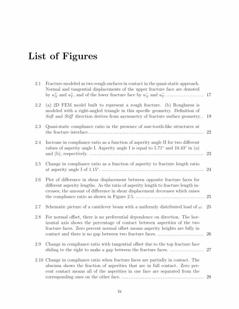
2.1 Fracture modeled as two rough surfaces in contact in the quasi-static approach.Normal and tangential displacements of the upper fracture face are denotedby u+

N and u+T , and of the lower fracture face by u−N and u−T . . . . . . . . . . . . . . . . . . . . . . 17

2.2 (a) 2D FEM model built to represent a rough fracture. (b) Roughness ismodeled with a right-angled triangle in this specific geometry. Definition ofSoft and Stiff direction derives from asymmetry of fracture surface geometry. . 19

2.3 Quasi-static compliance ratio in the presence of saw-tooth-like structures atthe fracture interface.. . . . . . . . . . . . . . . . . . . . . . . . . . . . . . . . . . . . . . . . . . . . . . . . . . . . . . . . . . . . . . . . 22

2.4 Increase in compliance ratio as a function of asperity angle II for two differentvalues of asperity angle I. Asperity angle I is equal to 5.71 and 10.43 in (a)and (b), respectively. . . . . . . . . . . . . . . . . . . . . . . . . . . . . . . . . . . . . . . . . . . . . . . . . . . . . . . . . . . . . . . . . 23

2.5 Change in compliance ratio as a function of asperity to fracture length ratioat asperity angle I of 1.15. . . . . . . . . . . . . . . . . . . . . . . . . . . . . . . . . . . . . . . . . . . . . . . . . . . . . . . . . . 24

2.6 Plot of difference in shear displacement between opposite fracture faces fordifferent asperity lengths. As the ratio of asperity length to fracture length in-creases, the amount of difference in shear displacement decreases which raisesthe compliance ratio as shown in Figure 2.5. . . . . . . . . . . . . . . . . . . . . . . . . . . . . . . . . . . . . . . 25

2.7 Schematic picture of a cantilever beam with a uniformly distributed load of ω. 25

2.8 For normal offset, there is no preferential dependence on direction. The hor-izontal axis shows the percentage of contact between asperities of the twofracture faces. Zero percent normal offset means asperity heights are fully incontact and there is no gap between two fracture faces. . . . . . . . . . . . . . . . . . . . . . . . . . . 26

2.9 Change in compliance ratio with tangential offset due to the top fracture facesliding to the right to make a gap between the fracture faces. . . . . . . . . . . . . . . . . . . . 27

2.10 Change in compliance ratio when fracture faces are partially in contact. Theabscissa shows the fraction of asperities that are in full contact. Zero per-cent contact means all of the asperities in one face are separated from thecorresponding ones on the other face. . . . . . . . . . . . . . . . . . . . . . . . . . . . . . . . . . . . . . . . . . . . . . . 28

ix

2.11 This figure shows how a waveform amplitude of a seismic wave is attenuatedby the presence of a smooth fracture. The solid line shows the amplitude ofa compressional seismic wave at the receiver in intact rock, while the dashedline is the waveform amplitude in the presence of a fracture. . . . . . . . . . . . . . . . . . . . . 30

2.12 Numerical results for dynamic measurements are compared with the singlecrack analytical solution presented in Equation (2.5). The dynamic compli-ance ratio increases slightly with an incremental increase in asperity angle. . . . . 31

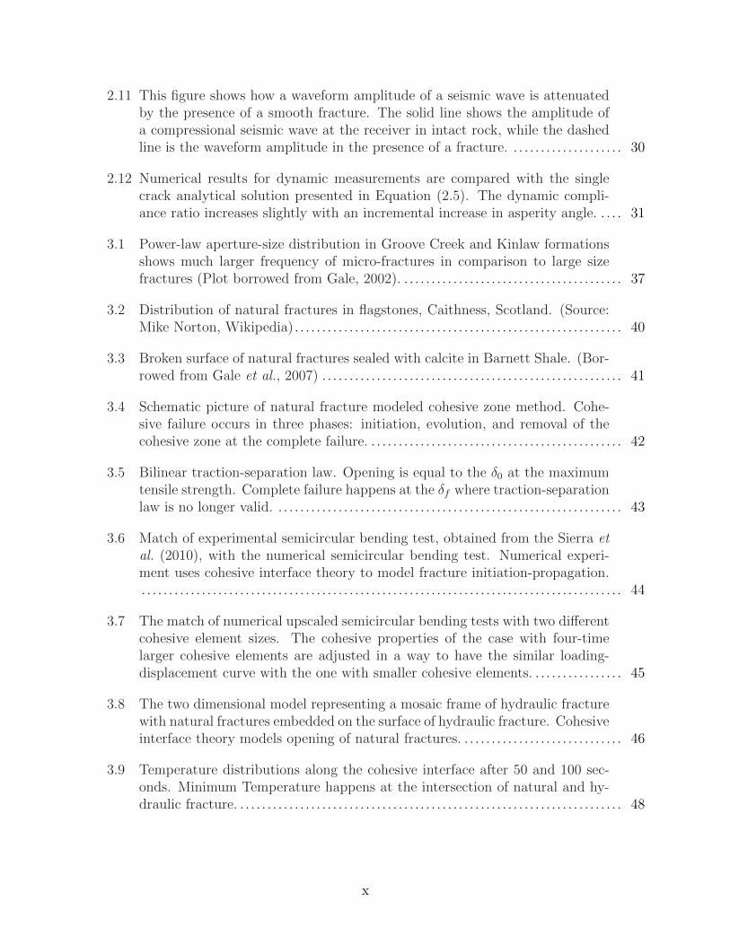
3.1 Power-law aperture-size distribution in Groove Creek and Kinlaw formationsshows much larger frequency of micro-fractures in comparison to large sizefractures (Plot borrowed from Gale, 2002). . . . . . . . . . . . . . . . . . . . . . . . . . . . . . . . . . . . . . . . . 37

3.2 Distribution of natural fractures in flagstones, Caithness, Scotland. (Source:Mike Norton, Wikipedia). . . . . . . . . . . . . . . . . . . . . . . . . . . . . . . . . . . . . . . . . . . . . . . . . . . . . . . . . . . . 40

3.3 Broken surface of natural fractures sealed with calcite in Barnett Shale. (Bor-rowed from Gale et al., 2007) . . . . . . . . . . . . . . . . . . . . . . . . . . . . . . . . . . . . . . . . . . . . . . . . . . . . . . . 41

3.4 Schematic picture of natural fracture modeled cohesive zone method. Cohe-sive failure occurs in three phases: initiation, evolution, and removal of thecohesive zone at the complete failure. . . . . . . . . . . . . . . . . . . . . . . . . . . . . . . . . . . . . . . . . . . . . . . 42

3.5 Bilinear traction-separation law. Opening is equal to the δ0 at the maximumtensile strength. Complete failure happens at the δf where traction-separationlaw is no longer valid. . . . . . . . . . . . . . . . . . . . . . . . . . . . . . . . . . . . . . . . . . . . . . . . . . . . . . . . . . . . . . . . 43

3.6 Match of experimental semicircular bending test, obtained from the Sierra etal. (2010), with the numerical semicircular bending test. Numerical experi-ment uses cohesive interface theory to model fracture initiation-propagation.. . . . . . . . . . . . . . . . . . . . . . . . . . . . . . . . . . . . . . . . . . . . . . . . . . . . . . . . . . . . . . . . . . . . . . . . . . . . . . . . . . . . . . . . 44

3.7 The match of numerical upscaled semicircular bending tests with two differentcohesive element sizes. The cohesive properties of the case with four-timelarger cohesive elements are adjusted in a way to have the similar loading-displacement curve with the one with smaller cohesive elements. . . . . . . . . . . . . . . . . 45

3.8 The two dimensional model representing a mosaic frame of hydraulic fracturewith natural fractures embedded on the surface of hydraulic fracture. Cohesiveinterface theory models opening of natural fractures. . . . . . . . . . . . . . . . . . . . . . . . . . . . . . 46

3.9 Temperature distributions along the cohesive interface after 50 and 100 sec-onds. Minimum Temperature happens at the intersection of natural and hy-draulic fracture. . . . . . . . . . . . . . . . . . . . . . . . . . . . . . . . . . . . . . . . . . . . . . . . . . . . . . . . . . . . . . . . . . . . . . . 48

x

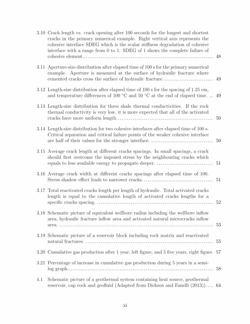
3.10 Crack length vs. crack opening after 100 seconds for the longest and shortestcracks in the primary numerical example. Right vertical axis represents thecohesive interface SDEG which is the scalar stiffness degradation of cohesiveinterface with a range from 0 to 1. SDEG of 1 shows the complete failure ofcohesive element.. . . . . . . . . . . . . . . . . . . . . . . . . . . . . . . . . . . . . . . . . . . . . . . . . . . . . . . . . . . . . . . . . . . . . 48

3.11 Aperture-size distribution after elapsed time of 100 s for the primary numericalexample. Aperture is measured at the surface of hydraulic fracture wherecemented cracks cross the surface of hydraulic fracture. . . . . . . . . . . . . . . . . . . . . . . . . . . 49

3.12 Length-size distribution after elapsed time of 100 s for the spacing of 1.25 cm,and temperature differences of 100 C and 50 C at the end of elapsed time. . . 49

3.13 Length-size distribution for three shale thermal conductivities. If the rockthermal conductivity is very low, it is more expected that all of the activatedcracks have more uniform length.. . . . . . . . . . . . . . . . . . . . . . . . . . . . . . . . . . . . . . . . . . . . . . . . . . . 50

3.14 Length-size distribution for two cohesive interfaces after elapsed time of 100 s.Critical separation and critical failure points of the weaker cohesive interfaceare half of their values for the stronger interface. . . . . . . . . . . . . . . . . . . . . . . . . . . . . . . . . . 50

3.15 Average crack length at different cracks spacings. In small spacings, a crackshould first overcome the imposed stress by the neighbouring cracks whichequals to less available energy to propagate deeper. . . . . . . . . . . . . . . . . . . . . . . . . . . . . . . 51

3.16 Average crack width at different cracks spacings after elapsed time of 100.Stress shadow effect leads to narrower cracks. . . . . . . . . . . . . . . . . . . . . . . . . . . . . . . . . . . . . . 51

3.17 Total reactivated cracks length per length of hydraulic. Total activated crackslength is equal to the cumulative length of activated cracks lengths for aspecific cracks spacing. . . . . . . . . . . . . . . . . . . . . . . . . . . . . . . . . . . . . . . . . . . . . . . . . . . . . . . . . . . . . . . 52

3.18 Schematic picture of equivalent wellbore radius including the wellbore inflowarea, hydraulic fracture inflow area and activated natural microcracks inflowarea. . . . . . . . . . . . . . . . . . . . . . . . . . . . . . . . . . . . . . . . . . . . . . . . . . . . . . . . . . . . . . . . . . . . . . . . . . . . . . . . . . . 53

3.19 Schematic picture of a reservoir block including rock matrix and reactivatednatural fractures. . . . . . . . . . . . . . . . . . . . . . . . . . . . . . . . . . . . . . . . . . . . . . . . . . . . . . . . . . . . . . . . . . . . . 55

3.20 Cumulative gas production after 1 year, left figure, and 5 five years, right figure. 57

3.21 Percentage of increase in cumulative gas production during 5 years in a semi-log graph.. . . . . . . . . . . . . . . . . . . . . . . . . . . . . . . . . . . . . . . . . . . . . . . . . . . . . . . . . . . . . . . . . . . . . . . . . . . . . 58

4.1 Schematic picture of a geothermal system containing heat source, geothermalreservoir, cap rock and geofluid (Adapted from Dickson and Fanelli (2013)). . . . 64

xi

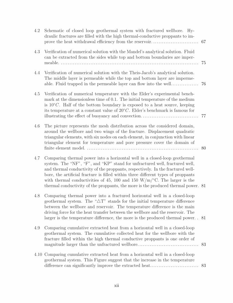
4.2 Schematic of closed loop geothermal system with fractured wellbore. Hy-draulic fractures are filled with the high thermal-conductive proppants to im-prove the heat withdrawal efficiency from the reservoir. . . . . . . . . . . . . . . . . . . . . . . . . . . 67

4.3 Verification of numerical solution with the Mandel’s analytical solution. Fluidcan be extracted from the sides while top and bottom boundaries are imper-meable. . . . . . . . . . . . . . . . . . . . . . . . . . . . . . . . . . . . . . . . . . . . . . . . . . . . . . . . . . . . . . . . . . . . . . . . . . . . . . . . 75

4.4 Verification of numerical solution with the Theis-Jacob’s analytical solution.The middle layer is permeable while the top and bottom layer are imperme-able. Fluid trapped in the permeable layer can flow into the well.. . . . . . . . . . . . . . . 76

4.5 Verification of numerical temperature with the Elder’s experimental bench-mark at the dimensionless time of 0.1. The initial temperature of the mediumis 10C. Half of the bottom boundary is exposed to a heat source, keepingits temperature at a constant value of 20C. Elder’s benchmark is famous forillustrating the effect of buoyancy and convection. . . . . . . . . . . . . . . . . . . . . . . . . . . . . . . . . 77

4.6 The picture represents the mesh distribution across the considered domain,around the wellbore and two wings of the fracture. Displacement quadratictriangular elements, with six nodes on each element, in conjunction with lineartriangular element for temperature and pore pressure cover the domain offinite element model. . . . . . . . . . . . . . . . . . . . . . . . . . . . . . . . . . . . . . . . . . . . . . . . . . . . . . . . . . . . . . . . . 80

4.7 Comparing thermal power into a horizontal well in a closed-loop geothermalsystem. The “NF”, “F”, and “KP” stand for unfractured well, fractured well,and thermal conductivity of the proppants, respectively. In the fractured well-bore, the artificial fracture is filled within three different types of proppantswith thermal conductivities of 45, 100 and 150 W/m/C. The larger is thethermal conductivity of the proppants, the more is the produced thermal power. 81

4.8 Comparing thermal power into a fractured horizontal well in a closed-loopgeothermal system. The “4T” stands for the initial temperature differencebetween the wellbore and reservoir. The temperature difference is the maindriving force for the heat transfer between the wellbore and the reservoir. Thelarger is the temperature difference, the more is the produced thermal power. . 81

4.9 Comparing cumulative extracted heat from a horizontal well in a closed-loopgeothermal system. The cumulative collected heat for the wellbore with thefracture filled within the high thermal conductive proppants is one order ofmagnitude larger than the unfractured wellbore. . . . . . . . . . . . . . . . . . . . . . . . . . . . . . . . . . . 83

4.10 Comparing cumulative extracted heat from a horizontal well in a closed-loopgeothermal system. This Figure suggest that the increase in the temperaturedifference can significantly improve the extracted heat.. . . . . . . . . . . . . . . . . . . . . . . . . . . 83

xii

4.11 Temperature drop, in centigrade, across the geothermal model after 20 yearsof heat withdrawal. Temperature drop is calculated by subtraction of thecurrent temperature from the initial temperature. . . . . . . . . . . . . . . . . . . . . . . . . . . . . . . . . 85

4.12 Temperature drop changes versus time, measured along one of the fracturewings. Fracture is filled by the proppants with thermal conductivity of 150W/m/C. The initial temperature gradient at the wellbore is 100C. . . . . . . . . . . . 85

4.13 Pressure drop, in Pa, across the geothermal model after 20 years of heat with-drawal. Pressure drop is calculated by subtraction of the current temperaturefrom the initial temperature.. . . . . . . . . . . . . . . . . . . . . . . . . . . . . . . . . . . . . . . . . . . . . . . . . . . . . . . . 86

4.14 Horizontal displacement, in meter, across the geothermal model after 20 yearsof heat withdrawal. The maximum horizontal displacement happens aroundthe wellbore. . . . . . . . . . . . . . . . . . . . . . . . . . . . . . . . . . . . . . . . . . . . . . . . . . . . . . . . . . . . . . . . . . . . . . . . . . 87

4.15 Vertical displacement, in meter, across the geothermal model after 20 yearsof heat extraction. The maximum vertical displacement happens around thewellbore. . . . . . . . . . . . . . . . . . . . . . . . . . . . . . . . . . . . . . . . . . . . . . . . . . . . . . . . . . . . . . . . . . . . . . . . . . . . . . . 87

4.16 Surface subsidence versus time in a closed-loop fractured wellbore. The mag-nitude of surface subsidence increases with time. The largest subsidence hap-pens at the middle of the model where the horizontal well is intersected witha vertical fracture. . . . . . . . . . . . . . . . . . . . . . . . . . . . . . . . . . . . . . . . . . . . . . . . . . . . . . . . . . . . . . . . . . . . 88

4.17 Principal horizontal stress across the geothermal model after 20 years of heatextraction. The stress unit is Pa. . . . . . . . . . . . . . . . . . . . . . . . . . . . . . . . . . . . . . . . . . . . . . . . . . . . 89

4.18 Principal vertical stress across the geothermal model after 20 years of heatextraction. The stress unit is Pa. . . . . . . . . . . . . . . . . . . . . . . . . . . . . . . . . . . . . . . . . . . . . . . . . . . . 89

4.19 Shear stress across the geothermal model after 20 years of heat extraction.The stress unit is Pa. . . . . . . . . . . . . . . . . . . . . . . . . . . . . . . . . . . . . . . . . . . . . . . . . . . . . . . . . . . . . . . . . 90

xiii

Abstract

Fractures are a source of extra compliance in the rock mass. Fracture compliance can es-

timate the fracture roughness and the type of fluid filling the fracture. The focus of this

research study in chapter 2 is to illustrate how the compliance ratio of rough fractures can di-

verge from the compliance ratio of smooth fractures. The imperfect interface of the fracture

is modeled with saw-tooth-like structures. The defined saw-tooth-like structures of contact

asperities impose an in-plane asymmetry in the shear direction. The compliance ratio of the

rough fracture is larger than the compliance ratio of the smooth fracture. Interlocking and

riding up effects may explain our findings in chapter 2.

Recovered core samples and extensive outcrops studies have proved the existence of natu-

ral fractures in many tight formations. These natural fractures are likely filled with digenetic

materials such as clays, quartz or calcite. In chapter 3, this study suggests that small ce-

mented natural fractures can be opened by the induced tensile stress due to the temperature

difference between the cold fracturing fluid and hot formation. Cohesive zone model (CZM)

is utilized here to simulate these natural fractures. Contribution of these micro natural frac-

tures to cumulative gas production from a shale reservoir is investigated by modifying the

transmissibility coefficient. Reservoir simulation results in chapter 3 suggest that reactivated

natural fractures in the tight formations at early stages can improve gas production up to

25%; however, their effect significantly reduces to 3% in long term.

Geothermal systems are identified as either open-loop systems (OLGS) or closed-loop

systems (CLGS). The loss of working fluid, surface subsidence, formation compaction, and

xiv

induced seismicity are major challenges in OLGS. To address the indicated challenges, CLGS

can be considered as an alternative option. To improve the heat extraction from closed-

loop wells, this research study in chapter 4 suggests highly conductive hydraulic fractures

for CLGS to improve heat extraction rate. The results suggest that fractures significantly

improve thermal power and cumulative extracted heat in CLGS. Thermal conductivity of

the proppants is the key parameter enhancing heat extraction.

xv

Chapter 1Overview

1.1 Introduction

Hydraulic fracturing has been recognized as the most effective technique for economic recov-

ery in tight oil and gas formations in North America (Holditch, 2006; Moniz et al., 2006).

Induced fractures significantly improve wellbore-formation contact area by creating a highly

permeable conduit in the reservoir. The direction of hydraulic fracture propagation depends

on the direction of the minimum principal stress as well as natural fractures (Economides

and Nolte, 2000; Dahi Taleghani and Olson, 2011). Natural fractures are mechanical dis-

continuities in rock with the lengths varying from micrometers to kilometers (Narr et al.,

2006). These fractures can be formed due to tectonic deformation, excessive pore pressure, or

major temperature change. Core and outcrop studies, advanced logging tools, microseismic

techniques and well testing analysis have proved the existence of natural fractures in many

unconventional reservoirs. Due to the limited access to the subsurface and limited precision

of seismic techniques, outcrops are the main source to speculate fracture’s geometry in the

subsurface. Existence of natural fractures in the outcrop samples could be an indicative of

their existence in the subsurface. However, most of the outcrop studies are qualitative and

the existing models studying the interaction of natural fractures with the hydraulic fracture

mainly consider the contribution of large natural fractures. Large natural fractures are the

ones with the dimensions comparable to the size of hydraulic fracture (Jeffrey et al., 2009;

Dahi Taleghani and Olson, 2014).

1

Naturally fractured reservoirs frequently exhibit anisotropy in permeability, geomechan-

ical properties and seismic velocities as they exist in one or more sets of partially aligned

series. This anisotropy makes the prediction of reservoir performance more difficult. In the

reservoirs with low-matrix permeability, fractures act as the primary conduits for fluid flow,

whereas in reservoirs with higher permeability, they act as shortcuts for fluid flow. Con-

tribution of natural fractures in the hydrocarbon recovery is more significant in the tight

formations with low permeability than permeable reservoirs. However, they can also increase

the leak-off volume during the fracturing treatments leading to early screenouts or poorly

propped hydraulic fractures. Inaccurate evaluation of natural fractures not only affects the

performance of waterflooding projects leading to low sweep efficiency, but also causes poor

drilling performance resulting from lost circulation (Narr et al., 2006). Knowledge of the

orientation and density of fractures in the subsurface are thus important for designing well

layout for optimal production and choosing an appropriate EOR technique (Reiss, 1980; Nel-

son, 2001; Saidi, 1987). Arrest and diversion of hydraulic fracture front into the pre-existing

natural fractures have been the subject of many experimental and theoretical studies (Gon-

zalez et al., 2015).

In reality, fracture faces are not smooth and instead consist of the asperities and mor-

phological irregularities (Nagy, 1992; Yoshioka and Scholz, 1989b). These asperities are

generally aligned perpendicular to the direction of the crack propagation or the direction of

the fluid flow in the sedimentary rocks (Aydan et al., 1996). The distribution and height of

these ridges depend on the direction of the fracture slippage, rate of the slippage and the

magnitude of the shearing stress (Durney and Ramsay, 1973). Degree of contact between

fracture faces controls both fracture mechanical and hydromechanical properties. For in-

stance, fracture ability to allow the fluid flow and to conduct the electrical current depends

on the degree of contact between the fracture faces (Brown, 1989). Fracture compliance

can be used to estimate the degree of fracturing of the rock mass, type of fluid filling the

fracture and fracture roughness (Verdon and Wstefeld, 2013; Yoshioka and Scholz, 1989a).

2

Assessing the ratio of normal to tangential compliance may help in reservoir characteriza-

tion, because compliance ratio depends on the type of material filling the fracture, such as

clay or cement between the fracture faces, or fluid saturating the fracture, and the degree of

fracture roughness. In Chapter 2, this research study uses the finite-element method (FEM)

to investigate the effects of surface asperities and fracture offset on the fracture compliance

ratio. To characterize the geometry of the fracture interface, we model fracture faces as pe-

riodic saw-tooth-like structures in a Cartesian system. The idea of such a specific geometry

is inspired by Aydan et al. (1996), who reported saw-tooth-like structures at the fracture

interface of sheeting joints in granite.

Field studies have confirmed the existence of a critical threshold that cracks with aperture

less than this threshold are fully filled with digenetic materials (Laubach, 200). Laboratory

measurements have proved that these filled natural fractures may act as the weak path for

rock failure. For instance in Barnett shale samples,tensile strength of cemented cracks can be

about 10 times lower than the tensile strength of intact rocks (Gale et al., 2007). Power-law

distribution of natural fractures indicate that small-size fractures are orders of magnitudes

more than the large-size fractures in the tight formations. Therefore, it is not surprising if

the induced hydraulic fractures are intersecting thousands of these small-fractures. Since the

small-size natural fractures exist in large numbers, only partial reactivation of these fractures

may affect fluid flow in the vicinity of the hydraulic fracture. This effect could be positive

by enhancing the permeability around the fracture and improving hydrocarbon production,

or could be negative by increasing the leak-off volume and boosting the capillary trapping.

The entrapped water, which is essentially part of the leak-off volume that will never produce,

could hinder hydrocarbon flow from the formation into the hydraulic fracture. Low required

energy for the reactivation of small natural fractures makes them easy targets for reopening

if large enough tensile stress is available at the surface of hydraulic fracture. Parameters

controlling the opening of these small fractures are the tensile strength of cementing materials

filling the fractures, magnitude of the tensile stress, and fractures density.

3

Fracturing fluid is frequently pumped with the temperature close to the surface temper-

ature; therefore, its temperature at the bottomhole usually differs from the reservoir tem-

perature, especially in deep and hot formations. Temperature of fracturing fluid delivered

at the surface of hydraulic fracture depends on the injection rate, casing/tubing diameter,

heat capacity of fracturing fluid, and fracture width. Temperature difference between cold

fracturing fluid and hot reservoir rock induces tensile stress at the surface of hydraulic frac-

ture. Magnitude of induced thermal stress is not large enough to induce large cracking in the

rock, but it may be sufficient for opening of small-size natural fractures filled with the dige-

netic materials since they are weaker than the intact rock. In chapter 3, this study aims to

quantitatively estimate the opening of small pre-existing natural fractures, activated by the

induced thermal stress between the hot formation and cold fracturing fluid, and show their

contribution in the hydrocarbon recovery. Sensitivity analysis on the parameters controlling

reactivation of pre-existing natural fractures is examined to determine the significance of

each parameter on the opening of natural fractures.

Drastic climate changes during the last century caused by the emission of greenhouse

gases from the burning fossil fuels has encouraged countries to expand the application of

clean and sustainable energy resources. Geothermal energy is one of these sustainable re-

sources and the general interest in the production of electricity from the geothermal power

plants has immensely risen in recent years. Hot dry rocks are one of the common geothermal

resources in the world. In these reservoirs, there is not enough fluid in place to be used for the

heat extraction. Lack of fluid in place in the hot dry rock reservoirs may have a significant

drawback. To overcome this problem, a working fluid should be injected into the reservoir

to absorb the heat, and later be produced from production wells. In this system, enough

reservoir permeability is crucial for the project success. In a reservoir with low permeabil-

ity, hydraulic fracturing treatments are performed to increase injectivity and productivity.

The amount of the produced heat in this system depends on the rock temperature, rate

of fluid circulation in the reservoir, and the swept volume by the injected working fluid.

4

Loss of the working fluid, affecting total cost of the produced electricity, is a common issue.

However, drawbacks are not limited to only this issue. Surface subsidence, formation com-

paction, induced earthquakes, and consequent damages to the wellbore integrity are other

disadvantages of heat extraction from open-loop systems (Majer et al., 2007).

To address the indicated issues, closed-loop geothermal system can be considered as an

alternative solution. In this method, a working fluid, with low-boiling point, is circulated

inside a series of coaxial sealed pipes to extract the stored heat in the reservoir. The low-

boiling point improves the heat extraction efficiency (Diao et al., 2004). It is expected

that the lack of fluid production/injection from/into the reservoir should not significantly

affect the pore pressure distribution. The closed-loop system has negligible environmental

hazard compared to the open-loop system. For instance, produced water in an open-loop

system contains high levels of sulfur, salt, and radioactive elements. Therefore, extracted

water should be injected back into the reservoir which is a costly process (Kagel et al.,

2005). Land subsidence is another drawback in the open-loop systems. Production of the

ground water reduces the pore pressure. Most of the open-loop facilities address this problem

with reinjection of the produced fluid into the reservoir; however, this solution can induce

significant seismic events. For instance, induced earthquakes in an open-loop geothermal

plant in Basel, Switzerland, led to suspension of the whole project (Giardini, 2009). In

chapter 4, focus of the research study is on enhancing heat extraction from a closed-loop

geothermal wellbore via thermal conductive fractures. A thermoporoelastic finite element

model is developed to study the geomechanical behavior of the proposed system as well as

heat production. Thermoporoelasticity enables us to couple temperature, pore pressure, and

displacement changes in the reservoir especially close to the wellbore. To solve the governing

partial equations, Finite Element Method (FEM) is used to solve the governing equations.

5

1.2 Research Objectives

The proposed research has the following objectives:

Investigate the effects of surface asperities and fracture offset on the fracture compli-

ance ratio. Presence of fractures in a rock medium makes the medium more compliant.

The magnitude of this additional compliance depends on various parameters such as

fracture roughness, type of the fluid filling the fracture, fluid viscosity, rock permeabil-

ity, fracture connectivity and the presence of cement, clay and other fracture fillings.

In this research study, fracture rough interface is modeled with periodic saw-tooth-like

structures in a Cartesian system. This research proposal studies different geometrical

and offset configurations to show how compliance ratio is a function of available contact

area at the fracture interface and also the size of the asperities.

To quantitatively estimate the opening of small pre-existing natural fractures, acti-

vated by the induced thermal stress between the hot formation and cold fracturing

fluid, and show their contribution in the hydrocarbon recovery. Cohesive zone model

(CZM) is utilized here to simulate these natural fractures. Tensile strength of digenetic

cements, temperature difference between the fracturing fluid and formation, fractures

spacing, and rock conductivity are the parameters controlling the opening and length

of reactivated micro-fractures. Sensitivity analysis on these parameters is examined to

determine the significance of each parameter on the opening of natural fractures.

To provide a comprehensive analysis of a new method for heat extraction from the

low-enthalpy geothermal reservoirs without mass withdrawal. The developed coupled

numerical model in this study assesses the effectiveness of the proposed closed-loop

configuration including the induced hydraulic fractures propped with highly thermal

conductive materials to enhance heat production. Closed-loop geothermal system can

be considered as an alternative solution for the open-loop systems. The level of surface

6

subsidence and seismic risk assessment in the proposed technique is also measured to

investigate the safety and environmental hazards of proposed technique.

1.3 References

Aydan, O., Y. Shimizu, and T. Kawamoto. “The anisotropy of surface morphology and shearstrength characteristics of rock discontinuities and its evaluation.” NARMS 96 (1996):1391-1398.

Brown, S. R. “Transport of fluid and electric current through a single fracture.” Journal ofGeophysical Research: Solid Earth 94, no. B7 (1989): 9429-9438.

Bonnet, E., O. Bour, N. E. Odling, P. Davy, I. Main, P. Cowie, and B. Berkowitz. “Scalingof fracture systems in geological media.” Reviews of geophysics 39, no. 3 (2001): 347-383.

Diao, N., Q. Li, and Z. Fang. “Heat transfer in ground heat exchangers with groundwateradvection.” International Journal of Thermal Sciences 43.12 (2004): 1203-1211.

Dahi Taleghani, A., and J. Olson. “Numerical modeling of multistranded-hydraulic-fracturepropagation: accounting for the interaction between induced and natural fractures.” SPEJournal 16.3 (2011): 575-581.

Dahi Taleghani, A., and J. E. Olson. “How natural fractures could affect hydraulic-fracturegeometry.” SPE Journal 19, no. 01 (2014): 161-171.

Durney, D. W, and J. G. Ramsay. “Incremental strains measured by syntectonic crystalgrowths.” Gravity and tectonics 67 (1973): 96.

Economides, M. J. and K.G. Nolte. “Reservoir stimulation.” Wiley Press, 2000.

Gale, J. FW, R. M. Reed, and J. Holder. “Natural fractures in the Barnett Shale and theirimportance for hydraulic fracture treatments.” AAPG bulletin 91, no. 4 (2007): 603-622.

Giardini, D. “Geothermal quake risks must be faced” Nature 462.7275 (2009): 848-849.

Gonzalez-Chavez, M., P. Puyang, and A. D. Taleghani. “From semi-circular bending testto microseismic maps: an integrated modeling approach to incorporate natural fractureeffects on hydraulic fracturing.” Unconventional resources technology conference, SPE.Aug. 2015.

Holditch, S. A. “Tight gas sands.” Journal of Petroleum Technology 58, no. 06 (2006): 86-93.

Jeffrey, R., X. Zhang, and M. Thiercelin. ”Hydraulic Fracture Offsetting in Naturally Frac-tures Reservoirs: Quantifying a Long-Recognized Process.” SPE Hydraulic FracturingTechnology Conference. 2009.

Kagel, A., D. Bates, and K. Gawell. “A guide to geothermal energy and the environmentWashington, DC: Geothermal Energy Association, (2005).

7

Laubach, S. E. ”Practical approaches to identifying sealed and open fractures.” AAPG bul-letin 87, no. 4 (2003): 561-579.

Majer, E. L., R. Baria, M. Stark, S. Oates, J. Bommer, B. Smith, and H. Asanuma. “Inducedseismicity associated with enhanced geothermal systems” Geothermics 36.3 (2007): 185-222.

Moniz, E. J., H. D. Jacoby, A. J. M. Meggs, R. C. Armtrong, D. R. Cohn, S. R. Connors,J. M. Deutch, Q. J. Ejaz, J. S. Hezir, and G. M. Kaufman. “The future of natural gas.”Cambridge, MA: Massachusetts Institute of Technology (2011).

Nagy, P. B. “Ultrasonic classification of imperfect interfaces.” Journal of Nondestructiveevaluation 11, no. 3-4 (1992): 127-139.

Narr, W., D. W. Schechter, and L. B. “Thompson. Naturally fractured reservoir characteri-zation.” Richardson, TX: Society of Petroleum Engineers, 2006.

Nelson, R. “Geologic analysis of naturally fractured reservoirs.” Gulf Professional Publishing,2001.

Potluri, N. K., D. Zhu, and A. D. Hill. “The effect of natural fractures on hydraulic fracturepropagation.” In SPE European Formation Damage Conference. Society of PetroleumEngineers, 2005.

Reiss, L. H. “The reservoir engineering aspects of fractured formations”. Vol. 3. EditionsTechnip, 1980.

Saidi, A. M. “Reservoir Engineering of Fractured Reservoirs (fundamental and PracticalAspects).” Total, 1987.

Verdon, J. P., and A. Wstefeld. “Measurement of the normal/tangential fracture compli-ance ratio (ZN/ZT) during hydraulic fracture stimulation using Swave splitting data.”Geophysical Prospecting 61, no. s1 (2013): 461-475.

Warpinski, N. R., and L. W. Teufel. “Influence of geologic discontinuities on hydraulic frac-ture propagation.” Journal of Petroleum Technology 39, no. 02 (1987): 209-220.

Yoshioka, N., and Ch. H. Scholz. “Elastic properties of contacting surfaces under normal andshear loads, 1, Theory.” Journal of Geophysics. Res 94, no. B12 (1989): 17681-17690.

Yoshioka, N., and Ch. H. Scholz. “Elastic properties of contacting surfaces under normal andshear loads: 2. Comparison of theory with experiment.” Journal of Geophysical Research:Solid Earth 94, no. B12 (1989): 17691-17700.

8

Chapter 2Effects of Roughness and Offset on Frac-ture Compliance Ratio*

2.1 Introduction

Significant percentage of hydrocarbon reservoirs are naturally fractured while some of these

reservoirs have low permeability (Reiss, 1980; Nelson, 2001). Economic oil or gas produc-

tion from these reservoirs depends on the connectivity of natural fractures network and

execution of hydraulic fracturing treatments. Fractures can be defined as discontinuities in

rock caused by tectonic deformation, excessive pore pressure, or major temperature change.

Natural fractures may act as shortcuts or preferential flow paths for reservoir fluid recov-

ery. Because fractures in hydrocarbon reservoirs often exist in one or more sets of partially

aligned fractures, naturally fractured reservoirs frequently exhibit anisotropy in permeabil-

ity, geomechanical properties and seismic velocities. This anisotropy makes the prediction

of reservoir performance more difficult (Bedayat and Dahi Taleghani, 2016). Consequently,

characterizing natural fractures in the subsurface is essential. The inaccurate evaluation of

natural fractures not only affects the performance of waterflooding projects leading to low

sweep efficiency, but also causes poor drilling performance resulting from lost circulation

(Narr et al., 2006).

*Part of this chapter 2 previously appeared as ”Ahmadi, M., A. Dahi Taleghani, and C. M. Sayers.The Effects of Roughness and Offset on Fracture Compliance Ratio. Geophysical Journal International(2016) 205 (1): 454-463” and ”Ahmadi, M., A. Dahi Taleghani, and C. M. Sayers. Direction Dependence ofFracture Compliance Induced by Slickensides. Geophysics (2014) 79 (4): C91-C96”. There are reprinted bypermission of Oxford University Press and Society of Exploration Geophysicists (Appendix C).

9

In reality, fracture faces are not smooth and instead have rough-walled structures (Yosh-

ioka and Scholz, 1989a; Yoshioka and Scholz, 1989b; Nagy, 1992). Fracture faces consist of

the asperities and morphological irregularities. These asperities are generally aligned per-

pendicular to the direction of the crack propagation or the direction of the fluid flow in the

sedimentary rocks (Paterson, 1958; Aydan et al., 1996). The distribution and height of these

ridges depend on the direction of the fracture slippage, rate of the slippage and the magni-

tude of the shearing stress (Durney and Ramsay, 1973). Aydan et al. (1996) suggested that

the fracture discontinuities have different shear strengths in the different shear directions.

The degree of contact between fracture faces controls both fracture mechanical and hy-

dromechanical properties. For instance, fracture ability to allow the fluid flow and to conduct

electrical current depends on the degree of contact between the fracture faces (Brown, 1989).

Fracture roughness and fracture aperture control fluid flow and proppant delivery during hy-

draulic fracturing treatments (Van Dam and de Pater, 1999). Liu (2005) discussed how

the roughness affects the fracture mechanical and hydraulic apertures and if the mechanical

aperture is at the same scale as the surface roughness, it is no longer realistic to assume that

the mechanical and hydraulic apertures are equal, requiring correction in the fracture aper-

ture estimated from the seismic data to be further used in reservoir simulations. Fracture

roughness is scale dependent. In other words, the observed distribution of roughness signifi-

cantly depends on the considered wavelength (Power et al., 1988; Sagy et al., 2007; Candela

et al., 2009). Root mean square (rms), joint roughness coefficient, height of roughness, max-

imumminimum height difference, Fourier power spectrum and wavelet power spectrum are

some of the processing techniques used to quantify roughness and structure of the fracture

asperities (Sagy et al., 2007; Candela et al., 2009).

There are several methods for predicting, evaluating and characterizing natural fractures

in the subsurface, including analysis of core samples, well-logging techniques and seismic

methods (Laubach et al., 2000; Liu, 2005; Gale et al., 2007; Olson et al., 2009). Comprehen-

sive knowledge of natural fractures (fracture orientation, spacing and spatial distribution)

10

can tremendously improve the well-layout design to maximize the likelihood of intersect-

ing natural fractures, and can greatly enhance hydrocarbon production in low-permeability

reservoirs. Although fracture data obtained from core analysis and borehole imaging are very

useful to understand the existence of fractures in the subsurface, these data do not provide

information between the wells. Therefore, other measurements, such as seismic velocity and

amplitude, are required to characterize fracture density and orientation away from the wells

(Sayers, 2009; Bachrach, 2013). Fracture size, orientation and density can be estimated from

seismic data (Liu et al., 2003; Maultzsch et al., 2003). Seismic wave velocities, amplitudes

and spectral characteristics can be distorted by the presence of fractures. This distortion

can be used to further estimate fracture compliance, and can improve our knowledge about

the fractured reservoir in order to better predict its behavior and design better depletion

strategies.

The velocity of seismic waves in the subsurface significantly depends on rock type, stress

state, pore pressure, fluid type and the presence or absence of natural fractures. Fractures can

change both compressional and shear wave velocities. The variation of seismic wave velocities

through the formation is sensitive to fracture properties such as fracture orientation, spacing,

aperture, length, saturation and the presence or absence of cement, clay and other types of

fracture fill (Sayers and Kachanov, 1991; Sayers and Kachanov, 1995; Schoenberg and Sayers,

1995; Boadu and Long, 1996; Leucci and De Giorgi, 2006; Lubbe et al., 2008).

Fracture compliance can be used to estimate the degree of fracturing of the rock mass,

type of fluid filling the fracture and fracture roughness (Schoenberg and Sayers, 1995; Yosh-

ioka and Scholz, 1989a; Lubbe et al., 2008; Verdon and Wustefeld, 2013; Ahmadi et al., 2014;

Rubino et al., 2014). Fracture compliance can be represented as a second-rank tensor, with

normal and shear components. Assessing the ratio of normal to tangential compliance may

help in reservoir characterization, because compliance ratio depends on the type of material

filling the fracture, such as clay or cement between the fracture faces (Sayers et al., 2009),

or fluid saturating the fracture, and the degree of fracture roughness. In this study, we aim

11

to show how compliance ratio can be affected by rough interface contact area. We calcu-

late the compliance ratio using two different approaches: quasi-static and dynamic. In the

quasi-static method, we calculate compliance from the jump in the displacement across the

fracture interface divided by applied stress. However, in the dynamic technique, we calcu-

late transmission coefficient as the ratio of waveform peak amplitudes to estimate compliance

ratio.

2.2 Determination of Fracture Compliance

Fracture compliance depends on the mechanical properties of the fracture network and host

rock, structure of fracture roughness and degree of cementation or mineralization on the

fracture faces (Lubbe et al., 2008; Sayers et al., 2009; Rubino et al., 2014). Fracture com-

pliance can have applications in different fields, such as rock damage and stability analysis,

hydrocarbon recovery, hydraulic fracturing, disposal of nuclear wastes, fault slippage and

laboratory nondestructive tests (Mollhoff et al., 2010). In fractures with the ability of fluid

exchange via small pathways, Hudson et al. (1996) suggest that for a random distribution of

coplanar cracks in an infinite domain, the ratioBN

BT

of the normal compliance BN to shear

compliance BT is

BN

BT

=(1 + A)(1− ν

2)

1 +B(2.1)

where

A =4a

πc(iωηfµ

)(1− ν2− ν

) (2.2)

and

B = [2a

πc

κfµ

(1− ν)](1− 3iκfk2Kr

4πνa2cωηf)−1 (2.3)

12

Here, µ and ν are the shear modulus and Poisson’s ratio of the solid matrix, κf and ηf

are the bulk modulus and viscosity of the fluid, respectively,c

ais the aspect ratio of the

fractures, ω is the angular frequency, k is the wavenumber and Kr is the permeability of the

rock medium including the contribution of cracks and cavities in permeability enhancement.

In fractured reservoirs with very low permeability, the compliance ratio in Equation (2.1)

simplifies to

BN

BT

=(1 + A)(1− ν

2)

1 +2a

πc

κfµ

(1− ν)(2.4)

An increase in the bulk modulus of the fluid leads to a decrease in compliance ratio.

Moreover, the saturation of fractures with intrinsic fluid affects compliance ratio because

effective bulk modulus is a function of fluid saturation. For instance, compliance ratio in

a fractured rock saturated with gas is larger than that of a water saturated rock (Sayers

and Kachanov, 1995; Hobday and Worthington, 2012; Verdon and Wustefeld, 2013). A

simplified version of Equation (2.4) for the case of a dry or gas-filled fracture within rough

faces is shown in Equation (2.5):

BN

BT

=1− ν1− ν

2

(2.5)

None of the mentioned models consider the effect of diagenesis or contact points along the

fracture length. In the proposed formulae, fracture surfaces are considered as two separated

faces with no welding, cementation, or interaction with each other. In particular, fracture

faces do not have any relative shear strength against sliding induced by interface roughness

or the presence of asperities. Resistance against sliding generally depends on roughness,

bridging,cementation and contact areas between fracture faces.

Fracture compliance can be measured using either a quasi-static or dynamic technique

(Pyrak-Nolte et al., 1987; Pyrak-Nolte et al., 1990; Barton, 2007). Quasi-static compliance

13

is measured at zero frequency; however, dynamic compliance corresponds to finite frequency.

Pyrak-Nolte et al. (1987) and Pyrak-Nolte et al. (1990), through ultrasonic laboratory exper-

iments, showed quasi-static normal compliance in quartz monzonite samples is larger than

dynamic normal compliance in the same rock sample. The magnitude of the discrepancy in

normal compliance between these techniques rises as the applied compressive stress on the

sample increases. Friction is considered to be one of the causes of this discrepancy. However,

another possibility for this discrepancy can be related to the difference in the magnitude of

strain amplitudes in quasi-static and dynamic laboratory experiments. Strain amplitude in

dynamic measurements is much smaller than in static measurements. The amplitude of elas-

ticwaves is too small to trigger sliding of fracture faces; therefore, displacement magnitude

may be the dominant cause of the difference between the static and dynamic measurements.

From a field study on water-saturated fractures at the north coast of Scotland, Hobday and

Worthington (2012) concluded that the compliance ratio of saturated fractured rocks in this

region is less than 0.1. This low value of compliance ratio is what they attribute it to the

presence of water contained in the fractures. They suggested that partially air-saturated

fractures can have larger compliance ratio values; however, they could not characterize or

recognize them in that specific area. MacBeth and Schuett (2007) studied the effect of di-

agenesis on the compliance of natural micro-fractures. They concluded that diagenesis can

decrease compliance ratio by increasing the contact area between fracture faces.

One important potential application of the compliance ratio measurement has been stud-

ied by Verdon and Wustefeld (2013). Using the S-wave splitting technique, they monitored

the progress of a hydraulic fracturing treatment in the Cotton Valley tight gas reservoir

in Texas. They reported notable fluctuations in compliance ratio during different stages of

hydraulic fracturing stimulation. They showed that proppant injection increases compliance

ratio up to a value of two, which is more than the analytical value of 1 for the compliance

ratio of a single fracture in 2D. They concluded that this discrepancy can be caused by the

generation of new fractures or the activation of pre-existing fractures around the main hy-

14

draulic fracture. In this research study, we will see that this effect can be related to slippage

along the fracture that can also occur at the intersection with natural fractures.

In this study, we calculate the compliance ratio of a single fracture and show how the

presence of offset or roughness on the fracture face affects compliance ratio. Fractures are

considered as discontinuities in which stress is continuous along the fracture faces, but dis-

placement may be discontinuous. Any incremental change in the stress field around the

fracture produces a linear incremental change in the displacement across the fracture faces.

This excess displacement is characterized by the fracture compliance. To calculate the ex-

cess displacement in our calculations in the quasi-static technique, a pair of points at the

center of fracture, one at the top face and one at the bottom face, is selected when the whole

system is in the initial equilibrium and no normal or tangential stress is applied. These two

points initially have the same coordinates as the top point lay down on the bottom point.

A 2D crack in an infinite medium, subjected to stress at infinity, has a compliance ratio

of 1. In the quasi-static approach, compliance is determined as the ratio of the difference

between the displacement of fractured rock and the displacement in intact rock divided by

the applied stress applied at the infinite boundary. The calculation of compliance from the

dynamic technique is explained in the following section.

2.3 Dynamic Technique to Measure Fracture Compliance

Schoenberg (1980) derived an analytical solution for an imperfectly bonded interface in an

isotropic, linear elastic medium, known as linear-slip theory. He assumed a harmonic wave of

angular frequency ω and unit amplitude passed through the fractured medium. In this model,

stress along the fracture is continuous but displacement may be discontinuous. Reflection (R)

and transmission (T ) coefficients of a harmonic plane wave, with angular frequency ω, across

the imperfectly bonded interface are computed from interface compliances. In a homogenous

15

elastic medium with a discontinuity, reflection (R) and transmission (T ) coefficients are:

R(ω) =iωρV B

2 + iωρV B(2.6)

and

T (ω) =2

2 + iωρV B(2.7)

where ρ is rock density, ω is angular frequency, V is wave velocity and B is fracture com-

pliance. For a compressional wave, V and B are equal to the compressional wave velocity

and normal compliance. For a shear wave, V and B are the shear wave velocity and shear

compliance.

There are differences in the amplitudes of seismic compressional and shear waves between

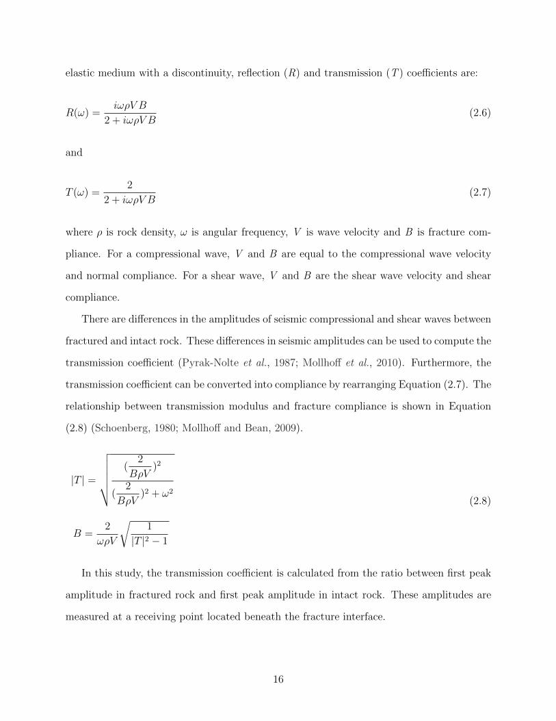
fractured and intact rock. These differences in seismic amplitudes can be used to compute the

transmission coefficient (Pyrak-Nolte et al., 1987; Mollhoff et al., 2010). Furthermore, the

transmission coefficient can be converted into compliance by rearranging Equation (2.7). The

relationship between transmission modulus and fracture compliance is shown in Equation

(2.8) (Schoenberg, 1980; Mollhoff and Bean, 2009).

|T | =

√√√√√√ (2

BρV)2

(2

BρV)2 + ω2

B =2

ωρV

√1

|T |2 − 1

(2.8)

In this study, the transmission coefficient is calculated from the ratio between first peak

amplitude in fractured rock and first peak amplitude in intact rock. These amplitudes are

measured at a receiving point located beneath the fracture interface.

16

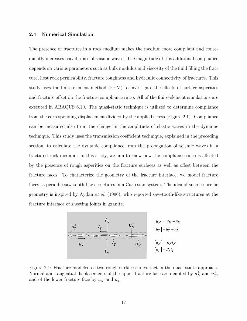
2.4 Numerical Simulation

The presence of fractures in a rock medium makes the medium more compliant and conse-

quently increases travel times of seismic waves. The magnitude of this additional compliance

depends on various parameters such as bulk modulus and viscosity of the fluid filling the frac-

ture, host rock permeability, fracture roughness and hydraulic connectivity of fractures. This

study uses the finite-element method (FEM) to investigate the effects of surface asperities

and fracture offset on the fracture compliance ratio. All of the finite-element simulations are

executed in ABAQUS 6.10. The quasi-static technique is utilized to determine compliance

from the corresponding displacement divided by the applied stress (Figure 2.1). Compliance

can be measured also from the change in the amplitude of elastic waves in the dynamic

technique. This study uses the transmission coefficient technique, explained in the preceding

section, to calculate the dynamic compliance from the propagation of seismic waves in a

fractured rock medium. In this study, we aim to show how the compliance ratio is affected

by the presence of rough asperities on the fracture surfaces as well as offset between the

fracture faces. To characterize the geometry of the fracture interface, we model fracture

faces as periodic saw-tooth-like structures in a Cartesian system. The idea of such a specific

geometry is inspired by Aydan et al. (1996), who reported saw-tooth-like structures at the

fracture interface of sheeting joints in granite.

Figure 2.1: Fracture modeled as two rough surfaces in contact in the quasi-static approach.Normal and tangential displacements of the upper fracture face are denoted by u+

N and u+T ,

and of the lower fracture face by u−N and u−T .

17

Numerical experiments are performed for a single fracture with a rough interface located

in an infinite domain. The two tips of the one-meter-long fracture are in full contact. The

infinite domain has a size of 5000 × 5000 m2 which can be considered as an infinite domain

compare to the size of the fracture as the fracture has a length of 1 m in the horizontal

direction. Infinite elements at the surrounding boundaries are used to eliminate the effect

of reflection from the boundaries. The 2D FEM, illustrated in Figure 2.2, is discretized

adaptively to achieve the desired accuracy. Fracture roughness is modeled as saw-tooth-like

structures with a single spectral component, whose wavelength is much shorter than the total

length of the fracture. Each asperity on each fracture face is meshed with 10 quadrilateral

quadratic elements for the quasi-static analysis; however, it is increased to 100 elements in

the dynamic model per each asperity. As shown in Figure 2.2, saw-tooth-like asperities have

two main angles, that are called Asperity Angle I and Asperity Angle II. These angles are

defined to eliminate any ambiguity in further analysis of the numerical results. The asperity

length shown in Figure 2.2 is assumed to be 1 cm. Therefore, asperity height can be adjusted

by changing the asperity angles.

To improve the numerical accuracy, a refined mesh is used along the rough fracture faces

to capture the high stress concentrations at the sharp corners. Friction between sliding

fracture faces is simulated by the classical isotropic Coulomb friction model that considers a

small sliding with a pre-defined friction coefficient. In the dynamic approach, a seismic plane

wave with angular frequency of 100rad

sand amplitude of 10−12 m is transmitted at a point

0.0001 m above the fracture. The receiver point is located at 0.0001 m beneath the fracture

faces. Properties of the host rock and fracture are presented in Table 2.1. It is assumed that

the matrix has isotropic elastic properties.

To verify the accuracy of our numerical model, the quasi-static compliance ratio of a single

smooth crack in a 2D infinite domain is compared with the analytical solution (Budiansky

and O’Connell, 1976; Kachanov, 1992). The analytical solution suggests a value of 1 for the

compliance ratio. The quasi-static compliance ratio obtained from our numerical model is

18

Figure 2.2: (a) 2D FEM model built to represent a rough fracture. (b) Roughness is modeledwith a right-angled triangle in this specific geometry. Definition of Soft and Stiff directionderives from asymmetry of fracture surface geometry.

Table 2.1: Initial values of rock and fracture parameters.Rock Properties Value UnitYoung’s modulus 60 GPa

Coefficient of sliding friction 0.6Poisson’s ratio 0.25Fracture length 1 mP-wave velocity 5262.35 m.s−1

S-wave velocity 3038.22 m.s−1

1.0007, which is in good agreement with the analytical solution. The dynamic method gives

a compliance ratio of 0.9905 for a single smooth crack located in an infinite medium.

In all of the following figures, the soft compliance ratio and stiff compliance ratio refer

to the quasi-static compliance ratio in the directions shown in Figure 2.2. To calculate the

normal compliance, a tensile stress is applied at the far field and then the excess displace-

19

ment at the center of the fracture is calculated from the difference in the displacement of

corresponding points on the fracture faces. These two corresponding points are at the cen-

ter of the fracture and before applying any stress sharing the same coordinates. The same

procedure is followed for the shear compliance, applying a shear stress at the far field with

the same magnitude as the tensile stress and measuring the excess displacements between

the corresponding points at the center of the fracture. The in-plane direction in this study

is considered as the reference direction as we are only interested to investigate the behavior

of the fracture during its opening. Figures 2.3 to 2.10 give the quasi-static compliance ra-

tios calculated from the stress-displacement measurements. The dynamic compliance ratio

obtained from the attenuation of the transmitted seismic wave is presented in Figures 2.11

and 2.12.

2.5 Results and Discussion

The results of the quasi-static approach can be categorized in two different scenarios. In

the first scenario, there is neither normal nor tangential offset between fracture faces, and

all of the asperities on one fracture face are fully in contact with the corresponding ones on

the other face. This case corresponds to Figures 2.3 to 2.5. The effect of offset and partial

contact is investigated in the second scenario. The offset between fracture faces, in our study,

may be either normal or tangential. The second case corresponds to Figures 2.8 to 2.10.

Interface roughness controls the degree of fracture deformation. However, the area of

contact is not only a function of interface roughness, but also a function of the effective

stress. In our numerical study, the differences between the compliance ratios in the soft

and stiff directions may be explained by the two mechanisms of riding up and interlocking

which describe the interactions of asperities under shearing (Scholzs, 2002). In the riding

up mechanism which is more dominant in the soft direction and for the smaller values of

asperity angle I, a fracture face may ride up on the other face for the applied shear stress in

soft direction. In this case, the effective friction which controls the riding up of two fracture

20

faces is a function of intrinsic friction and the magnitude of asperity angle I. However,

interlocking mechanism is more dominant in the stiff direction and for the larger values of

the asperity angle II. Based on this discussion, interlocking can provide more resistance than

the purely frictional resistance manifesting in the riding up mechanism.

In Figures 2.3 and 2.4, it is assumed that fracture faces are initially perfectly matched so

that there is no offset between fracture faces. Although the asperity angles in these figures

are changing, the area of contact at the fracture faces is roughly constant because the size

of asperities is very small and they are perfectly in contact. As a result, interlocking of

asperities at the fracture faces controls the magnitude of the compliance ratios.

Figure 2.3 shows how compliance ratio varies with a change in asperity angle I if asperity

angle II has a constant value of 90. Asperity angle I is changing from 0 to 15. The

numerical results in Figure 2.3 are compared with the analytical solution of a single smooth

crack, with no interaction at the fracture interface. The analytical solution gives a compliance

ratio of 1 for a smooth crack in 2D. In reality, the assumption of extremely smooth cracks

is not realistic. As discussed earlier, fractures have irregular faces and the presence of these

irregularities control fracture mechanical and hydro-mechanical properties, seismicity and

stress heterogeneity. Figure 2.3 shows how compliance ratio in the presence of saw-tooth-

like structures at the fracture interface deviates from the value of 1 given by the analytical

solution. Smaller values of asperity angle I represent fractures with smoother faces. For

the values of asperity angle I close to zero, there is no difference in the compliance ratio

in different shear directions as there is no preference for sliding in either of the soft or

stiff directions. Therefore, the compliance ratios are independent of the direction of shear

stress, and agree with the analytical solution. This agreement breaks down as asperity angle

I increases, which provides more resistance against sliding. The source of this additional

resistance in the stiff direction is the interlocking of opposing saw-tooth-like structures.

However, the additional resistance in the soft direction may be explained by the larger

frictional resistance and larger compression induced by the larger values of asperity angle

21

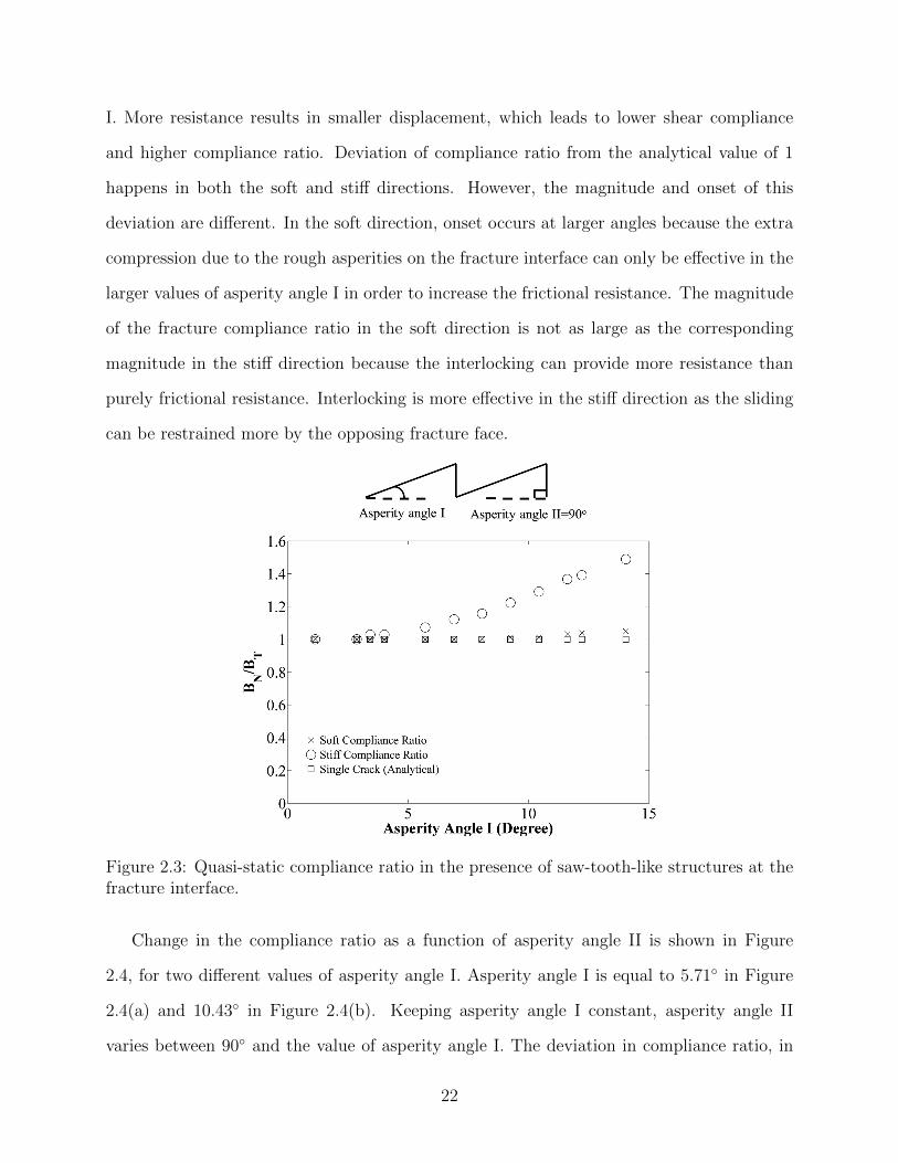
I. More resistance results in smaller displacement, which leads to lower shear compliance

and higher compliance ratio. Deviation of compliance ratio from the analytical value of 1

happens in both the soft and stiff directions. However, the magnitude and onset of this

deviation are different. In the soft direction, onset occurs at larger angles because the extra

compression due to the rough asperities on the fracture interface can only be effective in the

larger values of asperity angle I in order to increase the frictional resistance. The magnitude

of the fracture compliance ratio in the soft direction is not as large as the corresponding

magnitude in the stiff direction because the interlocking can provide more resistance than

purely frictional resistance. Interlocking is more effective in the stiff direction as the sliding

can be restrained more by the opposing fracture face.

Figure 2.3: Quasi-static compliance ratio in the presence of saw-tooth-like structures at thefracture interface.

Change in the compliance ratio as a function of asperity angle II is shown in Figure

2.4, for two different values of asperity angle I. Asperity angle I is equal to 5.71 in Figure

2.4(a) and 10.43 in Figure 2.4(b). Keeping asperity angle I constant, asperity angle II

varies between 90 and the value of asperity angle I. The deviation in compliance ratio, in

22

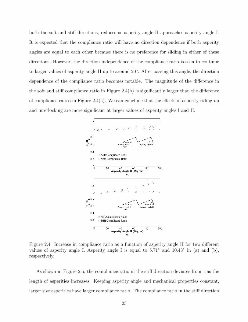
both the soft and stiff directions, reduces as asperity angle II approaches asperity angle I.

It is expected that the compliance ratio will have no direction dependence if both asperity

angles are equal to each other because there is no preference for sliding in either of these

directions. However, the direction independence of the compliance ratio is seen to continue

to larger values of asperity angle II up to around 20. After passing this angle, the direction

dependence of the compliance ratio becomes notable. The magnitude of the difference in

the soft and stiff compliance ratio in Figure 2.4(b) is significantly larger than the difference

of compliance ratios in Figure 2.4(a). We can conclude that the effects of asperity riding up

and interlocking are more significant at larger values of asperity angles I and II.

Figure 2.4: Increase in compliance ratio as a function of asperity angle II for two differentvalues of asperity angle I. Asperity angle I is equal to 5.71 and 10.43 in (a) and (b),respectively.

As shown in Figure 2.5, the compliance ratio in the stiff direction deviates from 1 as the

length of asperities increases. Keeping asperity angle and mechanical properties constant,

larger size asperities have larger compliance ratio. The compliance ratio in the stiff direction

23

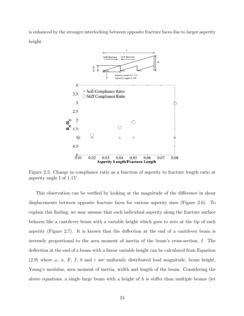
is enhanced by the stronger interlocking between opposite fracture faces due to larger asperity

height.

Figure 2.5: Change in compliance ratio as a function of asperity to fracture length ratio atasperity angle I of 1.15.

This observation can be verified by looking at the magnitude of the difference in shear

displacements between opposite fracture faces for various asperity sizes (Figure 2.6). To

explain this finding, we may assume that each individual asperity along the fracture surface

behaves like a cantilever beam with a variable height which goes to zero at the tip of each

asperity (Figure 2.7). It is known that the deflection at the end of a cantilever beam is

inversely proportional to the area moment of inertia of the beam’s cross-section, I. The

deflection at the end of a beam with a linear variable height can be calculated from Equation

(2.9) where ω, a, E, I, b and c are uniformly distributed load magnitude, beam height,

Young’s modulus, area moment of inertia, width and length of the beam. Considering the

above equations, a single large beam with a height of h is stiffer than multiple beams (let

24

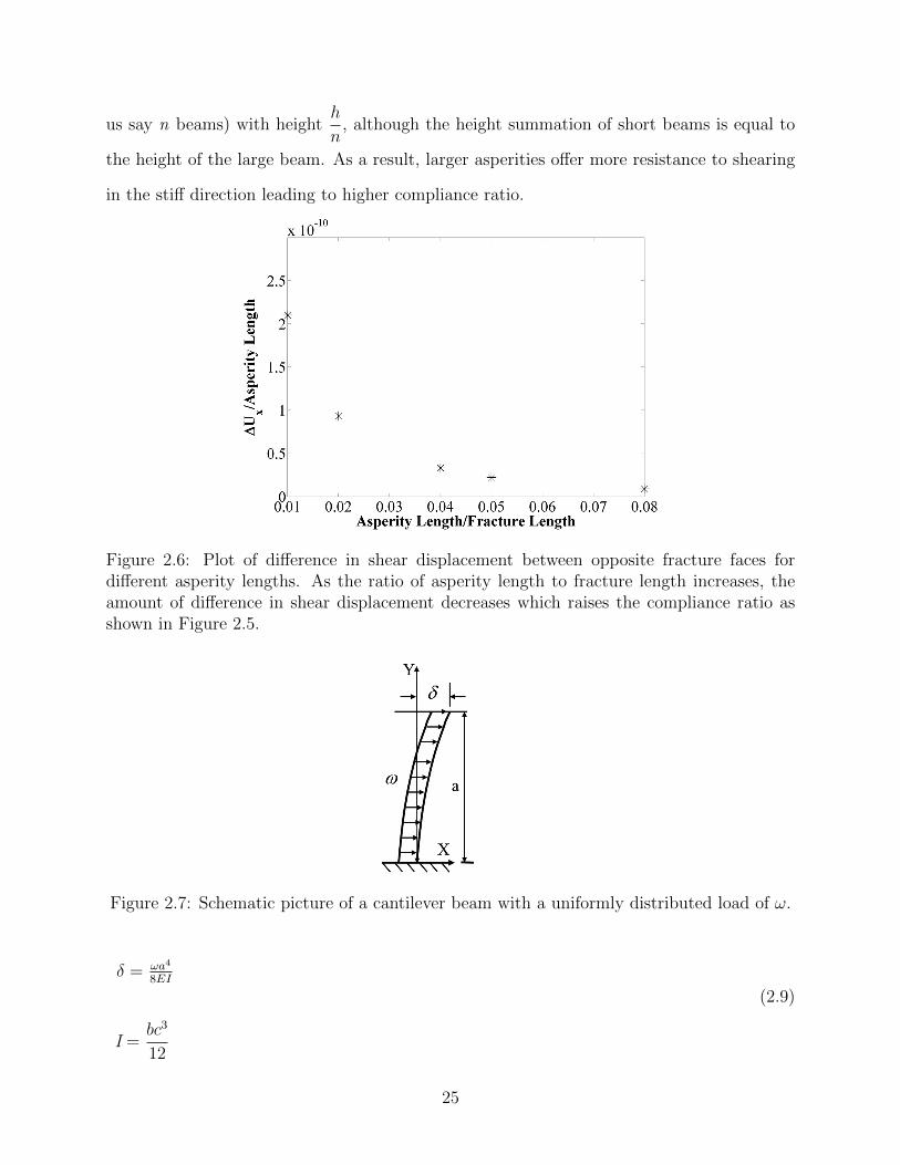
us say n beams) with heighth

n, although the height summation of short beams is equal to

the height of the large beam. As a result, larger asperities offer more resistance to shearing

in the stiff direction leading to higher compliance ratio.

Figure 2.6: Plot of difference in shear displacement between opposite fracture faces fordifferent asperity lengths. As the ratio of asperity length to fracture length increases, theamount of difference in shear displacement decreases which raises the compliance ratio asshown in Figure 2.5.

Figure 2.7: Schematic picture of a cantilever beam with a uniformly distributed load of ω.

δ = ωa4

8EI

I =bc3

12

(2.9)

25

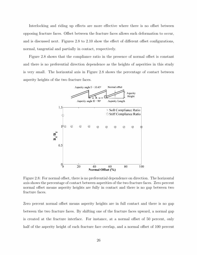
Interlocking and riding up effects are more effective where there is no offset between

opposing fracture faces. Offset between the fracture faces allows such deformation to occur,

and is discussed next. Figures 2.8 to 2.10 show the effect of different offset configurations,

normal, tangential and partially in contact, respectively.

Figure 2.8 shows that the compliance ratio in the presence of normal offset is constant

and there is no preferential direction dependence as the heights of asperities in this study

is very small. The horizontal axis in Figure 2.8 shows the percentage of contact between

asperity heights of the two fracture faces.

Figure 2.8: For normal offset, there is no preferential dependence on direction. The horizontalaxis shows the percentage of contact between asperities of the two fracture faces. Zero percentnormal offset means asperity heights are fully in contact and there is no gap between twofracture faces.

Zero percent normal offset means asperity heights are in full contact and there is no gap

between the two fracture faces. By shifting one of the fracture faces upward, a normal gap

is created at the fracture interface. For instance, at a normal offset of 50 percent, only

half of the asperity height of each fracture face overlap, and a normal offset of 100 percent

26

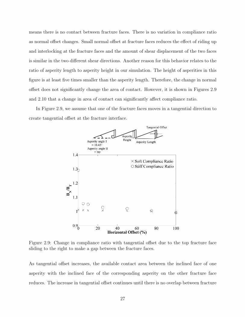
means there is no contact between fracture faces. There is no variation in compliance ratio

as normal offset changes. Small normal offset at fracture faces reduces the effect of riding up

and interlocking at the fracture faces and the amount of shear displacement of the two faces

is similar in the two different shear directions. Another reason for this behavior relates to the

ratio of asperity length to asperity height in our simulation. The height of asperities in this

figure is at least five times smaller than the asperity length. Therefore, the change in normal

offset does not significantly change the area of contact. However, it is shown in Figures 2.9

and 2.10 that a change in area of contact can significantly affect compliance ratio.

In Figure 2.9, we assume that one of the fracture faces moves in a tangential direction to

create tangential offset at the fracture interface.

Figure 2.9: Change in compliance ratio with tangential offset due to the top fracture facesliding to the right to make a gap between the fracture faces.

As tangential offset increases, the available contact area between the inclined face of one

asperity with the inclined face of the corresponding asperity on the other fracture face

reduces. The increase in tangential offset continues until there is no overlap between fracture

27

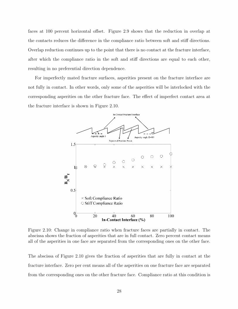
faces at 100 percent horizontal offset. Figure 2.9 shows that the reduction in overlap at

the contacts reduces the difference in the compliance ratio between soft and stiff directions.

Overlap reduction continues up to the point that there is no contact at the fracture interface,

after which the compliance ratio in the soft and stiff directions are equal to each other,

resulting in no preferential direction dependence.

For imperfectly mated fracture surfaces, asperities present on the fracture interface are

not fully in contact. In other words, only some of the asperities will be interlocked with the

corresponding asperities on the other fracture face. The effect of imperfect contact area at

the fracture interface is shown in Figure 2.10.

Figure 2.10: Change in compliance ratio when fracture faces are partially in contact. Theabscissa shows the fraction of asperities that are in full contact. Zero percent contact meansall of the asperities in one face are separated from the corresponding ones on the other face.

The abscissa of Figure 2.10 gives the fraction of asperities that are fully in contact at the

fracture interface. Zero per cent means all of the asperities on one fracture face are separated

from the corresponding ones on the other fracture face. Compliance ratio at this condition is

28

equal to the compliance ratio of dry or gas-filled fractures. With an increase in the percentage

of contact between the fracture faces, the deviation in compliance ratio between soft and

stiff direction increases. The largest difference happens when all of the asperities are fully

in contact. Figure 2.10 demonstrates that the compliance ratio is a function of the number

of in-contact faces along the fracture interface. An increase in the number of in-contact

faces magnifies the compliance ratio discrepancy by increasing the effects of riding up and

interlocking.

The numerical results of Figures 2.3 to 2.10 can be compared with the analytical solution

for a fracture with in-contact faces of Yoshioka and Scholz (1989a) and Yoshioka and Scholz

(1989b). Yoshioka and Scholz derived analytical solutions for normal and shear compliance

of imperfectly bonded fracture faces. They used the distribution of local Hertzian spheres to

mimic in-contact fracture faces. They assumed a no-slip condition in their solution. In their

model, fracture faces are under compressive stress, leading to closure of the fracture. These

sphere-made fracture faces provides smoother fracture interfaces compare to the saw-tooth

structures considered in this study and observed in the field. Based on their assumptions,

Yoshioka and Scholz concluded that the compliance ratio in imperfectly bonded interfaces

only depends on Poisson’s ratio, shown in Equation (2.10). This equation does not predict the

direction dependence of the compliance ratio for imperfectly bonded fracture faces subject

to a tensile stress and underestimates the compliance ratio. This formula shows that the

compliance ratio equals 0.3043 for a Poisson’s ratio of 0.25, which is significantly smaller

than the ratios obtained in this study.

BN

BT

= 0.711− ν2− ν

(2.10)

Fracture compliance can be derived from either the quasi-static or dynamic technique.

As mentioned above, stress−displacement measurements determine compliance in the quasi-

static technique. Fracture compliance can be also derived from the change in properties of

29

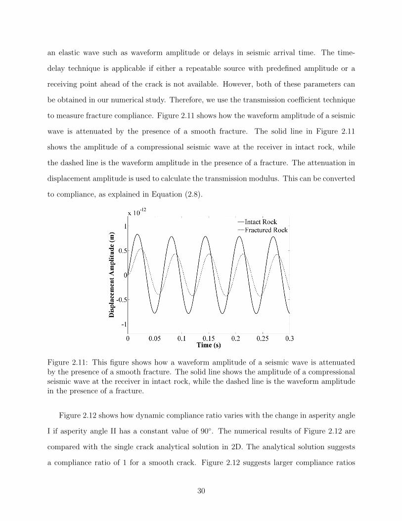
an elastic wave such as waveform amplitude or delays in seismic arrival time. The time-

delay technique is applicable if either a repeatable source with predefined amplitude or a

receiving point ahead of the crack is not available. However, both of these parameters can

be obtained in our numerical study. Therefore, we use the transmission coefficient technique

to measure fracture compliance. Figure 2.11 shows how the waveform amplitude of a seismic

wave is attenuated by the presence of a smooth fracture. The solid line in Figure 2.11

shows the amplitude of a compressional seismic wave at the receiver in intact rock, while

the dashed line is the waveform amplitude in the presence of a fracture. The attenuation in

displacement amplitude is used to calculate the transmission modulus. This can be converted

to compliance, as explained in Equation (2.8).

Figure 2.11: This figure shows how a waveform amplitude of a seismic wave is attenuatedby the presence of a smooth fracture. The solid line shows the amplitude of a compressionalseismic wave at the receiver in intact rock, while the dashed line is the waveform amplitudein the presence of a fracture.

Figure 2.12 shows how dynamic compliance ratio varies with the change in asperity angle

I if asperity angle II has a constant value of 90. The numerical results of Figure 2.12 are

compared with the single crack analytical solution in 2D. The analytical solution suggests

a compliance ratio of 1 for a smooth crack. Figure 2.12 suggests larger compliance ratios

30

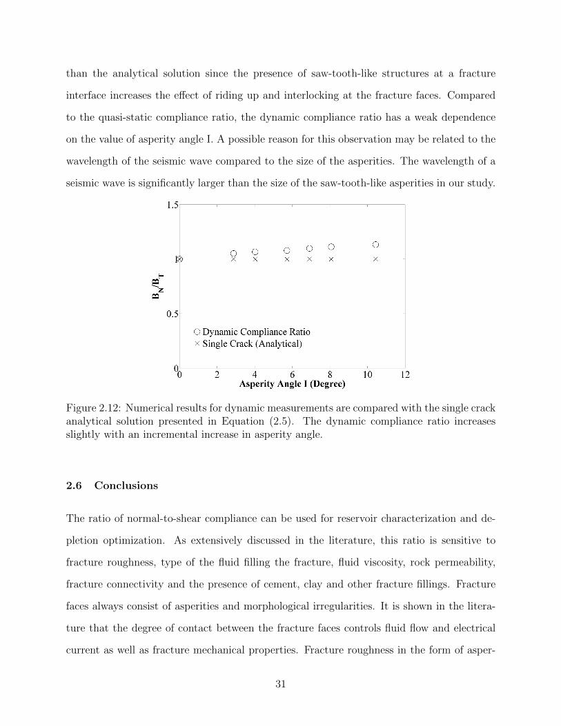
than the analytical solution since the presence of saw-tooth-like structures at a fracture

interface increases the effect of riding up and interlocking at the fracture faces. Compared

to the quasi-static compliance ratio, the dynamic compliance ratio has a weak dependence

on the value of asperity angle I. A possible reason for this observation may be related to the

wavelength of the seismic wave compared to the size of the asperities. The wavelength of a

seismic wave is significantly larger than the size of the saw-tooth-like asperities in our study.

Figure 2.12: Numerical results for dynamic measurements are compared with the single crackanalytical solution presented in Equation (2.5). The dynamic compliance ratio increasesslightly with an incremental increase in asperity angle.

2.6 Conclusions

The ratio of normal-to-shear compliance can be used for reservoir characterization and de-

pletion optimization. As extensively discussed in the literature, this ratio is sensitive to

fracture roughness, type of the fluid filling the fracture, fluid viscosity, rock permeability,

fracture connectivity and the presence of cement, clay and other fracture fillings. Fracture

faces always consist of asperities and morphological irregularities. It is shown in the litera-

ture that the degree of contact between the fracture faces controls fluid flow and electrical

current as well as fracture mechanical properties. Fracture roughness in the form of asper-

31

ities might be generated during joint formation or faulting. These features on the surface

of fractures can affect measured compliance ratios. In this study, we employ quasi-static

and dynamic approaches to investigate the effects of contact area and interface offset on the

fracture compliance ratio. We study different geometrical and offset configurations to show

how compliance ratio is a function of available contact area at the fracture interface and

also the size of the asperities. For a single smooth crack in a tensile stress in a 2D infinite

medium, the compliance ratio equals to 1. However, our study shows that compliance ratio

increases to values more than 1 if the fracture has rough faces. The interlocking of asperities

on fracture faces can significantly influence the compliance ratio in the stiff direction. The

deviation in the compliance ratio for the soft direction from 1, suggested by the analytical

solution for a single smooth crack, can be explained by the riding up effect. It is notable

that interlocking is not the only parameter governing the interaction between rough fracture

faces. The contact area between the fracture faces is also controlled by effective stress that

affects the excess of compliance ratio, as shown in Figures 2.8 to 2.10.

2.7 References

Ahmadi, M., A. Dahi Taleghani, and C. M. Sayers. “Direction dependence of fracture com-pliance induced by slickensides.” Geophysics 79, no. 4 (2014): C91-C96.

Aydan, O., Y. Shimizu, and T. Kawamoto. “The anisotropy of surface morphology and shearstrength characteristics of rock discontinuities and its evaluation.” NARMS 96 (1996):1391-1398.

Bachrach, R. “Recent advances in the characterization of unconventional reservoirs withwide-azimuth seismic data.” Unconventional Resources Technology Conference (URTEC),(2013).

Barton, N. “Rock quality, seismic velocity, attenuation and anisotropy.” CRC press, (2007).

Bedayat, H., and A. Dahi Taleghani. “Anisotropic Inhomogeneous Poroelastic Inclusions:With Application to Underground Energy-Related Problems.” Journal of Energy Re-sources Technology 138, no. 3 (2016): 032905.

Boadu, F. K., and L. T. Long. “Effects of fractures on seismic-wave velocity and attenuation.”Geophysical Journal International 127, no. 1 (1996): 86-110.

32

Brown, S. R. “Transport of fluid and electric current through a single fracture.” Journal ofGeophysical Research: Solid Earth 94, no. B7 (1989): 9429-9438.

Budiansky, B., and R. J. O’Connell. “Elastic moduli of a cracked solid.” International Journalof Solids and Structures 12, no. 2 (1976): 81-97.

Candela, Th., F. Renard, M. Bouchon, A. Brouste, D. Marsan, J. Schmittbuhl, and Ch.Voisin. “Characterization of fault roughness at various scales: Implications of three-dimensional high resolution topography measurements.” Pure and Applied Geophysics166, no. 10-11 (2009): 1817-1851.

Durney, D. W, and J. G. Ramsay. “Incremental strains measured by syntectonic crystalgrowths.” Gravity and tectonics 67 (1973): 96.

Gale, J. FW, R. M. Reed, and J. Holder. “Natural fractures in the Barnett Shale and theirimportance for hydraulic fracture treatments.” AAPG bulletin 91, no. 4 (2007): 603-622.

Hobday, C., and M. H. Worthington. “Field measurements of normal and shear fracturecompliance.” Geophysical Prospecting 60, no. 3 (2012): 488-499.

Hudson, J. A., E. Liu, and S. Crampin. “The mechanical properties of materials with inter-connected cracks and pores.” Geophysical Journal International 124, no. 1 (1996): 105-112.

Kachanov, M. “Effective elastic properties of cracked solids: critical review of some basicconcepts.” Applied Mechanics Reviews 45, no. 8 (1992): 304-335.

Laubach, S., R. Marrett, and J. Olson. “New directions in fracture characterization.” TheLeading Edge 19, no. 7 (2000): 704-711.

Leucci, G., and L. De Giorgi. “Experimental studies on the effects of fracture on the P andS wave velocity propagation in sedimentary rock.” Engineering Geology 84, no. 3 (2006):130-142.

Liu, E. “Effects of fracture aperture and roughness on hydraulic and mechanical proper-ties of rocks: implication of seismic characterization of fractured reservoirs.” Journal ofGeophysics and Engineering 2, no. 1 (2005): 38.

Liu, E., J. H. Queen, X. Y. Li, M. Chapman, S. Maultzsch, H. B. Lynn, and E. M. Chesnokov.“Observation and analysis of frequency-dependent anisotropy from a multicomponent VSPat Bluebell-Altamont field, Utah.” Journal of Applied Geophysics 54, no. 3 (2003): 319-333.

Lubbe, R., J. Sothcott, M. H. Worthington, and C. McCann. “Laboratory estimates ofnormal and shear fracture compliance.” Geophysical Prospecting 56, no. 2 (2008): 239-247.

MacBeth, C., and H. Schuett. “The stress dependent elastic properties of thermally inducedmicrofractures in aeolian Rotliegend sandstone.” Geophysical Prospecting 55, no. 3 (2007):323-332.

33

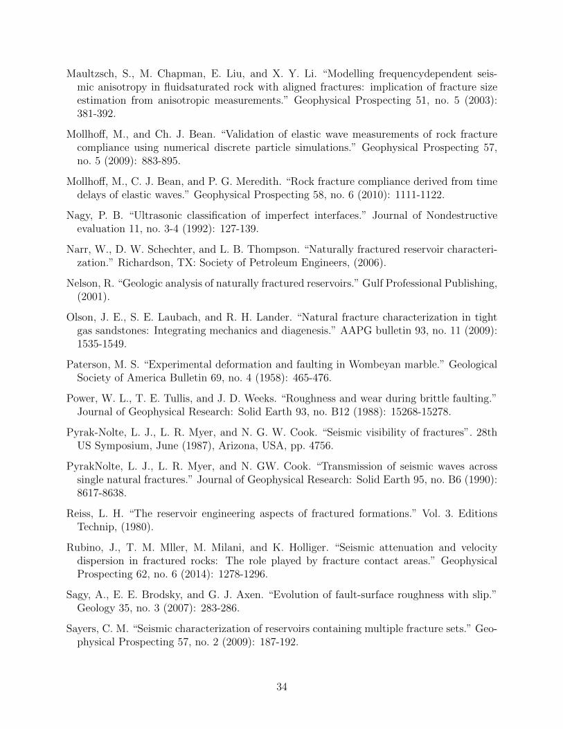
Maultzsch, S., M. Chapman, E. Liu, and X. Y. Li. “Modelling frequencydependent seis-mic anisotropy in fluidsaturated rock with aligned fractures: implication of fracture sizeestimation from anisotropic measurements.” Geophysical Prospecting 51, no. 5 (2003):381-392.

Mollhoff, M., and Ch. J. Bean. “Validation of elastic wave measurements of rock fracturecompliance using numerical discrete particle simulations.” Geophysical Prospecting 57,no. 5 (2009): 883-895.

Mollhoff, M., C. J. Bean, and P. G. Meredith. “Rock fracture compliance derived from timedelays of elastic waves.” Geophysical Prospecting 58, no. 6 (2010): 1111-1122.

Nagy, P. B. “Ultrasonic classification of imperfect interfaces.” Journal of Nondestructiveevaluation 11, no. 3-4 (1992): 127-139.

Narr, W., D. W. Schechter, and L. B. Thompson. “Naturally fractured reservoir characteri-zation.” Richardson, TX: Society of Petroleum Engineers, (2006).

Nelson, R. “Geologic analysis of naturally fractured reservoirs.” Gulf Professional Publishing,(2001).

Olson, J. E., S. E. Laubach, and R. H. Lander. “Natural fracture characterization in tightgas sandstones: Integrating mechanics and diagenesis.” AAPG bulletin 93, no. 11 (2009):1535-1549.

Paterson, M. S. “Experimental deformation and faulting in Wombeyan marble.” GeologicalSociety of America Bulletin 69, no. 4 (1958): 465-476.

Power, W. L., T. E. Tullis, and J. D. Weeks. “Roughness and wear during brittle faulting.”Journal of Geophysical Research: Solid Earth 93, no. B12 (1988): 15268-15278.

Pyrak-Nolte, L. J., L. R. Myer, and N. G. W. Cook. “Seismic visibility of fractures”. 28thUS Symposium, June (1987), Arizona, USA, pp. 4756.

PyrakNolte, L. J., L. R. Myer, and N. GW. Cook. “Transmission of seismic waves acrosssingle natural fractures.” Journal of Geophysical Research: Solid Earth 95, no. B6 (1990):8617-8638.

Reiss, L. H. “The reservoir engineering aspects of fractured formations.” Vol. 3. EditionsTechnip, (1980).

Rubino, J., T. M. Mller, M. Milani, and K. Holliger. “Seismic attenuation and velocitydispersion in fractured rocks: The role played by fracture contact areas.” GeophysicalProspecting 62, no. 6 (2014): 1278-1296.

Sagy, A., E. E. Brodsky, and G. J. Axen. “Evolution of fault-surface roughness with slip.”Geology 35, no. 3 (2007): 283-286.

Sayers, C. M. “Seismic characterization of reservoirs containing multiple fracture sets.” Geo-physical Prospecting 57, no. 2 (2009): 187-192.

34

Sayers, C. M., and M. Kachanov. “A simple technique for finding effective elastic constantsof cracked solids for arbitrary crack orientation statistics.” International Journal of Solidsand Structures 27, no. 6 (1991): 671-680.

Sayers, C. M., and M. Kachanov. “Microcrackinduced elastic wave anisotropy of brittlerocks.” Journal of Geophysical Research: Solid Earth 100, no. B3 (1995): 4149-4156.

Sayers, C. M., A. Dahi Taleghani, and J. Adachi. “The effect of mineralization on the ratio ofnormal to tangential compliance of fractures.” Geophysical Prospecting 57, no. 3 (2009):439-446.

Schoenberg, M. “Elastic wave behavior across linear slip interfaces.” The Journal of theAcoustical Society of America 68, no. 5 (1980): 1516-1521.

Schoenberg, M., and C. M. Sayers. “Seismic anisotropy of fractured rock.” Geophysics 60,no. 1 (1995): 204-211.

Scholz, Ch. H. “The mechanics of earthquakes and faulting.” Cambridge university press,(2002).

Verdon, J. P., and A. Wustefeld. “Measurement of the normal/tangential fracture compli-ance ratio (ZN/ZT) during hydraulic fracture stimulation using Swave splitting data.”Geophysical Prospecting 61, no. s1 (2013): 461-475.

Van Dam, D. B., and C. J. de Pater. “Roughness of hydraulic fractures: The importanceof in-situ stress and tip processes.” In SPE Annual Technical Conference and Exhibition.Society of Petroleum Engineers, (1999).

Yoshioka, N., and Ch. H. Scholz. “Elastic properties of contacting surfaces under normal andshear loads, 1, Theory.” Journal of Geophysics. Res 94, no. B12 (1989): 17681-17690.

Yoshioka, N., and Ch. H. Scholz. “Elastic properties of contacting surfaces under normal andshear loads: 2. Comparison of theory with experiment.” Journal of Geophysical Research:Solid Earth 94, no. B12 (1989): 17691-17700.

35

Chapter 3Impact of Thermally Reactivated Micro-Natural Fractures on Well Productiv-ity in Shale Reservoirs

3.1 Introduction

Hydraulic fracturing treatments have played a crucial role in boosting hydrocarbon pro-

duction from low permeability reservoirs. Induced fractures significantly improve wellbore-

formation contact area and consequently increase the production rate. Injection of highly

pressurized fracturing fluid fractures the formation to create a highly permeable conduit for

the reservoir fluid to produce. The direction of hydraulic fracture propagation depends on

the direction of the minimum principal stress as well as natural fractures (Economides and

Nolte, 2000; Dahi Taleghani and Olson, 2011). Core and outcrop studies, advanced logging

tools, microseismic techniques and well testing analysis have proved the existence of natural

fractures in many unconventional reservoirs. In naturally fractured reservoirs, arrest and

diversion of hydraulic fracture front into the pre-existing natural fractures have been the

subject of many experimental and theoretical studies (Warpinski and Teufel, 2010; Potluri

et al., 2005; Dahi Taleghani et al., 2013; Gonzalez et al., 2015).

Natural fractures are mechanical discontinuities with the lengths varying from microm-

eters to kilometers (Narr et al., 2006). These fractures may act as conductive paths for

the fluid flow in the low permeability reservoirs affecting the ultimate recovery. However,

they can also increase the leakoff volume during the fracturing treatments leading to early

36

screenouts or poorly propped hydraulic fractures. Contribution of natural fractures in the

hydrocarbon recovery is more significant in the tight formations with low permeability than

permeable reservoirs (Nelson, 2001). Existence of natural fractures in the outcrop samples

could be an indicative of their existence in the subsurface; however, characterization of nat-

ural fractures in subsurface is not a trivial task. Most of the outcrop studies are qualitative

and the existing models studying the interaction of natural fractures with the hydraulic

fracture mainly consider the contribution of large natural fractures, i.e. fractures with the

dimensions comparable to the size of hydraulic fracture, on the hydraulic fracture growth

(Jeffrey et al., 2009; Dahi Taleghani and Olson, 2014). However, the log-normal distribution

of natural fractures, shown in Figure 3.1, demonstrates that small natural fracture exist

orders of magnitudes more frequent than the large natural fractures. Hence, the role of

small-size natural fractures may be as important as the large natural fractures since the

small fractures exist in large numbers. Length of small natural fractures varies from micro-

to centi- meter; therefore, injected proppants cannot enter inside these small fractures to

keep them open.

Figure 3.1: Power-law aperture-size distribution in Groove Creek and Kinlaw formationsshows much larger frequency of micro-fractures in comparison to large size fractures (Plotborrowed from Gale, 2002).

37

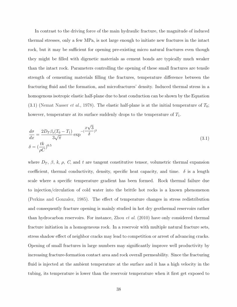
In contrast to the driving force of the main hydraulic fracture, the magnitude of induced

thermal stresses, only a few MPa, is not large enough to initiate new fractures in the intact

rock, but it may be sufficient for opening pre-existing micro natural fractures even though

they might be filled with digenetic materials as cement bonds are typically much weaker

than the intact rock. Parameters controlling the opening of these small fractures are tensile

strength of cementing materials filling the fractures, temperature difference between the

fracturing fluid and the formation, and microfractures’ density. Induced thermal stress in a

homogenous isotropic elastic half-plane due to heat conduction can be shown by the Equation

(3.1) (Nemat Nasser et al., 1978). The elastic half-plane is at the initial temperature of T0;

however, temperature at its surface suddenly drops to the temperature of T1.

dσ

dx=

2DTβs(T0 − T1)

3√π

exp−(x√

3

δ)2

δ = (tk

ρC)0.5

(3.1)

where DT , β, k, ρ, C, and t are tangent constitutive tensor, volumetric thermal expansion

coefficient, thermal conductivity, density, specific heat capacity, and time. δ is a length

scale where a specific temperature gradient has been formed. Rock thermal failure due

to injection/circulation of cold water into the brittle hot rocks is a known phenomenon

(Perkins and Gonzalez, 1985). The effect of temperature changes in stress redistribution

and consequently fracture opening is mainly studied in hot dry geothermal reservoirs rather

than hydrocarbon reservoirs. For instance, Zhou et al. (2010) have only considered thermal

fracture initiation in a homogeneous rock. In a reservoir with multiple natural fracture sets,

stress shadow effect of neighbor cracks may lead to competition or arrest of advancing cracks.

Opening of small fractures in large numbers may significantly improve well productivity by

increasing fracture-formation contact area and rock overall permeability. Since the fracturing

fluid is injected at the ambient temperature at the surface and it has a high velocity in the

tubing, its temperature is lower than the reservoir temperature when it first get exposed to

38

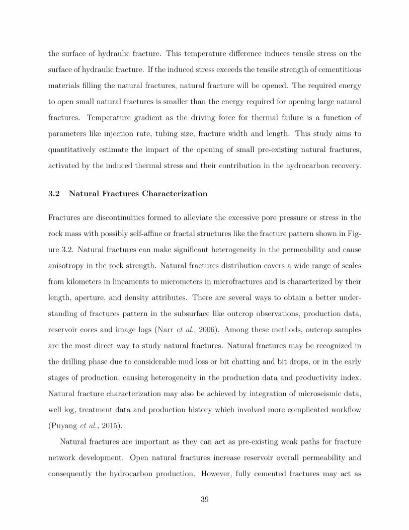
the surface of hydraulic fracture. This temperature difference induces tensile stress on the

surface of hydraulic fracture. If the induced stress exceeds the tensile strength of cementitious

materials filling the natural fractures, natural fracture will be opened. The required energy

to open small natural fractures is smaller than the energy required for opening large natural

fractures. Temperature gradient as the driving force for thermal failure is a function of

parameters like injection rate, tubing size, fracture width and length. This study aims to

quantitatively estimate the impact of the opening of small pre-existing natural fractures,

activated by the induced thermal stress and their contribution in the hydrocarbon recovery.

3.2 Natural Fractures Characterization

Fractures are discontinuities formed to alleviate the excessive pore pressure or stress in the

rock mass with possibly self-affine or fractal structures like the fracture pattern shown in Fig-

ure 3.2. Natural fractures can make significant heterogeneity in the permeability and cause

anisotropy in the rock strength. Natural fractures distribution covers a wide range of scales

from kilometers in lineaments to micrometers in microfractures and is characterized by their

length, aperture, and density attributes. There are several ways to obtain a better under-

standing of fractures pattern in the subsurface like outcrop observations, production data,

reservoir cores and image logs (Narr et al., 2006). Among these methods, outcrop samples

are the most direct way to study natural fractures. Natural fractures may be recognized in

the drilling phase due to considerable mud loss or bit chatting and bit drops, or in the early

stages of production, causing heterogeneity in the production data and productivity index.

Natural fracture characterization may also be achieved by integration of microseismic data,

well log, treatment data and production history which involved more complicated workflow

(Puyang et al., 2015).

Natural fractures are important as they can act as pre-existing weak paths for fracture

network development. Open natural fractures increase reservoir overall permeability and

consequently the hydrocarbon production. However, fully cemented fractures may act as

39

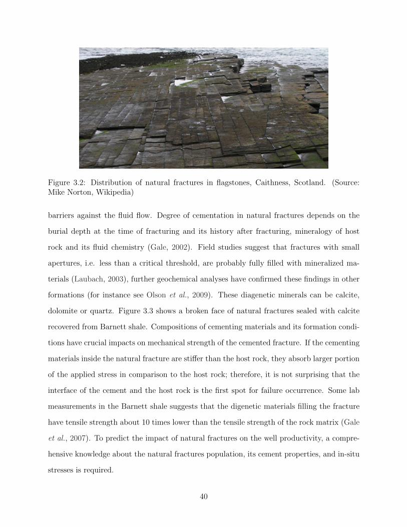
Figure 3.2: Distribution of natural fractures in flagstones, Caithness, Scotland. (Source:Mike Norton, Wikipedia)

barriers against the fluid flow. Degree of cementation in natural fractures depends on the

burial depth at the time of fracturing and its history after fracturing, mineralogy of host

rock and its fluid chemistry (Gale, 2002). Field studies suggest that fractures with small

apertures, i.e. less than a critical threshold, are probably fully filled with mineralized ma-

terials (Laubach, 2003), further geochemical analyses have confirmed these findings in other

formations (for instance see Olson et al., 2009). These diagenetic minerals can be calcite,

dolomite or quartz. Figure 3.3 shows a broken face of natural fractures sealed with calcite

recovered from Barnett shale. Compositions of cementing materials and its formation condi-

tions have crucial impacts on mechanical strength of the cemented fracture. If the cementing

materials inside the natural fracture are stiffer than the host rock, they absorb larger portion

of the applied stress in comparison to the host rock; therefore, it is not surprising that the

interface of the cement and the host rock is the first spot for failure occurrence. Some lab

measurements in the Barnett shale suggests that the digenetic materials filling the fracture

have tensile strength about 10 times lower than the tensile strength of the rock matrix (Gale

et al., 2007). To predict the impact of natural fractures on the well productivity, a compre-

hensive knowledge about the natural fractures population, its cement properties, and in-situ

stresses is required.

40

Figure 3.3: Broken surface of natural fractures sealed with calcite in Barnett Shale. (Bor-rowed from Gale et al., 2007)

3.3 Natural Fractures Characterization

Linear elastic fracture mechanics (LEFM) is powerful tool to model fracture behavior in

brittle rocks, however, it fails to predict fracture propagation in soft rocks. Lack of capability

to predict fracture initiation is another drawback of LEFM. Cohesive zone method (CZM) is

a substitute theory for LEFM to study fracture behaviors without the described limitations.

Cohesive zone model can predict fracture initiation and propagation in brittle, ductile, and

cemented materials. Dugdale (1960) and Barenblatt (1962) introduced the theory of cohesive

zones to incorporate material inelastic behavior at the fracture tips. In the cohesive zone

model, Barenblatt assumed that molecular cohesive forces create a non-linear bonding zone

at the crack tip while tensile strength and cohesive toughness control the damage of these

bonds. This technique removes the stress singularity at fracture tips by introducing cohesive

forces to address one of the main drawbacks of LEFM.

Elices et al. (2002) discussed the advantages and limitations of the CZM in a review

paper. A significant limitation in CZM is the pre-defined path for fracture propagation which

requires that the pre-defined path supporting rock failure should be known or dynamically

41

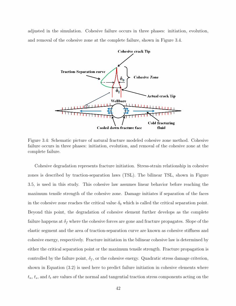
adjusted in the simulation. Cohesive failure occurs in three phases: initiation, evolution,

and removal of the cohesive zone at the complete failure, shown in Figure 3.4.

Figure 3.4: Schematic picture of natural fracture modeled cohesive zone method. Cohesivefailure occurs in three phases: initiation, evolution, and removal of the cohesive zone at thecomplete failure.

Cohesive degradation represents fracture initiation. Stress-strain relationship in cohesive

zones is described by traction-separation laws (TSL). The bilinear TSL, shown in Figure

3.5, is used in this study. This cohesive law assumes linear behavior before reaching the

maximum tensile strength of the cohesive zone. Damage initiates if separation of the faces

in the cohesive zone reaches the critical value δ0 which is called the critical separation point.

Beyond this point, the degradation of cohesive element further develops as the complete

failure happens at δf where the cohesive forces are gone and fracture propagates. Slope of the

elastic segment and the area of traction-separation curve are known as cohesive stiffness and

cohesive energy, respectively. Fracture initiation in the bilinear cohesive law is determined by

either the critical separation point or the maximum tensile strength. Fracture propagation is

controlled by the failure point, δf , or the cohesive energy. Quadratic stress damage criterion,

shown in Equation (3.2) is used here to predict failure initiation in cohesive elements where

tn, ts, and tt are values of the normal and tangential traction stress components acting on the

42

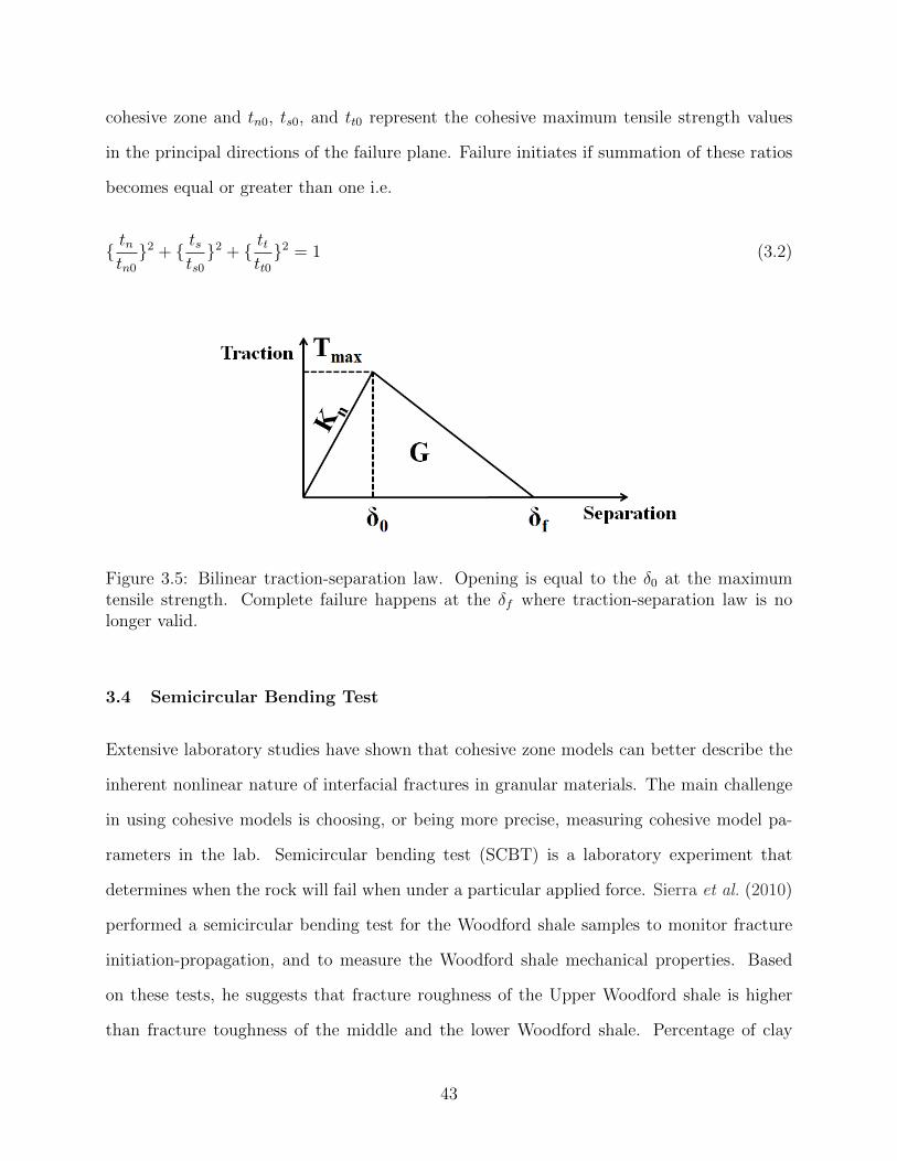
cohesive zone and tn0, ts0, and tt0 represent the cohesive maximum tensile strength values

in the principal directions of the failure plane. Failure initiates if summation of these ratios

becomes equal or greater than one i.e.

tntn0

2 + tsts02 + tt

tt02 = 1 (3.2)

Figure 3.5: Bilinear traction-separation law. Opening is equal to the δ0 at the maximumtensile strength. Complete failure happens at the δf where traction-separation law is nolonger valid.

3.4 Semicircular Bending Test

Extensive laboratory studies have shown that cohesive zone models can better describe the

inherent nonlinear nature of interfacial fractures in granular materials. The main challenge

in using cohesive models is choosing, or being more precise, measuring cohesive model pa-

rameters in the lab. Semicircular bending test (SCBT) is a laboratory experiment that

determines when the rock will fail when under a particular applied force. Sierra et al. (2010)

performed a semicircular bending test for the Woodford shale samples to monitor fracture

initiation-propagation, and to measure the Woodford shale mechanical properties. Based

on these tests, he suggests that fracture roughness of the Upper Woodford shale is higher

than fracture toughness of the middle and the lower Woodford shale. Percentage of clay

43

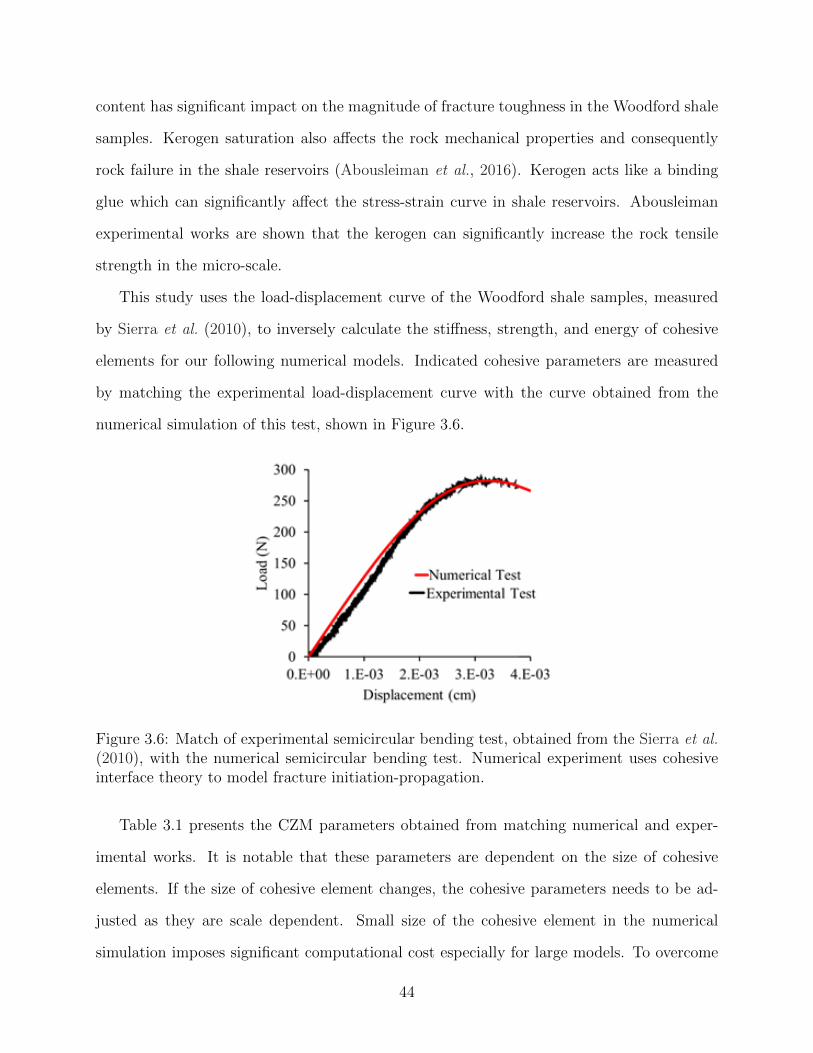
content has significant impact on the magnitude of fracture toughness in the Woodford shale

samples. Kerogen saturation also affects the rock mechanical properties and consequently

rock failure in the shale reservoirs (Abousleiman et al., 2016). Kerogen acts like a binding

glue which can significantly affect the stress-strain curve in shale reservoirs. Abousleiman

experimental works are shown that the kerogen can significantly increase the rock tensile

strength in the micro-scale.

This study uses the load-displacement curve of the Woodford shale samples, measured

by Sierra et al. (2010), to inversely calculate the stiffness, strength, and energy of cohesive

elements for our following numerical models. Indicated cohesive parameters are measured

by matching the experimental load-displacement curve with the curve obtained from the

numerical simulation of this test, shown in Figure 3.6.

Figure 3.6: Match of experimental semicircular bending test, obtained from the Sierra et al.(2010), with the numerical semicircular bending test. Numerical experiment uses cohesiveinterface theory to model fracture initiation-propagation.

Table 3.1 presents the CZM parameters obtained from matching numerical and exper-

imental works. It is notable that these parameters are dependent on the size of cohesive

elements. If the size of cohesive element changes, the cohesive parameters needs to be ad-

justed as they are scale dependent. Small size of the cohesive element in the numerical

simulation imposes significant computational cost especially for large models. To overcome

44

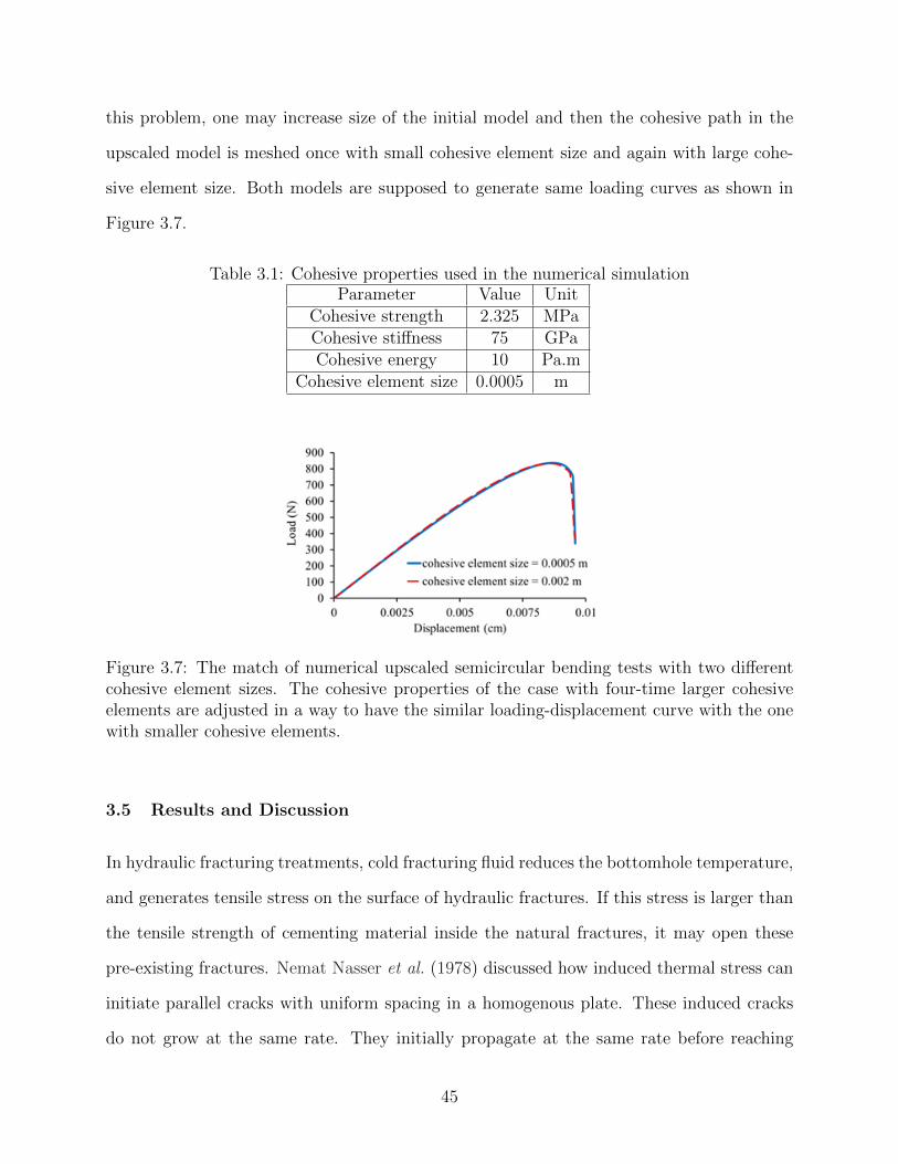
this problem, one may increase size of the initial model and then the cohesive path in the

upscaled model is meshed once with small cohesive element size and again with large cohe-

sive element size. Both models are supposed to generate same loading curves as shown in

Figure 3.7.

Table 3.1: Cohesive properties used in the numerical simulationParameter Value Unit

Cohesive strength 2.325 MPaCohesive stiffness 75 GPaCohesive energy 10 Pa.m

Cohesive element size 0.0005 m

Figure 3.7: The match of numerical upscaled semicircular bending tests with two differentcohesive element sizes. The cohesive properties of the case with four-time larger cohesiveelements are adjusted in a way to have the similar loading-displacement curve with the onewith smaller cohesive elements.

3.5 Results and Discussion

In hydraulic fracturing treatments, cold fracturing fluid reduces the bottomhole temperature,

and generates tensile stress on the surface of hydraulic fractures. If this stress is larger than

the tensile strength of cementing material inside the natural fractures, it may open these

pre-existing fractures. Nemat Nasser et al. (1978) discussed how induced thermal stress can

initiate parallel cracks with uniform spacing in a homogenous plate. These induced cracks

do not grow at the same rate. They initially propagate at the same rate before reaching

45

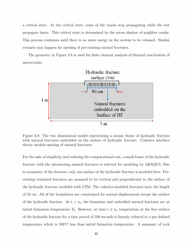
a critical state. At the critical state, some of the cracks stop propagating while the rest

propagate faster. This critical state is determined by the stress shadow of neighbor cracks.

This process continues until there is no more energy in the system to be released. Similar

scenario may happen for opening of pre-existing natural fractures.

The geometry in Figure 3.8 is used for finite element analysis of thermal reactivation of

microcracks.

Figure 3.8: The two dimensional model representing a mosaic frame of hydraulic fracturewith natural fractures embedded on the surface of hydraulic fracture. Cohesive interfacetheory models opening of natural fractures.

For the sake of simplicity and reducing the computational cost, a small frame of the hydraulic

fracture with the intersecting natural fractures is selected for modeling by ABAQUS. Due

to symmetry of the fracture, only one surface of the hydraulic fracture is modeled here. Pre-

existing cemented fractures are assumed to be vertical and perpendicular to the surface of

the hydraulic fracture modeled with CZM. The cohesive-modeled fractures have the length

of 10 cm. All of the boundaries are constrained for normal displacement except the surface

of the hydraulic fracture. At t < t0, the formation and embedded natural fractures are at

initial formation temperature T0. However, at time t > t0, temperature at the free surface

of the hydraulic fracture for a time period of 100 seconds is linearly reduced to a pre-defined

temperature which is 100C less than initial formation temperature. A summary of rock

46

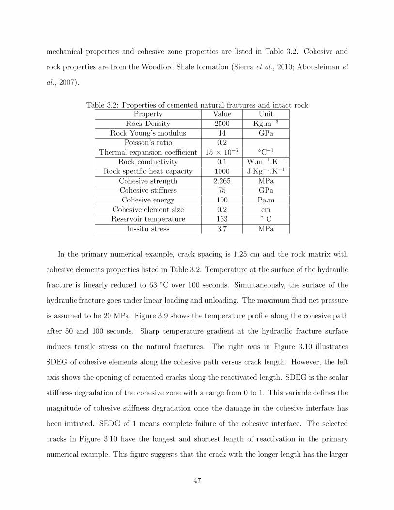
mechanical properties and cohesive zone properties are listed in Table 3.2. Cohesive and

rock properties are from the Woodford Shale formation (Sierra et al., 2010; Abousleiman et

al., 2007).

Table 3.2: Properties of cemented natural fractures and intact rockProperty Value Unit

Rock Density 2500 Kg.m−3

Rock Young’s modulus 14 GPaPoisson’s ratio 0.2

Thermal expansion coefficient 15 × 10−6 C−1

Rock conductivity 0.1 W.m−1.K−1

Rock specific heat capacity 1000 J.Kg−1.K−1

Cohesive strength 2.265 MPaCohesive stiffness 75 GPaCohesive energy 100 Pa.m

Cohesive element size 0.2 cmReservoir temperature 163 C

In-situ stress 3.7 MPa

In the primary numerical example, crack spacing is 1.25 cm and the rock matrix with

cohesive elements properties listed in Table 3.2. Temperature at the surface of the hydraulic

fracture is linearly reduced to 63 C over 100 seconds. Simultaneously, the surface of the

hydraulic fracture goes under linear loading and unloading. The maximum fluid net pressure

is assumed to be 20 MPa. Figure 3.9 shows the temperature profile along the cohesive path

after 50 and 100 seconds. Sharp temperature gradient at the hydraulic fracture surface

induces tensile stress on the natural fractures. The right axis in Figure 3.10 illustrates

SDEG of cohesive elements along the cohesive path versus crack length. However, the left

axis shows the opening of cemented cracks along the reactivated length. SDEG is the scalar

stiffness degradation of the cohesive zone with a range from 0 to 1. This variable defines the

magnitude of cohesive stiffness degradation once the damage in the cohesive interface has

been initiated. SEDG of 1 means complete failure of the cohesive interface. The selected

cracks in Figure 3.10 have the longest and shortest length of reactivation in the primary

numerical example. This figure suggests that the crack with the longer length has the larger

47

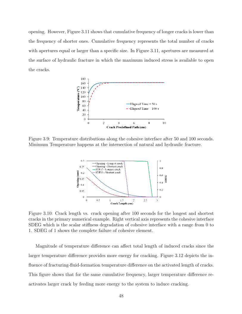
opening. However, Figure 3.11 shows that cumulative frequency of longer cracks is lower than

the frequency of shorter ones. Cumulative frequency represents the total number of cracks

with apertures equal or larger than a specific size. In Figure 3.11, apertures are measured at

the surface of hydraulic fracture in which the maximum induced stress is available to open

the cracks.

Figure 3.9: Temperature distributions along the cohesive interface after 50 and 100 seconds.Minimum Temperature happens at the intersection of natural and hydraulic fracture.

Figure 3.10: Crack length vs. crack opening after 100 seconds for the longest and shortestcracks in the primary numerical example. Right vertical axis represents the cohesive interfaceSDEG which is the scalar stiffness degradation of cohesive interface with a range from 0 to1. SDEG of 1 shows the complete failure of cohesive element.

Magnitude of temperature difference can affect total length of induced cracks since the

larger temperature difference provides more energy for cracking. Figure 3.12 depicts the in-

fluence of fracturing-fluid-formation temperature difference on the activated length of cracks.

This figure shows that for the same cumulative frequency, larger temperature difference re-

activates larger crack by feeding more energy to the system to induce cracking.

48

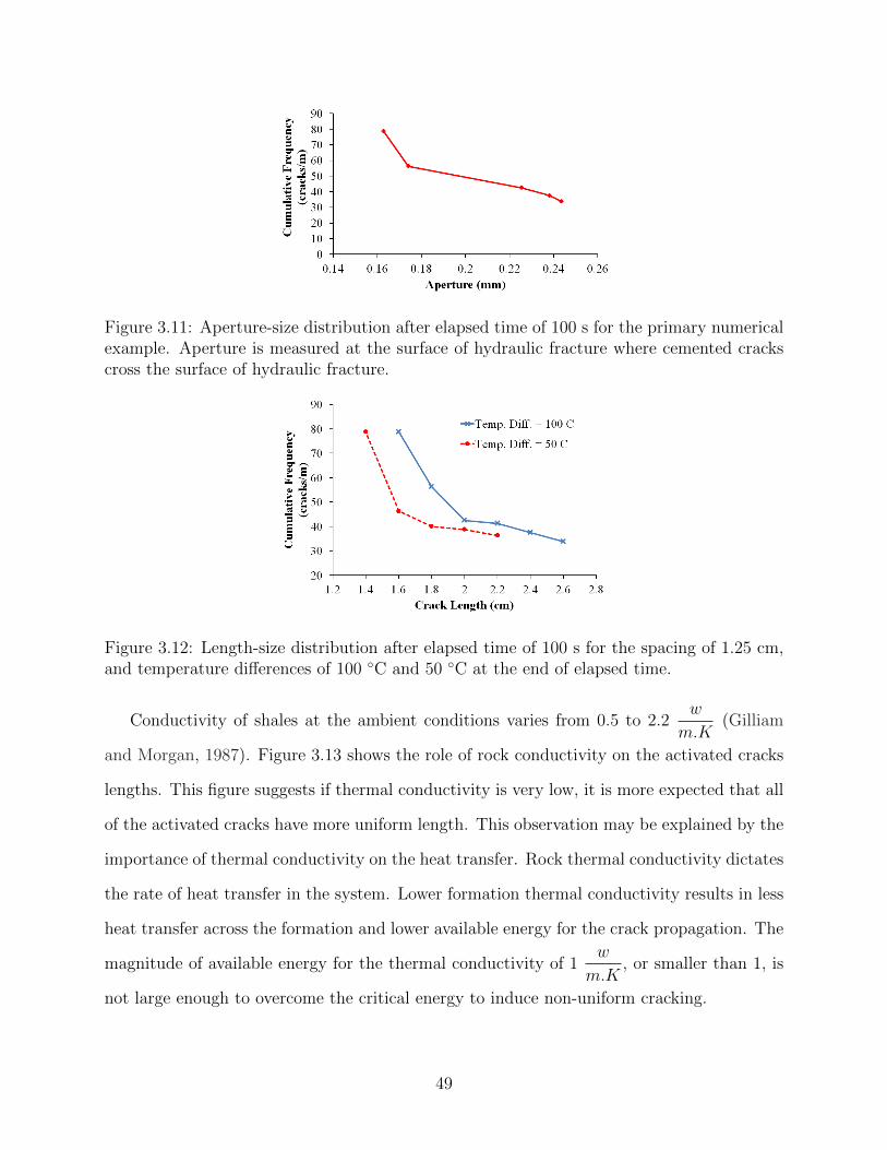
Figure 3.11: Aperture-size distribution after elapsed time of 100 s for the primary numericalexample. Aperture is measured at the surface of hydraulic fracture where cemented crackscross the surface of hydraulic fracture.

Figure 3.12: Length-size distribution after elapsed time of 100 s for the spacing of 1.25 cm,and temperature differences of 100 C and 50 C at the end of elapsed time.

Conductivity of shales at the ambient conditions varies from 0.5 to 2.2w

m.K(Gilliam

and Morgan, 1987). Figure 3.13 shows the role of rock conductivity on the activated cracks

lengths. This figure suggests if thermal conductivity is very low, it is more expected that all

of the activated cracks have more uniform length. This observation may be explained by the

importance of thermal conductivity on the heat transfer. Rock thermal conductivity dictates

the rate of heat transfer in the system. Lower formation thermal conductivity results in less

heat transfer across the formation and lower available energy for the crack propagation. The

magnitude of available energy for the thermal conductivity of 1w

m.K, or smaller than 1, is

not large enough to overcome the critical energy to induce non-uniform cracking.

49

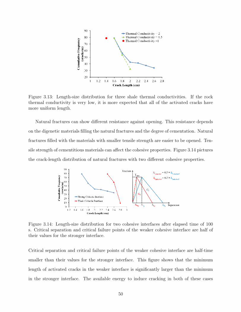
Figure 3.13: Length-size distribution for three shale thermal conductivities. If the rockthermal conductivity is very low, it is more expected that all of the activated cracks havemore uniform length.

Natural fractures can show different resistance against opening. This resistance depends

on the digenetic materials filling the natural fractures and the degree of cementation. Natural

fractures filled with the materials with smaller tensile strength are easier to be opened. Ten-

sile strength of cementitious materials can affect the cohesive properties. Figure 3.14 pictures

the crack-length distribution of natural fractures with two different cohesive properties.

Figure 3.14: Length-size distribution for two cohesive interfaces after elapsed time of 100s. Critical separation and critical failure points of the weaker cohesive interface are half oftheir values for the stronger interface.

Critical separation and critical failure points of the weaker cohesive interface are half-time

smaller than their values for the stronger interface. This figure shows that the minimum

length of activated cracks in the weaker interface is significantly larger than the minimum

in the stronger interface. The available energy to induce cracking in both of these cases

50

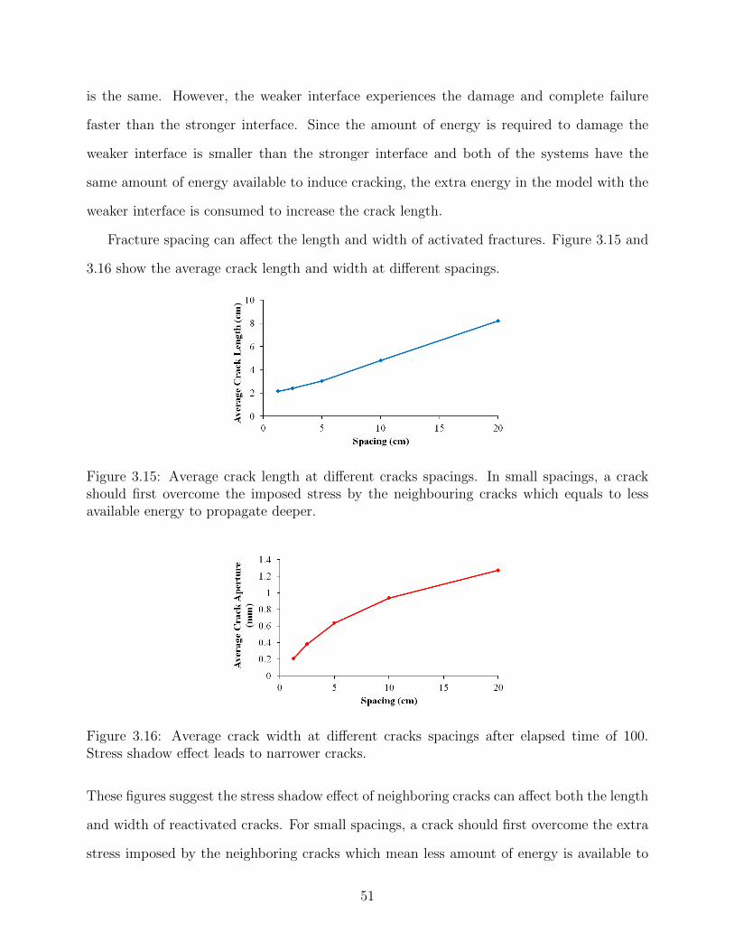
is the same. However, the weaker interface experiences the damage and complete failure

faster than the stronger interface. Since the amount of energy is required to damage the

weaker interface is smaller than the stronger interface and both of the systems have the

same amount of energy available to induce cracking, the extra energy in the model with the

weaker interface is consumed to increase the crack length.

Fracture spacing can affect the length and width of activated fractures. Figure 3.15 and

3.16 show the average crack length and width at different spacings.

Figure 3.15: Average crack length at different cracks spacings. In small spacings, a crackshould first overcome the imposed stress by the neighbouring cracks which equals to lessavailable energy to propagate deeper.

Figure 3.16: Average crack width at different cracks spacings after elapsed time of 100.Stress shadow effect leads to narrower cracks.

These figures suggest the stress shadow effect of neighboring cracks can affect both the length

and width of reactivated cracks. For small spacings, a crack should first overcome the extra

stress imposed by the neighboring cracks which mean less amount of energy is available to

51

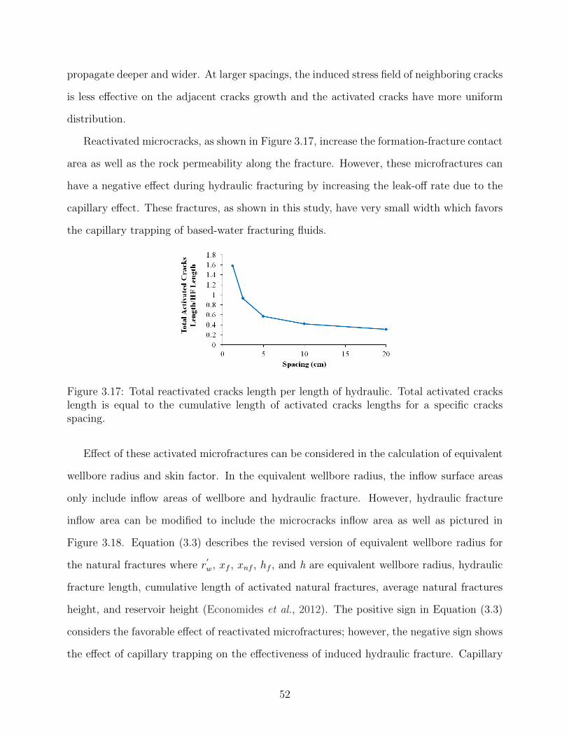
propagate deeper and wider. At larger spacings, the induced stress field of neighboring cracks

is less effective on the adjacent cracks growth and the activated cracks have more uniform

distribution.

Reactivated microcracks, as shown in Figure 3.17, increase the formation-fracture contact

area as well as the rock permeability along the fracture. However, these microfractures can

have a negative effect during hydraulic fracturing by increasing the leak-off rate due to the

capillary effect. These fractures, as shown in this study, have very small width which favors

the capillary trapping of based-water fracturing fluids.

Figure 3.17: Total reactivated cracks length per length of hydraulic. Total activated crackslength is equal to the cumulative length of activated cracks lengths for a specific cracksspacing.

Effect of these activated microfractures can be considered in the calculation of equivalent

wellbore radius and skin factor. In the equivalent wellbore radius, the inflow surface areas

only include inflow areas of wellbore and hydraulic fracture. However, hydraulic fracture

inflow area can be modified to include the microcracks inflow area as well as pictured in

Figure 3.18. Equation (3.3) describes the revised version of equivalent wellbore radius for

the natural fractures where r′w, xf , xnf , hf , and h are equivalent wellbore radius, hydraulic

fracture length, cumulative length of activated natural fractures, average natural fractures

height, and reservoir height (Economides et al., 2012). The positive sign in Equation (3.3)

considers the favorable effect of reactivated microfractures; however, the negative sign shows

the effect of capillary trapping on the effectiveness of induced hydraulic fracture. Capillary

52

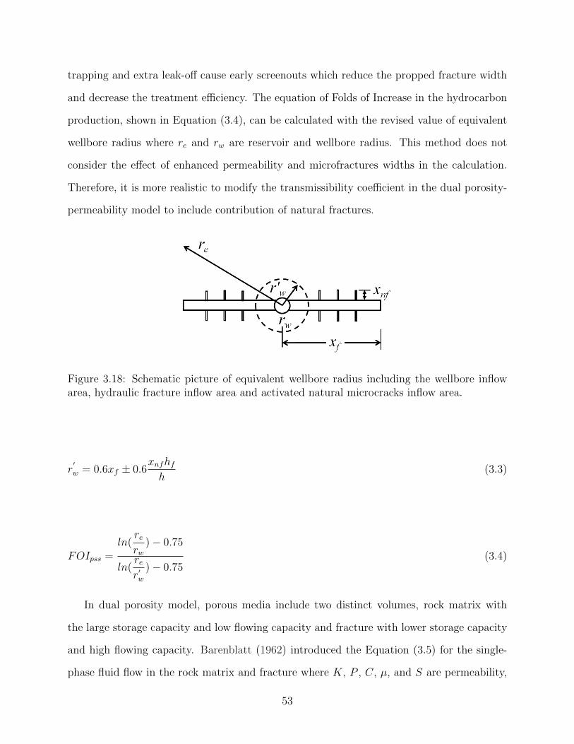
trapping and extra leak-off cause early screenouts which reduce the propped fracture width

and decrease the treatment efficiency. The equation of Folds of Increase in the hydrocarbon

production, shown in Equation (3.4), can be calculated with the revised value of equivalent

wellbore radius where re and rw are reservoir and wellbore radius. This method does not

consider the effect of enhanced permeability and microfractures widths in the calculation.

Therefore, it is more realistic to modify the transmissibility coefficient in the dual porosity-

permeability model to include contribution of natural fractures.

Figure 3.18: Schematic picture of equivalent wellbore radius including the wellbore inflowarea, hydraulic fracture inflow area and activated natural microcracks inflow area.

r′

w = 0.6xf ± 0.6xnfhfh

(3.3)

FOIpss =ln(

rerw

)− 0.75

ln(rer′w

)− 0.75(3.4)

In dual porosity model, porous media include two distinct volumes, rock matrix with

the large storage capacity and low flowing capacity and fracture with lower storage capacity

and high flowing capacity. Barenblatt (1962) introduced the Equation (3.5) for the single-

phase fluid flow in the rock matrix and fracture where K, P , C, µ, and S are permeability,

53

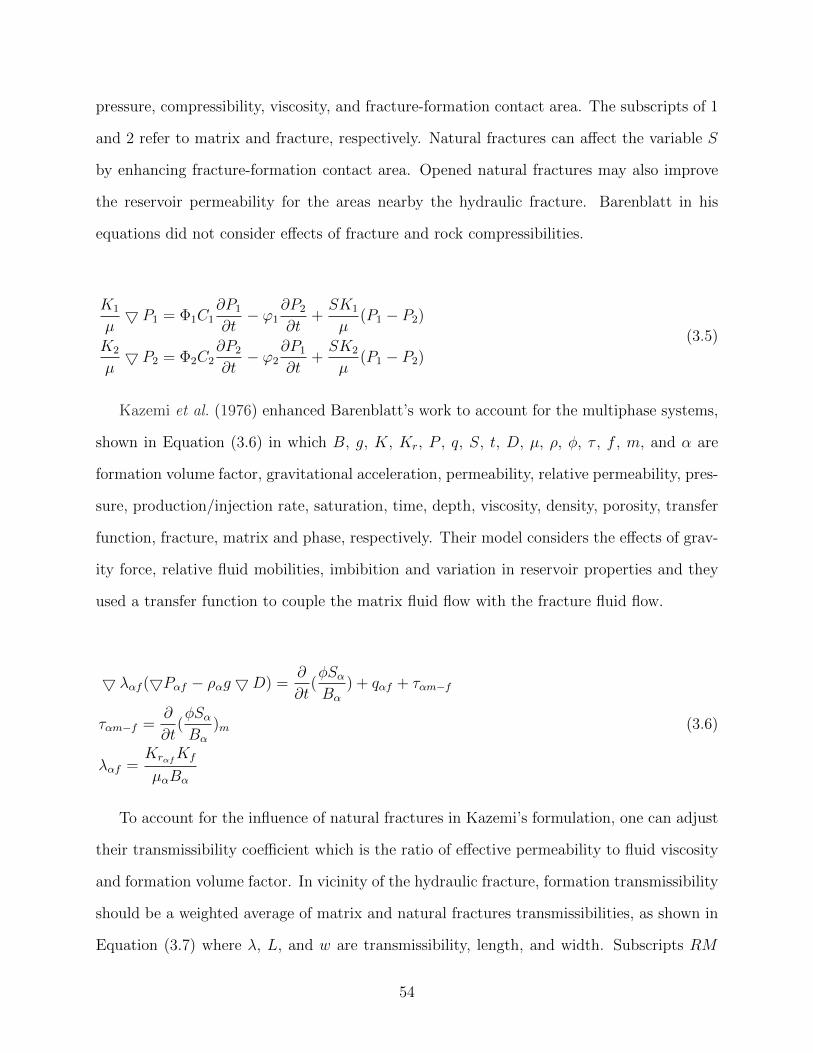
pressure, compressibility, viscosity, and fracture-formation contact area. The subscripts of 1

and 2 refer to matrix and fracture, respectively. Natural fractures can affect the variable S

by enhancing fracture-formation contact area. Opened natural fractures may also improve

the reservoir permeability for the areas nearby the hydraulic fracture. Barenblatt in his

equations did not consider effects of fracture and rock compressibilities.

K1

µ5 P1 = Φ1C1

∂P1

∂t− ϕ1

∂P2

∂t+SK1

µ(P1 − P2)

K2

µ5 P2 = Φ2C2

∂P2

∂t− ϕ2

∂P1

∂t+SK2

µ(P1 − P2)

(3.5)

Kazemi et al. (1976) enhanced Barenblatt’s work to account for the multiphase systems,

shown in Equation (3.6) in which B, g, K, Kr, P , q, S, t, D, µ, ρ, φ, τ , f , m, and α are

formation volume factor, gravitational acceleration, permeability, relative permeability, pres-

sure, production/injection rate, saturation, time, depth, viscosity, density, porosity, transfer

function, fracture, matrix and phase, respectively. Their model considers the effects of grav-

ity force, relative fluid mobilities, imbibition and variation in reservoir properties and they

used a transfer function to couple the matrix fluid flow with the fracture fluid flow.

5 λαf (5Pαf − ραg5D) =∂

∂t(φSαBα

) + qαf + ταm−f

ταm−f =∂

∂t(φSαBα

)m

λαf =KrαfKf

µαBα

(3.6)

To account for the influence of natural fractures in Kazemi’s formulation, one can adjust

their transmissibility coefficient which is the ratio of effective permeability to fluid viscosity

and formation volume factor. In vicinity of the hydraulic fracture, formation transmissibility

should be a weighted average of matrix and natural fractures transmissibilities, as shown in

Equation (3.7) where λ, L, and w are transmissibility, length, and width. Subscripts RM

54

and NF refer to rock matrix and natural fracture. Figure 3.19 illustrates the schematic

picture of a reservoir block including rock matrix and reactivated natural fractures. This

modified transmissibility coefficient, considering the effect of natural fractures, can be used

for areas in the vicinity of hydraulic fracture.

Figure 3.19: Schematic picture of a reservoir block including rock matrix and reactivatednatural fractures.

KNF =w2NF

12

λ =LNF + LRMLNF∑N

1 wNFnλNF + wRMλRM∑N1 wNFn + wRM

+LRMλRM

(3.7)

In the low permeable shale reservoirs, hydrocarbon production from the hydraulic frac-

tures and natural fractures dictates the economic success of a well. To illustrate effect

of micro-natural fractures in hydrocarbon production, the cumulative gas production in a

hydraulically fractured shale reservoir, having a horizontal well, can be compared for two

different scenarios where the reactivated cracks either do or do not cross the surface of hy-

draulic fracture. In this reservoir simulation, effect of capillary trapping is ignored for the

sake of simplicity, and it is assumed that all of the reactivated natural fractures boost fluid

flow from the reservoir into the wellbore. As it is shown in Figure 3.10, crack opening reduces

with crack length. To determine cracks length and width in the reservoir simulation, it is

55

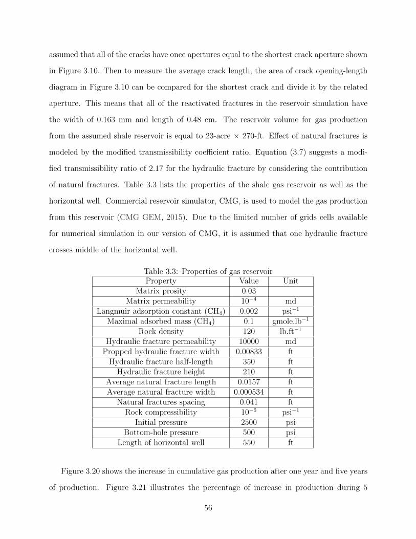
assumed that all of the cracks have once apertures equal to the shortest crack aperture shown

in Figure 3.10. Then to measure the average crack length, the area of crack opening-length

diagram in Figure 3.10 can be compared for the shortest crack and divide it by the related

aperture. This means that all of the reactivated fractures in the reservoir simulation have

the width of 0.163 mm and length of 0.48 cm. The reservoir volume for gas production

from the assumed shale reservoir is equal to 23-acre × 270-ft. Effect of natural fractures is

modeled by the modified transmissibility coefficient ratio. Equation (3.7) suggests a modi-

fied transmissibility ratio of 2.17 for the hydraulic fracture by considering the contribution

of natural fractures. Table 3.3 lists the properties of the shale gas reservoir as well as the

horizontal well. Commercial reservoir simulator, CMG, is used to model the gas production

from this reservoir (CMG GEM, 2015). Due to the limited number of grids cells available

for numerical simulation in our version of CMG, it is assumed that one hydraulic fracture

crosses middle of the horizontal well.

Table 3.3: Properties of gas reservoirProperty Value Unit

Matrix prosity 0.03Matrix permeability 10−4 md

Langmuir adsorption constant (CH4) 0.002 psi−1

Maximal adsorbed mass (CH4) 0.1 gmole.lb−1

Rock density 120 lb.ft−1

Hydraulic fracture permeability 10000 mdPropped hydraulic fracture width 0.00833 ft

Hydraulic fracture half-length 350 ftHydraulic fracture height 210 ft

Average natural fracture length 0.0157 ftAverage natural fracture width 0.000534 ft

Natural fractures spacing 0.041 ftRock compressibility 10−6 psi−1

Initial pressure 2500 psiBottom-hole pressure 500 psi

Length of horizontal well 550 ft

Figure 3.20 shows the increase in cumulative gas production after one year and five years

of production. Figure 3.21 illustrates the percentage of increase in production during 5

56

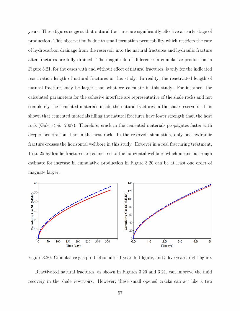
years. These figures suggest that natural fractures are significantly effective at early stage of

production. This observation is due to small formation permeability which restricts the rate

of hydrocarbon drainage from the reservoir into the natural fractures and hydraulic fracture

after fractures are fully drained. The magnitude of difference in cumulative production in

Figure 3.21, for the cases with and without effect of natural fractures, is only for the indicated

reactivation length of natural fractures in this study. In reality, the reactivated length of

natural fractures may be larger than what we calculate in this study. For instance, the

calculated parameters for the cohesive interface are representative of the shale rocks and not

completely the cemented materials inside the natural fractures in the shale reservoirs. It is

shown that cemented materials filling the natural fractures have lower strength than the host

rock (Gale et al., 2007). Therefore, crack in the cemented materials propagates faster with

deeper penetration than in the host rock. In the reservoir simulation, only one hydraulic

fracture crosses the horizontal wellbore in this study. However in a real fracturing treatment,

15 to 25 hydraulic fractures are connected to the horizontal wellbore which means our rough

estimate for increase in cumulative production in Figure 3.20 can be at least one order of

magnate larger.

Figure 3.20: Cumulative gas production after 1 year, left figure, and 5 five years, right figure.

Reactivated natural fractures, as shown in Figures 3.20 and 3.21, can improve the fluid

recovery in the shale reservoirs. However, these small opened cracks can act like a two

57

Figure 3.21: Percentage of increase in cumulative gas production during 5 years in a semi-loggraph.

edged swords. Some of the hydraulic fracturing treatments use water as the based fluid for

fracturing fluid. In water wet formations, since the width of reactivated cracks, as shown

in Figures 3.10 and 3.16, are significantly small, capillary pressure for these cracks can be

large enough to suck in the fracturing fluid and trap it inside the natural fractures. The

reservoir pressure at the early stages of production can push out the trapped water inside

the reactivated natural fractures; however, during production as the water cut increases

along with drop in the reservoir pressure below the capillary pressure, a significant drop in

the hydrocarbon production is expected as the produced water will be trapped inside the

reactivated natural fractures.

3.6 Conclusion

Considerable temperature difference between fracturing fluid and reservoir would induce

thermal tensile stress on the surface of the hydraulic fracture. The induced tensile stresses

may open cemented natural fractures, improving the formation-fracture contact area as well

as enhancing the rock permeability in the vicinity of the hydraulic fracture. Most of natural

fractures are much smaller than the hydraulic fracture; however, their presence in large pop-

ulation can have a considerable impact on production. Right after stimulation, these natural

58

fractures are drained by the drive of reservoir pressure. As production continues and water

cut increases, the water is being trapped in these natural fractures (capillary trapping) and

act as barrier against gas production. Cohesive interface theory has been utilized here to

model reactivation of natural fractures due to induced thermal stresses. Semicircular bend-

ing test of the Woodford shale samples are used to derive cohesive properties required for

numerical simulations. This study suggests that the length and width of reactivated length

depends on the spacing of natural fractures, rock thermal conductivity, temperature differ-

ence between fracturing fluid and reservoir, as well as the strength of diagenetic materials

filling natural fractures. Larger natural fracture spacing results in longer and more uniform

activated cracks since the stress shadow effect diminishes as fracture spacing increases. In-

jecting a colder fracturing fluid into a reservoir with larger thermal conductivity increases

the length of reactivated fractures. The impact of reactivated natural fractures can be trans-

lated into transmissibility coefficient of the hydraulic fracture to incorporate their impact on

permeability enhancement near fractures.

3.7 References

Abousleiman, Y. N., M. H. Tran, S. Hoang, C. P. Bobko, A. Ortega, and F.J. Ulm. “Geome-chanics field and laboratory characterization of the Woodford Shale: The next gas play.”In SPE Annual Technical Conference and Exhibition. Society of Petroleum Engineers,2007.

Abousleiman, Y. N., K. L. Hull, Y. Han, G. Al-Muntasheri, P. Hosemann, S. Parker, andC. B. Howard. “The granular and polymer composite nature of kerogen-rich shale.” ActaGeotechnica: 1-22, 2016.

Barenblatt, G. I. “The mathematical theory of equilibrium cracks in brittle fracture.” Ad-vances in applied mechanics 7.1 (1962): 55-129.

User’s Manual for CMG GEM. Computer Modeling Group Ltd, CMG GEM. 2015: Calgary,Alberta, Canada.

Dahi Taleghani, A., and J. Olson. “Numerical modeling of multistranded-hydraulic-fracturepropagation: accounting for the interaction between induced and natural fractures.” SPEJournal 16.3 (2011): 575-581.

59

Dahi Taleghani, A., M. Ahmadi, and J. E. Olson. “Secondary Fractures and Their PotentialImpacts on Hydraulic Fractures Efficiency.” In ISRM International Conference for Effectiveand Sustainable Hydraulic Fracturing. International Society for Rock Mechanics, 2013.

Dahi Taleghani, A., and J. E. Olson. “How natural fractures could affect hydraulic-fracturegeometry.” SPE Journal 19, no. 01 (2014): 161-171.

Dugdale, D. S. “Yielding of steel sheets containing slits.” Journal of the Mechanics andPhysics of Solids 8.2 (1960): 100-104.

Elices, M., G. V. Guinea, J. Gomez, and J. Planas. “The cohesive zone model: advantages,limitations and challenges.” Engineering fracture mechanics 69, no. 2 (2002): 137-163.

Economides, M. J. and K.G. Nolte. “Reservoir stimulation.” Wiley Press, 2000.

Economides, M. J., A. D. Hill, C. Ehlig-Economides, and D. Zhu. “Petroleum productionsystems.” Pearson Education, 2012.

Gale, J. FW. “Specifying lengths of horizontal wells in fractured reservoirs.” SPE ReservoirEvaluation & Engineering 5.03 (2002): 266-272.

Gale, J. FW, R. M. Reed, and J. Holder. “Natural fractures in the Barnett Shale and theirimportance for hydraulic fracture treatments.” AAPG bulletin 91.4 (2007): 603-622.

Gilliam, T. M., and I. L. Morgan. “Shale: Measurement of thermal properties.” No.ORNL/TM-10499. Oak Ridge National Lab., TN (USA), 1987.

Gonzalez-Chavez, M., P. Puyang, and A. Dahi Taleghani. “From semi-circular bending testto microseismic maps: an integrated modeling approach to incorporate natural fractureeffects on hydraulic fracturing.” Unconventional resources technology conference, SPE.Aug. 2015.

Jeffrey, R., X. Zhang, and M. Thiercelin. “Hydraulic Fracture Offsetting in Naturally Frac-tures Reservoirs: Quantifying a Long-Recognized Process.” SPE Hydraulic FracturingTechnology Conference. 2009.

Kazemi, H., L. S. Merrill Jr, K. L. Porterfield, and P. R. Zeman. ”Numerical simulation ofwater-oil flow in naturally fractured reservoirs.” Society of Petroleum Engineers Journal16, no. 06 (1976): 317-326.

Kresse, O., X. Weng, H. Gu, and R. Wu. “Numerical modeling of hydraulic fractures inter-action in complex naturally fractured formations.” Rock mechanics and rock engineering46, no. 3 (2013): 555-568.

Laubach, S. E. “Practical approaches to identifying sealed and open fractures.” AAPG bul-letin 87.4 (2003): 561-579.

Narr, W., D. S. Schechter, and L. B. Thompson. “Naturally fractured reservoir characteri-zation.” Society of Petroleum Engineers, 2006.

60

Nelson, R. “Geologic analysis of naturally fractured reservoirs.” Gulf Professional Publishing,2001.

Nemat-Nasser, S., L. M. Keer, and K. S. Parihar. “Unstable growth of thermally inducedinteracting cracks in brittle solids.” International Journal of Solids and Structures 14.6(1978): 409-430.

Olson, J. E., S. E. Laubach, and R. H. Lander. “Natural fracture characterization in tight gassandstones: Integrating mechanics and diagenesis.” AAPG bulletin 93.11 (2009): 1535-1549.

Perkins, T. K., and J. A. Gonzalez. “The effect of thermoelastic stresses on injection wellfracturing.” Old SPE Journal 25.1 (1985): 78-88.

Potluri, N. K., D. Zhu, and A. D. Hill. “The effect of natural fractures on hydraulic fracturepropagation.” In SPE European Formation Damage Conference. Society of PetroleumEngineers, 2005.

Puyang, P., A. Dahi Taleghani, and B. R. Sarker. “Multi-Disciplinary Data Integrationfor Inverse Hydraulic Fracturing Analysis: A Case Study.” In Unconventional ResourcesTechnology Conference. Society of Petroleum Engineers, 2015.

Sierra, R., M. H. Tran, Y. N. Abousleiman, and R. M. Slatt. “Woodford Shale mechanicalproperties and the impacts of lithofacies.” In 44th US Rock Mechanics Symposium and 5thUS-Canada Rock Mechanics Symposium. American Rock Mechanics Association, 2010.

Warpinski, N. R., and L. W. Teufel. “Influence of geologic discontinuities on hydraulic frac-ture propagation.” Journal of Petroleum Technology 39, no. 02 (1987): 209-220.

Zhou, X., A. Aydin, F. Liu, and D. D. Pollard. “Numerical modeling of secondary ther-mal fractures in hot dry geothermal reservoirs.” Proceedings in Thirty-Fifth Workshopon Geothermal Reservoir Engineering Stanford University, Stanford, California (2010).California.

61

Chapter 4Thermoporoelastic Analysis of Artifi-cially Fractured Geothermal Reservoirs;a Multiphysics Problem

4.1 Introduction

Geothermal energy is referred to as an attractive energy resource to address the increasing

electricity demand in various parts of the world. This energy resource is derived from the

decay of the radioactive materials, such as uranium, thorium, and potassium, or the stored

heat in the earth core during the formation of planet Earth. This source of energy is consid-

ered renewable as the rate of temperature drop in the earth mantle is about 100 to 116C

per billion years. Armstead (1983) showed that the total heat content of the earth is in the

order of 12.6 × 1024 MJ from which we only harvest a small portion. Geothermal energy

is weather-independent compared to wind or solar energy and is environmentally friendly

in comparison to the fossil fuels. Production of greenhouse gases in geothermal plants is

significantly lower than fossil-fuel plants (Ulgiati and Brown, 2002). For instance, the rate

of CO2 emission in a geothermal power plant is 5% of a similar size coal-fired plant (Duffield

and Sass, 2003). Production of electricity from geothermal resources places it third among

other renewable resources. Cumulative electricity production from the geothermal reser-

voirs is higher than the solar and wind resources, however less than the hydroelectricity and

biomass.

62

The first geothermal plant was established at Larderello, Italy in 1904; however, it was

not commercially producing electricity until 1911. Geothermal power plant was not com-

mercialized in the US before 1960, when the Pacific Gas and Electric initiated electricity

production from the Geysers in California. Geothermal resources in the US have the ca-

pacity to supply 10 percent of current national electricity consumption by 2050 (Giardini,

2009). Williams et al. (2008) showed that US can economically produce 100 GWe from

the enhanced geothermal systems by 2050. They discussed about how enormous amount of

sustainable, clean, and affordable energy can be produced from this source in the next 25

years.

Geothermal gradient defines sustainability of the electricity production in the geothermal

reservoirs. This gradient is defined as the ratio of the temperature rise with the increase

in depth. An average geothermal gradient is around 25 to 30C per kilometer. However,

this average cannot be extended to everywhere on the earth. For instance, Tanaka et al.

(2004) reported the gradient of 100C per kilometer in some areas of Japan. In general,

geothermal reservoirs are located in the regions with the gradients above the average value.

These reservoirs more likely exist in the areas close to the geotectonic plate margins, where

the geothermal gradient is significantly above the average gradient.

Geothermal systems generally consist of a heat source, a reservoir and a geofluid. Figure

4.1 shows a schematic picture of a geothermal system. The heat source can either be the

high temperature gradient or the magmatic intrusion. The reservoir is a hot porous medium

overlaid by an impermeable cap rock. Geofluid, usually water, is circulating through the

reservoir by convection mechanism which transfers the heat from the larger depths to the

shallow zones. The density difference between the cold and hot geofluid initiates convective

mechanism as the cold geofluid at the lower depths is replaced by the hot geofluid at the

higher depths. Heat source is the heart of a geothermal system. Without a heat source,

heat withdrawal is meaningless. However, the circulating fluid can be artificially made; for

63

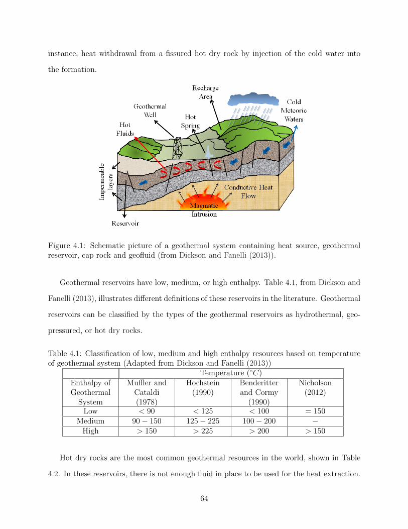
instance, heat withdrawal from a fissured hot dry rock by injection of the cold water into

the formation.

Figure 4.1: Schematic picture of a geothermal system containing heat source, geothermalreservoir, cap rock and geofluid (from Dickson and Fanelli (2013)).

Geothermal reservoirs have low, medium, or high enthalpy. Table 4.1, from Dickson and

Fanelli (2013), illustrates different definitions of these reservoirs in the literature. Geothermal

reservoirs can be classified by the types of the geothermal reservoirs as hydrothermal, geo-

pressured, or hot dry rocks.

Table 4.1: Classification of low, medium and high enthalpy resources based on temperatureof geothermal system (Adapted from Dickson and Fanelli (2013))

Temperature (C)Enthalpy ofGeothermal

System

Muffler andCataldi(1978)

Hochstein(1990)

Benderitterand Cormy

(1990)

Nicholson(2012)

Low < 90 < 125 < 100 = 150Medium 90− 150 125− 225 100− 200 −

High > 150 > 225 > 200 > 150

Hot dry rocks are the most common geothermal resources in the world, shown in Table

4.2. In these reservoirs, there is not enough fluid in place to be used for the heat extraction.

64

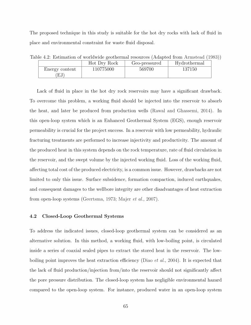
The proposed technique in this study is suitable for the hot dry rocks with lack of fluid in

place and environmental constraint for waste fluid disposal.

Table 4.2: Estimation of worldwide geothermal resources (Adapted from Armstead (1983))Hot Dry Rock Geo-pressured Hydrothermal

Energy content(EJ)

110775000 569700 137150

Lack of fluid in place in the hot dry rock reservoirs may have a significant drawback.

To overcome this problem, a working fluid should be injected into the reservoir to absorb

the heat, and later be produced from production wells (Rawal and Ghassemi, 2014). In

this open-loop system which is an Enhanced Geothermal System (EGS), enough reservoir

permeability is crucial for the project success. In a reservoir with low permeability, hydraulic

fracturing treatments are performed to increase injectivity and productivity. The amount of

the produced heat in this system depends on the rock temperature, rate of fluid circulation in

the reservoir, and the swept volume by the injected working fluid. Loss of the working fluid,

affecting total cost of the produced electricity, is a common issue. However, drawbacks are not

limited to only this issue. Surface subsidence, formation compaction, induced earthquakes,

and consequent damages to the wellbore integrity are other disadvantages of heat extraction

from open-loop systems (Geertsma, 1973; Majer et al., 2007).

4.2 Closed-Loop Geothermal Systems

To address the indicated issues, closed-loop geothermal system can be considered as an

alternative solution. In this method, a working fluid, with low-boiling point, is circulated

inside a series of coaxial sealed pipes to extract the stored heat in the reservoir. The low-

boiling point improves the heat extraction efficiency (Diao et al., 2004). It is expected that

the lack of fluid production/injection from/into the reservoir should not significantly affect

the pore pressure distribution. The closed-loop system has negligible environmental hazard

compared to the open-loop system. For instance, produced water in an open-loop system

65

contains high levels of sulfur, salt, and radioactive elements. Therefore, extracted water

should be injected back into the reservoir which is a costly process (Kagel et al., 2005).

Land subsidence is another drawback in the open-loop systems. Production of the ground

water reduces the pore pressure. Most of the open-loop facilities address this problem with

reinjection of the working fluid into the reservoir; however, this solution can induce significant

seismic events. For instance, induced earthquakes in an open-loop geothermal plant in Basel,

Switzerland, led to suspension of the whole project (Giardini, 2009).

Focus of the present study is on enhancing heat extraction from a closed-loop geothermal

wellbore via thermal conductive fractures. A thermoporoelastic finite element model is

developed to study the geomechanical behavior of the proposed system as well as heat

production. Thermoporoelasticity enables us to couple temperature, pore pressure, and

displacement changes in the reservoir especially close to the wellbore. To solve the governing

partial differential equations, Finite Element Method (FEM) is used to solve the governing

equations.

In classic closed-loop systems, heat transfer is mainly limited to the area close to the

wellbore. However, mere conduction cannot withdraw enough energy from the geothermal

reservoir to keep the heat production economically feasible. To address this deficiency,

somehow the formation-wellbore contact area as well as the conductivity of the area around

the wellbore should be increased. To improve the conductivity in the vicinity of the wellbore

and to minimize the heat loss, high conductivity cements can be used (Xu and Chung,

2000; Dahi Taleghani, 2013). Hydraulic fracturing of geothermal wells can improve the

formation-wellbore contact area and may increase the rate of heat extraction. Figure 4.2

depicts a horizontal wellbore connected to a double-wing vertical fracture. The induced

fracture is filled by the proppants with significantly larger thermal conductivity than the

thermal conductivity of the rock matrix. The conductive fracture acts as a thermal conduit

to transfer the heat from the reservoir into the wellbore.

66

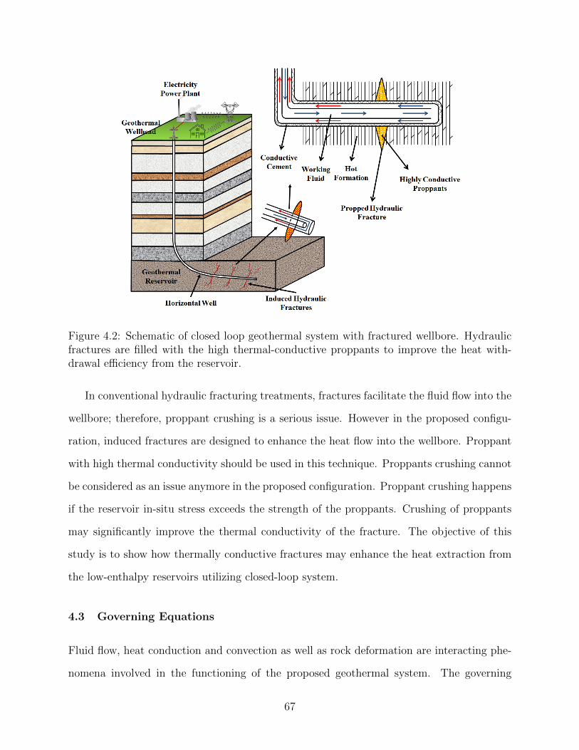
Figure 4.2: Schematic of closed loop geothermal system with fractured wellbore. Hydraulicfractures are filled with the high thermal-conductive proppants to improve the heat with-drawal efficiency from the reservoir.

In conventional hydraulic fracturing treatments, fractures facilitate the fluid flow into the

wellbore; therefore, proppant crushing is a serious issue. However in the proposed configu-

ration, induced fractures are designed to enhance the heat flow into the wellbore. Proppant

with high thermal conductivity should be used in this technique. Proppants crushing cannot

be considered as an issue anymore in the proposed configuration. Proppant crushing happens

if the reservoir in-situ stress exceeds the strength of the proppants. Crushing of proppants

may significantly improve the thermal conductivity of the fracture. The objective of this

study is to show how thermally conductive fractures may enhance the heat extraction from

the low-enthalpy reservoirs utilizing closed-loop system.

4.3 Governing Equations

Fluid flow, heat conduction and convection as well as rock deformation are interacting phe-

nomena involved in the functioning of the proposed geothermal system. The governing

67

equation of the thermo-hydro-mechanical problem can be obtained from the balance prin-

ciples. The displacement, pore pressure, and temperature are usually the primary solution

field stored at the nodal points. If the whole set of governing equations are solved simulta-

neously, then the solver is called monolithic. The monolithic solver is particularly important

for strongly coupled problems.

Porous media is void solid frame saturated with the geofluids. Interactions between

the solid grains, geofluids, and external forces dictate the relationship between fluid flow,

heat transfer, and mechanical behavior of the porous media. To analyze the behavior of

such a system, a multidisciplinary approach is required to couple the solid deformation

with the change in the pore pressure and the medium temperature. Change in the volume

of rock matrix comes from the rock expansion/contraction, induced by the temperature

rise/drop as well as fluid injection/production. The induced deformation, caused by the

rock contraction/expansion, may affect the reservoir storage capacity and its permeability.

In the literature, there are several analytical solutions to study the coupling of heat trans-

fer and fluid flow in deformable porous media (McTigue, 1986; Kodashima and Kurashige,

1996; Bai and Abousleiman, 1997; Belotserkovets and Prevost, 2011). However, these analyt-

ical solutions are derived for simple geometries with limited initial and boundary conditions,

and neglecting different terms in the governing equations. In contrast, numerical method is

more powerful and flexible to accurately approximate the solutions of realistic engineering

problems. For instance, McTigue (1986) decoupled the energy equation from the momentum

and mass balance equations. Kodashima and Kurashige (1996) did not consider the effect

of the thermo-poro-mechanical response on the displacement fields. Bai and Abousleiman

(1997) solved a thermo-poroelasticity problem for a one-dimensional geometry by dismissing

convection in their solution.

Any disturbance in the formation temperature or pore pressure can initiate deformation.

The deformation of a one-dimensional porous skeleton under loading was originally intro-

duced by the Terzaghi (1925). He studied the behaviors of fully saturated soils under a

68

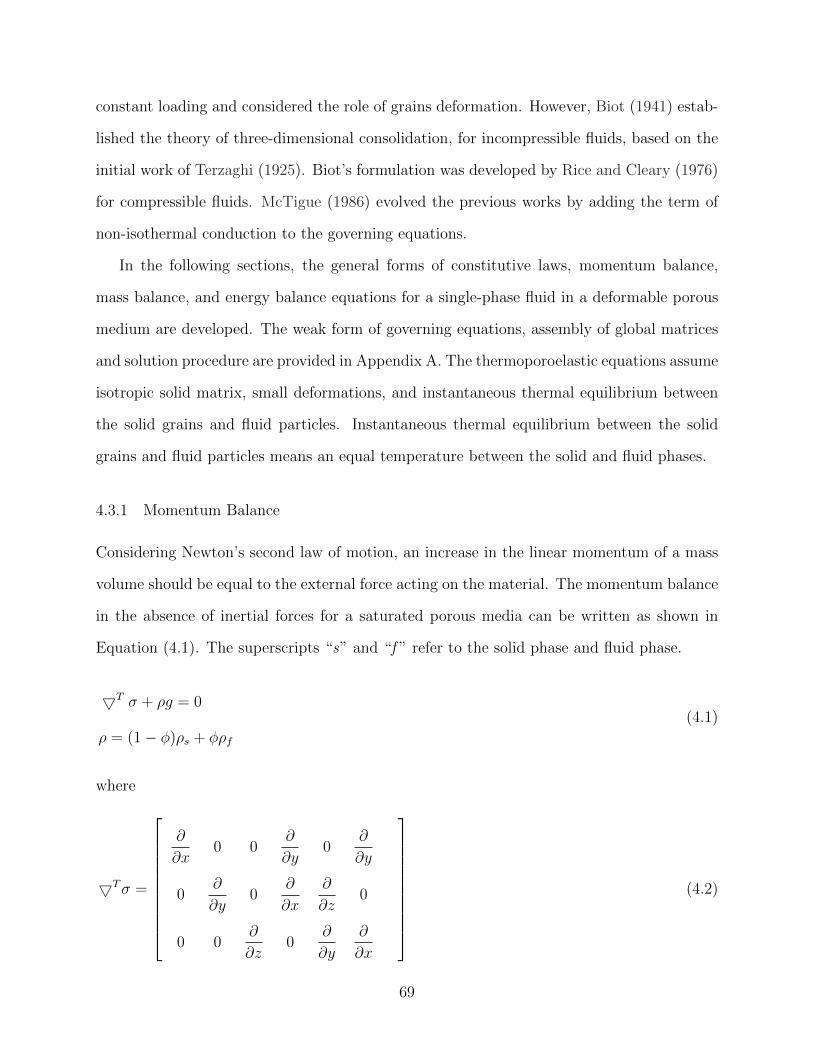
constant loading and considered the role of grains deformation. However, Biot (1941) estab-

lished the theory of three-dimensional consolidation, for incompressible fluids, based on the

initial work of Terzaghi (1925). Biot’s formulation was developed by Rice and Cleary (1976)

for compressible fluids. McTigue (1986) evolved the previous works by adding the term of

non-isothermal conduction to the governing equations.

In the following sections, the general forms of constitutive laws, momentum balance,

mass balance, and energy balance equations for a single-phase fluid in a deformable porous

medium are developed. The weak form of governing equations, assembly of global matrices

and solution procedure are provided in Appendix A. The thermoporoelastic equations assume

isotropic solid matrix, small deformations, and instantaneous thermal equilibrium between

the solid grains and fluid particles. Instantaneous thermal equilibrium between the solid

grains and fluid particles means an equal temperature between the solid and fluid phases.

4.3.1 Momentum Balance

Considering Newton’s second law of motion, an increase in the linear momentum of a mass

volume should be equal to the external force acting on the material. The momentum balance

in the absence of inertial forces for a saturated porous media can be written as shown in

Equation (4.1). The superscripts “s” and “f ” refer to the solid phase and fluid phase.

5T σ + ρg = 0

ρ = (1− φ)ρs + φρf

(4.1)

where

5Tσ =

∂

∂x0 0

∂

∂y0

∂

∂y

0∂

∂y0

∂

∂x

∂

∂z0

0 0∂

∂z0

∂

∂y

∂

∂x

(4.2)

69

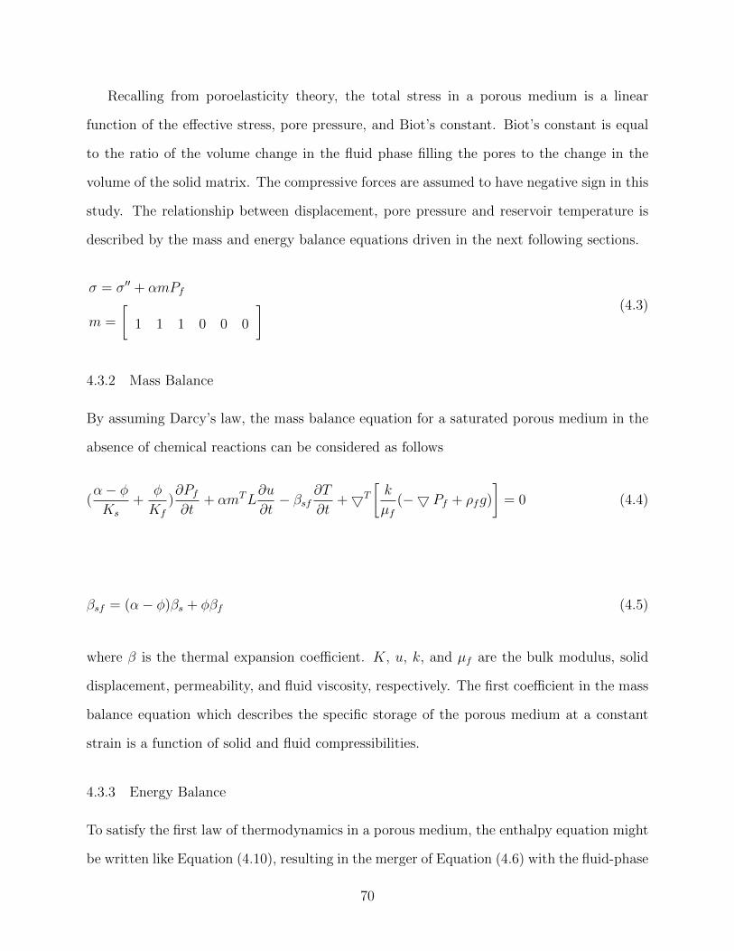
Recalling from poroelasticity theory, the total stress in a porous medium is a linear

function of the effective stress, pore pressure, and Biot’s constant. Biot’s constant is equal

to the ratio of the volume change in the fluid phase filling the pores to the change in the

volume of the solid matrix. The compressive forces are assumed to have negative sign in this

study. The relationship between displacement, pore pressure and reservoir temperature is

described by the mass and energy balance equations driven in the next following sections.

σ = σ′′ + αmPf

m =

[1 1 1 0 0 0

] (4.3)

4.3.2 Mass Balance

By assuming Darcy’s law, the mass balance equation for a saturated porous medium in the

absence of chemical reactions can be considered as follows

(α− φKs

+φ

Kf

)∂Pf∂t

+ αmTL∂u

∂t− βsf

∂T

∂t+5T

[k

µf(−5 Pf + ρfg)

]= 0 (4.4)

βsf = (α− φ)βs + φβf (4.5)

where β is the thermal expansion coefficient. K, u, k, and µf are the bulk modulus, solid

displacement, permeability, and fluid viscosity, respectively. The first coefficient in the mass

balance equation which describes the specific storage of the porous medium at a constant

strain is a function of solid and fluid compressibilities.

4.3.3 Energy Balance

To satisfy the first law of thermodynamics in a porous medium, the enthalpy equation might

be written like Equation (4.10), resulting in the merger of Equation (4.6) with the fluid-phase

70

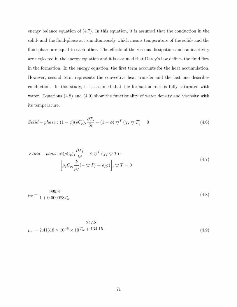
energy balance equation of (4.7). In this equation, it is assumed that the conduction in the

solid- and the fluid-phase act simultaneously which means temperature of the solid- and the

fluid-phase are equal to each other. The effects of the viscous dissipation and radioactivity

are neglected in the energy equation and it is assumed that Darcy’s law defines the fluid flow

in the formation. In the energy equation, the first term accounts for the heat accumulation.

However, second term represents the convective heat transfer and the last one describes

conduction. In this study, it is assumed that the formation rock is fully saturated with

water. Equations (4.8) and (4.9) show the functionality of water density and viscosity with

its temperature.

Solid− phase : (1− φ)(ρCp)s∂Ts∂t− (1− φ)5T (χs5 T ) = 0 (4.6)

Fluid− phase :φ(ρCp)f∂Tf∂t− φ5T (χf 5 T )+[

ρfCpfk

µf(−5 Pf + ρfg)

].5 T = 0

(4.7)

ρw =999.8

1 + 0.000088Tw(4.8)

µw = 2.41318× 10−5 × 10

247.8

Tw + 134.15 (4.9)

71

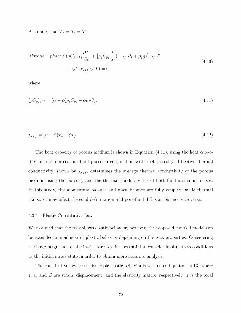
Assuming that Tf = Ts = T

Porous− phase : (ρCp)eff∂Ts∂t

+[ρfCpf

k

µf(−5 Pf + ρfg)

].5 T

−5T (χeff 5 T ) = 0

(4.10)

where

(ρCp)eff = (α− φ)ρsCps + φρfCpf (4.11)

χeff = (α− φ)χs + φχf (4.12)

The heat capacity of porous medium is shown in Equation (4.11), using the heat capac-

ities of rock matrix and fluid phase in conjunction with rock porosity. Effective thermal

conductivity, shown by χeff , determines the average thermal conductivity of the porous

medium using the porosity and the thermal conductivities of both fluid and solid phases.

In this study, the momentum balance and mass balance are fully coupled, while thermal

transport may affect the solid deformation and pore-fluid diffusion but not vice versa.

4.3.4 Elastic Constitutive Law

We assumed that the rock shows elastic behavior; however, the proposed coupled model can

be extended to nonlinear or plastic behavior depending on the rock properties. Considering

the large magnitude of the in-situ stresses, it is essential to consider in-situ stress conditions

as the initial stress state in order to obtain more accurate analysis.

The constitutive law for the isotropic elastic behavior is written as Equation (4.13) where

ε, u, and D are strain, displacement, and the elasticity matrix, respectively. ε is the total

72

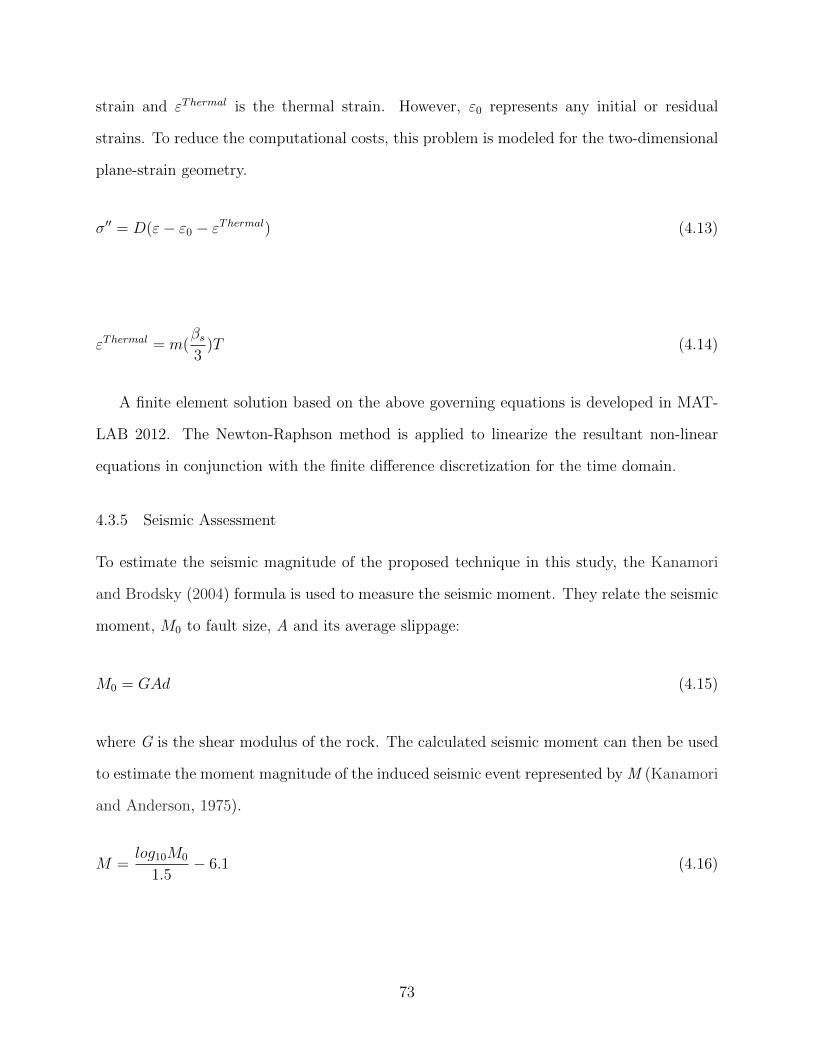
strain and εThermal is the thermal strain. However, ε0 represents any initial or residual

strains. To reduce the computational costs, this problem is modeled for the two-dimensional

plane-strain geometry.

σ′′ = D(ε− ε0 − εThermal) (4.13)

εThermal = m(βs3

)T (4.14)

A finite element solution based on the above governing equations is developed in MAT-

LAB 2012. The Newton-Raphson method is applied to linearize the resultant non-linear

equations in conjunction with the finite difference discretization for the time domain.

4.3.5 Seismic Assessment

To estimate the seismic magnitude of the proposed technique in this study, the Kanamori

and Brodsky (2004) formula is used to measure the seismic moment. They relate the seismic

moment, M0 to fault size, A and its average slippage:

M0 = GAd (4.15)

where G is the shear modulus of the rock. The calculated seismic moment can then be used

to estimate the moment magnitude of the induced seismic event represented by M (Kanamori

and Anderson, 1975).

M =log10M0

1.5− 6.1 (4.16)

73

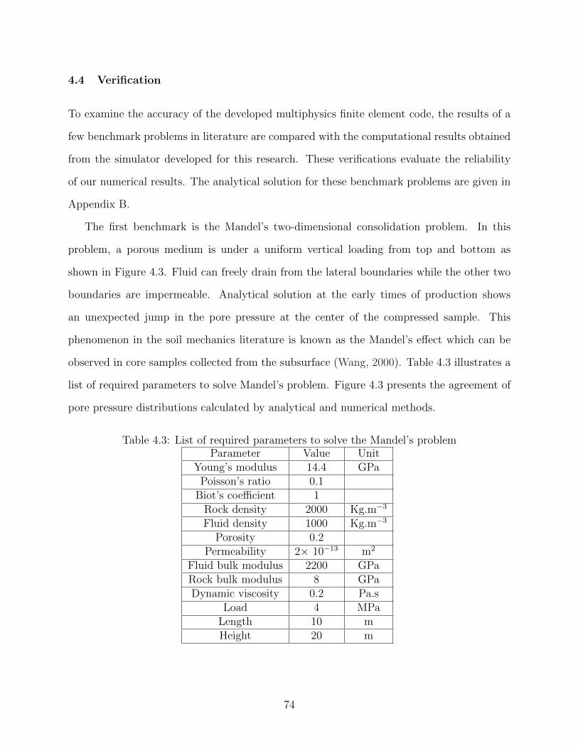
4.4 Verification

To examine the accuracy of the developed multiphysics finite element code, the results of a

few benchmark problems in literature are compared with the computational results obtained

from the simulator developed for this research. These verifications evaluate the reliability

of our numerical results. The analytical solution for these benchmark problems are given in

Appendix B.

The first benchmark is the Mandel’s two-dimensional consolidation problem. In this

problem, a porous medium is under a uniform vertical loading from top and bottom as

shown in Figure 4.3. Fluid can freely drain from the lateral boundaries while the other two

boundaries are impermeable. Analytical solution at the early times of production shows

an unexpected jump in the pore pressure at the center of the compressed sample. This

phenomenon in the soil mechanics literature is known as the Mandel’s effect which can be

observed in core samples collected from the subsurface (Wang, 2000). Table 4.3 illustrates a

list of required parameters to solve Mandel’s problem. Figure 4.3 presents the agreement of

pore pressure distributions calculated by analytical and numerical methods.

Table 4.3: List of required parameters to solve the Mandel’s problemParameter Value Unit

Young’s modulus 14.4 GPaPoisson’s ratio 0.1

Biot’s coefficient 1Rock density 2000 Kg.m−3

Fluid density 1000 Kg.m−3

Porosity 0.2Permeability 2× 10−13 m2

Fluid bulk modulus 2200 GPaRock bulk modulus 8 GPaDynamic viscosity 0.2 Pa.s

Load 4 MPaLength 10 mHeight 20 m

74

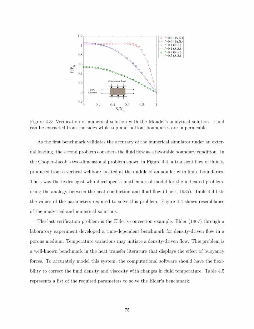
Figure 4.3: Verification of numerical solution with the Mandel’s analytical solution. Fluidcan be extracted from the sides while top and bottom boundaries are impermeable.

As the first benchmark validates the accuracy of the numerical simulator under an exter-

nal loading, the second problem considers the fluid flow as a favorable boundary condition. In

the Cooper-Jacob’s two-dimensional problem shown in Figure 4.4, a transient flow of fluid is

produced from a vertical wellbore located at the middle of an aquifer with finite boundaries.

Theis was the hydrologist who developed a mathematical model for the indicated problem,

using the analogy between the heat conduction and fluid flow (Theis, 1935). Table 4.4 lists

the values of the parameters required to solve this problem. Figure 4.4 shows resemblance

of the analytical and numerical solutions.

The last verification problem is the Elder’s convection example. Elder (1967) through a

laboratory experiment developed a time-dependent benchmark for density-driven flow in a

porous medium. Temperature variations may initiate a density-driven flow. This problem is

a well-known benchmark in the heat transfer literature that displays the effect of buoyancy

forces. To accurately model this system, the computational software should have the flexi-

bility to correct the fluid density and viscosity with changes in fluid temperature. Table 4.5

represents a list of the required parameters to solve the Elder’s benchmark.

75

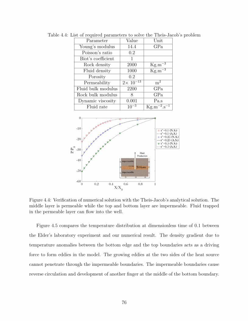
Table 4.4: List of required parameters to solve the Theis-Jacob’s problemParameter Value Unit

Young’s modulus 14.4 GPaPoisson’s ratio 0.2

Biot’s coefficient 1Rock density 2000 Kg.m−3

Fluid density 1000 Kg.m−3

Porosity 0.2Permeability 2× 10−13 m2

Fluid bulk modulus 2200 GPaRock bulk modulus 8 GPaDynamic viscosity 0.001 Pa.s

Fluid rate 10−3 Kg.m−2.s−1

Figure 4.4: Verification of numerical solution with the Theis-Jacob’s analytical solution. Themiddle layer is permeable while the top and bottom layer are impermeable. Fluid trappedin the permeable layer can flow into the well.

Figure 4.5 compares the temperature distribution at dimensionless time of 0.1 between

the Elder’s laboratory experiment and our numerical result. The density gradient due to

temperature anomalies between the bottom edge and the top boundaries acts as a driving

force to form eddies in the model. The growing eddies at the two sides of the heat source

cannot penetrate through the impermeable boundaries. The impermeable boundaries cause

reverse circulation and development of another finger at the middle of the bottom boundary.

76

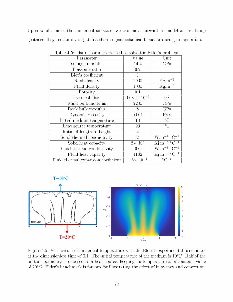
Upon validation of the numerical software, we can move forward to model a closed-loop

geothermal system to investigate its thermo-geomechanical behavior during its operation.

Table 4.5: List of parameters used to solve the Elder’s problemParameter Value Unit

Young’s modulus 14.4 GPaPoisson’s ratio 0.2

Biot’s coefficient 1Rock density 2000 Kg.m−3

Fluid density 1000 Kg.m−3

Porosity 0.1Permeability 9.084× 10−9 m2

Fluid bulk modulus 2200 GPaRock bulk modulus 8 GPaDynamic viscosity 0.001 Pa.s

Initial medium temperature 10 CHeat source temperature 20 CRatio of length to height 4

Solid thermal conductivity 2 W.m−1 C−1

Solid heat capacity 2× 103 Kj.m−3 C−1

Fluid thermal conductivity 0.6 W.m−1 C−1

Fluid heat capacity 4182 Kj.m−3 C−1

Fluid thermal expansion coefficient 1.5× 10−4 C−1

Figure 4.5: Verification of numerical temperature with the Elder’s experimental benchmarkat the dimensionless time of 0.1. The initial temperature of the medium is 10C. Half of thebottom boundary is exposed to a heat source, keeping its temperature at a constant valueof 20C. Elder’s benchmark is famous for illustrating the effect of buoyancy and convection.

77

4.5 Results and Discussion

Drastic climate changes during the last century caused by the emission of greenhouse gases

from the burning fossil fuels has encouraged countries to expand the application of clean and

sustainable energy resources. Geothermal energy is one of these sustainable resources and

the general interest in the production of electricity from the geothermal power plants has

immensely risen in recent years. The aim of the present study is to illustrate how induced

hydraulic fractures filled with the highly thermal-conductive proppants may enhance the

efficiency of heat withdrawal in the closed-loop systems as a new technique. The surface

subsidence and seismic hazards involved in the heat production from the geothermal systems

are studied through executing a coupled finite element simulation.

Drilling a well has a significant share in the overall costs of a geothermal project. To

reduce the project costs, existing abandoned wells in the areas with sufficient temperature

gradient can be converted into the geothermal wells. A candidate reservoir in the United

States with several abandoned oil and gas wells can be found in Camerina A formation.

Camerina A is a geopressured formation located in South Louisiana, at the border of Ver-

million and Acadia Parishes. Camerina A formation located at the depth of 4000 meters

below the ground surface has a thickness of 200 to 400 meters at different locations. Kehle

(1973) estimated a temperature gradient of 28 to 30C per kilometer along the sand layer

of this formation. Recalling the Nicholson’s definition from Table 4.1, this formation can

be categorized as a low-enthalpy geothermal reservoir. Numerical simulations in this study

are executed for a reservoir with the similar rock-fluid-physical properties as Camerina A

formation. Table 4.6 summarizes all of the properties required to model heat withdrawal

from the proposed geothermal system described in Figure 4.2 (Gray, 2010).

To model the heat transfer and fluid flow along with the mechanical behavior of the

rock matrix, a fully coupled two-dimensional finite element model is developed to represent

the heat withdrawal from a horizontal wellbore connected to a vertical induced fracture.

78

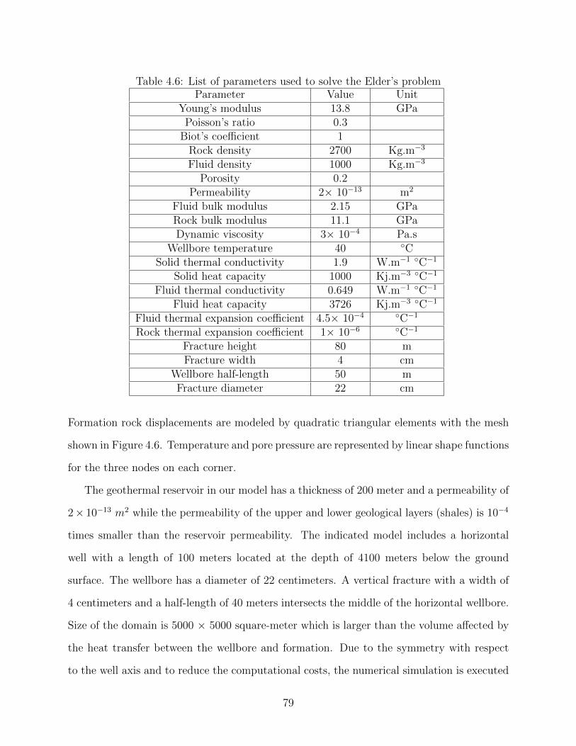
Table 4.6: List of parameters used to solve the Elder’s problemParameter Value Unit

Young’s modulus 13.8 GPaPoisson’s ratio 0.3

Biot’s coefficient 1Rock density 2700 Kg.m−3

Fluid density 1000 Kg.m−3

Porosity 0.2Permeability 2× 10−13 m2

Fluid bulk modulus 2.15 GPaRock bulk modulus 11.1 GPaDynamic viscosity 3× 10−4 Pa.s

Wellbore temperature 40 CSolid thermal conductivity 1.9 W.m−1 C−1

Solid heat capacity 1000 Kj.m−3 C−1

Fluid thermal conductivity 0.649 W.m−1 C−1

Fluid heat capacity 3726 Kj.m−3 C−1

Fluid thermal expansion coefficient 4.5× 10−4 C−1

Rock thermal expansion coefficient 1× 10−6 C−1

Fracture height 80 mFracture width 4 cm

Wellbore half-length 50 mFracture diameter 22 cm

Formation rock displacements are modeled by quadratic triangular elements with the mesh

shown in Figure 4.6. Temperature and pore pressure are represented by linear shape functions

for the three nodes on each corner.

The geothermal reservoir in our model has a thickness of 200 meter and a permeability of

2× 10−13 m2 while the permeability of the upper and lower geological layers (shales) is 10−4

times smaller than the reservoir permeability. The indicated model includes a horizontal

well with a length of 100 meters located at the depth of 4100 meters below the ground

surface. The wellbore has a diameter of 22 centimeters. A vertical fracture with a width of

4 centimeters and a half-length of 40 meters intersects the middle of the horizontal wellbore.

Size of the domain is 5000 × 5000 square-meter which is larger than the volume affected by

the heat transfer between the wellbore and formation. Due to the symmetry with respect

to the well axis and to reduce the computational costs, the numerical simulation is executed

79

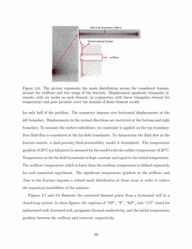
Figure 4.6: The picture represents the mesh distribution across the considered domain,around the wellbore and two wings of the fracture. Displacement quadratic triangular el-ements, with six nodes on each element, in conjunction with linear triangular element fortemperature and pore pressure cover the domain of finite element model.

for only half of the problem. The symmetry imposes zero horizontal displacements at the

left boundary. Displacements in the normal directions are restricted at the bottom and right

boundary. To measure the surface subsidence, no constraint is applied on the top boundary.

Zero fluid-flux is considered at the far-field boundaries. To characterize the fluid flow in the

fracture-matrix, a dual-porosity/dual-permeability model is formulated. The temperature

gradient of 28C per kilometer is assumed for the model with the surface temperature of 20C.

Temperature at the far-field boundaries is kept constant and equal to the initial temperature.

The wellbore temperature which is lower than the medium temperature is defined separately

for each numerical experiment. The significant temperature gradient at the wellbore and

close to the fracture imposes a refined mesh distribution at those areas in order to reduce

the numerical instabilities of the solution.

Figures 4.7 and 4.8 illustrate the extracted thermal power from a horizontal well in a

closed-loop system. In these figures, the captions of “NF”, “F”, “KP”, and “4T” stand for

unfractured well, fractured well, proppants thermal conductivity, and the initial temperature

gradient between the wellbore and reservoir, respectively.

80

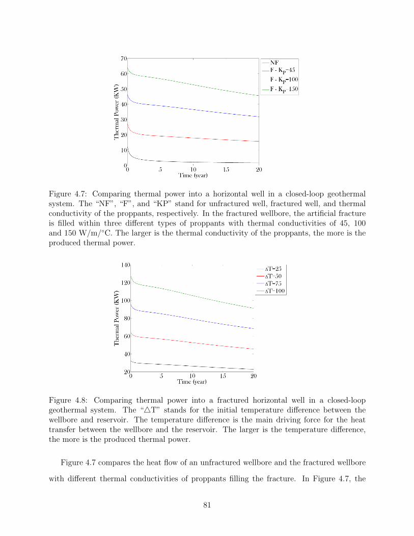
Figure 4.7: Comparing thermal power into a horizontal well in a closed-loop geothermalsystem. The “NF”, “F”, and “KP” stand for unfractured well, fractured well, and thermalconductivity of the proppants, respectively. In the fractured wellbore, the artificial fractureis filled within three different types of proppants with thermal conductivities of 45, 100and 150 W/m/C. The larger is the thermal conductivity of the proppants, the more is theproduced thermal power.

Figure 4.8: Comparing thermal power into a fractured horizontal well in a closed-loopgeothermal system. The “4T” stands for the initial temperature difference between thewellbore and reservoir. The temperature difference is the main driving force for the heattransfer between the wellbore and the reservoir. The larger is the temperature difference,the more is the produced thermal power.

Figure 4.7 compares the heat flow of an unfractured wellbore and the fractured wellbore

with different thermal conductivities of proppants filling the fracture. In Figure 4.7, the

81

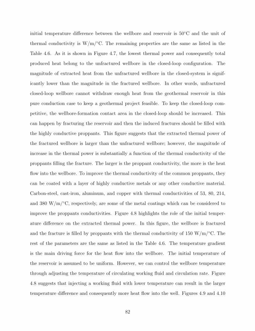
initial temperature difference between the wellbore and reservoir is 50C and the unit of

thermal conductivity is W/m/C. The remaining properties are the same as listed in the

Table 4.6. As it is shown in Figure 4.7, the lowest thermal power and consequently total

produced heat belong to the unfractured wellbore in the closed-loop configuration. The

magnitude of extracted heat from the unfractured wellbore in the closed-system is signif-

icantly lower than the magnitude in the fractured wellbore. In other words, unfractured

closed-loop wellbore cannot withdraw enough heat from the geothermal reservoir in this

pure conduction case to keep a geothermal project feasible. To keep the closed-loop com-

petitive, the wellbore-formation contact area in the closed-loop should be increased. This

can happen by fracturing the reservoir and then the induced fractures should be filled with

the highly conductive proppants. This figure suggests that the extracted thermal power of

the fractured wellbore is larger than the unfractured wellbore; however, the magnitude of

increase in the thermal power is substantially a function of the thermal conductivity of the

proppants filling the fracture. The larger is the proppant conductivity, the more is the heat

flow into the wellbore. To improve the thermal conductivity of the common proppants, they

can be coated with a layer of highly conductive metals or any other conductive material.

Carbon-steel, cast-iron, aluminum, and copper with thermal conductivities of 53, 80, 214,

and 380 W/m/C, respectively, are some of the metal coatings which can be considered to

improve the proppants conductivities. Figure 4.8 highlights the role of the initial temper-

ature difference on the extracted thermal power. In this figure, the wellbore is fractured

and the fracture is filled by proppants with the thermal conductivity of 150 W/m/C. The

rest of the parameters are the same as listed in the Table 4.6. The temperature gradient

is the main driving force for the heat flow into the wellbore. The initial temperature of

the reservoir is assumed to be uniform. However, we can control the wellbore temperature

through adjusting the temperature of circulating working fluid and circulation rate. Figure

4.8 suggests that injecting a working fluid with lower temperature can result in the larger

temperature difference and consequently more heat flow into the well. Figures 4.9 and 4.10

82

compare the magnitude of cumulative extracted heat during a time span of 20 years for the

Figures 4.7 and 4.8, respectively. Figures 4.9 and 4.10 emphasize that connecting a wellbore

to highly conductive fractures as well as enforcing a considerable temperature gradient can

improve the extracted heat in the closed-loop geothermal systems.

Figure 4.9: Comparing cumulative extracted heat from a horizontal well in a closed-loopgeothermal system. The cumulative collected heat for the wellbore with the fracture filledwithin the high thermal conductive proppants is one order of magnitude larger than theunfractured wellbore.

Figure 4.10: Comparing cumulative extracted heat from a horizontal well in a closed-loopgeothermal system. This Figure suggest that the increase in the temperature difference cansignificantly improve the extracted heat.

83

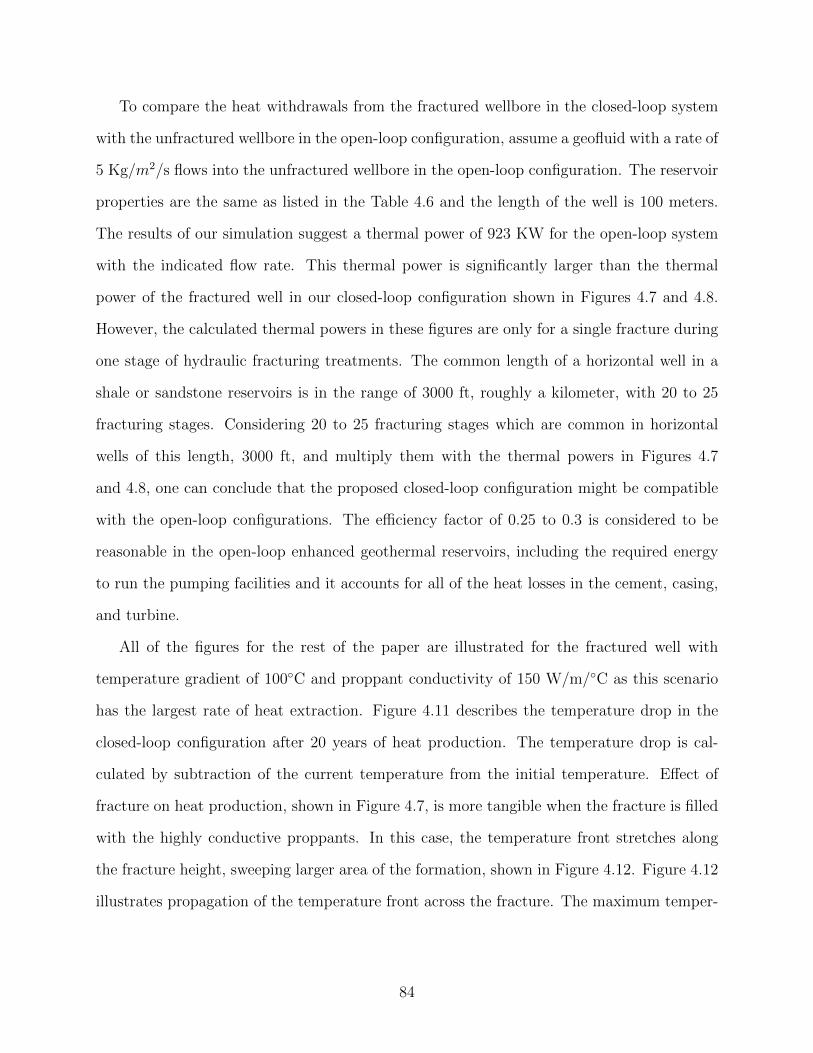
To compare the heat withdrawals from the fractured wellbore in the closed-loop system

with the unfractured wellbore in the open-loop configuration, assume a geofluid with a rate of

5 Kg/m2/s flows into the unfractured wellbore in the open-loop configuration. The reservoir

properties are the same as listed in the Table 4.6 and the length of the well is 100 meters.

The results of our simulation suggest a thermal power of 923 KW for the open-loop system

with the indicated flow rate. This thermal power is significantly larger than the thermal

power of the fractured well in our closed-loop configuration shown in Figures 4.7 and 4.8.

However, the calculated thermal powers in these figures are only for a single fracture during

one stage of hydraulic fracturing treatments. The common length of a horizontal well in a

shale or sandstone reservoirs is in the range of 3000 ft, roughly a kilometer, with 20 to 25

fracturing stages. Considering 20 to 25 fracturing stages which are common in horizontal

wells of this length, 3000 ft, and multiply them with the thermal powers in Figures 4.7

and 4.8, one can conclude that the proposed closed-loop configuration might be compatible

with the open-loop configurations. The efficiency factor of 0.25 to 0.3 is considered to be

reasonable in the open-loop enhanced geothermal reservoirs, including the required energy

to run the pumping facilities and it accounts for all of the heat losses in the cement, casing,

and turbine.

All of the figures for the rest of the paper are illustrated for the fractured well with

temperature gradient of 100C and proppant conductivity of 150 W/m/C as this scenario

has the largest rate of heat extraction. Figure 4.11 describes the temperature drop in the

closed-loop configuration after 20 years of heat production. The temperature drop is cal-

culated by subtraction of the current temperature from the initial temperature. Effect of

fracture on heat production, shown in Figure 4.7, is more tangible when the fracture is filled

with the highly conductive proppants. In this case, the temperature front stretches along

the fracture height, sweeping larger area of the formation, shown in Figure 4.12. Figure 4.12

illustrates propagation of the temperature front across the fracture. The maximum temper-

84

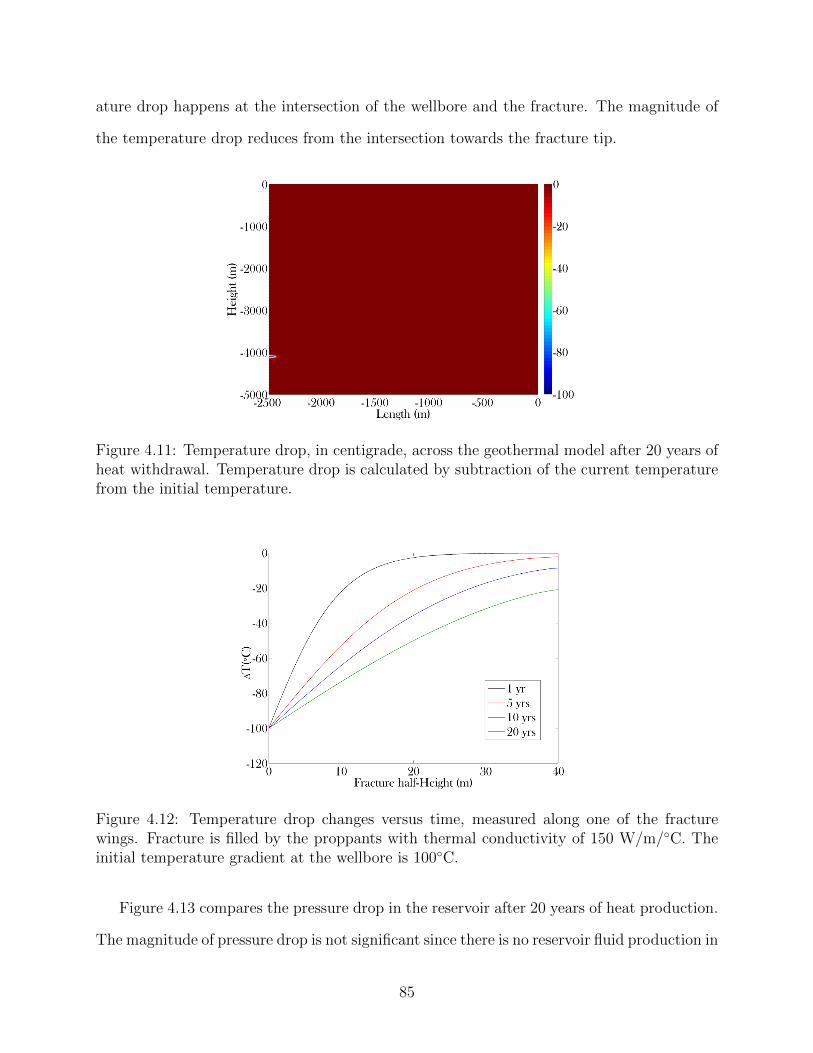
ature drop happens at the intersection of the wellbore and the fracture. The magnitude of

the temperature drop reduces from the intersection towards the fracture tip.

Figure 4.11: Temperature drop, in centigrade, across the geothermal model after 20 years ofheat withdrawal. Temperature drop is calculated by subtraction of the current temperaturefrom the initial temperature.

Figure 4.12: Temperature drop changes versus time, measured along one of the fracturewings. Fracture is filled by the proppants with thermal conductivity of 150 W/m/C. Theinitial temperature gradient at the wellbore is 100C.

Figure 4.13 compares the pressure drop in the reservoir after 20 years of heat production.

The magnitude of pressure drop is not significant since there is no reservoir fluid production in

85

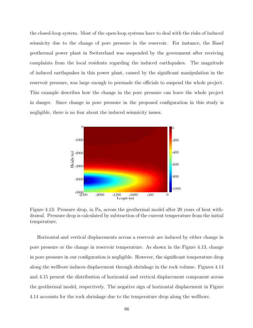
the closed-loop system. Most of the open-loop systems have to deal with the risks of induced

seismicity due to the change of pore pressure in the reservoir. For instance, the Basel

geothermal power plant in Switzerland was suspended by the government after receiving

complaints from the local residents regarding the induced earthquakes. The magnitude

of induced earthquakes in this power plant, caused by the significant manipulation in the

reservoir pressure, was large enough to persuade the officials to suspend the whole project.

This example describes how the change in the pore pressure can leave the whole project

in danger. Since change in pore pressure in the proposed configuration in this study is

negligible, there is no fear about the induced seismicity issues.

Figure 4.13: Pressure drop, in Pa, across the geothermal model after 20 years of heat with-drawal. Pressure drop is calculated by subtraction of the current temperature from the initialtemperature.

Horizontal and vertical displacements across a reservoir are induced by either change in

pore pressure or the change in reservoir temperature. As shown in the Figure 4.13, change

in pore pressure in our configuration is negligible. However, the significant temperature drop

along the wellbore induces displacement through shrinkage in the rock volume. Figures 4.14

and 4.15 present the distribution of horizontal and vertical displacement component across

the geothermal model, respectively. The negative sign of horizontal displacement in Figure

4.14 accounts for the rock shrinkage due to the temperature drop along the wellbore.

86

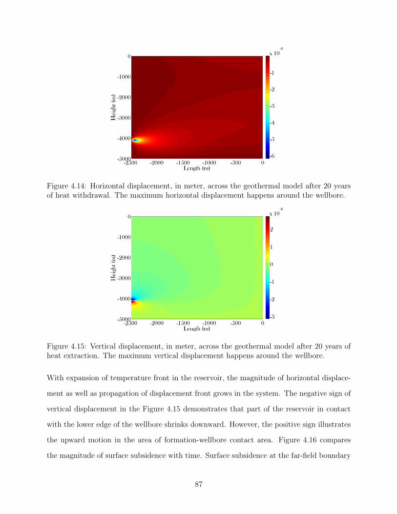
Figure 4.14: Horizontal displacement, in meter, across the geothermal model after 20 yearsof heat withdrawal. The maximum horizontal displacement happens around the wellbore.

Figure 4.15: Vertical displacement, in meter, across the geothermal model after 20 years ofheat extraction. The maximum vertical displacement happens around the wellbore.

With expansion of temperature front in the reservoir, the magnitude of horizontal displace-

ment as well as propagation of displacement front grows in the system. The negative sign of

vertical displacement in the Figure 4.15 demonstrates that part of the reservoir in contact

with the lower edge of the wellbore shrinks downward. However, the positive sign illustrates

the upward motion in the area of formation-wellbore contact area. Figure 4.16 compares

the magnitude of surface subsidence with time. Surface subsidence at the far-field boundary

87

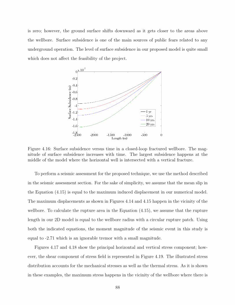
is zero; however, the ground surface shifts downward as it gets closer to the areas above

the wellbore. Surface subsidence is one of the main sources of public fears related to any

underground operation. The level of surface subsidence in our proposed model is quite small

which does not affect the feasibility of the project.

Figure 4.16: Surface subsidence versus time in a closed-loop fractured wellbore. The mag-nitude of surface subsidence increases with time. The largest subsidence happens at themiddle of the model where the horizontal well is intersected with a vertical fracture.

To perform a seismic assessment for the proposed technique, we use the method described

in the seismic assessment section. For the sake of simplicity, we assume that the mean slip in

the Equation (4.15) is equal to the maximum induced displacement in our numerical model.

The maximum displacements as shown in Figures 4.14 and 4.15 happen in the vicinity of the

wellbore. To calculate the rupture area in the Equation (4.15), we assume that the rupture

length in our 2D model is equal to the wellbore radius with a circular rupture patch. Using

both the indicated equations, the moment magnitude of the seismic event in this study is

equal to -2.71 which is an ignorable tremor with a small magnitude.

Figures 4.17 and 4.18 show the principal horizontal and vertical stress component; how-

ever, the shear component of stress field is represented in Figure 4.19. The illustrated stress

distribution accounts for the mechanical stresses as well as the thermal stress. As it is shown

in these examples, the maximum stress happens in the vicinity of the wellbore where there is

88

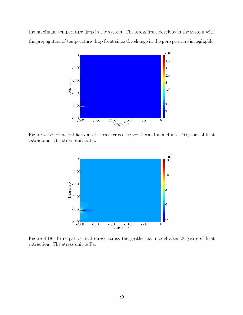
the maximum temperature drop in the system. The stress front develops in the system with

the propagation of temperature-drop front since the change in the pore pressure is negligible.

Figure 4.17: Principal horizontal stress across the geothermal model after 20 years of heatextraction. The stress unit is Pa.

Figure 4.18: Principal vertical stress across the geothermal model after 20 years of heatextraction. The stress unit is Pa.

89

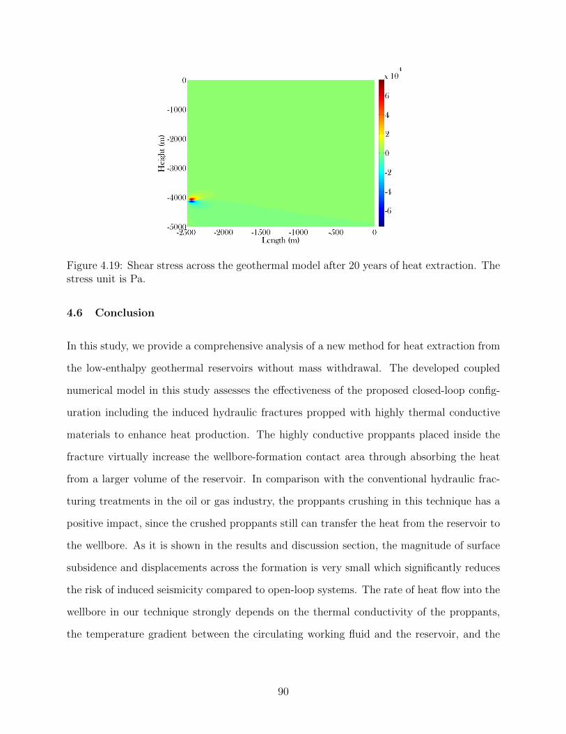
Figure 4.19: Shear stress across the geothermal model after 20 years of heat extraction. Thestress unit is Pa.

4.6 Conclusion

In this study, we provide a comprehensive analysis of a new method for heat extraction from

the low-enthalpy geothermal reservoirs without mass withdrawal. The developed coupled

numerical model in this study assesses the effectiveness of the proposed closed-loop config-

uration including the induced hydraulic fractures propped with highly thermal conductive

materials to enhance heat production. The highly conductive proppants placed inside the

fracture virtually increase the wellbore-formation contact area through absorbing the heat

from a larger volume of the reservoir. In comparison with the conventional hydraulic frac-

turing treatments in the oil or gas industry, the proppants crushing in this technique has a

positive impact, since the crushed proppants still can transfer the heat from the reservoir to

the wellbore. As it is shown in the results and discussion section, the magnitude of surface

subsidence and displacements across the formation is very small which significantly reduces

the risk of induced seismicity compared to open-loop systems. The rate of heat flow into the

wellbore in our technique strongly depends on the thermal conductivity of the proppants,

the temperature gradient between the circulating working fluid and the reservoir, and the

90

magnitude of increase in the wellbore-formation contact area. The numerical simulations

show promising economic value for the application of this technique to horizontal wellbores.

4.7 References

Armstead, H. C. H. “Geothermal energy: Its past, present, and future contributions to theenergy needs of man E. and FN Spon.” London, UK (1983).

Bai, M., and Y. Abousleiman. “Thermoporoelastic coupling with application to consolida-tion” International Journal for Numerical and Analytical Methods in Geomechanics: 21.2(1997): 121-132.

Belotserkovets, A., and J. H. Prevost. “Thermoporoelastic response of a fluid-saturatedporous sphere: An analytical solution.” International Journal of Engineering Science:49.12 (2011): 1415-1423.

Benderitter, Y., and G. Cormy. “Possible approach to geothermal research and relative costs”Small geothermal resources: A guide to development and utilization, UNITAR, New York(1990): 59-69.

Biot, M. A. “General theory of threedimensional consolidation.” Journal of applied physics12.2 (1941): 155-164.

Dahi Taleghani, A. “An Improved Closed-Loop Heat Extraction Method from GeothermalResources” Journal of Energy Resources Technology 135.4 (2013): 042904.

Diao, N., Q. Li, and Z. Fang. “Heat transfer in ground heat exchangers with groundwateradvection.” International Journal of Thermal Sciences 43.12 (2004): 1203-1211.

Dickson, M. H., and M. Fanelli. “Geothermal energy: utilization and technology.” Routledge,2013.

Duffield, W. A., and J. H. Sass. “Geothermal energy: Clean power from the earth’s heat.Diane Publishing: Vol. 1249. (2003).

Elder, J.W. “Transient convection in a porous medium. Journal of Fluid Mechanics, v. 27,no. 3, p. 609-623 (1967).

Feng, Yin, M. Tyagi, and C. D. White. “A downhole heat exchanger for horizontal wells inlow-enthalpy geopressured geothermal brine reservoirs.” Geothermics 53 (2015): 368-378.

Fridleifsson, I. B., R. Bertani, E. Huenges, J. W. Lund, A. Ragnarsson, and L. Rybach, “Thepossible role and contribution of geothermal energy to the mitigation of climate change.”IPCC scoping meeting on renewable energy sources, proceedings, Luebeck, Germany. Vol.20. No. 25. (2008).

91

Gray, T.A., “Geothermal resource assessment of the Gueydan salt dome and the adjacentsoutheast Gueydan field. Masters thesis, Louisiana State University, Baton Rouge, LA(2010).

Geertsma, J. “Land subsidence above compacting oil and gas reservoirs” Journal ofPetroleum Technology 25.6 (1973): 734-744.

Giardini, D. “Geothermal quake risks must be faced” Nature 462.7275 (2009): 848-849.

Hochstein, M. P. “Classification and assessment of geothermal resources” Small geothermalresources: A guide to development and utilization, UNITAR, New York (1990): 31-57.

Holm, A., D. Jennejohn, and L. Blodgett. “Geothermal energy and greenhouse gas emis-sions.” Geothermal Energy Association (2012).

Kagel, A., D. Bates, and K. Gawell. “A guide to geothermal energy and the environmentWashington, DC: Geothermal Energy Association, (2005).

Kanamori, H., and D.L. Anderson. “Theoretical basis of some empirical relations in seismol-ogy. Bull. Seism. Soc. Am., 65, 1073-1095 (1975).

Kanamori, H., and E. E. Brodsky. “The physics of earthquakes.” Reports on Progress inPhysics 67, no. 8 (2004): 1429.

Kehle, R. O. “Geothermal Survey of North America: 1972 Annual Progress Report.” Amer-ican Association of Petroleum Geologists, 1973.

Kipp Jr, K. L. “Guide to the revised heat and solute transport simulator: HST3D version2.” Water-Resources Investigations Report 97-4157 (1997).

Kodashima, T., and M. Kurashige. “Thermal stresses in a fluid-saturated poroelastic hollowsphere.” Journal of thermal stresses: 19.2 (1996): 139-151.

Lewis, R. W., and B. A. Schrefler. “The Finite Element Method in the Static and DynamicDeformation and Consolidation of Porous Media” John Wiley & Sons, Ltd. (1998).

Majer, E. L., R. Baria, M. Stark, S. Oates, J. Bommer, B. Smith, and H. Asanuma. “Inducedseismicity associated with enhanced geothermal systems” Geothermics 36.3 (2007): 185-222.

McTigue, D. F. “Thermoelastic response of fluidsaturated porous rock” Journal of Geophys-ical Research: 91.B9 (1986): 9533-9542.

Muffler, P., and R. Cataldi. “Methods for regional assessment of geothermal resources”Geothermics 7.2 (1978): 53-89.

Murphy, H. D., J. W. Tester, C. O. Grigsby, and R. M. Potter, “Energy extraction fromfractured geothermal reservoirs in lowpermeability crystalline rock” Journal of GeophysicalResearch: Solid Earth 86.B8 (1981): 7145-7158.

Nicholson, K., “Geothermal fluids: chemistry and exploration techniques Springer Scienceand Business Media, (2012).

92

Rawal, C., and A. Ghassemi. “A reactive thermo-poroelastic analysis of water injection intoan enhanced geothermal reservoir.” Geothermics 50 (2014): 10-23.

Rice, J. R., and M. P. Cleary. “Some basic stress diffusion solutions for fluidsaturated elasticporous media with compressible constituents” Reviews of Geophysics 14.2 (1976): 227-241.

Ulgiati, S., and M. T. Brown. “Quantifying the environmental support for dilution andabatement of process emissions: the case of electricity production” Journal of CleanerProduction: 10.4 (2002): 335-348.

Tanaka, A., M. Yamano, Y. Yano, and M. Sasada. “Geothermal gradient and heat flow datain and around Japan (I): Appraisal of heat flow from geothermal gradient data” Earth,planets and space 56.12 (2004): 1191-1194.

Terzaghi, C. “Principles of soil mechanics: IVSettlement and consolidation of clay Engineer-ing News-Record, (1925) v. 95, p. 874-878.

Theis, C. V. “The relation between the lowering of the Piezometric surface and the rate andduration of discharge of a well using groundwater storage.” Eos, Transactions AmericanGeophysical Union 16.2 (1935): 519-524.

Verruijt, A. “Theory and problems of poroelasticity” Delft University of Technology, TheNetherlands (2013).

Wang, H. “Theory of linear poroelasticity with applications to geomechanics and hydroge-ology.” Princeton University Press, 2000.

Williams, C. F., M. J. Reed, R. H. Mariner, J. DeAngelo, and S. P. Galanis. “Assessment ofmoderate-and high-temperature geothermal resources of the United States No. 2008-3082.Geological Survey (US), (2008).

Xu, Y., and D. D. L. Chung. “Cement of high specific heat and high thermal conductivity,obtained by using silane and silica fume as admixtures.” Cement and Concrete Research30.7 (2000): 1175-1178.

93

Chapter 5Summary and Future Works

5.1 Summary

The ratio of normal-to-shear compliance can be used for reservoir characterization and deple-

tion optimization. As extensively discussed in the literature, this ratio is sensitive to fracture

roughness, type of the fluid filling the fracture, fluid viscosity, rock permeability, fracture

connectivity and the presence of cement, clay and other fracture fillings. Fracture faces al-

ways consist of asperities and morphological irregularities. It is shown in the literature that

the degree of contact between the fracture faces controls fluid flow and electrical current as

well as fracture mechanical properties. Fracture roughness in the form of asperities might

be generated during joint formation or faulting. These features on the surface of fractures

can affect measured compliance ratios. In Chapter 2, the author employs quasi-static and

dynamic approaches to investigate the effects of contact area and interface offset on the

fracture compliance ratio. This research proposal studied different geometrical and offset

configurations to show how compliance ratio is a function of available contact area at the

fracture interface and also the size of the asperities. For a single smooth crack in a tensile

stress in a 2D infinite medium, the compliance ratio equals to 1. However, this study shows

that compliance ratio increases to values more than 1 if the fracture has rough faces. The

interlocking of asperities on fracture faces can significantly influence the compliance ratio

in the stiff direction. The deviation in the compliance ratio for the soft direction from 1,

suggested by the analytical solution for a single smooth crack, can be explained by the riding

94

up effect. It is notable that interlocking is not the only parameter governing the interaction

between rough fracture faces. The contact area between the fracture faces is also controlled

by effective stress that affects the excess of compliance ratio, as shown in Figures 2.8 to 2.10.

Temperature difference between fracturing fluid and reservoir can induce thermal tensile

stress on the surface of hydraulic fracture. The induced tensile stress may open cemented

natural factures, improving the formation-fracture contact area as well as enhancing the rock

permeability in the vicinity of hydraulic fracture. Most of natural fractures are smaller in

length than the hydraulic fracture; however, they exist in large numbers. Cohesive interface

theory models the reactivation of natural fractures in this study. Semicircular bending test

of the Woodford shale samples defines the cohesive interface properties used in our numerical

experiments. Cohesive stiffness degradation of 1, SDEG, dictates the length of reactivated

crack. This study suggests that the length and width of reactivated length depends on

the spacing of natural fractures, rock thermal conductivity, temperature difference between

fracturing fluid and the reservoir, and strength of cemented materials filling natural fractures.

Larger spacing between natural fractures results in longer and more uniform activated cracks

since the stress shadow effect of neighboring cracks is smaller. Injecting a colder fracturing

fluid into a reservoir with larger thermal conductivity increases the length of reactivated

fractures as more energy is available for crack propagation. Weaker cementing materials

require lower energy to be damaged. In other words, more induced tensile energy can be

consumed to propagate deeper fractures. Transmissibility coefficient for areas nearby the

hydraulic fracture can be modified in way to include the contribution of reactivated natural

fractures in permeability enhancement, shown in Equation (3.5).

A comprehensive analysis were provided of a new method for heat extraction from the

low-enthalpy geothermal reservoirs without mass withdrawal. The developed coupled numer-

ical model in this study assesses the effectiveness of the proposed closed-loop configuration

including the induced hydraulic fractures propped with highly thermal conductive materials

to enhance heat production. The highly conductive proppants placed inside the fracture vir-

95

tually increase the wellbore-formation contact area through absorbing the heat from a larger

volume of the reservoir. In comparison with the conventional hydraulic fracturing treatments

in oil of gas industry, the proppants crushing in this technique has a positive impact, since

the crushed proppants still can transfer the heat from the reservoir to the wellbore. As

it is shown in detail in chapter 4, the magnitude of surface subsidence and displacements

across the formation is very small which significantly reduces the risk of induced seismicity

compared to open-loop systems. The rate of heat flow into the wellbore in our technique

strongly depends on the thermal conductivity of the proppants, the temperature gradient

between the circulating working fluid and the reservoir, and the magnitude of increase in the

wellbore-formation contact area. The numerical simulations show promising economic value

for the application of this technique to horizontal wellbores.

5.2 Recommendations for Future Works

The following recommendations are made for possible future research:

Chapter 2

Develop a fracture model with more complicated fracture interface and measure the

compliance ratio.

Apply more numerical experiments on the measurement of dynamic compliance ratio.

Build a 3D model to measure out-of-place compliance.

Conduct lab experiments to compare the experimental dynamic compliance ratio with

the numerical compliance ratio for different rock samples with different rough faces.

Model the compliance of propped fractures and role of proppants on the fracture com-

pliance.

96

Chapter 3

Conduct lab measurements on the shale samples with cemented natural fractures. The

cohesive properties of cementing materials can be then used to calculate the length

and width of reactivated fractures.

Model a more complicated natural fractures network to study the reactivation of nat-

ural fractures intersecting each other.

Model the reactivation of natural fractures with damage mechanics and compare it

with cohesive zone model.

Model the extra leak-off due to opened natural fractures.

Chapter 4

Include the damage mechanics in the developed thermoelastic FEM code to model the

fracture initiation-propagation.

Study the wellbore integrity of the proposed configuration and characterize cement

sheath integrity.

Investigate on the cement additives to improve the heat extraction efficiency around

the wellbore.

Cementing the induced propped hydraulic fractures with thermally conductive cements

and measure the heat extraction.

97

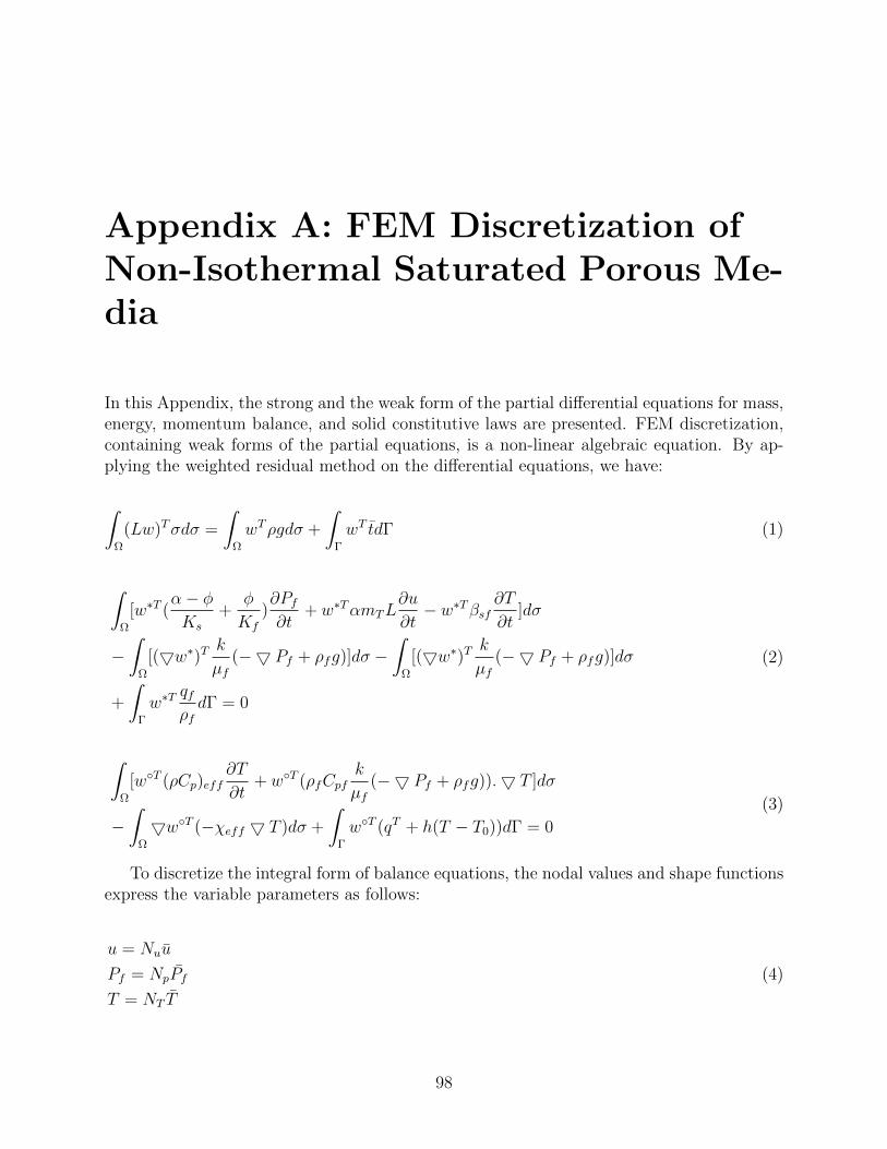
Appendix A: FEM Discretization ofNon-Isothermal Saturated Porous Me-dia

In this Appendix, the strong and the weak form of the partial differential equations for mass,energy, momentum balance, and solid constitutive laws are presented. FEM discretization,containing weak forms of the partial equations, is a non-linear algebraic equation. By ap-plying the weighted residual method on the differential equations, we have:

∫Ω

(Lw)Tσdσ =

∫Ω

wTρgdσ +

∫Γ

wT tdΓ (1)

∫Ω

[w∗T (α− φKs

+φ

Kf

)∂Pf∂t

+ w∗TαmTL∂u

∂t− w∗Tβsf

∂T

∂t]dσ

−∫

Ω

[(5w∗)T kµf

(−5 Pf + ρfg)]dσ −∫

Ω

[(5w∗)T kµf

(−5 Pf + ρfg)]dσ

+

∫Γ

w∗TqfρfdΓ = 0

(2)

∫Ω

[wT (ρCp)eff∂T

∂t+ wT (ρfCpf

k

µf(−5 Pf + ρfg)).5 T ]dσ

−∫

Ω

5wT (−χeff 5 T )dσ +

∫Γ

wT (qT + h(T − T0))dΓ = 0

(3)

To discretize the integral form of balance equations, the nodal values and shape functionsexpress the variable parameters as follows:

u = Nuu

Pf = NpPf

T = NT T

(4)

98

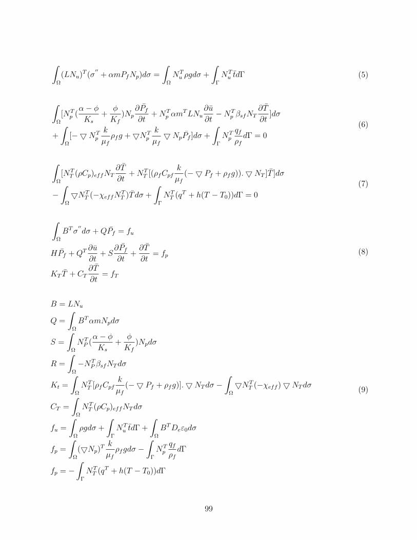
∫Ω

(LNu)T (σ

′′+ αmPfNp)dσ =

∫Ω

NTu ρgdσ +

∫Γ

NTu tdΓ (5)

∫Ω

[NTp (α− φKs

+φ

Kf

)Np∂Pf∂t

+NTp αm

TLNu∂u

∂t−NT

p βsfNT∂T

∂t]dσ

+

∫Ω

[−5NTp

k

µfρfg +5NT

p

k

µf5NpPf ]dσ +

∫Γ

NTp

qfρfdΓ = 0

(6)

∫Ω

[NTT (ρCp)effNT

∂T

∂t+NT

T [(ρfCpfk

µf(−5 Pf + ρfg)).5NT ]T ]dσ

−∫

Ω

5NTT (−χeffNT

T )T dσ +

∫Γ

NTT (qT + h(T − T0))dΓ = 0

(7)

∫Ω

BTσ′′dσ +QPf = fu

HPf +QT ∂u

∂t+ S

∂Pf∂t

+∂T

∂t= fp

KT T + CT∂T

∂t= fT

(8)

B = LNu

Q =

∫Ω

BTαmNpdσ

S =

∫Ω

NTP (α− φKs

+φ

Kf

)Npdσ

R =

∫Ω

−NTP βsfNTdσ

Kt =

∫Ω

NTT [ρfCpf

k

µf(−5 Pf + ρfg)].5NTdσ −

∫Ω

5NTT (−χeff )5NTdσ

CT =

∫Ω

NTT (ρCp)effNTdσ

fu =

∫Ω

ρgdσ +

∫Γ

NTu tdΓ +

∫Ω

BTDeε0dσ

fp =

∫Ω

(5Np)T k

µfρfgdσ −

∫Γ

NTp

qfρfdΓ

fp = −∫

Γ

NTT (qT + h(T − T0))dΓ

(9)

99

By applying the constitutive laws for an isotropic linear elastic medium, wee will have:

∫Ω

BTσ′′dσ =

∫Ω

BTDe(ε− ε0 − εT )dσ = −Keu+KteT −∫

Ω

BTDeε0dσ

Ke =

∫Ω

BTDeBdσ

Kte =

∫Ω

BTDemβs3NTdσ

(10)

The non-linear behavior of the solid phase can be established as:

∂P (u)

∂u= KT =

∫Ω

BTDTBdσ

∂P (u)

∂T= KtT = −

∫Ω

BTDemβs3NTdσ

(11)

Based on the above calculations, the governing equations can be written as:0 0 0

0 H 0

0 0 Kt

×

u

Pf

T

+

KT −Q KtT

QT S R

0 0 Ct

×

∂u

∂t

∂Pf∂t

∂T

∂t

=

∂fu∂t

fp

ft

(12)

To solve the dynamic problem, the central difference in time is applied to the abovegeneral equations:

KT −Q KtT

QT S − (1− θ)∆tH R

0 0 Ct − (1− θ)∆tKt

×un+1

Pfn+1

Tn+1

=

KT −Q KtT

QT S + θ∆tH R

0 0 Ct + θ∆tKt

×un

Pfn

Tn

+ ∆t

∂fu∂t

fp

ft

(13)

100

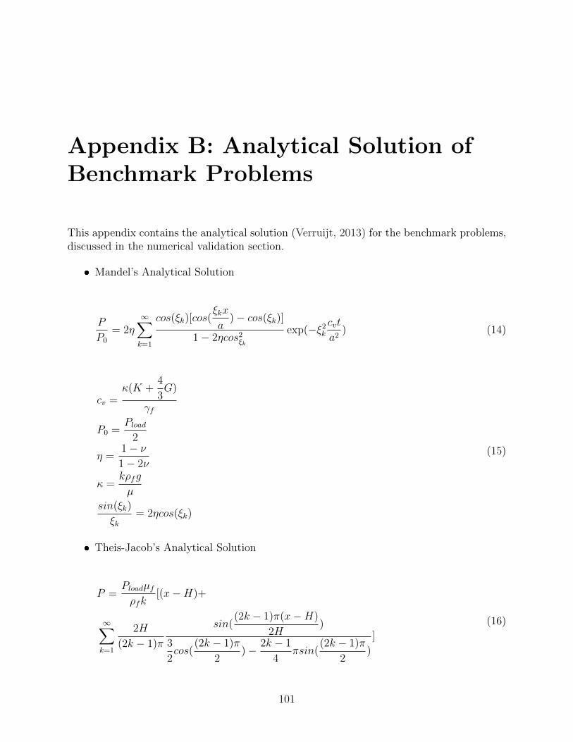
Appendix B: Analytical Solution ofBenchmark Problems

This appendix contains the analytical solution (Verruijt, 2013) for the benchmark problems,discussed in the numerical validation section.

Mandel’s Analytical Solution

P

P0

= 2η∞∑k=1

cos(ξk)[cos(ξkx

a)− cos(ξk)]

1− 2ηcos2ξk

exp(−ξ2k

cvt

a2) (14)

cv =κ(K +

4

3G)

γf

P0 =Pload

2

η =1− ν1− 2ν

κ =kρfg

µ

sin(ξk)

ξk= 2ηcos(ξk)

(15)

Theis-Jacob’s Analytical Solution

P =Ploadµfρfk

[(x−H)+

∞∑k=1

2H

(2k − 1)π

sin((2k − 1)π(x−H)

2H)

3

2cos(

(2k − 1)π

2)− 2k − 1

4πsin(

(2k − 1)π

2)

]

(16)

101

Verruijt, A. “Theory and problems of poroelasticity” Delft University of Technology, TheNetherlands (2013).

102

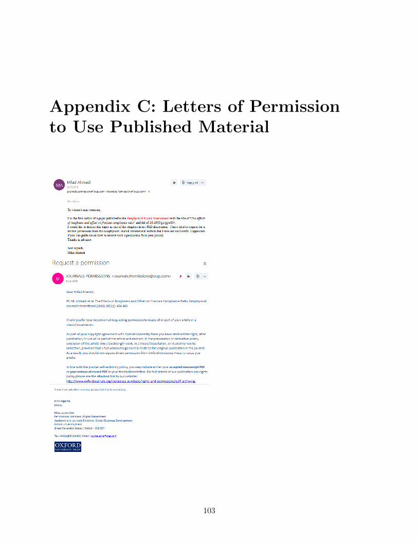
Appendix C: Letters of Permissionto Use Published Material

103

104

Vita

Milad Ahmadi was born in Tehran, Iran in 1986. He joined Craft and Hawkins Department

of Petroleum Engineering geomechanics research group at LSU as a Ph.D. student in Spring

2012 where he started his research under the supervision of Dr. Arash Dahi-Taleghani.

He holds a B. S. in Chemical Engineering and a M. S. degree in Petroleum Engineering

at University of Tehran. He is currently a member of Society of Petroleum Engineers (SPE),

American Rock Mechanics Association chapter LSU (ARMA), and American Petroleum

Professionals of Iranian Heritage (APPIH).

Milad Ahmadi is expected to receive his Doctor of Philosophy degree at the 2016 Summer

Commencement. He may be reached at milad.amd7@gmail.com in future.

105