A TRACE FINITE ELEMENT METHOD FOR A CLASS OFCOUPLED BULK-INTERFACE TRANSPORT PROBLEMS ∗

SVEN GROSS† , MAXIM A. OLSHANSKII‡ , AND ARNOLD REUSKEN§

Abstract. In this paper we study a system of advection-diffusion equations in a bulk domaincoupled to an advection-diffusion equation on an embedded surface. Such systems of coupled partialdifferential equations arise in, for example, the modeling of transport and diffusion of surfactants intwo-phase flows. The model considered here accounts for adsorption-desorption of the surfactants ata sharp interface between two fluids and their transport and diffusion in both fluid phases and alongthe interface. The paper gives a well-posedness analysis for the system of bulk-surface equationsand introduces a finite element method for its numerical solution. The finite element method isunfitted, i.e., the mesh is not aligned to the interface. The method is based on taking traces of astandard finite element space both on the bulk domains and the embedded surface. The numericalapproach allows an implicit definition of the surface as the zero level of a level-set function. Optimalorder error estimates are proved for the finite element method both in the bulk-surface energy normand the L2-norm. The analysis is not restricted to linear finite elements and a piecewise planarreconstruction of the surface, but also covers the discretization with higher order elements and ahigher order surface reconstruction.

1. Introduction. Coupled bulk-surface or bulk-interface partial differentialequations arise in many applications, e.g., in multiphase fluid dynamics [21] and bio-logical applications [2]. In this paper, we consider a coupled bulk-interface advection-diffusion problem. The problem arises in models describing the behavior of solublesurface active agents (surfactants) that are adsorbed at liquid-liquid interfaces. For adiscussion of physical phenomena related to soluble surfactants in two-phase incom-pressible flows we refer to the literature, e.g., [21, 30, 7, 32].

Systems of partial differential equations that couple bulk domain effects withinterface (or surface) effects pose challenges both for the mathematical analysis ofequations and the development and error analysis of numerical methods. These chal-lenges grow if phenomena occur at different physical scales, the coupling is nonlinearor the interface is evolving in time. To our knowledge, the analysis of numericalmethods for coupled bulk-surface (convection-)diffusion has been addressed in theliterature only very recently. In fact, problems related to the one studied in this pa-per have been considered only in [4, 15]. In these references finite element methodsfor coupled bulk-surface partial differential equations are proposed and analyzed. In[4, 15] a stationary diffusion problem on a bulk domain is linearly coupled with a sta-tionary diffusion equation on the boundary of this domain. A key difference betweenthe methods in [4] and [15] is that in the latter boundary fitted finite elements areused, whereas in the former unfitted finite elements are applied. Both papers includeerror analyses of these methods. In the recent paper [5] a similar coupled surface-bulksystem is treated with a different approach, based on the immersed boundary method.In that paper an evolving surface is considered, but only spatially two-dimensionalproblems are treated and no theoretical error analysis is given.

In the present paper, as in [4, 15] we restrict to stationary problems and a linear

∗Partially supported by NSF through the Division of Mathematical Sciences grant 1315993.†Institut fur Geometrie und Praktische Mathematik, RWTH-Aachen University, D-52056 Aachen,

Germany (gross@igpm.rwth-aachen.de)‡Department of Mathematics, University of Houston, Houston, Texas 77204-3008 (mol-

shan@math.uh.edu).§Institut fur Geometrie und Praktische Mathematik, RWTH-Aachen University, D-52056 Aachen,

Germany (reusken@igpm.rwth-aachen.de).

1

arX

iv:1

406.

7694

v3 [

mat

h.N

A]

8 D

ec 2

014

coupling. The results obtained are a starting point for research on other classes ofproblems, e.g., with an evolving interface, cf. the discussion in section 10. The twomain new contributions of this paper are the following. Firstly, the class of problemsconsidered is significantly different from the one treated in [4, 15]. We study a problemin which elliptic partial differential equations in two bulk subdomains are coupled to apartial differential equation on a sharp interface which separates the two subdomains.In the previous work only a coupling of an elliptic partial differential in one bulkdomain with a partial differential equation on the boundary of this bulk domain istreated. Furthermore, the partial differential equations considered in this paper arenot pure diffusion equations, but convection-diffusion equations. The latter modelthe transport by advection and diffusion of surfactants. We will briefly address somebasic modeling aspects, e.g. related to adsorption (Henry and Langmuir laws), ofthese coupled equations. The first main new result is the well-posedness of a weakformulation of this coupled system. We introduce suitable function spaces and anappropriate weak formulation of the problem. We derive a Poincare type inequalityin a bulk-interface product Sobolev space and show an inf-sup stability result for thebilinear form of the weak formulation. This then leads to the well-posedness result.The second main new contribution is the error analysis of a finite element method.We consider an unfitted finite element method, which is very similar to the methodpresented in [4]. In the method treated in this paper we do not apply the stabilizationtechnique used in [4]. An unfitted approach is particularly attractive for problems withan evolving interface, which will be studied in a follow-up paper. Both interface andbulk finite element spaces are trace spaces of globally defined continuous finite elementfunctions with respect to a regular simplicial triangulation of the whole domain. Forbulk problems, such finite element techniques have been extensively studied in theliterature on cut finite element methods or XFEM, cf. e.g. [22, 23, 3]. For PDEsposed on surfaces, the trace finite element method was introduced and studied in[26, 28, 24, 11]. In the method that we propose, the smooth interface is approximatedby a piecewise smooth one, characterized by the zero level set of a finite element levelset function. This introduces a geometric error in the method. The approach allowsmeshes that do not fit to this (approximate) interface and admits implicitly definedinterfaces. The finite element formulation is shown to be well-posed. We present anerror analysis that is general in the sense that finite element polynomials of arbitrarydegree are allowed (in [4] only linear finite elements are treated) and that the accuracyof the interface approximation can be varied. The error analysis is rather technicaland we aimed at a clear exposition by subdividing the analysis into several steps: theconstruction of a bijective mapping between the continuous bulk domains and theirnumerical approximations, the definition and analysis of extensions of functions offthe interface and outside the bulk domains, and the analysis of consistency terms in anapproximate Galerkin orthogonality property. This leads to an optimal order boundfor the discretization error in the energy norm of the product space. Finally, by usinga suitable adjoint problem, we derive an optimal order error bound in the L2 productnorm. Results of numerical experiments are included that illustrate the convergencebehavior of the finite element method. A point that we do not address in this paper isthe stabilization of the discretization method with respect to the conditioning of thestiffness matrix. From the literature it is known that the trace finite element approachresults in a poor conditioning of the stiffness matrix. The technique presented in [3, 4]can be used (for linear finite elements) to obtain a stiffness matrix with conditioningproperties similar to those of a standard finite element method. We think that this

2

technique is applicable also to the method presented in this paper, but decided notto include it, since the additional stabilization terms would lead to a further increaseof technicalities in the analysis. Finally we mention the recent related paper [8], inwhich unfitted finite element techniques, similar to the one used in this paper, areapplied to surface partial differential equations (without coupling to bulk domains).

2. Mathematical model. In this section we explain the physical backgroundof the coupled bulk-interface model that we treat in this paper. Consider a two-phaseincompressible flow system in which two fluids occupy subdomains Ωi(t), i = 1, 2, ofa given domain Ω ⊂ R3. The corresponding velocity field of the fluids is denoted byw(x, t), x ∈ Ω, t ∈ [0, t1]. For convenience, we assume that Ω1(t) is simply connectedand strictly contained in Ω (e.g., a rising droplet) for all t ∈ [0, t1]. The outwardpointing normal from Ω1 into Ω2 is denoted by n. The sharp interface between thetwo fluids is denoted by Γ(t). Below we write Γ instead of Γ(t). It is assumed that thefluids are immiscible and that there are no phase changes. Consequently, the normalcomponents of the fluid velocity are continuous at the interface and the interface itselfis advected with the flow, i.e., VΓ = w ·n holds, where VΓ denotes the normal velocityof the interface. The standard model for the fluid dynamics in such a system consistsof the Navier-Stokes equations, combined with suitable coupling conditions at theinterface. In the rest of this paper, we assume that the velocity field has smoothnessw(·, t) ∈ [H1,∞(Ω) ∩ H1(Γ)]3 and that w is given, i.e., we do not consider a two-way coupling between surfactant transport and fluid dynamics. The fluid is assumedincompressible:

div w = 0 in Ω. (2.1)

Consider a surfactant that is soluble in both phases and can be adsorbed anddesorbed at the interface. The surfactant volume concentration (i.e., the one in thebulk phases) is denoted by u, ui = u|Ωi , i = 1, 2. The surfactant area concentra-tion on Γ is denoted by v. Change of the surfactant concentration happens due toconvection by the velocity field w, diffusive fluxes in Ωi, a diffusive flux on Γ andfluxes coming from adsorption and desorption. The net flux (per surface area) due toadsorption/desorption between Ωi and Γ is denoted by ji,a − ji,d. The total net flux

is ja − jd =∑2i=1(ji,a − ji,d). Mass conservation in a control volume (transported by

the flow field) that is strictly contained in Ωi results in the bulk convection-diffusionequation

∂u

∂t+ w · ∇u−Di∆u = 0 in Ωi = Ωi(t), i = 1, 2. (2.2)

Here Di > 0 denotes the bulk diffusion coefficient, which is assumed to be constantin Ωi. Mass conservation in a control area (transported by the flow field) that iscompletely contained in Γ results in the surface convection-diffusion equation (cf. [21]):

v + (divΓ w)v −DΓ∆Γv = ja − jd on Γ = Γ(t), (2.3)

where v = ∂v∂t + w · ∇v denotes the material derivative and ∆Γ, divΓ the Laplace-

Beltrami and surface divergence operators, respectively. The interface diffusion coef-ficient DΓ > 0 is assumed to be a constant.

We assume that transport of surfactant between the two phases can only occurvia adsorption/desorption. Due to VΓ = w · n, the mass flux through Γ equals thediffusive mass flux. Hence, mass conservation in a control volume (transported by

3

the flow field) that lies in Ωi and with part of its boundary on Γ results in the massbalance equations

(−1)iDin · ∇ui = ji,a − ji,d, i = 1, 2. (2.4)

The sign factor (−1)i accounts for the fact that the normal n is outward pointingfrom Ω1 into Ω2. Summing these relations over i = 1, 2, yields

ja − jd = −[Dn · ∇u]Γ,

where [w]Γ = (w1)|Γ − (w2)|Γ denotes the jump of w across Γ.To close the system of equations, we need constitutive equations for modeling the

adsorption/desorption. A standard model, cf. [30], is as follows:

ji,a − ji,d = ki,agi(v)ui − ki,dfi(v), on Γ, (2.5)

with ki,a, ki,d positive adsorption and desorption coefficients that describe the kinetics.We consider two fluids having similar adsorption/desorption behavior in the sense thatthe coefficients ki,a, ki,d may depend on i, but gi(v) = g(v), fi(v) = f(v) for i = 1, 2.Basic choices for g, f are the following:

g(v) = 1, f(v) = v (Henry) (2.6)

g(v) = 1− v

v∞, f(v) = v (Langmuir), (2.7)

where v∞ is a constant that quantifies the maximal concentration on Γ. Furtheroptions are given in [30]. Note that in the Langmuir case we have a nonlinearity dueto the term vui. Combining (2.2), (2.3), (2.4) and (2.5) gives a closed model. For themathematical analysis it is convenient to reformulate these equations in dimensionlessvariables. Let L, W be appropriately defined length and velocity scales and T = L/Wthe corresponding time scale. Furthermore, U and V are typical reference volume andarea concentrations. The equations above can be reformulated in the dimensionlessvariables x = x/L, t = t/T , ui = ui/U , v = v/V , w = w/W . This results in thefollowing system of coupled bulk-interface convection-diffusion equations, where weuse the notation x, t, ui, v,w also for the transformed variables:

∂u

∂t+ w · ∇u− νi∆u = 0 in Ωi(t), i = 1, 2,

v + (divΓ w)v − νΓ∆Γv = −K[νn · ∇u]Γ on Γ(t),

(−1)iνin · ∇ui = ki,ag(v)ui − ki,dv on Γ(t), i = 1, 2,

with νi =Di

LW, νΓ =

DΓ

LW, K =

LU

V, ki,a =

T

Lki,a, ki,d =

T

Kki,d,

(2.8)

and g(v) = 1 (Henry) or g(v) = 1− Vv∞v (Langmuir). This model has to be comple-

mented by suitable initial conditions for u, v and boundary conditions on ∂Ω for u.The resulting model is often used in the literature for describing surfactant behavior,e.g. [14, 32, 12, 5]. The coefficients ki,a, ki,d are the dimensionless adsorption anddesorption coefficients.

Remark 1. Sometimes, in the literature the Robin type interface conditions(−1)iνin·∇ui = ki,ag(v)ui−ki,dv in (2.8) are replaced by (simpler) Dirichlet type con-

ditions. In case of “instantaneous” adsorption and desorption one may assume ki,a 4

νi, ki,d νi and the Robin interface conditions are approximated by ki,ag(v)ui =

ki,dv, i = 1, 2.

From a mathematical point of view, the problem (2.8) is challenging, becauseconvection-diffusion equations in the moving bulk phase Ωi(t) are coupled with aconvection-diffusion equation on the moving interface Γ(t). As far as we know, forthis model there are no rigorous results on well-posedness known in the literature, cf.also Remark 2 below.

3. Simplified model. As a first step in the analysis of the problem (2.8) weconsider a simplified model. We restrict to g(v) = v (Henry’s law), consider the sta-tionary case and make some (reasonable) assumptions on the range of the adsorptionand desorption parameters ki,a, ki,d. In the remainder we assume that Ωi and Γ donot depend on t (e.g., an equilibrium motion of a rising droplet in a suitable frameof reference). Since the interface is passively advected by the velocity field w, thisassumption leads to the constraint

w · n = 0 on Γ. (3.1)

We also assume divΓ w = 0 so that the term (divΓ w)v in the surface convection-diffusion equation vanishes. Furthermore, for the spatial part of the material deriva-tive v we have w · ∇v = w · ∇Γv. We let the normal part of w to vanish on exteriorboundary:

w · nΩ = 0 on ∂Ω, (3.2)

where nΩ denotes the outward pointing normal on ∂Ω. From (3.2) it follows thatthere is no convective mass flux across ∂Ω. We also assume no diffusive mass fluxacross ∂Ω, i.e. the homogeneous Neumann boundary condition nΩ · ∇u2 = 0 on ∂Ω.Restricting the model (2.8) to an equilibrium state, we obtain the following stationaryproblem:

−νi∆ui + w · ∇ui = fi in Ωi, i = 1, 2,

−νΓ∆Γv + w · ∇Γv +K[νn · ∇u]Γ = g on Γ,

(−1)iνin · ∇ui = ki,aui − ki,dv on Γ, i = 1, 2,

nΩ · ∇u2 = 0 on ∂Ω.

(3.3)

In this model, we allow source terms g ∈ L2(Γ) and fi ∈ L2(Ωi). Using partialintegration over Ωi, i = 1, 2, and over Γ, one checks that these source terms have tosatisfy the consistency condition

K( ∫

Ω1

f1 dx +

∫Ω2

f2 dx)

+

∫Γ

g ds = 0. (3.4)

A simplified version of this model, namely with only one bulk domain Ω1 and withw = 0 (only diffusion) has recently been analyzed in [15].

From physics it is known that for surfactants almost always the desorption ratesare (much) smaller than the adsorption rates. Therefore, it is reasonable to assumeki,d ≤ cki,a with a “small” constant c. To simplify the presentation, we assume

ki,d ≤ k1,a + k2,a for i = 1, 2. For the adsorption rates ki,a we exclude the singular-

perturbed cases ki,a ↓ 0 and ki,a → ∞. Summarizing, we consider the parameterranges

ki,a ∈ [kmin, kmax], ki,d ∈ [0, k1,a + k2,a], (3.5)

5

with fixed generic constants kmin > 0, kmax. Note that unlike in previous studies weallow ki,d = 0 (i.e., only adsorption). Finally, due to the restriction on the adsorption

parameter ki,a given in (3.5) we can use the following transformation to reduce thenumber of parameters of the model (3.3):

ui := ki,aui, v := (k1,a + k2,a)v,

νi := k−1i,a νi, νΓ := νΓ/(k1,a + k2,a),

wi := k−1i,aw in Ωi, w := w/(k1,a + k2,a) on Γ.

(3.6)

Note that after this transformation w will in general be discontinuous across Γ. Ineach subdomain and on Γ, however, w is regular: w|Ωi = wi ∈ H1,∞(Ωi)

3, i = 1, 2,and w|Γ ∈ H1(Γ)3. For simplicity we omit the tilde notation in the transformedvariables. This then results in the following model, which we study in the remainderof the paper:

−νi∆ui + w · ∇ui = fi in Ωi, i = 1, 2,

−νΓ∆Γv + w · ∇Γv +K[νn · ∇u]Γ = g on Γ,

(−1)iνin · ∇ui = ui − qiv on Γ, i = 1, 2,

nΩ · ∇u2 = 0 on ∂Ω,

with qi :=ki,d

k1,a + k2,a

∈ [0, 1].

(3.7)

The data fi and g are assumed to satisfy the consistency condition (3.4). Recall thatK = LU

V > 0, cf. (2.8), is a fixed (scaling) constant.

4. Analysis of well-posedness. In this section we derive a suitable weak for-mulation of the problem (3.7) and prove well-posedness of this weak formulation.Concerning the smoothness of the interface, we assume that Γ is a C1 manifold. Thisassumption also suffices for the analysis in section 5.

We first introduce some notations. For u ∈ H1(Ω1∪Ω2) we also write u = (u1, u2)with ui = u|Ωi ∈ H1(Ωi). Furthermore:

(f, g)ω :=

∫ω

fg dx, ‖f‖2ω := (f, f)ω, where ω is any of Ω,Ωi,Γ,

(∇u,∇w)Ω1∪Ω2 :=∑i=1,2

∫Ωi

∇ui · ∇wi dx, u, w ∈ H1(Ω1 ∪ Ω2),

‖u‖21,Ω1∪Ω2:= ‖u1‖2H1(Ω1) + ‖u2‖2H1(Ω2) = ‖u‖2Ω + ‖∇u‖2Ω1∪Ω2

.

We need a suitable gauge condition. In the original dimensional variables a naturalcondition is conservation of total mass, i.e. (u1, 1)Ω1

+ (u2, 1)Ω2+ (v, 1)Γ = m0,

with m0 > 0 the initial total mass. Due to the transformation of variables andwith an additional constant shift this condition is transformed to Kk−1

1,a(u1, 1)Ω1 +

Kk−12,a(u2, 1)Ω1

+ (k1,a + k2,a)−1(v, 1)Γ = 0 for the variables used in (3.7). Hence, weobtain the natural gauge condition

K(1 + r)(u1, 1)Ω1+K(1 +

1

r)(u2, 1)Ω2 + (v, 1)Γ = 0, r :=

k2,a

k1,a

. (4.1)

6

Define the product spaces

V = H1(Ω1 ∪ Ω2)×H1(Γ), ‖(u, v)‖V :=(‖u‖21,Ω1∪Ω2

+ ‖v‖21,Γ) 1

2 ,

V = (u, v) ∈ V | (u, v) satisfies (4.1) .

To obtain the weak formulation, we multiply the bulk and surface equation in(3.7) by test functions from V, integrate by parts and use interface and boundary

conditions. The resulting weak formulation reads: Find (u, v) ∈ V such that for all(η, ζ) ∈ V:

a((u, v); (η, ζ)) = (f1, η1)Ω1+ (f2, η2)Ω2

+ (g, ζ)Γ, (4.2)

a((u, v); (η, ζ)) := (ν∇u,∇η)Ω1∪Ω2+ (w · ∇u, η)Ω1∪Ω2

+ νΓ(∇Γv,∇Γζ)Γ

+ (w · ∇Γv, ζ)Γ +

2∑i=1

(ui − qiv, ηi −Kζ)Γ.

For the further analysis, we note that both w-dependent parts of the bilinear form in(4.2) are skew-symmetric:

(w · ∇ui, ηi)Ωi = −(w · ∇ηi, ui)Ωi , i = 1, 2, (w · ∇Γv, ζ)Γ = −(w · ∇Γζ, v)Γ. (4.3)

To verify the first equality in (4.3), one integrates by parts over each subdomain Ωi:

(w · ∇u1, η1)Ω1= −(w · ∇η1, u1)Ω1

− ((div w)η1, u1)Ω1+ ((n ·w)η1, u1)Γ,

(w · ∇u2, η2)Ω2= −(w · ∇η2, u2)Ω2

− ((div w)η2, u2)Ω2− ((n ·w)η2, u2)Γ

+ ((nΩ ·w)η2, u2)∂Ω2∩∂Ω.

All terms with div w, n ·w or nΩ ·w vanish due to (2.1), (3.1) and (3.2).The variational formulation in (4.2) is the basis for the finite element method

introduced in section 6. For the analysis of well-posedness, it is convenient to introducean equivalent formulation where the test space V is replaced by a smaller one, in whicha suitable gauge condition is used. For this we define, for α = (α1, α2) with αi ≥ 0,the space

Vα := (u, v) ∈ V | α1(u1, 1)Ω1+ α2(u2, 1)Ω2

+ (v, 1)Γ = 0 .

Note that V = Vα for α = (K(1 + r),K(1 + 1r )), cf. (4.1). The data f1, f2, g, satisfy

the consistency property (3.4). From this and (4.3) it follows that if a pair of trial andtest functions ((u, v); (η, ζ)) satisfies (4.2) then ((u, v); (η, ζ) + γ(K, 1)) also satisfies(4.2) for arbitrary γ ∈ R. Now let an arbitrary α = (α1, α2) be given. For every(η, ζ) ∈ V there exists γ ∈ R and (η, ζ) ∈ Vα such that (η, ζ) = (η, ζ)+γ(K, 1) holds.

From this it follows that (4.2) is equivalent to the following problem: Find (u, v) ∈ Vsuch that for all (η, ζ) ∈ Vα:

a((u, v); (η, ζ)) = (f1, η1)Ω1 + (f2, η2)Ω2 + (g, ζ)Γ. (4.4)

For this weak formulation we shall analyze well-posedness.For H1(Ωi) and H1(Γ) the following Poincare-Friedrich’s inequalities hold:

‖ui‖2Ωi ≤ c(‖∇ui‖2Ωi + (ui, 1)2

Ωi) for all ui ∈ H1(Ωi), (4.5)

‖ui‖2Ωi ≤ c(‖∇ui‖2Ωi + ‖ui‖2Γ) for all ui ∈ H1(Ωi), (4.6)

‖v‖2Γ ≤ c(‖∇Γv‖2Γ + (v, 1)2Γ) for all v ∈ H1(Γ). (4.7)

7

For the analysis of stability of the weak formulation we need the following Poincaretype inequality in the space V.

Lemma 4.1. Let ri, σi ∈ [0,∞), i = 1, 2. There exists CP (r1, r2, σ1, σ2) > 0 suchthat for all (u, v) ∈ V, the following inequality holds:

‖(u, v)‖V ≤ CP(‖∇u‖Ω1∪Ω2

+ ‖∇Γv‖Γ

+ |r1(u1, 1)Ω1 + r2(u2, 1)Ω2 + (v, 1)Γ|+2∑i=1

|(ui − σiv, 1)Γ|).(4.8)

Proof. The result follows from the Petree-Tartar Lemma (cf., [16]). For conve-nience, we recall the lemma: Let X,Y, Z be Banach spaces, A ∈ L(X,Y ) injective,T ∈ L(X,Z) compact and assume

‖x‖X ≤ c(‖Ax‖Y + ‖Tx‖Z

)for all x ∈ X. (4.9)

Then there exists a constant c such that

‖x‖X ≤ c‖Ax‖Y for all x ∈ X (4.10)

holds. We take X = H1(Ω1)×H1(Ω2)×H1(Γ) with the norm

‖(u1, u2, v)‖X = (‖u1‖21,Ω1+ ‖u2‖21,Ω2

+ ‖v‖21,Γ)12 .

Furthermore, Y = L2(Ω1)3 × L2(Ω2)3 × L2(Γ)3 × R3 with the product norm andZ = L2(Ω1) × L2(Ω2) × L2(Γ) with the product norm. We introduce the bilinearforms

l0(u1, u2, v) := r1(u1, 1)Ω1+ r2(u2, 1)Ω2

+ (v, 1)Γ,

l1(u1, u2, v) = (u1 − σ1v, 1)Γ,

l2(u1, u2, v) = (u2 − σ2v, 1)Γ,

and define the linear operators

A(u1, u2, v) = (∇u1,∇u2,∇Γv, l0(u1, u2, v), l1(u1, u2, v), l2(u1, u2, v)),

T (u1, u2, v) = (u1, u2, v).

Then we have A ∈ L(X,Y ). Consider A(u1, u2, v) = 0. The first 9 equations yieldu1 =constant, u2 =constant, v =constant, and substitution of this in the last threeequations yields that these constants must be zero. Hence, A is injective. The oper-ator T ∈ L(X,Z) is compact. This follows from the compactness of the embeddingsH1(Ωi) → L2(Ω), H1(Γ) → L2(Γ). It is easy to check that the inequality (4.9) is sat-

isfied. The Petree-Tartar Lemma implies (‖u‖21,Ω1∪Ω2+ ‖v‖21,Γ)

12 ≤ c‖A(u1, u2, v)‖Y

and thus the estimate (4.8) holds.

The next theorem states an inf-sup stability estimate for the bilinear form in(4.4).

Theorem 4.2. There exists Cst > 0 such that for all q1, q2 ∈ [0, 1] and with asuitable α = α(q1, q2) the following holds:

inf(u,v)∈V

sup(η,ζ)∈Vα

a((u, v); (η, ζ))

‖(u, v)‖V‖(η, ζ)‖V≥ Cst. (4.11)

8

Proof. Let (u, v) ∈ V be given. Note that (u, v) satisfies the gauge condition(4.1). We first treat the case 0 ≤ q2 ≤ q1 ≤ 1. We consider three cases depending onvalues of these parameters.

We first consider q1, q2 ∈ [0, ε], with ε > 0 specified below. We take η1 = βu1,η2 = βu2, with β > 0, and ζ = v. The value of β is chosen further on. This yields

a((u, v); (η, ζ)) = ν1β‖∇u1‖2Ω1+ ν2β‖∇u2‖2Ω2

+ νΓ‖∇Γv‖2Γ + β‖u1‖2Γ + β‖u2‖2Γ

−2∑i=1

(qiβ +K)(ui, v)Γ +K(q1 + q2)‖v‖2Γ

≥ β‖ν∇u‖2Ω1∪Ω2+

1

2β‖u1‖2Γ +

1

2β‖u2‖2Γ + νΓ‖∇Γv‖2Γ − (εβ

12 +Kβ−

12 )2‖v‖2Γ

≥ cFβ‖u‖21,Ω1∪Ω2+ νΓ‖∇Γv‖2Γ − (εβ

12 +Kβ−

12 )2‖v‖2Γ,

where in the last inequality we used (4.6). The constant cF > 0 depends only on theFriedrich’s constant from (4.6) and the viscosity ν. From the gauge condition we get

(v, 1)2 ≤ 2K2((1 + r)2(u1, 1)2

Ω1+ (1 +

1

r)2(u2, 1)2

Ω2

)≤ c(‖u1‖2Ω1

+ ‖u2‖2Ω2

)= c‖u‖2Ω.

Using this and the Poincare’s inequality in (4.7) we obtain

a((u, v); (η, ζ))

≥ cFβ‖u‖21,Ω1∪Ω2+ νΓ(‖∇Γv‖2Γ + (v, 1)2

)− c‖u‖2Ω − (εβ

12 +Kβ−

12 )2‖v‖2Γ

≥ cFβ‖u‖21,Ω1∪Ω2+ cF ‖v‖21,Γ − c‖u‖2Ω − (εβ

12 +Kβ−

12 )2‖v‖2Γ.

The constant c depends only on νΓ, r,K. The constant cF > 0 depends only on aPoincare’s constant and νΓ. We take β sufficiently large (depending only on cF , c andK) and ε > 0 sufficiently small such that the third term can be adsorbed in the firstone and the last term can be adsorbed in the second one. Thus we get

a((u, v); (η, ζ)) ≥ c‖(u, v)‖2V ≥ c‖(u, v)‖V‖(η, ζ)‖V,

which completes the proof of (4.11) for the first case. Now ε > 0 is fixed.In the second case we take q1 ≥ ε, and q2 ∈ [0, δ], with a δ ∈ (0, ε] that will be

specified below. We take η1 = u1, η2 = 0, ζ = K−1q1v. Using the gauge conditionand (4.8) with u2 = 0, σ2 = 0, r1 = K(1 + r), σ1 = q1, we get

a((u, v); (η, ζ)) = ν1‖∇u1‖2Ω1+q1νΓ

K‖∇Γv‖2Γ + ‖u1 − q1v‖2Γ − q1(u2, v)Γ + q2q1‖v‖2Γ

≥ ν1‖∇u1‖2Ω1+ενΓ

K‖∇Γv‖2Γ + ‖u1 − q1v‖2Γ

+ |K(1 + r)(u1, 1)Ω1+ (v, 1)Γ|2 −K2(1 +

1

r)2(u2, 1)2

Ω2− q1(u2, v)Γ

≥ cF(‖u1‖21,Ω1

+ ‖v‖21,Γ)− c‖u2‖2Ω2

− ‖u2‖Γ‖v‖Γ

≥ 1

2cF(‖u1‖21,Ω1

+ ‖v‖21,Γ)− c(‖u2‖2Ω2

+ ‖u2‖2Γ). (4.12)

The constant cF > 0 depends on Poincare’s constant and on ε. We now take η1 =0, η2 = βu2, with β > 0 and ζ = 0. This yields, cf. (4.6),

a((u, v); (η, ζ)) = ν2β‖∇u2‖2Ω1+ β‖u2‖2Γ − βq2(u2, v)Γ ≥ cβ‖u2‖21,Ω2

− 1

2βδ2‖v‖2Γ.

9

Combining this with (4.12) and taking β sufficiently large such that the last term in(4.12) can be adsorbed, we obtain for η1 = u1, η2 = βu2, ζ = K−1q1v:

a((u, v); (η, ζ)) ≥ 1

2cF(‖u1‖21,Ω1

+ ‖v‖21,Γ)

+ cβ‖u2‖21,Ω2− 1

2βδ2‖v‖2Γ.

Now we take δ > 0 sufficiently small such that the last term can be adsorbed by thesecond one. Hence,

a((u, v); (η, ζ)) ≥ c‖(u, v)‖2V ≥ c‖(u, v)‖V‖(η, ζ)‖V,

which completes the proof of the inf-sup property for the second case. Now δ > 0 isfixed.

We consider the last case, namely q1 ≥ δ and q2 ≥ δ. Take η1 = u1, η2 = q1q2u2,

ζ = K−1q1v. We then get

a((u, v); (η, ζ)) = ν1‖∇u1‖2Ω1+ ν2

q1

q2‖∇u2‖2Ω2

+νΓq1

K‖∇Γv‖2Γ

+ ‖u1 − q1v‖2Γ +q1

q2‖u2 − q2v‖2Γ

≥ c(‖∇u‖2Ω1∪Ω2

+ ‖∇Γv‖2Γ +

2∑i=1

‖ui − qiv‖2Γ).

We use (4.8) with r1 = K(1 + r), r2 = K(1 + 1r ), with r from (4.1), and σi = qi. This

yields

a((u, v); (η, ζ)) ≥ c‖(u, v)‖2V ≥ c‖(u, v)‖V‖(η, ζ)‖V,

with a constant c > 0 that depends on δ, but is independent of (u, v).In all three cases, since (u, v) obeys the gauge condition (4.1), we get (η, ζ) ∈ Vα,

for suitable α = (α1, α2) with αi > 0.The case 0 ≤ q1 ≤ q2 ≤ 1 can be treated with almost exactly the same arguments.

Note that the α used in Theorem 4.2 may depend on qi. In the remainder, forgiven problem parameters qi ∈ [0, 1], i = 1, 2, we take α as in Theorem 4.2 and usethis α in the weak formulation (4.2). For the analysis of a dual problem, we also needthe stability of the adjoint bilinear form given in the next lemma.

Lemma 4.3. There exists Cst > 0 such that for all q1, q2 ∈ [0, 1] and with α asin Theorem 4.2 the following holds:

inf(η,ζ)∈Vα

sup(u,v)∈V

a((u, v); (η, ζ))

‖(u, v)‖V‖(η, ζ)‖V≥ Cst. (4.13)

Proof. Take (η, ζ) ∈ Vα, (η, ζ) 6= (0, 0). The arguments of the proof of Theo-

rem 4.2 show that for (η, ζ) ∈ Vα there exists (u, v) ∈ V such that a((u, v); (η, ζ)) ≥Cst‖(u, v)‖V‖(η, ζ)‖V holds, with the same constant as (4.11).

Finally, we give a result on continuity of the bilinear form.Lemma 4.4. There exists a constant c such that for all q1, q2 ∈ [0, 1] the following

holds:

a((u, v); (η, ζ)) ≤ c‖(u, v)‖V‖(η, ζ)‖V for all (u, v), (η, ζ) ∈ V.

10

Proof. The continuity estimate is a direct consequence of Cauchy-Schwarz in-equalities and boundedness of the trace operator.

We obtain the following well-posedness and regularity results.

Theorem 4.5. For any fi ∈ L2(Ωi), i = 1, 2, g ∈ L2(Γ) such that (3.4) holds,

there exists a unique solution (u, v) ∈ V of (4.2), which is also the unique solution to(4.4). This solution satisfies the a-priori estimate

‖(u, v)‖V ≤ C‖(f1, f2, g)‖V′ ≤ c(‖f1‖Ω1+ ‖f2‖Ω2

+ ‖g‖Γ), (4.14)

with constants C, c independent of fi, g and q1, q2 ∈ [0, 1]. If in addition Γ is a C2-manifold and Ω is convex or ∂Ω is C2 smooth, then ui ∈ H2(Ωi), for i = 1, 2, andv ∈ H2(Γ). Furthermore, the solution satisfies the second a-priori estimate

‖u1‖H2(Ω1) + ‖u2‖H2(Ω2) + ‖v‖H2(Γ) ≤ c(‖f1‖Ω1+ ‖f2‖Ω2

+ ‖g‖Γ). (4.15)

Proof. Existence, uniqueness and the first a-priori estimate follow from Theo-rem 4.2 and the Lemmas 4.3 and 4.4. To show the extra regularity of the solution, wenote that ui satisfies the weak formulation of the Poisson equation −νi∆ui = Fi :=fi −w · ∇ui in Ωi with a Robin boundary condition (−1)in · ∇ui − ui = Gi := −qiv.

Thanks to (4.14) we have Fi ∈ L2(Ωi), Gi ∈ H12 (∂Ωi) and ‖Fi‖Ωi + ‖Gi‖

H12 (∂Ωi)

≤c(‖f1‖Ω1 + ‖f2‖Ω2 + ‖g‖Γ). Theorem 2.4.2.6 from [19] implies ui ∈ H2(Ωi) and theestimate for ui in (4.15). On the interface Γ, v satisfies the weak formulation of theLaplace-Beltrami equation −νΓ∆Γv = GΓ := g−w·∇Γv−K[n·∇u]. Thanks to (4.14),the regularity result for ui in (4.15) and the smoothness of Γ, we have GΓ ∈ L2(Γ)and ‖GΓ‖Γ ≤ c(‖f1‖Ω1

+ ‖f2‖Ω2+ ‖g‖Γ). Now we apply the regularity result for

the Laplace-Beltrami equation on a closed C2-surface from Lemma 3.2 in [13]. Thisproves v ∈ H2(Γ) and the estimate on ‖v‖H2(Γ) in (4.15).

Remark 2. In [4, 15] a stationary diffusion problem on a bulk domain is linearlycoupled with a stationary diffusion equation on the boundary of this domain. Hencethere is only one bulk domain. Well-posedness of a suitable weak formulation of thisproblem is shown in [15, 1]. The analysis in [15] is significantly simpler than theone presented above. This is due to the fact that for the case of one bulk domainthe coupling term is simpler and one easily verifies that the corresponding bilinearform is elliptic. In our case, due to the coupling term

∑2i=1(ui − qiv, ηi − Kζ)Γ in

(4.2), the bilinear form is not elliptic and we have to derive an inf-sup estimate. Afurther complication, compared to the case of one bulk domain, is the Poincare typeinequality that we need, cf. Lemma 4.1.

5. Adjoint problem. Consider the following formal adjoint problem, with α asin Theorem 4.2. For given f ∈ L2(Ω) and g ∈ L2(Γ) find (u, v) ∈ Vα such that for

all (η, ζ) ∈ V:

a((η, ζ); (u, v)) = (f1, η1)Ω1 + (f2, η2)Ω2 + (g, ζ)Γ. (5.1)

Due to the results in Theorem 4.2 and Lemmas 4.3, 4.4, the problem (5.1) is well-posed.

11

Now we look for the corresponding strong formulation of this adjoint problem.We introduce an appropriate gauge condition for the right-hand side:

q1(f1, 1)Ω1 + q2(f2, 1)Ω2 + (g, 1)Γ = 0. (5.2)

For any (η1, η2, ζ) ∈ V there is a γ ∈ R such that (η1, η2, ζ) + γ(q1, q2, 1) ∈ Vholds. From the definition of the bilinear form it follows that a((q1, q2, 1); (u, v)) = 0holds. Hence, if the right-hand side satisfies condition (5.2), the formulation (5.1) isequivalent to: Find (u, v) ∈ Vα such that

a((η, ζ); (u, v)) = (f1, η1)Ω1+ (f2, η2)Ω2

+ (g, ζ)Γ for all (η, ζ) ∈ V.

Varying (η, ζ) we find the strong formulation of the dual problem to (3.7):

−νi∆ui −w · ∇ui = fi in Ωi, i = 1, 2,

−νΓ∆Γv −w · ∇Γv + [qνn · ∇u]Γ = g on Γ,

(−1)iνin · ∇ui = ui −Kv on Γ, i = 1, 2,

nΩ · ∇u2 = 0 on ∂Ω.

(5.3)

In the second equation q denotes a piecewise constant function with values q|Ωi := qi.Note that compared to the original primal problem (3.7) we now have −w instead ofw and that the roles of K and q are interchanged. With the same arguments as forthe primal problem, cf. Theorem 4.5, the following H2-regularity result for the dualproblem can be derived.

Theorem 5.1. For any fi ∈ L2(Ωi), i = 1, 2, g ∈ L2(Γ) such that (5.2) holds,there exists a unique weak solution (u, v) ∈ Vα of (5.3). If Γ is a C2-manifold and Ωis convex or ∂Ω is C2 smooth, then ui ∈ H2(Ωi), for i = 1, 2, and v ∈ H2(Γ) satisfythe a-priori estimate

‖u1‖H2(Ω1) + ‖u2‖H2(Ω2) + ‖v‖H2(Γ) ≤ c(‖f1‖Ω1+ ‖f2‖Ω2

+ ‖g‖Γ).

6. Unfitted finite element method. Let the domain Ω ⊂ R3 be polyhedraland Thh>0 a family of tetrahedral triangulations of Ω such that max

T∈Thdiam(T ) ≤ h.

These triangulations are assumed to be regular, consistent and stable.It is computationally convenient to allow triangulations that are not fitted to

the interface Γ. We use a ‘discrete’ interface Γh, which approximates Γ (as specifiedbelow). To this end, assume that the surface Γ is implicitly defined as the zero set ofa non-degenerate level set function φ:

Γ = x ∈ Ω : φ(x) = 0,

where φ is C1 smooth function in a neighborhood of Γ, such that

φ < 0 in Ω1, φ > 0 in Ω2, and |∇φ| ≥ c0 > 0 in Uδ ⊂ Ω. (6.1)

Here Uδ ⊂ Ω is a tubular neighborhood of Γ of width δ: Uδ = x ∈ R3 : dist(x,Γ) <δ, with δ > 0 a sufficiently small constant. A special choice for φ is the signed distancefunction to Γ. Let φh be a given continuous piecewise polynomial approximation(w.r.t. Th) of the level set function φ which satisfies

‖φ− φh‖L∞(Uδ) + h‖∇(φ− φh)‖L∞(Uδ) ≤ c hq+1, (6.2)

12

with some q ≥ 1. For this estimate to hold, we assume that the level set function φhas the smoothness property φ ∈ Cq+1(Uδ). Clearly this induces a similar smoothnessproperty for its zero level Γ. Then we define

Γh := x ∈ Ω : φh(x) = 0 , (6.3)

and assume that h is sufficiently small such that Γh ⊂ Uδ holds. Furthermore

Ω1,h := x ∈ Ω : φh(x) < 0 ,Ω2,h := x ∈ Ω : φh(x) > 0 .

(6.4)

From (6.1) and (6.2) it follows that

dist(Γh,Γ) = maxx∈Γh

dist(x,Γ) ≤ chq+1 (6.5)

holds. In many applications only such a finite element approximation φh (e.g, resultingfrom the level set method) to the level set φ is known. For such a situation thefinite element method formulated below is particularly well suited. In cases whereφ is known, one can take φh := Ih(φ), where Ih is a suitable piecewise polynomialinterpolation operator. If φh is a P1 continuous finite element function, then Γh is apiecewise planar closed surface. In this practically convenient case, it is reasonable (ifφ ∈ C2(Uδ)) to assume that (6.2) holds with q = 1.

Consider the space of all continuous piecewise polynomial functions of degreek ≥ 1 with respect to Th:

V bulkh := v ∈ C(Ω) : v|T ∈ Pk(T ) ∀T ∈ Th. (6.6)

We now define three trace spaces of finite element functions:

VΓ,h := v ∈ C(Γh) : v = w|Γh for some w ∈ V bulkh ,

V1,h := v ∈ C(Ω1,h) : v = w|Ω1,hfor some w ∈ V bulk

h ,V2,h := v ∈ C(Ω2,h) : v = w|Ω2,h

for some w ∈ V bulkh .

(6.7)

We need the spaces VΩ,h = V1,h × V2,h and Vh = VΩ,h × VΓ,h ⊂ H1(Ω1,h ∪ Ω2,h) ×H1(Γh). The space VΩ,h is studied in many papers on the so-called cut finite elementmethod or XFEM [22, 23, 6, 17]. The trace space VΓ,h is introduced in [26]. Forrepresentation of functions in these trace spaces we use the standard nodal basisfunctions in the space V bulk

h . In the space VΓ,h these functions do not yield a basis,but form only a frame. For the case k = 1 this linear algebra issue is studied in [24].

We consider the finite element bilinear form on Vh ×Vh, which results from thebilinear form of the differential problem using integration by parts in advection termsand further replacing Ωi by Ωi,h and Γ by Γh:

ah((u, v); (η, ζ)) =

2∑i=1

(νi∇u,∇η)Ωi,h +

1

2

[(wh · ∇u, η)Ωi,h − (wh · ∇η, u)Ωi,h

]+ νΓ(∇Γhv,∇Γhζ)Γh +

1

2[(wh · ∇Γhv, ζ)Γh − (wh · ∇Γhζ, v)Γh ]

+

2∑i=1

(ui − qiv, ηi −Kζ)Γh .

13

In this formulation we use the transformed quantities as in (3.6), but with Ωi, Γreplaced by Ωi,h and Γh, respectively. For example, on Ωi,h we use the transformed

viscosity νi := k−1i,a νi, with νi the dimensionless viscosity as in (2.8). Similarly, the

transformed velocity field wh ∈ [H1(Ω1,h ∪ Ω2,h)]3 ∩ H1(Γh)3 is obtained after the

transformation wh := k−1i,aw on Ωi,h, i = 1, 2, and wh := w/(k1,a + k2,a) on Γh, with

w the dimensionless smooth velocity vector field as in (2.8). As in (3.7) we omit thetilde notation in the transformed quantities. In the derivation of the skew-symmetryresult (4.3) we used that w · n = 0 holds on Γ. The property wh · nh = 0, however,does not necessarily hold on Γh. Skew-symmetry of the convection terms in ah(·, ·)is enforced by using the skew-symmetric forms in the square brackets above. Letgh ∈ L2(Γh), fh ∈ L2(Ω) be given and satisfy

K(fh, 1)Ω + (gh, 1)Γh = 0. (6.8)

As discrete gauge condition we introduce, cf. (4.1),

K(1 + r)(uh, 1)Ω1,h+K(1 +

1

r)(uh, 1)Ω2,h

+ (vh, 1)Γh = 0, r :=k2,a

k1,a

. (6.9)

Furthermore, define

Vh,α := (η, ζ) ∈ Vh : α1(η, 1)Ω1,h+ α2(η, 1)Ω2,h

+ (ζ, 1)Γh = 0,

for arbitrary (but fixed) α1, α2 ≥ 0, and Vh := Vh,α, with α1 = K(1 + r), α2 =

K(1 + 1r ). The finite element method is as follows: Find (uh, vh) ∈ Vh such that

ah((uh, vh); (η, ζ)) = (fh, η)Ω + (gh, ζ)Γh for all (η, ζ) ∈ Vh. (6.10)

With the same arguments as for the continuous problem, cf. (4.4), based on theconsistency condition (6.8) we obtain an equivalent discrete problem if the test spaceVh is replaced by Vh,α. The latter formulation is used in the analysis below. Weshall use the Poincare and Friedrich’s inequalities (4.5)–(4.8) with Ωi replaced by Ωi,hand Γ by Γh. We assume that the corresponding Poincare-Friedrich’s constants arebounded uniformly in h.

In the finite element space we use the norm given by

‖(η, ζ)‖2Vh:= ‖η‖2H1(Ω1,h∪Ω2,h) + ‖ζ‖2H1(Γh), (η, ζ) ∈ H1(Ω1,h ∪ Ω2,h)×H1(Γh).

Repeating the same arguments as in the proof of Theorem 4.13 and Lemmas 4.3,and 4.4, we obtain an inf-sup stability result for the discrete bilinear form and itsdual as well as a continuity estimate.

Theorem 6.1. (i) For any q1, q2 ∈ [0, 1], there exists α such that

inf(u,v)∈Vh

sup(η,ζ)∈Vh,α

ah((u, v); (η, ζ))

‖(u, v)‖Vh‖(η, ζ)‖Vh

≥ Cst > 0, (6.11)

with a positive constant Cst independent of h and of q1, q2 ∈ [0, 1].(ii) There is a constant c independent of h such that

ah((u, v); (η, ζ)) ≤ c‖(u, v)‖Vh‖(η, ζ)‖Vh

(6.12)

for all (u, v), (η, ζ) ∈ H1(Ω1,h ∪ Ω2,h)×H1(Γh).

14

As a corollary of this theorem we obtain the well-posedness result for the discreteproblem.

Theorem 6.2. For any fh ∈ L2(Ωh), gh ∈ L2(Γh) such that (6.8) holds, thereexists a unique solution (uh, vh) ∈ Vh of (6.10). For this solution the a-priori estimate

‖(uh, vh)‖Vh≤ C−1

st ‖(fh, gh)‖V′h≤ c(‖fh‖Ωh + ‖gh‖Γh)

holds. The constants Cst and c are independent of h.

7. Error analysis. For the error analysis we assume that the level set function,which characterizes the interface Γ, has smoothness φ ∈ Cq+1(Uδ), with q ≥ 1.This implies that the estimate (6.2) holds. In the analyis below, we also need thesmoothness assumption Γ ∈ Ck+1, where k ≥ 1 is the degree of the polynomials usedin the finite element space, cf. (6.6). Concerning the velocity field w we need that theoriginal (unscaled) velocity w is sufficiently smooth, w ∈ H1,∞(Ω). In the remainderof this section and in section 8 we assume that these smoothness requirements aresatisfied.The smoothness properties of Γ imply that there exists a C2 signed distance functiond : Uδ → R such that Γ = x ∈ Uδ : d(x) = 0. We assume that d is negative onΩ1 ∩ Uδ and positive on Ω2 ∩ Uδ. Thus for x ∈ Uδ, dist(x,Γ) = |d(x)|. Under theseconditions, for δ > 0 sufficiently small, but independent of h, there is an orthogonalprojection p : Uδ → Γ given by p(x) = x − d(x)n(x), where n(x) = ∇d(x). LetH = D2d = ∇n be the Weingarten map. More details of the present formalism canbe found in [10], § 2.1.

Given v ∈ H1(Γ), we denote by ve ∈ H1(Uδ) its extension from Γ along normals,i.e. the function defined by ve(x) = v(p(x)); ve is constant in the direction normalto Γ. The following holds:

∇ve(x) = (I− d(x)H(x))∇Γv(p(x)) for x ∈ Uδ. (7.1)

We need some further (mild) assumption on how well the mesh resolves the geometryof the (discrete) interface. We assume that Γh ⊂ Uδ is the graph of a function γh(s),s ∈ Γ in the local coordinate system (s, r), s ∈ Γ, r ∈ [−δ, δ], with x = s + rn(s):

Γh = (s, γh(s)) : s ∈ Γ .

From (6.5) it follows that

|γh(s)| = dist(s + γh(s)n(s),Γ

)≤ dist(Γh,Γ) ≤ chq+1, (7.2)

with a constant c independent of s ∈ Γ.

7.1. Bijective mapping Ωi,h → Ωi. For the analysis of the consistency errorwe need a bijective mapping Ωi,h → Ωi, i = 1, 2. We use a mapping that is similar tothe one given in Lemma 5.1 in [29]. For the analysis we need a tubular neighborhoodUδ, with a radius δ that depends on h. We define δh := ch, with a constant c > 0that is fixed in the remainder. We assume that h is sufficiently small such thatΓh ⊂ Uδh ⊂ Uδ holds, cf. (6.5). Define Φh : Ω→ Ω as (cf. Fig. 7.1)

Φh(x) =

x− n(x)δ2h − d(x)2

δ2h − γeh(x)2

γeh(x) if x ∈ Uδh ,

x if x ∈ Ω \ Uδh .(7.3)

15

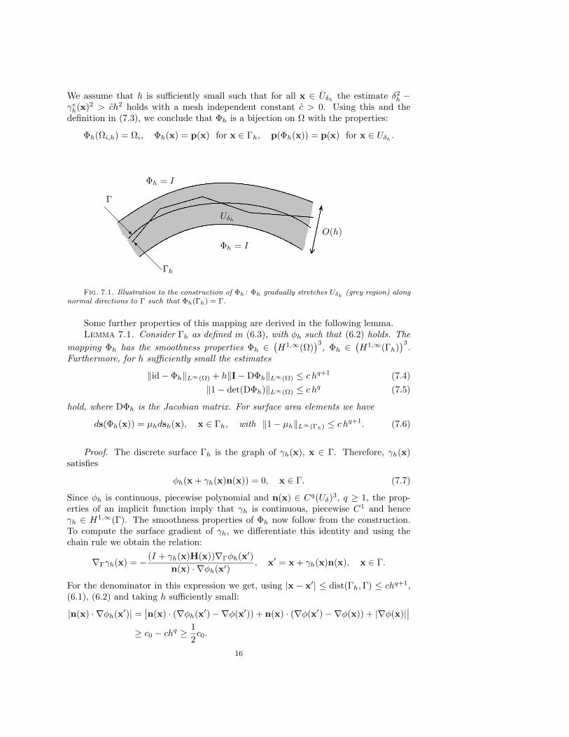
We assume that h is sufficiently small such that for all x ∈ Uδh the estimate δ2h −

γeh(x)2 > ch2 holds with a mesh independent constant c > 0. Using this and thedefinition in (7.3), we conclude that Φh is a bijection on Ω with the properties:

Φh(Ωi,h) = Ωi, Φh(x) = p(x) for x ∈ Γh, p(Φh(x)) = p(x) for x ∈ Uδh .

O(h)

Γh@@

@I

@@@R

Γ

Uδh

Φh = I

Φh = I

Fig. 7.1. Illustration to the construction of Φh: Φh gradually stretches Uδh (grey region) alongnormal directions to Γ such that Φh(Γh) = Γ.

Some further properties of this mapping are derived in the following lemma.Lemma 7.1. Consider Γh as defined in (6.3), with φh such that (6.2) holds. The

mapping Φh has the smoothness properties Φh ∈(H1,∞(Ω)

)3, Φh ∈

(H1,∞(Γh)

)3.

Furthermore, for h sufficiently small the estimates

‖id− Φh‖L∞(Ω) + h‖I−DΦh‖L∞(Ω) ≤ c hq+1 (7.4)

‖1− det(DΦh)‖L∞(Ω) ≤ c hq (7.5)

hold, where DΦh is the Jacobian matrix. For surface area elements we have

ds(Φh(x)) = µhdsh(x), x ∈ Γh, with ‖1− µh‖L∞(Γh) ≤ c hq+1. (7.6)

Proof. The discrete surface Γh is the graph of γh(x), x ∈ Γ. Therefore, γh(x)satisfies

φh(x + γh(x)n(x)) = 0, x ∈ Γ. (7.7)

Since φh is continuous, piecewise polynomial and n(x) ∈ Cq(Uδ)3, q ≥ 1, the prop-erties of an implicit function imply that γh is continuous, piecewise C1 and henceγh ∈ H1,∞(Γ). The smoothness properties of Φh now follow from the construction.To compute the surface gradient of γh, we differentiate this identity and using thechain rule we obtain the relation:

∇Γγh(x) = − (I + γh(x)H(x))∇Γφh(x′)

n(x) · ∇φh(x′), x′ = x + γh(x)n(x), x ∈ Γ.

For the denominator in this expression we get, using |x − x′| ≤ dist(Γh,Γ) ≤ chq+1,(6.1), (6.2) and taking h sufficiently small:

|n(x) · ∇φh(x′)| =∣∣n(x) · (∇φh(x′)−∇φ(x′)) + n(x) · (∇φ(x′)−∇φ(x)) + |∇φ(x)|

∣∣≥ c0 − chq ≥

1

2c0.

16

For the nominator we use ∇Γφ(x) = 0 and (6.2) to get:

|∇Γφh(x′)| ≤ |∇Γ(φh(x′)− φ(x′))|+ |∇Γ(φ(x′)− φ(x))| ≤ chq.

From this and (6.5) we infer

‖γh‖L∞(Γ) + h‖∇Γγh‖L∞(Γ) ≤ c hq+1. (7.8)

The following surface area transformation property can be found in, e.g., [9, 10]:

µh(x)dsh(x) = ds(p(x)), x ∈ Γh,

µh(x) := (1− d(x)κ1(x))(1− d(x)κ2(x))n(x)Tnh(x),

with κ1, κ2 the nonzero eigenvalues of the Weingarten map and nh the unit normal onΓh. Note that Φh(x) = p(x) on Γh holds. From (6.2) we get ‖1−µh‖L∞(Γh) ≤ chq+1.

Hence, the result in (7.6) holds. For the term l(x) :=δ2h−d(x)2

δ2h−γeh(x)2

, with x ∈ Uδh , used

in (7.3) we have ‖l‖L∞(Uδh ) ≤ c and ‖∇l‖L∞(Uδh ) ≤ ch−1. Using these estimates and

(7.1), (7.8) we obtain ‖id − Φh‖L∞(Ω) ≤ chq+1 and ‖I − DΦh‖L∞(Ω) ≤ chq. Thisproves (7.4). The result in (7.5) immediately follows from (7.4).

7.2. Smooth extensions. For functions v on Γ we have introduced above thesmooth constant extension along normals, denoted by ve. Below we also need a smoothextension to Ωi,h of functions u defined on Ωi. This extension will also be denotedby ue. Note that u Φh defines an extension to Ωi,h. This extension, however, hassmoothness H1,∞(Ωi,h), which is not sufficient for the interpolation estimates that weuse further on. Hence, we introduce an extension ue, which is close to u Φh in thesense as specified in Lemma 7.2 and is more regular.

As mentioned above, we make the smoothness assumption Γ ∈ Ck+1, where k isthe degree of the polynomials used in the finite element space, cf. (6.6). We denoteby Ei a linear bounded extension operator Hk+1(Ωi)→ Hk+1(R3) (see Theorem 5.4in [33]). This operator satisfies

‖Eiu‖Hm(R3) ≤ c‖u‖Hm(Ωi) ∀ u ∈ Hk+1(Ωi), m = 0, . . . , k + 1, i = 1, 2. (7.9)

For a piecewise smooth function u ∈ Hk+1(Ω1 ∪ Ω2), we denote by ue its “transfor-mation” to a piecewise smooth function ue ∈ Hk+1(Ω1,h ∪ Ω2,h) defined by

ue =

E1(u|Ω1) in Ω1,h

E2(u|Ω2) in Ω2,h.

(7.10)

The next lemma quantifies in which sense this function ue is close to u Φh.Lemma 7.2. The following estimates hold for i = 1, 2:

‖u Φh − ue‖Ωi,h ≤ chq+1‖u‖H1(Ωi), (7.11)

‖(∇u) Φh −∇ue‖Ωi,h ≤ chq+1‖u‖H2(Ωi), (7.12)

‖u Φh − ue‖Γh ≤ chq+1‖u‖H2(Ωi), (7.13)

for all u ∈ H2(Ωi).Proof. Without loss of generality we consider i = 1. Note that uΦh = E1(u|Ω1

)Φh in Ω1,h and ue = E1(u|Ω1) in Ω1,h. To simplify the notation, we write u1 =

17

E1(u|Ω1) ∈ H1(R3). We use that Φh = id and u = ue on Ω \ U δh and transform to

local coordinates in Uδh using the co-area formula:

‖u Φh − ue‖2Ω1,h= ‖u1 Φh − u1‖2Ω1,h

= ‖u1 Φh − u1‖2Ω1,h∩Uδh

=

∫Γ

∫ γh

−δh(u1 Φh − u1)2|∇φ|−1dr ds.

(7.14)

In local coordinates the mapping Φh can be represented as Φh(s, r) = (s, ps(r)), with

ps(r) = r − δ2h − r2

δ2h − γh(s)2

γh(s).

The function ps satisfies |ps(r)− r| ≤ chq+1. We use the identity

(u1 Φh − u1)(s, r) =

∫ ps(r)

r

r · ∇u1(s, t)dt, r =Φh(s, r)− (s, r)

|Φh(s, r)− (s, r)|. (7.15)

Due to (7.14), (7.15), the Cauchy inequality and |∇φ| ≥ c0 > 0 on Uδ, we get

‖u1 Φh − u1‖2Ω1,h≤ c

∫Γ

∫ γh

−δh|ps(r)− r|

∫ ps(r)

r

|∇u1(s, t)|2 |dt| dr ds

≤ chq+1

∫Γ

∫ γh

−δh

∫ r+chq+1

r−chq+1

|∇u1(s, t)|2 dt dr ds.(7.16)

Let χ[−chq+1,chq+1] be the characteristic function on [−chq+1, chq+1] and define g(t) =|∇u1(s, t)|2 for t ∈ [−δh − chq+1, γh + chq+1], g(t) = 0, t /∈ [−δh − chq+1, γh + chq+1].Applying the L1-convolution inequality we get

∫ γh

−δh

∫ r+chq+1

r−chq+1

|∇u1(s, t)|2 dtdr ≤ c∫ ∞−∞

∫ ∞−∞

χ[−chq+1,chq+1](r − t)g(t) dt dr

≤ c‖χ[−chq+1,chq+1]‖L1(R)‖g‖L1(R) ≤ chq+1

∫ γh+chq+1

−δh−chq+1

|∇u1(s, t)|2 dt,

and using this in (7.16) yields

‖u1 Φh − u1‖2Ω1,h≤ ch2q+2

∫Γ

∫ γh+chq+1

−δh−chq+1

|∇E1(u|Ω1)(s, t)|2 dr ds

≤ c h2q+2‖E1(u|Ω1)‖2H1(R3) ≤ c h2q+2‖u‖2H1(Ω1).

For deriving the estimate (7.12) we note that (∇u) Φh = (Ei((∇u)|Ωi) ) Φh =(∇(Ei(u|Ωi)) ) Φh = (∇u1) Φh in Ωi,h. Hence we have

‖(∇u) Φh −∇ue‖Ω1,h= ‖(∇u1) Φh −∇u1‖Ω1,h

.

We can repeat the arguments used above, with u1 replaced by ∂u1

∂xj, j = 1, 2, 3, and

thus obtain the estimate (7.12).

18

We continue to work in local coordinates and estimate the surface integral on theleft-hand side of (7.13) using the Cauchy inequality and ‖γh‖L∞(Γ) ≤ chq+1:

‖u1 Φh−u1‖2Γh =

∫Γ

(u1 − u1 Φ−1h )2(s, 0)µ−1

h ds =

∫Γ

[u1(s, 0)− u1(s, γh(s))]2µ−1h ds

=

∫Γ

(∫ γh

0

r · ∇u1(s, t)dt

)2

µ−1h ds ≤ c

∫Γ

|γh|∫ γh

0

|∇u1(s, t)|2 |dt| ds

≤ chq+1

∫Γ

∫ γh

0

|∇u1(s, t)|2 |dt| ds ≤ chq+1‖u1‖2H1(Uhq+1 ).

Here Uhq+1 is a tubular neighborhood of Γ of width O(hq+1) such that Γh ⊂ Uhq+1 .Now we apply the following result, proven in Lemma 4.10 in [15]:

‖w‖2Uhq+1≤ chq+1‖w‖2H1(R3) for all w ∈ H1(R3).

We let w = ∇u1 (componentwise) and use ‖E1(u|Ω1)‖H2(R3) ≤ c‖u‖H2(Ω1) to prove

(7.13).

7.3. Approximate Galerkin orthogonality. Due to the geometric errors, i.e.,approximation of Ωi by Ωi,h and of Γ by Γh, there is a so-called variational crime andonly an approximate Galerkin orthogonality relation holds. In this section we derivebounds for the deviation from orthogonality. The analysis is rather technical but theapproach is similar to related analyses from the literature, e.g., [10, 9, 4].

Let (u, v) ∈ V be the solution of the weak formulation (4.2) and (uh, vh) ∈ Vh

the discrete solution of (6.10). We take an arbitrary finite element test function(η, ζ) ∈ Vh. We use (η, ζ) Φ−1

h ∈ V as a test function in (4.2) and then obtain theapproximate Galerkin relation:

ah((ue − uh, ve − vh); (η, ζ))

= ah((ue, ve); (η, ζ))− a((u, v); (η, ζ) Φ−1h ) (7.17)

+ (f, η Φ−1h )Ω + (g, ζ Φ−1

h )Γ − (fh, η)Ω − (gh, ζ)Γh . (7.18)

In the analysis of the right-hand side of this relation we have to deal with full andtangential gradients∇(ηΦ−1

h ), ∇Γ(ζΦ−1h ). For the full gradient in the bulk domains

one finds

∇(η Φ−1h )(x) = DΦh(y)−T∇η(y), x ∈ Ω, y := Φ−1

h (x). (7.19)

To handle the tangential gradient, a more subtle approach is required because onehas to relate the tangential gradient ∇Γ to ∇Γh . Let nh(y), y ∈ Γh, denote theunit normal on Γh (defined a.e. on Γh). Furthermore, P(x) = I − n(x) ⊗ n(x)(x ∈ Uδ), Ph(y) = I − nh(y) ⊗ nh(y) (y ∈ Γh). Recall that ∇Γu(x) = P(x)∇u(x),∇Γhu(y) = Ph(y)∇u(y). We use the following relation, given in, e.g., [10]: forw ∈ H1(Γ) it holds

∇Γw(p(y)) = B(y)∇Γhwe(y) a.e. on Γh,

B(y) = (I− d(y)H(y))−1Ph(y), Ph(y) := I− nh(y)⊗ n(y)

nh(y) · n(y).

(7.20)

From the construction of the bijection Φh : Γh → Γ it follows that (ζΦ−1h )e(y) = ζ(y)

holds for all y ∈ Γh. Application of (7.20) yields an interface analogon of the relation

19

(7.19):

∇Γ(ζ Φ−1h )(x) = B(y)∇Γhζ(y), x ∈ Γ,y = Φ−1

h (x) ∈ Γh. (7.21)

The mapping Φh equals the identity outside the (small) tubular neighborhood Uδh .In the analysis we want to make use of the fact that the width behaves like δh = ch.For this, we again make use of the result in Lemma 4.10 in [15]:

‖w‖Uδh∩Ωi ≤ ch12 ‖w‖H1(Ωi) for all w ∈ H1(Ωi), (7.22)

where c depends only on Ωi. Using properties of Φh, i.e. Φh(Uδh ∩ Ωi,h) = Uδh ∩ Ωi,and (7.19) we thus get, with Jh = det(DΦh):

‖w‖Uδh∩Ωi,h = ‖wΦ−1h J

− 12

h ‖Uδh∩Ωi ≤ ch12 ‖wΦ−1

h ‖H1(Ωi) ≤ ch12 ‖w‖H1(Ωi,h), (7.23)

for all w ∈ H1(Ωi,h), with a constant c independent of w and h.

We introduce a convenient compact notation for the approximate Galerkin rela-tion. We use U := (u, v) = (u1, u2, v), and similarly Ue = (ue, ve), Uh := (uh, vh) ∈Vh, Θ = (η, ζ) ∈ H1(Ω1,h ∪ Ω2,h)×H1(Γh). Furthermore

Fh(Θ) := ah(Ue; Θ)− a(U ; Θ Φ−1h ).

For the right-hand side in the discrete problem (6.10) we set

fh := Jhf Φh, gh := µhg Φh, (7.24)

with Jh := det(DΦh) and µh as in (7.6). We make this choice, because then theconsistency terms in (7.18) vanish and the approximate Galerkin relation takes theform

ah(Ue − Uh; Θh) = Fh(Θh) for all Θh ∈ Vh. (7.25)

The choice (7.24) requires explicit knowledge of the transformation Φh, which maynot be practical. We comment on alternatives in Remark 3.In Lemma 7.3 we derive a bound for the functional Fh.

Lemma 7.3. For m = 0 and m = 1 the following estimate holds:

|Fh(Θ)| =∣∣ah(Ue; Θ)− a(U ; Θ Φ−1

h )∣∣

≤ chq+m(‖u‖H2(Ω1∪Ω2) + ‖v‖H1(Γ)

)(‖η‖H1+m(Ω1,h∪Ω2,h) + ‖ζ‖H1(Γh)

)for all U = (u, v) ∈ H2(Ω1∪Ω2)×H1(Γ), Θ = (η, ζ) ∈ H1+m(Ω1,h∪Ω2,h)×H1(Γh).

Proof. Take U = (u, v) ∈ H2(Ω1 ∪ Ω2) ×H1(Γ) and Θ = (η, ζ) ∈ H1+m(Ω1,h ∪Ω2,h)×H1(Γh). Denote Jh = det(DΦh). Using the definitions of the bilinear forms,

20

the relations (7.19), (7.20), (7.21) and an integral transformation rule we get

ah(Ue; Θ)− a(U ; Θ Φ−1h ) = ah((ue, ve); (η, ζ))− a((u, v); (η, ζ) Φ−1

h ) (7.26)

=

2∑i=1

[(νi∇ue,∇η)Ωi,h − (νi∇u Φh, Jh(DΦh)−T∇η)Ωi,h

](7.27)

+

2∑i=1

1

2

[(wh · ∇ue, η)Ωi,h − ((w · ∇u) Φh, Jhη)Ωi,h (7.28)

− (wh · ∇η, ue)Ωi,h +((w Φh) · (DΦh)−T∇η, Jhu Φh

)Ωi,h

](7.29)

+ νΓ(∇Γhve,∇Γhζ)Γh − νΓ(µhB

TB∇Γhve,∇Γhζ)Γh (7.30)

+1

2

[(wh · ∇Γhv

e, ζ)Γh − (µh(w Φh) ·B∇Γhve, ζ)Γh (7.31)

− (wh · ∇Γhζ, ve)Γh + (µh(w Φh) ·B∇Γhζ, v

e)Γh

](7.32)

+

2∑i=1

[(uei − qive, ηi −Kζ)Γh − ((ui − qiv) Φh, µh(ηi −Kζ))Γh

]. (7.33)

In this expression the different terms correspond to bulk diffusion, bulk convection,surface diffusion, surface convection and adsorption, respectively. We derive boundsfor these terms. We start with the bulk diffusion term in (7.27). Using the estimatesderived in the Lemmas 7.1, 7.2 we get

2∑i=1

∣∣∣(νi∇ue,∇η)Ωi,h − (νi∇u Φh, Jh(DΦh)−T∇η)Ωi,h

∣∣∣≤

2∑i=1

νi[|(∇(ue − u Φh), Jh(DΦh)−T∇η)Ωi,h |+ |(∇ue, (I− Jh(DΦh)−T )∇η)Ωi,h |

]≤ c

2∑i=1

[hq+1‖u‖H2(Ωi)‖∇η‖Ωi,h + hq‖ue‖H1(Ωi,h)‖∇η‖Ωi,h

](7.34)

≤ chq‖u‖H2(Ω1∪Ω2)‖η‖H1(Ω1,h∪Ω2,h). (7.35)

If η ∈ H2(Ω1,h ∪ Ω2,h) we can modify the estimate (7.34) as follows. Note thatJh(DΦh)−T = I on Ωi,h \ Uδh . Hence, using (7.23) we get

|(∇ue, (I− Jh(DΦh)−T )∇η)Ωi,h | = |(∇ue, (I− Jh(DΦh)−T )∇η)Uδh∩Ωi,h |≤ chq‖∇ue‖Uδh∩Ωi,h‖∇η‖Uδh∩Ωi,h ≤ chq+1‖ue‖H2(Ωi,h)‖η‖H2(Ωi,h)

≤ chq+1‖u‖H2(Ωi)‖η‖H2(Ωi,h).

(7.36)

Thus, instead of (7.35) we then obtain the upper bound

chq+1‖u‖H2(Ω1∪Ω2)‖η‖H2(Ω1,h∪Ω2,h).

21

For the bulk convection term in (7.28)-(7.29) we get

2∑i=1

1

2

∣∣(wh · ∇ue, η)Ωi,h − ((w · ∇u) Φh, Jhη)Ωi,h

∣∣+

1

2

∣∣(wh · ∇η, ue)Ωi,h −((w Φh) · (DΦh)−T∇η, Jhu Φh

)Ωi,h

∣∣≤

2∑i=1

1

2

∣∣(wh · ∇ue − (w · ∇u) Φh, Jhη)Ωi,h

∣∣+1

2

∣∣(wh · ∇ue, (1− Jh)η)Ωi,h

∣∣+

1

2

∣∣(wh − (w Φh) · (DΦh)−T∇η, Jhu Φh)Ωi,h

∣∣+1

2

∣∣(wh · ∇η, ue − Jhu Φh)Ωi,h

∣∣The difference wh −w Φh can be bounded using the assumption that the original(unscaled) velocity w is sufficiently smooth, w ∈ H1,∞(Ω). Using this, the relation(7.15) and the definition of wh we get ‖wh−w Φh‖L∞(Ωi,h) ≤ chq+1. The first termon the right-hand side above can be bounded using

‖wh · ∇ue − (w · ∇u) Φh‖Ωi,h = ‖wh · ∇ue − (w Φh) · (∇u Φh)‖Ωi,h≤ ‖(wh −w Φh) · ∇ue‖Ωi,h + ‖(w Φh) · (∇ue −∇u Φh)‖Ωi,h≤ chq+1‖u‖H2(Ωi),

where in the last step we used results from the Lemmas 7.1, 7.2. The other threeterms can be estimated by using ‖1 − Jh‖L∞(Ω) ≤ chq, ‖I − (DΦh)−T ‖L∞(Ω) ≤ chq

and ‖ue − u Φh‖Ωi,h ≤ chq+1‖u‖H1(Ωi). Thus we get a bound

2∑i=1

1

2

∣∣(wh · ∇ue, η)Ωi,h − ((w · ∇u) Φh, Jhη)Ωi,h

∣∣+

1

2

∣∣(wh · ∇η, ue)Ωi,h −((w Φh) · (DΦh)−T∇η, Jhu Φh

)Ωi,h

∣∣≤ chq‖u‖H2(Ω1∪Ω2)‖η‖H1(Ω1,h∪Ω2,h).

If η ∈ H2(Ω1,h ∪ Ω2,h) we can apply an argument very similar to the one in (7.36)and obtain the following upper bound for the bulk convection term:

chq+1‖u‖H2(Ω1∪Ω2)‖η‖H2(Ω1,h∪Ω2,h).

For the surface diffusion term in (7.30) we introduce, for y ∈ Γh, the matrix A(y) :=Ph(y)

(I − µh(y)B(y)TB(y)

)Ph(y). Using |d(y)| ≤ chq+1, |1 − µh(y)| ≤ chq+1 and

PhPh = Ph we get ‖A‖L∞(Γh) ≤ chq+1 and thus:

νΓ

∣∣(∇Γhve,∇Γhζ)Γh − (µhB

TB∇Γhve,∇Γhζ)Γh

∣∣ = νΓ

∣∣(A∇Γhve,∇Γhζ)Γh

∣∣≤ ‖A‖L∞(Γh)‖∇Γhv

e‖Γh‖∇Γhζ‖Γh ≤ chq+1‖v‖H1(Γ)‖ζ‖H1(Γh).

For the derivation of a bound for the surface convection term in (7.31)-(7.32) weintroduce w := Ph(wh − µhBT (w Φh)). Using the results in Lemmas 7.1, 7.2 andPw = w it follows that

‖w‖L∞(Γh) ≤ ‖Ph(wh −w Φh)‖L∞(Γh) + ‖Ph(I− µhBT )(w Φh)‖L∞(Γh)

≤ c‖Ph(I− PT )P‖L∞(Γh) + chq+1 ≤ c‖Phn‖L∞(Γh)‖Pnh‖L∞(Γh) + chq+1

= c‖(Ph −P)n‖L∞(Γh)‖(P−Ph)nh‖L∞(Γh) + chq+1

≤ c‖Ph −P‖2L∞(Γh) + chq+1.

22

Using

|nh(y)− n(y)| = |nh(y)− n(p(y))| =∣∣∣∣ ∇φh(y)

|∇φh(y)|− ∇φ(p(y))

|∇φ(p(y))|

∣∣∣∣in combination with |y− p(y)| ≤ chq+1 and the approximation error bound (6.2) weget ‖P−Ph‖L∞(Γh) ≤ chq. Hence, for the surface convection term in (7.31) we obtain∣∣(wh · ∇Γhv

e, ζ)Γh − (µh(w Φh) ·B∇Γhve, ζ)Γh

∣∣= |(w · ∇Γhv

e, ζ)Γh

∣∣ ≤ ‖w‖L∞(Γh)‖∇Γhve‖Γh‖ζ‖Γh ≤ chq+1‖v‖H1(Γ)‖ζ‖H1(Γh).

The term in (7.32) can be bounded in the same way. Finally we consider the adsorption-desorption term in (7.33). Using the results in Lemmas 7.1, 7.2 we get

2∑i=1

∣∣∣(uei − qive, ηi −Kζ)Γh − ((ui − qiv) Φh, µh(ηi −Kζ))Γh

∣∣∣≤

2∑i=1

∣∣(uei − µhui Φh, ηi −Kζ)Γh

∣∣+ qi∣∣((1− µh)ve, ηi −Kζ)Γh

∣∣≤ chq+1

2∑i=1

(‖ui‖H2(Ωi) + ‖v‖Γ

)(‖ηi‖Γh + ‖ζ‖Γh

).

≤ c hq+1(‖u‖H2(Ω1∪Ω2) + ‖v‖Γ)(‖η‖H1(Ω1,h∪Ω2,h) + ‖ζ‖Γh).

Combining these estimates for the terms in (7.27)-(7.33) completes the proof.

From the arguments in the proof above one easily sees that the bounds derivedin Lemma 7.3 also hold if in ah(·; ·) and a(·; ·) the arguments are interchanged. Thisproves the result in the following lemma, that we need in the L2-error analysis.

Lemma 7.4. The following estimate holds:∣∣ah(Θ;Ue)− a(Θ Φ−1h ;U)

∣∣≤ chq

(‖η‖H1(Ω1,h∪Ω2,h) + ‖ζ‖H1(Γh)

)(‖u‖H2(Ω1∪Ω2) + ‖v‖H1(Γ)

)for all U = (u, v) ∈ H2(Ω1 ∪ Ω2)×H1(Γ), Θ = (η, ζ) ∈ H1(Ω1,h ∪ Ω2,h)×H1(Γh).

As an immediate corollary of Lemma 7.3, the definition of Fh and the regularityestimate in Theorem 4.5 we obtain the following result.

Lemma 7.5. Assume that the solution (u, v) of (4.2) has smoothness u ∈ H2(Ω1∪Ω2), v ∈ H2(Γ). For m = 0 and m = 1 the following holds:

|Fh(Θ)| ≤ chq+m(‖f‖Ω + ‖g‖Γ)(‖η‖H1+m(Ω1,h∪Ω2,h) + ‖ζ‖H1(Γh)

)(7.37)

for all Θ = (η, ζ) ∈ H1+m(Ω1,h ∪ Ω2,h)×H1(Γh).

Remark 3. The consistency estimate in Lemma 7.5 is proved for the particularchoice of the finite element problem right-hand side as in (7.24). This choice simplifiesthe analysis because the terms in (7.18) vanish. Similar estimates, however, can beproved if fh and gh are chosen as generic smooth extensions of f ∈ H1(Ω1 ∪Ω2) andg ∈ L2(Γ). For example, one may set fh = fe, gh = ge|Γh − cf , where cf is such that

23

mean value condition is satisfied. In this case, the following estimate holds for theterms in (7.18):∣∣(f, η Φ−1

h )Ω + (g, ζ Φ−1h )Γ − (fe, η)Ω − (ge, ζ)Γh + (cf , ζ)Γh

∣∣≤ chq+1

(‖f‖H1(Ω1∪Ω2) + ‖g‖Γ

)(‖η‖H1(Ω1,h∪Ω2,h) + ‖ζ‖Γh

)for all (η, ζ) ∈ H1(Ω1,h ∪ Ω2,h) × H1(Γh). A proof of this estimate is given in thepreprint version of this paper [20]. The discretization error bounds in (7.40) and(8.3) hold for this alternative right-hand side choice, provided ‖f‖Ω is replaced by‖f‖H1(Ω1∪Ω2).

7.4. Discretization error bound in the Vh-norm. Based on the stability,continuity and approximate Galerkin properties presented in the previous sections,we derive a discretization error bound in the Vh norm. Due to the approximation ofthe interface the discrete solution Uh = (uh, vh) has a domain that differs from thatof the solution U = (u, v) to the continuous problem. Therefore, it is not appropriateto define the error as U −Uh. It is natural to define the discretization error either asUe−Uh, with functions defined on the domain corresponding to the discrete problem,or as U − Uh Φ−1

h , with functions defined on the domain corresponding to thecontinuous problem. We use the former definition. In the analysis we need suitableinterpolation operators, applicable to Ue. The function ue consists of the pair ue =(E1(u|Ω1

)|Ω1,h, E2(u|Ω2

)|Ω2,h) =: (ue1, u

e2), cf. (7.10). As is standard in analyses of

XFEM (or unfitted FEM) we define an interpolation based on the standard nodalinterpolation of the smooth extension in the bulk space V bulk

h . Let Ibulkh denote the

nodal interpolation in V bulkh (which consists of finite elements of degree k). We define

Ihue ∈ VΩ,h as follows:

Ihue =

([Ibulkh E1(u|Ω1

)]|Ω1,h, [Ibulk

h E2(u|Ω2)]|Ω2,h

).

The construction of this operator and interpolation error bounds for Ibulkh immediately

yield

‖Ihue − ue‖H1(Ω1,h∪Ω2,h) ≤ c hk‖u‖Hk+1(Ω1∪Ω2). (7.38)

For the interpolation of ve we use a similar approach, namely Ihve := [Ibulk

h ve]|Γh .

Here the interpolation operator Ibulkh is applied only on the tetrahedra that are inter-

sected by Γh. Interpolation error bounds for this operator are known in the literature,see, e.g., Theorem 4.2 in [31]:

‖Ihve − ve‖H1(Γh) ≤ c hk‖v‖Hk+1(Γ). (7.39)

Using these interpolation error bounds we obtain the following main theorem.Theorem 7.6. Let the solution (u, v) ∈ V of (4.4) be sufficiently smooth. For

the finite element solution (uh, vh) ∈ Vh the following error estimate holds:

‖(ue − uh, ve − vh)‖Vh≤ chk

(‖u‖Hk+1(Ω) + ‖v‖Hk+1(Γ)

)+ chq

(‖f‖Ω + ‖g‖Γ

),

(7.40)

where k is the degree of the finite element polynomials and q the geometry approxima-tion order defined in (6.2).

Proof. We use arguments similar to the second Strang’s lemma. Recalling thestability and continuity results from (6.11), (6.12), the consistency error bound in

24

Lemma 7.5 and the interpolation error bounds in (7.38), (7.39) we get, with IhUe =

(Ihue, Ihv

e):

‖IhUe − Uh‖Vh≤ C−1

st supΘh∈Vh

ah(IhUe − Uh; Θh)

‖Θh‖Vh

= C−1st sup

Θh∈Vh

(ah(IhUe − Ue; Θh)

‖Θh‖Vh

+ah(Ue − Uh; Θh)

‖Θh‖Vh

)≤ c

(‖IhUe − Ue‖Vh

+ supΘh∈Vh

Fh(Θh)

‖Θh‖Vh

)≤ c hk(‖u‖Hk+1(Ω) + ‖v‖Hk+1(Γ)) + chq(‖f‖Ω + ‖g‖Γ).

(7.41)

The desired result now follows by a triangle inequality and applying the interpolationerror estimates (7.38), (7.39) once more.

8. Error estimate in L2-norm. In this section we use a duality argument toshow higher order convergence of the unfitted finite element method in the L2 productnorm. As typical in the analysis of elliptic PDEs with Neumann boundary conditions,one considers the L2 norm in a factor space:

‖U‖L2/R = infγ∈R‖U − γ(q1, q2, 1)‖L2(Ω)×L2(Γ), for U ∈ L2(Ω)× L2(Γ),

and q1, q2 ∈ [0, 1] from (3.7). A similar norm can be defined on L2(Ω)× L2(Γh).Define the error Eh := (Ue−Uh)Φ−1

h ∈ L2(Ω)×L2(Γ). There is a constant γ ∈ Rsuch that Eh := Eh − γ(q1, q2, 1) satisfies the consistency condition (5.2). Accordingto Theorem 5.1 the dual problem: Find W ∈ Vα such that

a(Θ;W ) = (Eh,Θ)L2(Ω)×L2(Γ) for all Θ ∈ V, (8.1)

has the unique solution W = (w, z) ∈ H2(Ω1 ∪ Ω2)×H2(Γ), satisfying

‖w‖H2(Ω1∪Ω2) + ‖z‖H2(Γ) ≤ c‖Eh‖L2(Ω)×L2(Γ), (8.2)

with a constant c independent of Eh.Theorem 8.1. Let the assumptions in Theorem 7.6 and Theorem 5.1 be fulfilled.

For the finite element solution (uh, vh) ∈ Vh the following error estimate holds:

‖ue − uh, ve − vh‖L2/R ≤ chk+1(‖u‖Hk+1(Ω1∪Ω2) + ‖v‖Hk+1(Γ)

)+ chq+1

(‖f‖Ω + ‖g‖Γ

),

(8.3)

where k is the degree of the finite element polynomials and q the geometry approxima-tion order defined in (6.2).

Proof. First, let γopt := arg infγ∈R ‖Eh − γ(q1, q2, 1)‖L2(Ω)×L2(Γ). Observe thechain of estimates:

‖Ue − Uh‖L2/R ≤ ‖Ue − Uh − γopt(q1, q2, 1)‖L2(Ω)×L2(Γh)

= ‖(Ue − Uh − γopt(q1, q2, 1)) Φ−1h J

− 12

h ‖L2(Ω)×L2(Γ)

≤ c‖(Ue − Uh − γopt(q1, q2, 1)) Φ−1h ‖L2(Ω)×L2(Γ)

= c‖(Ue − Uh) Φ−1h − γopt(q1, q2, 1)‖L2(Ω)×L2(Γ)

= c ‖Eh‖L2/R ≤ c‖Eh‖L2(Ω)×L2(Γ).

25

We apply the standard duality argument and thus obtain:

‖Eh‖2L2(Ω)×L2(Γ) = a(Eh,W ) = a(Eh,W )

= a(Eh;W )− ah(Ue − Uh;W e) + ah(Ue − Uh;W e − IhW e)− ah(Ue − Uh; IhWe)

=[a(Eh;W )− ah(Ue − Uh;W e)

]+ ah(Ue − Uh;W e − IhW e) + Fh(IhW

e)

=[a(Eh;W )− ah(Ue − Uh;W e)

]+ ah(Ue − Uh;W e − IhW e)

+ Fh(IhWe −W e) + Fh(W e).

These terms can be estimated as follows. For the term between square brackets weuse Lemma 7.4 and (8.2):

|a(Eh;W )− ah(Ue − Uh;W e)| ≤ chq‖Ue − Uh‖Vh(‖w‖H2(Ω1∪Ω2) + ‖z‖H1(Γ))

≤ chq‖Ue − Uh‖Vh‖Eh‖L2(Ω)×L2(Γ)

For the second term we use continuity, the interpolation error bound and (8.2):

|ah(Ue − Uh;W e − IhW e)| ≤ ch‖Ue − Uh‖Vh(‖w‖H2(Ω1∪Ω2) + ‖z‖H2(Γ))

≤ ch‖Ue − Uh‖Vh‖Eh‖L2(Ω)×L2(Γ).

For the third term we use Lemma 7.5 with m = 0, the interpolation error bound and(8.2):

|Fh(IhWe −W e)| ≤ chq

(‖f‖Ω + ‖g‖Γ

)‖IhW e −W e‖Vh

≤ chq+1(‖f‖Ω + ‖g‖Γ

)‖Eh‖L2(Ω)×L2(Γ).

For the fourth term we use Lemma 7.5 with m = 1 and (8.2):

|Fh(W e)| ≤ chq+1(‖f‖Ω + ‖g‖Γ

)‖Eh‖L2(Ω)×L2(Γ).

Combining these results and using the bound for ‖Ue − Uh‖Vhof Theorem 7.6 com-

pletes the proof.

9. Numerical results. We consider the stationary coupled bulk-interface con-vection diffusion problem (3.3) in the domain Ω = [−1.5, 1.5]3 and with the unitsphere Γ = x ∈ Ω : ‖x‖2 = 1 as interface. For the velocity field we take a rotatingfield in the x-z plane: w = 1

10 (z, 0,−x). This w satisfies the conditions (2.1) and(3.1), i.e., div w = 0 in Ω and w · n = 0 on Γ. On some parts of the boundary ∂Ωthe velocity field w is pointing inwards the domain, i.e., (3.2) does not hold. Hence,there are convective fluxes on ∂Ω and thus a Neumann boundary condition as in (3.3)is not natural. For this reason, and to simplify the implementation, we use Dirichletboundary conditions on ∂Ω. Note that in this case we do not need the additionalcondition (4.1) to obtain well-posedness. For the scaling constant we take K = 1.

9.1. Convergence study. In this experiment, the material parameters are cho-sen as ν1 = 0.5, ν2 = 1, νΓ = 1 and k1,a = 0.5, k2,a = 2, k1,d = 2, k2,d = 1. Thesource terms fi ∈ L2(Ω), i = 1, 2, and g ∈ L2(Γ) in (3.3) and the Dirichlet boundarydata are taken such that the exact solution of the coupled system is given by

v(x, y, z) = 3x2y − y3,

u1(x, y, z) = 2u2(x, y, z),

u2(x, y, z) = e1−x2−y2−z2v(x, y, z).

(9.1)

26

Note that the gauge condition (3.4) is satisfied for this choice of f and g. For the ini-tial triangulation, Ω is divided into 4×4×4 sub-cubes each consisting of 6 tetrahedra.This initial mesh is uniformly refined up to 4 times, yielding Th. The discrete interfaceΓh is obtained by linear interpolation of the signed distance function correspondingto Γ. We use the finite element spaces in (6.6)-(6.7) with k = 1, i.e., V bulk

h consists ofpiecewise linears on Th.For the representation of functions in the trace finite element spaces VΓ,h and Vi,h,cf. (6.7), we use the standard nodal basis functions in the bulk space V bulk

h . For VΓ,h

and Vi,h only those basis functions are used, the support of which has a nonzero inter-section with Γh and Ω1,h, respectively. Hence, the nodal finite element functions usedfor represented functions from the trace space VΓ,h are a subset of the basis functionsthat are used for representing functions from Vi,h. The resulting coupled linear systemis iteratively solved by a Generalized Conjugate Residual (GCR) method using a blockdiagonal preconditioner, where the bulk and interface systems are preconditioned bythe symmetric Gauss-Seidel method.

The numerical solution uh, vh after 2 grid refinements and the resulting interfaceapproximation Γh are shown in Figure 9.1.

Fig. 9.1. Numerical solutions vh on Γh and uh visualized on a cut plane z = 0 for refinementlevel 2.

The L2 and H1 errors for the bulk and interface concentration are given in Ta-bles 9.1 and 9.2. For computing the discretization error on the “discrete” domainsΩi,h and Γh we use u|Ωi,h := ui, i = 1, 2, v|Γh := v, with ui and v as in (9.1). Inthe column “order” we give the estimated p in the error behavior ansatz chp. Asexpected, first order convergence is obtained for the H1 errors of bulk and interfaceconcentration, cf. Theorem 7.6. The respective L2 errors are of second order, whichconfirms the theoretical findings in Theorem 8.1.

The number of GCR iterations to reach a residual norm below 10−10 are reportedin Table 9.2. Although, due to the small areas in certain cut elements, the condi-tion numbers of the stiffness matrices can be extremely large, we do not observe a

27

# ref. ‖u− uh‖L2(Ω) order ‖u− uh‖H1(Ω1,h∪Ω2,h) order

0 1.27E+0 — 6.07E+0 —1 4.39E-1 1.53 3.39E+0 0.842 1.28E-1 1.78 1.79E+0 0.923 3.34E-2 1.94 9.12E-1 0.984 8.47E-3 1.98 4.58E-1 0.99

Table 9.1L2 and H1 errors for bulk concentration uh on different refinement levels.

# ref. # iter. ‖v − vh‖L2(Γh) order ‖v − vh‖H1(Γh) order

0 29 6.75E-1 — 4.60E+0 —1 41 1.88E-1 1.85 2.30E+0 1.002 67 5.39E-2 1.80 1.01E+0 1.183 119 1.34E-2 2.01 5.15E-1 0.984 218 3.38E-3 1.99 2.52E-1 1.03

Table 9.2L2 and H1 errors for interface concentration vh and iteration numbers on different refinement

levels.

strong deterioration in the iteration numbers of the preconditioned Krylov solver. Theiteration numbers in Table 9.2 show a rather regular ∼ h−1 growth behavior.

9.2. Effect of small desorption. The theory presented indicates that both themodel and the discretization are stable if the desorption coefficients tend to zero. Forthe simpler case with only one bulk domain such a uniform stability result has notbeen derived in [4, 15]. The analysis of well-posedness in [15] for the case of one bulkdomain makes essential use of the assumption that the desorption coefficient is strictlypositive and the constants in the analysis may blow up if the desorption coefficienttends to zero. In the numerical experiments presented in [4, 15] only ka = kd = 1is considered. In applications one typically has 0 < kd ka. Therefore we includeresults of an experiment with a small or even vanishing desorption coefficient. Forthe bulk concentration, homogeneous Dirichlet boundary data on ∂Ω are chosen. Thesource terms are set to fi = 0, i = 1, 2 and g = 1, so bulk concentration can only begenerated by desorption of interface concentration from Γ. The material parametersare chosen as ν1 = 0.5, ν2 = 1, νΓ = 1 and k1,a = k2,a = k2,d = 1, k1,d = ε withε ≥ 0. We use the same initial triangulation as before. This initial mesh is uniformlyrefined 3 times, and the discrete problem is solved on this mesh for different values of ε,yielding solutions uεi,h ∈ Vi,h, vεh ∈ VΓ,h. Table 9.3 shows the mean bulk concentrationof uε1,h in Ω1,h,

u1,h(ε) := |Ω1,h|−1

∫Ω1,h

uε1,h dx,

28

kd,1 u1,h(kd,1)

1E+0 1.42E+001E-1 1.42E-011E-3 1.42E-031E-5 1.42E-051E-10 1.42E-10

0 1.37E-15

Table 9.3Mean bulk concentration in Ω1,h for different

values of the desorption coefficient kd,1 forrefinement level 3.

# ref. u1,h(10−3)

0 1.3191E-031 1.3865E-032 1.4088E-033 1.4153E-034 1.4171E-03

Table 9.4Mean bulk concentration in Ω1,h with desorp-

tion coefficient kd,1 = 10−3 for different re-finement levels.

for different values of the desorption coefficient k1,d = ε. We clearly observe a linearbehavior, which can be expected, based on the relation

k1,a

∫Γ

u1 ds =

∫Γ

u1 ds = k1,d

∫Γ

v ds,

that holds for the continuous solution u1, v (follows from the first and third equationin (3.3)). In the numerical experiments the discrete analogon of this relation turns outto be satisfied with value

∫Γhvh ds = 17.775 for all considered values of ε. For ε = 0

we have u1,h(0) = 1.37·10−15 which is due to round-off errors and the chosen tolerancetol = 10−14 of the iterative solver. Hence, in the discrete problem the (mean) bulkconcentration in Ω1 is very close to zero (which is the correct value from the continuousmodel), i.e, there is no “numerical leakage” of surfactant concentration through theinterface. The iteration numbers are essentially independent of ε (155 ± 1 iterationsfor the considered range of ε), indicating that the condition number of the resultingpreconditioned system matrix is robust w.r.t. k1,d → 0. These results illustrate the

well-posedness of the model and the stability of the discretization for k1,d ↓ 0.We now fix the value ε = 10−3 and change the number of uniform grid refinements,

obtaining different mesh sizes hi, i = 0, 1, . . . , 4. The obtained values of u1,hi(10−3)are given in Table 9.4. These numbers show a linear convergence behavior with acontraction factor ∼ 0.3, which indicates that we have stable (almost second order)convergence w.r.t h. On refinement level 3 we have an estimated relative error ofapproximately 2 · 10−3.

10. Discussion and outlook. In this paper a coupled system of elliptic partialdifferential equations is studied, in which two advection-diffusion equations in bulksubdomains are coupled, via adsorption-desorption terms, with an advection-diffusionequation on the interface between these bulk domains. This system of equations ismotivated by models for surfactant transport in two-phase flow problems. A mainresult is the well-posedness of a certain weak formulation of this system of equations.We introduce an unfitted finite element method for the discretization of this problem.The method uses three trace spaces of one standard bulk finite element space. Theinterface is approximated by the zero level of a finite element function. For this finiteelement function and for the finite element functions used in the bulk space piecewiselinears as well as higher order polynomials can be used. For this discretization methodoptimal error bounds are derived. We consider the following topics to be of interestfor future research.

29

The unfitted finite element discretization leads to linear systems of equations thatmay become ill-conditioned. The discretization method treated in this paper can becombined with a stabilization procedure as recently presented in [4]. For the case ofone bulk domain the method treated in this paper is the same as the unstabilizedmethod in [4]. The stabilization procedure considered in [4] does not rely on thefact that there is only one bulk domain, and looking at the analysis of the stabilizedmethod in [4] we expect that it will work for the case with two bulk domains, too.The use of an unfitted finite element technique becomes particularly attractive fortime dependent problems with an evolving interface. In the applications that we havein mind (surfactants in two-phase incompressible flow) such time dependent problemsare highly relevant. Hence, the extension of the method studied in this paper to atime- dependent coupled system as in (2.8) is an interesting topic. Such an extensionmay be based on space-time trace finite element methods that are studied in the recentpapers [27, 25], which deal with advection-diffusion equations on evolving surfaces,but without a coupling to a bulk phase.Finally we note that if for the interface approximation a finite element polynomialof degree q ≥ 2 is used, the zero level of this function is not directly available. Asuitable quadrature for approximating integrals of Γh has to be developed. This isnot straightforward. For special cases in which the distance function to Γ is known,computable parametrizations as treated in [9] can be used. A more general approachhas recently been presented in [18]. A similar quadrature problem arises for thetetrahedra in the bulk domain that are cut by the interface Γh.

REFERENCES

[1] A. Alphonso, C. Elliott, and B. Stinner, An abstract framework for parabolic pdes onevolving spaces, preprint, 2014. arXiv:1403.4500.

[2] A. Bonito, R. Nochetto, and M. Pauletti, Dynamics of biomembranes: effect of the bulkfluid, Math. Model. Nat. Phenom., 6 (2011), pp. 25–43.

[3] E. Burman and P. Hansbo, Fictitious domain finite element methods using cut elements: II.a stabilized nitsche method, Appl. Numer. Math., 62 (2012), pp. 328–341.

[4] E. Burman, P. Hansbo, M. Larson, and S. Zahedi, Cut finite element methods for coupledbulk-surface problems, preprint, 2014. arXiv:1403.6580.

[5] K.-Y. Chen and M.-C. Lai, A conservative scheme for solving coupled surface-bulk convection-diffusion equations with an application to interfacial flows with soluble surfactant, J.Comp. Phys., 257 (2014), pp. 1–18.

[6] J. Chessa and T. Belytschko, An extended finite element method for two-phase fluids, ASMEJournal of Applied Mechanics, 70 (2003), pp. 10–17.

[7] R. Clift, J. Grace, and M. Weber, Bubbles, Drops and Particles, Dover, Mineola, 2005.[8] K. Deckelnick, C. Elliott, and T. Ranner, Unfitted finite element methods using bulk

meshes for surface partial partial differential equations, preprint, 2013. arXiv:1312.2905.[9] A. Demlow, Higher-order finite element methods and pointwise error estimates for elliptic

problems on surfaces, SIAM J. Numer. Anal., 47 (2009), pp. 805–827.[10] A. Demlow and G. Dziuk, An adaptive finite element method for the Laplace-Beltrami op-

erator on implicitly defined surfaces, SIAM Journal on Numerical Analysis, 45 (2007),pp. 421–442.

[11] A. Demlow and M. Olshanskii, An adaptive surface finite element method based on volumemeshes, SIAM J. Numer. Anal., 50 (2012), pp. 1624–1647.

[12] M. Do-Quang, G. Amberg, and C.-O. Petterson, Modeling of the adsorption kineticsand the convection of surfactants in a weld pool, Journal of heat transfer, 130 (2008),pp. 092102–1.

[13] G. Dziuk and C. Elliott, Finite element methods for surface pdes, Acta Numerica, 22 (2013),pp. 289–396.

[14] C. Eggleton and K. Stebe, An adsorption-desorption-controlled surfactant on a deformingdroplet, Journal of colloid and interface science, 208 (1998), pp. 68–80.

[15] C. Elliott and T. Ranner, Finite element analysis for a coupled bulk-surface partial differ-

30

ential equation, IMA J. Numer. Anal., 33 (2013), pp. 377–402.[16] A. Ern and J.-L. Guermond, Theory and practice of finite elements, Springer, New York,

2004.[17] T. Fries and T. Belytschko, The generalized/extended finite element method: An overview

of the method and its applications, Int. J. Num. Meth. Eng., 84 (2010), pp. 253–304.[18] J. Grande and A. Reusken, A higher order finite element method for partial differential

equations on surfaces, Preprint 403, IGPM RWTH Aachen University, 2014.[19] P. Grisvard, Elliptic problems in nonsmooth domains, Pitman, Boston, 1985.[20] S. Groß, M. A. Olshanskii, and A. Reusken, A trace finite element method for a class

of coupled bulk-interface transport problems, Preprint 28, SC&NA, University of Houston,2014.

[21] S. Groß and A. Reusken, Numerical Methods for Two-phase Incompressible Flows, Springer,Berlin, 2011.

[22] A. Hansbo and P. Hansbo, An unfitted finite element method, based on nitsche’s method, forelliptic interface problems, Comput. Methods Appl. Mech. Engrg., 191 (2002), pp. 5537–5552.

[23] , A finite element method for the simulation of strong and weak discontinuities in solidmechanics, Comput. Methods Appl. Mech. Engrg., 193 (2004), pp. 3523–3540.

[24] M. Olshanskii and A. Reusken, A finite element method for surface PDEs: matrix properties,Numer. Math., 114 (2009), pp. 491–520.

[25] M. Olshanskii and A. Reusken, Error analysis of a space-time finite element method forsolving PDEs on evolving surfaces, SIAM J. Numer. Anal., 52 (2014), pp. 2092–2120.

[26] M. Olshanskii, A. Reusken, and J. Grande, A finite element method for elliptic equationson surfaces, SIAM J. Numer. Anal., 47 (2009), pp. 3339–3358.

[27] M. Olshanskii, A. Reusken, and X. Xu, An Eulerian space-time finite element method fordiffusion problems on evolving surfaces, SIAM J. Numer. Anal., 52 (2014), pp. 1354–1377.

[28] M. Olshanskii, A. Reusken, and X. Xu, A stabilized finite element method for advection-diffusion equations on surfaces, IMA Journal of Numerical Analysis, 34 (2014), pp. 732–758.

[29] M. Olshanskii and D. Safin, A narrow-band unfitted finite element method for elliptic pdesposed on surfaces, Preprint 26, SC&NA, University of Houston, 2014.

[30] F. Ravera, M. Ferrari, and L. Liggieri, Adsorption and partition of surfactants in liquid-liquid systems, Advances in Colloid and Interface Science, 88 (2000), pp. 129–177.

[31] A. Reusken, Analysis of trace finite element methods for surface partial differential equations,IMA J. Numer. Anal. doi: 10.1093/imanum/dru047, (2014).

[32] S. Tasoglu, U. Demirci, and M. Muradoglu, The effect of soluble surfactant on the transientmotion of a buoyancy-driven bubble, Physics of fluids, 20 (2008), pp. 040805–1.

[33] J. Wloka, Partial Differential Equations, Cambridge University Press, Cambridge, 1987.

31