application of the immersed boundary method to particle...

Application of the Immersed Boundary Method to particle-laden andp

bubbly flows

T. Kempe, B. Vowinckel, S. Schwarz, C. Santarelli, J. Fröhlich

Institute of Fluid MechanicsInstitute of Fluid MechanicsTU Dresden, Germany

EUROMECH Colloquium 549, Leiden, 17-19 June 2013

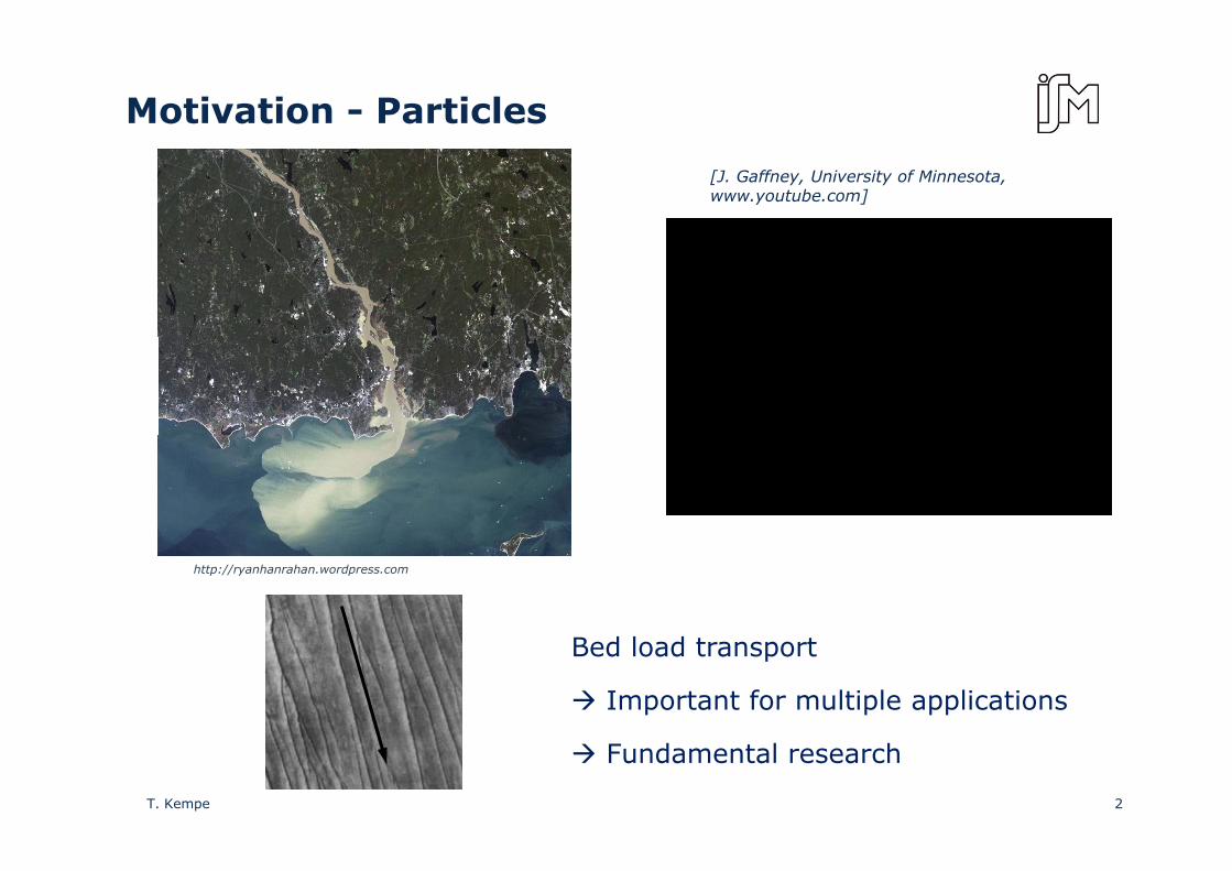
Motivation - Particles

[J. Gaffney, University of Minnesota, www.youtube.com]

http://ryanhanrahan.wordpress.com

Bed load transport

Important for multiple applications

Fundamental research

2T. Kempe

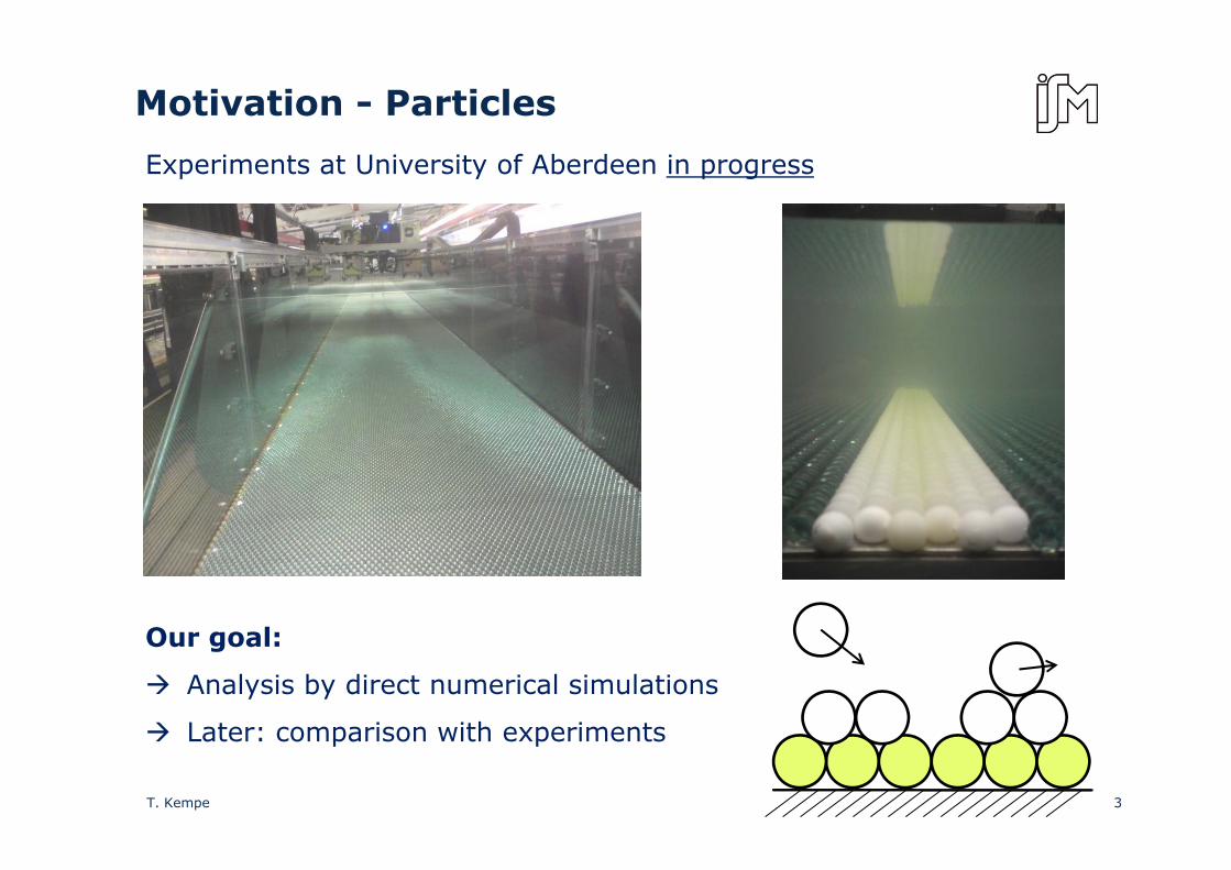
Motivation - Particles

Experiments at University of Aberdeen in progress

Our goal:Our goal:

Analysis by direct numerical simulations

Later: comparison with experimentsLater: comparison with experiments

3T. Kempe

Motivation - Bubbles

Our goals:

Bubble - turbulence interactionBubble turbulence interaction

Bubbles in MHD flows

Formation of metal foamsFormation of metal foams

X R • X-Ray measurements [Boden EPM 2009]

• Ar in GaInSn • Ar in GaInSn • No magnetic field

4T. Kempe

1. Basic fluid solver and IBM

2. Collision modeling

3. Bed load transportp

4. Bubble laden flows

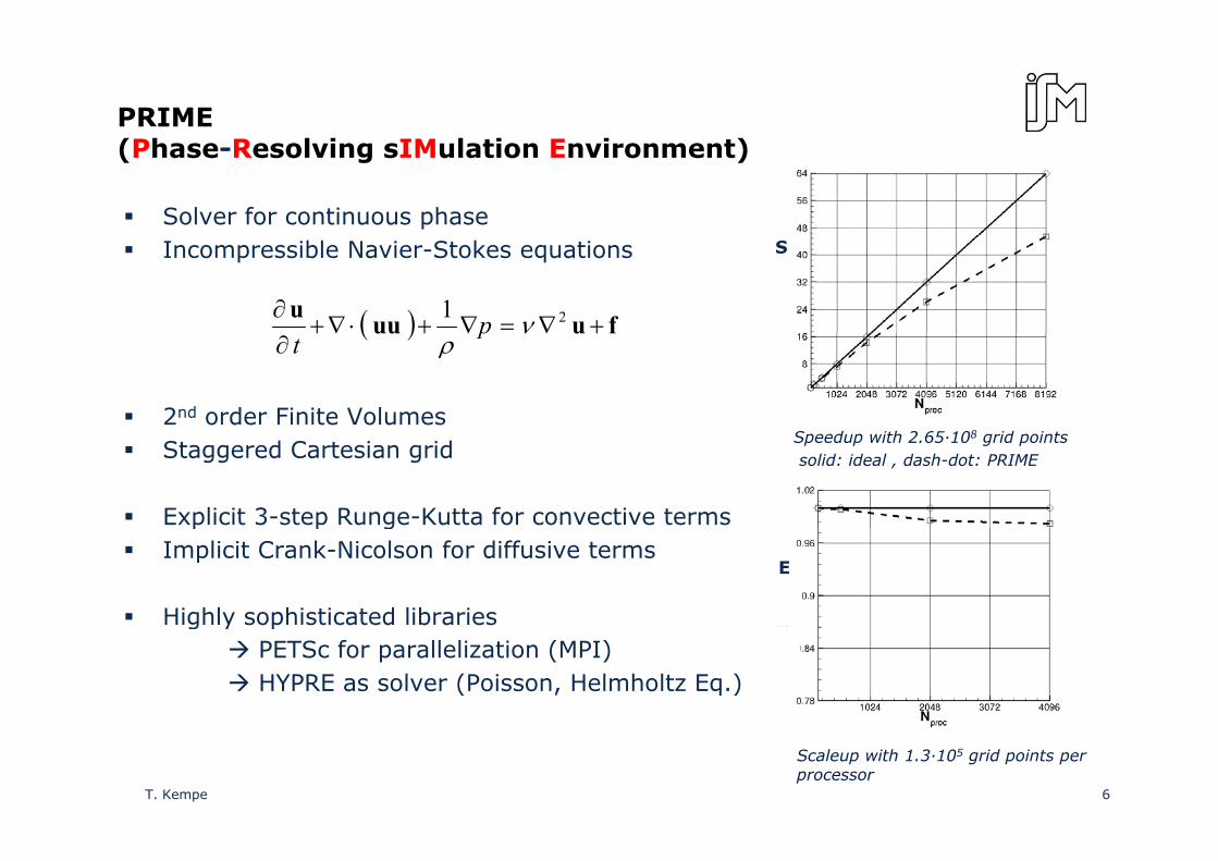
PRIME(Phase-Resolving sIMulation Environment)

Solver for continuous phaseIncompressible Navier-Stokes equations

( ) fuuuu+∇=∇+⋅∇+

∂ 21 νp

S

2nd order Finite Volumes

( ) fuuu +∇∇+∇+∂

νρ

pt

8

Staggered Cartesian grid

Explicit 3-step Runge-Kutta for convective terms

Speedup with 2.65·108 grid pointssolid: ideal , dash-dot: PRIME

p p gImplicit Crank-Nicolson for diffusive terms

Highly sophisticated libraries

E

g y pPETSc for parallelization (MPI)HYPRE as solver (Poisson, Helmholtz Eq.)

6

Scaleup with 1.3·105 grid points per processor

T. Kempe

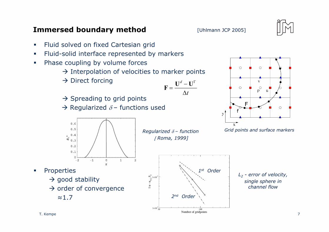
Immersed boundary method [Uhlmann JCP 2005]

Fluid solved on fixed Cartesian gridFluid-solid interface represented by markersPhase coupling by volume forcesPhase coupling by volume forces

Interpolation of velocities to marker pointsDirect forcing d −

=ΓUUF

Spreading to grid points Regularized δ – functions used F

f

tΔF

Grid points and surface markersRegularized δ – function[ Roma, 1999]

P tiPropertiesgood stability order of convergence

L2 - error of velocity,single sphere in

channel flow

1st Order

2nd O d

7

≈1.7 2nd Order

T. Kempe

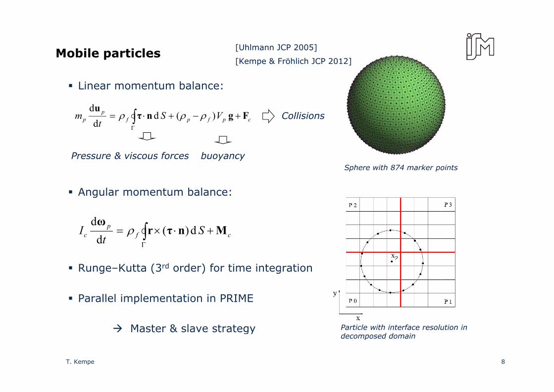
Mobile particles[Uhlmann JCP 2005]

[Kempe & Fröhlich JCP 2012]

Linear momentum balance:

ud

[Kempe & Fröhlich JCP 2012]

cpfpfp

p VSt

m Fgnτu

+−+⋅= ∫Γ

)( dd

dρρρ Collisions

Angular momentum balance:

Pressure & viscous forces buoyancySphere with 874 marker points

g

cfp

c St

I Mnτrω

+⋅×= ∫ d)(d

dρ

Runge–Kutta (3rd order) for time integration

t Γd

Parallel implementation in PRIME

Master & slave strategy Particle with interface resolution in

8

Master & slave strategy Particle with interface resolution in decomposed domain

T. Kempe

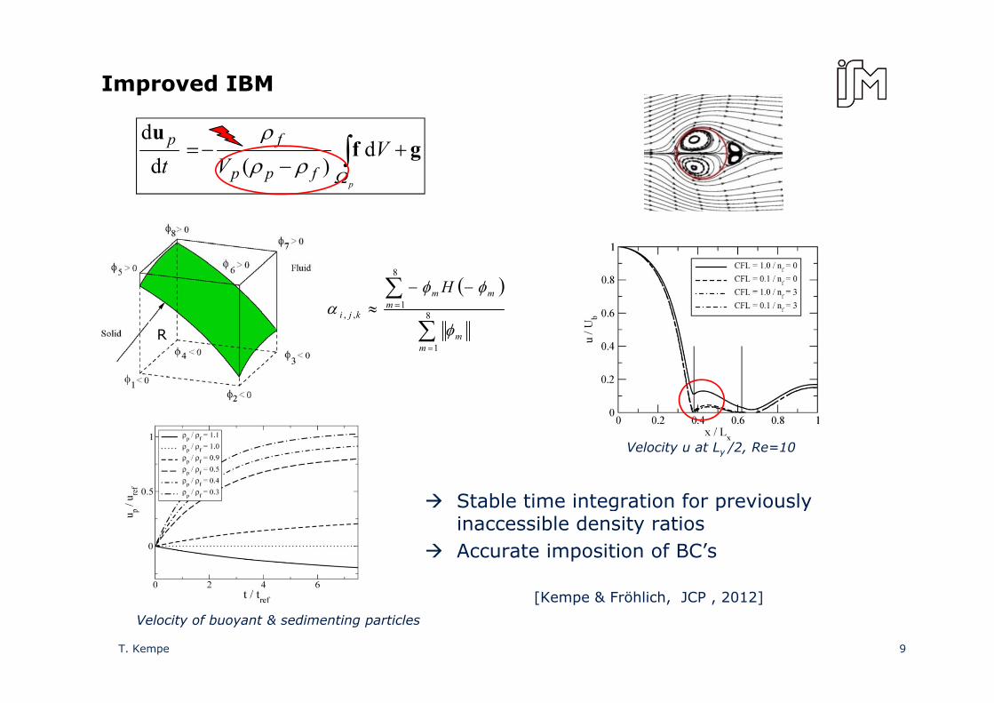
Improved IBM

gfu

+−

−= ∫p

VVt fpp

fp

Ωρρρ

d)(d

d

8

( )

∑

∑

=

=

−−≈ 8

1

8

1,,

mm

mmm

kji

H

φ

φφα

R

Velocity u at Ly /2, Re=10

Stable time integration for previously g p yinaccessible density ratiosAccurate imposition of BC’s

9

Velocity of buoyant & sedimenting particles

[Kempe & Fröhlich, JCP , 2012]

T. Kempe

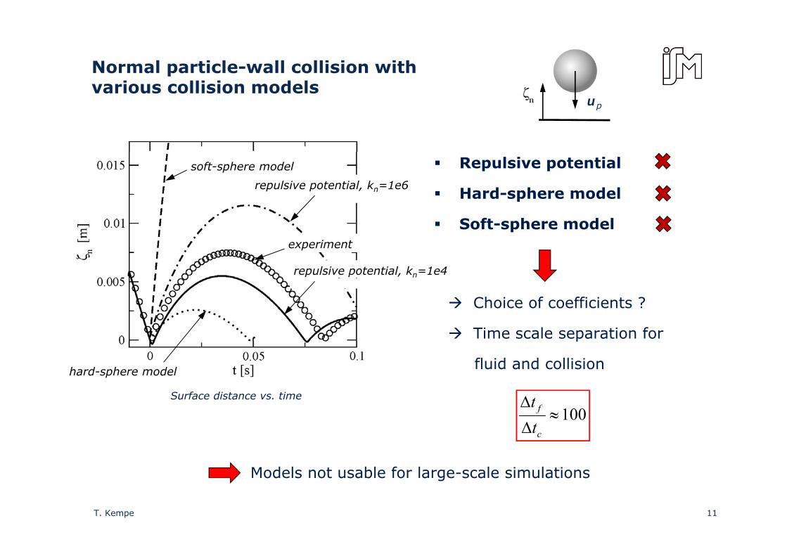
Normal particle-wall collision with various collision modelsvarious collision models

up

soft-sphere model

repulsive potential, kn=1e6

Repulsive potential

Hard-sphere model

experiment

repulsive potential, kn=1e4

Soft-sphere model

Choice of coefficients ?

Time scale separation for

Surface distance vs. time

hard-sphere model

p

fluid and collision

Δt100≈

Δ

Δ

c

f

tt

M d l bl f l l i l i

11

Models not usable for large-scale simulations

T. Kempe

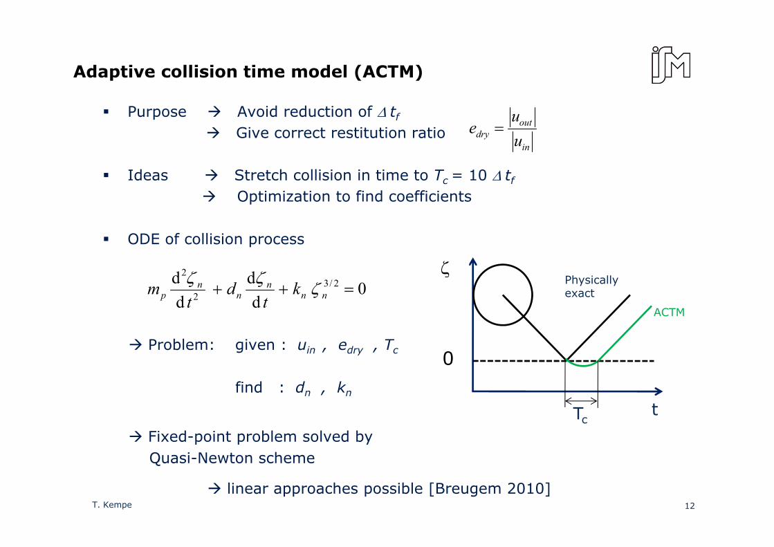
Adaptive collision time model (ACTM)

Purpose Avoid reduction of Δ tf

Give correct restitution ratio in

outdry u

ue =

Ideas Stretch collision in time to Tc = 10 Δ tf

Optimization to find coefficients

in

ODE of collision process

dd2 ζζ ζ0

dd

dd 2/3

2

2

=++ nnn

nn

p kt

dt

m ζζζ Physically exact

ACTM

ζ

Problem: given : uin , edry , Tc

find : dn , kn

rp0

Fixed-point problem solved by Quasi-Newton scheme

tTc

Quasi Newton scheme

12T. Kempe

linear approaches possible [Breugem 2010]

Oblique collisions

Oblique = normal + tangential

Normal ACTM

q

[Joseph 2004]

Normal ACTM

Tangential force model (ATFM)

Consider only sliding and rolling Consider only sliding and rolling

Critical local impact angle

Sliding: Coulomb friction

RSΨ cpinn

cpint

in gg

,

,=Ψ

Sliding: Coulomb friction

Rolling: Compute force such that relative

nfcol

t FF μ=

Rolling: Compute force such that relative

surface velocity is zero 0=cptg

( )( )( ) tF 2

,,,,

2 ppp

intq

intpp

intq

intpppcol

t RmItRuumI

+Δ

+−−=

ωω

13T. Kempe

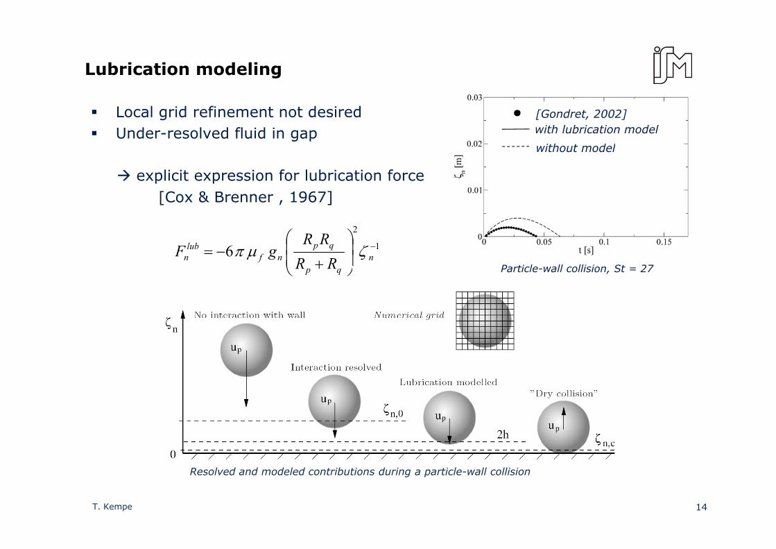
Lubrication modeling

Local grid refinement not desiredUnder-resolved fluid in gap

[Gondret, 2002]with lubrication model

without model

explicit expression for lubrication force [Cox & Brenner , 1967]

without model

1

2

6 −

⎟⎟⎠

⎞⎜⎜⎝

⎛

+−= n

qp

qpnf

lubn RR

RRgF ζμπ

Particle-wall collision, St = 27⎠⎝ qp

14

Resolved and modeled contributions during a particle-wall collision

T. Kempe

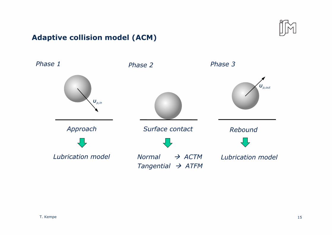
Adaptive collision model (ACM)Adaptive collision model (ACM)

Phase 1 Phase 2 Phase 3Phase 1 Phase 2 Phase 3

Up,out

Up,in

Approach Surface contact Rebound

Lubrication model Normal ACTMTangential ATFM

Lubrication model

15T. Kempe

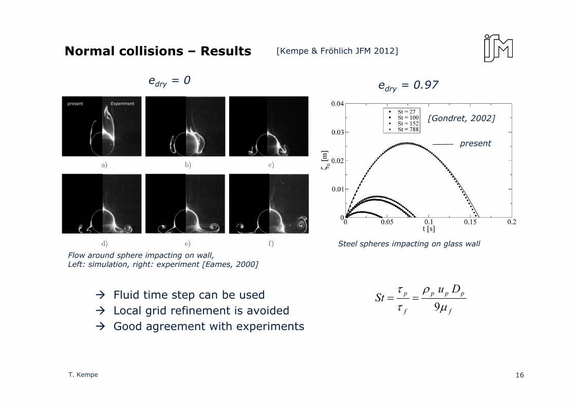
Normal collisions – Results [Kempe & Fröhlich JFM 2012]

edry = 0

present Experiment

edry = 0.97

present

[Gondret, 2002]

Steel spheres impacting on glass wall

Flow around sphere impacting on wall,Left: simulation, right: experiment [Eames, 2000]

Fluid time step can be used pppp DuSt

ρτFluid time step can be usedLocal grid refinement is avoidedGood agreement with experiments

f

ppp

f

pStμτ 9

==

16T. Kempe

Effective angle of impact

Oblique collisions – Results [Kempe & Fröhlich JFM 2012]

Effective angle of impact

Effective angle of rebound

cpinn

cpint

in gg

,

,=Ψ

Effective angle of rebound

cpinn

cpoutt

out gg

,

,=Ψcp

outtgcp

inng ,cp

intg ,

Compared with experiment [Joseph, 2004]

Glass spheres, rough, μ f = 0.15Steel spheres, smooth, μ f = 0.01

outtg ,

Glass spheres, rough, μ f 0.15ΨRS = 0.95

present

p μ f ΨRS = 0.25

sliding

ΨRS

rolling

Ψ

17T. Kempe

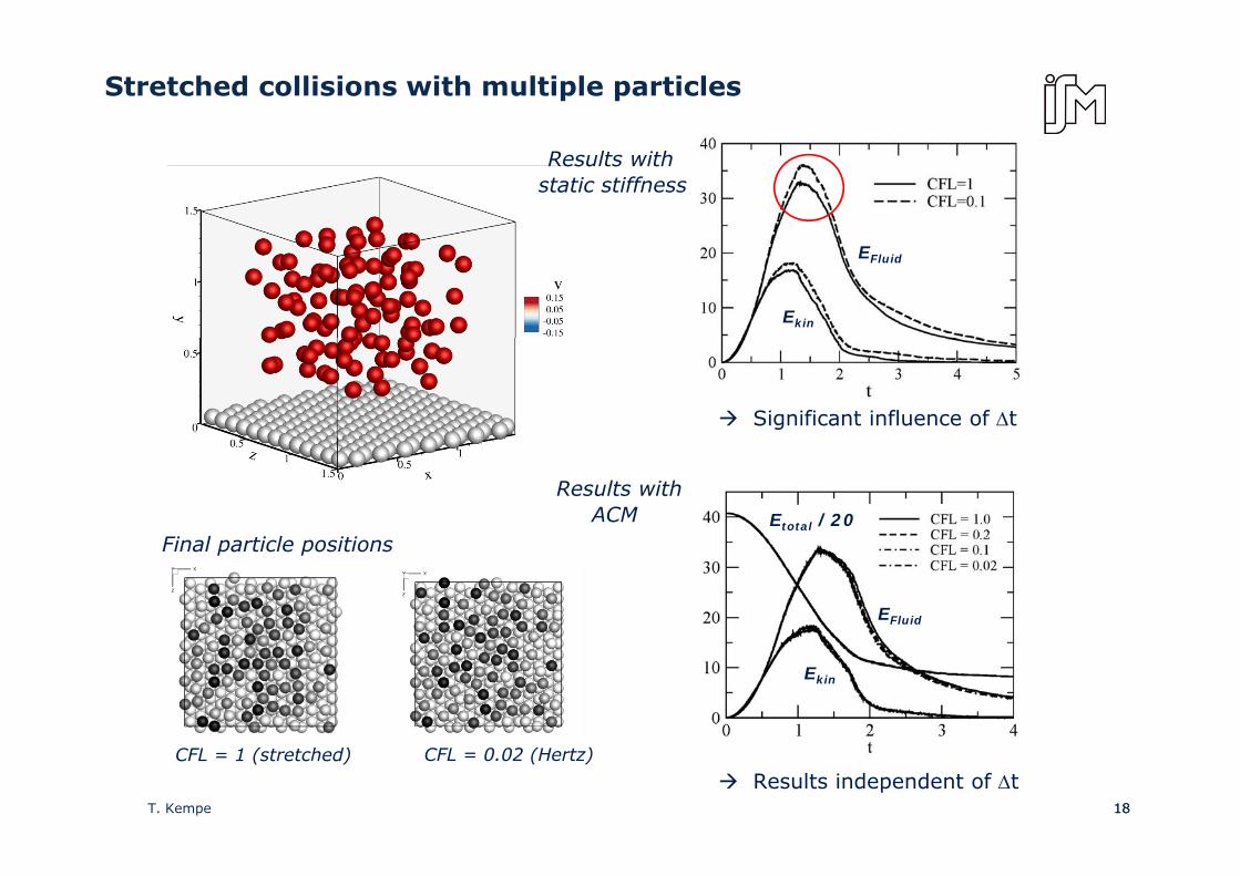
Stretched collisions with multiple particles

Results with static stiffness

EFluid

Ekin

Significant influence of Δt

Results with ACM

Fi l ti l iti Etotal /20

Final particle positions

EFluid

Ekin

1818T. Kempe

CFL = 1 (stretched) CFL = 0.02 (Hertz)

Results independent of Δt

3D interface resolved

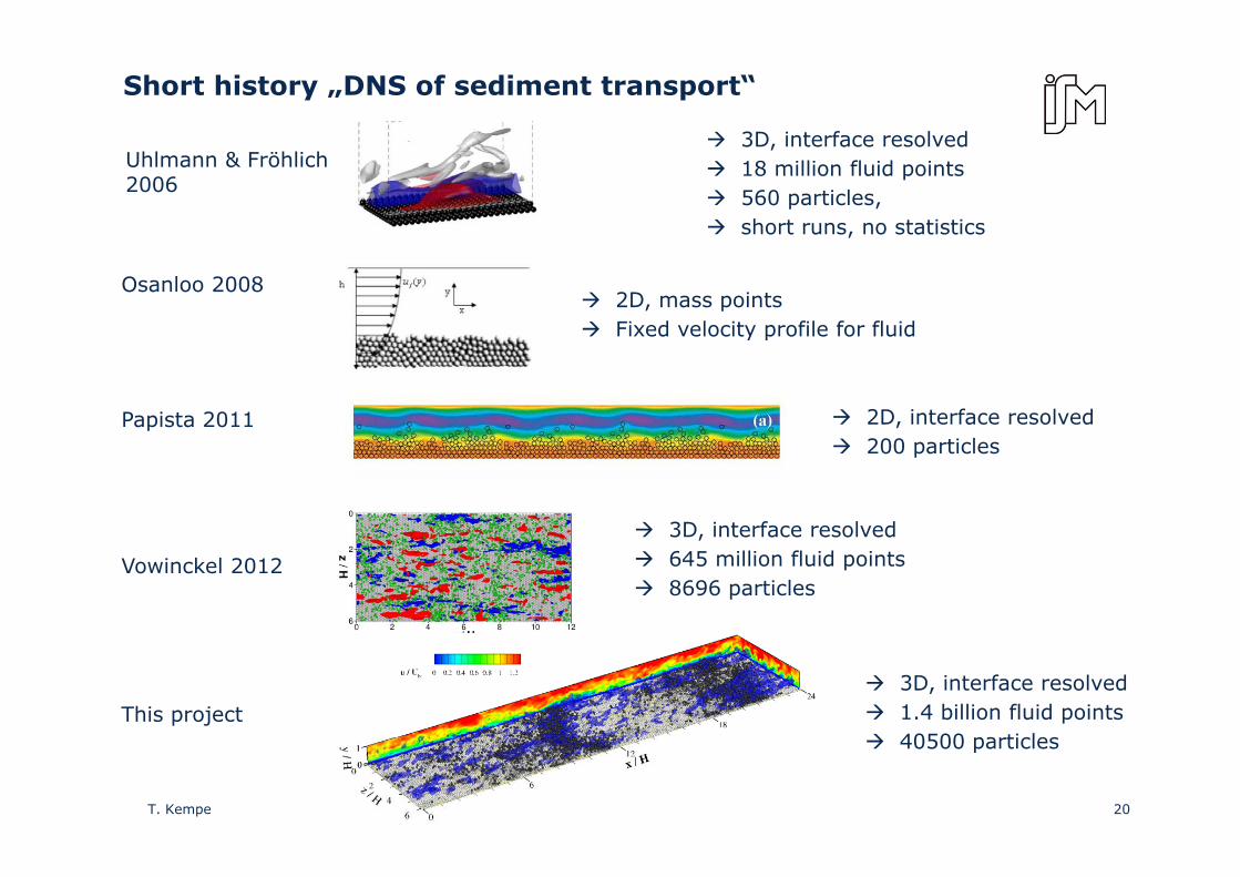
Short history „DNS of sediment transport“

Uhlmann & Fröhlich 2006

3D, interface resolved18 million fluid points560 particles, short runs, no statistics

Osanloo 20082D, mass pointsFixed velocity profile for fluid

Papista 2011

y p

2D, interface resolved200 i l200 particles

3D, interface resolved

Vowinckel 2012

,645 million fluid points8696 particles

This project

3D, interface resolved1.4 billion fluid points40500 pa ticles40500 particles

20T. Kempe

Computational Setup

H/D Lx/H Lz/H Reb Reτ D+

9 24 6 2941 193 21

Two layers of particles:

• Fixed bed: single layer of hexagonal packing

• Sediment bed on top

Free slipp

No slip

Periodic in x- and z- direction 21T. Kempe

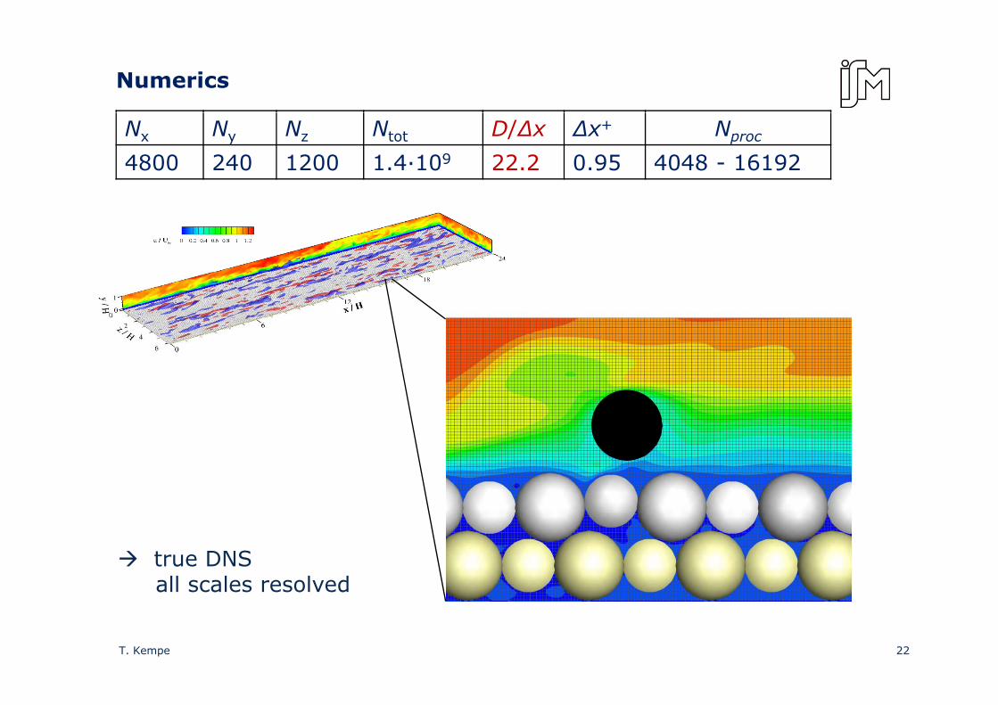
Numerics

Nx Ny Nz Ntot D/Δx Δx+ Nproc

4800 240 1200 1.4·109 22.2 0.95 4048 - 16192

true DNS all scales resolved

22T. Kempe

Computational Setup

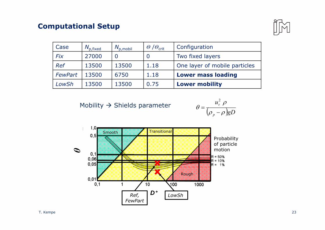
Case Np,fixed Np,mobil Θ /Θcrit Configuration

Fix 27000 0 0 Two fixed layers

Ref 13500 13500 1.18 One layer of mobile particles

FewPart 13500 6750 1.18 Lower mass loading

LowSh 13500 13500 0.75 Lower mobility

( )gDu

p ρρρ

θ τ

−=

2

Mobility Shields parameter( )gp ρρ

Probability

TransitionalSmooth

θ

of particlemotion

D+f

Rough

DRef,FewPart

LowSh

23T. Kempe

Case Ref Θ /Θcrit = 1.18 [Vowinckel et al. ICMF 2013]

Spanwise oriented dunes

Contour Iso-surfaces of fluctuations Particleu / Uu / Ub

u' / Ub = -0.3' / U 0 3

up / uτ ≥ 4up / uτ< 4fixedu' / Ub = 0.30

24T. Kempe

Case Ref Θ /Θcrit = 1.18

mean fluid velocity fluctuations <u’ u’>

0.8

1

Fix

0.8

1

mean fluid velocity 

0.8

1y

/ H

-0.2

0

0.2

0.4

0.6

0.8 FixRefFewPartLowSh

y / H

0.2

0.4

0.6

y / H

0.2

0.4

0.6

 / Ub

0 0.5 1-0.2

Mobile or restingFixed bed

 / U0 0.5 1

-0.2

0

0.2

<u’u’> / U20 0.02 0.04 0.06-0.2

0

0.2

 / Ub<u’u’> / Ub

higher intrusion, larger resistance, more turbulence25T. Kempe

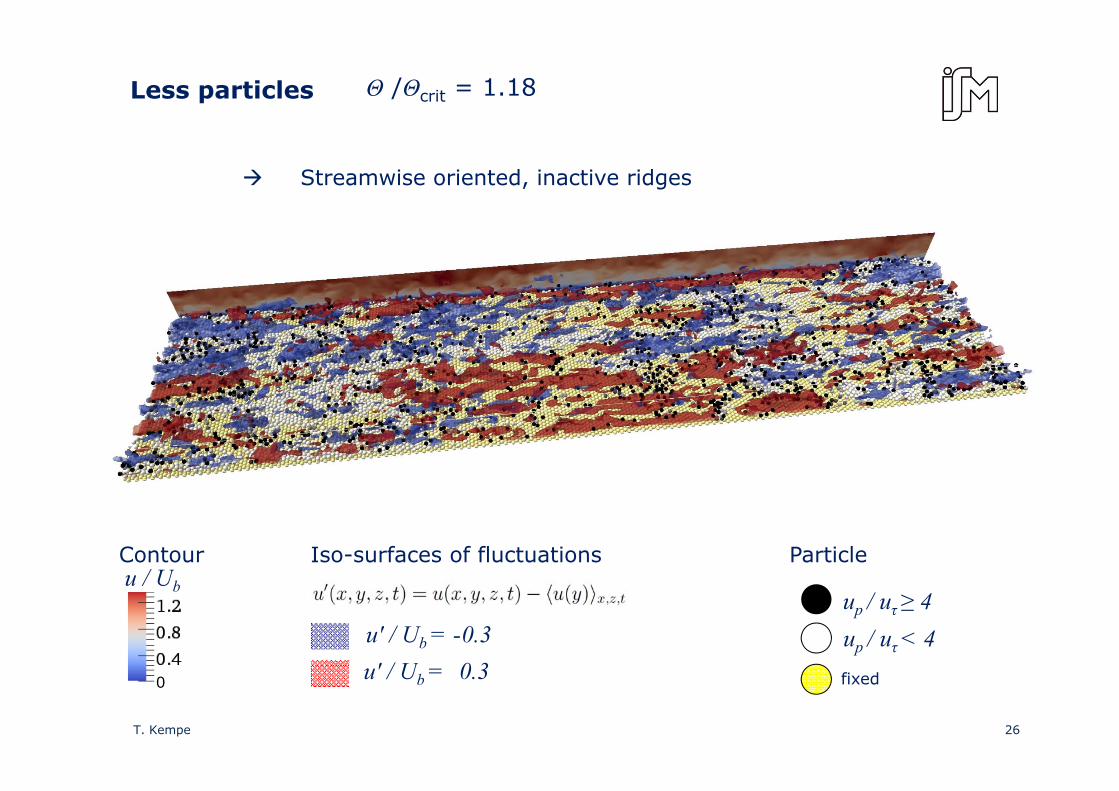
Less particles Θ /Θcrit = 1.18

Streamwise oriented, inactive ridges

Contour Iso-surfaces of fluctuations Particleu / U

u' / Ub = -0.3' / U 0 3

up / uτ ≥ 4up / uτ< 4

u / Ub

fixedu' / Ub = 0.30

26T. Kempe

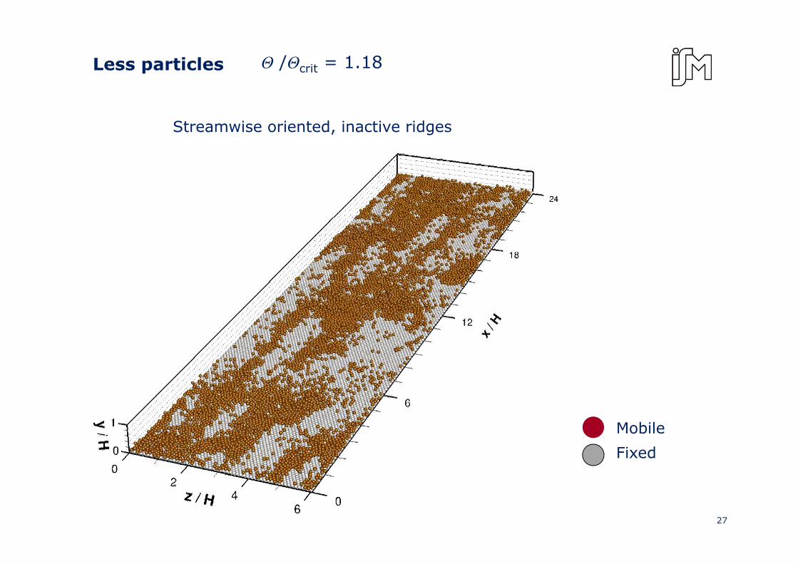
Less particles Θ /Θcrit = 1.18

Streamwise oriented, inactive ridges

Mobile

Fixed

27T. Kempe

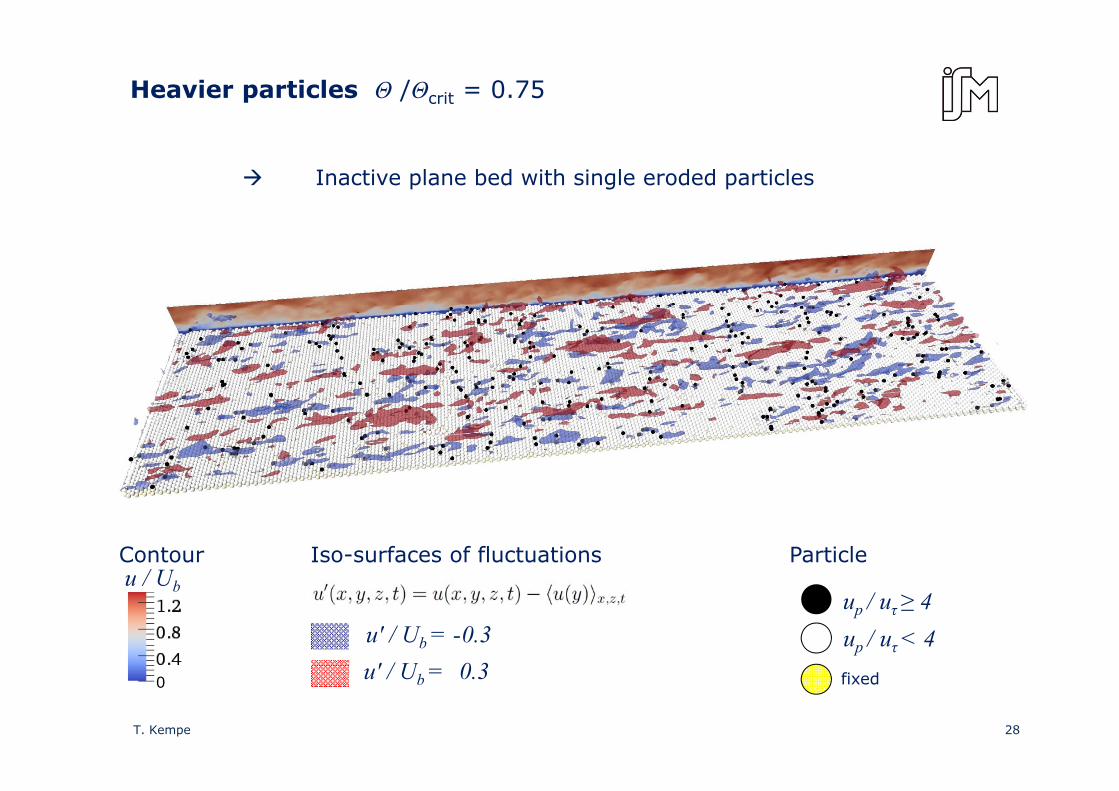
Heavier particles Θ /Θcrit = 0.75

Inactive plane bed with single eroded particles

Contour Iso-surfaces of fluctuations Particleu / U

u' / Ub = -0.3' / U 0 3

up / uτ ≥ 4up / uτ< 4

u / Ub

fixedu' / Ub = 0.30

28T. Kempe

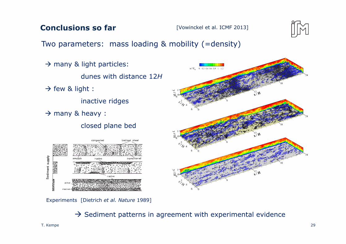
Conclusions so far [Vowinckel et al. ICMF 2013]

many & light particles:

Two parameters: mass loading & mobility (=density)

y g p

dunes with distance 12H

few & light :

inactive ridges

many & heavy :

closed plane bed

Experiments [Dietrich et al. Nature 1989]

Sediment patterns in agreement with experimental evidence29T. Kempe

Bubble shape depends on regime

Reynolds number

[Clift et al. 1978]

number

νeqpdu

=Reν

ρρ 2dg

Eötvös numberσρρ eqfp dg

Eo−

=

31T. Kempe

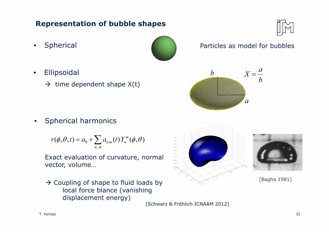
Representation of bubble shapes

• Spherical Particles as model for bubbles

• Ellipsoidal

time dependent shape X(t)baX =b

a

• Spherical harmonics

∑+= mnmn Ytaatr 0 ),()(),,( θφθφ

Exact evaluation of curvature, normal vector, volume…

∑mn

nmn,

0 ),()(),,( φφ

[Bagha 1981]Coupling of shape to fluid loads by local force blance (vanishing displacement energy)

32T. Kempe

[Schwarz & Fröhlich ICNAAM 2012]

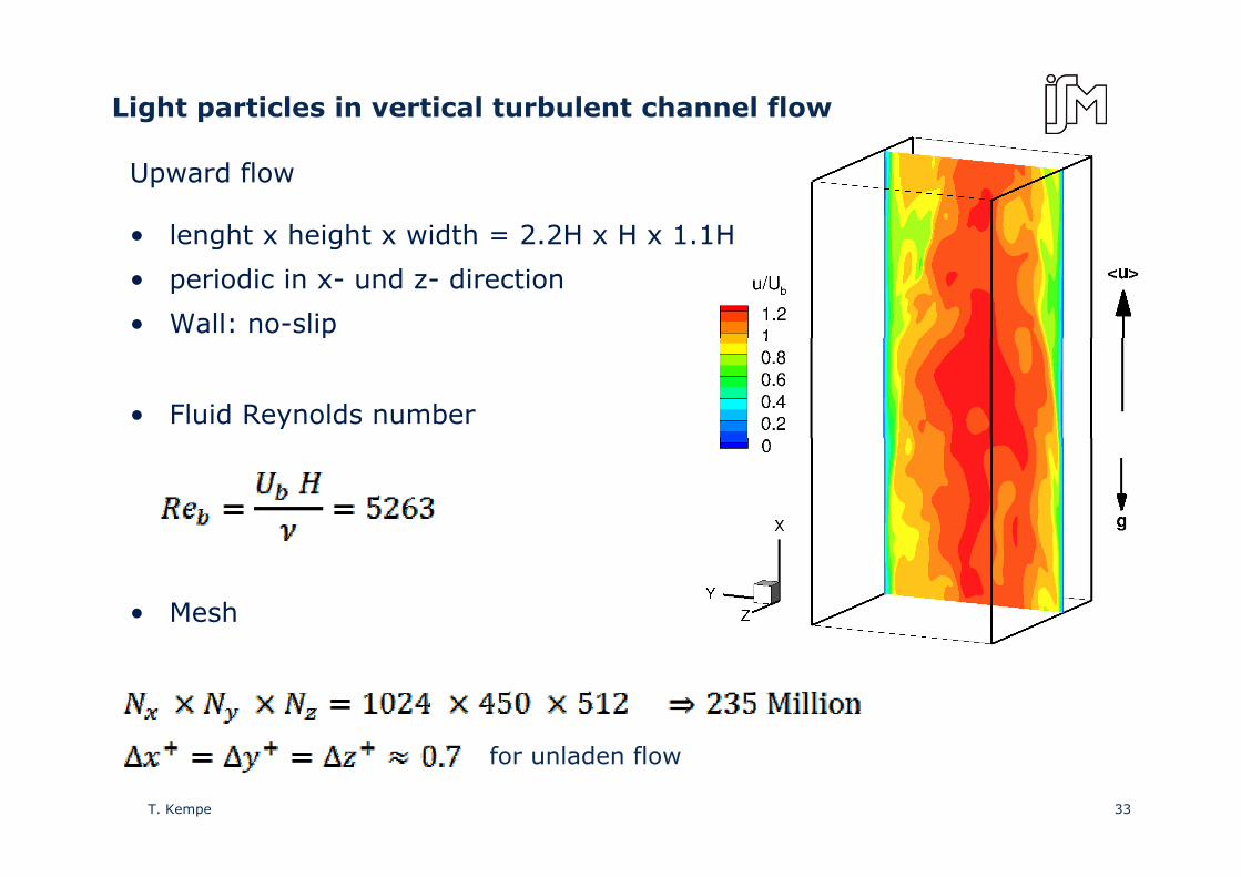
Light particles in vertical turbulent channel flow

Upward flow

• lenght x height x width = 2 2H x H x 1 1H• lenght x height x width 2.2H x H x 1.1H

• periodic in x- und z- direction

• Wall: no-slip

• Fluid Reynolds number

• Mesh

for unladen flow

33T. Kempe

Particle parameters

Fixed shape:

oblate ellipsoid

0 001ρp

Density ratio: 0.001ρf

Density ratio:

Np Deq/H Deq/∆ a/b Void fr. Rep

740 0.05172 ~24 2 ~ 2 % ~214

34T. Kempe

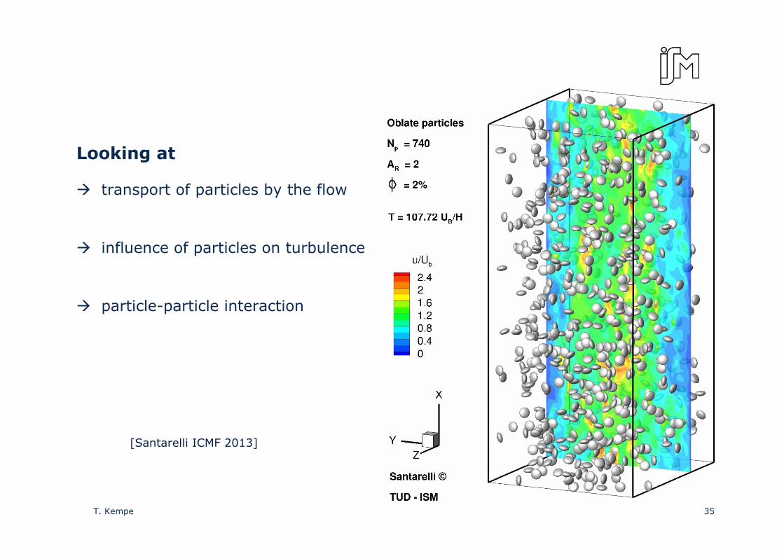
Looking atLooking at

transport of particles by the flow

influence of particles on turbulence

particle-particle interaction

[Santarelli ICMF 2013]

35T. Kempe

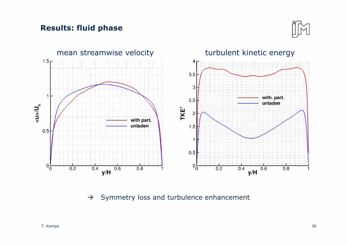
Results: fluid phase

mean streamwise velocity turbulent kinetic energy

Symmetry loss and turbulence enhancement

36T. Kempe

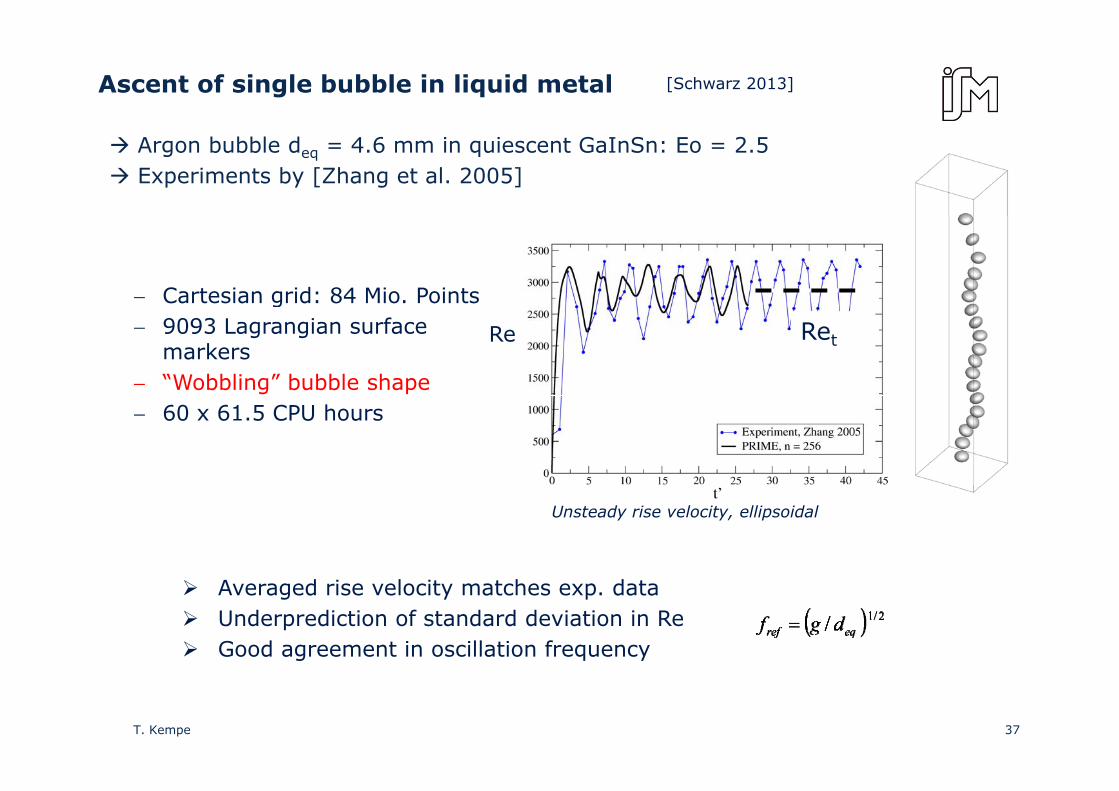
Ascent of single bubble in liquid metal [Schwarz 2013]

Argon bubble deq = 4.6 mm in quiescent GaInSn: Eo = 2.5Experiments by [Zhang et al. 2005]

− Cartesian grid: 84 Mio. Pointsg− 9093 Lagrangian surface

markers− “Wobbling” bubble shape

Re Ret

− 60 x 61.5 CPU hours

PRI• Comparison

Unsteady rise velocity, ellipsoidal

0.270.28f / 245369σRe

2871

2879

MEAveraged rise velocity matches exp. dataUnderprediction of standard deviation in ReGood agreement in oscillation frequency0.27

60.28

0f / fref

245369σRe[Schwarz, 2011, 2013]

37T. Kempe

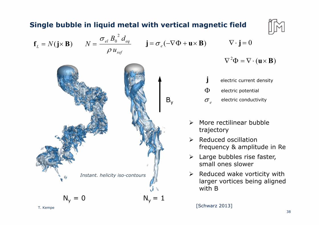
Single bubble in liquid metal with vertical magnetic field

dB 2

ref

eqel

udB

Nρ

σ 20=)( Bjf ×= NL )( Buj ×+Φ−∇= eσ 0=⋅∇ j

)(2 Bu×⋅∇=Φ∇

electric current density jj

)( Bu×⋅∇=Φ∇

By

By

electric potentialjelectric conductivity jeσ

Φ

More rectilinear bubbletrajectory

R d d ill tiReduced oscillationfrequency & amplitude in Re

Large bubbles rise faster, small ones slower

Ny = 0 Ny = 1

small ones slower

Reduced wake vorticity with larger vortices being alignedwith B

Instant. helicity iso-contours

38

with B

Ny = 0 Ny = 1T. Kempe [Schwarz 2013]

Thank you for your attention.

Feedback and questions ? q

Bubble Coalescence

13:10 – 13:30

S Sch a S Tschisgale and J F öhlich S. Schwarz, S. Tschisgale and J. Fröhlich

“Bubble coalescence model for phase-resolving simulations using an Immersed Boundary Method”

39T. Kempe

application of the immersed boundary method to particle...

Documents