Applications of Multi-Layer PerceptronsNeural Computation : Lecture 11

© John A. Bullinaria, 2015

1. Types of Feed-Forward Neural Network Applications

2. Brain ModellingWhat Needs Modelling?Development, Adult Performance, NeuropsychologyAnalysis of Hidden Unit Representations

3. Real World ApplicationsData Compression - PCATime Series PredictionCharacter Recognition and What-WhereAutonomous Driving - ALVINN

L11-2

Types of Feed-Forward Neural Network ApplicationsWe have already noted that there are two basic goals for neural network research:

Brain modelling : The scientific goal of building models of how real brains work.This can potentially help us understand the nature of human intelligence, formulatebetter teaching strategies, or better remedial actions for brain damaged patients.

Artificial System Building : The engineering goal of building efficient systems forreal world applications. This may make machines more powerful, relieve humansof tedious tasks, and may even improve upon human performance.

These should not be thought of as competing goals. We often use exactly the sameneural networks and techniques for both. Frequently progress is made when the twoapproaches are allowed to feed into each other. There are fundamental differencesthough, e.g. the need for biological plausibility in brain modelling, and the need forcomputational efficiency in artificial system building. Simple feed-forward neuralnetworks, such as MLPs, are surprisingly effective for both.

L11-3

Brain Modelling – What Needs Modelling?

It makes sense to use all available information to constrain our theories/models of realbrain processes. This involves gathering as much empirical evidence about brains as wecan (e.g., by carrying out psychological experiments) and comparing it with the models.

The comparison between brains and models fall into three broad categories:

Development : Comparisons of children’s development with that of our models – thiswill generally involve both maturation and learning.

Adult Performance : Comparisons of our mature trained models with normal adultperformance – exactly what is compared depends on what we are modelling.

Brain Damage / Neuropsychological Deficits : Often performance deficits, e.g. due tobrain damage, tell us more about normal brain operation than normal performance.

We shall consider these issues for a particularly simple and familiar task – “readingaloud” or “text to phoneme conversion”. Similar considerations will apply to a widerange of psychological tasks that can be reduced to forms of input output mappings.

L11-4

The NETtalk Model of Reading

The NETtalk model of Sejnowski & Rosenberg (1987) is a basically a MLP whichgenerates output phonemes corresponding to the letter in middle of an input window:

output - phonemes

hidden layer

input - letters

(nhidden)

(nchar • nletters)

(nphonemes)

The network can also be set up to figure out the letter-phoneme alignments for itself byassuming the alignment that best fits in with its expectations (Bullinaria, 1997).

We’ll look at the results from a typical series of simulations. The network training dataconsisted of all 2998 English monosyllabic words, and the testing data was a standardset of 166 made up pronounceable non-words. It was trained using a standard learningalgorithm (back-propagation with momentum) with 300 hidden units.

L11-5

Development ≈ Network Learning

If neural network models are to provide a good account of what happens in real brains,we should expect their learning process to be similar to the development in children.

10001001010

20

40

60

80

100

Training DataRegular WordsException WordsNon-Words

Epoch

Perc

enta

ges

Cor

rect

The networks find regular words (e.g. ‘bat’) easier to learn that exception words (e.g.‘yacht’) in the same way that children do. It also learns human-like generalization.

L11-6

Developmental Problems ≈ Restricted Network Learning

Many dyslexic children exhibit a dissociation (performance difference) between regularand irregular word reading. There are many ways this can arise in network models:

10001001010

20

40

60

80

100

RegularExceptionNon-words

RegularExceptionNon-words

Epoch

Perc

enta

ge

Cor

rect

15 HU

No SPO

1. Limitation on computational resources (e.g., only 15 hidden units)2. Sub-optimal learning algorithm (e.g., SSE cost function and no SPO)3. Simple delay in learning (e.g., due to low learning rate η)

L11-7

Adult Performance ≈ Trained Network Performance

Having succeeded in building accurate models of children’s development, one might thinkthat our adult models (fully trained neural networks) require little further testing. In fact,largely due to better availability and reliability of the empirical data, there are a range ofadult performance measures that prove useful for constraining our models, such as:

Accuracy – basic task performance levels, e.g. how well are particular aspects of alanguage spoken/understood, or how well can we estimate a distance?

Generalization – e.g. how well can we pronounce words we have never seen before(vowm fi gowpiet?), or recognise an object from an unseen direction?

Reaction Times – response speeds and their differences, e.g. can we recognise oneword type faster than another, or respond to one colour faster than another?

Priming – e.g. if asked whether dog and cat are real words, one tends to say yes to catfaster than if asked about dot and cat (this is lexical decision priming).

Speed-Accuracy Trade-off – across a wide range of tasks your accuracy tends toreduce as you try to speed up your response, and vice-versa.

Different performance measures will be appropriate to test different models.

L11-8

Brain Damage ≈ Network Damage

Neural network models have natural analogues of brain damage – removal of sub-sets ofneurons and connections, adding noise to the weights, scaling the activation functions. Ifwe damage the reading model, the regular items are more robust than the irregulars:

16141210864200

20

40

60

80

100

Regular Words Exception WordsRegular Non-Words

Degree of Damage

Perc

enta

ge

Cor

rect

These neural network deficits are the same as seen in human acquired Surface Dyslexia.

L11-9

Analysing the Internal Representations

3020100-10-20-30-30

-20

-10

0

10

20

30

/i/ projection

/I/

proj

ecti

on

limb - /lim/grind - /grind/live - /liv/spilt - /spilt/wind - /wind/pith - /piT/

pint - /pInt/wind - /wInd/wild - /wIld/rind - /rInd/hive - /hIv/bind - /bInd/

been - /bin/cyst - /sist/sieve - /siv/

hinge - /hindZ/

ire -

/Ir/

heig

ht -

/hI

t/

stei

n -

/stI

n/

guy

- /g

I/fie

ld -

/fIl

d/

buy

- /b

I/

chick - /Cik/nicks - /niks/

/I/ WORDS

/i/ WORDS

One can look at the represent-ations the neural network learnson its hidden layer. The graphshows the activation sub-spacecorresponding to the distinctionbetween long and short ‘i’sounds, i.e. the ‘i’ in ‘pint’versus the ‘i’ in ‘pink’. Theirregular words are closest to theborder line. So, after networkdamage, it is these that cross theborder line and produce errorsfirst. Moreover, the errors willmostly be regularizations. Thisis exactly the same as is foundwith human surface dyslexics.

L11-10

Real World Applications

The real world applications of feed-forward neural networks are endless. Some wellknown ones that get mentioned in the recommended text books are:

1. Airline Marketing Tactician (Beale & Jackson, Sect. 4.13.2)2. Backgammon (Hertz et al., Sect. 6.3)3. Data Compression – PCA (Hertz et al., Sect. 6.3; Bishop, Sect. 8.6) •4. Driving – ALVINN (Hertz et al., Sect. 6.3) •5. ECG Noise Filtering (Beale & Jackson, Sect. 4.13.3)6. Financial Prediction (Beale & Jackson, Sect. 4.13.3; Gurney, Sect. 6.11.2) •7. Hand-written Character Recognition (Hertz et al., Sect. 6.3; Fausett, Sect. 7.4) •8. Pattern Recognition/Computer Vision (Beale & Jackson, Sect. 4.13.5) •9. Protein Secondary Structure (Hertz et al., Sect. 6.3)10. Psychiatric Patient Length of Stay (Gurney, Sect. 6.11.1)11. Sonar Target Recognition (Hertz et al., Sect. 6.3)12. Speech Recognition (Hertz et al., Sect. 6.3)13. Text to Phoneme Mapping (Beale & Jackson, Sect. 4.13.1; Bullinaria, 2011) •

L11-11

Data Compression - PCA

An auto-associator network is one that has the same outputs as inputs. If in this casewe make the number of hidden units M smaller than the number of inputs/outputs N, wewill have clearly compressed the data from N dimensions down to M dimensions.

Such data compression networks have many applications where data transmission ratesor memory requirements need optimising, such as in image compression. They clearlywork by removing the redundancy that exists in the data. It can be shown that thehidden unit representation spans the M principal components of the original Ndimensional data, so standard PCA considerations apply (Bourland & Kamp, 1988).

N units

N units

M units

Input Patterns

Input Patterns

Compressed Representations

L11-12

Time Series Prediction

Neural networks have been applied to numerous situations where time series predictionis required – predicting weather, climate, stocks and share prices, currency exchangerates, airline passengers, etc. We can turn the temporal problem into a simple input-output mapping by taking the time series data x(t) at k time-slices t, t–1, t–2, …, t–k+1as the inputs, and the output is the prediction for x(t+1).

Such networks can be extended in many ways, e.g. additional inputs for information otherthan the series x(t), outputs for further time steps into the future, feeding the outputs backthrough the network to predict further into the future (Weigend & Gershenfeld, 1994).

x(t+1)

x(t–2) x(t–1) x(t)x(t–k+1) • • •

L11-13

Hand-written Character Recognition

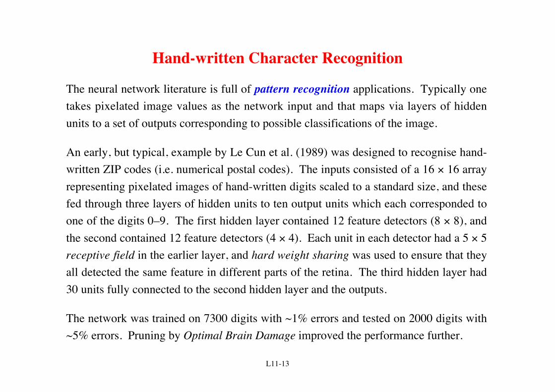
The neural network literature is full of pattern recognition applications. Typically onetakes pixelated image values as the network input and that maps via layers of hiddenunits to a set of outputs corresponding to possible classifications of the image.

An early, but typical, example by Le Cun et al. (1989) was designed to recognise hand-written ZIP codes (i.e. numerical postal codes). The inputs consisted of a 16 × 16 arrayrepresenting pixelated images of hand-written digits scaled to a standard size, and thesefed through three layers of hidden units to ten output units which each corresponded toone of the digits 0–9. The first hidden layer contained 12 feature detectors (8 × 8), andthe second contained 12 feature detectors (4 × 4). Each unit in each detector had a 5 × 5receptive field in the earlier layer, and hard weight sharing was used to ensure that theyall detected the same feature in different parts of the retina. The third hidden layer had30 units fully connected to the second hidden layer and the outputs.

The network was trained on 7300 digits with ~1% errors and tested on 2000 digits with~5% errors. Pruning by Optimal Brain Damage improved the performance further.

L11-14

Zip-Code Neural Network Architecture

From: Introduction to the Theory ofNeural Computation, Hertz, Krogh& Palmer, Addison-Wesley, 1991.

L11-15

Processing “What” and “Where” Together

General pattern recognition requires the determination of “What” and “Where” at thesame time, from the same pixelated images. It is not obvious if this is best done usingone big network for both tasks, or separate networks. Experiments to test this have beencarried out on simple 5 × 5 images on a network with parameterized architecture:

9 "what" 9 "where"

5 × 5 retina

Nhid1 Nhid2Nhid12

Input Layer

Hidden layer

Output Layer

The conclusion depends on precisely what learning algorithm is used and how well theneurophysiological constraints (e.g., wiring volumes) are modelled (Bullinaria, 2007).

L11-16

Simplified “What-Where” Training Data“What” = Nine 3 × 3 Patterns “Where” = Nine Positions in 5 × 5 Retina

9 × 9 = 81 Training Patterns in total

e.g. 01110 00100 00100 00000 00000 100000000 010000000Input (5 × 5 = 25 units) What (9 units) Where (9 units)

L11-17

Autonomous Driving – ALVINN

Pomerleau (1989) constructed a neural network controller ALVINN for driving a car ona winding road. The inputs were a 30 × 32 pixel image from a video camera, and an8 × 32 image from a range finder. These were fed into a hidden layer of 29 units, andfrom there to a line of 45 output units corresponding to the direction to drive.

The network was originally trained using back-propagation on 1200 simulated roadimages. After about 40 epochs the network could drive at about 5mph – the speed beinglimited by the speed of the computer that the neural network was running on.

In a later study the network learnt by watching how a human steered, and by usingadditional views of what the road would look like at positions slightly off course. Afterabout three minutes of training, ALVINN was able to take over and continue to drive.ALVINN has successfully driven at speeds up to 70mph and for distances of over 90miles on a public highway north of Pittsburgh. (Apparently, actually being inside thevehicle during the neural network’s test drive was a big incentive for the researchers todevelop a good neural network!) Recent versions have been even more impressive.

L11-18

ALVINN Architecture

From: Advances in Neural InformationProcessing Systems 1, D.S. Touretzky(Ed.), Morgan Kaufmann, 1989.

L11-19

References / Advanced Reading List

1. Bourland, H. & Kamp, Y. (1988). Auto-association by Multilayer Perceptrons andSingular Values Decomposition. Biological Cybernetics, 59, 291-294.

2. Bullinaria, J.A. (1997). Modelling Reading, Spelling and Past Tense Learning withArtificial Neural Networks. Brain and Language, 59, 236-266.

3. Bullinaria, J.A. (2007). Understanding the Emergence of Modularity in Neural Systems.Cognitive Science, 31, 673-695.

4. Bullinaria, J.A. (2011). Text to Phoneme Alignment and Mapping for SpeechTechnology: A Neural Networks Approach. In: Proceedings of the International JointConference on Neural Networks (IJCNN 2011), 625-632. IEEE.

5. Le Cun, Y. et al. (1989). Back-propagation Applied to Handwritten Zip CodeRecognition. Neural Computation, 1, 541-551.

6. Pomerleau, D.A. (1989). ALVINN: An Autonomous Land Vehicle in a Neural Network.In: D.S. Touretzky (ed.), Advances in Neural Information Processing Systems I, 305-313.Morgan Kaufmann.

7. Sejnowski, T.J. & Rosenberg, C.R. (1987). Parallel Networks that Learn to PronounceEnglish Text. Complex Systems, 1, 145-168.

8. Weigend, A.S. & Gershenfeld, N.A. (1994). Time Series Prediction: Forecasting theFuture and Understanding the Past. Addison-Wesley.

L11-20

Overview and Reading

1. We began by recalling the distinction between using neural networks forbrain modelling and for artificial system building.

2. Then we looked at the main issues in brain modelling (development, adultperformance, and neuropsychology) with reference to a reading model,and saw how one can better understand the operation of particular neuralnetworks by looking at the patterns of activation on their hidden layer.

3. We ended by looking at a selection of real world applications, with fivestudied in particular detail: data compression, times series prediction,character recognition, the what-where task, and autonomous driving.

Reading

1. Hertz, Krogh & Palmer: Section 6.32. Gurney: Section 6.113. Beale & Jackson: Section 4.134. Ham & Kostanic: Chapters 6 to 10