APPLICATIONS OF RESISTIVITY METHODS

AND

MICRO-EARTHQUAKE MONITORING IN GEOTHERMAL EXPLORATION

MULYADI*

UNU Geothermal Training Programme

National Energy Authority

Grens8.svegur 9,

108 Reykjavik

ICELAND

*Permanent address:

PERTAMINA

GEOTHERMAL DIVISION

Jalan : Kramat Raya 59,

Jakarta Pusat,

Jakarta,

INDONESIA.

ABSTRACT

This report contains two chapters, describing resistivity

methods and micro-earthquake monitoring applied to explore

geothermal resources.

Four resistivity methods with their applications in geothermal

areas, i.e. Schlumberger, Head-on, and Wenner, Dipole-dipole

used for exploration at Broadlands (New Zealand) and Hvitbolar

(Iceland), respectively, are observed. The combinations of

resistivity data of Schlumberger and Head-on may probably be

useful to construct 2-D resistivity model.

The hypocenters of micro-earthquakes monitored in the period

of six months at Lahendong, Indonesia, were originally calculated

by using single layer velocity model. While in this study,

they were recalculated by usina multiple layer velocity

model. The events significantly cluster outside the caldera

rim and only a few are located inside the caldera at relatively

shallow depth. This phenomenon may be due to fracturin~

along the contact area between hot fluids and cool rocks, or,

hot rocks and meteoric water at depth. The distribution of

hypocenters could also be the result of the combination of

overburden pressure and temperature. Hence, the number of

events reaches a maximum at depths of about 2-3 k. reflecting

either the depths of the highest rate of volumetric contraction

or high heat flow in the area.

TABLB OF CONTENTS

ABSTRACT

INTRODUCTION

PART ONE ..

1. REVIEW OF RESISTIVITY METHODS 1 . 1 . Basic Theory of Resistivity 1. 2 . Solving Rising Problems

1.2.1. Topo,raphy 1 . 2.2 . Inhomogeneity .... 1 . 2.3. Practical field operation 1 . 2.4 . Data processing .. ...

1.3. Resistivity Array Method 1 . 3.1. Schluaberger and Head-On

1.3.1 . 1. Schlumberger . . 1.3 . 1 . 2 . Head-On ....

1 . 3 . 2. Wenner And Dipole-Dipole 1.3 . 2.1. Wenner . .. • 1.3.2.2. Dipole-Dipole

2. WENNER AND DIPOLE-DIPOLE METHODS

3 . SCHLUMBERGER AND HEAD-ON METHODS 3 . 1. Geological setti ng . . . 3 . 2. Review of the Geothermal Area 3 . 3. Resistivity Modelling

4 . DISCUSSION

5 . CONCLUSIONS

PART TWO • • •

6 . RELOCATING HYPOCENTERS OF MICRO-EARTHQUAKES 6.1. INTRODUCTION . . . .. . . . . ... . 6 . 2. REVIEW OF EARTHQUAKE MONITORING • • • 6.3. GEOLOGICAL AND GEOPHYSICAL BACKGROUND

6.3 . 1. Geological Setting 6 . 3.2. Geophysical Exploration .. . .

6 . 4 . EQUIPMENT AND DATA PROCESSING •• . . 6 . 4.1 . Equipment . . . . . . . . . . . 6.4 . 2. Locating The Micro-Earthquakes 6.4.3. Magnitude

6 . 5. RESULTS 6.6 . DISCUSSIONS 6.7. CONCLUSIONS 6 . 8 . SUGGESTION

ACKNOWLEDGEMENTS

REFERENCES . . .

2

6

7

7 7 8 8 8 9 9

11 11 11 12 12 12 13

14

15 15 15 16

18

20

21

21 21 21 22 22 23 23 23 24 25 25 26 27 28

29

30

List of Tables

Table 1 . Attempted crustal velocity models used to calculate the hypocenters of micro-earthquakes monitored during January -June, 1985, at Lahendong geothermal area, Indonesia. 34

Table 2. Shows coordinates of the seismometer locations. 34

Figure 1. The

Figure 2. The

Figure 3. The

Figure 4. The

a)

d)

List of Figures

electrode array of Schlumberger.

electrode array of Head- on.

electrode array of Wenner.

electrode array of dipole-dipole,

azimuthal, b) radial, c) paral l e l,

perpendicular.

and

35

35

35

35

Figure 5. Geothermal field boundary, Broadlands, New Zealand.

a) by appl y ing Wenner method with a=550m, and

b) dipole-dipole method. 36

Figure 6. 2-D resistivity model of B-W section, Hvitholar

geothermal area, constructed from :

a) Head-on and b) Schlumberger methods,

(Arnason et al ., 1984).

Figure 7. 2-D resistivity model of B-W section, Hvitholar

geothermal area, constructed from the combination

of the Schlumberger and Head-on method.

Figure 8a. Contour of observed apparent resistivities

(Schlumberger), E-W section, Hvitholar,

Iceland.

37

38

39

Figure 8b. Contour of apparent resistivities (Schluaberger),

calculated by using 2-D resistivity model of E-W

Figure 9

section, Hvitholar, Iceland. 40

Apparent resistivities of head-on method, observed

and calculated by using 2- D resistivity model of

B-W section, Hvitholar, Iceland.

a) For AB/2=250m, b) 500m and c) 750m. 41

Figure 10. Map showing top conductive (S 20gm) layers at

the Hvitholar leothermal area, Iceland. 42

Figure 11. Map showing the resistivity variations within

the conductive layers , Hvitholar, Iceland. 43

Figure 12. Top conductive layers in perspective viewing

at angles of tilt and rotation of 30 "and 225 "N,

respectively, Hvitholar, Iceland.

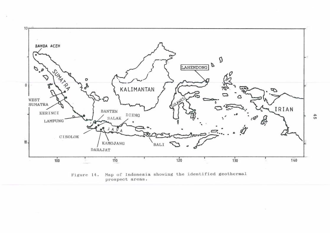
Figure 14. Map of Indonesia showing the identified

geothermal prospect areas .

Figure 15. Map showing original hypocenters calculated by

using single layer velocity model (equation 2),

Lahendong, (PERTAMINA, 1985).

Figure 16. Map showing hypocenters recalculated by using

44

45

46

the first crustal velocity model, Lahendong. 47

Figure 17.

Figure 18.

Map

the

a)

showing hypocenters recalculated by using

second crustal velocity model, Lahendong . 48

Plot velocity (km/s) Vs depth(km) showing

models used in this study (first and second

model), Iceland, and Matsukawa (Japan) .

b) Plot travel-time (8) Vs distance(km) showing

travel-time calculated for

a surface source. 49

Figure 19 . E-W section showing distribution of events at

depth, along latitudes 1 "16.50'-17.50'N, Lahendong

geothermal area.

Figure 20 . N-S sections showing distribution of events at

depths Lahendong geothermal area, Indonesia.

a. Along longitudes 124 " 48 . 5'-49 . 5'E,

50

b. Along longitudes 124 52.5'-53.5'E. 51

Figure 21. The diagram of number of events with depth

showing a peak at shallow levels . 52

6

INTRODUCTION

This report is intended to co.plete the six aonths United

Nations University (UNU) Geotheraal Training Prolraaae held

at the National Energy Authority (N.E.A), Iceland. It contains

two chapters, describina res i stivity aethods applied to explore

,eother.al resources with case histories at Broadlands t New

Zealand, and Hvltbolar, Iceland, and micro-earthquake monitoring

at LahendoDI aeothermal area , Indonesia.

Of the geophysical techniques, electrical methods are .ost

useful and commonly employed in aeotheraal exploration, with

some being used for monitoring too. Bach method has its

advantages and disadvantages , depending on the setting,

purposes and targets of investigations .

In the micro-earthquake monitorina aethod, relocating the

events have been done to observe if there are any discrepancies

between original and relocated events. Studies of hypocenters

distribution in relating to the geotheraal system are presented.

7

PART ONB

1. RBVIBW OF RESISTIVITY HBTBODS

The various resistivity aethods have different capabilities in

probing depth, and in detecting lateral and vertical resistivity

changes. Proble.s arise when combinations of methods yield

different results. Basically the paraaeters that characterize

a geothermal STate., e.g. hiah temperature, alteration alneral

like clays, the presence of electrolyte aqueous solution,

ete, may cause low resistivity anomalies.

The purpose of these methods is to probe the resistivity chanaes

with depth as well 8S map-out lateral contrasts. Chan.ing

current flows through a formation in the earth results in

changing the potential difference at a field rectangular to

the current field. This current field is artificially induced

by injecting the current into the earth. However, natural

current flow can be created occasionally due to (1) the

interaction of solar wind with the earthts magnetic field and

ionosphere below 1 Hz, (2) worldwide thunderstorms above 1 Hz,

and (3) electrochemical, electrokinetic and ther.oelectric

sources within the earth. The probing depths of injected

current is related to the electrode array. Different arrays

are used for geothermal exploration depending on to the

depths of investigations .

1.1. Basic Theory of Resistivity

In this report there is no attempt to discuss in detail the

theory behind resistivity, and only the basic mathe.atical is

presented. The following equation show the potential difference,

V, at a point due to a point source located at distance, r(m),

emanating a current, I(mA), in a homogeneous medium with

resistivity, r{Qm), :

8

For practical work, the current is injected through two current

electrodes which behave as source and sink. Then the potential

difference of V at a point with a distance of r1 from the

source and ra from the sink is :

By measuring the potential difference, V(mV), due to injected

current, I(aA), one can calculate the apparent resistivity:

r •••. = ( V/I)/O ( 1 )

where rapp. and G are apparent resistivity (in gm) and geometric

factor which varies with the electrode arrays, respectively .

1.2. Solving Rising Probleas

1.2.1. Topography

The effect of topography can be solved by avoiding rough terrain

in the field and by 2-D modelling which is done in the office.

1.2.2. Inhoaogeneity

Surface inhomogeneity such as thermal manifestations and the

water-logged grounds of a tropical bush may distort the

observed apparent resistivity. For exaaple. setting the

potential electrodes on inhomogeneous .edia would result too

higher current density in the conductive media rather than in

the resistive one, thus affecting potential drop inversely.

For inho.ogeneities with diaensions much smaller than current

electrodes spacing and located very close to the current

electrodes are considerably less harmful; the electrical

current field may resume its normal pattern away from the •.

One should have at least a qualitative understanding of the

effects of inhomogeneities parallel to the traverse line.

9

In some methods, such as Schlumberger, problem may arise even

if the potential electrodes are set on homogeneous media.

Nevertheless, a Bounding resistivity curve distorted by surface

inhomogeneity may not be resolved during curve interpretati­

on. The problems might be overcome by taking into account

the various potential differences in accordance with the

neighboring current point sources, hence applied a 2-D resis­

tivity computer program.

1.2.3. Practical field operation and portability of

inatruaenta

A compass and tape measure are used to define the traverse

lines. An error of AB spacing due to a bend of traverse line

is very small, about 3% error for an angle of about 10',

Field measurements can be made convenient and less ti.e­

consuming by employing portable instruments especially in

heavy terrain areas. The receiver itself is usually very light.

1.2.4. Data process in.

The observed resistivity data are usually presented a8 a 1-0

model as apparent or true resistivity profiles, apparent and

true resistivity maps at certain AB/2 and depths, respectively.

While a 2-D model is commonly presented as the true resistivity

layering.

Inverting the observed apparent resistivity data into resistivity

layers can be done by either using classical curve matching

or numerical solution aethods. The former is usually used to

get a preliminary interpretation with no sophisticated computer

involved. While the latter is done for detailed interpretat­

ion. It was shown that the apparent resistivities in both

Schlumberger and Wenner arrays at the small and large electrode

spacings tend to be the true resistivity of the first and

last layers, respectively. Projecting a soundin, curve into

layer resistivities may be not so difficult since the curve

is Hummel type.

10

The layer thickness can be d i rectly estimated from the axis

(AB/2,m) by assuming that the dept of the layers is equal to

the sum of the layers with the resistivity values read at the

y-axis. But for the other types of the Bounding curves, e.g.

A, Q and K, the depths of layers are less than the sum of the

layers. Many methods have been modified to get sophisticated

results, and these usually involve the conversion of the

sounding data to Kernel function using Ghosh filter and

determined layering parameters from the Kernel function

using, for example, Koefoed (1979) methods. The I-D inversion

computer program, (N.R.A., Iceland), which is called Ellipse,

was used in this report to inverse the sounding data measured

in 1983 at the Hvitholar geothermal area. This resistivity

program mainly applies a linear filter and automatic iteration

methods. Moreover, the proaram considers the standard deviation

and number of readings of potential differences to determine

the averages of potential values. A problem may arise when

the contrast resistivity between successive layers become too

large, thus giving a sharp slope of the sounding curve.

Whereas the maximum theoretical slope is 45 - . A quantitative

understanding of the correlations of the resistivity layer

with the surrounding zone is desirable.

The 2-D resistivity computer program applying finite eleaent

method, (Sigurdsson, 1986), was also used in this report to

model the B-W resistivity structure at the Hvitholar area.

The program calculates the apparent resistivity of Schlumberger,

Dipole-dipole and Head-on arrays at depths for given arbitrary

grid spacing of layer resistivities model.

11

1.3. Resistivity Array Method

1.3.1. Schluaber,er and Head-On

1.3.1.1. Schluaber.er

Early attempts to measure resistivities in geophysical explo­

ration were based on the two electrode approach rather than on

the four electrode approach. The Schlumberaer method is

described first because it is one of the most common method

used to investigate geothermal prospects nowadays, and has

been applied since 1920, after the works of Wenner in 1915.

The topography effect is stronger at short AB spacing and

shallow depth since the current will flow parallel to the

terrain, rather than at deeper levels and larger spaaings.

Hence, this method has great advantage in investigatina a deep

target rather then shallow formations. Geotheraal reservoirs,

for example, may lie in the ran.e of 500 • to 2500 • depth,

thus requiring only 1000 to 5000 • length of cable since the

probing depth is equal to or less than AB/2. To overcome

topographic effects the 2-D computer program may be used to

calculate the potential at the undulation surface. The

Schlumberger method may give a false picture of the lateral

and vertical resistivity distributions. Within an area

where surface conductivity spreads over several zones and a

thick conductive overburden which absorbs current thus the

layer underneath the conductive layer is unprobed.

The geometric factor can be calculated from the syaaatricsl

electrode array as :

G = z.~ I( l/AK - l/AN + I/BN - I/BM )

where :

AB and MN are current and potential electrodes ar.lengths in

meters, respectively.

12

The apparent resistivity (r •••. ) can then he calculated using

equation (1) by injecting a current throuah current electrodes

AB and then measuring the potential difference at MN.

1.3.1.2. Head-On

This method is an iaprovement of the half Schlumberaer array

and it is very simple interpreting the observed data into

resistivity structures .

However, the method needs a long cable with a length of about

to be equal to or higher than eight times the AB-current

electrode spacing used to create the infinite current source ,

see Figure 2. It was previously applied in China, which has

then been introduced in New Zealand, (Cheng, 1980). It bas

been successfully applied in geothermal areas in Iceland to

detect fracture zones which create a high resistivity contrast,

e.g. the Krafla-Hvitholar geothermal field, (Arnason et al.,

1984).

The geometric factor is simplified to the following relation­

ships due to AC, BC, CM, and eN are infinite :

G = 2*./(1/AH-1/AN),

and

G = 2*./(1/BM-1/BN),

for current electrodes AC and BC, respectively .

1.3.2. Wenner And Dipole-Dipole

1.3.2.1. Wenner

The electrode array consists simply of

and collinear electrodes, see Figure 3.

about the same as that of AM spacing.

four equally spaced

The probing depth is

The method is most

effective in flat or gentle terrain but poses problems in geo­

thermal areas in andesitic volcanic settings where the topography

is rough . One needs a wide flat area to probe deeper resistivity

13

changes that is often absent in such settings, for example, to

probe at depth of about 500 ., a 1500 m (3*&) Ion. wire .ust

be laid out.

Collecting and processing the resistivity data are very

similar to the method of Schluaberger array.

The apparent resistivity, (r. p ,.), can be calculated from the

followin. equation :

r •••. = 2.~.a.( V/I)

1.3.2.2. Dipole-Dipole

Some of the limitations of both the Wenner and Schlumberler

arrays can be overcome by using the Dipole-dipole method.

Al'pin (1950), had all'.ested a modification of the use of the

standard resistivity method which could probe deeper without

using lon.er cables, e.g. Dipole-dipole. The basic advantages

are as follows: a) siaultaneouB measure.ent of vertical and

lateral resistivity variations, b) reduce leakage errors at

both the current and potential cables which is co .. only

present in the practice, c) adaptability to rough terrain, in

as much as cables required are not too long. However, inverting

observed resistivity data into the 1-D layer resistivities is

practically very difficult. The various electrode configurations

is shown in Figure 4.

The Dipole-dipole method is mainly used to detect lateral changes

in resistivity that may be due to faults, fractures, and litho­

logical contacts, rather than vertical changes in resistivity

as in the Schlumberger method.

The coincidence between theoretical curves for Schlumberger and

Equatorial dipole arrays holds only for a medium in which the

resistivity does not vary laterally, (Keller, 1966). Despite

this fact, Koefoed (1979), described the conversion of apparent

resistivity Dipole-dipole into apparent resistivity Schlumberger

method by using the Patella aethod.

14

2. WiNNER AND DIPOLE-DIPOLE METHODS APPLIED AT BROADLANPS GEOTHERMAL FIELD. NEW ZEALAND

The resistivity methods of Wenner and dipole-dipole had been

successfully applied in the Broadlands geothermal fields, New

Zealand. The lateral extent of the Broadlands reservoir was

first determined by the Wenner method with electrodes spacing

of a = 180, 550, and 1100 m, (Risk et al., 1970). The area can

be seen in Figure 5, with the locations of wells, temperatures

at 500 m depth and rate of steam flow. Good geothermal

production zones must have high temperatures as well as high

permeability. However, permeable zones cannot be predicted

from these measurements. For example, a high resistivity

anomaly was mapped out (at north west corner in Figure 5)

where wells later produced high steam flow where as there was

negligible steam flow within low resistivity anomaly. It is

noteworthy that the apparent low resistivity delimited the

extent of the hot water reservoir; however the results can

not be used merely for locating drillholes to find the reservoir.

Besides the Wenner array, Dipole-dipole was also applied in

Broadlands. The method is similar to the maximum array

discussed by Keller (1966), modified a little bit by Risk et

al. (1970). The current source was injected through any two

of three current electrodes (A,B,e) and the potential drop

was measured through a pair of potential electrodes which

were place at rectangular positions . The geothermal field

boundary defined using this method is similar to that of the

Wenner method, see Figure 5.

15

3. SCHLUKBBRGBR AND 8BAD-ON HBTHODS APPLIBD AT HVITHOLAR GBOTHBRMAL ARiA

3.1. Oe010.10&1 Bettinc

The Hvitholar geotheraal area is part of the Krafla geothermal

field , which lies within the south edge of the Krafla caldera ,

in the Neovolcanic zone (north eastern Iceland), characterized

by two active fracture trends i.e . a N-S fissure swarm and B-

W fracture trends. Such structures may indicate the possibility

of a geotbermal reservoir . Until 1979 when steaming ground

was observed, there had been no reported active aeothermal

manifestation in the area .

3.2 . Review of the Geotberaal Area

A shallow larae magaa eha.ber detected by seis.le studies over

the area, most likely causing the high subsurface temperatures .

Geochemical surveys indicated the presence of three major upflow

zones, i . e . Leirhnjukur, Hve r agil and the area south of Mt.

Krafla, (Armansson et al.,1982), however no description are

available yet for the Hvitholar area .

About 23 wells have been dri l led in the low resistivity anomaly,

i.e. wells KJ (1-13, 15), (14, 16-20), and (21-23) at Leirbotnar,

the southern slope of Ht. Krafla and Hvitholar area respectively,

(Sigurdsson et al., 1985).

The higher reservoir pressure in the well KJ-21 compare to the

wells KJ-22 and KJ-23 indicat es a westward flow direction, (Wale,

1985). KJ-23 is, in fact, an unproductive well, even though

the reservoir temperature was hiah enough (about 250 · C)·

About 30 resistivity soundings (Schlumberger) were measured and

also at the same time four l i nes of resistivity Head-on were

measured in the N-S and E-W directions over the Hvitholar geo­

thermal area, (Arnason et al . , 1984).

16

The resistivity substructure had been previously modelled by

calculating apparent resistivity sounding independently from

the apparent resistivity of Head-OD, because the unavailability,

then, of a computer program to calculate the apparent resist­

ivities of different methods simultaneously, see Figure S.

In this study, the calculated apparent resistivities of both

Schlumberger and Head-on methods will be presented.

3.3. Resistivity Modellin.

Bight measured resistivity Bounding data were inverted into

1-D layer resistivity model with the Bllipse program, utilizing

the Vax computer installed at the National Energy Authority,

Iceland. These results were then used to construct a 2-D

resistivity model by simply joinin, resistivity layers.

Afterwards the Head-on apparent resistivities were taken into

consideration. The 2-D resistivity model is modified until

there is good match between the calculated and observed

apparent resistivities both for Sounding and Head-on by the

trial and error method, see Figure 7. The apparent resistivity

soundings calculated at places from the west to the east,

Krl15 , 114, 109, 108, 106, 105, 116, and 122, appear practically

similar to that of the observed ones, especially at deep

levels, as can be seen in Figures 8a and b. The calculated

apparent resistivities of Head-on method gave a good match,

for AB/2 = 250, 500, and 750 ., see Figure 9a, b, and c. The

poor match at the west end of the section for AB/2 = 250 m, is

due to the topographic effects where the measurements had

been carried out in the valley, (Eyjolfs8on, pers. comm.).

To get an impression of the l ocations of wells in relation to

geothermal system in this area, the top conductive (is less

than 20 am) layers and the resistivity variations within the

conductive layers are plotted, see Figure 10 and 11. The top

conductive layers in perspective viewing at angle of tilt and

rotation of 30 · and 225"N, respectively, were plotted (see

Figure 12) although the locations of wells were just approximated

due to the limited capability of the program. It still shows

17

a fault - l i ke structure with a N-S strike at the top conductive

layers but it is not clear at the bottoai the structure may

be hidden .

18

4. DISCUSSION

The Wenner and Dipole-dipole methods were successfully used in

delineating the reservoir boundary in New Zealand, due perhaps

to the relatively flat topography and the lack of abrupt

variations in resistivity. However. the effectiveness of the

Wenner array is not yet fully assessed since the subsurface

resistivity structures have not been modelled yet. and the

apparent resistivity values have not been compared to observed

ones .

It is unlikely that changing the 2-D resistivity model in order

to fit the calculated and observed apparent resistivities at

Krl08 could be resolved by maintaining the Head-on data un­

changed. Discrepancies in the resistivity Bounding curve may

be caused by the presence of a low resistivity zone of altered

rocks underneath Krl14, since the soundings situated far away

were not affected . However, the conductive layers do not affect

the nearby sounding Krl15, s ince it is located at the edge of

the fine arid model where the resistivity structure of the

adjoining area is not taken into account. In the Schlumberger

method, it is assumed that the layer resistivities will be

laterally homogeneous but not vertically . Hence, this method

works very well in observing variations of resistivity changes

with depth. In contrast, the Head-on method delineates lateral

changes in resistivity. Assuming that the Head-on data

represents the subsurface structures without being affected

by lateral changes in resistivity, a 2-D resistivity model

was finally constructed.

The Krafla geothermal field may probably have a source of heat

coming from the bottom since the magma body may lie at levels

of about 3-7 km, (Einarsson, 1978).

And at the Kr l06 and 109, the 2-D resistivity model shows very

conductive (5 gm) veins below the depth of about 300m surrounded

by rather conductive (10-50 aa) zonesi the very conductive (5

am) and semi-conductive (10-50 gm) zones may possibly represent

19

peraeable saturated hot fluids and iaperaeable aaturated war.

fluids zones, respectively. The I-D resistivity .odel shows

the presence of resistive bodies underlay the conductive

zones as it is shown in Fiaure 8a. If it is the case, the

reversed temperature profiles shown by the three wells at

Hvitholar .ay indicate either outflow of tberaal fluids baving

their source in Krafla or some places at Hvitholar . The

latter one is not doubtful, (Eyjolfsson, pers . co ... ). This

interpretation may also be Bupported by the following evidences.

Firstly, the westward outflow of theraal fluids interpreted

from the pressures observation in the wells. Secondly, the

lack of permeability and heat encountered at the south edge

of the Krafla geothermal field. But, the followin. facts do

apparently not support the interpretation, i.e., a) the

observed resistivity (Schluaberger) data are restricted to

probing depths of about 800 m (AB/2 = 1780 m), thus there is

no information below that depth. And, b) the temperature mea­

surements in the KJ-23 start apparently increasin. at depth of

about 1800 m; the well KJ-23 indicates high teaperatures but

poor permeability .

20

5. CONCLUSIONS

The Wenner and Dipole-dipole methods applied in New Zealand works

well on relatively flat terrain where resistivlties do not change

abruptly. The Schlumberger method applied at the Hvitholar geo­

thermal area did not delimit the area of the geothermal system

since the lateral changes in resistivity occurs very rapidly.

The Head- on method can delineate the structures where the satu­

rated hot fluids present producing the high contrast in

resistivities.

To get a good 2 - D resistivity model both the Schlumberger and

Head-on methods should be applied; the Schlumberger methods

give a hetter resolution of vertical variations in resisti­

vities and the Head-on method in lateral directions .

Contouring the conductive layers obtained from the Schluaberger

method may not help much in delineating the geothermal area of

interest .

The general view of the resistivity distributions over the wide

area including Krafla geothermal field is required to determine

the resistivity substructure at Hvitholar a r ea a bit clear.

21

PART TWO

6. RBLOCATING HYPOCBNTBRS OF MICRO-EARTHQUAKBS MONITORED DURING JANUARY-JUNB. 1985. AT THB LAHBNDQNG GBOTHBB"AL ABHA

6.1. INTRODUCTION

This paper evaluates the results of .ioro-earthquakes monitoring

during January to June 1985 at the Lahendong geotheraal field,

North Sulawesi, Indonesia. The hypocenters were originally

calculated usina a constant velocity model and s-p times. In

this study, they were relocated using two coaputer programs,

i.e. HYPOINVERSB (Klein, 1978) and Basic-Hypo, (Hendoza and

Mor,an, 1985). The former one, written in fortran language,

was applied by using two different simulated crustal velocity

models. These aodels were also used for the application of

the latter prograa, written in basic language. However,

since there were only four seismoaeters available at Lahendong,

and the program needs more seismometers to accurately locate

the events, the results are not presented in this report.

The aim is to delineate, if any, the differences between the

original location and the relocation of events, and in addition

to observe the relation between the seis.icity and aeothermal

areas.

The geothermal prospects in Indonesia, are shown in Figure 14.

The geothermal fluids which may be produced from these areas

will be used to supply a power demand of about 300-350 MW.,

which should be on line by 1992, (Akll, 1975, and Finn, 1979).

6.2. RBVIBW OF BARTHQUAKB HQNITORING AT GBOTHBBMAL AREAS

Geothermal systeas are generally located in areas of tectonic

activity, volcanism and seis.icity. Bvidences fro. earthquake

studies indicate that the se i s.icity in geothermal areas is

strongly influenced by the reaional structures. For example:

22

a) the extension of the zone of destructive earthquakes in

south Iceland, (Bjorns8on and Einarsson, 1974), b) focal

mecbanisa solutions of earthquakes monitored in the Geysers

geothermal area, California, reflect the tectonics of the

reaional Coastal Range belt, (Bolt et al., 1968), and siailarly,

c) studies of micro-earthquakes in the Hengill geothermal

area indicate a large percentage of tensile crack events,

believed to be influenced by the regional structures of the

volcanic zones. Micro- earthquake monitoring is a passive

observation of naturally occurring seismic events with saall

magnitude, rather than the measurements of waves generated by

explosions or other artificial means. The method has become

widely used in geothermal exploration. Binarsson (1978),

studied the attenuation of S-waves through a shallow (3-7 km)

body, which he suagested that was a magma chamber at Krafla

geothermal fieldj this anomalous attenuation was not observed

at similar depths (Vp = 6.5 km/s) across the volcanic rift zone

in N-E Iceland. A distribution of hypocenters studied by

Foulger (1984), was interpreted to shows two major heat

sources for the Hengill geotheraal area: the extinct Grensdalur

volcanic centre and the active Hengill volcanic centre.

However, the pattern of local earthquakes at the Fly-Ranch,

Canada, did not conform well to the pattern of existing

faults, (Kumamoto, 1978). The passive seismic method appears

to be most effective in locating heat sources at deep levels,

for example, in areas such as Krafla or Hawaii, were geothermal

systems are associated with magma chamber within 2-3 km depth,

(Binarsson, 1978, and Peck et al., 1968), but less 80 in

mapping near surface features.

6.3. GEOLOGICAL AND GEOPHYSI CAL BACKGROUND

6.3.1. Geolo,ical Settin,

The Lahendong geothermal area is within the volcanic oountry

of Minahasa which lies in the inner arc, extends to the Sangihe

volcanic islands in the north and continues on to the Philippine

archipelago, (Bemmelen, 1949 , and Hamilton, 1979). The Neogene

23

pyroc!astic rocks are overlain by Quaternary volcanics consisting

of andesitic lava , brecoia and welded tuff, (Kartijoso, 1982).

Most of the lav8s are brecciated and some of them hydrotheraally

altered. Within the Lahendons aeothermal area there is a

caldera. At present, the depression inside the caldera is

filled with the acid water fro. which the naae of the Lake

Linau comes; linau means acid.

6.3.2. GeophYsical Bxploration

Schlumberger resistivity Boundina profile conducted at the

Lahendona area, (Marino, 1977), showed a shallow conductive

(2.5-5 Dm) zone underlain by resistive (is higher than 10 Dm)

substratum and located between two resistive zones. This

conductive zone was interpreted that may probably indicate

hot water saturated rocks . Since then, intensive geophysical,

geochemical, and geological surveys have been conducted in

order to find a viable deep geothermal reservoir. The results

of geochemical survey were used to infer that the Lahendong

.eothermal area could probably be a hot water dominated

system . Studies of deep exploration wells indicate the upper

reservoir encountered at levels of about 400 and 800 • contains

acidic water with temperatures of about 260 · C. The bottoa

reservoir below about 1500 m has neutral pH fluids with te.pe­

ratures of about 330 ' C, (Surachaan et al., 1985).

6.4. BQUIPMBNT AND DATA PROCBSSING

6.4.1 . Bguipaent

Four seisaoaeters, type H.B.Q . -800 with vertical aeophones .odel

L-4C, aade by Sprengnether were used to .onitor the micro­

earthquakes at Lahendong aeothermal area. These were also

equipped with a time-cube model TS-400 to synchronize the time

during monitoring every two days (48 hours).

24

6.4.2. Locatin. The Micro-Earthquakes

The hypocenters were originally calculated usin. the relation­

ships in the following formula, (PBRTAMINA, 1985):

(2)

where :

d distance of the event froll the seis.olleter in kll,

V. - velocity of the longitudinal wave in kll/S,

V. - velocity of the shear wave in ka/s,

t. - arrival time of the longitudinal wave in 8,

t. - arrival time of the shear wave in 8.

The distance of the event froll each seismometer (d) can be

calculated since the ratio of (V.*V.) to (Vp-V.) is established.

The ratio of 7.5 ka/s was used to calculate the bypocenters due

to Lahendona's crustal structure similarity to the Dien. &eo­

thermal field, Central Java, where laboratory .easurements of

wave velocities in cores ssmpled from the wells and the surface

are available. For comparison, average regional velocities

in the upper crust are estimated to be 5.39 km/s and 2.93 km/s

respectively for the P- and S- waves, (Hars et al., 1980),

giving a ratio of about 6.42 ka/s.

In this study, the events were relocated using the bypocentre

location program HYPOINVERSE by Klein (1978). The upper part

of the crustal velocity model involving layers with linear

gradient was estimated by coaparison with the crustal velocity

model of Matsukawa geotberaal field in Japan, (Baba et al.,

1970), while the middle and lower part were .erely estimated

by assuming that the velocity at depth of about 5-15 ka and

below 30 km are about 5-6 and 8 . 1 km/s, respectively. Matsukawa

was used due to its lithololical and structural similarities

with Lahendong leothermal area. The model was then varied

somewhat to see how it affected the resulting locations. These

two models are tabulated in Table 1, and plotted in Figure 18

which a190 shows travel times calculated for a surface source.

25

A second location prograa, the Basic-Hypo, written in basic

lan~uale (Hendoza and Horaan, 1985), and recently available

at the UNU Geothermal Training Prograaae in Iceland, was also

used to calculate these events . However, since there were

only four seismometers available at Lahendona as shown in

Table 2, and the Basic Hypo program needs aore seisaoaeters

to accurately locate the events, the results are not included.

While the Hypoinverse does not need as many seismo.eters as

the Basic-Hypo, it still requires that at least four arrival

ti.es be input in the computer. Therefore, only events which

were recorded by all four seismometers were included in this

study. These were about 167 out of 500 events (PERTAMINA,

1985).

6.4.3. Ha.nitude

Magnitudes of all of the events were calculated using the

following formula, (Butler, 1979):

H = 108 A - 108 A. + 108 A,. + 108 (2800/G)

where,

M - Magnitude of the events,

A - Aaplitude of reference earthquake,

G - Gain of the earth displacement at 20 HI,

log A. = 1.6 • log D - 1.55,

log Al. = 0.11 D, and

D - Depth of .icro-earthquake.

6.5. RESULTS

The events are in the aagnitude (analogous to Richter aagnitu­

de) range from 0.4 to 3.5. About 80% of the events occurred

at depths down to 9km.

The relocation of events which were calculated using the first

crustal velocity and the second .odel, are plotted on Figure

16 and 17. respectively. The epicenters calculated from the

26

first model, were displaced dramatically fro. the original

ones, see Fiaure 15 and 16. However, no obvious displacement

of events occur due to the change from the first to the

second model, 8S shown in Figures 16 and 17. All three aaps,

however, indicate that epicenters cluster outside the caldera

rim within the area of 125·50-55' and 1·15-20', and only a

few are located inside the caldera rim. The distribution of

events on the surface does not correlate well with existin.

faults. The focal depths of the events calculated by using

the first and the second model also showed slight displacement

as is observed for epicenters locations, and these are absolutely

displaced from the original ones, see Figures 19 and 20. The

events surrounding the caldera rim are mostly shallow as they

may be observed in detail in E-W and N-S sections crossing

the densest events, see Figure 19 and 20.

6.6. DISCUSSIONS

From the data presented here , the aicro-earthquakes are

significantly concentrated outside the caldera. Only few

events were located within the caldera rim. Two models of the

heat source of the geothermal system at Lahendona could be

postulated to explain the phenomenon

First model :

The hot rocks rest in the region and are cooled from the out­

side by meteoric water. The location of the hot rocks may be

supported by the appearance of thermal manifestations. Hence,

the seismicity is due to the contraction and subsequent

fracturin, induced by cooling hot rocks; meteoric water comes

into contact with hot rocks. Low activity inside the caldera

may mean that the cooling front has not reached this part yet.

Second model :

The hot rocks lay at very deep level inside the caldera. The

heat is carried out vertical l y by meteoric waters forming hot

geothermal fluids.

27

On the way to the surface, the hot fluids flows out towards the

north east, and comes into contact with cool rocks. Hence

fracturing occurs to induce the seismicity. The low activity

inside the caldera is caused by regional strain released

aseismicslly within the caldera because of very hiab teaperature

which may reach at least 400·C within a few ka fro. the

surface. The temperature about 350·C has been encountered in

the wells at depth of about 2ka at Lahendong and at the other

hot water dominated system geotheraal fields, e.g. Lahendong,

Dien. and Saisk (Indonesia).

The diagram of number of events with depth shows increasing

number of events down to 3k. and a decrease in number of

events below. This similar fora of the diagram is also seen

in other seismic areas but the peaks occur at larger depth,

from 5 to 10 km, (Meissner and Strehlau, 1982). The shallow

peak at the Lahendong ma possibly be because of high heat

flow here.

There is no clear evidence indicatina a fault-like structural

plane in the E-W and N-S focal depth sections shown in Figures

19 and 20 . But the rather dense events located near the caldera

shown in Figure 20& may possibly be due to a faulting zone at

depth.

A plot between the magnitudes and number of the events is not

presented in this report, since the number of events was only

about 35 % out of the total events.

6.7. CONCLUSIONS

All of the results are still open to question, since they depend

on crustal velocity models. The first velocity .odel was chosen

for Lahendong geothermal area, due to its structural similarity

to the Matsukawa aeothermal area, Japan.

The locations of events seemed not to be affected by small

changes in the velocity model.

28

Two models of mechanism remain plausible for inducing seis.icity

at Lahendong. Firstly, volumetric contraction due to the contact

between hot rocks and cool fluids, or vise versa, and secondly,

fracturing induced by the regional tectonic activity.

The maximum number of events was found at the depth of 3ka.

If the events are caused by the volumetric contraction due to

the contact between hot rocks and cool meteoric water, then at

this depth it may reflect the fracture zones where the geothermal

reservoir exists, otherwise reflecting high heat flow.

6.8. SUGGBSTION

An seismic explosion survey should be done 88 soon as possible

which may refine the crustal velocity model, presented in the

report, at Lahendong aeothermal area. More seismoaeters

should be used in monitoring micro-earthquakes to ensure the

accuracy of the results and to study focal mechanisms besides.

The additional seismometers in the area of dense events will

better constrain their focal depth.

To remove some of the uncertainty about the model of the geo­

thermal system at Lahendong, it may be worth drilling in the

area of the dense events. If the first model is correct, a

zone of high rate of heat exchange may encountered.

29

ACKNOWLBDGBHBNT8

The author would like to acknowledge National Energy Authority

and PBRTAHINA Mana.ements for permission to publish the data

in this report. My grateful thanks are extended to Dr Brynjolfur

ByjolfsBon and Dr Pall EinarSBon for supervising, reading, cor­

recting the manuscript and making many valuables suggestions

for its improvements.

Special regards to Dr Jon Steinar GudaundsBon, the director

of the United Nations University Geotheraal Training Prograa.e,

for his guidance and valuable advice.

I am also indebted to Hr Slgurjon Asbjornsson, Hr Bessi

AOalsteinsBon, and Hiss Anna Haria Sverrisdottir, staff of

UNU Geotheraal Training Programme, and Miss Olafia, land- lady,

for taking care during attendina the Geothermal Training

Programme in Iceland.

30

REFERENCES

Akil, Is.et, (1975) : Development of Geothermal Resources in

Indonesia. Proceedings of the Second United Nations Symposium

on the Deve l opment and Use of Geothermal Resources, Vol. 1,

11-15.

AI'pin, L. H. , (1950) : The theory of dipole soundin,. English

translation, Geotoptekhizat.

Araansson, GislasoD, H.,G., HaukssoD, T . , V., (1982) Magmatic

gases in well fluids aid the mapping of the flow pattern in a

geothermal system. Geochim., Cosmoehim . Acta , 46.

Arnason, Ko , Byjolffsson , B. , Gunnarsson, K., S •• undsBoD, Kt

BJornsson, A" (1984) Krafla - Hvltholar, Jar6frre6i og jar6e61isfre6ikonnun, 1983. OS-84033/JHDo04, Reykjavik.

Baba, K. , S . Takai, G. "atauo, and K. Katagiri, (1970): On

the reservoir at Matsukawa geothermal field. United Nations

Symposium on the development and utilization of geotheraal

resources. Section VII, reservoir physics and production

management , VII/11, Sept. 28, Pisa .

Beaaelen, R., W. , Van, (1949) : The geology of Indonesia.

Gov. Printing Office, Hartinus Nijhoff, The Hague, Nederland ,

Vol. lA.

Bjornsson , S. and Binarsson, P., (1974) : Seismicityof

Iceland. GeodynamicB of Iceland and the North Atlantic Area

(Edited by Kristjansson, L., D. ) , 225-239. Reidel, Dordrecht,

Holland.

Bolt , B. A. , Loanit, C., and Mc Evilly, T. V. , (1968) :

Seismological evidence on the tectonics of central and northern

California and Mendocino escarpment. Bull. Seim. Soc. Am .

58, 1725-1767.

31

Butler, D., (1979) : Notes on Seismic for aeotheraal energy.

Microgeophysics Corporation, Colorado, V.S.A.

Cheng, Y.W. (1980) : Location of near surface faults in

geothermal prospects by "Combined head-on resistivity profiling

method". Proceeding of the New Zealand Geotberaal Workshop.

Binarsson, P., (1978): S-wave shadows in the Krafla caldera

in NE-Iceland, evidence for a magas chamber in the crust.

Bull. Volcanol . , Vol. 41-3.

Finn, D. F. X" (1979) : Geothermal Developments in the

Republic of Indonesia - 1979 . Geothermal Energy Institute.

Geothermal resources Council , TRANSACTIONS, Vol.S., September.

Foulger, O. R., (1984) : The Hengill Geothermal Area: Seismo­

logical Studies 1978-1984. Science Institute University of

Iceland, Dunhaga 3, 107 Reykjavik.

Ha.ilton, W., (1979) : Tectonics of the Indonesian Region,

Geological Survey Profess. Paper, 1078, pp. 159-189.

Hars K. Gupta, Tzeu-Lie Lin, and Ronald W. Ward, (1980) :

Investigation of Seismic Wave Velocities at the Geysers

Geothermal Field, California . Geothermal Resources Council,

vol. 4.

Kartijoso, S . , (1982) : Borehole .eoloay of well Lh-2 Lahendong

High Temperature area, N- Sul awesi, Indonesia. UNU Geothermal

Trainin. Prograame, Iceland, report 1982-11.

Keller, G., V., and Frischknecht, F., C., (1966) Electrical

methods in geophysical prospectin.. Per.amon Press, New York.

Klein, F., W., (1978) : Hypocenters location program inverse.

V.S.G.S., Open file report, 78-694.

32

Koefoed, 0., (1979) : Geosounding Principles, 1. Elsevier

Scientific Publishing Company, Amster dam, Oxford, New York .

Kuaaaoto, L., (1978) : Microearthquake Burvey in the Gerlach

Fly Ranch area of north-western Nevada. Quterly, Colo. School

of Mining, in press.

Marino, (1977) : Penasunaan cars tahanan jenis dan gays

be rat pads eksplorasi Panssbumi d i daerah kenampakan panssbumi,

Lahendong, Tompaso, Sulawesi Utara. Lang. Bhe Indonesia .

Unp!ub., Geol. Survey Indonesia Report.

Meissner, R., and Strehlau, J., (1982) : Limits of stresses

in continental crusts and their relation to depth-frequency

distribution of shallow earthquakes, Tectonics, vol. 1, 73 -

89 . American Geophysical Union.

Mendoza, J., and Mor.an, D., (1985) Basic-Hypo. A Basic

language Hypocenter location program user's guide . School of

earth sciences. Stanford University publications, Stanford,

Geological Sciences, Vol. XIX, number 1.

Peck, D. , L., and Minaka.i, T., (1968): The formation of

columnar joints in the upper part of Kilaulan lava lakes,

Hawaii, Geol. Soc. Amer. Bull., 79, 1151 - 1166.

PBRTAMINA, (1985) : Pengamatan gemps mikro di daerah Lahendong,

Sulawesi Utara. (" Micro - earthquakes monitoring at the

Lahendong area, North Sulawesi"). Internal report. Unpubl.

Risk, O. F., Macdonald, W.J.P., and DawBon, G.B., (1970) : D.e. Resistivity Survey of the Broadlands Geothermal Region, New

Zealand. Geothermics (1970) - Special Issue; U.N. Symposium

on the Development and Utilization of Geothermal Resources, Pisa,

Vol . 2, Part I.

33

Sigurdsson, 0., SteinariasBon, So , S., and StefanS8on, V.,

(1985) PreSBure build up monitoring of the Krafla geothermal

field, Iceland. Tenth workshop on Geothermal Reservoir

Enaineering, Stanford University, Jan., 22-24.

SigurdssOD, Ro, (1986) : Lecture at the Geophysical sectioD,

National Energy Authority, Iceland.

Surachaan , S ., Tandirerung, S., A" and Robert, D. , (1986) : Preliminary results and future promises for the development

of the Lahendong geothermal field, North Sulawesi, Indonesia.

Pertamina internal report, f or publ . , in prep.

Wale, A" 1985 : Reservoir engineering study of the Krafla­

Hvitholar geothermal area, Iceland. UNU Geothermal Training

Programme , Iceland. Report 1985-10 .

34

Model Velocity , km/s Depth, km

First 2.50 0 5.00 2.50 6.00 15.00 8.10 30 . 00

Second 3 . 00 0 5.50 9.00 6.00 15.00 8.10 30.00

Table 1. Atteapted crustal velocity .odel. used to calculate the bypocenters of .ioro-earthquakes aonitored during January - June, 1985, Lahendong, Indonesia.

Station No . Longitude Latitude Blev. E N (a.B,l., .)

41 124' 46' 40' J 1 • 16' 15 J J 600 42 124' 49' 53 I , 1 • 14' 28" 700 43 124' 52' 22 J • 1 • 15' 08" 800 44 124' 50' 52 J , 1 • 19 ' 20" 700

Table 2. Shows coordinates of the seisaoaeter locations.

35

A M N B 1'-----1-. -1-----1

Figure 1. The electrode array of Sclumberger.

A M N B 1----=----1 ---...:Q~--I ----.:Q"---

Figure 3. The electrode array of Wenner.

1 C

I~ QC ~8 AB

A M Q N B 1 1 __ 1 1

Figure 2. The electrode array of Head-on.

'>-. / -, @

, @ , @

, @ , , , , , , , , , , , , , , , , , , , , , , , , , , , , , , , , , , , , ,

~' ~ ' ,..L.\ ' ,...k\ e

J , , ,

Figure 4. The electrode array of dipole - dipole, a) azimuthal, b) radial, c) parallel, and d) perpendicular.

o.

b.

F i gure o.

•• _.

• ! ,

o.

t

!

36

y ::.:: , ~.~ "" ........ ",._w._ " ,_ ...... , \ f"1 '_' ''C, " ........... '> .. __ .....

, , ,

" J. " , " ,

.... ,

.. , .... , .....

M .

..

..

.. . ." .. " ," •

..

•

t ) .. .. , • •

..' ....... N

..

..

•

.. n •

..._--,-__ I,.

, •

Geothermal fiel d bo undary J Broadlands, New Zealand. a ) by applying We n ne r method with a =550m, and b) dipolp - dipole method.

.~

'"

, .. ...

'00

.. • I'OO , ., " • ' 00

" •

v .-'" 50

6

200

•

V

Figure 6.

IM-I I$ I I

. ., ... ""'" '000 -- .~

1100 ,"00 ,-' 00 600 ~ ." ! " '0

200 -•

15

'00 MOO_

r ---- - -.~·IU '~' '' I .~.~

'"A '0 '00

'0

15 "

'00

200 60

37

• ... ... .oo " . '" '" '0 '0 '0

-5

!

a.

KRAFLA-HVtTHOLAR V5 - 3

Tvivio TlJLKUN, VIONAMSSNID

oo • , O. ... ... - ~ ... ,000

" 80 50 1

'" 60 100

I 60

' 0 '0 20

VS·, t- - - - ---, .... 00. . w-t09 KR_~

"-t -6

120

50

60 60

5 l '0 ,

100 60 '0

_ 00

b. KRAFLA- HviTHOLAR SL · '

SNID TVIV ID TULKUN , VICNAMS

.~.". n·", -• --» • ". 100 75

'00

20 -

" 2 ,

,

20 5

•

2 - D resistivity model of Hvithol a r geothermal area, E-W section, constructed fro m a) Head-on and b) Schlumberger methods, (Knutur Arnason et al., 1983).

w 38

Kr 122 Kr 116 Krl05 Krl0G Krl09 Krl0B K r 114 K rl15 , , I , - L

100 - 500 25 25- 50

12 5 •. I 5 -100 - 500

10- 50

10 - 50 100 - 200 2-5 10-25

10 50

500 •.

r-

5 5

5 100

2-5 10 - 50 2-5

100 - 500 1I lOO 1 1 5 1

Figure 7. 2 - D r e si s tivity model of E- W sect10n, Hvitholar geothermal area, constructed from the combination the Schlurnberger and Head- on method.

11:, 122

The location of soundings are in Figure 10 and 11.

lOOm

He a d -on res istivit7 profiling . o o 500

Scull! loo0m

E

r-

w

500

E

1500

3 9

Kr 122 Kr116 Kr105 Kr106 Kr109 Kr 10B K r114

Figure 8a. Contour of ob s erve d appar ent resistivities (Schlumberger), E- W section, Hvitho!ar, Iceland.

Kr 122 - Resistivity sounding s tation.

~15~ - Re sistiv i ty contour line in Qm.

E K r 11 5

w

40

Kr 122 Kr116 Kr105 Kr106 Kr109 Kr10B Kr 114

Figure 8b. Contour of apparent resistlvities (Schlumberger) calculated by using 2 - D resistivity model of E-W sect ion, Hvitholar, Iceland.

Kr 122 - Resistiv i ty sounding station.

15 / - Res ist ivity contour line in Slm. /'

E

K r115

w E RHOc A C - AB)

Q . RHO( AC - 1\8)

... - -.,.- ...... -...... ., t'!lOO

/ / ObO!c r vcd

\ '"' \ RH O (ABlh 250m) '" ."

r-'-"--'--'- · 1 · ·· ~ - " - .... ..... ··· . ···..-... ·· r-,·· l .~-,---r-.. -"T""". '- ' r-'~~~' , -1500 - 1000 - 500 0 !lOO 1000 1!100

Dist.ance, Ill.

b. RHO( AC -AB)

RHO( 4C - AB)

/ Calcul ated

Distance , m.

RHO( AC - AB)

RHOcI\C _AB)

c. . S ! ---- , 'X -' -' 7-- 1$00

Obser ved Calculated

DiBtance, Ill.

'"

."

,

-100

- 2110

."

,

- 100

."

,

-100

, ~ ,

, , • ~ o

, , ~ o

Figure 9. Appare nt resistivities of Head - on method, obse rved and calculated by using 2- D resistivity model, E-W section, Hvitholar, Ice land .

a) For AB/2 =250m, b) SOOm, and c) 750m.

41

42

Figure 10. Map showing top conductive (~ 20 2m) layers at the Hyitho!ar geothermal area, Iceland.

Geothermal exploration ~ell.

Resistivity sounding (Schlumberger) Krl08, used to canstuct 2- D resistivity model.

43

Figur~ 11. Map showing the resistivity variations (Qm) within the conductive layers, Hvitholar, Iceland.

Geothermal exploration well.

Resistivity sounding (Schlumberger) Krl08, used to construct 2- D resistivity model.

44

N

Figure 12. Shows top conductive layers in perspective viewina at anales of tilt and rotat i on of 30 . and 225 - , respectively, Hvitholar, Iceland. The locations of wells are approximated.

101r-----------------------------------------------------------------------r

o

10

SANDA ACEH

WEST SUMATRA

KERINCI

LAMPU NG

o

J>

~-D BANTEN

) '-.J'-...,j KALIMANTAN

,~ALAK DrENG •

elltJAVA '---=:.. D.

,-0

Q

LAHENDONG' ~ "

~CQ'

'.

\)

t:;:!, ~ t:t:. •

ZJ~ a a '""""

IRIAN , . O'~" ~"

•• '. ' ':r# ~ . = . IJ' .

• CISOLOK I KAMO J ANG DARAJAT

~~.C ~?E?~'"

100

BALl ~ • .f/

110 110 130

Figure 14. Map of Indonesia s h owi ng the identified geothermal prospec t area s.

140

... '"

-l 0

.' ,.

" r • •

124"4 5 '

0 0 0 0

0 0

0

0 0 0 00 0 • 0

4 0

• 0 • • • 0

0

0 8 0 0 00 0 0 0 0 0 0 •

0 0 0 • 0 0 °oooCfJ 0 o 00

• • o· 0 0 3. • • • 9 0

0 00 • • • •• 0 0 •

0 0 0 0 • • 0.' • 0 • 0 • • 00 0 0 0 ~ ~ .0 o. • o· 0 0

0 • 0 0

2~ • 0 0 0 0 0 0 0 0

0 0 0 0 0 00 0 00° ··op o 0 •

" • 0 • . 0·· .. 0 0 ° cl} ... • • • f . • °0 0 0 • /,

• 0 '. 0 0 000 L.hendong. ~ • o 00 0

1~:0 '0

0 0

.' 0 0 0 0 • 0 0 ~ • 0 0 • 0 § 10 - - - • • • 0

b - • .0 Le g e nd •

• Lk.Linau 0 • 0 Location of sei~ometer . nu~be r I • 0 O· • • • • • 0 0 • \<t e ll nu mber Mt. Tampusu "/,,3 0 0

I 0

Events wi t h ma,ni tudes • 04 • • 0 •• Ev e nts with ~agnitudes • 0 o • 0 0 • .. ( oLcllra ri. • • 0 0 Thermal manifestatuions 0

Hot apri n. 0.2 0

00

Fu.a roles • • 0 • •

• 0

50

Figure 1 5. Map showing origin a l h ypocenters c a lculated by

using single layer veloc i ty model (equation 2),

Lahendong, (PBRTAMINA , 1985).

1-1"20 '

0

0

0 0

0

0 0

0 0

0 0

0 0 •

• .po

'" 0

00

0 1-1"15'

0 0 • 0

0

124° 55 '

ft· '5' sa' 'j'j ' '25'" I r I I I ~

,~

~,~

ntOI 25 I 8$ TO gllS

NO I1f ~llIII.RIS ". II'IX"" ,.' IIIX MS t.2S 5CC IIIX OIH 2.1.QI IIIX 00 se.' .QI

Da'llI 1011

U 1 13 '

I .• · sa .• IfI&NITUlE

I •• • 5.81

Figure 16, Map showing hypocenters recalculated by using

the first crustal velocity model, Lahendong,

'.H , .. e .. · ..

~ (Illderll rim , fQult

'. "'11l no.l

. ' S.i s . o."hr

". ... ..,

o

Figure 17.

o .' o

o

o o

Nap showing hypocenters recalculat e d by using

t h e second crustal velocity model, Lahendong.

• ""-'

.~

"',., ~_2$I" TO ;'15 .. " """"""'" H. - g:p ,.' I!AX RIC5 '.25 5EC _(1111 2.' 101 _ E:IIl SI •• 101

DU'" nOli ' .l1li. SI." ... , .... •.• - 5 ••

••• ••• e '·· '\: ~ (Qldero rim

_'" Fo.vll 1. W,II no. 1

.' S,i'.olut,r,1 ... .,

10

e x 20 ~ -~ w

0

30

8

49

Q Velocity , km / so o 4 6

r---~_~ 2

Sec ond model_

First mOdel /

f(eland -_

b

0 0

0 • 0

Sec ond model 0

8

--

•

6 _ "" 0

0

~ 0

w 0 e Fir s t model -4 - 0

w 0 > d

i " ... 2 • 0

• e

10 20 30 4 0 Dis t ance , km.

Figure 18. a) Plot velocity (km/s) Vs depth(km) ShOldng

models used in this study (first and second

model), Iceland, and Matsukawa (Japan).

b) Plot travel - time (9) Vs distance(km) showing

travel - time calculated for a surface source.

50

I caidera 0.00

W E

t:P A .t. ... ~ . ...

- 5.00 .t. Iti. ... ... ... ... 6

... E x-IO.OO ~

.t. ~

~

~

0 .t. - 15.00

0 Skm I

-20.00 40 . 00 45 . 00 50 . 00 55.00

Figure 19 . E-W s ection showing distribution of events at depths) along latitudesl ' 16.5' - 17.5' J Lahendong geothermal area, Indonesia .

Legends :

Events calculated from the first crustal velocity model.

Events calculated from the second crustal velocity model .

60 . 0

51 0.00

S .0. . N

• !'.o. • a .

.0. • ,. lA • .0. ~ t.

-5.00 .0. ~

.0. • • .0. .0.

E x

~

~-10.00 ~

~

"

E x

~

-15 . 00

-20.00 10 .00

0.00

-5.00

0L. ____ -"'5 k m

S

• ...

Legend

15.00

... ... .0. ~

... .0.

•

Events calculated from the first crus tal velocity model.

Events calculated from the second crus tal velocity model.

20.00 25.

.0. .0..0. b. N .0.

...

.0.

~ -10.00 • ~

"

-15.00 Legend

0.~ ___ ......::..5km

.0.

Events calculated from the first crustal velocity mode l .

Events calculated from the second crustal velocity model.

-20.00 +---------------.---------------,---------------~ 10.00 15.00 20. 00

F igure 20. N- S sections showing distribution of events at dept hs, Lahendong geother.al area, Indonesia. a. Along longitudes 124 ' 48.5~- 49.5 ' E, b. Al ong l o ngitudes 124 ' 52.5 ' - 53.5 ' E.

25 .

E .x

:r:

~-s

6-7

I-- 10-11 CL

w o

12-13

1~-1 5

D

0 0

16-17 ·

18-19 ·

~

0 0

52

NUMBER OF EVENT - - N N W D !" D ~ D

c. 0 c. 0 0 0 0 0 0 0

Figure 21. The diagram of number of events with depth

showing a peak at shallow levels.