applicationsofmathematics - dml-cz · applicationsofmathematics milanpokorný...
TRANSCRIPT

Applications of Mathematics
Milan PokornýCauchy problem for the non-newtonian viscous incompressible fluid
Applications of Mathematics, Vol. 41 (1996), No. 3, 169--201
Persistent URL: http://dml.cz/dmlcz/134320
Terms of use:© Institute of Mathematics AS CR, 1996
Institute of Mathematics of the Academy of Sciences of the Czech Republic provides access todigitized documents strictly for personal use. Each copy of any part of this document must containthese Terms of use.
This paper has been digitized, optimized for electronic delivery and stampedwith digital signature within the project DML-CZ: The Czech Digital MathematicsLibrary http://project.dml.cz

41 (1996) APPLICATIONS OF MATHEMATICS No. 3, 169-201
CAUCHY PROBLEM FOR THE NON-NEWTONIAN
VISCOUS INCOMPRESSIBLE FLUID
MILAN POKORNY, Olomouc
(Received October 25, 1994)
Summary. We study the Cauchy problem for the non-Newtonian incompressible fluid with the viscous part of the stress tensor r (e) = r(e) — 2uiAe, where the nonlinear function r(e) satisfies rz-j(e)ez-j ^ c|e|p or Tij(e)eij ^ c(|e| + |e |p) . First, the model for the bipolar fluid is studied and existence, uniqueness and regularity of the weak solution is proved for p > 1 for both models. Then, under vanishing higher viscosity txi, the Cauchy problem for the monopolar fluid is considered. For the first model the existence of the weak solution is proved for p > ^dr r, its uniqueness and regularity for p ^ 1 + ---rj • In the case of the second model the existence of the weak solution is proved for p > 1.
Keywords: non-Newtonian incompressible fluids, Navier-Stokes equations, Cauchy problem
AMS classification: 35Q30, 76A05
1. INTRODUCTION
a. Equations and constitutive laws.
Let n = 2 or 3. The motion of incompressible viscous fluid in Rn is described by
the system of equations
(1.1) d i v u = ^ = 0 , OXi
(1.2) , _ + ^ _ = _ _ + , , . . , = i > 2 , . . . , „ .
Here the equations (1.1)—(1.2) express the balance of mass and the balance of mo
mentum, respectively. In the equations u = (1x1,1x2, •• • ,wn) represents the velocity
field, g = const > 0 the density, f = (/1, / 2 , . . . , fn) the specific body force and r^-
are the components of the stress tensor. All quantities are evaluated at (x, t), where
169

x = (a;i, .r2 , . . . ,xn) is the actual position and t the present time. When no misunderstanding can occur, we will write only u instead of the correct u(x, t). Hereafter, for simplicity in writing, we put g = 1 and use summation* convention.
In order to make the system of equations complete it is necessary to prescribe the constitutive relation for the stress tensor. Due to physical considerations, the stress tensor is decomposed as
(1.3) Tij = -irSij + rV,
where TT is the pressure, Sij is the Kronecker delta and TV is the viscous part of the
stress, which must be defined by a set of constitutive relations.
In the present work we will assume the stress tensor TV of the form
(1.4) TV =T{e)
with r a symmetric tensor, where the components of the deformation velocity tensor e are given by
1 (dui t duj (L5) e- = e-(u) = U ^ + In our considerations the polynomial growth
(1.6) M e ) | ^ Cl(|e| + l e r 1 ) , Cl > 0,p > 2, |rii(e)Kc1|er1, Kp<2
as well as the strong coercivity condition
(1.7) Tij{e)eij ^ c2 |e|p, 1 < p < oo, c2 > 0
will play an important role. Here |e| means the Euclidean norm of the tensor e, i.e.
(1.8) |e| = (eijeij)^.
We will assume the existence of the scalar potential $ for the stress tensor
^ <^(e) (1-9) ^ W = - f l ^
with t?(-) twice continuously differentiate in IR"2, tf 0, tf(o) = 0 such that we have
for all £ e R£ m :
(1.10) | " - 5 - ~ - f e 6 * > C 3 ( l + | e r 2 ) ^ £ ; « , P ^ 2 , deijdeki
•f^T-tiifa > C3|e|"-2$y£;.i. P < 2-deijdeki
170

It is possible to show that (1.7) is a direct consequence of (1.9), (1.10) and the fact that ů(o) = 0.
There are several phenomena which appear studying non-Newtonian fluids: shear thinning and shear thickenning, ability of a creep, ability to relax stresses, presence of normal stress differences in simple shear flow, presence of yield stress. For more detailed description see [17]. Our model includes shear thinning (p < 2) and shear thickenning (p > 2).
1.11. R e m a r k . Generally it is possible to assume that тv is a function of Du.
However the principle of material frame indifference (see [9]) implies that тv can
depend only on the symmetric part of the velocity gradient.
We have in mind two exampies: first, for p > 2
(1.12) тi:j(e) = (џ0 + џi\e\p'2)eij
with /x0, џi positive constants and second, for p Є (1,2)
(1.13) îïi(e) = | e | p - 2 c ť i .
It is an easy matter to check that the potentials
1 ľeí;e«; u-2 #(e) = õ / (Џo+ Џis 2 ) d s
for p > 2 and 1 ГЄiІЄ £-2
i?(e) = - / s - ds 2 Jo
for p < 2 satisfy the assumptions (1.9)-(1.10).
We will also study separately the model (1.12) for p < 2 for which we will be able
to prove the existence of a weak solution for all p > 1. Of course, we have to modify
the conditions (1.6), (1.7) and (1.10). The condition (1.6) will be the same for both
p < 2 and p ^ 2, instead of (1.7) we have to use TІJ(Є)ЄІJ ^ c( |e | p + | e | 2 ) . The
condition (1.10) must be replaced by Q^.$klţijţik > c 3 (l + \e\p~2)ţijţij. We will call this model the perturbated linear model.
b. Problem formulation and survey of results.
1.14. Definition. Let u 0 : IRn н-> (Rn, f: Qт ь-> (Rn be given functions. The
problem (CMN) denotes the following: to find u(x, í) , 7г(x,t) solving (1.1), (1.2),
(l.З)-(l.ľ), where u(x, 0) = u 0 (x) . The letters (CMN) abreviate the Cauchy problem for the Monopolar Non-Newtonian incompressible fluid.
171

In Chapter 3 we will assume the viscous part of the stress tensor in the form
(1.15) TV = r ( e ) - 2 i u 1 A e , Lti > 0,
where r is supposed to satisfy all the assumptions (1.6)—(1.10). Such fluids are
called bipolar viscous fluids. The theory of bipolar fluids is compatible with the
basic principles of thermodynamics, including the Clausius-Duhem inequality and
the material frame indifference. The thermodynamical principles also imply that the
other higher (third order) stress tensor T{jk must be considered. See [15], [3] for a
detailed description of multipolar fluids. Here we suppose
den (1-16) rijk = 2/f ^гj
dxk
1.17. Definition. Let u 0 : (Rn •-> [Rn, f: QT >-> Un be given functions. The
problem (CBN) denotes the following: to find u(x, t), 7r(x, t) solving (1.1), (V2),
(1.3), (1.5)-(1.7), (1.15), where u(x,0) = u 0 (x). The letters (CBN) abreviate
Cauchy problem for the Bipolar Non-Newtonian incompressible fluid.
In Chapter 3 we will prove the existence, uniqueness and regularity of a weak
solution of the problem (CBN). In Chapter 4 we will study the limiting process
\x\ —> 0 + in order to prove the existence of a weak solution of the problem (CMN). We
will get the existence for p > ^ ^ and its regularity and uniqueness for p ^ 1 + - ^ .
The mathematical theory of the problem for the monopolar fluid was introduced
for the first time by O.A.Ladyzhenskaya (for bounded domains). She proved the
existence of a weak solution for p ^ -g-(n = 3) and its uniqueness for p ^ | ( n = 3).
For details see [8]. The same results were been proved in [10] for the p-laplacian,
i.e. the existence for p ^ 1 + ^ ^ and uniqueness for p ^ n ^ , n - 4. The limiting
passage from the bipolar fluids to the monopolar ones was done for the first time in
[14] and [11].
This paper follows up with the papers [2] and [12]. The former uses a similar
method as the present work, i.e. the authors first solved the problem for the bipolar
fluid and letting fii -> 0 + they obtained a solution for the monopolar case (both
Young measure-valued and weak). In the latter the results were obtained directly
using the Galerkin method. In both papers the following results were proved: the
existence of a Young measure-valued solution for the Dirichlet problem for p > - ^ ,
the existence of a weak solution for the space periodic problem for p > - ^ , its
regularity and uniqueness for p ^ 1 + - ^ . The aim of this paper is to show that
the same holds also for the Cauchy problem, i.e. O = Un is unbounded.
As far as it is known to the authors, there are up to now no results in the case of
a general unbounded domain.
172

2. FUNCTION SPACES, INEQUALITIES
Let n - 2 or 3. Denote I = (0,T) with T > 0, QT = Un x I. The standard notation is used for both scalar (u: Un i-> U or <2r •"->• K) and vector-valued functions (u: lRn »-> Un or Q T J-> Q3n).
We denote by C(lRn) and Cfc([Rn) (k G N or k = oo) £lie space of real continuous
functions on (Rn and ihe space of k-times continuously differentiate functions on (Rn, respectively. The space of real C°° functions on Un with a compact support in IRn is denoted by $(Un) and its dual by $'(Un). Under D^k)u we understand the vector which consists of all possible derivatives of the fc-th order with respect to the space variables, Du = D^l)u.
The Lebesgue spaces of scalar and vector-valued functions are denoted by Lq(Un)
and Lq(Un)n, respectively (q G [l,oo]). The spaces are equipped with the standard norm denoted by || • ||q. The Sobolev spaces JVm'p([Rn) and pVm'p((Rn)n are the sets of all measurable functions, for which the functions and all their generalized derivatives up to the order m belong to Lp(Un) and Lp(IRn)n, respectively. The spaces are equipped with the standard norms and seminorms denoted by || • ||m>9 and I • Im.g. For more detailed descriptions see e.g. [1].
Let s be a noninteger positive number, s = [s] + {s}, where [s] is the integer and {s} the fractional part of s. Let 1 - p < oo. Then the Slobodeckij spaces TVs'p(IRn) (VVs'p((Rn)n) are subsets of the Sobolev spaces W^p(Un) (IVM'p(IRn)n), where
/n,x i. n . . . . v ^ ( f \Dau(x) - Dau(y)\p J , \p
(2A) H . I P = NI W I P + £ / ,x v\nHs}; dxdy <°°-
| a | = w VR»xR» | x - y | t ; p j We will use the following imbeddings and interpolations which hold between Slo
bodeckij and Sobolev spaces:
2.2. Lemma (imbeddings). Let 1 < p < q < oo. Let 0 ^ s2 < si < oo be integer or non-integer. Then VVSl'p((Rn) «-> WS2>q(Un) if
(2.3) i = I - £ L Z * . q p n
P r o o f . See [19, p. 129]. D
2.4. Lemma (interpolation in 5). Let u G fV5l 'p((Rn)n, 0 < s2 ^ s ^ si < 00, 5 non-integer. Then there exists a constant c > 0 such that
(2-5) Hull.,, < c||u||« ,- | |u | | i -»,
where
173

(2.6) s = as1+(l-a)s2, Q 6 ( 0 , 1 ) .
P r o o f . See [20, pp. 181-186]. •
Korn inequality will be used for estimates of the nonlinear term:
2.7. Lemma (generalized Korn inequality). Let <D G W^q(Rn)n D Wli2(Ufl)n,
q>\. Then
(2.8) (J^|e(v?)|dxj ^/f,Mif„
where Kq > 0, 2e{j ((D) = § * + |*f.
P r o o f . See [16, pp. 47-48]. D
The following classical lemma will be used for the limiting passages in the nonlinear term:
2.9. Lemma. Let QT C (Rn+1 be bounded. Let fN: QT »-> R be integrable for every N and let
(i) lim //v(y) exist and be finite for a.e. y € <5T A!-»oo
(ii) ye > 0 36 > 0 such that
sup / | / * (y ) | dy < e VH c QT; \H\ < 5. Iv JH
Then
(2.10) Jim / fN(y)dy= [ lim /jv(y)dy. N->00JQT JQT K->OO
P r o o f . See [5]. D
174

3. W E A K SOLUTION FOR THE BIPOLAR FLUID
In this part we will deal with the problem (CBN). Our goal is to prove existence,
uniqueness and regularity of the system
(3.1) OXІ
(3.2) дщ дщ дt J дxj
= ӘҠ 1 дTij 2ßL д
дxi дxj дxj
(3.3) Uť(x,0) = U O І ( X ) ,
where the nonlinear tensor function r ( ) fulfils the conditions (1.6)-(1.10).
We denote
(3.4) H = {<p e L 2 (IR n ) n ; div <p = 0} ,
(3.5) Vp = {<p £ ®'(Un)n; D<p € Lp(Un)n2; div<^ = o} .
The latter is equipped with the usual seminorm of the Sobolev space W1,p(R.n)n, i e - I • W„ = I • |i,p- Hereafter, u e LP(I; Vp) means that Du e Lp(I;Lp(Un)n2) and
|uU,-(/;v„) = llou||Ll.(/;L>'(R")"2)- W e d e n o t e
(3.6) U = W2'2(Un)nnVp.
We will assume the following about the data of our problem:
(3.7) u0ew2'2(Un)nnH, feL2(I;L2(Un)n).
дu дt
3.8. Definition. The function u £ Lp{I;Vp)nC(I; H)<~) L2(I;W2<2(®n)n) with
S L2(I; L2(IRn)n) is called a weak solution of the problem (CBN) if
(3-9) / ~ o 7 ^ d x + / uj^-L(pidx+ / Tij(e(u))eii((/?)dx JR" Ol JRn OXj JRn
f de{j(u) deij((p) f + 2/xi / JK JK d x = / /*<Ddx
JRn OXk OXk JRn
is satisfied a.e. in I for every ip € U.
In order to be able to use the Galerkin method, we need to find a countable dense
subset of the space U with special properties. In fact, we need the functions of this
175

subset to be smooth, have compact support and zero divergence in [Rn. The existence of such a subset is ensured by the following lemma.
We denote
%(Un)n = {<pe$(Un)n; div<D = 0} .
3.10. Lemma. There exists a countable subset of the space @o(Un)n which is
dense in U.
P r o o f . As ^ ( R n ) n is dense in W2'2(Un)n and Vp, we have that 2)(Un)n is dense in U. The separability of $)(Un)n yields the existence of a countable subset of Q)(Un)n which is dense in U. We denote its elements {<^n}^Li- These functions have generally a non-zero divergence.
We denote gn = div(/?n, where evidently gn G &(Un). Let us solve the problem
(3.11) divipn=gn.
In [4] it is shown that there exists a solution ipn G $(Un) such that
( 3 A 2 ) | | ^ n | | 2 , 2 ^ C i | | a n | | i , 2 ,
(3.13) ||V>n||l,p^C2||On||p.
We denote
(3.14) w n = (Dn-</>n.
Now, let v be an arbitrary element of U and e a positive number. Then there
exists <pn G ^ ( R n ) n such that
(3.15) \\ipn - V||f7 = \\ifn ~ V||2f2 + \<Pn " v | l , p ^ ,
1 + Ci + c 2
see (3.12), (3.13). Then (divv = 0) | |wn - V||t/ = ||(Dn- V ~lpn\\u
^ \\Vn - V\\U + Un\\u
^ +ci||div((/?n - v)| | i | 2 +c2||div((Dn - v) | |p ^ e
1 + Ci + c2
and the set {wn}n^=1 is dense in U. •
176

The next two simple lemmas will be used for the apriori estimates. Their proofs
are direct consequences of the fact that /R n |2(f )|2|£|2A: d£ is an equivalent seminorm
on VVfc'2(lRn), which can be found e.g. in [16]. Here C(£) is the Fourier transform
of u.
3.16. Lemma. Let u G L2(Rn), D^u G L2{Un)n2. Then Du G L2(Rn)n and
(3.17) \\Du\\2^c3\\u\\2\\D^u\\2.
3.18. Lemma. Let u G JV2 '2(Rn), n ^ 3. Then u G L°°(Rn), i.e. there exists
C4 > 0 such that
(3.19) esssup|ti(x)| < C4||u||2,2-xGR n
Now let { w n } ^ = 1 be our countable dense subset from Lemma 3.10 (after eliminating zero and linearly depending functions).
N
3.20. Definition. We say that uN(x,t) = £ cf (tjw^x) is the Galerkin ap-i = i
proximation of the solution of the problem (CBN) if
P21) / i S ^ ^ w W w d x •l«" v.t? + / r i j (e (u w (x , i ) ) )e i j (w a (x) )dx
+ 2^ J 3e i j (u j V (x ,<) )9e i J (w"(x) ) d x
jR« dxk dxk
- / / < ( x , * X ( x ) = 0 Vwa a = l ,2 , . . . , iV. JR"
Using the Caratheodory theorem (see [7]) we get the existence of the Galerkin approximation locally in time. From the apriori estimates in L°°(I; H) we have the existence on each time interval (0,T), T < co.
3.22. R e m a r k . For the Caratheodory theorem we need that the matrix with the elements a / a = JRn wl
{wf dx be regular. It is the so-called Gram matrix, and it is known that the Gram matrix is regular provided { w a } ^ = 1 are linearly independent.
177

3.23. Lemma. Let u0 G H, f G L2(7; L2((Rn)n). Then the sequence of Galerkin approximations satisfies the following uniform estimates:
(3.24)
(3.25)
(3.26)
, -V|i llu I|L°°(/;L2(R")TI) ^ c5,
ll^uN|lL^(/;L^(Rn)n2) ^C6>
l|uiV||L2(/;W2'2(R-)") ^ c7-
Proof . Multiplying (3.21) by cN(t) and summing up the equations we get (using the fact that fRn uN ~^-uN dx -= 0 for divergence free functions)
_dl dí2
/ I U ^ p d x + Z TiMvL^ЂЄij^dx JR" JRП
+ 2џ. L ae i j (u A f )ae i j (u w )
дxk дxк
dx = / / i t u^dx.
Integrating over (0, t) and using the coercivity condition (1.7) and the Korn inequality (2.7) we obtain
(3.27) i | |u"(*) | |2dí + cp / V u ^ d ť + Č ^ f\\D™VLN\\ Jo Jo
I í í f i u ? 1 JO JRn
dxdí| + i | |uo| | l .
Taking the first term on the left hand side we get
(3.28) | |u w (t) | | l ^ / ' ||f | | a(l + Hu^llI) dt + HuollI, JO
which after employing the Gronwall inequality (see e.g. [7]), proves (3.24). The other two estimates we get from (3.27) and Lemma 3.16. •
3.29. R e m a r k . By means of (1.6) and (1,7) it is possible to show that there exist constants c8 and c9 such that Vu G W1'2((Rn)n n W1*^71)71,
c8||e(u)||£ ^ ||tf(e(u))||i ^ c9(||e(u)||2 + ||e(u)||*).
3.30. Lemma. Let n ^ 3, f G L2(I;L2((Rn)n). u0 G W2'2(!Rn)n nVp, p > 1. Then
(3.31)
(3.32)
u |ІL°°(/;W2'2(R-)-) ^ CЮ,
дuN\
дt L2(/;L2(R")") ^ Cц.
178

P r o o f . Multiplying (3.21) by dc%^ , summing up from 1 to N and integrating
over (0,t), t G (0,T] we have
(3.33) / - - = - dxd<+ / i?(e(uyv(<)))dx- / tf(e(uw(0))) dx
JUn I dXfc I JRn I OXk I
The assumptions on u 0 , f and the scalar potential d (non-negativity), the Korn inequality and in the case of the last two terms in (3.32) also the Holder and Young inequalities yield
(3-34) 9 ^ T „,n + M l C 2 | | o ( 2 ) U W W | | 2 < c ( u 0 , f ) + / K | 2 | o U W | 2 dxdf. i at L2(Qt) jQt
The convective term on the right hand side of (3.34) can be estimated by means of
Lemmas 3.17 and 3.23:
f [ \uN\2\DuN\2dxdt^c4 f'w^WlJD^Wldt JO JRn JO
< c3C4 / ' | |uw | |2,2(e||D(2>u"||2 + A(£)||uw | |2)d*. JO
In the first term we take in HFJ^u^l^ the supremum over (0, t) and transfer it with a small coefficient e to the left hand side of (3.34). The other term is finite thanks to the apriori estimates in L°°(I;H) and L2(J; IV2'2((Rn)n). The estimates (3.31) and (3.32) follow from (3.34) and Lemma 3.16. •
3.35. R e m a r k . Multiplying (3.9) by £ 2 ( 0 ^ f ^ , where €(t) = 0 on [0, §], £(t) = 1 on [6,T] and £(t) G C°°([0,T]) we can get the same estimates as (3.31)-(3.32) with UQ e H only, but on [5,T] with 6 > 0 arbitrary.
3.36. Theorem. Let n ^ 3 and let all the assumptions of Lemmas 3.23 and 3.29 be satisfied. Then there exists a unique weak solution of the problem (CBN) in the sense of Definition 3.8. Moreover, u G C*(I\H).
P r o o f . Existence. Denote by uN/BR the restriction of the Galerkin approximation to the ball in Un with diameter R. First, we take B\ and denote M = {<* G M; suppw a C B\), where {w l }g x is our dense countable subset in U.
179

As uN/Bx is bounded in both L2(I; JV2'2(Hi)n) and L?(I; W1^(B1)n) and ^ / H i
in F2(I; I/2(Hi)n) we can derive by means of Lions-Aubin Lemma (see e.g. [10, Theorem 5.1]) that there exists a subsequence u ^ such that
uf /H i -> U l strongly in L2(I; W1^(B1)n)
with p G (1, oo) for n = 2 and p G (1,6) for n = 3. Now we are able to carry out the limiting passage in (3.21) for fixed w a with a G Ai. (In the nonlinear term thanks to the above mentioned strong convergence in L2(I;W1^(Bi)n), i.e. D u ^ ' -» Du
a.e. in Hi x I, and thanks to Lemma 2.9.) Now we take B2 and denote again A2 = {a G N; suppw a C B2). Evidently
A\ C A2 and we can deduce the existence of a subsequence uN (chosen from uN)
such that uN /B2 -> u2 strongly in L2(I; Wl*(B2)
n).
Evidently u2/Bi — u\. So we can construct a "diagonal" sequence {u_y}_y__ such that
uN/BR -> u/BR strongly in F2(I; Wl*(BR)n)
for an arbitrary I? > 0.
Now we use the fact that the system {wa}_____ is dense in U. We can close the test functions in U and thanks to the apriori estimates of the solution we get that the equality (3.9) is satisfied for every y> G U a.e. in I.
As u G F2(I;PV2'2((Rn)n) f1L2(I;H) and §* G L2(I;H), it follows from Theorem 1.17, Chapter IV in [6] that u G C(I; H). Moreover, we can show that u G C-" (I; H). Put
u(t) = / u(s)ds-f-u(6i). Jti
Prom the Holder inequality and the apriori estimate of the time derivative we con
clude:
l | u ( 0 - u ( * i ) | | _ ^ | t - t i | f \\u(s)\\2ds Jtl
and therefore u G C^(I;H). Uniqueness. Let u, v be two weak solutions of the problem (CBN). Taking w =
u — v as a test function for both equations for u and v we get #
(3.37) i - A | | w | | _ + / (Tj i (e(u))-ry(e(v)))e . j (w))dx 2 at yR«
+2lllf y ) y ) d x = _ / WjpiWidx, jR„ dxk dxk JRn dxj
180

It follows from the condition (1.10) that the second term in (3.37) is non-negative:
(3.38) faj(e(u)) - r , j(e(v)))e i i(u - v))
= ( / " ^ r * i ( e ( v + a ( u ~ v))) da ) e ^ ' ( u ~ v )
a 1 d2/d \
de-de ^ + ^ " V ^ / 6iJ<<U ~ V^ e / c /^U ~ V ^
^ c3 |e(v + £(u - v)) | p - 26^(u - v)e^(u - v) > 0 with £ G [0,1]. We obtain from (3.37) by means of the Korn inequality that
(3.39) ~ l | w | | ^ + ^ I w l ^ <| |w| |2 |u | l l 2 .
The interpolation inequality, Lemmas 3.18, 3.16 and the Young inequality yield
(3.40) ||wj|i < llwWMloo ^ c||w||2||w||2,2
< e||w||2(||w||l + |w|?>2 + |w|lt2)-"
<e|w|li2 + A(e)||w|II-
Integrating (3.39) over (0, t) we get along with (3.40) and the apriori estimate of the solution in L°°(I; VV2'2([Rn)n) (w(0) = 0)
| l |w(t) | | l ^ % jT* l|w(r)||l dr.
The Gronwall inequality implies
||w||2 = 0 a.e. in I
and therefore u = v a.e. in QT- ---
At the end of this part we prove regularity of the weak solution, i.e. that u G L2(I ;JV3 '2(Ur)n) .
Let ek be a unit vector in the direction of Xfc. Then
(3.41) Ajttt(t) = - ( * + ^ - > ' ) - - ( « . « ) , h
(oAo\ A2,h /.> u(x + hek,t) - 2u{xy t) + u{x - hek,t) (3.42) Afc u(t) = — .
The proofs of the following two lemmas can be found for example in [13].
181
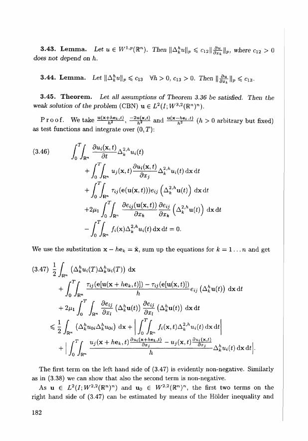
3.43. Lemma. Let u G W^(Rn). Then \\Ahu\\p ^ c 1 2 | | ^ - | | p . where c12 > 0 does not depend on h.
3.44. Lemma. Let \\Ahu\\p ^ c13 Vh > 0. c13 > 0. Then | |-^-| |p <C c13.
3.45. Theorem. Let all assumptions of Theorem 3.36 be satisfied. Then the weak solution of the problem (CBN) u G L2(I; JV3'2((Rn)n).
P r o o f . We take "(*+**»'), =^Q. a n d u(x-Aefc,t) ( / i > Q a r b i t r a r y b u t fixed)
as test functions and integrate over (0,T):
rT . + / / u J - ( x , 0 - " ^ E l - - A ^ u i ( . ) d x d «
JO JRW vXj
+ / / r i j (e(u(x ,<)) )e i i (A^u(<)) dxdt
+ */1^&K-<«>)<-* - / / / i (x )A^u i (< )dxd t = 0.
JO JRn
We use the substitution x — he^ = x, sum up the equations for k = 1 . . . n and get
(3.47) \ f ( A ^ i ( T ) A ^ ( T ) ) dx
^ JR"
+ / 7 ^ ( e [ u ( x + /xe f c , t ) ] ) - r i j ( e[u(x , t ) ] ) e i j ^
Jo Jun h
< i / (A£UO.A£U 0 . ) dx + / / /<(x, t )A^ f cu.(0dxdt -- JLRn I JO JRn I
+ / / ^ ^-AhUi(t)dxdt\. 1 JO JR™ h '
The first term on the left hand side of (3.47) is evidently non-negative. Similarly as in (3.38) we can show that also the second term is non-negative.
As u e L2(I;VV2'2((Rn)n) and u0 £ VV2'2((Rn)n, the first two terms on the right hand side of (3.47) can be estimated by means of the Holder inequality and
182

Lemma 3.43. The estimate of the convective term is a bit more complicated. It
follows from the Holder inequality and Lemma 3.42 that
Tf u^ + he^tf-^^-u^t)^^ II Jo Ju /o Jw- h
A%Ui(t)dxdt
I | u ( i ) l i 4 1 ( i ( U j ( M ) ^ r ) ) dx) d^using(3-31) <c8 f (f |u(i)|2|o(2)u(t)|2dx+ / |ou(t)|4dxV dt
Jo \JR» JR" J
^CsrOluWIIooluW^ + luWI2,,)^. JO
The first term is estimated by means of Lemma 3.18 and the apriori estimate in L2(I; VV2,2((Rn)n). The other term can be estimated by the following interpolation inequalities and imbeddings:
a) n = 3 1 3 1 3
Ml,4 < lull,2lUll,6 < lUll,2lUl24,2
and the boundedness follows from the estimate in L2(I; lV2,2(IRn)n); b) n = 2
l U | l ,4 ^ lu l?,2lU l2 ,2
(see e.g. [18]) and we use again the same apriori estimate as above. Thanks to
the Korn inequality we have that f0TJRri A£(I}(2I(u(£))A£(D(2 '(u(^ ^ cM which
together with Lemma 3.44 gives ||u||z,2(/.jy3,2(Rn)«) - ci4 . Moreover, the term
| fQ JRn Tij(e(u(x,t)))eij(A2k' u(t)) dxdt\ is uniformly bounded for arbitrary h > 0.
•
4. W E A K SOLUTION FOR THE MONOPOLAR FLUID
Hereafter we will study the problem (3.1)-(3.3), assuming fi^ —> 0 + . We denote by uN the solution of the problem (CBN) (i.e. with / / ^ ) , by u the solution of the problem (CMN) (i.e. with fix = 0). Our system of equations (for the monopolar fluid) takes the form
(4.1) ^ = 0 , OXi
(4.3) Mt(x,0) =u 0 t (x ) ,
183

where the tensor function r^(e) satisfies the conditions (1.6)-(1.10).
Using the apriori estimates in L°°(I; H) and LP(I; Vp) (only these do not depend
on /J,?) we can get thanks to the estimate of the time derivative in LP'(I; (X(Q)')
(X(Cl) = {<pe VV04'2(ft) n Wl*(ft) n W^'tfl); div<D = o} , n a bounded open sub
set of lRn) the existence of the measure-valued solution of the problem (CMN) for
p > ^ - . It means that there exists a couple (u,i/),
uGLP( I ;V p )nL°°( I ;H ) ,
veL~(QT;M(Un2))
2 2
(M(IRn ) is the space of the Radon measures on lRn ) such that
(4.4) J (-i^-u^^
= / wot^idx JR"
for every ip e Cl(I\ %(Rn)n), <D(T) = 0 and
(4.5) Du(x,t) = f Xdu(X) a.e. in QT. JR»2
In the case of the pertubated linear model (i.e. r(e) = (u0 + ^i |e |p"2)e for p < 2)
we get the same result as above for arbitrary p > 1 in both the two- and the three-dimensional case. This is connected with the fact that we have also an independent estimate in L2(J;V2)- For more detailed description see [16] or for the Dirichlet problem [2] or [11].
In the next part we will try to find new estimates of solution of the problem (CBN) which will make the limiting passage in the nonlinear term possible. So we will get a weak solution of the problem (CMN). In fact the estimates will guarantee that DuN ->» Du in Lp(I;Lp((Rn)n2), i.e. VuN -> Vu a.e. in QT. Then, using Lemma 2.9, we will get the desired limiting passage. About the data we will assume the following:
(4.6) u 0 € l V 1 ' 2 ( K n ) n n H ,
jL 2 ( I ;L 2 ( IR n ) n ) , p^2 f G ' \ L p ' ( I ; L p ' ( R n ) n ) , p<2,p' = ^ .
The weak solution of the problem (CMN) is defined as follows:
184

4.7. Definition. Let u0, f satisfy (4.6), and let p ^ 1 + ^ . Then a function u, where
(4.8) u e Lp(I; Vp) n C(I; H) n L2(I; W1»2(RB)n),
(4.9) ^ € L 2 ( / ; J f ) ,
is called a weak solution of the problem (CMN) if
(4.10) / -^<pidx+ / Uj^<pidx+ / Tij(e(u))eij(<p)dx= / fi<Pidx Jun at Jun axj Jun Jun
is satisfied a.e. in I for every <D G Vp n VV1'2(lRn)n.
4 .11 . Definition. Let u0 , f satisfy (4.6), and let p ^ ^ - . Then a function u,
where
(4.12) ue^^nn/jff),
is called a weak solution of the problem (CMN) if
(4.13) - / u^dxdt+ [ Uj~-<pidxdt+ f r i j(e(u))efj((D)dxdf JQT
at JQT
ax3 JQT
= / fiipidxdt+ / u0i<pi(0)dx JQT «!Rn
is satisfied for every <p e C1 (I; %(Un)n) with <p(T) = 0.
4.14. R e m a r k . The existence of a weak solution means that the Young measure
v from (4.4) is the Dirac measure a.e. in QT, i.e. v^,t = 6(X — Du(x, t)) for a.e. (x, t) G
QT-
Let u N be a solution of the problem (CBN), i.e. with fi? > 0. Let /if -> 0+ for N —> oo. From Chapter 3 we have the following apriori estimates, which do not depend on /LXI:
(4.15) | | u " | | L ~ ( / ; i 0 < c i ,
(4-16) I I - O ^ I I L P ^ L P C R - ) - - ) ^ ^ -
From Theorem 3.45 we know that uN is bounded in L2(I; W3>2(Rn)n) and therefore also in L2(I; W 1 ' 0 0 ^ * ) " ) (of course, the estimate tends to oo when -+ 0+). We want to use A u N as a test function in (3.9). However it is not possible to
185
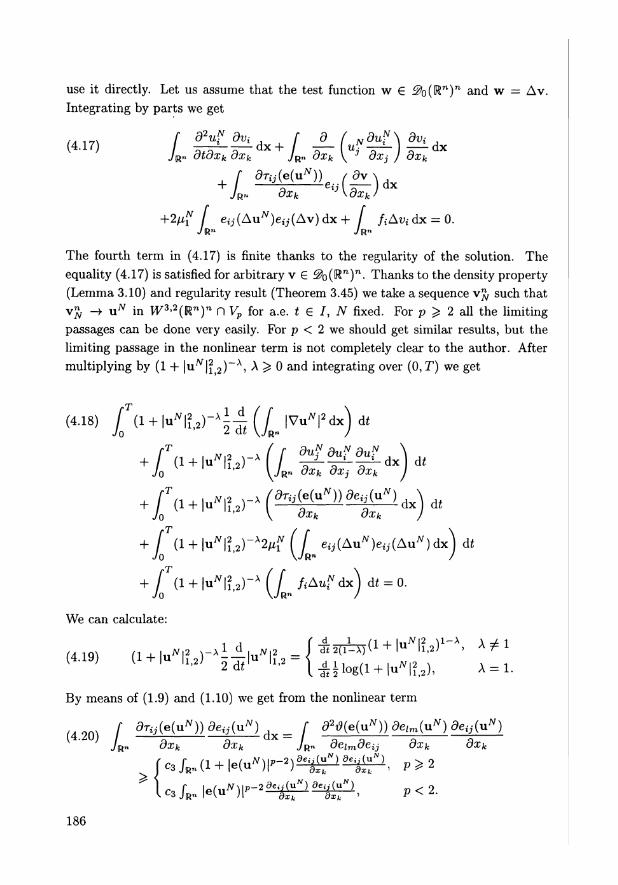
use it directly. Let us assume that the test function w e %(Un)n and w = Av. Integrating by parts we get
(4.17) f _ _ _ _ _ ! _ d x + / A ( > _ _ _ ) i__ d x jR» dtdxk dxk jRn dxk \ J dxj ) dxk
+ / _______) ej.f__.\dx JRn dx k
%J\dxk)
+2fiN f eij(AuN)eij(Av)dx+ f fiAvidx = 0. Jun Ju11
The fourth term in (4.17) is finite thanks to the regularity of the solution. The equality (4.17) is satisfied for arbitrary v E %(Un)n. Thanks to the density property (Lemma 3.10) and regularity result (Theorem 3.45) we take a sequence v ^ such that vft -> u N in Wz'2(Un)n fl Vp for a.e. t e I, N fixed. For p ^ 2 all the limiting passages can be done very easily. For p < 2 we should get similar results, but the limiting passage in the nonlinear term is not completely clear to the author. After multiplying by (1 + \uN\l2)~x, A ^ 0 and integrating over (0,T) we get
(4.18) ^ T ( l + | u " | ? i 2 ) - ^ Qf_ | V u " | 2 d x ) dt
+ | (l + \uN\l2)-x2vN (J^eij(AuN)eij(AuN)dx) dt
+ / (1 + | u " | ? i 2 ) - A (J fiAuNdx) dt = 0.
We can calculate:
(4.19) (l + | u " | ? i 2 ) - * ~ | u " | ? i 2 = 1 d , V i a í i 2 T í ^ ) ( l + l^lf,2)1-A. A#l
^ i l o g ( l + | u w | 2 , 2 ) , A = l . , N | 2 ^ A _ _ _ l u A t | 2 = j dt2(T=A)
2dť l 1 , 2 I -illne-n +111 1?
By means of (1.9) and (1.10) we get from the nonlinear term
(4 20) f ^ _ _ _ _ _ . _ _ _ _ _ _ d x = f dH(e(uN))delm(uN)deij(uN) jR™ dxk dxk jRn deimdeij dxk dxk
> (c3fRn(l + \e(uN)r*)detf)aet:N), P>2
*{c3JUn\e(uN)r>d<t:")detf\ P<2-
186

4.21. R e m a r k . For the perturbated linear problem we get on the right hand side of (4.20)
^ 0 + W o « ) r , ^ * ^ , > ,
We denote the term on the right hand side of (4.20) by ^ and
(4.22) (l + | u N | ? , 2 ) - V = ^ -
As the term with p^ is obviously non-negative, we can rewrite (4.18) as follows:
j j j i ^ d + I^PDfiJ^ + j f j r d .
< + c ( u o ) + / T ( i + | u " . ; i ! ) - > " i ! > 3 JO
(4.23)
,dŕ
+ / T (l + |uw£2Г л / ЛДufdx Jo JRП
dť
(for A = 1 the first terms on the left hand side is replaced by \ log(l + \uN\{ 2 ) ) .
4.24. R e m a r k . Using a similar technique as in Remark 3.34 we would obtain the same results for u 0 G H but only on [<S,T], 5 > 0 arbitrary. This remark holds for everything which will be proved in this chapter.
4.25. L e m m a . For u smooth enough we have
(4.26) \\D^u\\2^cA/l2 forp>2,
(4.27) | | 0 ( a ) u | | . , < C 5 | u | : * V - - forl<p<2.
P r o o f . The inequality (4.26) is a direct consequence of the Korn inequality and the definition of J?. The other one follows from the Holder and Korn inequalities:
H-jWull? < c / | % ^ P d x = c / f ^ ^ | e r A $ | e | ^ d x JUn I OXk JR« \oxk 0Xk J
^cý\ | e | p d x )
„ (2-í0.>
^ ^ Ч u | 1 ) P
2 •
D
4.28. R e m a r k . For the perturbated linear model we get that the inequality
(4.26) is satisfied for p > 1.
187

The forcing term can be now estimated by means of (4.26) (for p ^ 2) or (4.27) (for p < 2). Let us demonstrate this in the latter case.
From (4.21) and the Young inequality it follows that
dt (4.29) / (l + | u " | ? i 2 ) -* / / . A u f d x JO JR"
^ [T(l + \uN\l2)-*\\f\\p,\\DWuN\\pdt Jo
^ c5 f s*\*N& a+|uw|1)2)-*nfnP-(i+|uw|li2)-^ Jo
< e / Xdt + c(e) / T ( l + |u w | ? , 2 ) - A | | f | | ^ |u w | ? - p dt . Jo Jo
The first term is transferred to the left hand side of (4.23) with a small coefficient while the second term can be estimated by means of the Holder inequality:
(4.30) jf nf|i2,|u|2-pd^ (jT iifiijdtj " (jf l u x * ) "
- HfIIL*''(/;LV(R»)»)llU H^(/;Vr) ^ C( f) '
We obtain
dí (4-31) 5 - [ i _ ( i + , u N ( r ) | ? i a ) i - A + | ^ ^
T
< c ( u o , f ) + / (l + |uw | ? i 2)-A |uw | ? i 3dt . Jo
Now it remains to estimate the convective term on the right hand side of (4.31). If we get such an estimate with A ^ 1 then we have from the first term on the left hand side of (4.31) that u e L°°(I; W^2(Rn)n) and consequently from the other term (if p ^ 2) we obtain our desired estimate in L2(I; VV2,2(lRn)n). For A > 1 we have only fQ Jjf dt -$ const.
Hereafter, we will write only u instead of uN. We will deal with the problem for n = 3 and at the end we will only give a sketch of the proof for n = 2.
a. Cauchy problem in 3 space dimensions.
4.32. Lemma. For u smooth enough we have
(4.33) \u\lt3p ^ce^i.
188

Proof.
M«i:,-/4(v(wi))'d.</.M-"^^*.<^.
the inequality (4.33) follows from the imbedding VV 1 ' 2^ 3 ) 3 «-> L6(R3)3 and the Korn
inequality. •
We will solve separately two cases:
(i) P > 3 (li) 1 < p < 3
ad i) p ^ 3
Put A = 0. Prom Lemmas 3.16 and 4.25 we see that |u|ff2 ^ c | | u | | 2 < / i . The
interpolation inequality
(4-34) Ks^HjpMf?
and the Young inequality yield
f \u\l3dt^cf Nlp^-S-Vlulg Jo Jo
rp rp
f J?dt + c(e)f |u|0dí. Jo Jo
5ÍЄ
The first term is transferred to the left hand side of (4.31), the other is finite because
-^Y ^ 1 for p > 3.
ad ii) 1 < p < 3
Considering the fact that 2 < 3 < 3p and p < 3 < 3p for p G (1,3) we can use the
following interpolation inequalities:
- i
(4-35) luks Hj Hf--;, м—1 3-y
(4-36) |u|i,s < | u | 1 ) P | u | 1 ) 3 p .
Prom (4.33) we get
(4.37) | u | 3
) 3 ( l + K , 2 ) - * = \u\3^+1~a\l + | u | ? ) 2 ) - A
^ c 7 ^ « M u | ^ ( i + H ? ) 2 ) - ^ 3 - - ^ - - ,
where Qt = 3^~°> + 3a?=f, Q2 = 3a£ f i . Integrating (4.37) over (0,T) we obtain
£ |u|3 ,3(l + |u|? ) 2)-* dt < c7 j T X* |u|«» (1 + | u | ? ) 2 ) - A + 3 - - ^ - - + ^ dt.
189

We claim
(4.39) -A + 3 ( p - 1 ) ( 1 - Q )
+ A o . 1 = 0 . op — z
Using the Holder and Young inequalities under the assumptions Q\6 = 1, $2^' = P
and j -f- jr = 1 we get
(4.40) J \u\l3(l + \u\l2)-"dt^c(J Xdt)\JQ K p d t ) " .
From (4.16) and (4.40) it follows by means of the Young inequality
(4-41) 2(l^A)(1 + | u ( : r ) l ? ' 2 ) 1 ~ A + 5 4 j ( ^ d < ^ c ( u ° ' f ) -
It remains to find the values of a, A, 6, 6' and verify whether their values are in
the required intervals. Solving the above mentioned system of equations we find
(4.42) a = ^ - 5 )
(4.43) Л = 2
6 ( p - l ) '
3 - P З p - 5 '
Hence a G [0,1] <=> p G [§, 3] and A ^ 0 <=> p G (§, 3]. Moreover, A ^ 1 <=i> p ^ n 5
^-. We can also verify that 6 and 0"' > 1.
4.44. R e m a r k . In the case of the perturbated linear model we can use the
interpolation of VV1'3(Rn) between VV1'2(Rn) and VV1'6(Rn) and then, thanks to the
imbedding of VV2'2(Rn) <-* TV1 , 6(Rn), we can estimate the convective term by means
of a similar technique as above for A = 2(3 — p), i.e. A ^ 0 Vp > 1.
As A ^ 1 for p ^ ~ we get the following lemma:
4.45. Lemma. Let p ^ -g- and let UQ, f satisfy (4.6). Then the sequence of 11 5
solutions of the problem (CBN) for u.^ -> 0 + is uniformly bounded in the following
norms:
(4.46) | | U N | | L ~ ( / ; W - . - Ҷ R З ) 3 ) ^ C 5 ,
(4.47) | | U І V | | L Ҷ / ; W 2 . 2 ( R З ) 3 ) ^ Cв,
(4.48) Ц U ^ І І L I Ҷ / Î W ^ З I Ҷ R 3 ) 3 ) < c 7-
190
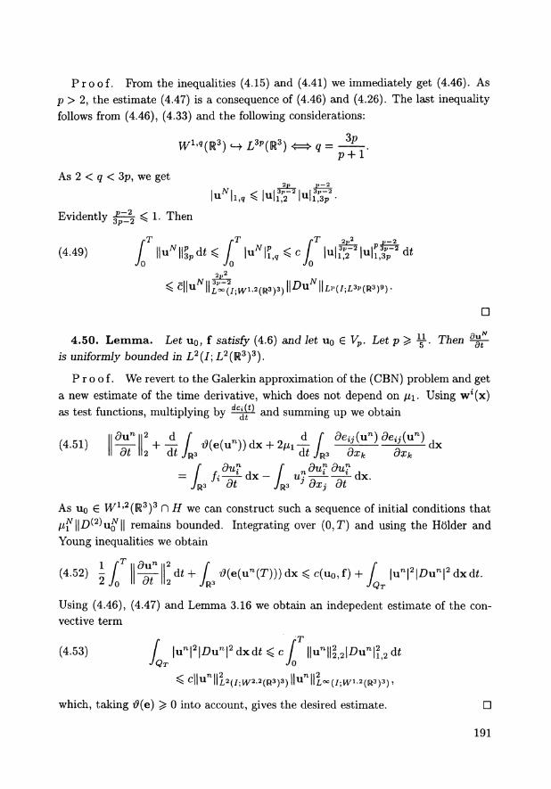
P r o o f . From the inequalities (4.15) and (4.41) we immediately get (4.46). As p > 2, the estimate (4.47) is a consequence of (4.46) and (4.26). The last inequality follows from (4.46), (4.33) and the following considerations:
W^q(U3) «-> L3p(U3) <=>q= - ^ y .
As 2 < q < 3p, we get
| u N | i , , < | u | ^ | u | g .
Evidently f ^ ^ 1. Then
rrt rri rri Q
(4.49) f \\nN\\lpAt^f | u X W | u | g ^ | u | ^ d t Jo Jo Jo
2„2
< C | | U N | | ^ 2/ ; W 1 , 2 ( R 3 ) 3 ) | | - D U N | | L P ( / ; L 3 P ( R 3 ) 9 ) .
D
4.50. Lemma. Let u0, f satisfy (4.6) and let u0 G Vp. Let p ^ ^ . Then -~^-is uniformly bounded in L2(I; L2(IR3)3).
P r o o f . We revert to the Galerkin approximation of the (CBN) problem and get
a new estimate of the time derivative, which does not depend on Lti. Using w l(x)
as test functions, multiplying by Ctdy and summing up we obtain
(„,, i £ i \ A / ,(e(„.„dx+2, * I y >»«<«•>,. <9* 2 d£ JR3 d£ JR3 a.xfc dxk
f ,duf. f ndu?du? = / ^ ^ T d x " / u j 7 T ^ ^ r d x -JR3 dt JR3
j ctej dt
As u0 G VV1,2((R3)3 n H we can construct such a sequence of initial conditions that ^jv | |£)(2)u^|| remains bounded. Integrating over (0,T) and using the Holder and Young inequalities we obtain
1 CT II d u n i i2 C f
<4-52) o b i T d * + / ^(e(u n (T)))dx^c(u 0 , f ) - f - / |un |2 |L>un |2dxd*. 2 J0 II dt 112 JR3 JQT
Using (4.46), (4.47) and Lemma 3.16 we obtain an indepedent estimate of the con-vective term
(4.53) / | u n | 2 | L > u n | 2 d x d ^ c / ||un||252|.Dun|2
)2dt JQT JO
^ ClluTl||L2(/;iy2.2(IR3)3) l l U n | |L~(/ ; iyL2( R 3)3) ,
which, taking 17(e) ^ 0 into account, gives the desired estimate. •
191

4.54. Theorem. Let u0, f satisfy (4.6) and let u0 G Vp. Letp ^ -^. Then there exists a unique weak solution of the problem (CMN) in the sense of Definition 4.7. Moreover, the solution is regular, i.e. u G L°°(I; KV1,2(IR3)3) n L2(I; VV2'2((R3)3) n
P r o o f . Existence. The same method as in Lemma 3.10 gives that there exists a countable subset of %(U3)3 which is dense in KVlj2((R3)3 n Vp. Similarly as in Theorem 3.36 we get a "diagonal" subsequence such that for arbitrary R positive DuN' -> Du in L2(I;L2(BR)9), i.e. DuN' -> DuN a.e. in I x BR. Using Lemma 2.9 we get
(4.55) / -r-^Wiipdxdt + / Uj-^-Wiipdxdt + / Tij(e(u))eij(w)ipdxdt JQT
dt JQT
dxJ JQT
fiW^dxdt Vi/> G C°°(I),Vw G %(U3)3. -L QT
Similarly as in Theorem 3.36 we will prove that (4.55) is satisfied for all w G 1^1,2,^3)3 n Vp a n d a e i n (QTy
Let w be an arbitrary function from W 1 ' 2 ^ 3 ) 3 n Vp, w n G ^ 0 ( -^ 3 ) 3 , w n -» w (i.e. w n + w in VV1'2((R3)3 and Vw n -> Vw in LP(U3)9). Then, thanks to the estimates from Lemmas 4.45 and 4.50 we get that (4.55) is satisfied for all w G w1>2(M3)3nvp.
To complete the existence part of the proof we must verify that u G C(I; II). This can be done in the same way as in Theorem 3.36. We get again that u 6 C - ( / ; f f ) .
Uniqueness. It will be proved similarly as for the (CBN) problem. Let u, v be two different solutions, w = u — v . Using w as a test function in (4.10) we obtain
(4-56) ^ l l w l l l + f3(Tij(e(u)) - rij(e(v)))eij(w)dx = J wj-^-Widx.
In the same way as in the uniqueness part of Theorem 3.36 we can prove
f f f1 d2dOL
/ (rij(e(u))-Tij(e(v)))eij('w)dx^ / / e»j(w)efc<(w) d a d x JR3 JR3 J0 oeijOeki
with tfa = d(e[v + a(u - v)]). However, (1.10), the Korn inequality and the fact that p > 2 imply
c|w|?2 . (4.57) / (r{j(e(u)) - r i j(e(v)))e i j(w)dx > JR3
Integrating (4.56) over (0,£), using (4.57) and w(0) = 0 we obtain
(4.58) | | |w( t ) | | i + c j f |w|2,2dt = £ | |w| | j |u | l l 2dt.
192

1 1
Prom the interpolation inequality ||w||4 - ||w||-f ||w||£, the imbedding Wl>2(U3)
<-+ L6(U3) and the apriori estimate of u in L°°(I; VV1'2(R3)3) we get
(4.59) \\w(t)\\l<c f ^ T ^ d r . Jo
Then the Gronwall inequality gives ||w(£)||2 = 0 a.e. in I, i.e. u = v a.e. in QT- •
4.60. R e m a r k . When u0 $. Vp, we do not have the information about the
time derivative from Lemma 4.50. Nevertheless we can get the estimate of the time
derivative in L2(I; (VV2'2((Rn)n n Vp)') which implies (see [5 pp. 147-149]) that u
belongs to C(I; H). So we get the existence (and uniqueness) of the weak solution of
the problem (CMN). However we have to assume (4.13) instead of (4.10) with test
functions <p 6 L2(I; Vp n Wx>2(Un)n) with §£ G L2(I; L2(Un)n).
Now we will deal with the case p < ^-, separately for p ^ 2 and p < 2.
ad a) p ^ 2
We can dispose only with
CT 3-(4.61) / (l + | u | ? 2 ) - 2 3 p * , / d t < const.
do
4.62. Lemma. Let (4.61), (4.15) and (4.16) hold. Then J^ \\D^u\\2/ ^ c7
th f3 = |H=| for p > 2, p = \ forp = 2.
P r o o f . For some ft < 1 (which will be specified later) we have
(4.62) Í \\DWn\\¥ d< < c4 í jl>(l + | u | 2 , 2 ) - 2 ^ ( l + |u|2 3 ) 2 ě - V át
JO Jo
šc(£jTát) ( ^ ( l + Hull-HD^u)!!)3^^)1 ,
where Lemma 3.16 was used. As we know that u is bounded in L°°(I;H) we can put
3 - P /? 2/3 = 2
Зp-51-ß
and get /? = f^zf • Now we use the Young inequality and transfer the term
e J0 ||-D(2)u||2/3d£ with e sufficiently small to the left hand side. For p = 2 we can
use directly the estimate in L2(I;V2) and get 2§5|y~0 = 1> ie- P = | - D
193

Let us note that (3 G (0, | ) for p G (2, -^) .
Thanks to the apriori estimates we have
rp
(4.64) / | |u Jo
т 2(3 < Гa 2,2 ^ C 8 -
0
Using the imbedding PV2'2(IR3) <-> PV i+^IR 3 ) which holds for s = - ^ (i.e. s G
(if ,1] for p G [2,-g-) ) we see that £ | |u | | 2 £ s p ^ c9. We choose g G (l ,p) . Let
a G (0,5) (which will be specified later). The interpolation inequality (2.4) implies
(4.65) l |u| |i+tT ,p<c||u| |l;- | |«| |f+ , i I ,
and therefore
(4-66) j T ||u||?+<r,p < c j T | | u | | £ - - ^lullg,,,,
where \ 4- ^- = 1. Both terms on the right hand side are bounded when
(4.67) g ( l - - j ) j = P>
</-<*' = 2/3.
(/rj llullpd* < °° because of the imbedding VV1'P(IR3) <--> L ^ ( ( R 3 ) and the interpo
lation between L2(1R3) and L^( IR 3 ) . )
Solving the system (4.67) we get
(4.68) «=S-{p-f/-V ' q P~2(3
We can also verify that $, 5' > 1. So we have
4.69. Theorem. Let u0, f satisfy (4.6) and let p G [2, ^-) . Then there exists
a weak solution u of the problem (CMN) in the sense of Definition 4.11. Moreover,
u G Lq(I; VV1+CT'P(IR3)), where <? G (l,p) and a satisfy (4.68).
P r o o f . Let u ^ be our bounded sequence in Lq{I\ IV1+cr'p(IR3)3). Because of the estimate of the time derivative mentioned at the beginning of this chapter we get from the Lions-Aubin Lemma that uN -> u in L9(I; VV1 '9^)3) , where fi is an
194

arbitrary bounded open subset of R3. We use again the technique of the "diagonal"
subsequence. From Theorem 2.9 we get for (p e Cl(I; %(U3)3), <p(T) = 0
(4.70) - / Ui-^dxdt+ Uj^(pidxdt+ / ^(etuJJeyOp) dxd* JQT
d t JQT
dxo JQT
= / fnpidxdt+ / uoi<Pi(0)dx. JQT Jun
D
4.71. R e m a r k . We can try to close the test functions in Cl(I; VpnTV1»2(R3)3).
(We know that %(U3)3 is dense in Vp n IV 1 ' 2 (R 3 ) 3 .) We would have to assume that
\T\ ^ c | e | p _ 1 in order to control the nonlinear term.
ad b) p < 2
Now let p < 2. We can make use only of (4.61) and the apriori estimates (4.15)
and (4.16). Using (4.27) (Lemma 4.25) we see that
(4.72) / | u | 2 , p K - 2 ( l - f | u | 2 , 2 ) - 2 ^ d ^ const. Jo
fT
/o
For some /? < 1 we calculate
(4.73) / \\DЄ>u\\lßdt J0
< [ (HІ>IГP
2(1 + \"\ҺГ2Щß Ийa_p)(i + Hh)2ß^ dt
( / 3 ) / T | u | 2 , p K - 2 ( l + | u | 2 , 2 ) - 2 ^ d í Jo
+є(ß) / ű P ( i + H 2 , 2 ) 2 ^^dí. Jo
rT
/o
Using the interpolation inequality
5 P - 6 3 ( 2 - ľ ) 2V (4-74) | u | l l 3 ^ | u | , £ |n|1 %_
1 ' 3 - ,
and the imbedding VV1'P(R3) <-> L ^ ( R 3 ) we see that the second term in (4.73) is bounded by
(4-75) /TM?>l&d.+ / V l i ! / ^ do do
195

with Q, = (2-p + 2%fX6)) A and g 2 = e ^ ^ i ^ . T h e second term in (4.75) is finite if 0 ^ f. The first term can be estimated by means of the Young inequality
(4.76) £ |u |ft |u|& dt^e [T \u\ff dt + c(e) £ |u|ft*. JO Jo Jo
The first integral is transferred to the left hand side of (4.73) and the other is
5 + 8' finite when the following holds (\ + j? = 1):
(4.77) Q2S' = 2/3
Qi S = p.
Solving (4.77) we get
(4.78) p(5p - 9)
P 2 ( -p 2 + 8p - 9)
and therefore /3 £ (0, | ) for p £ ( | , 2). We get tha t p must be greater t han | instead of | , which was the bound from the estimate of the convective term. The case p = | must be excluded . Evidently, the condition (3 < § is satisfied as well as <5, 6' > 1 . Prom (4.16) and the above proved estimate we see tha t
(4.79) ГïïDuft J0
T
p < ClO 0
with p satisfying (4.78). Let us choose a £ (0,1) . More precisely, a must satisfy (4.83) as will be seen later.
Thanks to the interpolation inequality (2.5) we get ||Du||<-.)P -$ c||Z)u||J>p | |i.)u||p~cr. Let q > 1. Then
(4.80) [T \\Du\\ltP ^ c f \\Dn\\^\\Dn\\p1-^ dt
Jo Jo
< ( £ \\Du\\°f dt) T ( £ \\Du\\^-"^ dt) '.
Solving the system ( \ + jr = 1)
(4.81) aqS' = 20
(1 - e)qS = p
196

we obtain
23p (4.82) q= PP
ap + 2/3(1 -oУ
where a must satisfy
(4.83) ff<ÍP-l)(5p-9) p(з - p)
Therefore we have
4.84. Theorem. Let p > | , Jet u0, f satisfy (4.6). Then there exists a weak
solution of the problem (CMN) in the sense of Definition 4.11.
P r o o f . It is analogous to the proof of Theorem 4.69. •
4.85. R e m a r k . It is possible to close the test function in Cl(I;Vp) but only
for p ^ 3 + Y 3 9 This bound follows from the estimate of the convective term.
When we assume the perturbated linear model, i.e. with r(e) = (i/0 + ^ i | e | p _ 2 ) e
for p < 2, we can get the existence of a weak solution for all p > 1. As we have the
estimate of the convective term for p > 1 we can get by means of a similar technique
as above that J0 | |Du||2^, - c with /? = y r ^ a r-d therefore we have
4.86. Theorem. Let p > 1, let u0, f satisfy (4.6) and r(e) = (i/0 + i/ i | e | p - 2 )e .
Then there exists at ieast one weak solution of the problem (CMN) in the sense of
Definition 4.11.
b. Sketch of the proof in 2 space dimensions.
First we will estimate the convective term in (4.31). As for p ^ 3 the proof is
completely analogous to the three-dimensional case, we will deal separately with two
cases:
(i) 2 ^ p < 3
(ii) p < 2
ad i) 2 < p < 3
4.87. Lemma. Let p € [2,3). Then for u smooth enough we have
(4-88) K , 3 < c | u | f ) 2 ( ^ i + | | u | | l ( / i ) ,
(4-89) |u|?,3 < c | < p (J*-? + H u l l ^ ^ 2 ^ ) .
197

P r o o f . VV3'2(IR2) <-> L3(IR2), which together the interpolation inequality 2 I
||Vu|| i 2 ^ c||u| | | ||u||i 2 and Lemma 3.16 gives the first inequality.
The other one follows from the imbedding W2^,P(U2) <-> L3(IR2), the interpola-, £
3--v (Ì = 4--v
A = = 3-- P ,
tion inequality | | V u | | 2 3 ^ p <: c||Vu||^ ||Vu||23p , the imbedding IV1'2((R2) *-•> Wv*,
(4.26) and Lemma 3.16. " D
Now we can apply Lemma 4.87 to the convective term and we get, similarly as in the three-dimensional case, the following system of equations ( \ -f- jr = 1):
(4.90) -A + a + A a + ( 1-2a ) ( 3-p )=o
a + (l-a)(3-p)f
2 <5 = 1
p(l — a ^ ' = p.
Solving the system (4.90) we obtain
(4.91)
(4.92)
i.e. a € (0, | ] and A - 1 for p £ [2,3). We can also verify that o~, 8' > 1.
ad ii) 1 < p < 2
4.93. Lemma. Let p G [f, 2). Then we have for u smooth enough
(4.94) |u|?i3 c\n\f^\u\f^J^,
(4.95) K , 3 < c K i P £ / ^ .
Proo f . As VV1'P(IR2) M- Z^-r(OS2) and (4.21) hold, the first inequality is a
consequence of the interpolation inequality |u|f 3 ^ | u | i ( 2 _ 1 ) | u | *(VJ^ • X ' 2 - P
The other one follows from by same argument and the interpolation inequality 5p-G 2 ( 3 - p )
,F i ' 2 - ; >
198

Now we will apply the previous lemma to the convective term and get the following
- + ---system of equations ( i + -*r = 1):
QS = 1
(-£#•-)'->• Solving the above mentioned system we get
2 ( p - l ) ( 3 - p ) (4.97)
(4.98)
5p — 6 3 - p
P - 1 7
i.e. a e ( | , 1] for p € [§, 2), A > 1 for p < 2. We can also verify that <5, 5' > 1.
4.99. R e m a r k . For the perturbated linear model we can make use of (4.88) and 4.95. This enables us to estimate the convective term with A = 2 '3~p ' for p > 1.
Now we revert to the case when p ^ 2 , i.e. A ^ l . Similarly as in three space dimensions we get
4 .100. Lemma. Let uN be solutions of the problem (CBN) with jjiN > 0.
pN —> 0+. Let p ^ 2. Then uN are unifromly bounded in the following norms:
(4-101) ||UN||L~(/;W-.2(R2)2) ^ Cn,
(4.102) ||U7V||L2(/;V1/2,2(R2)2) ^Cl2,
(4.103) ||uN||L,>(/;wi.j>(R2)2) -$ci3.
4 .104. Theorem. Let u0.f satisfy (4.6) and u0 G Vp. Let p ^ 2. Then there exists a unique weak solution of the problem (CMN) in the sense of Definition 4.7. Moreover, the solution is regular, i.e. u G L°°(I; IV1'2(IR2)2) n L2(I; VV2'2((R2)2).
P r o o f . The proof is analogous to the proof of Theorem 4.54 and Lemma 4.50. Only in the uniqueness part we use ||u||4 - 2* ||u||f |u|f 2 (see [17]). D
199

Now let us solve the case when p < 2, i.e. p £ [§, 2). We can make use only of
(4.105) / (l + | u | f 2 ) - ^ c / d ^ const Jo
together with (4.15) and (4.17). From (4.105) and (4.27) we get
(4.106) / M l > l i ~ 2 ( l + | < a ) - K * dt ^ const . Jo
For ft < 1 (which will be specified later) we get from the interpolation inequality
Mi,2 < M i ^ M x l L ^ t h e imbedding W ^ R 2 ) *-> L^(R2) analogously to
the three-dimensional case
(4.107) / \\D^u\\2/dt^c14
Jo
with
(4.108) / ?= P ( 2 P " 3 )
( P - 1 ) ( 6 - P )
The case p = | must be excluded again.
4.109. Theorem. Let u0. f satisfy (4.6), p > §. Then there exists a weak solution of the problem (CMN) in the sense of Definition 4.11.
P r o o f . It is completely analogous to the proof of Theorems 4.84 and 4.69
including the part between (4.79) and (4.83). D
4.HO. R e m a r k . It is possible to close the test functions in Cl(I\ Vv) for p ^ 1 - y ^ . This bound follows again from the estimate of the convective term.
For the perturbated linear problem we can get thanks to the estimate of the convective term similarly as above the following theorem:
4.111. Theorem. Let u0, f satisfy (4.6). Then there exists at least one weak
solution of the problem (CMN) in the sense of Definition 4.11.
Acknowledgement . I would like to thank Jindfich Necas and Josef Malek for
several helpful discussions.
200

[1 [2:
[з:
к [5
[e:
t<: P:
[9
[ю:
[ii:
[12:
[iз: [14
[15:
[ie:
[i<:
[is:
[19: [20
References
R. A. Adams: Sobolev Spaces. Academic Press, 1975.
H. Bellout, F. Bloom, J. Nečas: Young Measure-Valued Solutions for Non-Newtonian Incompressible Fluids . P r e p r i n t , 1991. H. Bellout, F. Bloom, J. Nečas: Phenomenological Behaviour of Mult ipolar Viscous Fluids . Q u a t e r l y of Applied M a t h e m a t i c s 54 (1992), no. 3, 559-584. M. E. Bogovskij: Solutions of Some Prob lems of Vector Analysis with t h e O p e r a t o r s div a n d grad. T r u d y Sem. S. L. Soboleva (1980), 5-41. (In Russian.) N Dunford, J. T. Schwarz: Linear O p e r a t o r s : P a r t I. General Theory . Interscience Publ i shers I n c , New York, 1958. H. Gajewski, K. Gröger, K. Zacharias: Nichtl ineare Operatorgle ichungen u n d Opera-tordifferentialgleichungen. Akademie Verlag, Berlin, 1974. J. Kurzweil: O r d i n a r y Differential Equat ions . Elsevier, 1986. O. A. Ladyzhenskaya: T h e M a t h e m a t i c a l Theory of Viscous Flow. G o r d o n a n d Beach, New York, 1969. D. Leigh: Nonlinear C o n t i n u u m Mechanics. McGraw-Нill, New Yoгk, 1968. J. L. Lions: Qeulques mé thodes de résolution des problèms aux limites non lineaires. Dunod , Paris , 1969. J. Málek, J. Nečas, A. Novotný: Measure-valued solutions a n d a s y m p t o t i c behavior of a mult ipolar model of a b o u n d a r y layer. Czech. M a t h . Ј o u r n a l Ą2 (1992), no. 3, 549-575. J. Málek, J. Nečas, M. Rűzička: О n Non-Newtonian Incompressible Fluids. MЗAS 1
(1993).
J. Nečas: An I n t r o d u c t i o n t o Nonlinear Elliptic Equat ions . Ј . Wiley, 1984.
J. Nečas: T h e o r y of Mult ipolar Viscous Fluids. T h e m a t h e m a t i c s of finite e lements a n d appl icat ions VII, M A F E L A P 1990 (Ј . R. W h i t e m a n , ed.) . Academic Press, 1991, p p . 233-244. J. Nečas, M. Šilhavý: Mult ipolar Viscous Fluids. Quater ly of Applied M a t h e m a t i c s 49 (1991), no. 2, 247-266. M. Pokorný: Cauchy Pгoblem for t h e Non-Newtonian Incompressible Fluid (Master degree thesis, Facul ty of M a t h e m a t i c s a n d Physics, Charles University, P r a g u e . 1993. K. R. Rajagopal: Mechanics of Non-Newtonian Fluids. G. P . Galdi, Ј . Nečas: Recent Developments in Theoret ica l Fluid Dynamics . P i t m a n Research Notes in M a t h . Series 291, 1993. R. Temam: Navier-Stokes E q u a t i o n s — T h e o r y a n d Numerical Analysis. N o r t h Holland, A m s t e r o d a m - N e w York-Оxford, 1979. H. Triebel: Theory of Funct ion Spaces. Birkhäuser Verlag, Leipzig, 1983. H. Triebel: In terpola t ion Theory, Funct ion Spaces, Differential Оpera tor s . Verlag der Wiss., Berlin, 1978.
Author's address: Milan Pokorný, Faculty of Science of Palacký University, D e p a r t m e n t of Ma themat i ca l Analysis and Numerical Mathemat ics , Tomkova 40, 772 00 Olomouc, Czech Republ ic (e-mail p o k o r n y Q r i s c . u p o l . c z ) .
201