Int j simul model 12 (2013) 4, 225-236 ISSN 1726-4529 Original scientific paper

DOI:10.2507/IJSIMM12(4)2.241 225

USE OF NEURAL NETWORKS IN PREDICTION

AND SIMULATION OF STEEL SURFACE ROUGHNESS

Saric, T.; Simunovic, G. & Simunovic, K. University of Osijek, Mechanical Engineering Faculty in Slavonski Brod, Trg I. Brlic-Mazuranic 2,

HR – 35000 Slavonski Brod, Croatia E-Mail: tsaric@sfsb.hr

Abstract Researches on machined surface roughness prediction in the face milling process of steel are presented in the paper. The data for modelling by the application of neural networks have been collected by the central composite design of experiment. Input variables are the parameters of machining (number of revolutions – cutting speed, feed and depth of cut) and the way of cooling, while the machined surface roughness is output variable. In the modelling process the algorithms Back-Propagation Neural Network, Modular Neural Network and Radial Basis Function Neural Network have been used. Various architectures of neural networks have been investigated on a data sample and they have generated the prediction results which are at the RMS (Root Mean Square) error level of 5.24 % in the learning phase (8.53 % in the validation phase) for the Radial Basis Function Neural Network, 6.02 % in the learning phase (8.87 % in the validation phase) for the Modular Neural Network and for the Back-Propagation Neural Network 6.46 % in the learning phase (7.75 % in the validation phase). (Received in September 2012, accepted in June 2013. This paper was with the authors 3 months for 2 revisions.) Key Words: Neural Networks, Surface Roughness, Face Milling, Modelling and Simulation 1. INTRODUCTION The transfer of new technological knowledge into own production systems, the inventiveness of those working in the preparation and production as well as the application of new scientific approaches that will improve the level of knowledge and organization in production preparation sectors have a considerable impact upon the final characteristics of products. The essential characteristic of a product or of the parts built into the product is the required quality of the machined surfaces, very often demonstrated by the surface roughness. It has a crucial influence on technological time and overall production costs but on fatigue resistance, lubrication, friction, and wear properties as well [1-2]. The surface roughness is affected by many controlled and uncontrolled process parameters that are difficult to achieve and continuously monitor. Controlled parameters of a machining process are feed rate, depth of cut and cutting speed. Other factors, such as the material properties of tool and workpiece, workpiece quality, tool geometry, cutting conditions, type of workpiece clamping, tool machine vibrations, tool wear etc. cannot be easily controlled [3-11]. On this basis, the aim of many scientific-research projects and scientific papers is to model, simulate and predict the surface roughness and optimize cutting parameters to obtain the desired level of surface quality of machined products. In the field of modelling and roughness prediction neural networks (NN) are widely applied. The authors first conduct designed experiments. The Taguchi design of experiment is often used to reduce the time and cost of the experiments [12, 13], but the central composite [14] and the full factorial design of experiments [1] are also used. The main purpose of designed experiments is to monitor the

Saric, Simunovic, Simunovic: Use of Neural Networks in Prediction and Simulation of …

226

influence of controlled parameters on surface roughness [1, 15-18], but some authors also add other parameters like chip’s characteristics [12], pre-tool wear vibrations [19], workpiece-tool vibration [20], lubrication-cooling condition [21] etc. For modelling and later for predicting the surface roughness different NN are used: Radial Basis Function NN, Feed Forward NN, Bayesian NN and Neuro-Fuzzy networks. El-Sonbaty et al. [19] predicted the surface roughness using a Feed Forward Back- Propagation NN with different structures. The roughness prediction error of obtained model is about 2 %. NN based on Back-Propagation learning algorithm is used to develop the surface roughness model in paper [22]. The roughness prediction model proved applicable with an error of about 3 %. Feed Forward Back-Propagation was selected in paper [23], and in defining the model various transfer functions were compared. Munoz-Escalona et al. [12], developed different types of NN (Radial Base Feed Forward and Generalized Regression) which evaluated surface roughness following face milling. The best results were achieved by the Feed Forward NN. The investigation also showed that the surface roughness was most affected by the chip thickness and cutting speed. In the roughness prediction model developing different techniques are often combined: Fuzzy Logic and NN, NN and Harmony Search algorithm (HS) [24], NN based on 2D Fourier transform [25] and others. The intention is to define quality models based on a small set of data [26] and to reduce error in roughness prediction within the limits from 1.5 to 10 %. The purpose of this paper is to investigate and compare the influence of different algorithms i.e. architectures of NN on error degree of the roughness prediction model of the steel surface machined by face milling. Three NN algorithms have been used (Back-Propagation Neural Network - BPNN, Modular Neural Network - MNN and Radial Basis Function Neural Network - RBFNN). 2. DEFINITION OF PROBLEM AND RESEARCHING GOAL The data set was obtained based on the conducted central composite design of experiment with the position of the axial runs from the centre of experiment, which amounts to 1 [27]. Input variables were the machining parameters (number of revolutions – cutting speed, feed and depth of cut) and the way of cooling (without cooling, cooling through the tool and cooling outside the tool). Factor levels are shown in Table I.

Table I: Factor levels data.

Factor Factor name Low level Medium level High level A Depth of cut, mm 0.5 1 1.5 B Feed, mm/min 100 300 500 C Number of revolutions, min-1 400 600 800

D Way of cooling without cooling through the tool cooling

cooling outside the tool

Specimens used in experiment were made from S235JRG2 structural steel plates; dimensions 100×70×20 mm. Measuring specimens were prepared in advance. The surfaces planned for milling were premachined and to obtain equal clamping side faces of the specimens were also machined. The milling process was performed by an angle milling head of 80 mm diameter, of producer ISCAR (cutting plates H490 ANKX). The machining device was a vertical CNC milling machine MAG FTV 850-1800. The output variable i.e. surface roughness Ra, was measured according to the standard and required measuring procedures, using the device Talysurf Surtronic duo by Taylor Hobson. Measured roughness was within

Saric, Simunovic, Simunovic: Use of Neural Networks in Prediction and Simulation of …

227

limits 0.33-2.95 m. A representative number of specimens and measuring data were provided by the design of experiment while the broad spectrum complexity of cases provided a good sample for NN training and testing. Distribution of type entries by separate specimens i.e. sub-specimens was performed out of the initial set of data according to the principle of coincidence. After that the set was divided into three classes with the limits (widths) of the classes adjusted so as to have equal number of types (i.e. observed cases) in each class. This was done so that each of the three classes could have the same number of cases and that some classes would not be given preference in the NN learning process. The model variables which were not numerical had to be transformed into categories and classes (way of cooling).

2.1 Selection of the type of neural networks – general models

The abstract mathematical description of an artificial neuron (Fig. 1a) is derived based on the imitation of the functions of a biological neuron.

a)

b)

Figure 1: a) Neuron structure; b) Back-Propagation Neural Network.

Table II: Some graphs and expressions of transfer functions.

Graph of transfer function Expression of transfer function

Line

ar

5,0if05,05,0if

5,0if1

i

ii

i

i

InputInputinput

InputOutput

Sigm

oid

iInputGi eOutput

1

1

Sinu

s

ii InputGOutput sin

Hyp

erbo

lic-

tang

ent

ii

ii

InputGInputG

InputGInputG

i eeeeOutput

Saric, Simunovic, Simunovic: Use of Neural Networks in Prediction and Simulation of …

228

As can be seen from Fig. 1a the neuron body takes over the role of a summator while the role of dendrites is taken over by the inputs to the summator. The biological neuron activation level of sensitivity is taken over by the transfer-activation function which determines the moment of launching the impulse to the neuron output. The transfer function can be linear or nonlinear (Table II). In linear transfer functions the summator output is multiplied by the factor and the amount thus obtained is forwarded to the neuron output. In nonlinear functions the summator outputs change in accordance with various forms of functions while the neuron outputs can take over different values depending on transfer function. G is the function increment. It is calculated as G = 1/T. T is the function threshold. Along with the transfer functions given in Table II the transfer function Digital Neural Network Architecture – DNNA is also used in the investigation. The character of DNNA is nonlinear and is calculated according to the Eq. (1). The transfer function output (xi) uses the input signal – vector (oj) to connect with the weights (wij) in the interval [0, 1] and can be mathematically expressed as:

j

jiji owx )1(1 (1)

In most applications it is important for the transfer functions to be able to accept negative signals and weights. If these signals and weights are to be separated and their activation values taken as positive and negative values, they are given through the values of the variables: xi

+ i xi-, and computed by the following expressions:

0

)1(1jij ow

jiji owx (2)

0

)1(1jij ow

jiji owx (3)

As there are no corresponding postulates defining which kinds of transfer functions could be allocated to which kinds of problems, it follows that the choice should be made on a concrete problem in the phase of defining the corresponding architecture of a NN. Learning rules (algorithms) make it possible to adjust (calculate) the weights of the connections between neurons. There are a number of learning rules but the following ones have been chosen for this investigation: Delta rule (generalized Delta rule), Delta-Bar-Delta, Extended Delta-Bar-Delta and Normalised-Cumulative Delta rule. For most real problems different rates of learning are used for different layers with a low level of the learning rate for the output layer. During learning on a defined structure of neural network it is necessary to define and accept the criteria to evaluate the level of success of this process. Quantification of these criteria serves to compare the applied algorithm with other algorithms used for learning. For the proposed investigation Root Mean Square error – RMS was adopted:

N

OdMSRMS

N

nnn

1

2)( (4)

where: MS – Mean Square error; dn – Desired value of a NN nth output; On – NN nth output; N – Number of pairs of the training set input-output values.

Back-Propagation Neural Network represents an important technique to define nonlinear transfer functions between continuous input values and one or more output values. Every layer is completely connected with the following one thus indicating a great number of synapses. Fig. 1b displays the BPNN standard structure. To better understand the computation

Saric, Simunovic, Simunovic: Use of Neural Networks in Prediction and Simulation of …

229

of the values in the network (Fig. 1a, b) and to avoid confusion from the neuron in one layer to the other layer the indices and exponents will be used to describe the characteristic attributes. They are given in what follows:

sjx – output state of the jth neuron in the sth layer, sjiw – weight of the connection of the ith neuron in the (s-1) layer with the jth neuron in the

sth layer, sjI – weighted sum of input of the jth neuron in the sth layer.

At the start of the learning process i.e. of the connections' weights computation, the input layer transfers data to the first hidden layer. Every neuron in the hidden layer receives the weighted input which is, by the network initialization, usually given random values in the interval from -0.1 to 0.1. These inputs are transformed in view of the previously defined attributes and get the form:

n

i

si

sji

sj xwI

1

1 (5)

The computed neuron inputs are transformed through the transfer or activation function and sent to the output of the neuron according to the following expression:

sj

i

si

sji

sj Ifxwfx

1 (6)

where f is the transfer function (sigmoid or some other selected function). Every sending of the neuron output is connected with a local error. Let's suppose now that the network has some global error of the function E connected with the differential of the function of all the connections' weights in the network. The global error E is defined in the output layer and is given as:

25.0 kk xdE (7)

where: dk is the desired (real) output, while xk presents the output of the network and k is the index of the output component. The critical parameter that represents the error and propagates backwards through all the layers of the network is defined as:

sj

sj I

Ee

(8)

Using connected rules twice successively the relation is obtained between the local error and the particular neuron of the sth layer and all local errors of the layer s+1, given by the expression:

k

skj

sk

sj

sj weIfe 11' (9)

The previous expression can be used only for non-output layers. The aim of the learning process i.e. of adjusting the connection weights in this network is to minimize global error and propagate it backward through the network all the way to the input layer. The aim of this propagation of the minimized global error through the network is to adjust every particular connection weight in the network. According to the set of current values of the weights s

jiw ascent or descent is defined, the aim being the global error reduction. This can be realized by applying the gradient descent rule:

s

ji

sji w

Ew (10)

Saric, Simunovic, Simunovic: Use of Neural Networks in Prediction and Simulation of …

230

where is the learning coefficient. Partial derivations in the above expression can be calculated directly from the local error value, which is given by the following expression:

1

si

sjs

j

sj

sj

sji

xewI

IE

wE (11)

Including the calculated values of partial derivations from Eq. (11) into the Eq. (10) the expression for adjusting the weights is obtained:

1 si

sj

sji xew (12)

One of the problems of the descent algorithm is the setting of the corresponding learning coefficient. The change of the weights as a linear function of partial derivations (defined in Eq. (10)) forms the assumption that the surface error is locally linear where the adjective locally is defined by the magnitude of the coefficient of learning. If the curvature of the point is sharp the assumption of linearity does not hold and divergence will appear close to this point. That is why the coefficient of learning should be kept at a low level. On the other hand a small coefficient of learning can result in very slow learning. To solve such diametrically opposed demands the notion of momentum is introduced. The expression for the weight increment given in Eq. (12) is changed in such a way that added to it is the product of the factors of the weight increment and the momentum, given by the following expression:

sji

si

sj

sji wmomentumxew 1 (13)

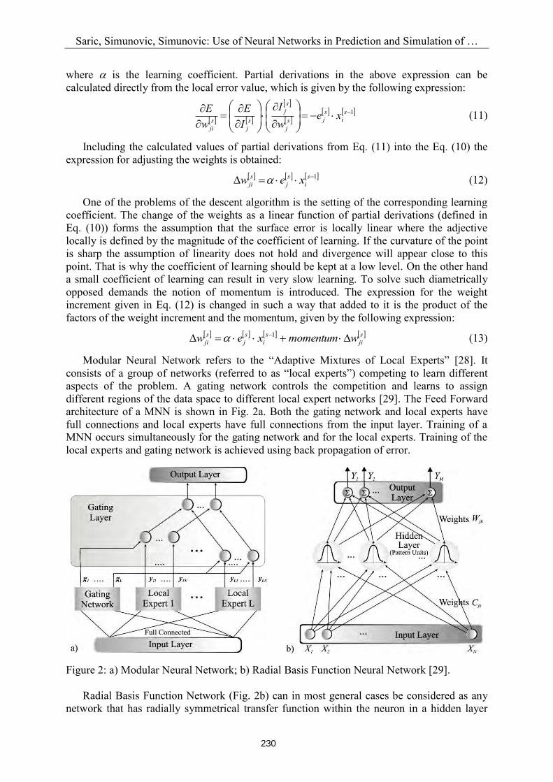
Modular Neural Network refers to the “Adaptive Mixtures of Local Experts” [28]. It consists of a group of networks (referred to as “local experts”) competing to learn different aspects of the problem. A gating network controls the competition and learns to assign different regions of the data space to different local expert networks [29]. The Feed Forward architecture of a MNN is shown in Fig. 2a. Both the gating network and local experts have full connections and local experts have full connections from the input layer. Training of a MNN occurs simultaneously for the gating network and for the local experts. Training of the local experts and gating network is achieved using back propagation of error.

Figure 2: a) Modular Neural Network; b) Radial Basis Function Neural Network [29]. Radial Basis Function Network (Fig. 2b) can in most general cases be considered as any network that has radially symmetrical transfer function within the neuron in a hidden layer

Saric, Simunovic, Simunovic: Use of Neural Networks in Prediction and Simulation of …

231

(samples layer). For the sample unit (hidden layer neuron) to be radially symmetric it must have the three following elements: Centre, the input domain vector usually saved in the output layer weights vector in the sample unit; Measurements of distance, the measures which define the distance of the input vector from the centre; it is usually the standard Euclidian measure of distance; Transfer function, the function of a single variable. It defines the output of the neuron with functional mapping of the distance from the centre. The common transfer function is the Gaussian function which intensifies output values of variables when the distance is small. The Gaussian function parameter of width for the kth unit of the hidden layer sample is calculated by the following expression:

P

Pkpkk cc

P 1

21 (14)

where: P is the value determined heuristically for the method of the closest neighbours; given a cluster centre ck, let k1,..., kp be the indices of the P nearest neighbouring cluster centres (internally P = 2). As previously described when computing global error of a learning set, the learning algorithm will be able to adjust the connection weights. The global error in an output layer is calculated using the following expression:

2

121

N

iii YdE (15)

where: di is calculated output value of the network; Yi is desired output value of the sample i; N is number of samples in the learning set.

3. EXPERIMENTAL RESULTS AND DISCUSSION

3.1 Results obtained by Back-Propagation Neural Network

After analyzing and summing up the results in Table III, obtained in the investigation using various architectures of BPNN, it can be seen that the best result was obtained by the combination of the Sigmoid transfer function and the Delta rules of learning. Further analysis of results led to the conclusion that the best results were obtained by the Sigmoid transfer function for the BPNN.

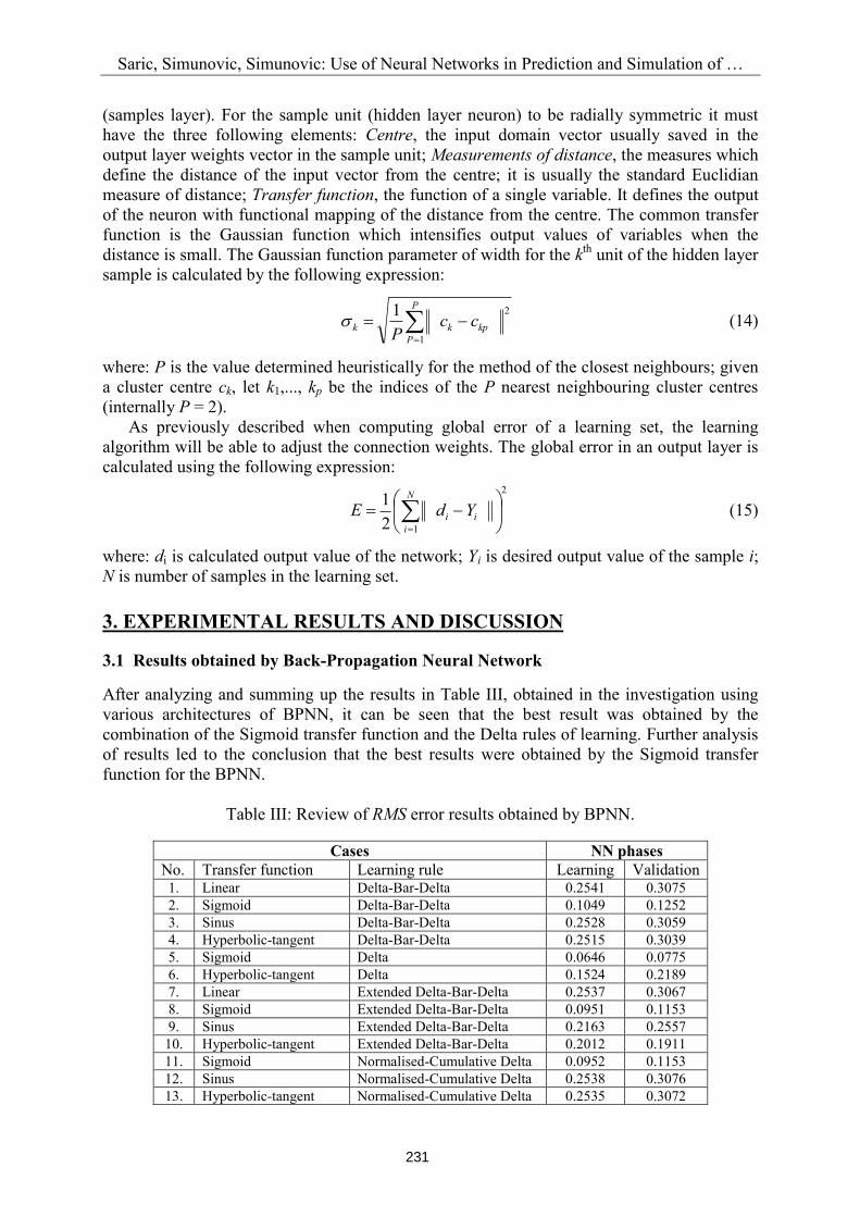
Table III: Review of RMS error results obtained by BPNN.

Cases NN phases No. Transfer function Learning rule Learning Validation 1. Linear Delta-Bar-Delta 0.2541 0.3075 2. Sigmoid Delta-Bar-Delta 0.1049 0.1252 3. Sinus Delta-Bar-Delta 0.2528 0.3059 4. Hyperbolic-tangent Delta-Bar-Delta 0.2515 0.3039 5. Sigmoid Delta 0.0646 0.0775 6. Hyperbolic-tangent Delta 0.1524 0.2189 7. Linear Extended Delta-Bar-Delta 0.2537 0.3067 8. Sigmoid Extended Delta-Bar-Delta 0.0951 0.1153 9. Sinus Extended Delta-Bar-Delta 0.2163 0.2557 10. Hyperbolic-tangent Extended Delta-Bar-Delta 0.2012 0.1911 11. Sigmoid Normalised-Cumulative Delta 0.0952 0.1153 12. Sinus Normalised-Cumulative Delta 0.2538 0.3076 13. Hyperbolic-tangent Normalised-Cumulative Delta 0.2535 0.3072

Saric, Simunovic, Simunovic: Use of Neural Networks in Prediction and Simulation of …

232

The next transfer function with the best result was the Hyperbolic-tangent one. Better results of the Sigmoid function were to be expected as it was defined (Table II) for positive values while the Hyperbolic-tangent function was defined for both positive and negative values. Our data model for inputs and outputs consisted exclusively of the positive values of the model variables. Fig. 3a shows parallel values of the surface roughness obtained by measuring in the conducted experiment on a machine during the machining process and predictive values based on the model obtained by the BPNN.

3.2 Results obtained by Modular Neural Network

Applications of the MNN on the data set and the obtained results are given in Table IV. The architecture with the combination of the Sigmoid transfer function and the Delta rules of learning produced the RMS error lowest level of 6.02 %. The Sigmoid transfer function in combination with the Extended Delta-Bar-Delta, the Delta-Bar-Delta and the Normalized-Cumulative Delta rule of learning, with the corresponding architectures, produced the RMS error lowest levels.

Table IV: Review of RMS error results obtained by MNN.

Cases NN phases No. Transfer function Learning rule Learning Validation

1. Linear Delta-Bar-Delta 0.2438 0.2911 2. Sigmoid Delta-Bar-Delta 0.0972 0.1225 3. Sinus Delta-Bar-Delta 0.2374 0.2933 4. Hyperbolic-tangent Delta-Bar-Delta 0.2347 0.2920 5 Sigmoid Delta 0.0602 0.0887 6. Hyperbolic-tangent Delta 0.1670 0.2241 7. DNNA Delta 0.0615 0.0820 8. Linear Extended Delta-Bar-Delta 0.1853 0.1888 9. Sigmoid Extended Delta-Bar-Delta 0.0776 0.0903 10. Sinus Extended Delta-Bar-Delta 0.1555 0.2030 11. Hyperbolic-tangent Extended Delta-Bar-Delta 0.1515 0.1936 12. DNNA Extended Delta-Bar-Delta 0.0643 0.0846 13. Sigmoid Normalised-Cumulative Delta 0.0950 0.1148 14. Hyperbolic-tangent Normalised-Cumulative Delta 0.1577 0.2344 15. DNNA Normalised-Cumulative Delta 0.0681 0.0872

Figure 3: Roughness prediction by the application of: a) BPNN; b) MNN. Further analysis shows that the DNNA transfer function produces the lowest dissipation of output results (within 1 %) and after the Sigmoid function it can be accepted for the MNN application. Fig. 3b displays graphical representation of the model predicted results of the

Saric, Simunovic, Simunovic: Use of Neural Networks in Prediction and Simulation of …

233

surface roughness and the real (actual) values obtained by the experiment. Thus the obtained result proves the theory that says the results obtained by the MNN are usually better than the results of the BPNN. 3.3 Results obtained by Radial Basis Function Neural Network

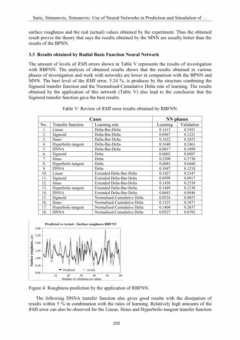
The amount of levels of RMS errors shown in Table V represents the results of investigation with RBFNN. The analysis of obtained results shows that the results obtained in various phases of investigation and work with networks are lower in comparison with the BPNN and MNN. The best level of the RMS error, 5.24 %, is produces by the structure combining the Sigmoid transfer function and the Normalised-Cumulative Delta rule of learning. The results obtained by the application of this network (Table V) also lead to the conclusion that the Sigmoid transfer function gave the best results.

Table V: Review of RMS error results obtained by RBFNN.

Cases NN phases No. Transfer function Learning rule Learning Validation

1. Linear Delta-Bar-Delta 0.1613 0.2451 2. Sigmoid Delta-Bar-Delta 0.0967 0.1221 3. Sinus Delta-Bar-Delta 0.1622 0.2453 4. Hyperbolic-tangent Delta-Bar-Delta 0.1640 0.2461 5. DNNA Delta-Bar-Delta 0.0817 0.1098 6. Sigmoid Delta 0.0602 0.0887 7. Sinus Delta 0.2300 0.3730 8. Hyperbolic-tangent Delta 0.6083 0.6660 9. DNNA Delta 0.1047 0.1218

10. Linear Extended Delta-Bar-Delta 0.1427 0.2347 11. Sigmoid Extended Delta-Bar-Delta 0.0599 0.0917 12. Sinus Extended Delta-Bar-Delta 0.1438 0.2339 13. Hyperbolic-tangent Extended Delta-Bar-Delta 0.1449 0.2338 14. DNNA Extended Delta-Bar-Delta 0.0643 0.0846 15. Sigmoid Normalised-Cumulative Delta 0.0524 0.0853 16. Sinus Normalised-Cumulative Delta 0.1525 0.2471 17. Hyperbolic-tangent Normalised-Cumulative Delta 0.1404 0.2037 18. DNNA Normalised-Cumulative Delta 0.0527 0.0782

Figure 4: Roughness prediction by the application of RBFNN. The following DNNA transfer function also gives good results with the dissipation of results within 5 % in combination with the rules of learning. Relatively high amounts of the RMS error can also be observed for the Linear, Sinus and Hyperbolic-tangent transfer function

Saric, Simunovic, Simunovic: Use of Neural Networks in Prediction and Simulation of …

234

in combination with different rules of learning (except for the combination with the Delta rule of learning), up to 23 %. Fig. 4 presents the results obtained by measuring in the process of machining and calculating with the best architecture of the RBFNN. 3.4 Review of the best results

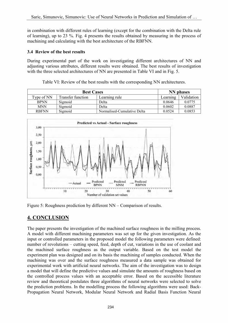
During experimental part of the work on investigating different architectures of NN and adjusting various attributes, different results were obtained. The best results of investigation with the three selected architectures of NN are presented in Table VI and in Fig. 5.

Table VI: Review of the best results with the corresponding NN architectures.

Best Cases NN phases Type of NN Transfer function Learning rule Learning Validation

BPNN Sigmoid Delta 0.0646 0.0775 MNN Sigmoid Delta 0.0602 0.0887

RBFNN Sigmoid Normalised-Cumulative Delta 0.0524 0.0853

Figure 5: Roughness prediction by different NN – Comparison of results. 4. CONCLUSION The paper presents the investigation of the machined surface roughness in the milling process. A model with different machining parameters was set up for the given investigation. As the input or controlled parameters in the proposed model the following parameters were defined: number of revolutions – cutting speed, feed, depth of cut, variations in the use of coolant and the machined surface roughness as the output variable. Based on the test model the experiment plan was designed and on its basis the machining of samples conducted. When the machining was over and the surface roughness measured a data sample was obtained for experimental work with artificial neural networks. The aim of the investigation was to design a model that will define the predictive values and simulate the amounts of roughness based on the controlled process values with an acceptable error. Based on the accessible literature review and theoretical postulates three algorithms of neural networks were selected to solve the prediction problems. In the modelling process the following algorithms were used: Back-Propagation Neural Network, Modular Neural Network and Radial Basis Function Neural

Saric, Simunovic, Simunovic: Use of Neural Networks in Prediction and Simulation of …

235

Network. In the experimental process and the investigation of the proposed model, different architectures of neural networks were modelled. On the modelled architectures the attributes were adjusted and various transfer functions and learning rules investigated. On the modelled architectures of neural networks the learning process and the testing on the proposed data sample were conducted. The results obtained in the investigation are presented in tables, separately for every neural network algorithm. The different architectures of neural networks, investigated on the data sample, generated the best prediction results which are at the level of the RMS (Root Mean Square) error of 5.24 % in the learning phase (8.53 % in the validation phase) for the Radial Basis Function Neural Network, 6.02 % (8.87 % in the validation phase) for the Modular Neural Network and Back-Propagation Neural Network 6.46 % (7.75 % in the validation phase). The results obtained in the investigation and the levels of the RMS error are acceptable in view of the proposed technological model for roughness prediction. The modelled algorithms of neural networks could be implemented and efficiently used as a part of a technological module or within the information systems used as a support to the planning and modelling of technological processes. REFERENCES [1] Öktem, H. (2009). An integrated study of surface roughness for modelling and optimization of

cutting parameters during end milling operation, International Journal of Advanced Manufacturing Technology, Vol. 43, No. 9-10, 852-861, doi:10.1007/s00170-008-1763-3

[2] Al-Zubaidi, S.; Ghani, J. A.; Che Haron, C. H. (2011). Application of ANN in Milling Process: a Review, Modelling and Simulation in Engineering, Vol. 2011, Article ID 696275, 7 pages, doi:10.1155/2011/696275

[3] Stampfer, M. (2009). Automated setup and fixture planning system for box-shaped parts, International Journal of Advanced Manufacturing Technology, Vol. 45, No. 5-6, 540-552, doi:10.1007/s00170-009-1983-1

[4] Brezocnik, M.; Buchmeister, B.; Gusel, L. (2011). Evolutionary Algorithm Approaches to Modeling of Flow Stress, Materials and Manufacturing Processes, Vol. 26, No. 3, 501-507, doi:10.1080/10426914.2010.523914

[5] Tadic, B.; Jeremic, B.; Todorovic, P.; Vukelic, D.; Proso, U.; Mandic, V.; Budak, I. (2012). Efficient workpiece clamping by indenting cone-shaped elements, International Journal of Precision Engineering and Manufacturing, Vol. 13, No. 10, 1725-1735, doi:10.1007/s12541-012-0227-8

[6] Gusel, L.; Rudolf, R.; Romcevic, N.; Buchmeister, B. (2012). Genetic programming approach for modelling of tensile strength of cold drawn material, Optoelectronics and Advanced Materials –Rapid Communications, Vol. 6, No. 3-4, 446-450

[7] Antic, A.; Petrovic, P. B.; Zeljkovic, M.; Kosec, B.; Hodolic, J. (2012). The Influence of Tool Wear on the Chip-Forming Mechanism and Tool Vibrations, Materiali in tehnologije, Vol. 46, No. 3, 279-285

[8] Stankovic, I.; Perinic, M.; Jurkovic, Z.; Mandic, V.; Maricic, S. (2012). Usage of Neural Network for the Prediction of Surface Roughness after the Roller Burnishing, Metalurgija, Vol. 51, No. 2, 207-210

[9] Cosic, P.; Lisjak, D.; Antolic, D. (2010). The iterative multiobjective method in optimization process planning, Tehnicki vjesnik – Technical Gazette, Vol. 17, No. 1, 75-81

[10] Leo Dev Wins, K.; Varadarajan, A. S. (2012). Simulation of surface milling of hardened AISI4340 steel with minimal fluid application using artificial neural network, Advances in Production Engineering & Management, Vol. 7, No. 1, 51-60

[11] Wang, J.-C.; Chen, C.-H.; Lee, B.-Y. (2012). The design model of micro end-mills made by using the Finite Element Method, Transactions of FAMENA, Vol. 36, No. 2, 41-50

[12] Munoz-Escalona, P.; Maropoulos, P. G. (2010). Artificial Neural Networks for Surface Roughness Prediction when Face Milling Al 7075-T7351, Journal of Materials Engineering and Performance, Vol. 19, No. 2, 185-193, doi:10.1007/s11665-009-9452-4

Saric, Simunovic, Simunovic: Use of Neural Networks in Prediction and Simulation of …

236

[13] Elhami, S.; Razfar, M. R.; Farahnakian, M.; Rasti, A. (2013). Application of GONNS to predict constrained optimum surface roughness in face milling of high-silicon austenitic stainless steel, International Journal of Advanced Manufacturing Technology, Vol. 66, No. 5-8, 975-986, doi:10.1007/s00170-012-4382-y

[14] Simunovic, K.; Simunovic, G.; Saric, T. (2013). Statistical modelling of surface roughness of aluminium alloy and brass alloy, Materialwissenschaft und Werkstofftechnik, Vol. 44, No. 7, 618-625, doi:10.1002/mawe.201300061

[15] Samanta, B.; Erevelles, W.; Omurtag, Y. (2008). Prediction of workpiece surface roughness using soft computing, Proceedings of the Institution of Mechanical Engineers, Part B: Journal of Engineering Manufacture, Vol. 222, No. 10, 1221-1232, doi:10.1243/09544054JEM1035

[16] Bajic, D.; Lela, B.; Zivkovic, D. (2008). Modeling of machined surface roughness and optimization of cutting parameters in face milling, Metalurgija, Vol. 47, No. 4, 331-334

[17] Lela, B.; Bajic, D.; Jozic, S. (2009). Regression analysis, support vector machines, and Bayesian neural network approaches to modeling surface roughness in face milling, International Journal of Advanced Manufacturing Technology, Vol. 42, No. 11-12, 1082-1088, doi:10.1007/s00170-008-1678-z

[18] Mahdavinejad, R. A.; Khani, N.; Fakhrabadi, M. M. S. (2012). Optimization of milling parameters using artificial neural network and artificial immune system, Journal of Mechanical Science and Technology, Vol. 26, No. 12, 4097-4104, doi:10.1007/s12206-012-0882-9

[19] El-Sonbaty, I. A.; Khashaba, U. A.; Selmy, A. I.; Ali, A. I. (2008). Prediction of surface roughness profiles for milled surfaces using an artificial neural network and fractal geometry approach, Journal of Materials Processing Technology, Vol. 200, No. 1-3, 271-278, doi:10.1016/j.jmatprotec.2007.09.006

[20] Samanta, B. (2009). Surface roughness prediction in machining using soft computing, International Journal of Computer Integrated Manufacturing, Vol. 22, No. 3, 257-266, doi:10.1080/09511920802287138

[21] Bruni, C.; d’Apolito, L.; Forcellese, A.; Gabrielli, F.; Simoncini, M. (2008). Surface roughness modelling in finish face milling under MQL and dry cutting conditions, International Journal of Material Forming, Vol. 1, No. 1 Supplement, 503-506, doi:10.1007/s12289-008-0151-8

[22] Zain, A. M.; Haron, H.; Qasem, S. N.; Sharif, S. (2012). Regression and ANN models for estimating minimum value of machining performance, Applied Mathematical Modelling, Vol. 36, No. 4, 1477-1492, doi:10.1016/j.apm.2011.09.035

[23] Zain, A. M.; Haron, H.; Sharif, S. (2010). Prediction of surface roughness in the end milling machining using artificial neural network, Expert Systems with Applications, Vol. 37, No. 2, 1755-1768, doi:10.1016/j.eswa.2009.07.033

[24] Razfar, M. R.; Zinati, R. F.; Haghshenas, M. (2011). Optimum surface roughness prediction in face milling by using neural network and harmony search algorithm, International Journal of Advanced Manufacturing Technology, Vol. 52, No. 5-8, 487-495, doi:10.1007/s00170-010- 2757-5

[25] Palani, S.; Natarajan, U. (2011). Prediction of surface roughness in CNC end milling by machine vision system using artificial neural network based on 2D Fourier transform, International Journal of Advanced Manufacturing Technology, Vol. 54, No. 9-12, 1033-1042, doi:10.1007/ s00170-010-3018-3

[26] Grzenda, M.; Bustillo, A.; Quintana, G.; Ciurana, J. (2012). Improvement of surface roughness models for face milling operations through dimensionality reduction, Integrated Computer-Aided Engineering, Vol. 19, No. 2, 179-197, doi:10.3233/ICA-2012-0398

[27] Montgomery, D. C. (2009). Design and Analysis of Experiment, John Wiley and Sons, Hoboken [28] Jacobs, R. A.; Jordan, M. I.; Nowlan, S. J.; Hinton, G. E. (1991). Adaptive mixtures of local

experts, Neural Computation, Vol. 3, No. 1, 79-87, doi:10.1162/neco.1991.3.1.79 [29] NeuralWare. (2001). Neural Computing: A Technology Handbook for NeuralWorks Professional

II/Plus, NeuralWare, Aspen Technology, Pittsburgh