applying relation algebra and relview to measures in a - hal-shs

HAL Id: halshs-00355699https://halshs.archives-ouvertes.fr/halshs-00355699

Submitted on 23 Jan 2009

HAL is a multi-disciplinary open accessarchive for the deposit and dissemination of sci-entific research documents, whether they are pub-lished or not. The documents may come fromteaching and research institutions in France orabroad, or from public or private research centers.

L’archive ouverte pluridisciplinaire HAL, estdestinée au dépôt et à la diffusion de documentsscientifiques de niveau recherche, publiés ou non,émanant des établissements d’enseignement et derecherche français ou étrangers, des laboratoirespublics ou privés.

Applying Relation Algebra and RelView to Measures inaSocial Network

Rudolf Berghammer, Agnieszka Rusinowska, Harrie De Swart

To cite this version:Rudolf Berghammer, Agnieszka Rusinowska, Harrie De Swart. Applying Relation Algebra andRelView to Measures in aSocial Network. Working Paper GATE 2009-02. 2009. <halshs-00355699>

https://halshs.archives-ouvertes.fr/halshs-00355699

https://hal.archives-ouvertes.fr

Groupe d’An

ÉcUMR

DOCUMENTS DE TRAVAI

W.P. 0

Applying Relation Algebra anSocial N

Rudolf Berghammer, Agnieszka

Janvier

GATE Groupe d’Analyse etUMR 5824 d

93 chemin des Mouilles –B.P. 167 – 69131

Tél. +33 (0)4 72 86 60 60 – Messagerie électroniqu

Serveur Web : ww

GATE alyse et de Théorie

onomique 5824 du CNRS

L - WORKING PAPERS

9-02

d RelView to Measures in a etwork

Rusinowska, Harrie de Swart

2009

de Théorie Économique u CNRS

69130 Écully – France Écully Cedex Fax +33 (0)4 72 86 60 90 e [email protected]

mailto:[email protected]

Applying Relation Algebra and RelView to Measures in a Social

Network⋆

Rudolf Berghammer1, Agnieszka Rusinowska2 and Harrie de Swart3

1 Institut fur InformatikChristian-Albrechts-Universitat Kiel

Olshausenstraße 40, 24098 Kiel, [email protected]

2 GATEUniversite Lumiere Lyon 2 - CNRS

93 Chemin des Mouilles - B.P. 167, 69131 Ecully Cedex, [email protected]

3 Department of PhilosophyTilburg University

P.O. Box 90153, 5000 LE Tilburg, The [email protected]

Abstract. We present an application of relation algebra to measure players’ ‘strength’ in a socialnetwork with influence between players. In particular, we deal with power, success, and influence ofa player as measured by the Hoede-Bakker index, its generalization and modifications, and by theinfluence indices. We also apply relation algebra to determine followers of a coalition and the kernel ofan influence function. This leads to specifications, which can be executed with the help of the BDD-based tool RelView after a simple translation into the tool’s programming language. As an examplewe consider the present Dutch parliament.

Keywords: RelView, relation algebra, social network, the Hoede-Bakker index, influence index,follower, kernel

Corresponding author: Agnieszka Rusinowska

1 Introduction

In order to measure players’ (or agents’) ‘strength’ in a voting situation, a lot of power indices havebeen proposed in the course of more than fifty years (see, for instance, [1, 12, 13, 14, 18, 26, 27, 28,29, 35, 36, 46], see also [20, 31, 33, 48] for an extensive analysis of most of the power indices). Inthe voting power literature, one may find theoretical analysis (which includes both the axiomaticand probabilistic approaches to power indices) as well as applications of power indices (especiallyto decision-making in the European Union and the national parliaments).

Coming from a different direction is an approach proposed in [25], where a social networkwith players who are to make a ‘yes’-‘no’ decision is considered. In this framework, a decisionalpower (the Hoede-Bakker) index has been introduced. The essential feature of this framework isthe distinction between the inclination of a player (to say ‘yes’ or ‘no’) and the final decision of theplayer, which can be different from his initial inclination, due to influences of others in the network.Such an influence is formally represented by an influence function. The Hoede-Bakker index has beenrecently studied in [40, 41, 42, 43]. In [42] the authors introduce and investigate a generalization andsome modifications of the Hoede-Bakker index in a social network that coincide with some standardpower indices, like the Penrose measure (also called the absolute or non-normalized Banzhaf index),

⋆ Co-operation for this paper is supported by European Science Foundation EUROCORES Programme - LogICCC.

2 Rudolf Berghammer, Agnieszka Rusinowska and Harrie de Swart

the Coleman indices, and the Konig-Brauninger index. Moreover, ‘Success’, ‘Luck’, ‘Failure’ and‘Decisiveness’ of a player in a social network with influence between players were defined (foran analysis of success and decisiveness of a player in voting situations, see e.g. [30]). As shownin [40, 42], the generalized Hoede-Bakker index measures a kind of ’net Success’, i.e., ‘Success -Failure’, but if all inclination vectors are equally probable, this index coincides with the measureof ‘Decisiveness’.

Although the Hoede-Bakker index has been defined in the framework of influence, in fact itdoes not measure the influence between players. Influence indices, influence functions, and someother concepts related to influence (like the concepts of follower of a coalition, and of kernel of aninfluence function) have been investigated in [21, 22, 23, 24].

Since more than two decades, relation algebra is used successfully for formal problem specifi-cation, prototyping, and algorithm development, see e.g., [11, 47, 49]. Relations are well suited formodeling and reasoning about many discrete structures (like graphs, games, Petri nets, orders andlattices) and, due to the easy and/or efficient mechanization using, for instance, Boolean matrices,successor lists or binary decision diagrams (BDDs), also for computations on them. RelView (see[4, 2, 9]) is a BDD-based tool for the visualization and manipulation of relations and for prototypingand relational programming. In [7, 8, 45] relation algebra and RelView have been successfully ap-plied to compute the set of all feasible stable governments in a coalition formation model introducedin [44]. In the present paper we like to apply the same approach, but now to calculate measuresof parties’ ‘strength’ in a social network. Determining such measures can become quite complexand requires a lot of computations. Hence, using a computer program to calculate the measuresis extremely useful for real life applications of the concepts in question. To be more precise, theaim of this paper is to apply relation algebra and RelView to compute the Hoede-Bakker index,its modifications, and the influence indices, and to determine the followers of a coalition and thekernel of an influence function.

The structure of the paper is the following. Section 2 introduces the framework of influenceand measures of players’ strength in a social network. In Section 3 we present the facts on relationalgebra that are necessary to deliver the relation-algebraic specifications and algorithms of the keyconcepts of Section 2. In this section we also briefly describe the RelView tool. How to translatethe concepts of Section 2 into relation-algebraic specifications and RelView-code is demonstratedin Section 4. In order to illustrate the usefulness of the approach applied in this paper, we presentin Section 5 an example based on the real structure of the present Dutch Parliament. Doing so,we also refer to the concepts of dominant and central players. Finally, we present some concludingremarks in Section 6.

2 Measures of Players’ ‘Strength’ in a Social Network

The framework studied in the paper is the following. We consider a social network with the setof all players (voters) denoted by P := {1, ..., n}. The players make a certain acceptance-rejectiondecision. Each player has an inclination either to say ‘yes’ (denoted by 1) or ‘no’ (denoted by 0). ABoolean inclination vector, denoted by i = (i1, ..., in), indicates the inclinations of all players. Allinclination vectors are assumed to be equally probable. Let I := {0, 1}n be the set of all inclinationvectors. It is assumed that players may influence each other, and due to the influences in thenetwork, the final decision of a player may be different from his original inclination. In other words,each inclination vector i ∈ I is transformed into a decision vector Bi, where B : I → I with i 7→ Biis the influence function, and the decision vector Bi = ((Bi)1, ..., (Bi)n) indicates the final decisionsmade by all players. The set of all influence functions will be denoted by B. Let B(I) be the set ofall decision vectors under B. Furthermore, we assume a group decision function gd : B(I) → {0, 1},

Applying Relation Algebra and RelView to Measures in a Social Network 3

having the value 1 if the group decision is ‘yes’, and the value 0 if the group decision is ‘no’. Theset of all group decision functions will be denoted by G.

2.1 The Hoede-Bakker index and its modifications

In this section we recapitulate the original Hoede-Bakker index as introduced in [25], and its gen-eralization and modifications given in [42]. First, we introduce some notations. Given an influencefunction B ∈ B and a group decision function gd ∈ G, we define the two subsets I+(B, gd) andI−(B, gd) of the set I of all inclination vectors as follows:

I+(B, gd) := {i ∈ I | gd(Bi) = 1}

I−(B, gd) := {i ∈ I | gd(Bi) = 0}

I+(B, gd) (respectively I−(B, gd)) is the set of inclination vectors leading to the group decision‘yes’ (respectively ‘no’). Depending on the functions B and gd, we now introduce for each playerk ∈ P four decisive sets by the following definitions:

I++k (B, gd) := {i ∈ I | ik = 1 ∧ gd(Bi) = 1}

I+−k (B, gd) := {i ∈ I | ik = 1 ∧ gd(Bi) = 0}

I−+k (B, gd) := {i ∈ I | ik = 0 ∧ gd(Bi) = 1}

I−−k (B, gd) := {i ∈ I | ik = 0 ∧ gd(Bi) = 0}

I++k (B, gd) is the set of inclination vectors with inclination ‘yes’ of player k that lead to the group

decision ‘yes’, I+−k (B, gd) is the set of inclination vectors with inclination ‘yes’ of player k that

lead to the group decision ‘no’, I−+k (B, gd) is the set of inclination vectors with inclination ‘no’ of

player k that lead to the group decision ‘yes’, and I−−k (B, gd) is the set of inclination vectors with

inclination ‘no’ of player k that lead to the group decision ‘no’. When clear from the context, we willskip ‘(B, gd)’ in the expressions above; so, for instance, we may write I+−

k instead of I+−k (B, gd).

In order to measure the strength of the players in a voting situation of a social network, where theinclination of a player may be different from its final decision due to influences from other players,the subsequent definition has been introduced in [25] (note, that n is the number of players):

Definition 2.1.1 Given B ∈ B and gd ∈ G, the decisional power (the Hoede-Bakker index) of aplayer k ∈ P is defined as follows:

HBk(B, gd) :=|I++

k | − |I+−k |

2n−1(1)

The definition of the original Hoede-Bakker index assumes for the used influence function B ∈ Bthe following axiom to be satisfied:

∀ i ∈ I : gd(B( i )) = ¬gd(Bi)

In this formula, the Boolean vector i is the complement of the inclination vector i and is obtainedfrom i by component-wise negation, i.e., by interchanging all 1’s with 0’s, and ¬gd(Bi) is thenegation of the Boolean value gd(Bi). According to this axiom, changing all inclinations leads to achange of the group decision. Hence, given player k ∈ P , when calculating the value of HBk(B, gd),only inclination vectors with positive inclination of k may be considered.

Since the definition of the decisional power under the assumption of the above axiom is quiterestrictive (for instance, a game with a veto player cannot be analyzed with this condition), in [42]a generalization of the Hoede-Bakker index (1) has been proposed, in which all inclination vectorsare taken into account. In the following definition, n denotes again the number of players in thesocial network.


Definition 2.1.2 Given B ∈ B and gd ∈ G, the generalized Hoede-Bakker index of a player k ∈ Pis defined as follows:

GHBk(B, gd) :=|I++

k | − |I−+k | + |I−−

k | − |I+−k |

2n(2)

The value of GHBk(B, gd) measures a kind of ‘net’ Success, i.e., Success − Failure, where by asuccessful player, given i ∈ I, B ∈ B and gd ∈ G, we mean a player k ∈ P whose inclinationik coincides with the group decision gd(Bi). In [42] we show that if all inclination vectors areequally probable, then the generalized Hoede-Bakker index coincides with the Penrose measure(the absolute Banzhaf index), i.e., it measures ‘Decisiveness’. A decisive player is a player who issuccessful and changing his inclination causes a change of the group decision. In [42] we define forn players also several modifications of the generalized Hoede-Bakker index that coincide with otherstandard power indices.

Definition 2.1.3 Given B ∈ B and gd ∈ G, for each player k ∈ P we define modifications of thegeneralized Hoede-Bakker index as follows:

M1GHBk(B, gd) :=|I++

k | − |I−+k |

|I+|(3)

M2GHBk(B, gd) :=|I−−

k | − |I+−k |

|I−|(4)


k | + |I−−k |

2n(5)


k |

|I+|(6)

Furthermore, we define independently of k:

MGHB(B, gd) :=|I+|

2n(7)

It has been proved that the modifications M1GHB, M2GHB, M3GHB and M4GHB, coincide withthe Coleman’s index ‘to prevent action’, Coleman’s index ‘to initiate action’, the Rae index, andthe Konig-Brauninger index, respectively. MGHB coincides with Coleman’s ‘power of a collectivityto act’. Note that the modification M3GHB (the Rae index) measures Success of a player in sucha social network.

2.2 The influence indices and followers

In [23] some concepts to measure influence between players in the presented framework have beenintroduced. Before formalizing these concepts, we introduce several notations for convenience. Weomit braces for sets, e.g., {k, m}, P \ {j}, S ∪ {j} will be written as km, P \ j, S ∪ j, respectively.We also introduce for any S ⊆ P such that |S| ≥ 2 the set IS of all inclination vectors under whichall members of S have the same inclination, i.e.,

IS := {i ∈ I | ∀ k, j ∈ S : ik = ij}

and define Ik := I for all k ∈ P . For all inclination vectors i ∈ IS we denote by iS the value ikfor some player k ∈ S. Due to the definition of the set IS , the Boolean value iS ∈ {0, 1} does not


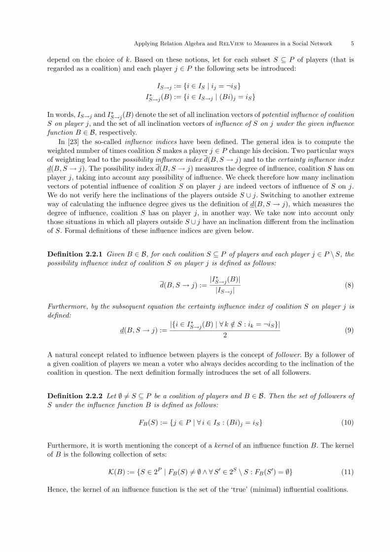
depend on the choice of k. Based on these notions, let for each subset S ⊆ P of players (that isregarded as a coalition) and each player j ∈ P the following sets be introduced:

IS→j := {i ∈ IS | ij = ¬iS}

I∗S→j(B) := {i ∈ IS→j | (Bi)j = iS}

In words, IS→j and I∗S→j(B) denote the set of all inclination vectors of potential influence of coalitionS on player j, and the set of all inclination vectors of influence of S on j under the given influencefunction B ∈ B, respectively.

In [23] the so-called influence indices have been defined. The general idea is to compute theweighted number of times coalition S makes a player j ∈ P change his decision. Two particular waysof weighting lead to the possibility influence index d(B, S → j) and to the certainty influence indexd(B, S → j). The possibility index d(B, S → j) measures the degree of influence, coalition S has onplayer j, taking into account any possibility of influence. We check therefore how many inclinationvectors of potential influence of coalition S on player j are indeed vectors of influence of S on j.We do not verify here the inclinations of the players outside S ∪ j. Switching to another extremeway of calculating the influence degree gives us the definition of d(B, S → j), which measures thedegree of influence, coalition S has on player j, in another way. We take now into account onlythose situations in which all players outside S ∪ j have an inclination different from the inclinationof S. Formal definitions of these influence indices are given below.

Definition 2.2.1 Given B ∈ B, for each coalition S ⊆ P of players and each player j ∈ P \S, thepossibility influence index of coalition S on player j is defined as follows:

d(B, S → j) :=|I∗S→j(B)|

|IS→j |(8)

Furthermore, by the subsequent equation the certainty influence index of coalition S on player j isdefined:

d(B, S → j) :=|{i ∈ I∗S→j(B) | ∀ k /∈ S : ik = ¬iS}|

2(9)

A natural concept related to influence between players is the concept of follower. By a follower ofa given coalition of players we mean a voter who always decides according to the inclination of thecoalition in question. The next definition formally introduces the set of all followers.

Definition 2.2.2 Let ∅ 6= S ⊆ P be a coalition of players and B ∈ B. Then the set of followers ofS under the influence function B is defined as follows:

FB(S) := {j ∈ P | ∀ i ∈ IS : (Bi)j = iS} (10)

Furthermore, it is worth mentioning the concept of a kernel of an influence function B. The kernelof B is the following collection of sets:

K(B) := {S ∈ 2P | FB(S) 6= ∅ ∧ ∀S′ ∈ 2S \ S : FB(S′) = ∅} (11)

Hence, the kernel of an influence function is the set of the ‘true’ (minimal) influential coalitions.


2.3 Majority and influence by trend-setters

In the preceding two subsections we have defined the different indices and notions dealing withcoalitions, influence and followers with respect to an arbitrary influence function B ∈ B and anarbitrary group decision function gd ∈ G. In practice, however, only a very small number of suchfunctions is used.

Group decisions almost always are based on majority. This means that for each inclinationvector i ∈ I and each influence function B ∈ B, the output of gd : B(I) → {0, 1} for the decisionvector Bi as input is 1 if the size of the set {j ∈ P | (Bi)j = 1} is at least [n

2 ]+1, where [x] denotesthe least natural number greater than or equal to x. In the remaining cases, gd(Bi) yields 0 asresult. Instead of this so-called simple majority, in specific cases also other majority rules are used,e.g., 2

3 -majority or even 34 -majority.

Influences in a social network essentially are based on dependency relationships, which ade-quately can be modeled by a dependency graph. The vertices of such a directed loop-free graph arethe players. For different players j, k ∈ P there is an arc from j to k iff j is a so-called trend-setterfor k, that is, the vote of k may be influenced by the inclination of j. Then k is called a depen-dent player. Players without trend-setters (in terms of graph theory: the sources) are said to beindependent.

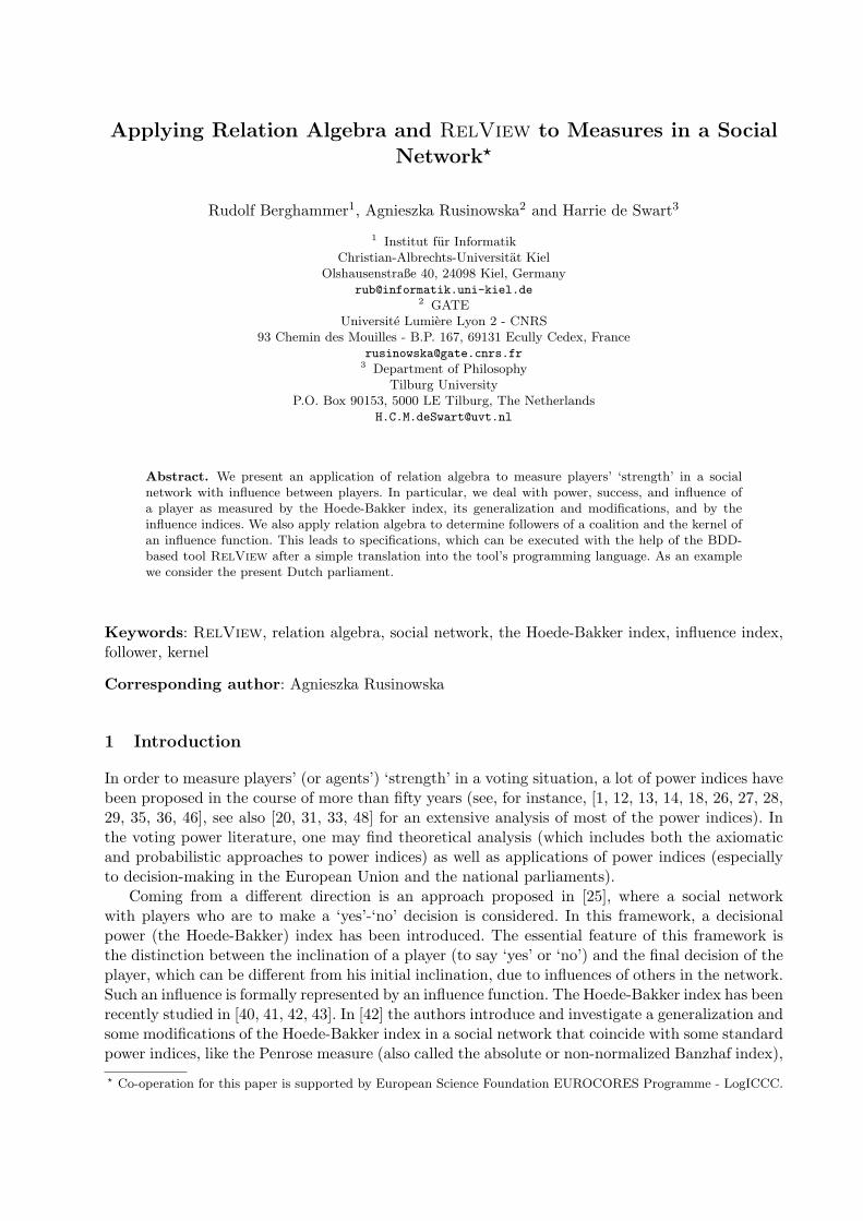
Example 2.3.1. To give a concrete example, the following picture (generated with the help ofRelView) shows the dependency graph of a social network with a set P of six players 1, 2, 3, 4, 5and 6, where the vertex with label ‘k’ corresponds to player k, 1 ≤ k ≤ 6. Since in Sections 3 and4 we will use this social network as running example to illustrate the developed relation-algebraicspecifications, in the dependency graph also a coalition S consisting of the three players 2, 3, 5 isindicated by black vertices.

As one can see from the directed arcs of the graph, the independent players are 1, 5 and 6 (noingoing arcs), and the dependent players are 2, 3 and 4. The vote of player 2 depends on its threetrendsetters (graph-theoretic predecessors) 1, 5 and 6, the vote of player 3 depends on its uniquetrend-setter 2, and the vote of player 4 depends on its two trend-setters 2 and 5.

Now, assume i ∈ I to be an inclination vector and we want to define the decision vector Bi interms of the dependency graph. Of course, for an independent player k ∈ P we are allowed to define(Bi)k := ik, i.e., to presume that he does not change his vote. On the other hand, a dependentplayer k ∈ P will always follow his sole trend-setter j ∈ P if there is exactly one. In this case,hence, we put (Bi)k := ij . It is reasonable to generalize this in such a way that a dependent playeralways follows his trend-setters if they have the same inclination. However, a problem appears ifthere are at least two trend-setters player k ∈ P depends on, and they have different inclinations.Which trend-setter should the dependent player k follow? There are several possibilities to definethe influence function in such a case. Usually two possibilities are considered:

- Following only unanimous trend-setters: Here the vote of player k is equal to the inclination ofhis trend-setters if they all have the same inclination. Otherwise, player k votes according tohis own inclination.


- Following a majority of trend-setters: Here k votes as the inclination of the majority of histrend-setters is. Assuming that player k has t trend-setters, this means that if there are atleast [ t

2 ] + 1 trend-setters of k with the same inclination, k votes according to this inclination.Otherwise, k follows his own inclination.

As in the case of group decisions, also in the second specification of the influence function via trend-setters, simple majority may be replaced by other majority rules. In the remainder of this paper,however, we restrict our analysis to simple majority in the case of the influence rule ‘following amajority of trend-setters’.

3 Relation Algebra and Modeling of Inclination Vectors

In the first part of this section we present the facts on relation algebra that are necessary to dealwith the relation-algebraic specifications and algorithms of the key concepts of Section 2. For moredetails on relations and relation algebra, see e.g., [47] or [11]. Next we model inclination vectorsand sets of inclination vectors within relation algebra. In the last part of this section we brieflydescribe the RelView tool.

3.1 Relational preliminaries

If X and Y are sets, then a subset R of the Cartesian product X × Y is called a (binary) relationwith domain X and range Y . We denote the set (in this context also called type) of all relationswith domain X and range Y by [X ↔Y ] and write R : X ↔Y instead of R ∈ [X ↔Y ]. If Xand Y are finite sets of size m and n respectively, then we may consider a relation R : X ↔Yas a Boolean matrix with m rows and n columns and entries from {0, 1}. The Boolean matrixinterpretation of relations is well suited for many purposes. For instance, it is used as one of thegraphical representations of relations within the RelView tool, and it is in line with the Booleanvector approach of Section 2. Therefore, in this paper we often use Boolean matrix terminologyand notation. In particular, we speak about columns, rows and entries of a relation and write Rx,y

instead of 〈x, y〉 ∈ R or x R y.

We assume the reader to be familiar with the basic operations on relations, viz. RT (transposi-tion, conversion), R (complement, negation), R ∪ S (union, join), R ∩ S (intersection, meet), RS(composition, multiplication), and the special relations O (empty relation), L (universal relation),and I (identity relation). If R is included in S we write R ⊆ S, and equality of R and S is denotedas R = S.

The expression syq(R, S) := RT S ∩ RTS is by definition the symmetric quotient syq(R, S) :

Y ↔Z of two relations R : X ↔Y and S : X ↔Z. Many properties of this construct can be found,for example, in [47]. In the present paper, we will only use that for all y ∈ Y and z ∈ Z therelationship syq(R, S)y,z holds iff for all x ∈ X the equivalence Rx,y ↔ Sx,z is valid, i.e., if they-column of R and the z-column of S coincide.

Given a Cartesian product X × Y of two sets X and Y , there are two projection functionswhich decompose a pair u = (u1, u2) into its first component u1 and its second component u2. Fora relation-algebraic approach it is useful to consider instead of these functions the correspondingprojection relations π : X×Y ↔X and ρ : X×Y ↔Y such that for all pairs u ∈ X × Y andelements x ∈ X and y ∈ Y we have πu,x iff u1 = x and ρu,y iff u2 = y. Projection relations enableus to describe the well-known pairing operation of functional programming relation-algebraically asfollows: For relations R : Z ↔X and S : Z ↔Y we define their pairing (frequently also called fork ortupling) [R, S] : Z ↔X×Y by [R, S] := RπT∩SρT. Then for all z ∈ Z and pairs u = (u1, u2) ∈ X×Ya simple reflection shows that [R, S]z,u iff Rz,u1

and Sz,u2.


3.2 Modeling inclination vectors and sets of inclination vectors

Relation algebra offers some simple and elegant ways to describe subsets of a given set. For modelinginfluence vectors, decision vectors, and sets of followers, we will use column vectors. Following [47],these are relations v (analogously to linear algebra we use lower-case letters to denote vectors) withv = vL. As for a column vector the range is irrelevant, we consider in the following only vectorsv : X ↔1 with a specific singleton set 1 := {⊥} as range. A column vector v : X ↔1 can beconsidered as a Boolean matrix with exactly one column, i.e., as a Boolean column vector, and itdescribes (or: is a description of) the subset {x ∈ X | vx,⊥} of its domain X. A non-empty columnvector v is a column point if vvT ⊆ I, i.e., it is injective in the relational sense. This means that itrepresents a singleton subset of its domain or an element from it, if we identify a singleton set {x}with the element x. In the Boolean matrix model, hence, a column point v : X ↔1 is a Booleancolumn vector in which exactly one entry is 1.

Vectors also allow to formalize the notions of y-columns and x-rows. E.g., for a relation R :X ↔Y and y ∈ Y , the column vector v : X ↔1 equals the y-column of R if for all x ∈ X we havevx,⊥ iff Rx,y.

For modeling kernels and subsets of the sets I and B(I), where the influence function B is givenby one of the rules ‘following only unanimous trend-setters’ and ‘following a majority of trend-setters’ of Subsection 2.3, we will use row vectors. These relations are defined as the transposes ofcolumn vectors. Again we only will need row vectors v of the specific type [1↔Y ] that correspondto Boolean row vectors. Then v describes the subset {y ∈ Y | v⊥,y} of its range Y . The distinctionbetween column vectors and row vectors is not essential. In the context of this paper, however, itis very helpful for the visualization of results of relational computations. This, hopefully, becomesclear by the subsequent continuation of our running example.

Example 3.2.1. In Example 2.3.1 we have introduced a social network with a set P of six players1, 2, 3, 4, 5 and 6. The following picture shows the membership relation1 M : P ↔ 2P between P andits powerset 2P as 6 × 64 Boolean RelView-matrix, where a black square means a 1-entry (i.e.,the relationship holds) and a white square means a 0-entry (i.e., the relationship does not hold).

If we consider inclination vectors as relational column vectors, then this membership relationcolumn-wisely enumerates the set I of all inclination vectors, since its 64 columns exactly cor-respond to the 64 possible inclination vectors of the six players, and these again exactly correspondto the 64 possible subsets of the set of players. For instance, the first column corresponds to theinclination vector where each player has the inclination ‘no’, and the fourth column correspondsto the inclination vector where the players 5 and 6 have the inclination ‘yes’ and the remainingplayers have the inclination ‘no’.

In the same way, we can obtain a 6 × 64 Boolean RelView-matrix showing decisions of theplayers, where the X-column corresponds to the decision vector obtained from the X-column of M

representing the inclination vector. Suppose, for instance, that all players are independent, that is,that we deal with the identity function, Bi = i for each i ∈ I.

The next RelView-picture shows a row vector m : 1↔ 2P with 64 columns that describes asubset of the powerset 2P , i.e., a subset of the set I if we identify X ∈ 2P with the inclinationvector i ∈ I where exactly the players of X vote ‘yes’.

1 A membership relation M : X ↔ 2X relates x ∈ X and Y ∈ 2X iff x ∈ Y . It should be emphasized that binarydecision diagrams allow a very efficient implementation of M that uses in the worst case 3|X| + 1 BDD-verticesonly. This implementation is part of RelView; see [5].


This row vector describes the set of the inclination vectors where the majority of the players votes‘yes’. This becomes clear if we compare the columns of both RelView-pictures. Doing so, we obtainthat for all X ∈ 2P the relationship m⊥,X holds iff the number of 1-entries in the X-column of M

is strictly larger than the number of 0-entries in the X-column of M.

Besides column vectors, row vectors and membership relations, injective (embedding) mappingsare another way of modeling sets. Given a relation ı : Z ↔X, that is, an injective mapping inthe relational sense of [47], Z may be regarded as a subset of X by identifying it with its imageunder ı. Then the column vector ıTL : X ↔1 describes Z in the above sense. By removing all pairs(x, x) with x /∈ Z from the identity relation I : X ↔X, the transition in the other direction is alsopossible, that is, the construction of a relation inj (v) : Z ↔X from a given column vector v : X ↔1

describing Z in such a way that inj (v)z.x holds iff z = x for all z ∈ Z and x ∈ X. Such a relationis called the injective embedding generated by v and is also used in our applications. Namely, ifthe row vector v : 1↔ 2P describes a subset S of 2P in the sense above, and M : P ↔ 2P is the

membership relation, then for all x ∈ X and Y ∈ S we get the equivalence of (M inj (vT)T)x,Y and

x ∈ Y . This means that the elements of S are described precisely by the columns of the relation

M inj (vT)T

: X ↔S.

3.3 The Kiel RelView tool

Relation algebra has a fixed and surprisingly small set of constants and operations which (in thecase of finite carrier sets) can be implemented very efficiently. Since 1993, at Kiel University we havedeveloped a computer system for the visualization and manipulation of relations and for relationalprototyping and programming, called RelView. The tool is written in the C programming languageand makes full use of the X-windows graphical user interface. Details and applications can be found,for instance, in [4, 2, 9].

RelView is an interactive and graphic-oriented tool. In it all data are represented as rela-tions which the system visualizes in two different ways. First, for relations, for which domain andrange coincide, it offers a representation as directed graphs as already shown in Example 2.3.1.This includes sophisticated algorithms for drawing graphs nicely. Alternatively, as already shownin Example 3.2.1, arbitrary relations may be depicted as Boolean matrices (with, if desired, rowand column labels for explanatory purposes). This second representation is very useful for visuallyediting and also for discovering various structural properties that are not evident from a represen-tation of relations as directed graphs. Because RelView computations frequently use very largerelations, for instance, membership relations, the system uses a very efficient implementation ofrelations via reduced ordered binary decision diagrams. See [5] for its description.

The RelView tool can manage as many relations simultaneously as memory allows and theuser can manipulate and analyse them by pre-defined operations, tests and user-defined relationalfunctions and relational programs. The pre-defined operations on relations include, for instance, ^,-, &, |, and * for transposition, complement, intersection, union, and composition; the relationaltests include, for instance, incl, eq, and empty for testing inclusion, equality, and emptiness ofrelations. All that can be accessed through a lot of command buttons and simple mouse-clicks. Butthe usual way is to use the pre-defined operations and tests to construct relational functions andrelational programs and next to evaluate the relation-algebraic expressions that are built from therelations of RelView’s workspace using the tool’s programming language.

Relational functions are defined as it is customary in mathematics, i.e., by a function name, alist of parameters and a relation-algebraic expression. A relational program is much like a function


procedure in the programming languages Pascal or Modula 2, except that it only uses relations asdata type. It starts with a head line containing the program name and the formal parameters. Thenthe declaration of the local relational domains, functions, and variables follows. Domain declarationscan be used to introduce projection relations and pairings of relations in the case of Cartesianproducts, and injection relations and sums of relations in the case of disjoint unions, respectively.The third part of a program is the body, a while-program over relations. As a program computes avalue, finally, its last part consists of a return-clause, which is a relation-algebraic expression whosevalue after the execution of the body is the result. The following example of a RelView-programClasses (formally developed in [3]) computes for an equivalence relation R : X ↔X with a set Cof equivalence classes the canonical epimorphism from X to C as a relation Φ : X ↔C.

Classes(R)

DECL Phi, v, p

BEG Phi = R*point(Ln1(R));

v = -Phi;

WHILE -empty(v) DO

p = point(v);

Phi = (Phi^ + (R*p)^)^;

v = v & -(R*p) OD

RETURN Phi

END.

Since Φ is the relational version of the canonical epimorphism, we have for all x ∈ X and C ∈ Cthat Φx,C iff x belongs to C. Hence, if we consider the columns of the result of the RelView-program Classes as single vectors, then these vectors are pair-wise disjoint and precisely describethe elements of the set C in the sense explained above.

4 Relation-algebraic Description of Measures in a Social Network

In this section we show how the concepts introduced in Section 2 can be transformed into relation-algebraic specifications that immediately lead to RelView-code. This allows to compute powerindices, influence indices, sets of followers and kernels by means of the tool. We demonstrate thisby depicting some of the RelView-matrices and -vectors that we have obtained for our runningexample.

4.1 Computing decision vectors and group decisions

We assume a social network with a set P of players. Let D : P ↔P be the relation of the dependencygraph of the network. The latter property means that there is an arc from a player j ∈ P to aplayer k ∈ P iff Dj,k holds. Then the set of the dependent players relation-algebraically is describedby the column vector

depend(D) := DTL (12)

of type [P ↔1], where the used L has type [P ↔1], too.In Subsection 3.2 we have shown that the set I of all inclination vectors immediately can be

modeled by the columns of the membership relation M : P ↔ 2P . Due to this fact, in the remainderof this section we regard inclination vectors and the corresponding decision vectors as relationalcolumn vectors i : P ↔1 and Bi : P ↔1, respectively. Our first goal is to develop a column-wiseenumeration of the set B(I) of decision vectors with relation-algebraic means, where the influencefunction B is given by the rule ‘following only unambiguous trend-setters’. As a preparatory step,we treat the transformation from i to Bi for a single inclination vector i within relation algebra.


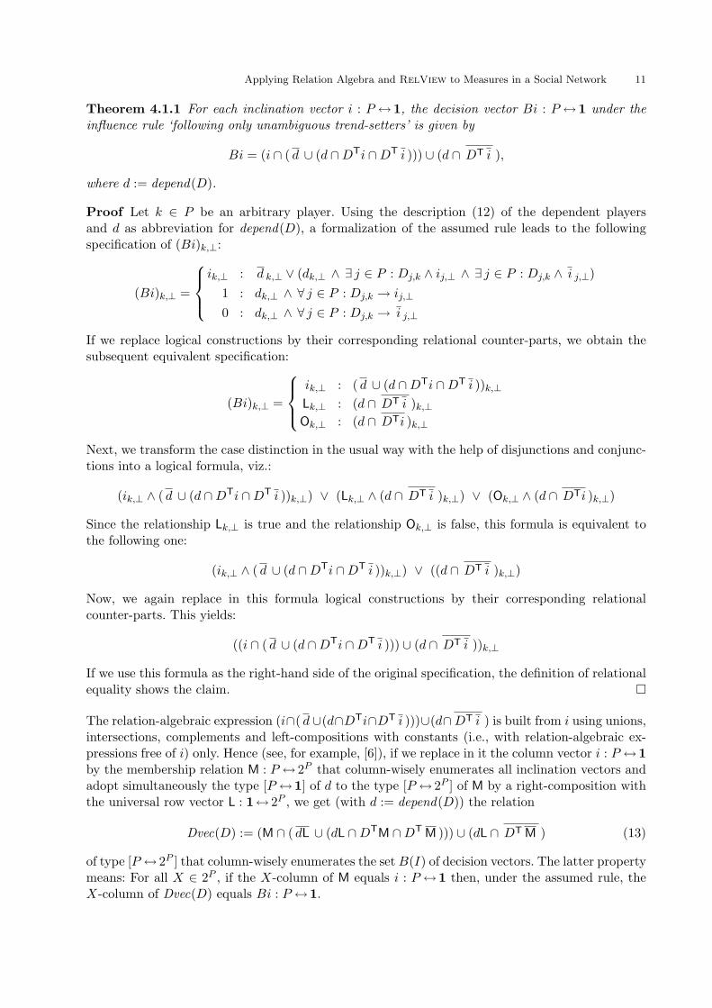
Theorem 4.1.1 For each inclination vector i : P ↔1, the decision vector Bi : P ↔1 under theinfluence rule ‘following only unambiguous trend-setters’ is given by

Bi = (i ∩ ( d ∪ (d ∩ DTi ∩ DT i ))) ∪ (d ∩ DT i ),

where d := depend(D).

Proof Let k ∈ P be an arbitrary player. Using the description (12) of the dependent playersand d as abbreviation for depend(D), a formalization of the assumed rule leads to the followingspecification of (Bi)k,⊥:

(Bi)k,⊥ =

ik,⊥ : d k,⊥ ∨ (dk,⊥ ∧ ∃ j ∈ P : Dj,k ∧ ij,⊥ ∧ ∃ j ∈ P : Dj,k ∧ i j,⊥)

1 : dk,⊥ ∧ ∀ j ∈ P : Dj,k → ij,⊥

0 : dk,⊥ ∧ ∀ j ∈ P : Dj,k → i j,⊥

If we replace logical constructions by their corresponding relational counter-parts, we obtain thesubsequent equivalent specification:

(Bi)k,⊥ =

ik,⊥ : ( d ∪ (d ∩ DTi ∩ DT i ))k,⊥

Lk,⊥ : (d ∩ DT i )k,⊥

Ok,⊥ : (d ∩ DTi )k,⊥

Next, we transform the case distinction in the usual way with the help of disjunctions and conjunc-tions into a logical formula, viz.:

(ik,⊥ ∧ ( d ∪ (d ∩ DTi ∩ DT i ))k,⊥) ∨ (Lk,⊥ ∧ (d ∩ DT i )k,⊥) ∨ (Ok,⊥ ∧ (d ∩ DTi )k,⊥)

Since the relationship Lk,⊥ is true and the relationship Ok,⊥ is false, this formula is equivalent tothe following one:

(ik,⊥ ∧ ( d ∪ (d ∩ DTi ∩ DT i ))k,⊥) ∨ ((d ∩ DT i )k,⊥)

Now, we again replace in this formula logical constructions by their corresponding relationalcounter-parts. This yields:

((i ∩ ( d ∪ (d ∩ DTi ∩ DT i ))) ∪ (d ∩ DT i ))k,⊥

If we use this formula as the right-hand side of the original specification, the definition of relationalequality shows the claim. �

The relation-algebraic expression (i∩( d ∪(d∩DTi∩DT i )))∪(d∩ DT i ) is built from i using unions,intersections, complements and left-compositions with constants (i.e., with relation-algebraic ex-pressions free of i) only. Hence (see, for example, [6]), if we replace in it the column vector i : P ↔1

by the membership relation M : P ↔ 2P that column-wisely enumerates all inclination vectors andadopt simultaneously the type [P ↔1] of d to the type [P ↔ 2P ] of M by a right-composition withthe universal row vector L : 1↔ 2P , we get (with d := depend(D)) the relation

Dvec(D) := (M ∩ ( dL ∪ (dL ∩ DTM ∩ DT

M ))) ∪ (dL ∩ DT M ) (13)

of type [P ↔ 2P ] that column-wisely enumerates the set B(I) of decision vectors. The latter propertymeans: For all X ∈ 2P , if the X-column of M equals i : P ↔1 then, under the assumed rule, theX-column of Dvec(D) equals Bi : P ↔1.


Having obtained a relation-algebraic specification for the column-wise enumeration of the de-cision vectors, our next goal is to obtain with the help of (13) a relation-algebraic specification ofthe group decisions under majority as decision rule via a row vector. To reach the goal, we assumethat a row vector m : 1↔ 2P is available such that for all X ∈ 2P we have m⊥,X iff |X| ≥ [ |P |

2 ] + 1.In RelView such a vector can be easily obtained with the help of the base operation cardfilter2 as

m := cardfilter(L, w)T

, (14)

where the first argument L : 2P ↔1 describes the entire powerset 2P , and the second argumentw : W ↔1 determines the threshold for majority by its length, i.e., fulfils |W | = [ |P |

2 ] + 1. Basedon (14), we can specify the desired row vector as shown now.

Theorem 4.1.2 Let, based on the specifications (13) and (14), the row vector gdv(D) of type[1↔ 2P ] be defined by

gdv(D) := m syq(M,Dvec(D)),

where M : P ↔ 2P is the membership relation. Then we have for all X ∈ 2P : If the decision vectorBi : P ↔1 equals the X-column of Dvec(D), then gdv(D)⊥,X holds iff the number of 1-entries in

Bi is at least [ |P |2 ] + 1.

Proof We calculate as given below, where the assumption that the X-column of Dvec(D) equalsBi is used in the last step, and the inclination vector i(Y ) introduced in this step coincides withthe Y -column of M.

gdv(D)⊥,X ⇐⇒ (m syq(M,Dvec(D)))⊥,X

⇐⇒ ∃Y ∈ 2P : m⊥,Y ∧ syq(M,Dvec(D))Y,X

⇐⇒ ∃Y ∈ 2P : m⊥,Y ∧ (∀ k ∈ P : Mk,Y ↔ Dvec(D)k,X)

⇐⇒ ∃Y ∈ 2P : |Y | ≥ [ |P |2 ] + 1 ∧ (∀ k ∈ P : Mk,Y ↔ Dvec(D)k,X)

⇐⇒ ∃Y ∈ 2P : |Y | ≥ [ |P |2 ] + 1 ∧ i(Y ) = Bi

Now the claim follows from the simple fact that the number of 1-entries in the column vector i(Y )

equals |Y |. �

Summing up, we have for the influence function B defined by the rule ‘following only unambiguoustrend-setters’ and for the group decision function gd defined by simple majority: If the inclinationvector i : P ↔1 is given by the X-column of the membership relation M : P ↔ 2P , then thecorresponding decision vector Bi : P ↔1 is given by the X-column of the relation Dvec(D) : P ↔ 2P

and, furthermore, gd(Bi) = 1 iff gdv(D)⊥,X holds.

Example 4.1.1. We have transformed the above relation-algebraic specifications into RelView-code. To give examples how such programs look like, we present in the following the code for bothspecifications. In the following RelView-programs Dvec and gdv the calls epsi(O(D)) of the pre-defined operation epsi compute the membership relation M : P ↔ 2P , and the calls L1n(M) of the

2 If v : 2M ↔1 represents the subset S of 2M and the size of the domain of w : W ↔1 is at most |M |+1, then for allX ∈ 2M we have cardfilter(v, w)X,⊥ iff X ∈ S and |X| < |W |. Hence, the complement of cardfilter(L, w) representsthe subset of 2M whose elements have at least size |W |.


pre-defined operation L1n yield the row vector L : 1↔ 2P .3

Dvec(D)

DECL M, d

BEG M = epsi(O(D));

d = D^*L1n(M)

RETURN (M & (-d | (d & D^*M & D^*-M))) | (d & -(D^*-M))

END.

gdv(D,w)

DECL M, m

BEG M = epsi(O(D));

m = -cardfilter(L1n(M)^,w)^

RETURN m*syq(M,Dvec(D))

END.

Applied to the relation D of our running example and a column vector w of length 4 (thethreshold of majority) in the case of the second program, we obtained by their means the followingresults for Dvec(D) and gdv(D). The 64 columns of the 6 × 64 RelView-matrix represent the 64decision vectors obtained from the 64 inclination vectors, and the entries of the 1 × 64 row vectorbelow this matrix indicate the group decision for each decision vector.

Let us explain these results by the specific inclination vectors treated in Example 3.2.1. For the firstcolumn of the membership relation M of Example 3.2.1, where each player votes ‘no’, we obtain ‘no’also as decision of each player as well as of the entire group. The same is the case if the inclinationof the players 5 and 6 is ‘yes’ and that of the remaining players is ‘no’; cf. the fourth columns ofM, Dvec(D) and gdv(D).

We also have developed a RelView-program that computes the column-wise enumeration of thedecision vectors under ‘following a majority of the trend-setters’ as the influence rule by handlingone after another the columns of the membership relation via a loop. If we use this program inthe case of our running example, we obtain the following RelView-matrix and row vector for thedecision vectors and the group decisions, respectively.

In contrast with the influence rule ‘following only unambiguous trend-setters’, now the inclinations‘yes’ of the players 5 and 6 and ‘no’ of the remaining players yield a decision, where player 2 changes

3 We need n and 1 in the pre-defined RelView-operations for typing. If R : X ↔Y is a relation, then L(R) yields theuniversal relation L of type [X ↔Y ], Ln1(R) yields the universal column vector L of type [X ↔1], and L1n(R) yieldsthe universal row vector L of type [1↔Y ]. Hence, in the RelView-programs L1n(M) is the universal row vectorof type [1↔ 2P ] and so its transposition the universal column vector of type [2P ↔1]. The RelView-operationcardfilter works on column-vectors; that is the only reason for the transposition here.


his opinion from ‘no’ to ‘yes’, because of the ‘yes’-vote of the majority of the trend-setters player 2depends on. In spite of this change, the group’s decision remains ‘no’.

An example where the different influence rules yield different group decisions for the sameinclination vector is given by the 8th columns of the matrices and row vectors, respectively. If theinclination of the players 4, 5 and 6 is ‘yes’ and that of the remaining players is ‘no’, then ‘followingonly unambiguous trend-setters’ implies ‘inclination equals decision’ and the group decision ‘no’.Nevertheless, ‘following a majority of the trend-setters’ implies that also player 2 finally votes ‘yes’,so that the collective vote becomes ‘yes’, too.

As we can see from the matrices of this example, within the column-wise enumeration of thedecision vectors E := Dvec(D) some columns may occur several times. But it is very easy to obtaina representation without multiple columns. We only have to compute the canonical epimorphism Φof the equivalence relation syq(E, E) via the relational program Classes of Subsection 3.3. ThenEΦ yields the desired result.

4.2 Computing power indices

Now, we demonstrate how to compute the indices presented in Subsection 2.1 with relation-algebraicmeans. The main steps are to determine four row vectors of type [1↔ 2P ] which describe the foursets I++

k , I+−k , I−+

k and I−−k , respectively. Since RelView yields for each computed relation also the

number of its 1-entries (i.e., its set-theoretic size), from the vector descriptions we get the numbers|I++

k |, |I+−k |, |I−+

k | and |I−−k |, and from these also the various power indices using straightforwardly

their specifications of Subsection 2.1. Note, that the set I+ used in the definition of the indicesM1GHBk, M4GHBk and MGHB is already described by the row vector gdv(D) of Theorem 4.1.2or its analogon in the case of the rule ‘following a majority of the trend-setters’.

We assume that the player k ∈ P , on which the four sets I++k , I+−

k , I−+k and I−−

k depend,is described by a column point p : P ↔1 in the relational sense. As the definitions of the setsalso use the values gd(Bi) for i ∈ I, we assume, furthermore, that the group decision row vectorg := gdv(D) is at hand (where the influence rule used for its computation is arbitrary). Then weare able to prove the following result.

Theorem 4.2.1 Let, depending on the column point p : P ↔1 and the row vector g : 1↔ 2P , thefour vectors ipp(p, g), ipm(p, g), imp(p, g) and imm(p, g) of type [1↔ 2P ] be defined as follows,where M : P ↔ 2P is the membership relation:

ipp(p, g) := pTM ∩ g ipm(p, g) := pTM ∩ g

imp(p, g) := pT M ∩ g imm(p, g) := pT M ∩ g

Then we have for all X ∈ 2P : If the X-column of M equals the inclination vector i : P ↔1, thenwe have that ipp(p, g)⊥,X holds iff i ∈ I++

k , ipm(p, g)⊥,X holds iff i ∈ I+−k , imp(p, g)⊥,X holds iff

i ∈ I−+k , and imm(p, g)⊥,X holds iff i ∈ I−−

k .

Proof The first claim follows from

ipp(p, g)⊥,X ⇐⇒ (pTM ∩ g)⊥,X

⇐⇒ ∃ j ∈ P : pj,⊥ ∧ Mj,X ∧ g⊥,X

⇐⇒ ∃ j ∈ P : j = k ∧ Mj,X ∧ g⊥,X p describes k

⇐⇒ Mk,X ∧ g⊥,X gd(Bi) = 1 iff gdv(D)⊥,X

⇐⇒ ik,⊥ ∧ gd(Bi) = 1 assumption

⇐⇒ i ∈ I++k


since the relationship ik,⊥ is nothing else than ik = 1 for the k-component of a Boolean vector inthe sense of Section 2. In the same way the remaining equivalences can be calculated. �

Due to this theorem, the row vector ipp(p, g) precisely designates those columns of the membershiprelation M which belong to the set I++

k , and the remaining three row vectors of the theorem dothe same for the three sets I+−

k , I−+k and I−−

k , respectively. Once more it is very easy to translatethe relation-algebraic specifications of Theorem 4.2.1 into the programming language of RelView.Subsequently, we show some results for our running example. We restrict our analysis to the Hoede-Bakker index defined in (1).

Example 4.2.1. In the following, we concentrate on player 2 which is influenced by the threetrend-setters 1, 5 and 6. Using ‘following only unambiguous trend-setters’ as influence rule, thefirst row of the following 2 × 64 RelView-matrix depicts the row vector ipp(p, g), i.e., preciselydesignates those columns of the membership relation M : P ↔ 2P that belong to the set I++

2 . Thesecond row of the matrix does the same for I+−

2 .

Counting the 1-entries of the single rows, we obtain that in 24 cases the inclination ‘yes’ of player2 coincides with the group decision ‘yes’, and in 8 cases the inclination ‘yes’ of player 2 is opposedto the group decision ‘no’. Hence, in the social network of the example, the Hoede-Bakker indexfor player 2 is 1

32(24 − 8) = 0.5.The next picture shows, again by means of one matrix, the RelView-representations of the two

sets I++2 (first row) and I+−

2 (second row) of the inclination vectors with ‘following the majority ofthe trend-setters’ as the influence rule.

Counting the 1-entries of the single rows, we obtain here that in 16 cases player 2’s inclination andthe group vote are ‘yes’, and in the same number of cases player 2 has the inclination ‘yes’, butthe group says ‘no’. Under this rule, hence, we have 1

32(16− 16) = 0 as the Hoede-Bakker index forplayer 2.

We have also computed the Hoede-Bakker indices for the other players. In the case of the influencerule ‘following only unambiguous trend-setters’, we have obtained that not an independent player,but player 2 is the most powerful player of the network in our running example. For the independentplayers we have obtained (in the case of both rules) the Hoede-Bakker indices 0.125 (players 1and 6) and 0.25 (player 5). This result agrees with observations that frequently can be made inpractice, e.g., if the network is given by a hierarchic administration structure. If players may obtaininstructions from more than one ‘superior’ player, then not the independent players (the big bosses)are the most powerful ones, but those in the middle of the hierarchy.

4.3 Computing influence indices, followers and kernels

In the following, we assume a coalition S of players to be described by a column vector s : P ↔1,and a single player j ∈ P to be described by a column point p : P ↔1. We want to compute thepossibility influence index of S on player j. Since it is defined by means of the sizes of the sets IS→j

and I∗S→j(B), our task is to describe these sets within relation algebra. A translation of the resultsinto RelView-code then allows to proceed exactly as in the case of the power indices.

Both, IS→j and I∗S→j(B) are subsets of IS . Therefore, as a preparatory step we describe thelatter set of inclination vectors with relation-algebraic means. Doing so, projection relations andthe pairing operation come into the play.


Theorem 4.3.1 Assume s : P ↔1 as description of the coalition S ⊆ P and the row vector is(s)of type [1↔ 2P ] to be defined as

is(s) := [sT, sT] (πM ∪ ρM) ∩ ( ρM ∪ πM) ,

where M : P ↔ 2P is the membership relation, and π : P×P ↔P and ρ : P×P ↔P are theprojection relations in the sense of Subsection 3.1. Then we have for all X ∈ 2P : If the X-columnof M equals the inclination vector i : P ↔1, then is(s)⊥,X holds iff i ∈ IS.

Proof Since the X-column of M equals i, we have for all pairs u = (u1, u2) ∈ P×P the followingequivalence:

iu1,⊥ = iu2,⊥ ⇐⇒ Mu1,X ↔ Mu2,X

⇐⇒ (πM)u,X ↔ (ρM)u,X

⇐⇒ ((πM)u,X → (ρM)u,X) ∧ ((ρM)u,X → (πM)u,X)

⇐⇒ (πM u,X ∨ (ρM)u,X) ∧ ( ρM u,X ∨ (πM)u,X)

⇐⇒ ((πM ∪ ρM) ∩ ( ρM ∪ πM))u,X

From this result and since s describes S, we obtain

is(s)⊥,X ⇐⇒ ([sT, sT] (πM ∪ ρM) ∩ ( ρM ∪ πM) )⊥,X

⇐⇒ ∃u ∈ P×P : [sT, sT]⊥,u ∧ (πM ∪ ρM) ∩ ( ρM ∪ πM) u,X

⇐⇒ ∀u ∈ P×P : [sT, sT]⊥,u → ((πM ∪ ρM) ∩ ( ρM ∪ πM))u,X

⇐⇒ ∀u ∈ P×P : su1,⊥ ∧ su2,⊥ → (iu1,⊥ = iu2,⊥)

⇐⇒ ∀u ∈ P×P : u1 ∈ S ∧ u2 ∈ S → (iu1,⊥ = iu2,⊥)

The latter formula of this calculation exactly says that i ∈ IS . �

Hence, the row vector is(s) precisely designates those columns of the membership relation M whichbelong to the set IS . Next, we attack the relation-algebraic specification of the set IS→j , wherej ∈ P is described by the column point p : P ↔1. In the following theorem we relation-algebraicallyspecify a row vector that precisely designates those columns of M which are inclination vectors ofpotential influence of S on j.

Theorem 4.3.2 Assume s : P ↔1 to describe the coalition S ⊆ P , the column point p : P ↔1

to describe the player j ∈ P , the column point q ⊆ s to describe some player k ∈ S, and the rowvector potinf (s, p) of type [1↔ 2P ] to be defined as

potinf (s, p) := ((r ∪ r′) ∩ r ∩ r′ ) inj (is(s)T),

where r := pTM inj (is(s)T)T

and r′ := qTM inj (is(s)T)T

with M : P ↔ 2P as membership relation.Then we have for all X ∈ 2P : If the X-column of M equals the inclination vector i : P ↔1, thenpotinf (s, p)⊥,X holds iff i ∈ IS→j.

Proof From Theorem 4.3.1 we know that the row vector is(s) describes the subset S of 2P thatconsists of those sets Y ∈ 2P for which the Y -column of M is, considered as inclination vector,a member of IS . Furthermore, inj (is(s)T) : S ↔ 2P is the relational description of the identity


mapping from S to 2P ; see Subsection 3.2. Using these facts and the assumption that the X-column of M equals i, we get

potinf (s, p)⊥,X ⇐⇒ (((r ∪ r′) ∩ r ∩ r′ ) inj (is(s)T))⊥,X

⇐⇒ ∃Y ∈ S : ((r ∪ r′) ∩ r ∩ r′ )⊥,Y ∧ inj (is(s)T)Y,X

⇐⇒ ∃Y ∈ S : ((r ∪ r′) ∩ r ∩ r′ )⊥,Y ∧ Y = X

⇐⇒ X ∈ S ∧ ((r ∪ r′) ∩ r ∩ r′ )⊥,X

⇐⇒ i ∈ IS ∧ ((r ∪ r′) ∩ r ∩ r′ )⊥,X

Next, we apply that the column point p describes the player j ∈ P , again we apply the assumptionand get in the case X ∈ S the equivalence

r⊥,X ⇐⇒ ∃ l ∈ P : pl,⊥ ∧ Ml,X ⇐⇒ ∃ l ∈ P : j = l ∧ l ∈ X ⇐⇒ j ∈ X ⇐⇒ ij,⊥.

In the same way4 from the description of k ∈ P by the column vector q and the assumption weobtain that r′⊥,X is equivalent to ik,⊥, i.e., to the k-entry of i to be 1. The latter fact impliesthe equivalence of r′⊥,X and iS = 1 for the Boolean value iS used in the specification of IS→j . Aconsequence of the just shown properties is

((r ∪ r′) ∩ r ∩ r′ )⊥,X ⇐⇒ (r⊥,X ∨ r′⊥,X) ∧ ¬(r⊥,X ∧ r′⊥,X)

⇐⇒ (ij,⊥ ∨ iS = 1) ∧ ¬(ij,⊥ ∧ iS = 1)

⇐⇒ (ij,⊥ ↔ ¬(iS = 1))

⇐⇒ (ij = ¬iS)

since again the relationship ij,⊥ is nothing else than the validity of ij = 1 in the sense of Section 2.Now, a combination of this fact with the result of the above calculation yields

potinf (s, p)⊥,X ⇐⇒ i ∈ IS ∧ (ij = ¬iS)

and this, finally, shows the claim. �

To obtain a row vector inf (s, p, D) of type [1↔ 2P ] that precisely designates those columns of themembership relation M : P ↔ 2P which are inclination vectors of influence of S on j, i.e., membersof I∗S→j(B), we use the equation

I∗S→j(B) = IS→j ∩ {i ∈ IS | (Bi)j = iS}.

The definition of the set {i ∈ IS | (Bi)j = iS} is rather similar to that of the set IS→j ; cf. Subsection2.2. Compared with the latter one, only the expressions Bi and iS are used instead of i and ¬iS .This immediately leads to the relation-algebraic specification of the set I∗S→j(B) by the row vector

inf (s, p, D) := potinf (s, p) ∩ (r ∪ r′) ∩ r ∩ r′ inj (is(s)T) (15)

with now r and r′ given by r := pTDvec(D) inj (is(s)T)T

and r′ := qTM inj (is(s)T)T

(see Theorem4.3.2). This is due to the fact that the decision vectors column-wisely are enumerated via therelation Dvec(D) : P ↔ 2P (where the concrete influence rule is irrelevant) and, for the inclinationvector i : P ↔1 being the X-column of the membership relation M : P ↔ 2P , the relationship((r ∪ r′) ∩ r ∩ r′ )⊥,X does not hold iff ij,⊥ and iS = 1 are equivalent.

In the following, we demonstrate by means of our running example how results of the Rel-

View-programs look like that immediately are obtained from the just developed relation-algebraicspecifications by writing them in the programming language of the tool.

4 In terms of matrices, r equals the j-row of M inj (is(s)T)T

and r′ the k-row of the same relation.


Example 4.3.1. Let us consider the coalition S with players 2, 3 and 5, that is in the depen-dency graph of Example 2.3.1 indicated by black vertices. For this coalition, the set IS contains16 inclination vectors. This follows from the following two RelView-pictures. The first one showsagain the membership relation M : P ↔ 2P of Example 3.2.1 and the second one the row vectoris(s) : 1↔ 2P , where the column vector s : P ↔1 describes S.

The row vector precisely designates those columns of the matrix where the entries 2, 3 and 5 havethe same colour.

Below we show the RelView-representations of the sets IS→j and I∗S→j(B) for those players jwhich are not contained in the coalition S. The first row of the following 2 × 64 RelView-matrixindicates the columns of the membership relation M which are inclination vectors from set IS→1,and the second row indicates the inclination vectors that belong to I∗S→1(B), where ‘following onlyunambiguous trend-setters’ is the influence rule. The next two RelView-matrices do the same forthe sets IS→4 and I∗S→4(B) and the sets IS→6 and I∗S→6(B), respectively. From the three pictureswe obtain that, under the assumed rule, the possibility influence indices of S on the players 1 and6 are 0, and the possibility influence index of S on the player 4 is 1.

The next three RelView-matrices are analogous to the just presented ones, however, with ‘follow-ing the majority of the trend-setters’ as influence rule for the computation of the decision vectors.

Comparing these matrices with the above ones, we get that in the case of our running exampleboth influence rules lead to the same sets and, hence, the same indices.5 In words, the results say:Whatever of the two influence rules is applied, the coalition S is without any influence on theplayers 1 and 6 and in the case of player 4 there is a possibility of influence of S on 4 and it is evenmaximal.

From I∗S→1(B) = I∗S→6(B) = ∅ in the case of both influence rules we immediately get thatthe certainty influence index of S on player 1 as well as on player 6 is 0. The next RelView-picture shows the column-wise enumeration of the set I∗S→4(B) (which is equal under both rules)as computed by the tool. To enhance readability, the used column labels correspond to the columnlabels of the above membership relation.

5 It should be mentioned that the equal results for player k := 4 in our running example are caused by the fact thatit has exactly two trend-setters. In such a case the value (Bi)k computed from i via ‘following only unambiguoustrend-setters’ is the same as that computed via ‘following the majority of the trend-setters’. To give an examplewhere both rules lead to different results, we want to mention that, for S′ := {3, 5} and player 2, we get |IS′→2| = 16and |I∗

S′→2(B)| = 4 if B is given by ‘following only unambiguous trend-setters’, respectively |I∗

S′→2(B)| = 12 if B

is given by ‘following the majority of the trend-setters’.


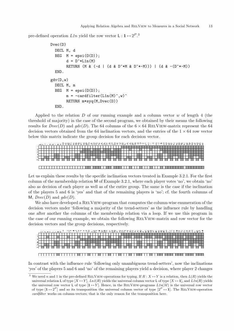
Under both rules for S and player 4 exactly 2 of the eight inclination vectors i ∈ I∗S→4(B) fulfil theproperty ik = ¬iS for all players k not from S. The first one is labeled with 27 (here iS = 1 andik = 0 for k = 1, 4, 6), and the second one is labeled with 38 (and is the complement of the firstone). Hence, the certainty influence index d(B, {2, 3, 5} → 4) is 1.

The relation-algebraic treatment of the certainty influence index is rather similar to that of thepossibility influence index. However, we do not want to go into more details here, and we switchdirectly to followers.

The next theorem shows how sets of followers can be described relation-algebraically by means ofcolumn vectors in the sense of Subsection 3.2. In it, the relations R and Q column-wisely enumeratethe sets IS and B(IS), respectively, and the column point q again is used for specifying for i ∈ IS thespecific Boolean value iS . Once more it is arbitrarily which influence rule is used for the definitionof the influence function B.

Theorem 4.3.3 Assume s : P ↔1 to describe the coalition S ⊆ P , and the column point q ⊆ s todescribe some player k ∈ S. Furthermore, let M : P ↔ 2P be the membership relation. If the columnvector follow(D, s) of type [P ↔1] is defined as

follow(D, s) := syq(QT, RTq)

with relations R := M inj (is(s)T)T

and Q := Dvec(D) inj (is(s)T)T

, then for all j ∈ P we havefollow(D, s)j,⊥ iff j ∈ FB(S).

Proof As in the proof of Theorem 4.3.2, we denote the subset of 2P that is described by the rowvector is(s) : 1↔ 2P with S. Then both R and Q have the type [P ↔S]. Furthermore, we are ableto calculate as given below:

follow(D, s)j,⊥ ⇐⇒ syq(QT, RTq)j,⊥

⇐⇒ ∀X ∈ S : QT

X,j ↔ (RTq)X,⊥

⇐⇒ ∀X ∈ S : Qj,X ↔ (qTR)⊥,X

⇐⇒ ∀ i ∈ IS : (Bi)j,⊥ ↔ iS = 1⇐⇒ j ∈ FS(B)

The fourth step of this calculation uses that there is a one-to-one corrrespondence between the sets2P and I, that X ∈ 2P belongs to S iff the corresponding inclination vector i ∈ I belongs to IS ,that Dvec(D) column-wisely enumerates the decision vectors Bi and that (qTR)⊥,X iff iS = 1 (seethe proof of Theorem 4.3.2). �

Let us again demonstrate what the RelView-program obtained from this theorem yields in thecase of our running example with the coalition S consisting of the players 2, 3 and 5.

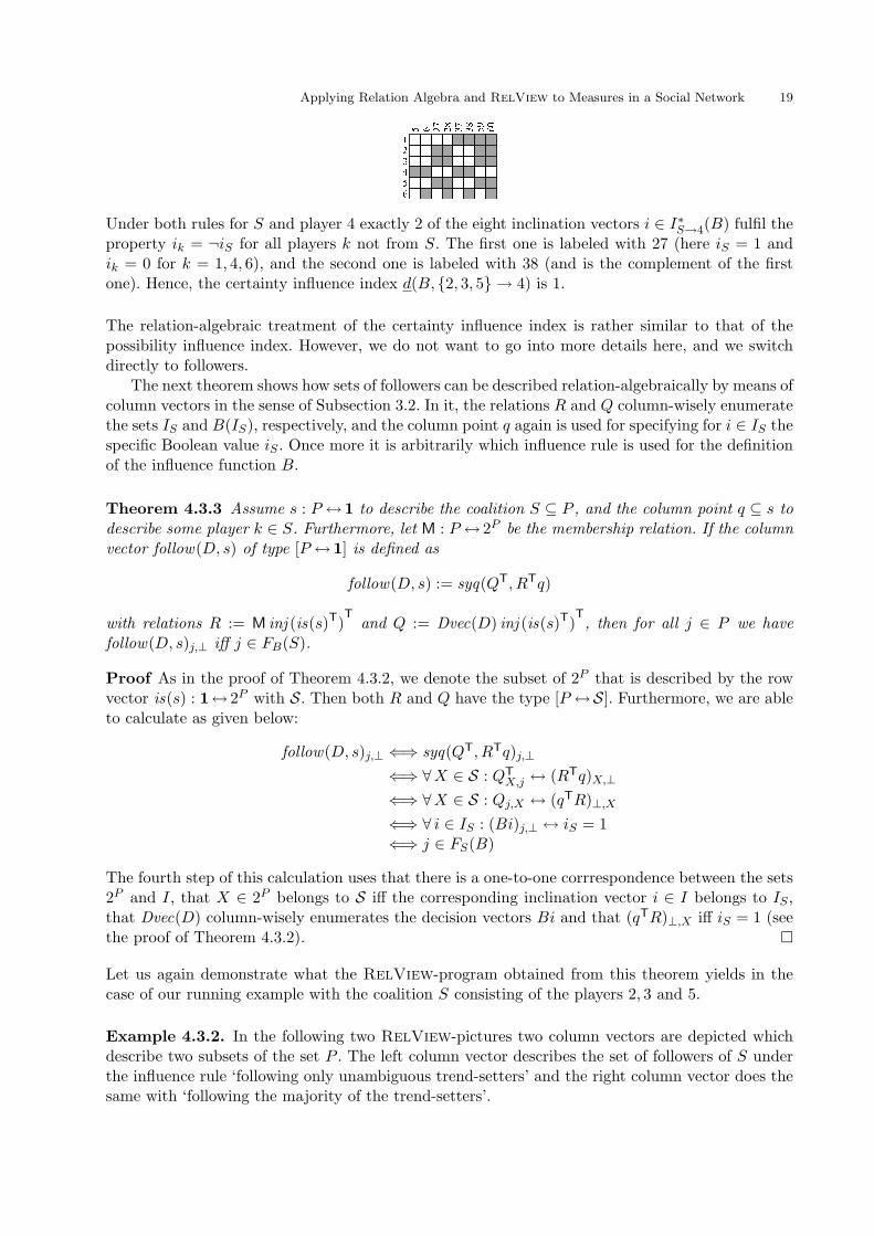
Example 4.3.2. In the following two RelView-pictures two column vectors are depicted whichdescribe two subsets of the set P . The left column vector describes the set of followers of S underthe influence rule ‘following only unambiguous trend-setters’ and the right column vector does thesame with ‘following the majority of the trend-setters’.


So, the followers of S under the first rule are 2, 3, 4 and 5 and those under the second rule are 3, 4and 5.

Having a RelView-program at hand for computing sets of followers, it is an easy task to implementanother one that computes the kernel of an influence function by applying the former program toall subsets of P . Applied to our running example, the second program proved that there is nodifference whether the influence function B is defined via the rule ‘following only unambiguoustrend-setters’ or the rule ‘following the majority of the trend-setters’. Both rules yield the sameresult, viz. {{6}, {5}, {2}, {1}}. Of course, this is a special case. Experiments with RelView showedthat, in general, the kernels of both rules we have introduced in this paper turn out to be different.

5 The Dutch Parliament Example

In the last section, we have used an artificial running example to illustrate our relation-algebraicapproach to measure players’ ‘strength’ in a social network. In the following we present anotherapplication of RelView. It stems from the real world and is based on the structure of the SecondChamber (Tweede Kamer) of the present Dutch Parliament.

5.1 The present Dutch parliament

There are presently ten parties in the Dutch parliament, viz. (in alphabetic order) the parties CDA -Christen-Democratisch Appel (Christian Democrats), CU - Christen Unie (Christian Union), D66 -Democraten66 (Democrats 66), GL - GroenLinks (Green Left), PvdA - Partij van de Arbeid (LaborParty), PvdD - Partij voor de Dieren (Animal Party), PVV - Partij voor de Vrijheid (Party forFreedom), SGP - Staatkundig Gereformeerde Partij (Political Reformed Party), SP - SocialistischePartij (Socialist Party), and VVD - Volkspartij voor Vrijheid en Democratie (People’s Party forFreedom and Democracy). Hence, we have

P := {CDA, CU, D66, GL, PvdA, PvdD, PVV, SGP, SP, VVD}.

In the following table the Dutch parties of the present parliament are shown (k ∈ P ), placed in aspecific order, together with the numbers of seats (wk), where the total number of seats is equalto 150. The specific placement of the parties from GL to PVV is based on a left-right scale for thepostwar period in the Netherlands, developed in [32] (see also [39]).

k ∈ P GL SP PvdA D66 PvdD CDA VVD CU SGP PVV

wk 7 25 33 3 2 41 22 6 2 9

We like to mention two concepts developed within the framework of simple games, that can beapplied to measure the ‘strength’ of political parties, i.e., the concepts of a dominant player ([34],see also [15, 17]) and a central player [16, 17, 19]. For an empirical analysis of the effect of dominantand central parties on cabinets in Western multiparty democracies, see e.g., [37, 38, 39], and also[41]. A player k is said to be a dominant player if there are coalitions A, B, such that A ∩ B = ∅,k /∈ A ∪ B, A ∪ B is not a winning coalition, but A ∪ k and B ∪ k are winning coalitions. Thedominant player is a ‘policy blind’ or ‘office seeking’ concept. In contrast to the dominant player,the concept of central player is a ‘policy oriented’ or ‘policy seeking’ one. Let players be ordered on


a policy dimension. Player k is said to be a central player if the connected coalition to the left of kas well as the connected coalition to the right of k can turn into a winning coalition only when kjoins this coalition.

Let us apply the concepts of dominant and central players to the present Dutch parliament. Awinning coalition in this Dutch example is a coalition with at least 76 seats in the parliament. Onemay easily check that CDA is both the dominant and central player in the Dutch parliament. Indeed,none of the two disjoint coalitions PvdA-D66 and VVD-CU-PVV is winning, PvdA-D66-VVD-CU-PVV is not winning either, but both PvdA-D66-CDA and VVD-CU-PVV-CDA are winning.Furthermore, both GL-SP-PvdA-D66-PvdD (i.e., the connected coalition to the left of CDA) andVVD-CU-SGP-PVV (i.e., the connected coalition to the right of CDA) can turn into a winningcoalition when CDA joins.

The three parties CDA, CU and PvdA are presently forming the Dutch cabinet. We may assumethat PvdA is a trend-setter for the two parties D66 and GL: the latter parties usually followthe former one. Furthermore, we assume that PVV is a trend-setter for VVD. This may be onlypartially true, but we assume it as hypothesis for our computations. Apart from that, we assumemore influence relationships, which display both office seeking and policy seeking motivations ofthe Dutch parties.6 Let us assume that for some of the parties, the stronger (direct) neighbour onthe left-right scale is a trend-setter of the party if this neighbour has more seats than the party inquestion. So, apart from being the trend-setter for D66, the party PvdA is assumed to be also thetrend-setter for SP. The dominant and central party CDA is the trend-setter for VVD and PvdD(hence, VVD is assumed to have two trend-setters, PVV and CDA).

5.2 Results of computations

We have used the RelView-versions of the relation-algebraic specifications of Section 4 to deter-mine by means of the tool for this quasi-realistic example all the concepts mentioned in Section2. Since each party has at most two trend-setters, both influence rules of Subsection 2.3 leadto the same description of the influence function B. We have for each inclination vector i that(Bi)D66 = (Bi)SP = (Bi)GL = iPvdA, (Bi)PvdD = iCDA, (Bi)VVD depends on the inclinations iCDA

and iPVV and (Bi)j = ij for j being PvdA, CDA, CU, SGP, PVV. Please note that with theinfluence relationships we adopt in this example, no party in the Dutch cabinet has a trend-setter.As example for a coalition S we have taken the three parties which form the present Dutch cabinet,i.e., S := {CDA, CU, PvdA}. Here is the RelView-representation of the dependency relation andthe coalition S.

There are situations where parties decide without taking their numbers of seats into account, forinstance, in parliamentary committees with one representative per party. In such situations thegroup decision gd is given by simple majority of the number of parties. For each Dutch party

6 We have also investigated the Dutch parliament example only with the trend-setter relationships PvdA-D66 andPvdA-GL. But we think that the inclusion of more relationships makes it more interesting.


k ∈ P , we determined the Hoede-Bakker index HBk(B, gd), the generalized Hoede-Bakker indexGHBk(B, gd) and its modifications. Moreover, for each party outside the cabinet, that is, for allj ∈ P \S, we have calculated the possibility and certainty influence indices of the cabinet on j, i.e.,d(B, S → j) and d(B, S → j), as well as the set of followers of the cabinet FB(S) under B, and thekernel K(B) of B. Here are some results. Because of their sizes we are not able to present the cor-responding RelView-matrices. We only present the decisive numbers that, as already mentioned,either are directly delivered by RelView as numbers of 1-entries of computed results or can beeasily computed from these numbers.

Let us start with the power indices. In the following table we listen for the Dutch parliamentexample the sizes of the sets underlying their definitions as computed by RelView using therelation-algebraic specifications of the Subsections 4.1 and 4.2.


|I++k | 216 216 400 216 216 288 224 256 256 272

|I+−k | 296 296 112 296 296 224 288 256 256 240

|I−+k | 216 216 32 216 216 144 208 176 176 160

|I−−k | 296 296 480 296 296 368 304 336 336 352

From these numbers and the fact that |I+| = 432 and |I−| = 1024 − 432 = 592, we immediatelyare able to compute all power indices introduced in Subsection 2.1. In the following table we showthe values for the two power indices HBk and GHBk only.


HBk −0.16 −0.16 0.56 −0.16 −0.16 0.12 −0.12 0 0 0.06GHBk 0 0 0.72 0 0 0.28 0.03 0.16 0.16 0.22

In their paper Hoede and Bakker have proven that if, first, changing all inclinations leads to achange of the group decisions and, second, the decision function gd is monotone, then the value ofHBk(B, gd) belongs to the interval [0, 1] of the real numbers. The reason that we obtain negativevalues for the Hoede-Bakker index is that the first axiom of [25] does not hold for the Dutchparliament example. With the help of RelView we obtained that from the possible 1024 inclinationvectors exactly 160 inclination vectors i do not fulfil the equation gd(B( i )) = ¬gd(Bi). An exampleis the following one:

iGL = iSP = iPvdA = iD66 = iPvdD = iVVD = iCU = 0 iCDA = iSGP = iPVV = 1

Here the influences given by the above graph only change the inclinations ‘no’ of the parties PvdDand VVD to the decision ‘yes’, the rest remains unchanged. With five ‘yes’ decisions the groupdecision is ‘no’. In the case of the complement of i we get now for exactly the same parties a changeof the inclinations ‘yes’ to the decisions ‘no’ and again the rest remains unchanged. This also leadsto ‘no’ as group decision.

The reason for the introduction of the generalized Hoede-Bakker index in [42] was to avoid thefirst axiom of Hoede and Bakker. It is not satisfied if there is a vetoer in the social network (asalready mentioned in Subsection 2.1) and also causes serious problems with an even number ofplayers in the social network, as in our Dutch parliament example. If five of the Dutch parties vote‘yes’ and the remaining five parties vote ‘no’, then the axiom does not hold. Instead of the firstaxiom of Hoede and Bakker for the generalized Hoede-Bakker index it suffices to demand that theinclination vector (1, . . . , 1) (in terms of relation algebra: the universal column vector L) leads to thegroup decision ‘yes’ and the inclination vector (0, . . . , 0) (the empty column vector O, respectively)leads to the group decision ‘no’.

Since the specification of the row vector gdv(D) : 1↔ 2P of Theorem 4.1.2 bases on ‘simplemajority of number of parties’ as group decision function gd, in our concrete example meaning that


gd(Bi) = 1 iff the size of the set {j ∈ P | (Bi)j = 1} is at least 6, in the above results all parties aretreated as if they have exactly one seat. However, in plenary meetings of the Dutch parliament thenumber of seats is decisive. Here a proposal is accepted by the parliament iff more than 75 seatsvote ‘yes’.7 As a consequence, the majority-of-parties-based definition of gd we have used so farmay lead to wrong results, if, e.g., 5 parties with few seats vote ‘no’ while the proposal is acceptedbecause more than 75 seats vote ‘yes’. An example for this is:

iCDA = iSGP = iPVV = 0 ij = 1 for j /∈ {CDA, SGP, PVV}

The influences given by the above graph changes the inclinations ‘yes’ of the two parties PvdD andVVD to the decision ‘no’, the remaining parties vote according to their inclinations. With five ‘no’and five ’yes’ the majority-of-parties-based definition of gd leads to group decision ‘no’. But theparliament votes ‘yes’ due to the 2 + 41 + 22 + 2 + 9 = 76 seats of the five parties PvdD, CDA,VVD, SGP and PVV together.

If we assume that each party votes as a block, then the following alternative definition of thegroup decision function precisely describes how the Dutch parliament makes a decision:

gd(Bi) = 1 ⇐⇒∑

k∈P+

i

wk > 75, (16)

where P+i := {j ∈ P | (Bi)j = 1} is the set of parties which vote ‘yes’ under inclination vector i

and wk denotes the number of seats of party k ∈ P according to the table of Subsection 5.1.To obtain a relation-algebraic specification of the row vector gdv(D) : 1↔ 2P also for the

majority-of-seats-based group decision function introduced by (16), we assume N to be the set ofthe 150 Dutch parliament seats and the distribution of the seats over the parties to be given by arelation W : N ↔P such that

Wn,k ⇐⇒ n is ownded by k

for all n ∈ N and k ∈ P . The relation W is a mapping in the relational sense and for eachk ∈ P the k-column of W consists of wk 1-entries and 150 − wk 0-entries. Now, let i : P ↔1

be an arbitrary inclination vector and Bi : P ↔1 the corresponding decision vector (as relation-algebraically specified in Theorem 4.1.1). Then we have for all n ∈ N the equivalence

(WBi)n,⊥ ⇐⇒ ∃ k ∈ P : Wn,k ∧ (Bi)k,⊥ ⇐⇒ ∃ k ∈ P+i : Wn,k

such that the column vector WBi : N ↔1 describes the set of seats N+i ∈ 2N which are owned

by a party that votes ‘yes’ under inclination vector i. Since the relation-algebraic expression thatspecifies the column vector Bi is built from i using unions, intersections, complements and left-compositions with constants only, the same holds for the expression WBi. Hence, a replacementof Bi in the latter by the column-wise enumeration of all decision vectors, i.e., by the relationDvec(D) : P ↔ 2P of (13), leads to the column-wise enumeration of all sets N+

i . With respect tothe row vector gdv(D) we are looking for, this means that for the relation WDvec(D) : N ↔ 2P

and for all sets X ∈ 2P the following property has to hold: If the inclination vector i : P ↔1 equalsthe X-column of the membership relation M : P ↔ 2P , then

gdv(D)⊥,X ⇐⇒ the X-column of WDvec(D) contains at least 76 1-entries. (17)

From (17) a relation-algebraic specification of gdv(D) can be obtained exactly as in the case ofTheorem 4.1.2 for the majority-of-parties-based group decision function, i.e., by using a thresholdvector, the operation cardfilter and a symmetric quotient construction. Here is the corresponding

7 Of course, this only holds if each member attends the House.


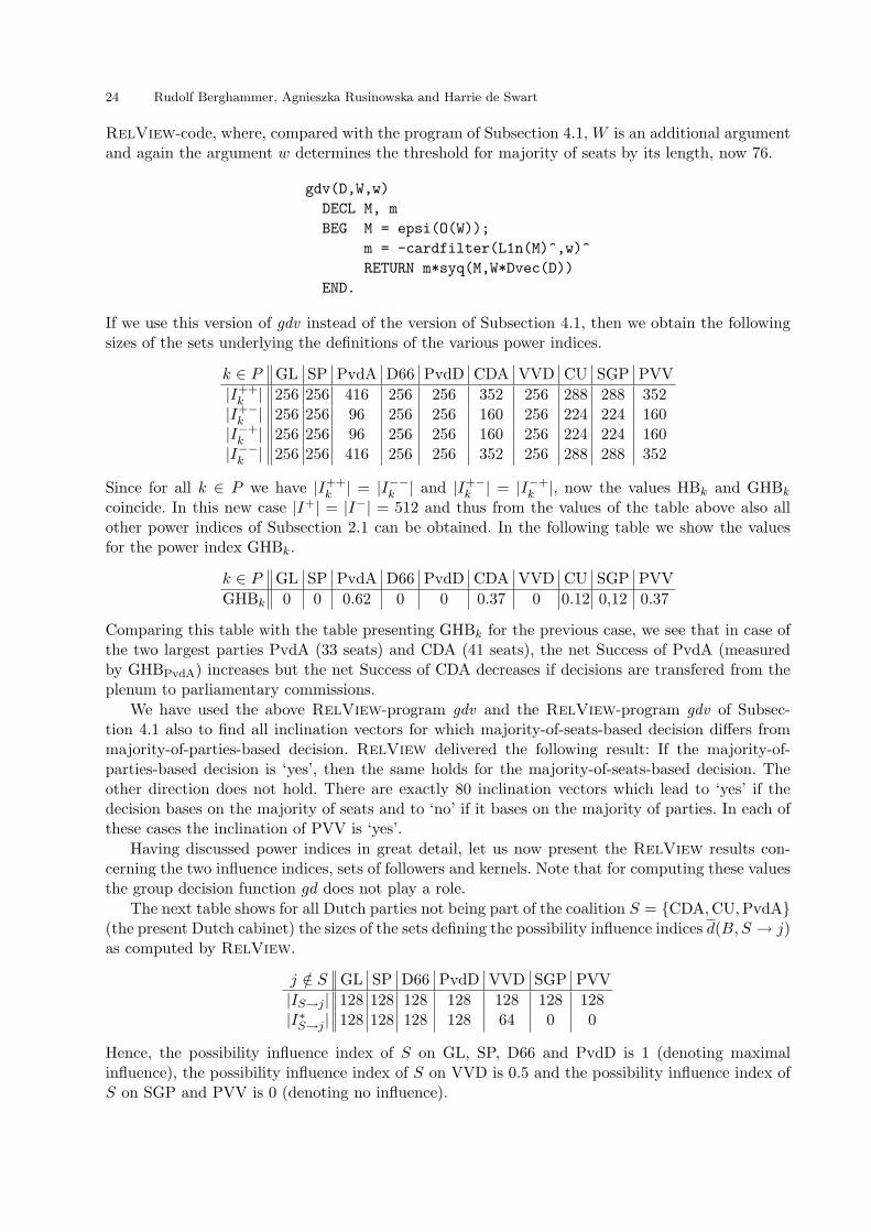
RelView-code, where, compared with the program of Subsection 4.1, W is an additional argumentand again the argument w determines the threshold for majority of seats by its length, now 76.

gdv(D,W,w)

DECL M, m

BEG M = epsi(O(W));

m = -cardfilter(L1n(M)^,w)^

RETURN m*syq(M,W*Dvec(D))

END.

If we use this version of gdv instead of the version of Subsection 4.1, then we obtain the followingsizes of the sets underlying the definitions of the various power indices.


|I++k | 256 256 416 256 256 352 256 288 288 352

|I+−k | 256 256 96 256 256 160 256 224 224 160

|I−+k | 256 256 96 256 256 160 256 224 224 160

|I−−k | 256 256 416 256 256 352 256 288 288 352

Since for all k ∈ P we have |I++k | = |I−−

k | and |I+−k | = |I−+

k |, now the values HBk and GHBk

coincide. In this new case |I+| = |I−| = 512 and thus from the values of the table above also allother power indices of Subsection 2.1 can be obtained. In the following table we show the valuesfor the power index GHBk.


GHBk 0 0 0.62 0 0 0.37 0 0.12 0,12 0.37

Comparing this table with the table presenting GHBk for the previous case, we see that in case ofthe two largest parties PvdA (33 seats) and CDA (41 seats), the net Success of PvdA (measuredby GHBPvdA) increases but the net Success of CDA decreases if decisions are transfered from theplenum to parliamentary commissions.

We have used the above RelView-program gdv and the RelView-program gdv of Subsec-tion 4.1 also to find all inclination vectors for which majority-of-seats-based decision differs frommajority-of-parties-based decision. RelView delivered the following result: If the majority-of-parties-based decision is ‘yes’, then the same holds for the majority-of-seats-based decision. Theother direction does not hold. There are exactly 80 inclination vectors which lead to ‘yes’ if thedecision bases on the majority of seats and to ‘no’ if it bases on the majority of parties. In each ofthese cases the inclination of PVV is ‘yes’.

Having discussed power indices in great detail, let us now present the RelView results con-cerning the two influence indices, sets of followers and kernels. Note that for computing these valuesthe group decision function gd does not play a role.

The next table shows for all Dutch parties not being part of the coalition S = {CDA, CU, PvdA}(the present Dutch cabinet) the sizes of the sets defining the possibility influence indices d(B, S → j)as computed by RelView.

j /∈ S GL SP D66 PvdD VVD SGP PVV

|IS→j | 128 128 128 128 128 128 128|I∗S→j | 128 128 128 128 64 0 0

Hence, the possibility influence index of S on GL, SP, D66 and PvdD is 1 (denoting maximalinfluence), the possibility influence index of S on VVD is 0.5 and the possibility influence index ofS on SGP and PVV is 0 (denoting no influence).


The results for the certainty influence indices of the present cabinet on the remaining partiesare as follows. For j being GL, SP, D66 or PvdD, from the 128 inclination vectors of I∗S→j exactlytwo show for all parties outside S an inclination that is different from the inclination of S. Hence,in these cases the certainty influence index is 1. None of the 64 inclination vectors of I∗

S→VVD hasthis property, so the certainty influence index of S on VVD is 0. That the certainty influence indexof S on the remaining parties SGP and PVV is 0 follows from |I∗S→j | = 0 for j ∈ {SGP, PVV}.

Let us, finally, present the results concerning the set of followers and kernels. We obtained withthe help of the RelView tool that

{GL,SP,PvdA,D66,PvdD,CDA,CU}

is the set of the seven followers of the present cabinet S, and that the set of singleton sets

{{PvdA}, {CDA}, {CU}, {SGP}, {PVV}}

is the kernel of the influence function induced by the above dependency graph and both influencerules we have considered in Subsection 2.3.

6 Conclusions

The present paper disseminates part of our results on applications of relation algebra and the KielRelView tool to Game Theory and Social Choice Theory. In our previous works [7, 8], we presentedsuch applications to coalition formation, where with the help of relation algebra and RelView theset of all feasible stable governments has been determined. In the present paper, we apply relationalgebra and RelView to network formation, i.e., to compute some measures of players’ strength,like power, success, and influence, in a network.

What we particularly like in this approach is its usefulness with respect to applying the tools toorganizations and trend-setter structures with a larger number of players. One of the straightforwardideas is to apply the measures calculated by RelView to parliaments. This is what we presentedin the previous section, where an application of the tools in question to the Dutch parliamentis delivered. For networks with more than, say 5 or 6 players, where some of the players havetrend-setters that they follow, calculating the measures and concepts of influence, like the Hoede-Bakker index, its generalization and modifications, the set of followers and the kernel of an influencefunction, is far too complicated to be done by hand due to the sizes of the sets I of inclinations. Incase of networks with, say, 25 players, even a naive Boolean vector approach within a conventionalprogramming language like C or Java leads to serious difficulties. It is hardly to imagine to generateall the 225 = 33.554.432 Boolean column vectors of length 25 one after another and to transformthem into the corresponding decision vectors within reasonable time. Due to the very efficient BDD-implementation of relations, the RelView tool allows to do this in a very efficient and elegantway in many cases, viz. if programs essentially are described by relation-algebraic expressions anddo not use loops that range over huge sets. To give an impression of the amazing power of theBDD-implementation of relations, we want to mention that RelView needs on a Sun Fire-280Rworkstation (750 MHz, 4 GByte main memory, running Solaris) only 0.04 seconds to compute thegroup decision vector using the program gdv of Subsection 5.2. Note that the symmetric quotientsyq(M, WDvec(D)) used in gdv has type [2N ↔ 2N ]. Regarded as a Boolean matrix, this meansthat it has 2150 rows and columns.

Of course, we also are not able to compute within reasonable time with RelView the kernel ofan influence function in the case of, say again, 25 players, if we apply the program for computingsets of followers to all subsets of P , i.e., all possible column vectors Mp : P ↔1 with p : 1↔ 2P

being a row point, via a simple loop. A strategy that may help in such a situation is to estimate the


sizes of the sets of the kernel. If we are able to show by an analysis of the dependency relationships,for instance, that each set of the kernel consists of at most 3 players, then we can use the base-operation cardfilter to obtain a row vector v : 1↔ 2P that represents the set {X ∈ 2P | |X| ≤ 3}.In the case of 25 players, instead of all 33.554.432 column vectors Mp : P ↔1 we then only have toloop through the

∑3m=0

(

25m

)

= 14.426 possible row vectors Mp with the row point p contained in v.A further advantage of the approach of the present paper is that, because of the concise form of

the RelView-programs and the expressiveness of the relation-algebraic language, the combinationof both tools additionally allows to experiment with given concepts and concepts being still underdevelopment without having a large overhead and, furthermore, to animate computations andto visualize their results. There are many more possibilities to combine relation algebra and Rel-

View to investigate and solve problems from Game Theory and Social Choice Theory. One of themcould be an application of the tools in question to bargaining theory, in particular, to determiningsolutions of bargaining games.

Acknowledgement. We like to thank Adrian Van Deemen for his suggestions concerning theexample based on the Dutch Parliament and Stefan Bolus for his further development of Rel-

View.

References

[1] J. Banzhaf, Weighted voting doesn’t work: a mathematical analysis, Rutgers Law Review 19,317-343 (1965)

[2] R. Behnke, R. Berghammer, E. Meyer and P. Schneider, RelView — A system for calculationwith relations and relational programming, In: E. Astesiano (ed.), Proc. Conf. “FundamentalApproaches to Software Engineering (FASE ’98)”, LNCS 1382, Springer, 318-321 (1998)

[3] R. Berghammer and T. Hoffmann, Modelling sequences within the RelView system, Journalof Universal Computer Science 7, 107-123 (2001)

[4] R. Berghammer, B. Karger von and C. Ulke, Relation-algebraic analysis of Petri nets withRelView, In: T. Margaria and B. Steffen (eds.), Proc. 2nd Workshop “Tools and Applicationsfor the Construction and Analysis of Systems (TACAS ’96)”, LNCS 1055, Springer, 49-69(1996)

[5] R. Berghammer, B. Leoniuk and U. Milanese, Implementation of relational algebra using binarydecision diagrams, In: H. Swart de (ed.), Proc. 6th Int. Workshop “Relational Methods inComputer Science”, LNCS 2561, Springer, 241-257 (2002)

[6] R. Berghammer, Relation-algebraic computation of fixed points with applications, Journal ofLogic and Algebraic Programming, 66, 112-126 (2006)

[7] R. Berghammer, A. Rusinowska and H. Swart de, Applying relational algebra and RelView tocoalition formation, European Journal of Operational Research 178/2, 530-542 (2007)

[8] R. Berghammer, A. Rusinowska and H. Swart de, An interdisciplinary approach to coalitionformation, European Journal of Operational Research 195, 487-496 (2009)

[9] R. Berghammer, G. Schmidt and M. Winter, RelView and Rath – Two systems for dealingwith relations, In: [49], 1-16 (2003)

[10] S.J. Brams, W.F. Lucas and P.D. Straffin, Political and Related Models, Volume 2 in seriesModels in Applied Mathematics, New York: Springer (1982)

[11] C. Brink, W. Kahl and G. Schmidt (eds.), Relational Methods in Computer Science, Advancesin Computing Science, Springer (1997)

[12] J.S. Coleman, Control of collectivities and the power of a collectivity to act, In: Lieberman,Gordon and Breach Social Choice, London (1971)

[13] J.S. Coleman, Individual Interests and Collective Action: Selected Essays, Cambridge Univer-sity Press (1986)


[14] J. Deegan and E.W. Packel, A new index of power for simple n-person games, InternationalJournal of Game Theory 7, 113-123 (1978)

[15] A. Deemen van, Dominant players and minimum size coalitions, European Journal of PoliticalResearch 17, 313-332 (1989)

[16] A. Deemen van, Coalition formation in centralized policy games, Journal of Theoretical Politics3, 139-161 (1991)

[17] A. Deemen van, Coalition Formation and Social Choice, Boston: Kluwer Academic Publishers(1997)

[18] P. Dubey and L.S. Shapley, Mathematical properties of the Banzhaf power index, Mathematicsof Operations Research 4, 99-131 (1979)

[19] E. Einy, On connected coalitions in dominated simple games, International Journal of GameTheory 14, 103-125 (1985)

[20] D.S. Felsenthal and M. Machover, The Measurement of Voting Power: Theory and Practice,Problems and Paradoxes, London: Edward Elgar Publishers (1998)

[21] M. Grabisch and A. Rusinowska, Measuring influence among players with an ordered set ofpossible actions GATE Working Paper, 2008-01, GATE, Ecully, France (2008)

[22] M. Grabisch and A. Rusinowska, Influence functions, followers and command games, Submit-ted for publication (2008)

[23] M. Grabisch and A. Rusinowska, A model of influence in a social network, Theory and Decision,forthcoming (2009)

[24] M. Grabisch and A. Rusinowska, Measuring influence in command games, Social Choice andWelfare, forthcoming (2009)

[25] C. Hoede and R. Bakker, A theory of decisional power, Journal of Mathematical Sociology 8,309-322 (1982)

[26] M.J. Holler, Forming coalitions and measuring voting power, Political Studies 30, 262-271(1982)

[27] M.J. Holler and E.W. Packel, Power, luck and the right index, Journal of Economics 43, 21-29(1983)

[28] R.J. Johnston, On the measurement of power: Some reactions to Laver, Environment andPlanning A 10, 907-914 (1978)

[29] T. Konig and T. Brauninger, The inclusiveness of European decision rules, Journal of Theo-retical Politics 10, 125-142 (1998)

[30] A. Laruelle and F. Valenciano, Assessing success and decisiveness in voting situations, SocialChoice and Welfare 24, 171-197 (2005)

[31] W.F. Lucas, Measuring power in weighted voting games, In: [10], 183-238 (1982)[32] M.J. Morgan, The Modelling of governmental coalition formation: A policy-based approach

with interval measurement, Doctoral Dissertation, University of Michigan (1976)[33] G. Owen, Game Theory, San Diego: Academic Press (1995)[34] B. Peleg, Coalition formation in simple games with dominant players, International Journal

of Game Theory 10, 11-33 (1981)[35] L.S. Penrose, The elementary statistics of majority voting, Journal of the Royal Statistical

Society 109, 53-57 (1946)[36] D. Rae, Decision rules and individual values in constitutional choice, American Political Sci-

ence Review 63, 40-56 (1969)[37] P. Roozendaal van, The effect of dominant and central parties on cabinet composition and

durability, Legislative Studies Quarterly 17, 5-36 (1992)[38] P. Roozendaal van, Cabinets in Multi-Party Democracies, Amsterdam: Thesis Publishers

(1992)[39] P. Roozendaal van, Cabinets in the Netherlands (1918-1990): The importance of ‘dominant’

and ‘central’ parties, European Journal of Political Research 23, 35-54 (1993)


[40] A. Rusinowska, On the not-preference-based Hoede-Bakker index, Forthcoming in: L. Petrosjanand V. Mazalov (eds.) Game Theory and Applications, Vol. XIII, Nova Science Publishers(2008)

[41] A. Rusinowska, The Hoede-Bakker index modified to the Shapley-Shubik and Holler-Packelindices, Submitted for publication (2008)

[42] A. Rusinowska and H. Swart de, Generalizing and modifying the Hoede-Bakker index, In: [50],60-88 (2006)

[43] A. Rusinowska and H. Swart de, On some properties of the Hoede-Bakker index, Journal ofMathematical Sociology 31(4), 267-293 (2007)

[44] A. Rusinowska, H. Swart de and J.-W. Rijt van der, A new model of coalition formation, SocialChoice and Welfare 24, 129-154 (2005)

[45] A. Rusinowska, R. Berghammer, P. Eklund, J.-W. Rijt van der, M. Roubens and H. Swart de,Social software for coalition formation, In: [50], 1-30 (2006)

[46] L.S. Shapley and M. Shubik, A method for evaluating the distribution of power in a committeesystem, American Political Science Review 48, 787-792 (1954)

[47] G. Schmidt and T. Strohlein, Relations and Graphs, Discrete Mathematics for Computer Sci-entists, EATCS Monographs on Theoret. Comput. Sci., Springer (1993)

[48] P.D. Straffin, Power indices in politics, In: [10], 256-321 (1982)[49] H. Swart de, E. Orlowska, G. Schmidt and M. Roubens (eds.), Theory and Applications of

Relational Structures as Knowledge Instruments, LNCS 2929, Springer (2003)[50] H. Swart de, E. Orlowska, G. Schmidt and M. Roubens (eds.), Theory and Applications of

Relational Structures as Knowledge Instruments II, LNAI 4342, Springer (2006)

applying relation algebra and relview to measures in a - hal-shs

Documents