approach based on minimal coordinates
TRANSCRIPT
1
GraSMech – Multibody 1
Approach based on
Minimal coordinates
Prof. O. Verlinden
Faculté polytechnique de Mons
GraSMech course 2009-2010
Computer-aided analysis of rigid
and flexible multibody systems
GraSMech – Multibody 2
Modelling steps
� Choose the configuration parameters (q)
� Set up the kinematics: express position, velocity and
acceleration (rotational and translational) of each
body in terms of q and its first and second time
derivatives
� Express the forces in terms of q, its time derivatives
and time t
� Build the differential equations of motion
� Numerical treatment of the equations
GraSMech – Multibody 3
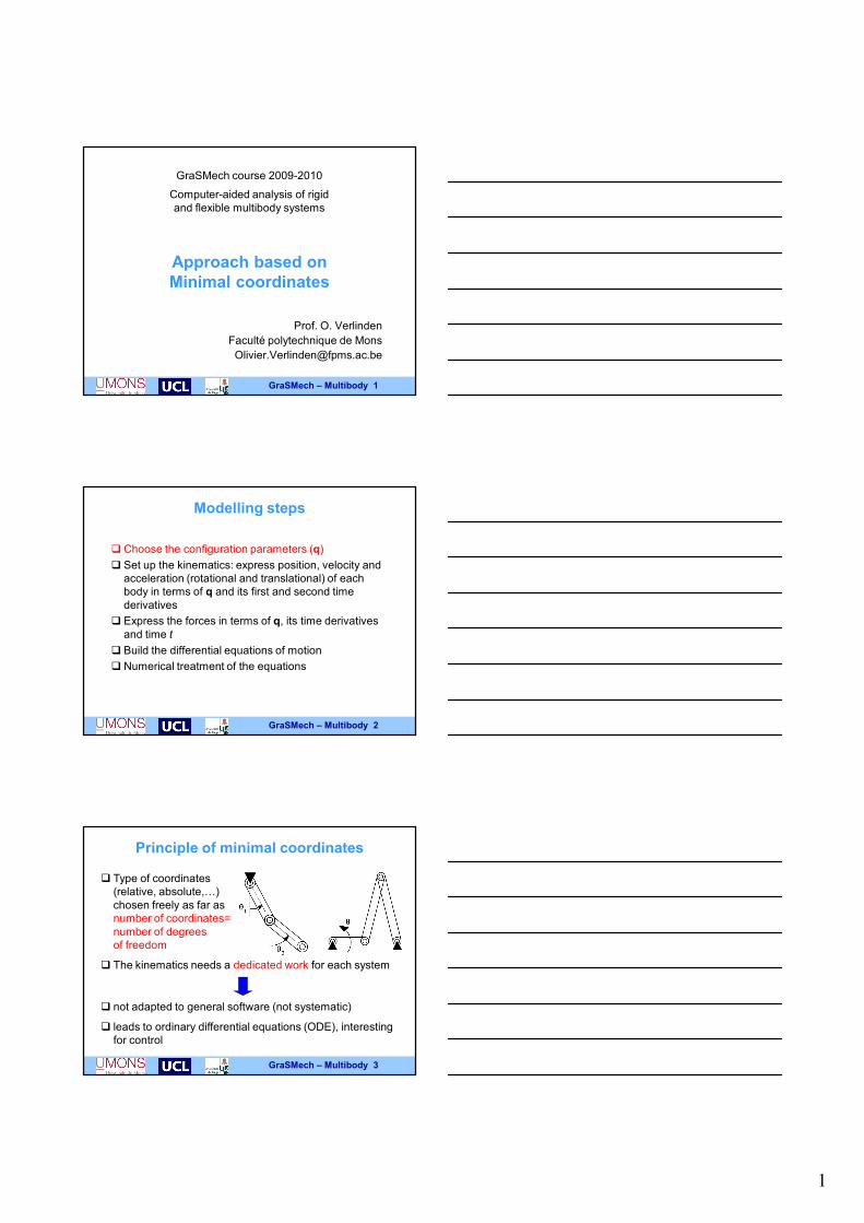
Principle of minimal coordinates
� Type of coordinates
(relative, absolute,…)
chosen freely as far as
number of coordinates=
number of degrees
of freedom
� The kinematics needs a dedicated work for each system
� not adapted to general software (not systematic)
� leads to ordinary differential equations (ODE), interesting
for control

2
GraSMech – Multibody 8
Modelling steps
� Choose the configuration parameters (q)
� Set up the kinematics: express position, velocity and
acceleration (rotational and translational) of each
body in terms of q and its first and second time
derivatives
� Express the forces in terms of q, its time derivatives
and time t
� Build the differential equations of motion
� Numerical treatment of the equations
GraSMech – Multibody 9
The need for a geometrical formalism
Tool needed to express position and orientation of a body, through a coordinate system (or frame) attached to the body
global reference
frame
body
reference
frame
(center of
mass)
secondary
body
frame
For body i -> homogeneous transformation matrix T0,i
GraSMech – Multibody 10
Vectors and coordinate systems
Tool needed to manipulate vectors (velocities, forces,
accelerations,...) in different coordinate systems

3
GraSMech – Multibody 11
Position vector of a point
GraSMech – Multibody 12
Homogeneous transformation matrices
GraSMech – Multibody 13
Examples of matrices
� Displacement without rotation
� Rotation about X axis

4
GraSMech – Multibody 14
Examples of matrices
� Rotation about Z axis
� Rotation about a unit vector n
GraSMech – Multibody 15
Switching between coordinate systems
Postion vectors relative to different coordinate systems
are linked by transformation matrices
The position of a point P of body i is easily
expressed from its local coordinates and T0,i
GraSMech – Multibody 18
Homogeneous transformation matrices are particularly interesting along kinematic chains (robotics)
Multiplication of position matrices
A complex matrix is built from the multiplication of
elementary matrices (rotation or translation)

5
GraSMech – Multibody 21
Position, velocity and parameters
Situation of each body expressed in terms of q
General form of velocity
GraSMech – Multibody 22
Kinematic matrices
� Velocities can be expressed in matrix form
� as well as accelerations
GraSMech – Multibody 23
Example: double pendulum

6
GraSMech – Multibody 24
Example: double pendulum
GraSMech – Multibody 25
Example: double pendulum
GraSMech – Multibody 26
Global kinematics
� Kinematics of body i
� Kinematics of secondary frames

7
GraSMech – Multibody 29
Modelling steps
� Choose the configuration parameters (q)
� Set up the kinematics: express position, velocity and
acceleration (rotational and translational) of each
body in terms of q and its first and second time
derivatives
� Express the forces in terms of q, its time derivatives
and time t
� Build the differential equations of motion
� Numerical treatment of the equations
GraSMech – Multibody 30
Expression of forces
For each body i, we need
� The resultant force of all applied forces exerted on
body i
� The resultant moment of all applied forces exerted on
body i, with respect to center of mass
GraSMech – Multibody 31
Force elements - examples
� Spring
(stiffness k and
rest length l0)
� Damper (damping
coefficient c)

8
GraSMech – Multibody 32
Example: double pendulum
The only applied force is the
gravity
GraSMech – Multibody 35
Modelling steps
� Choose the configuration parameters (q)
� Set up the kinematics: express position, velocity and
acceleration (rotational and translational) of each
body in terms of q and its first and second time
derivatives
� Express the forces in terms of q, its time derivatives
and time t
� Build the differential equations of motion
� Numerical treatment of the equations
GraSMech – Multibody 36
Equations of motion
How to get (in a systematic way now) the equations of
motion from
�Kinematics
�Applied efforts on each body
The theorem of virtual power (d’Alembert) is particularly
well suited
for any virtual motion and even
for any admissible virtual motion (principle of VP)

9
GraSMech – Multibody 37
Virtual power of applied forces
� Kinematically admissible motion
as kinematic step includes all the joints
� Power developed by applied forces
GraSMech – Multibody 38
Virtual power of inertia forces
� Power developed by inertia forces
with mi and ΦGi the mass and tensor matrix of body i
GraSMech – Multibody 39
Equations of motion
Globally, the expression
becomes

10
GraSMech – Multibody 40
Equations of motion
� Equations of motion=second-order ordinary differential equations (ODE)
� with the mass matrix
� the Coriolis and centrifugal terms
� and the contribution of applied forces
GraSMech – Multibody 41
Equivalent vector form
Equations of motion can also be obtained from partial
velocities
with for example for the mass matrix
GraSMech – Multibody 42
Applicability of minimal coordinates
Equations of motion can be written from kinematics and
applied efforts !
But ... is the method applicable in practice ?
Yes -> Team of Prof. Manfred Hiller (University of
Duisburg, Germany), A. Keczkemethy,
M. Anantharaman

11
GraSMech – Multibody 43
Practical implementation
� Classical organization of a MBS software
Application 1
Generals
olver
Results 1
Application 2
Application 3
Results 2
Results 3
Data
files
� Organization with minimal coordinates
General
library
Results 1Dedicated program 1
Results 2
Results 3
Dedicated program 2
Dedicated program 3
GraSMech – Multibody 44
Components of the library
� Routines to express motion (composition of
movements along a kinematic chain)
� Routines to solve constraints
� Routines to express forces (springs, dampers, tires,
contact,…)
� Routines to build equations of motion from kinematics
and applied forces
� Routines for the numerical treatment of equations of
motion (integration, static equilibrium, linearization,
computation of poles,…)
GraSMech – Multibody 45
Principle for generalization (Hiller)
Inside a loop, the motion is described in terms of
minimal coordinates (loop=kinematic transformer)
Independent configuration parameters
Dependent conf. parameters
Expression of motion
Solving of constraints
Basic ideas: constraints solved in advance and by loops

12
GraSMech – Multibody 46
Generalization - example
Example: slider-crank mechanism
And so on for velocities and accelerations !!
GraSMech – Multibody 47
Kinematic transformer (Hiller)
Loop=kinematic transformer
Different strategies to solve loops: typical pair of joints,
minimal polynomial equation, automatic gneration of
closed-form solutions
GraSMech – Multibody 48
Industrial example
Not limited to simplistic systems !
30 bodies
40 joints
13 loops
25 dof

13
GraSMech – Multibody 49
Other implementation: EasyDyn
GraSMech – Multibody 50
Components of EasyDyn
GraSMech – Multibody 51
Using EasyDyn (C++ only)
The user must a provide a C++ program with
� Routine SetInertiaData() specifying the inertia properties of all bodies
� Routine ComputeMotion() implementing
� Routine AddAppliedEfforts() describing the efforts on each body (eventually with the help of available routines)
� A main routine for initialization and call of integration routines
The user can rely on the vec module for kinematics and efforts

14
GraSMech – Multibody 52
CAGeM
GraSMech – Multibody 53
Using EasyDyn with CAGeM
Mupad script with
� Dimensions
� Inertia properties
� Kinematics (position)
� Gravity
� Initial conditions
� options
Core C++ program
� Kinematics (velocity
and acceleration)
� External forces
(gravity only)
� Typical simulation
(time integration)
CAGeM
Body i: TOG[i]=Trotz(q[0])*Tdisp(q[1],0,0)…
q[j]= configuration parameter
Number of configuration parameters=number of degrees
of freedom (minimal coordinates- no constraints)
GraSMech – Multibody 54
Using EasyDyn with CAGeM (2)
Core C++ program
� Kinematics (velocity
and acceleration)
� External forces
(gravity only)
� Time integration
Add other forces
� Available routines
(spings, dampers,…)
� Vector library
Add other differential
equations (electrical,
pneumatic,
hydraulic,…)
Adapt simulation (static
equilibrium,
poles,discrete-time
operations)

15
GraSMech – Multibody 55
Double pendulum in MuPAD
GraSMech – Multibody 56
Double pendulum in MupAD
GraSMech – Multibody 57
Some interesting features of CAGeM

16
GraSMech – Multibody 58
Slider-crank mechanism
GraSMech – Multibody 59
Robot
3D doesn’t make any difference !
GraSMech – Multibody 60
Interest of CAGeM

17
GraSMech – Multibody 61
Efforts of actuators
vectors
action
reaction
GraSMech – Multibody 62
Walking robot AMRU5
AMRU: Autonomy of Mobile Robots in Unstructued
environments
AMRU5: hexapod robot built by RMA, ULB and VUB
•18 degrees of freedom
•hierarchical control:
central controller
+one controller per leg
(Microchip PIC)
•about 30 kg
•Diameter about 1 m
GraSMech – Multibody 63
Leg of AMRU5
Mechanism of the leg=pantograph
Horizontal and vertical motions of the
foot are driven independently
-> gravitationally decoupled actuation

18
GraSMech – Multibody 64
Mechanics of the leg
Nut-screw
Motor-gearbox-encoder
Axis of rotation
GraSMech – Multibody 65
Model of AMRU5
� Contact with the ground introduced as external forces
� Total of 24 degrees of freedom
T0G[0]=Tdisp(q[0],q[1],q[2])
*Trotx(q[3])*Troty(q[4])*Trotz(q[5])
GraSMech – Multibody 66
Kinematics of the pantograph
The situation of each body must be expressed from the 2
configuration parameters

19
GraSMech – Multibody 67
Kinematics of the pantograph
GraSMech – Multibody 68
Summary of the model
� 49 bodies
� The central body
� 8 bodies per leg (support part, 4 leg members and 3 rotors)
� 24 configuration parameters(and second-order differentialequations) for the mechanical part
� PID Controllers
� 36 differential equations in continuous time (test only)
� Algebraic expressions in discrete time (actual controller)
� First-order model of DC motors
� Contact force derived from relative motion with respect to the ground (nonlinear elastic with damping)
Input of the simulation: targets of the controllers
GraSMech – Multibody 69
Interest of the model
The main interest of the model is to improve the gait
generation => softer and less energy consumption

20
GraSMech – Multibody 70
Let’s have it walk !
Bad gait Good gait
Climbing
GraSMech – Multibody 71
Example: human walking
Interest of EasyDyn in Biomechanics
� Particular kinematics (not classical joints)
� Particular forces
�Contact forces (foot-ground)
�Resistive joint torques
�Muscle modelling
Rustin Cédric, F.S.R.-FNRS PhD student
University of Mons (UMONS)
7000 Mons (Belgium)
GraSMech – Multibody 72
Human lower limbs and walking process
� Kinematics : Delp's model
� 14 bodies :
− Torso-head
− Pelvis
− 2 femurs
− 2 patellas
− 2 tibias-fibulas
− 2 talus
− 2 calcaneus
− 2 sets of toes

21
GraSMech – Multibody 73
Human lower limbs and walking process
� Kinematics : Delp's model
� 11 joints and 23 dof :− 6 for the pelvis
− 3 orientation angles for the torso-head
wrt the pelvis
− 3 orientation angles for each thigh
wrt the pelvis
− the knee angle for each calf
wrt each thigh
− the ankle angle for each talus
wrt each calf
− the angle for each calcaneus
wrt each talus
− the angle for each set of toes
wrt to each calcaneus
GraSMech – Multibody 74
Human lower limbs and walking process
Human articulations are not classical
mechanical joints
For instance, for the femur-(tibia-fibula)
joint (one dof joint)TrefG[R_TIBIAFIBULA]:=
…
*Tdisp(g5_(q[R_KNEE_ang]),
g6_(q[R_KNEE_ang]),
R_tibia_fibula_kinematicstranslation_z)
*Trotz(q[R_KNEE_ang])
*…
GraSMech – Multibody 75
Human lower limbs and walking process
Passive joint moments: results form
the resistance and damping
generated by the skin, soft
tissues, cartilages, muscles and
tendons wrapping the joint.
Amankwah's model: passive
moment described by a
differential equation

22
GraSMech – Multibody 76
Human lower limbs and walking process
Muscles (particular actuator)
� 88 muscles for the 2 lower limbs
� Can be modelled with the virtual
muscle Brown and Loeb’s models
6 ODE's per muscle
� the excitation and activation
processes
� the F-L and F-V filters
� the properties of the slow and
fast fiber types
� the yield and sag phenomena
� ...
GraSMech – Multibody 77
Human lower limbs and walking process
Foot-ground contacts: 6 ellipsoids of contact
Non linear contact force expressed in terms of penetration
and penetration rate
GraSMech – Multibody 78
Present work: dynamic simulation of walking
Presently input data = joint angles and velocities
Soon (hopefully) input data = muscles activation history
Input data must be adapted by optimzation for a stable
walking

23
GraSMech – Multibody 79
Conclusion
� The approach based on minimal coordinates requires
a dedicated kinematics from the user
�Advantage: freedom
�Drawback: laborious, risk of mistakes
� It is not limited to simplistic systems (with a good
library)
� No constraints in the equations of motion
� It is well adapted to education