aquasim manual
TRANSCRIPT

AQUASIM 2.0 { User Manual
Computer Program
for the Identi�cation and Simulation
of Aquatic Systems
Peter Reichert
Swiss Federal Institute for EnvironmentalScience and Technology (EAWAG)
CH - 8600 D�ubendorfSwitzerland
September 1998
ISBN: 3-906484-16-5

i
Preface
The ideas for the realization of the program AQUASIM described in this manual grew from
the experiences made in a lot of interdisciplinary studies at the Swiss Federal Institute
for Environmental Science and Technology (EAWAG), CH-8600 D�ubendorf, Switzerland,
in which I have been involved. It is not possible to mention all persons, who contributed
with the discussion of their data interpretation and modelling problems to the concepts
of this program.
By far the largest in uence to the concepts of this program are due to Oskar Wanner
and J�urg Ruchti. The large number of common data analysis and parameter estimation
projects with Oskar Wanner let us recognise the usuefulness of a more universal program
than those available at that time. J�urg Ruchti raised my interest in object-oriented pro-
gramming and for the programming language C++ that was used for the implementation.
The discussions with him signi�cantly improved the design of the program. The realization
of the program BIOSIM speci�cally designed for bio�lm modelling together with Oskar
Wanner and J�urg Ruchti had also an important in uence on this project. AQUASIM
includes the functionality of BIOSIM as a special case.
Version 1.0 of the AQUASIM was documented in a technical report that contained
information on modeling in general, on the selection of program tasks, on numerical algo-
rithms, on object-oriented implementation concepts and on examples of program applica-
tion (Reichert, 1994b). The user manual with a brief tutorial was given in the appendix
of this report. Because of the addition of a new variable type (probe variable), of several
new compartments (advective-di�usive reactor, saturated soil column, lake), signi�cant
extensions of the bio�lm reactor compartment, and several new features for simulation
and batch processing, this user manual got out of date. In addition, a new user interface
for the most widely used platform (Microsoft Windows), made the use of the program
more comfortable. Because most users are only interested in the use of the program and
not in the implementation concepts, I decided to write a new user manual and, as a sep-
arate volume, a new, more attractive tutorial (Reichert, 1998). In this new user manual
the equations solved by the program are given in the same chapter as the program use is
described. This should facilitate the understanding of what the program does. For persons
interested in numerical methods or in the implementation concepts, the technical report
is still the most complete source of information. In addition, a brief description of the
major program features (Reichert, 1994a) and a summary of the implementation concepts
(Reichert, 1995) are also available.
I would like to thank J�urg Ruchti for the implementation of the formula variables and
the plotting facilities, and Werner Simon for the realization of the saturated soil column
compartment. Furthermore, Oskar Wanner contributed to the design of the extensions
of the bio�lm compartment, Claudia Fesch and Stefan Haderlein to the design of the

ii
soil column compartment, and Gerrit Goudsmit and Johny W�uest to the design of the
lake compartment. G�erard Mohler, Bouziane Outiti and Raoul Scha�ner gave support
in solving technical problems involving di�erent hardware platforms, and Martin Omlin
introduced me into the LATEX system used for typesetting this manuscript. In addition,
many program users gave hints on program errors and on possibilities for improvements.
Most parts of this manual have been newly written. I apologize for all errors that it may
contain. If you detect errors or unclear paragraphs, please send a note to [email protected].
I will improve this manual during the next years and try to eliminate as many errors as
possible.
Peter Reichert, September 1998

Contents
1 Introduction 1
2 File Handling 7
3 Model Formulation 9
3.1 Variables . . . . . . . . . . . . . . . . . . . . . . . . . . . . . . . . . . . . . 12
3.1.1 State Variables . . . . . . . . . . . . . . . . . . . . . . . . . . . . . . 14
3.1.2 Program Variables . . . . . . . . . . . . . . . . . . . . . . . . . . . . 15
3.1.3 Constant Variables . . . . . . . . . . . . . . . . . . . . . . . . . . . . 17
3.1.4 Real List Variables . . . . . . . . . . . . . . . . . . . . . . . . . . . . 18
3.1.5 Variable List Variables . . . . . . . . . . . . . . . . . . . . . . . . . . 21
3.1.6 Formula Variables . . . . . . . . . . . . . . . . . . . . . . . . . . . . 23
3.1.7 Probe Variables . . . . . . . . . . . . . . . . . . . . . . . . . . . . . . 26
3.2 Processes . . . . . . . . . . . . . . . . . . . . . . . . . . . . . . . . . . . . . 27
3.2.1 Dynamic Processes . . . . . . . . . . . . . . . . . . . . . . . . . . . . 28
3.2.2 Equilibrium Processes . . . . . . . . . . . . . . . . . . . . . . . . . . 30
3.3 Compartments . . . . . . . . . . . . . . . . . . . . . . . . . . . . . . . . . . 32
3.3.1 Mixed Reactor Compartment . . . . . . . . . . . . . . . . . . . . . . 34
3.3.2 Bio�lm Reactor Compartment . . . . . . . . . . . . . . . . . . . . . 41
3.3.3 Advective-Di�usive Reactor Compartment . . . . . . . . . . . . . . . 59
3.3.4 Saturated Soil Column Compartment . . . . . . . . . . . . . . . . . 70
3.3.5 River Section Compartment . . . . . . . . . . . . . . . . . . . . . . . 85
3.3.6 Lake Compartment . . . . . . . . . . . . . . . . . . . . . . . . . . . . 98
3.4 Links . . . . . . . . . . . . . . . . . . . . . . . . . . . . . . . . . . . . . . . . 125
3.4.1 Advective Link . . . . . . . . . . . . . . . . . . . . . . . . . . . . . . 126
3.4.2 Di�usive Link . . . . . . . . . . . . . . . . . . . . . . . . . . . . . . . 129
3.5 Numerical Parameters . . . . . . . . . . . . . . . . . . . . . . . . . . . . . . 132
3.6 Deleting Calculated States . . . . . . . . . . . . . . . . . . . . . . . . . . . . 135
4 Simulation and Data Analysis 137
4.1 Simulation . . . . . . . . . . . . . . . . . . . . . . . . . . . . . . . . . . . . . 138
4.2 Sensitivity Analysis . . . . . . . . . . . . . . . . . . . . . . . . . . . . . . . . 144
4.3 Parameter Estimation . . . . . . . . . . . . . . . . . . . . . . . . . . . . . . 151
5 Visualization of Results 161
iii

iv CONTENTS
6 Appendix 171
6.1 Character Interface Version . . . . . . . . . . . . . . . . . . . . . . . . . . . 171
6.2 Batch Version . . . . . . . . . . . . . . . . . . . . . . . . . . . . . . . . . . . 173
6.3 Troubleshooting . . . . . . . . . . . . . . . . . . . . . . . . . . . . . . . . . . 176
6.3.1 Problem Self-Diagnosis . . . . . . . . . . . . . . . . . . . . . . . . . . 177
6.3.2 Finding Help in the AQUASIM User Group . . . . . . . . . . . . . . 187
6.3.3 Reporting Program Bugs and Suggestions for Improvements . . . . . 188

Chapter 1
Introduction
The program AQUASIM was designed for the identi�cation and simulation of aquatic
systems in the laboratory, in technical plants and in nature. This user manual describes the
equations solved by this program, the methods of systems analysis that are available and
program handling. An additional document contains a series of extensively documented
tutorial examples (Reichert, 1998). A brief survey on the capabilities of version 1.0 of the
program (Reichert, 1994a) as well as a description of program implementation techniques
(Reichert, 1995) can be found in scienti�c journals. Finally, there exists an extensive
technical report on all aspects of version 1.0 of the program (Reichert, 1994b). Examples
of program applications can be found in the following publications:
Mixed reactor systems: (von Schulthess et al., 1994; Wild et al.,
1994; Reichert et al., 1995; Siegrist et al.,
1995; Wild et al., 1995; von Schulthess and
Gujer, 1996; Uehlinger et al., 1996; Kuba
et al., 1996; Murnleitner et al., 1997; Novack
and Sigg, 1997; Glod et al., 1997a; Musvoto
et al., 1997; Eisenbeis et al., 1997; Peeters
et al., 1997; Glod et al., 1997b; Filipe and
Daigger, 1997).
Bio�lm systems: (Wanner et al., 1994; Janning et al., 1995;
Horn and Hempel, 1995; Wanner et al., 1995;
Wanner, 1996; Wanner and Reichert, 1996;
Reichert and Wanner, 1997; Vrany et al.,
1997; Horn and Hempel, 1997; Mirpuri et al.,
1997; Arcangeli and Arvin, 1997b; Arcan-
geli and Arvin, 1997a; Sanderson and Stew-
art, 1997; Suci et al., 1998; Beaudoin et al.,
1997).
Advective-di�usive reactor systems: (von Gunten et al., 1997).
Saturated soil column systems: (Simon et al., 1997; Fesch et al., 1998b; Fesch
et al., 1998a).
1

2 CHAPTER 1. INTRODUCTION
River systems: (Londong et al., 1994; Albrecht et al., 1995;
Jancarkova et al., 1997; Maryns and Bauwens,
1997).
Lake systems: {.
An updated list of references of AQUASIM applications can be found at the EAWAG
home page at http://www.eawag.ch.
Program Design
Comparison of measurements with model calculations is the most important method of
testing theories in the natural sciences. Most mathematical models of environmental
systems consist of a set of nonlinear ordinary or partial di�erential equations. A com-
puter program which solves these equations numerically is usually required for calculating
model predictions. Most programs available for this purpose can be put into one of three
categories: universal simulation software; environmental simulation programs; and sys-
tem identi�cation programs. Universal simulation software is very exible with regard to
model formulation, but it is di�cult to use, especially for non-specialists. Environmental
simulation programs are much easier to handle, but they usually implement a speci�c
model selected by the designer of the program. This makes their use for the comparison
of di�erent models impossible. Finally, system identi�cation programs provide important
tools for model comparison and parameter estimation, but the class of models considered
in these programs is in most cases restricted to linear or algebraic models, and models
cannot be formulated in a way familiar to environmental scientists. Although the clas-
si�cation of simulation programs into these categories is not strict and there are also (a
few) programs that cover tasks belonging to more than one of these categories, a univer-
sal identi�cation and simulation program is not yet available. The intention behind
the design of the program AQUASIM was to provide a more universal iden-
ti�cation and simulation tool for a class of aquatic systems important in the
environmental sciences. An additional important program design criterion
was user-friendliness, which was achieved not only by providing a graphical
user interface, but also by utilizing a communication "language" familiar to
environmental scientists. AQUASIM is extremely exible in allowing the user
to specify transformation processes, and, in addition to perform simulations
for the user-speci�ed model, it provides elementary methods for parameter
identi�ability analysis, for parameter estimation and for uncertainty analysis.
Version 1.0 of AQUASIM was developed in the years 1991-1994 in the Computer and
Systems Sciences department of the Swiss Federal Institute for Environmental Science
and Technology (EAWAG), CH-8600 D�ubendorf, Switzerland, and it is maintained and
extended since then. The program was designed mainly for internal use in research and
teaching, but is also available to the public. Information on the newest developments of
AQUASIM can be found at the EAWAG home page at http://www.eawag.ch.
Program Tasks
AQUASIM is a program for the identi�cation and simulation of aquatic systems. It per-
forms the four tasks of
� simulation,

3
� identi�ability analysis,
� parameter estimation,
� uncertainty analysis.
Due to the similarity of the mathematical techniques involved, identi�ability and uncer-
tainty analyses are combined to yield sensitivity analysis.
The �rst task of AQUASIM is to allow the user to perform model simulations. By
comparing calculated results with measured data, such simulations reveal whether certain
model assumptions are compatible with measured data. The existence of systematic devi-
ations between calculations and measurements provides a hint that additional important
processes may have to be considered, or corrections must be made in the way processes are
formulated. AQUASIM allows the user to change model structure and parameter values
easily.
AQUASIM's second task is to perform sensitivity analyses with respect to a set of
selected variables. This feature allows the user to calculate linear sensitivity functions of
arbitrary variables with respect to each of the parameters included in the analysis. These
sensitivity functions help in assessing the identi�ability of model parameters (identi�ability
analysis). Furthermore, the derivatives calculated in sensitivity analyses allow the user to
estimate the uncertainty in any variable according to the linear error propagation formula.
The calculation of the contribution of each parameter to the total uncertainty facilitates
the detection of major sources of uncertainty (uncertainty analysis).
The third important task of AQUASIM is to perform parameter estimations au-
tomatically for a given model structure using measured data. This is not only impor-
tant for obtaining neutral estimates of parameters, but is also a main prerequisite for
e�ciently comparing di�erent models. Several calculations, each of them describing a
single experiment with the possibility for several target variables, as well as universal
and experiment-speci�c model parameters, can be combined to a single parameter estima-
tion process. The quantitative measure of the deviation between model calculations and
measurements, which is minimized by the parameter estimation algorithm, is useful for
statistically assessing the adequacy of the model.
User Interfaces
Three versions of the program AQUASIM with di�erent user interfaces are provided. The
window interface version, aquasimw, uses the machines own graphical user interface.
The use of this version is strongly recommended for editing models, for de�ning sensitivity
analyses and parameter estimations, for specifying plot de�nitions, for performing short
calculations and for viewing results. The second version is the character interface
version, aquasimc. This version is intended for users having a simple terminal without
graphical capabilities. It provides all features available in the window interface version
except the capability of plotting results directly on the screen (listing results and preparing
plots for printing, however, is also possible with this program version). The third version is
the batch version, aquasimb, which is designed for submitting long calculations as batch
jobs (it should be noted that simulations, and especially sensitivity analyses and parameter
estimations, may require much computation time). This version allows the user to start a
calculation for an AQUASIM system, de�ned with one of the interactive program versions,
by specifying one simple command line. It is also possible to specify a series of AQUASIM
jobs on a command �le so that the consecutive execution of calculations together with

4 CHAPTER 1. INTRODUCTION
listing and plotting results can be combined to a single batch job. In the batch version of
AQUASIM, models cannot be modi�ed.
Hardware Platforms and Operating Systems
AQUASIM is written in the standardized object oriented programming language C++.
There is a strict separation between the core program and the di�erent user interface
layers. There exist two versions of the user interface layer for the window interface version
of the program. The �rst uses a graphical user interface library, which is available for
various hardware platforms and operating systems. This program design makes AQUASIM
highly portable. A second implementation of the user interface version of the window
interface version is speci�cally designed for the Microsoft Windows operating system.
The character interface version and the batch version can be compiled on nearly any
platform and operating system without the need of special libraries. Table 1.1 gives a
survey on all currently supported computing platforms.
Program
Hardware Operating System Window System Version
w c b
Sun SparcStation Solaris 2.x OpenWindows X X XMotif 1.2 X X X
IBM RS/6000 AIX 3.2.x - - X X
HP 700 series HP-UX 9.x - - X X
DEC Alpha series VMS 6.x - - X XDEC Unix - - X X
Intel 80486/Pentium MS-DOS 5 or 6 Windows 3.1 (Win32s) X - -Windows 95 native X X XWindows NT native X X X
Apple Power Macintosh MacOS 7.x native X X X
Table 1.1: Computing platforms supported by the current AQUASIM version.
Organization of this Manual
Throughout this user manual it is assumed that the user is familiar with system speci�c
handling of menus, windows, list boxes, buttons, etc.. The description mainly concentrates
on the window interface version of the program. The functionality of the character interface
version is the same with the exception that it is not possible to plot graphics to the screen
with this program version. In section 6.1 a brief introduction to the character interface
version is given. In section 6.2 it is shown how batch jobs can be submitted.
Figure 1.1 shows the main window of AQUASIM with the header, the menu bar
and a button bar which facilitates the access to the most important menu commands
(from left to right: File!New, File!Open, File!Save, Edit!Cut (inactive), Edit-
!Copy (inactive), Edit!Paste (inactive), Edit!System, Edit!Delete States, Calc-
!Simulation, Calc!Sensitivity Analysis, Calc!Parameter Estimation, View!Re-
sults, View!Close Dialogs). The commands in the four menus File, Edit, Calc and
View are described in the chapters 2-5 of this user manual. The menu `File' (chapter 2)
is used for saving, loading and printing the current AQUASIM system, which consists of

5
Figure 1.1: Main window of AQUASIM.
the mathematical model, measured data, de�nitions of sensitivity analyses and parame-
ter estimations, plot de�nitions and calculated states. With the aid of the menu `Edit'
(chapter 3), the mathematical model and measured data can be entered and edited. The
menu `Calc' (chapter 4) is used to de�ne and perform simulations, sensitivity analyses
and parameter estimations. Finally, the menu `View' (chapter 5) is used to specify plot
de�nitions and to list and plot results. The appendix (chapter 6) contains additional
information speci�c to the di�erent program versions and some hints for troubleshooting.
How to Proceed
The following procedure is recommended for learning to use the program AQUASIM:
1. Read the introduction to this manual (chapter 1) to obtain a general idea of
program concepts and capabilities.
2. Skim over the chapters 2-5 to increase your knowledge of program concepts and
to start learning to use the program interface. If you plan to work with the
character interface version, read section 6.1 also.
3. Study the tutorial exercises described in a separate document (Reichert, 1998),
and carefully read the corresponding sections of the chapters 2-5 of this user
manual if you have problems in understanding the solutions.
4. Start using the program as a scienti�c and/or didactic tool. It may be helpful
to implement the �rst model by modifying one of the example applications or
one of the tutorial system �les instead of starting from scratch. If problems
arise, look at section 6.3 for hints on troubleshooting.

6 CHAPTER 1. INTRODUCTION
Chapter 2
File Handling
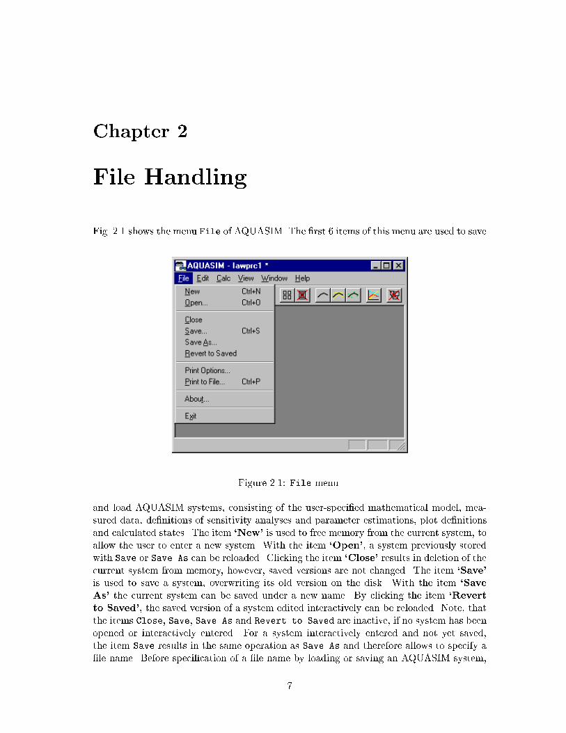
Fig. 2.1 shows the menu File of AQUASIM. The �rst 6 items of this menu are used to save
Figure 2.1: File menu.
and load AQUASIM systems, consisting of the user-speci�ed mathematical model, mea-
sured data, de�nitions of sensitivity analyses and parameter estimations, plot de�nitions
and calculated states. The item `New' is used to free memory from the current system, to
allow the user to enter a new system. With the item `Open', a system previously stored
with Save or Save As can be reloaded. Clicking the item `Close' results in deletion of the
current system from memory, however, saved versions are not changed. The item `Save'
is used to save a system, overwriting its old version on the disk. With the item `Save
As' the current system can be saved under a new name. By clicking the item `Revert
to Saved', the saved version of a system edited interactively can be reloaded. Note, that
the items Close, Save, Save As and Revert to Saved are inactive, if no system has been
opened or interactively entered. For a system interactively entered and not yet saved,
the item Save results in the same operation as Save As and therefore allows to specify a
�le name. Before speci�cation of a �le name by loading or saving an AQUASIM system,
7

8 CHAPTER 2. FILE HANDLING
the item Revert to Saved is inactive. Furthermore, as long as a loaded system is not
yet modi�ed, the items Save and Revert to Saved are inactive. AQUASIM system �les
should not be edited with other programs, because such an attempt can result in inconsis-
tent or unreadable �les. AQUASIM system �les can be transfered between all supported
platforms using text (ASCII) data transfer. The �le format is also compatible with elec-
tronic mail; mailed system �les can directly be opened on any platform together with
their mail headers. To keep a reasonable �le size, it is recommended to delete calculated
states before saving to an AQUASIM system �le that is planned to be included in a mail
message.
The menu item `Print Options' allows to select the print �le format. As shown
in Fig. 2.2, a long and a short format can be selected. In the long format, (nearly)
Figure 2.2: Dialog box for editing print options.
all user speci�cations are listed, whereas the short form allows to have a compact listing
of the most essential model elements. To facilitate program portability, the menu item
`Print to File' does not directly print the system de�nitions, but only writes them to a
text �le, the name of which can be speci�ed by the user. Such text �les have then to be
submitted to a printer by the user either directly or after loading them into an editor or a
text processing program. Printing an AQUASIM system is very useful, because the clear
arrangement of all system de�nitions facilitates checking user input or understanding the
meaning of objects loaded from an AQUASIM system �le created by someone else. Note,
however, that an AQUASIM system cannot be reloaded from a print �le.
The menu item `About' gives information on the installed program version. This
information is also written to any output �le written by AQUASIM.
Finally, clicking the menu item `Exit' results in program termination. If system de�-
nitions have been edited or if states have been calculated or deleted, the user is asked to
save the changes.
For each interactive AQUASIM session, a log �le with the name aquasim.log is written
to the startup directory of the program (in the batch version, the name of the log �le can
be speci�ed by the user). This log �le contains information on the progress of calculations.
In the case of normal program termination, the log �le can be ignored (and deleted); in
the case of problems during calculation, the information provided in the log �le may help
locating the problem. Restarting AQUASIM in the same directory as before, leads to
overwriting the old version of the log �le, so that only the log �les of the most recent
sessions (in di�erent directories) are available (unless an old log �le has been renamed).

Chapter 3
Model Formulation
In the program AQUASIM, a model consists of a system of ordinary and/or partial di�er-
ential equations and algebraic equations, which deterministically describes the behaviour
of a given set of important state variables of an aquatic system. The di�erential equations
for water ow and substance transport can be selected by the choice of environmental
or technical compartments, which can be connected by links. The source terms of these
equations, which describe the e�ect of transformation processes, can be freely speci�ed
by the user. The de�nition of such transformation processes follows closely the notation
of biochemical processes, as it is familiar to environmental scientists and engineers. The
de�nition of processes, compartments and links is done with the aid of variables, which
represent objects taking a possibly context-sensitive numerical value. Fig. 3.1 visualizes
the mutual depedencies between the four subsystems of variables, processes, compart-
ments and links. It is evident, that the variables form the basic subsystem required for
Variables
Compartments
Processes
Links
Figure 3.1: Main elements of model structure.
the formulation of processes, compartments and links. Processes must be de�ned before
they can be activated in compartments. Finally, links can be used to connect compart-
ments that are already de�ned. After a short overview of the four subsystems of the
AQUASIM model structure, in this chapter, the de�nition of objects of these subsystems
is explained in detail (sections 3.1 to 3.4). All these de�nitions together form the model
9

10 CHAPTER 3. MODEL FORMULATION
used by AQUASIM for simulation and data analysis.
The basic subsystem of the AQUASIM model structure is the system of variables.
Variables are objects which are characterized by the property of taking a numerical value.
This value may depend on the values of other variables. Six types of variables are
distinguished: State variables are used to describe properties of water or of a surface
in contact with water to be calculated by the model. Program variables make auxiliary
quantities used in the program available to the system of variables. Constant variables
and real list variables are used to provide measured quantities for use in the system
of variables. In addition, constant variables are used as model parameters in sensitivity
analyses and parameter estimations. Variable list variables and formula variables are
used to build functional relations out of other variables. Finally, probe variables make
the values of variables evaluated at a given location in a compartment globally available.
The system of variables serves as a pool of variables for the formulation of the other
subsystems.
The next subsystem of the AQUASIM model structure is the system of processes.
Two types of processes are distinguished: Dynamic processes implement transformation
or transfer processes, which are characterized by a common process rate and by individual
stoichiometric coe�cients describing the relative e�ect to di�erent variables. Time evolu-
tion of variables a�ected by dynamic processes is determined by the solution of di�erential
equations. The second type of processes are equilibrium processes, which determine the
value of the corresponding variables by the solution of algebraic equations. Such processes
are used to model processes which are so fast, that the corresponding variables can always
be approximated to take their current equilibrium values. The variables of the system of
variables may be used (and are needed) to formulate processes.
The next subsystem of the AQUASIM model structure is the system of compart-
ments. This subsystem is designed to spatially divide the system under investigation.
The following types of compartments are implemented in the current version of the pro-
gram: Mixed reactor compartments are used to describe systems that can be approxi-
mated by an arrangement of well-mixed domains (e.g. stirred reactors, mixed lakes, etc.),
bio�lm reactor compartments are used to describe the growth and population dynamics of
bio�lms in which substrate gradients over depth are important, advective-di�usive reactor
compartments can be used to describe systems with a longitudinal given water ow (e.g.
plug ow reactors, rivers with given water ow, etc.), saturated soil column compartments
are used to model advective-dispersive transport, exchange with stagnant pore volumes,
adsorption and transformation of substances in saturated soil columns, river section com-
partments are used to describe hydraulics, transport and transformation processes in
rivers, and lake compartments are used to model strati�cation, mixing, transport and
transformation processes in horizontally well-mixed lakes.
The last subsystem of the AQUASIM model structure is the system of links. The
objects of this subsystem are used to connect the compartments to the desired spatial
con�guration. To connect the compartments listed above, two types of links are distin-
guished: Advective links describe water ow and advective substance transport between
compartments. These links can not only directly connect compartments, but also bi-
furcations and junctions can be built. Di�usive links model di�usive boundary layers
or membranes between compartments. These elements can be di�usively penetrated by
certain substances.
The menu Edit of AQUASIM shown in Fig. 3.2 is based on the model structure

11
described above. Each of the four menu items `Variables', `Processes', `Compart-
Figure 3.2: Edit menu.
ments' and `Links' opens (or activates if it is already open) a modeless dialog box
containing a list of objects already de�ned and control elements for de�ning new objects
and for editing and deleting objects of the corresponding subsystem. If the screen is large
enough, it is recommended to open all these dialog boxes together to accelerate editing
the model (this can be done by selecting the `System' item in the Edit menu). The
hierarchy of dialogs controlled by each of these dialog boxes is described in the following
sections 3.1 to 3.4. As additional options, the Edit menu allows the user to change the
values of `Numerical Parameters' and to `Delete States' calculated by the program.
These options are described in the sections 3.5 and 3.6, respectively.

12 CHAPTER 3. MODEL FORMULATION
3.1 Variables
The basic objects for the formulation of models are variables. Variables are identi�ed by
their name. They are characterized by the property of taking a possibly context-sensitive
numerical value. There are four main ranges of application of variables: Variables can
be used for quantities to be determined by the model (e.g. by the solution of algebraic
or di�erential equations) or which have a prede�ned meaning in a compartment (e.g.
time and space coordinates), they can be used to provide data (e.g. model parameters or
measured data series), they can be used to build functions depending on other variables
(e.g. for the speci�cation of process rates or stoichiometric coe�cients) or they can be
used as probes which make the values of other variables evaluated at a given location
in a compartment globally available. According to these four categories, seven types of
variables are distinguished:
� State Variables represent concentrations or other properties to be determined
by a model according to user-selected transport and user-de�ned transformation
processes.
� Program Variables make quantities such as time, space coordinates, discharge,
etc. that are used for model formulation available as variables.
� Constant Variables describe single measured quantities that can also be used
as parameters for sensitivity analyses or parameter estimations.
� Real List Variables are used to provide measured data or to formulate depen-
dencies on other variables with the aid of interpolated data pairs.
� Variable List Variables are used to interpolate between other variables at
given values of an arbitrary argument e.g. for multidimensional interpolation.
� Formula Variables allow the user to build new variables as algebraic expres-
sions of other variables.
� Probe Variables make the values of other variables evaluated at a given loca-
tion in a compartment globally available.
Figure 3.3 shows the dialog box used for editing variables. This dialog box is opened
with the Variables command in the Edit menu shown in Figure 3.2. It is of modeless
type in order to facilitate the editing process. The names of all variables already de�ned
are listed alphabetically in the list box of this dialog box. The type of the currently selected
variable is indicated at the bottom of the dialog box. The buttons of the dialog box allow
the user to perform the following operations with variables: By clicking the button `New',
new variables can be created from scratch. Alternatively, by clicking the button `Dupli-
cate' the selected varible can be duplicated. With the button `Edit' or by double-clicking
the variable name in the list box, a variable can be edited. The type of a variable can be
changed by clicking the button `Edit Type'. During this procedure, type-speci�c data of
the variable gets lost. Furthermore, by selecting two variables and clicking `Exchange',
it is possible to exchange two variables in all other variables, processes, compartments,
links and de�nitions of sensitivity analyses and parameter estimations, where they occur
as arguments. This feature allows the user to quickly change models without losing data.
Finally, the button `Delete' allows the program users to delete variables. Deletion of a
variable is only possible, if the variable is not an argument of another variable, of a process,
of a compartment, of a link or of a de�nition of a sensitivity analysis or of a parameter
estimation. The buttons Duplicate, Edit, Edit Type, Exchange and Delete are inactive

3.1. VARIABLES 13
Figure 3.3: Dialog box for editing variables.
as long as no variable is selected. Clicking the `Close' button results in closing this dialog
box. It can be reopened by clicking the Variables command in the Edit menu shown in
Fig. 3.2.
The variables de�ned with the subdialogs to the dialog box shown in Fig. 3.3 serve as
a pool of variables for use in other AQUASIM objects. A new variable may depend on any
variables already de�ned (circular references are not allowed). It is important to de�ne
all necessary variables before starting to de�ne an object of one of the other subsystems
of processes, compartments and links.
After clicking one of the buttons New or Edit Type in the dialog box shown in Fig. 3.3
the variable type can be selected in the dialog box shown in Fig. 3.4. The seven types of
Figure 3.4: Dialog box for selecting the type of a variable.
variables shown in this selection box are described in more detail in the following seven
subsections.

14 CHAPTER 3. MODEL FORMULATION
3.1.1 State Variables
State variables describe properties of water or of a surface in contact with water (e.g. tem-
perature, masses or concentrations of dissolved or suspended substances or of substances
attached to a surface). State variables obtain their meaning indirectly by the processes in
which they are involved.
Figure 3.5 shows the dialog box used for de�ning or editing a state variable. As each
Figure 3.5: Dialog box for editing a state variable.
variable, a state variable needs a unique `Name' as an identi�er. A name of a variable
consists of a sequence of letters (A-Z,a-z), digits (0-9) and underline characters ( ). The
�rst character may not be a digit. The following reserved names are not allowed as
variable names: div, mod, and, or, not, if, then, else, endif, pi, sin, cos, tan, asin, acos,
atan, sinh, cosh, tanh, deg, rad, exp, log, ln, log10, sign, abs, sqrt, min, max. To improve
documentation of variables, a `Description' and a `Unit' can be speci�ed. There are
two main types of state variables: The values of `dynamic' state variables are calculated
as solutions to di�erential equations according to the transport processes determined by
the choice of the compartment type and to the transformation rates speci�ed by the
user. `equilibrium' state variables are used to describe quantities, the transformation
processes of which are much faster than those of other variables, so that they can always
be approximated to take the value corresponding to the current equilibrium state of their
transformation processes. These equilibrium states depend on the values of the other
variables and are given as the solution to algebraic equations provided by the user of
the program. Dynamic state variables are further divided into dynamic `volume' state
variables and dynamic `surface' state variables. Dynamic volume state variables are used
to describe concentrations of substances transported with the water ow and quanti�ed
as mass per unit volume of water, whereas dynamic surface state variables are used to
describe substances which are not transported with the water ow. Usually, this type of
state variables is used to describe substances attached to a surface, which are quanti�ed as
total mass, as mass per unit length or as mass per unit of surface area (surface density).
The distinction into volume and surface variables is not needed for equilibrium state
variables. The edit �elds `Rel. Accuracy' and `Abs. Accuracy' can be used to
specify the precision of the numerical calculations. The integration algorithm uses the
absolute accuracy plus the relative accuracy times the current value as an error criterion

3.1. VARIABLES 15
to control the size of the time step. Therefore, not both of these accuracies are allowed
to be zero, but pure absolute or pure relative error criteria are possible. It is important
to specify reasonable values for these accuracies in order to obtain good behaviour of the
integration algorithm. Good behaviour of the numerical algorithms is usually achieved,
if the absolute accuracy and the product of a typical value of the state variable times
the relative accuracy both are 4 to 6 orders of magnitude smaller than typical values of
the state variable. See section 3.5 for more information on parameters of the numerical
algorithms used in AQUASIM.
3.1.2 Program Variables
Program variables refer to prede�ned quantities of the modelled system. From a math-
ematical point of view, program variables can represent independent variables (time or
space), parameters (calculation number, compartment index, etc.), or solutions to dif-
ferential-algebraic systems of equations (discharge, reactor volume, etc.). The idea of
program variables is to make the corresponding quantities, which anyway are present in
model formulation, available for use in the system of variables. In some cases program
variables can also be used to specify initial conditions within compartments (cf. section
3.3). Besides program variables for time and space coordinates and for compartment spe-
ci�c quantities, the set of program variables also includes a Calculation Number, which
allows the user to distinguish di�erent calculations.
Figure 3.6 shows the dialog box used for de�ning or editing a program variable. As
Figure 3.6: Dialog box for editing a program variable.
each variable, a program variable needs a unique `Name' as an identi�er. A name of a
variable consists of a sequence of letters (A-Z,a-z), digits (0-9) and underline characters
( ). The �rst character may not be a digit. The following reserved names are not allowed
as variable names: div, mod, and, or, not, if, then, else, endif, pi, sin, cos, tan, asin,
acos, atan, sinh, cosh, tanh, deg, rad, exp, log, ln, log10, sign, abs, sqrt, min, max. To
improve documentation of variables, a `Description' and a `Unit' can be speci�ed.
With the aid of the list selection box `Reference to' the user can select the quantity to
which the program variable refers to. It is not possible to create more than one program
variable referring to the same quantity. Table 3.1 lists the sigini�cance of all program
variables considered in the current program version. Note that not all program variables
are available in all compartments and links. In section 3.3 for each compartment a list
of available program variables is given. The program variable Calculation Number is

16 CHAPTER 3. MODEL FORMULATION
a non-negative integer used for distinguishing di�erent calculations (cf. section 4). The
program variables Compartment Index, Zone Index and Link Index are used to make
variables depend on compartments, zones within compartments and links. The values
taken by the program variable Zone Index depends on the compartment, the values of
the program variables Compartment Index and Link Index can be set in the dialog
boxes for the de�nition of compartments and link (cf. sections 3.3 and 3.4). All other
program variables have a physical meaning. Note that it depends on the compartment or
link type, which program variables are de�ned. Program variables always return current
values of the corresponding physical quantity as a function of simulation time and space
coordinate within a compartment.
Calculation Number Identi�er for calculations (all compartments and links; valueset in the dialog boxes shown in Figs. 4.5 and 4.17).
Time Simulation time (all compartments and links).
Compartment Index Identi�er for compartments (all compartments; value set inthe dialog boxes shown in Figs. 3.21, 3.29, 3.41, 3.53, 3.67and 3.78).
Zone Index Identi�er for zones within compartments (all compartments;cf. section 3.3 for a description of possible values).
Link Index Identi�er for links (all links).
Discharge Volumetric ow rate (all compartments, advective link).
Water Fraction Volumetric fraction of water (all compartments; in some com-partments always equal to 1).
Space Coordinate X Space coordinate along the compartment (advective-di�usivereactor compartment, saturated soil column compartment,river section compartment).
Space Coordinate Z Depth coordinate in the compartment (bio�lm reactor com-partment, lake compartment).
Reactor Volume Total volume of the reactor (mixed reactor compartment,bio�lm reactor compartment).
Bulk Volume Volume of mixed water zone (mixed reactor compartment,bio�lm reactor compartment).
Biofilm Thickness Thickness of the bio�lm (bio�lm reactor compartment).
Growth Velocity of Biofilm Advective velocity of bio�lm solid matrix (bio�lm reactorcompartment).
Interface Velocity of Biofilm Velocity of the interface between bio�lm and bulk uid (bio�lmreactor compartment).
Detachment Velocity of Biofilm Detachment velocity of particles from the bio�lm surface(bio�lm reactor compartment).
Attachment Velocity of Biofilm Attachment velocity of particles onto the bio�lm surface (bio�lmreactor compartment).
Water Level Elevation Elevation of water level above an absolute reference level(river section compartment).
Cross Sectional Area Area of water body perpendicular to the ow direction (advective-di�usive compartment, saturated soil column compartment,river section compartment).
Perimeter Length Length of the interface between water and the river bed per-pendicular to the ow velocity (river section compartment).

3.1. VARIABLES 17
Surface Width Length of the interface between water and the atmosphereperpendicular to the ow velocity (river section compart-ment).
Friction Slope Nondimensional friction force: Friction force divided by grav-ity force (river section compartment).
Density Density of the water (lake compartment).
Area Gradient Gradient of the cross-sectional area as a function of depth(lake compartment).
Brunt Vais�al�a Frequency Stability frequency of the water column (lake compartment).
Horizontal Velocity Velocity of horizontal wind-driven ow (lake compartment).
Turbulent Kinitic Energy (TKE) Turbulent kinetic energy (TKE) per unit mass of water inthe lake (lake compartment).
Shear Production of TKE Production of TKE due to shear of horizontal velocity (lakecompartment).
Buoyancy Production of TKE Production or loss of TKE due to density di�erences (lakecompartment).
Dissipation Dissipation of turbulent kinetic energy (lake compartment).
Energy of Seiche Oscillation Total energy stored in Seiche motion (lake compartment).
Table 3.1: Signi�cance of program variables.
3.1.3 Constant Variables
Constant variables can be used to describe single measured quantities consisting of a
value and its accuracy characterized by the standard deviation. Alternatively, constant
variables can be used as model parameters the values and standard deviations of which
are estimated by the program. In this case the minimum and the maximum bound the
legal range of values. For simulations, only the value of a constant variable is used. It
remains constant during the simulation. The standard deviation together with the legal
range is used during sensitivity analyses.
Figure 3.7 shows the dialog box used for de�ning or editing a constant variable. As
each variable, a constant variable needs a unique `Name' as an identi�er. A name of a
variable consists of a sequence of letters (A-Z,a-z), digits (0-9) and underline characters
( ). The �rst character may not be a digit. The following reserved names are not allowed
as variable names: div, mod, and, or, not, if, then, else, endif, pi, sin, cos, tan, asin, acos,
atan, sinh, cosh, tanh, deg, rad, exp, log, ln, log10, sign, abs, sqrt, min, max. To improve
documentation of variables, a `Description' and a `Unit' can be speci�ed. The user
has to specify the `Value' of the variable which is used for simulations. In sensitivity
analyses the `Standard Deviation' is used to investigate the in uence of uncertainty
of model parameters to simulation results. The `Minimum' and `Maximum' bound
the range of legal values. These bounds also hold for internal changes during sensitivity
analyses and parameter estimations. For each constant variable, it can be decided, if it
is `active for sensitivity analysis' and if it is `active for parameter estimation'.
These states can also be accessed with the aid of the dialog boxes shown in Figs. 4.11
and 4.16.

18 CHAPTER 3. MODEL FORMULATION
Figure 3.7: Dialog box for editing a constant variable.
3.1.4 Real List Variables
Quantities measured as a function of another variable, e.g. time series or spatial pro�les,
are represented by real list variables. For the de�nition of a real list variable a variable
representing the argument, a list of argument-value data pairs, the standard deviations
of the data and an interpolation method must be speci�ed. The standard deviations can
be given as global relative and absolute standard deviations or as individual standard
deviations for all data values. Real list variables are usually evaluated as follows: In a �rst
step, the variable given as the argument is evaluated. Then, the value of the variable is
calculated by employing the selected interpolation method at the value of the argument
as follows:
Linear interpolation: If the value of the argument is smaller than the ar-
gument of the �rst list element, the value of the �rst
list element is returned. If the value of the argument
is larger than the value of the argument of the last
list element, the value of the last list element is re-
turned. If the value of the argument is within the
range of the arguments of the list, the value on the
connecting straight line between neighbouring data
points corresponding to the argument is returned.
Cubic spline interpolation: If the value of the argument is smaller than the ar-
gument of the �rst list element, the value of the �rst
list element is returned. If the value of the argument
is larger than the value of the argument of the last
list element, the value of the last list element is re-
turned. If the value of the argument is within the
range of the arguments of the list, the interpolated
value is given by cubic polynomials between neigh-
bouring data points, which are determined by the
conditions of continuous �rst and second derivatives
at inner data points and by zero �rst derivative at

3.1. VARIABLES 19
0
2
4
6
8
10
0 2 4 6 8 10
data
linear
spline
smooth (0.4)
smooth (1.0)
0
2
4
6
8
10
0 2 4 6 8 10
data
linear
spline
smooth (1.0)
smooth (1.5)
Figure 3.8: Comparison of interpolation and smoothing methods.
the end points.
Smoothing: The values are de�ned by a curve smoothing the data
points. This curve is given by the �t of a parabola
through neighboring data points. For this �t, the
data points are weighted with a normal distribution
with a standard deviation chosen by the user (smooth-
ing width) and centered at the actual value of the
argument. The larger the width of this distribution,
the smoother the behavior of the curve.
Fig. 3.8 shows interpolation of two real list variables with di�erent interpolation and
smoothing methods. Note that spline interpolation may lead to undesired oscillations in
case of very abrupt changes in the data series.
An alternative use of real list variables is their use as target variables for parameter
estimations. This is only possible, if the argument of the real list variable is either the
program variable for time or the program variable describing the space coordinate of
the compartment in which the comparison takes place. In this case, no interpolation is
performed, but the variable to be compared with the real list variable is evaluated at the
positions of the data pairs and the di�erences between the values of the two variables are

20 CHAPTER 3. MODEL FORMULATION
Figure 3.9: Dialog box for editing a real list variable.
summed up according to equation (4.13) using the standard deviations speci�ed for the
real list variable.
Figure 3.9 shows the dialog box used for de�ning or editing a real list variable. As
each variable, a real list variable needs a unique `Name' as an identi�er. A name of a
variable consists of a sequence of letters (A-Z,a-z), digits (0-9) and underline characters
( ). The �rst character may not be a digit. The following reserved names are not allowed
as variable names: div, mod, and, or, not, if, then, else, endif, pi, sin, cos, tan, asin,
acos, atan, sinh, cosh, tanh, deg, rad, exp, log, ln, log10, sign, abs, sqrt, min, max. To
improve documentation of variables, a `Description' and a `Unit' can be speci�ed. The
`Argument' may be any other variable already de�ned. Its value is used to determine
where to interpolate the list. Standard deviations can either be given as `individual'
standard deviations for all data values or as `global' `Relative Standard Deviations'
and `Absolute Standard Deviations'. In the latter case, the standard deviation
of a data value is calculated as the square root of the sum of the square of the absolute
standard deviation plus the square of the product of the relative standard deviation times
the current value of the variable. The absolute standard deviation may not be zero if
some data elements of the list are zero. As for constant variables, the `Minimum' and
`Maximum' bound the range of legal values. These bounds also hold for internal changes
during sensitivity analyses. The list of data is built by elements consisting of a value of
the argument, a value of the variable, and, in case of individual standard deviations, the

3.1. VARIABLES 21
Figure 3.10: Dialog box for reading data pairs from a text �le.
standard deviation of the value. The data pairs are sorted with increasing value of the
argument. All data pairs have to di�er in their arguments.
It is possible to `Add', `Replace' and `Delete' data pairs, to `Read' them from
text �les (tab, space or comma delimited; missing lines and values as well as text columns
allowed) and to `Write' them to text �les.
The radio buttons `linear', `spline' and `smooth' make it possible to select the
interpolation technique.
For each real list variable, it can be decided, if it is `active for sensitivity analysis'
Fig. 3.10 shows the dialog box used for reading data pairs from a text �le. This dialog
box is opened by clicking the button Read in the dialog box shown in Fig. 3.9. The user can
specify the data area by the `Start Row' and `End Row' and by the `Column Number
of Argument', the `Column Number of Values' and the `Column Number of
Standard Deviations' (Standard deviation only if individual standard deviations are
selected in the dialog box shown in Fig. 3.9). Furthermore, the user can choose to `Delete
existing data pairs' or to add the data read from the �le to the existing data.
3.1.5 Variable List Variables
Variable list variables are similar to real list variables, but instead of a value, another
variable is given corresponding to each value of the argument. If these variables are variable
list variables or real list variables, variable list variables can be used for multidimensional
interpolation; if they are constant variables, parameter estimations of time series or of
spatial pro�les are possible.
Figure 3.11 shows the dialog box used for de�ning or editing a variable list variable. As
each variable, a variable list variable needs a unique `Name' as an identi�er. A name of
a variable consists of a sequence of letters (A-Z,a-z), digits (0-9) and underline characters
( ). The �rst character may not be a digit. The following reserved names are not allowed
as variable names: div, mod, and, or, not, if, then, else, endif, pi, sin, cos, tan, asin, acos,
atan, sinh, cosh, tanh, deg, rad, exp, log, ln, log10, sign, abs, sqrt, min, max. To improve
documentation of variables, a `Description' and a `Unit' can be speci�ed. Similarly to

22 CHAPTER 3. MODEL FORMULATION
Figure 3.11: Dialog box for editing a variable list variable.
real list variables, an `Argument' must be speci�ed. It is possible to `Add', `Replace'
and `Delete' argument-variable pairs. The `Interpolation Method' must also be
selected. Look at the preceeding section on real list variables for a description of these
interpolation techniques. Note that for variable list variables, spline interpolation and
smoothing are not very e�cient, because these methods need evaluation of all variables of
the list for each evaluation of the variable list variable.

3.1. VARIABLES 23
3.1.6 Formula Variables
Formula variables allow the user to build functional relations as algebraic expressions using
previously de�ned variables (cyclic references are not allowed).
Figure 3.12 shows the dialog box used for de�ning or editing a formula variable. As
Figure 3.12: Dialog box for editing a formula variable.
each variable, a formula variable needs a unique `Name' as an identi�er. A name of a
variable consists of a sequence of letters (A-Z,a-z), digits (0-9) and underline characters
( ). The �rst character may not be a digit. The following reserved names are not allowed
as variable names: div, mod, and, or, not, if, then, else, endif, pi, sin, cos, tan, asin,
acos, atan, sinh, cosh, tanh, deg, rad, exp, log, ln, log10, sign, abs, sqrt, min, max. To
improve documentation of variables, a `Description' and a `Unit' can be speci�ed. An
algebraic `Expression' using the previously de�ned variables can be given to de�ne the
new variable. The formula syntax is given by an <expression> de�ned as given below,
where <varident> must be the name of a variable already de�ned:
<varident> = <letter> f<letter or digit>g
<letter> = A | ... | Z | a | ... | z |
<letter or digit> = <letter> | <digit>
<digit> = 0 | 1 | 2 | 3 | 4 | 5 | 6 | 7 | 8 | 9
<expression> = <simple expression> | <simple expression> <relop>
<simple expression>
<relop> = = | # | <> | <= | < | >= | >
<simple expression> = <term> | <sign> <term> | <simple expression> <addop>
<term>
<term> = <factor> | <term> <mulop> <factor>
<sign> = + | -
<addop> = + | - | or
<factor> = <varident> | <unsigned constant> | (<expression>)
| <function> | not <factor>
<unsigned constant> = <unsigned number> | <predefined constant>
<unsigned number> = <unsigned integer> [.<unsigned integer> [E [<sign>]
<unsigned integer>]]

24 CHAPTER 3. MODEL FORMULATION
<predefined constant> = pi
<unsigned integer> = <digit> f <digit> g
<mulop> = | * | / | div | mod | and
<function> = <arith func 1 arg> | <arith func 2 arg> | <if function>
<arith func 1 arg> = <ident func 1 arg> (<expression>)
<ident func 1 arg> = sin | cos | tan | asin | acos | atan | sinh |
cosh | tanh | deg | rad | exp | log | ln | log10
| sign | abs | sqrt
<arith func 2 arg> = <ident func 2 arg> (<expression>,<expression>)
<ident func 2 arg> = min | max
<if function> = if <condition> then <expression> else <expression>
endif
<condition> = <expression>
Note that this syntax makes it possible to specify algebraic expressions using variables,
usual operations and elementary functions, and that even conditional branching with if{
then{else{endif constructions is possible. The trigonometric functions use radians as the
unit of the argument. Table 3.2 gives an overview on the functions and constants available
in formula variables.
abs Function with one argument returning the absolute value of the argument.
acos Function with one argument returning the inverse of the cosinus function in units ofradians evaluated at the argument.
asin Function with one argument returning the inverse of the sinus function in units ofradians evaluated at the argument.
atan Function with one argument returning the inverse of the tangens function in units ofradians evaluated at the argument.
cos Function with one argument returning the cosinus function evaluated at the argumentthat must be given in radians.
cosh Function with one argument returning the hyperbolic cosinus function evaluated atthe argument that must be given in radians.
deg Function with one argument returning the argument converted from radians to de-grees.
exp Function with one argument returning e to the power of the argument.
ln Function with one argument returning the natural logarithm of the argument.
log Function with one argument returning the natural logarithm of the argument.
log10 Function with one argument returning the logarithm with base 10 of the argument.
max Function with two arguments returning the maximum of the two arguments.
min Function with two arguments returning the minimum of the two arguments.
pi Constant returning the value of � (=3.1415926...).
rad Function with one argument returning the argument converted from degrees to radi-ans.
sign Function with one argument returning the sign of the argument (+1 for positive ar-guments, -1 for negative arguments, 0 for arguments equal to zero).
sin Function with one argument returning the sinus function evaluated at the argumentthat must be given in radians.

3.1. VARIABLES 25
sinh Function with one argument returning the hyperbolic sinus function evaluated at theargument that must be given in radians.
sqrt Function with one argument returning the square root of the argument.
tan Function with one argument returning the tangens function evaluated at the argumentthat must be given in radians.
tanh Function with one argument returning the hyperbolic tangens function evaluated atthe argument that must be given in radians.
Table 3.2: Functions and constants that can be used in formula variables.

26 CHAPTER 3. MODEL FORMULATION
3.1.7 Probe Variables
Probe variables are used to make the value of another variable evaluated at a given location
in a compartment globally available.
Figure 3.13: Dialog box for editing a probe variable.
Figure 3.13 shows the dialog box used for de�ning or editing a formula variable. As
each variable, a formula variable needs a unique `Name' as an identi�er. A name of a
variable consists of a sequence of letters (A-Z,a-z), digits (0-9) and underline characters
( ). The �rst character may not be a digit. The following reserved names are not allowed
as variable names: div, mod, and, or, not, if, then, else, endif, pi, sin, cos, tan, asin, acos,
atan, sinh, cosh, tanh, deg, rad, exp, log, ln, log10, sign, abs, sqrt, min, max. To improve
documentation of variables, a `Description' and a `Unit' can be speci�ed. Then a
`Variable' must be selected and the `Compartment', `Zone' and the `Location' in
the compartment, where the variable has to be evaluated, must be speci�ed. If the check
box `relative' is ticked, the location must be speci�ed as relative coordinates between 0
and 1, otherwise the location must be given in absolute coordinates.

3.2. PROCESSES 27
3.2 Processes
Transformation processes can be de�ned by a set of process rates, each of which describes
the contribution of the process to the temporal change of the concentration of a given
substance. Characteristic times of such processes may vary over several orders of mag-
nitude. The consequence of the existence of widely varying time scales within a system
is that the concentrations determined by fast processes converge so fast to their current
equilibrium values (which themself depend on slower processes) that the transient phase is
not important for the behavior of the system on the slower time scale. In such situations,
a separation of time scales, which solves concentrations determined by fast processes di-
rectly for their equilibrium solution, can be advantageous. This leads to a replacement
of di�erential equations of fast processes by algebraic equations. Therefore, the following
two types of processes are introduced:
� Dynamic Processes describe substance transformations the dynamics of which
is important on the time scale of the simulation.
� Equilibrium Processes describe the e�ect of very fast processes which lead
to permanent equilibrium values of the corresponding state variables.
Figure 3.14 shows the dialog box for editing processes. This dialog box is opened with
Figure 3.14: Dialog box for editing processes.
the Processes command in the Edit menu shown in Figure 3.2. It is of modeless type in
order to facilitate the editing process. The names of all processes already de�ned are listed
alphabetically in the list box of this dialog box. The type of the currently selected process
is indicated at the bottom of the dialog box. The buttons of this dialog box allow the user
to perform the following operations with processes: By clicking the button `New', new
processes may be created from scratch. Alternatively, by clicking the button `Duplicate',
the selected process can be duplicated. With the button `Edit' or by double-clicking the
process name in the list box, a process can be edited. Finally, the button `Delete' allows
the program users to delete processes. Deletion of a process is only possible, if it is not
active within a compartment. The buttons Duplicate, Edit and Delete are inactive as
long as no process is selected. Clicking the `Close' button results in closing of this dialog

28 CHAPTER 3. MODEL FORMULATION
box. It can be reopened by clicking the Processes command in the Edit menu shown
in Fig. 3.2.
For the de�nition of transformation processes with the subdialogs assigned to the dialog
box shown in Fig. 3.14, all variables listed in the dialog box shown in Fig. 3.3 may be used.
The processes serve as a pool for use in compartments: Each process can be activated or
inactivated in each compartment (if it does not contain illegal dependencies; cf. section
3.3).
After clicking the button New in the dialog box shown in Fig. 3.14, the process type
can be selected in the dialog box shown in Fig. 3.15. The two types of processes shown in
Figure 3.15: Dialog box for selecting the type of a process.
this selection box are described in more detail in the following two sections.
3.2.1 Dynamic Processes
A clear presentation of dynamic biochemical processes is very important to facilitate users
of the program to obtain a survey of the interactions between the components of the
system. The method of presentation used in AQUASIM was made popular for technical
biochemical systems by the report of the IAWQ task group on mathematical modelling for
design and operation of biological wastewater treatment (Henze et al., 1986). It is based
on work on chemical reaction engineering (Petersen, 1965). Dynamic processes describe
transformations by their contribution to the temporal rate of change of (dynamic) state
variables. Usually, a biological or chemical process transforms several substances in �xed
stoichiometric proportions. Therefore, it is advantageous to separate a common factor as a
process rate, and to describe a process by this rate and by stoichiometric coe�cients for all
substances involved in the process. The contribution of a process to the temporal change
of the concentration of a substance is then given as the product of the common process
rate and the substance-speci�c stoichiometric coe�cient. This decomposition of process
rates into a common process rate and individual stoichiometric coe�cients is not unique;
to make it unique, one of the stoichiometric coe�cients is usually set to unity. Physical
processes or transfer processes which due to spatial averaging also have the mathematical
form of a source term of the di�erential equation can be integrated easily into this general
scheme. The notion of a stoichiometric coe�cient has then a more general meaning and
can include geometric factors as well. With this concept, the total transformation rate of
a substance sj is given by
rj =Xi
�i;j rpi (3.1)

3.2. PROCESSES 29
where rj (ML�3T�1) is the total transformation rate of the substance sj, �i;j (�) is the
stoichiometric coe�cient of the substance sj for the process pi and rpi (ML�3T�1) is
the rate of the process pi. A clear presentation of a process model is given by writing the
stoichiometric matrix (�i;j), supplemented by the process rates pi in an additional column.
This results in a process matrix as shown in Table 3.3. The nonzero elements of a row of
Process Substances Rate
s1 s2 s3 : : :
p1 �1;1 �1;2 �1;3 : : : rp1p2 �2;1 �2;2 �2;3 : : : rp2p3 �3;1 �3;2 �3;3 : : : rp3...
......
.... . .
...
Table 3.3: Representation of a process model with the aid of a process matrix.
such a matrix show, which substances are a�ected by a given process, whereas the nonzero
elements of a column indicate, which processes have an in uence to a given substance. It is
a useful convention to use positive process rates. In this case the signs of the stoichiometric
coe�cients indicate consumption (�) or production (+) of the corresponding substance.
Figure 3.16 shows the dialog box used for de�ning or editing a dynamic process. As
Figure 3.16: Dialog box for editing a dynamic process.
each process a dynamic process needs a unique `Name' as an identi�er. A name of a
process consists of a sequence of letters (A-Z,a-z), digits (0-9) and underline characters
( ). The �rst character may not be a digit. To improve documentation of processes,
a `Description' can be given optionally. The `Rate' contains the common factor
of the transformation rates of all variables involved. As shown in Fig. 3.17, for each
`Variable' involved in the process, an individual `Stoichiometric Coe�cient', given

30 CHAPTER 3. MODEL FORMULATION
as an algebraic expression according to the syntax of formula variables (cf. section 3.1.6)
has to be speci�ed. The list of stoichiometric coe�cients can be edited using the buttons
Figure 3.17: Dialog box for editing a stoichiometric coe�cient of a dynamic process.
`Add', `Edit' and `Delete'. The contribution of the process to the transformation rate
of a variable is given as the product of the common rate with the individual stoichiometric
coe�cient. During simulations, a dynamic process has only an e�ect to variables, which
are of the type of dynamic state variables. The fact, that in the list of stoichiometric
coe�cients, any type of variables is allowed, makes it easier to switch between di�erent
models (e.g. if variables are changed from calculated dynamic state variables to measured
real list variables, the processes have not to be changed).
3.2.2 Equilibrium Processes
Equilibrium processes are used for processes, which are much faster than the processes
which determine the typical time scale of the simulation. A variable determined by such
a process can be treated as taking always the value corresponding to its equilibrium state.
Therefore, its value is given as the solution of an algebraic equation:
req = 0 (3.2)
where req depends on the variable involved and on other variables in uencing the equilib-
rium value.
Figure 3.18: Dialog box for editing an equilibrium process.
Figure 3.18 shows the dialog box used for de�ning or editing an equilibrium process.
As each process an equilibrium process needs a unique `Name' as an identi�er. A name

3.2. PROCESSES 31
of a process consists of a sequence of letters (A-Z,a-z), digits (0-9) and underline characters
( ). The �rst character may not be a digit. To improve documentation of processes, a
`Description' can be given optionally. For the selected `Variable', the `Equation' to
be solved can be given as an algebraic expression, which is set equal to zero. The syntax
of this algebraic expression is the same as that of formula variables described in section
3.1.6. The variable itself has to be an argument of this expression. In a similar way as
in the case of dynamic processes, an equilibrium process has only an e�ect, if the selected
variable is of the type of an equilibrium state variable.
Although equilibrium state variables and equilibrium processes can be de�ned in
AQUASIM, the di�culty for the numerical algorithm to �nd the solution to the system
of nonlinear algebraic equations and limitations of the description of transport processes
make the implementation of fast processes with dynamic state variables and fast dynamic
processes often more advantageous as the implementation with equilibrium state variables.

32 CHAPTER 3. MODEL FORMULATION
3.3 Compartments
The geometrical con�guration of an AQUASIM system consists of a set of compartments
of given types. In order to be exible enough to describe the desired system, six types of
compartments are distinguished:
� Mixed Reactor Compartments are used to describe well-mixed domains as
e.g. stirred reactors, mixed lakes, etc..
� Bio�lm Reactor Compartments are used to describe growth and population
dynamics of bio�lms in which substrate gradients over the depth are important.
� Advective-Di�usive Reactor Compartments are used to describe systems
with a longitudinal given water ow such as plug ow reactors.
� Saturated Soil Column Compartments are used to model transport, ad-
sorption and transformation of substances in saturated soil columns including
exchange with dead zones or immobile pore volume.
� River Section Compartments are used to describe the hydraulics, transport
and transformation processes in rivers.
� Lake Compartments are used to model strati�cation, mixing, transport and
transformation processes in horizontally well-mixed lakes.
Figure 3.19 shows the dialog box for editing compartments. This dialog box is opened
Figure 3.19: Dialog box for editing compartments.
with the Compartments command in the Edit menu shown in Figure 3.2. It is of modeless
type in order to facilitate the editing process. The names of all compartments already
de�ned are listed alphabetically in the list box of this dialog box. The type of the cur-
rently selected compartment is indicated at the bottom of this dialog box. The buttons of
this dialog box allow the user to perform the following operations with compartments: By
clicking the button `New', new compartments may be created from scratch. Alternatively,
by clicking the button `Duplicate', the selected compartment can be duplicated. With
the button `Edit' or by double-clicking the compartment name in the list box, a com-
partment can be edited. Finally, the button `Delete' allows the program users to delete

3.3. COMPARTMENTS 33
compartments. Deletion of a compartment is only possible, if the compartment is not an
argument of a link or of a de�nition of a sensitivity analysis or of a parameter estimation.
The buttons Duplicate, Edit and Delete are inactive as long as no compartment is se-
lected. The buttons `Activate' and Inactivate can be used to activate and inactivate
compartments from the calculation. The names of inactive compartments are indented in
the list box of the dialog box shown in Fig. 3.19. Clicking the `Close' button results in
closing this dialog box. It can be reopened by choosing the Compartments command in
the Edit menu shown in Fig. 3.2.
After clicking one of the buttons New in the dialog box shown in Fig. 3.19 the com-
partment type can be selected in the dialog box shown in Fig. 3.20. The six types of
Figure 3.20: Dialog box for selecting the type of a compartment.
compartments shown in this selection box are described in more detail in the following six
subsections.

34 CHAPTER 3. MODEL FORMULATION
3.3.1 Mixed Reactor Compartment
Overview
This simplest compartment of AQUASIM describes in ow, out ow and transformation
processes of substances in a completely stirred reactor with constant or variable volume.
Equations Solved by AQUASIM
If the volume is selected to be variable, the current volume of the compartment is
calculated as the solution to the di�erential equation
dVRdt
= Qin �Qout (3.3)
where t is time, VR is the reactor volume, Qin the volumetric in ow, and Qout the
volumetric out ow. Otherwise, the volume remains constant (the out ow is then
equal to the in ow). The temporal change of the concentration of substances dissolved or
suspended in the water is given as
dCi
dt=
Iin;CiVR
�Qin
VRCi + rCi ; (3.4)
where Ci is the substance concentration represented by a dynamic volume state variable,
Iin;Ci is the loading of the substance described by the concentration Ci into the reactor
(mass per unit of time), and rCi is the transformation rate of the substance described
by the concentration Ci. This concentration rate is given as the sum of the products of
the process rates times the stoichiometric coe�cients of the substance described by the
concentration Ci of all processes active in the compartment. The temporal change of
substances attached to a surface is given by
dSi
dt= rSi (3.5)
where Si is the concentration, surface density or mass of the attached substance repre-
sented by a dynamic surface state variable, and rSi is the transformation rate of the
substance described by Si. This transformation rate is calculated analogously to the trans-
formation rate rCi described above. The dimension of Si can be chosen by the program
user who is responsible to make consistent process de�nitions: If a substance is converted
from dissolved (Ci) to attached (Si; e.g. by an adsorption process) the stoichiometric
coe�cients must be chosen in order to convert the units of Ci correctly to those of Si.
For equilibrium state variables algebraic equations speci�ed as equilibrium processes are
solved in the compartment.
User De�nitions
Figure 3.21 shows the dialog box used for de�ning or editing a mixed reactor compartment.
The edit �eld `Name' is used to specify the name of the compartment. Each compartment
needs a unique name as an identi�er. A name of a compartment consists of a sequence of
letters (A-Z,a-z), digits (0-9) and underline characters ( ). The �rst character may not be
a digit. In the edit �eld `Comp. Index' a nonnegative integer number can be speci�ed
as a compartment index. This value can be accessed with the aid of the program variable
Compartment Index to make variables or process rates dependent on the compartment.

3.3. COMPARTMENTS 35
Figure 3.21: Dialog box for editing a mixed reactor compartment.
To improve documentation of compartments, the edit �eld `Description' can option-
ally be used to store comments on speci�c implementation features of a compartment.
The buttons `Variables', `Processes', `Init. Cond.' and `Input' are used to
activate and inactivate state variables, to activate and inactivate processes, to specify
initial conditions and to de�ne inputs to a compartment, respectively. These options are
described later in this subsection.
The next option allows the user to select the reactor type. Selection of the radio
button `constant volume' leads to the use of a reactor the volume of which does not
change; selection of the radio button `variable volume' leads to a reactor, the volume
of which is calculated dynamically according to the equation given above. The edit �eld
`Volume' is used to specify the volume of the reactor. For a reactor with variable volume,
the number given here is used as the initital volume at the start time of the simulation
unless an initial condition for the program variable Reactor Volume is de�ned. In the
latter case, this initial condition is used. For a reactor with variable volume, in the edit
�eld `Out ow' the out ow of the reactor must be speci�ed (the in ow is given in the
dialog box opened by clicking the button Input as described below). In this case, the
change in reactor volume is given by the di�erence in in- and out ow as given by equation
(3.3)
The check box `active for calculation' can be used to activate or inactivate the
compartment from the calculations. This check box has the same functionality as the
buttons Activate and Inactivate in the dialog box shown in Fig. 3.19.
The button `Acc.' is used to specify the numerical accuracy of program variables as
described later in this subsection.
As for each compartment, the user has to select which state variables are active. This
is done by clicking the button `Variables' of the dialog box shown in Fig. 3.21. This action
opens the dialog box shown in Fig. 3.22. The two list boxes of this dialog box show the
active variables and the available variables, respectively. The button `Activate' is used
to activate available variables selected in the right list box, and the button `Inactivate'
is used to inactivate active variables selected in the left list box. If an active variable is
selected while activating another variable, the new active variable is inserted in the list of
active variables immediately before the selected variable, otherwise it is appended to the

36 CHAPTER 3. MODEL FORMULATION
Figure 3.22: Dialog box for activating and inactivating state variables in a compartment.
end of the list of active variables. This gives the user the possibility to in uence the order
of active variables (the order is irrelevant for the program, but it may be convenient for
the user to have a certain order). The list of active variables may contain variables of any
type, but activation has only an e�ect to state variables. Inactive state variables return
a value of zero. The reason for allowing other types of variables in the list of active state
variables is to facilitate switching between di�erent models that do not contain the same
state variables. A user can change a state variable to a variable of another type without
the requirement of editing the lists of active variables of the compartments.
Similarly to the activation of state variables, the user has to select which processes are
active in a compartment. This is done by clicking the button `Processes' of the dialog
box shown in Fig. 3.21. This action opens the dialog box shown in Fig. 3.23. The two list
boxes in this dialog box show the active processes and the available processes, respectively.
The button `Activate' is used to activate available processes selected in the right list box,
and the button `Inactivate' is used to inactivate an active processes selected in the left
list box. If an active process is selected while activating another process, the new active
process is inserted in the list of active processes immediately before the selected process,
otherwise it is appended to the end of the list of active processes. This gives the user
the possibility to in uence the order of active processes (the order is irrelevant for the
program, but it may be convenient for the user to have a certain order).
Initial conditions for a mixed reactor compartment can be speci�ed by clicking the
button `Init. Cond.' of the dialog box shown in Fig. 3.21. This action opens the dialog
box shown in Fig. 3.24. This dialog box shows a list of all initial conditions already
speci�ed. Each row of the list box contains the name of a variable, followed by the zone
of the compartment for which the initial condition is speci�ed (in brackets) and by the
algebraic expression specifying the initial value. For each combination of a variable with
a zone only one unique initial condition can be speci�ed. The list of initial conditions
can be edited using the buttons `Add', `Edit' and `Delete'. If an initial condition is
selected while adding a new initial condition, the new initial condition is inserted in the
list immediately before the selected initial condition, otherwise it is appended to the end

3.3. COMPARTMENTS 37
Figure 3.23: Dialog box for activating and inactivating processes in a compartment.
of the list of initial conditions. This gives the user the possibility to in uence the order of
the initial conditions (the order is irrelevant for the program, but it may be convenient for
the user to have a certain order). The dialog box used for editing a single initial condition
is shown in Fig. 3.25. In this dialog box the �elds `Variable', `Zone' and `Init. Cond.'
allow the user to select a variable and a zone and to specify an initial condition. In a
mixed reactor compartment there is only one zone Bulk Volume. Initial conditions for
any type of variables can be speci�ed, but only initial conditions for state variables and,
in the case of a reactor with variable volume, initial conditions for the program variable
Reactor Volume, are used by the program. The reason for allowing to de�ne initial
conditions for variables of other types is to facilitate the users switching between models
with di�erent state variables. A user can change a state variable to a variable of another
type without the requirement of editing the lists of initial conditions of the compartments.
Initial conditions of a mixed reactor compartment may not depend on state variables and
they can only depend on the program variables Calculation Number and Time.
Input to a mixed reactor compartment can be speci�ed by clicking the button `Input'
of the dialog box shown in Fig. 3.21. This action opens the dialog box shown in Fig. 3.26.
The edit �eld `Water In ow' of this dialog box is used to specify the discharge of water
into the bulk volume of the reactor, Qin, and the list box contains substance loadings,
Iin;Ci , into the reactor. For each variable only one unique loading can be speci�ed. The
list of loadings can be edited using the buttons `Add', `Edit' and `Delete'. If a loading
is selected while adding a new loading, the new loading is inserted in the list immediately
before the selected loading, otherwise it is appended to the end of the list of loadings. This
gives the user the possibility to in uence the order of the loadings (the order is irrelevant
for the program, but it may be convenient for the user to have a certain order). Figure
3.27 shows the dialog box used to specify a single input loading of a substance. In this
dialog box the �elds `Variable' and `Loading' allow the user to select a variable and
to specify a loading, Iin;Ci . Note that all loadings must be speci�ed as mass per unit of
time. A loading of a mixed reactor compartment may depend on the program variable
Discharge and on dynamic volume state variables. These variables return the discharge
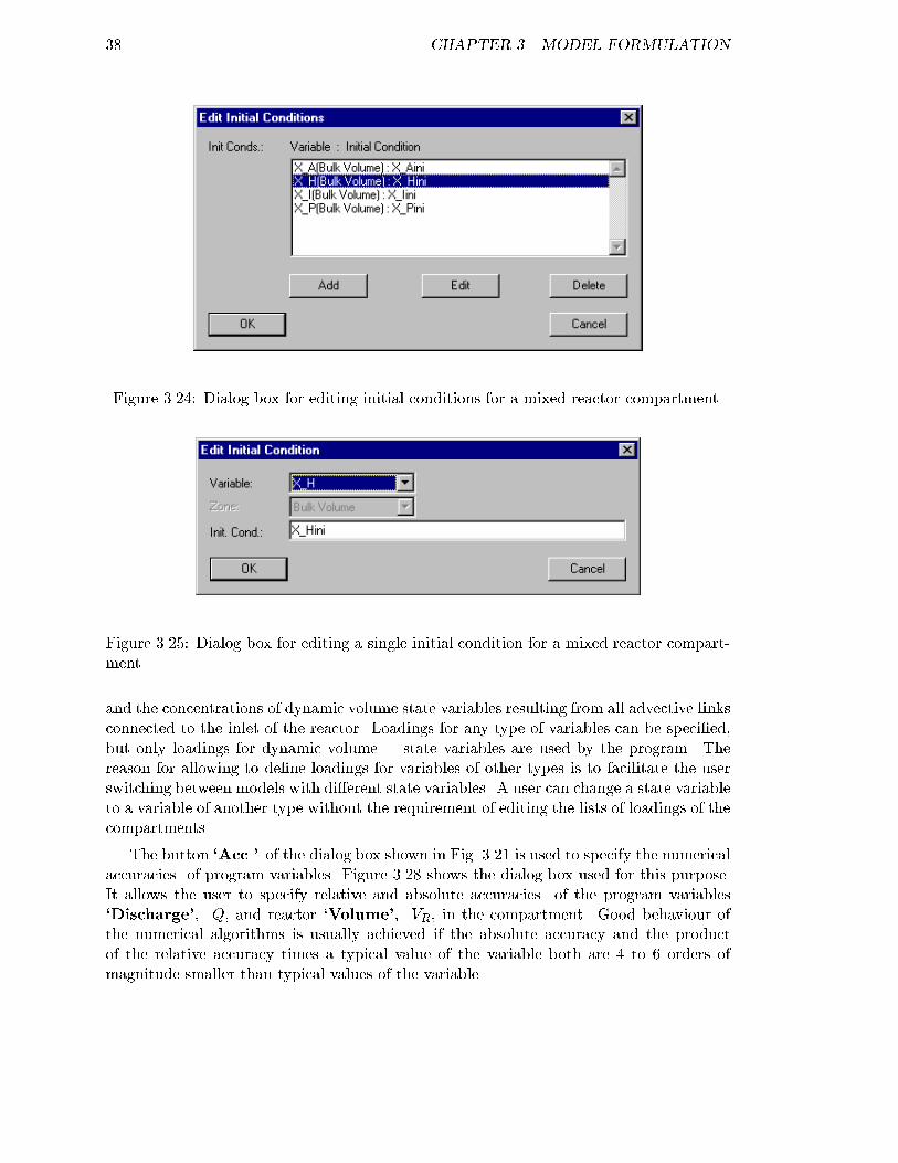
38 CHAPTER 3. MODEL FORMULATION
Figure 3.24: Dialog box for editing initial conditions for a mixed reactor compartment.
Figure 3.25: Dialog box for editing a single initial condition for a mixed reactor compart-
ment.
and the concentrations of dynamic volume state variables resulting from all advective links
connected to the inlet of the reactor. Loadings for any type of variables can be speci�ed,
but only loadings for dynamic volume state variables are used by the program. The
reason for allowing to de�ne loadings for variables of other types is to facilitate the user
switching between models with di�erent state variables. A user can change a state variable
to a variable of another type without the requirement of editing the lists of loadings of the
compartments.
The button `Acc.' of the dialog box shown in Fig. 3.21 is used to specify the numerical
accuracies of program variables. Figure 3.28 shows the dialog box used for this purpose.
It allows the user to specify relative and absolute accuracies of the program variables
`Discharge', Q, and reactor `Volume', VR, in the compartment. Good behaviour of
the numerical algorithms is usually achieved if the absolute accuracy and the product
of the relative accuracy times a typical value of the variable both are 4 to 6 orders of
magnitude smaller than typical values of the variable.

3.3. COMPARTMENTS 39
Figure 3.26: Dialog box for editing inputs to a mixed reactor compartment.
In Table 3.4 the program variables available in a mixed reactor compartment are sum-
marized (for a complete overview of all program variables see Table 3.1 on page 17).
Calculation Number Identi�er for calculations (value set in the dialog boxes shownin Figs. 4.5 and 4.17).
Time Simulation time.
Compartment Index Identi�er for compartments (value set in the dialog box shownin Fig. 3.21).
Zone Index Identi�er for zones within compartments (returns a value of0).
Discharge Volumetric ow rate.
Water Fraction Volumetric fraction of water (returns a value of 1).
Reactor Volume Total volume of the reactor.
Bulk Volume Volume of mixed water zone (returns the value of the reactorvolume).
Table 3.4: Program variables available in the mixed reactor compartment.

40 CHAPTER 3. MODEL FORMULATION
Figure 3.27: Dialog box for editing a single input to a mixed reactor compartment.
Figure 3.28: Dialog box for editing the accuracies of program variables of a mixed reactor
compartment.

3.3. COMPARTMENTS 41
3.3.2 Bio�lm Reactor Compartment
Overview
A bio�lm consists of a solid matrix with pore water that can contain dissolved substances
and suspended solids. The growth or decay of organisms forming the solid matrix
leads to expansion or shrinking of the bio�lm. The consumption of substrate of the
organisms present at a high concentration in the bio�lm solid matrix can lead to a
growth limitation by the di�usive mass transfer into the depth of the bio�lm. The bio�lm
reactor compartment of AQUASIM describes a reactor with a completely mixed bulk
water volume and with a bio�lm growing on a substratum surface in the reactor. Solids
can attach or detach at the surface of the bio�lm and in its interior. Any transformation
processes can be de�ned. The description of the bio�lm in AQUASIM is one-dimensional.
Only the direction perpendicular to the substratum, which has the largest concentration
gradients, is resolved. All variables are averaged over areas parallel to the substratum.
Bio�lm reactor compartments can be linked advectively or di�usively to other AQUASIM
compartments.
Equations Solved by AQUASIM
The equations solved in the bio�lm reactor compartment are based on the development
of a one-dimensional mixed-culture bio�lm model since 1984 (Wanner and Gujer, 1984;
Wanner and Gujer, 1986; Gujer and Wanner, 1990; Wanner, 1994; Wanner, 1995; Wanner
and Reichert, 1996; Reichert and Wanner, 1997). The equations as they are solved by
AQUASIM are described in the last two papers of this list. In the following, a summary
of these equations is given.
In order to formulate the one-dimensional conservation laws
@�
@t+
@ j
@z= r (3.6)
compartment-speci�c expressions for the one-dimensional density, � (amount of conserved
quantity per unit compartment length), for the one-dimensional ux, j (amount of the
conserved quantity transported per unit time), and for the one-dimensional source term,
r (amount produced per unit compartment length and per unit time), must be derived.
Three zones are distinguished in the bio�lm reactor compartment. Variables present
in di�erent zones are distinguished by the index `M' for the solid matrix, `P' for the pore
volume, and `B' for the bulk volume. In addition, the index `F' is used for bio�lm,
when the distinction into solid matrix and pore volume is not relevant (e.g. for the bio�lm
thickness, LF ). The spatial dimension perpendicular to the substratum is resolved by
the space coordinate z. This coordinate takes a value of zero at the substratum and it
increases with increasing distance from the substratum up to the bio�lm thickness, LF .
In order to formulate the bio�lm equations, 4 types of components of a conservation law
must be distinguished: The array of one-dimensional densities of these types of components
is given as follows:
� =
0BB@
AXM;i
AXP;i
A�l;FCP;i
A�
1CCA (3.7)

42 CHAPTER 3. MODEL FORMULATION
The �rst component of equation 3.7 describes particulate species in the bio�lmmatrix. The
one-dimensional density of these species is given as the product of the area parallel to the
substratum, A, and the concentration of particulate species in the bio�lm matrix averaged
over this area, XM;i. The second component of equation 3.7 describes the particulate
species in the bio�lm pore water. Similarly to the �rst component, the one-dimensional
density of these species is given as the product the area parallel to the substratum, A, and
the concentration of these species averaged over this area, XP;i. Note that this implies a
de�nition of a concentration of particulate species as mass per unit of total volume and
not only per unit of pore water volume. This de�nition makes the concentrations XM;i
and XP;i comparable with each other. Note, however, that this leads to a step in the
concentration XP;i at the bio�lm surface, because there is no solid matrix in the bulk
volume and the concentration of suspended solids is continuous if de�ned as mass per
unit of water phase volume. The third component of equation 3.7 describes substances
dissolved in the pore water of the bio�lm. The concentration of dissolved substances is
de�ned as mass per unit of water phase volume. Therefore, their one-dimensional density
is given as the product of the area parallel to the substratum, A, the liquid phase volume
fraction, �l;F , and the concentration of the dissolved species averaged over the area A,
CP;i. All concentrations, Xi and Ci, are represented in AQUASIM as dynamic volume
state variables. The liquid phase volume fraction is given as
�l;F = � �
nXXi=1
XP;i
�Xi
(3.8)
where �Xiis the density of the particulate species described by the concentration Xi, nX
is the number of particulate species, and � is the porosity of the bio�lm given as unity
minus the volume fraction of the solid matrix
� = 1�
nXXi=1
XM;i
�Xi
(3.9)
The last component of equation 3.7 describes the porosity of the bio�lm. The one-
dimensional density for this variable (free volume per unit bio�lm depth) is given as the
product of the porosity, �, and the area parallel to the substratum, A.
The one-dimensional uxes of the substances with one-dimensional densities as de-

3.3. COMPARTMENTS 43
scribed by equation 3.7 are given as follows:
j =
0BBBBBBBBBBBBBBBBBBBBBBBBB@
AuFXM;i �ADM;Xi
@XM;i
@z
�(1� �)AuFXP;i
�� �ADP;Xi
@�XP;i
�
�@z
+A
nXXk=1
DM;Xk
�Xk
@XM;k
@z
XP;i
�+A
nXXk=1
�DP;Xk
�Xk
@�XP;k
�
�@z
XP;i
�
�(1� �l;F )AuFCP;i � �l;FADP;Ci
@CP;i
@z
+�l;F
�A
nXXk=1
DM;Xk
�Xk
@XM;k
@zCP;i +
�l;F
�A
nXXk=1
�DP;Xk
�Xk
@�XP;k
�
�@z
CP;i
�AuF +A
nXXk=1
DM;Xk
�Xk
@XM;k
@z
1CCCCCCCCCCCCCCCCCCCCCCCCCA
(3.10)
In this equation, uF is the advective velocity of the bio�lm matrix given by
uF =1
A
zZ0
1
1� �
nXXk=1
rM;Xk
�Xk
+ r0�
!Adz0 (3.11)
where r0� is the excess growth of porosity de�ned by
r0� = r� ��
1� �
nXXk=1
rM;Xk
�Xk
(3.12)
and r� is the growth rate of free volume between the solid matrix. With this notation,
the porosity of a bio�lm remains constant if r0� = 0, because the same fraction of free
volume is produced as is of solid matrix volume. The �rst component of equation (3.10)
describes the advective and di�usive ow of solids within the bio�lm matrix. The second
component of equation (3.10) describes advection and di�usion of solids suspended in the
pore volume of the bio�lm. The �rst term of this component describes advection with the
water ow produced by growth and decay of organisms in the bio�lm matrix. Because
the organisms consist mainly of water, in a growing bio�lm, the water contained in the
organisms moving outward at the velocity uF in the solid matrix must be compensated by
water owing through the pore water into the bio�lm. The �rst term describes advection
of suspended solids with this water ow. The second term describes di�usion or Brownian
motion of the solids in the pore water. The third and fourth terms of the second component
describe advection with the water ow induced by di�usion of solids in the solid matrix
and in the pore water, respectively. The third component of equation (3.10) describes
advection and di�usion of dissolved substances in the pore volume of the bio�lm. The
terms have the same meaning as those in the second component for suspended solids. The
last component of equation (3.10) represents the ow of free volume in the bio�lm. Free
volume is transported advectively with velocity uF analogously to the solid matrix, but
di�usive transport in the solid matix has a reverse e�ect on free volume.

44 CHAPTER 3. MODEL FORMULATION
The following one-dimensional source terms are required to complete the set of bio�lm
equations.
r =
0BB@
ArM;Xi�Akde;vol;Xi
XM;i +Akat;vol;XiXP;i
ArP;Xi+Akde;vol;Xi
XM;i �Akat;vol;XiXP;i
ArCiAr�
1CCA (3.13)
In these equations r are transformation rates and kde;vol;Xiand kat;vol;Xi
are substance-
dependent volume detachment and attachment coe�cients, respectively. The terms
containing the detachment and attachment coe�cients describe exchange of solids between
the pore water and the solid matrix of the bio�lm.
Application of the general expression for di�erential conservation laws (3.6) to the
de�nitions given by the equations (3.7) to (3.13) leads to the following set of 4 di�erential
equations.
The �rst equation describes the behaviour of the constituents of the bio�lm solid
matrix:
@XM;i
@t=� uF
@XM;i
@z+
1
A
@
@z
�ADM;Xi
@XM;i
@z
�� r0�XM;i
+
rM;Xi
�XM;i
1� �
nXXk=1
rM;Xk
�Xk
!� kde;volXM;i + kat;volXP;i
(3.14)
The second equation describes the behaviour of solids suspended in the pore water of
the bio�lm:
@XP;i
@t=(1� �)uF
@�XP;i
�
�@z
� uF@�
@z
XP;i
�+
nXXk=1
rM;Xk
�Xk
XP;i
�
+ (1� �)XP;i
�r0� +
1
A
@
@z
0@�ADP;Xi
@�XP;i
�
�@z
1A
�1
A
@
@z
A
nXXk=1
DM;Xk
�Xk
@XM;k
@z
XP;i
�
!
�1
A
@
@z
0@A nXX
k=1
�DP;Xk
�Xk
@�XP;k
�
�@z
XP;i
�
1A
+ rP;Xi+ kde;vol;Xi
XM;i � kat;vol;XiXP;i
(3.15)
The third equation describes the behaviour of substances dissolved in the pore water

3.3. COMPARTMENTS 45
of the bio�lm:
@�l;F
@tCP;i + �l;F
@CP;i
@t=(1� �l;F )uF
@CP;i
@z+
nXXk=1
rM;Xk
�Xk
�l;F
�CP;i
+ (1� �)�l;F
�r0thetaCP;i +
1
A
@
@z
��l;FADP;Ci
@CP;i
@z
�@CP;i
@z
�1
A
@
@z
�l;F
�A
nXXk=1
DM;Xk
�Xk
@XM;k
@zCP;i
!
�1
A
@
@z
0@�l;FA nXX
k=1
DP;Xk
�Xk
@�XP;k
�
�@z
CP;i
1A+ rCi
(3.16)
The fourth equation describes the changes in bio�lm porosity:
@�
@t= �uF
@�
@z�
1
A
@
@z
A
nXXk=1
DM;Xk
�Xk
@XM;k
@z
!+ (1� �)r0� (3.17)
In equation (3.16) @�l;F=@t can be calculated with the aid of the temporal derivative
of equation (3.8):
@�l;F
@t=
@�
@t�
nXXi=1
1
�Xi
@XP;i
@t(3.18)
The above equations must be combined with the equation
dLF
dt= uL (3.19)
describing the temporal change of the bio�lm thickness, LF . In this equation, uL is the
velocity of the interface layer between bio�lm and bulk volume. The velocity uL is given
by
uL = uF (LF )� ude + uat (3.20)
where ude and uat are the detachment and the attachment velocities of solids at the
bio�lm surface, respectively. The detachment velocity, ude, can either be given globally
as a function of the bio�lm thickness, LF , the advective velocity at the bio�lm surface,
uF (LF ), time, t, surface shear stress, �surf , etc.
ude = ude(LF ; uF (LF ); t; �surf ; :::) (3.21a)
or, in the case of a di�usive bio�lm matrix (all DM;Xi> 0), individual surface detach-
ment rate coe�cients, kde;surf;Xi, can be given alternatively. The latter case results in a
detachment velocity of
ude =1
1� �(LF )
nXXk=1
kde;surf;XkXM;k
�Xk
(3.21b)

46 CHAPTER 3. MODEL FORMULATION
The attachment velocity is calculated similarly to the equation (3.21b) as
uat =1
1� �(LF )
nXXk=1
kat;surf;XkXL;k
�Xk
(3.22)
where kat;surf;Xiis the surface attachment coe�cient for the solids described by the
concentrations Xi. In all the above equations, XL;i is the concentration of solids of type i
in the liquid boundary layer above the bio�lm immediately adjacent to the bio�lm surface.
In order to make the solution of the above system of di�erential equations unique,
boundary conditions must be speci�ed.
For the case of a rigid bio�lmmatrix (allDM;Xi= 0) no boundary condition is required
for equation (3.14) at the substratum-bio�lm interface. For the case of a di�usive bio�lm
matrix (all DM;Xi> 0) equation (3.14) is solved with the following boundary condition
at the substratum-bio�lm interface:
@XM;i
@z(z = 0) = 0 (3.23a)
The boundary condition for equation (3.14) at the bio�lm surface is determined by attach-
ment and detachment processes. For a rigid bio�lm matrix (all DM;Xi= 0) the boundary
condition is given by
(uF � uL)XM;i(LF ) =
8<:
(ude � uat)XM;i(LF ) for ude > uat
(ude � uat)kat;surf;Xi
uatXL;i for ude < uat
(3.23b)
For a di�usive bio�lm matrix the boundary condition for equation (3.14) at the bio�lm
surface is given by
(uF � uL)XM;i(LF )�DM;Xi
@XM;i
@z(LF )
= kde;surf;XiXM;i(LF ) � kat;surf;Xi
XL;i (3.23c)
The boundary conditions for equation (3.15) that describes the behaviour of suspended
solids in the bio�lm pore water are given by a no ux condition at the substratum-bio�lm
interface:
@XP;i
@z(z = 0) = 0 (3.24a)
and by a continuity equation of the concentrations in the water at the bio�lm surface
XP;i(LF ) = �(LF )XL;i (3.24b)
Note that due to the de�nition of XP;i as mass per total of bio�lm volume (including the
solid matrix), this continuity condition for concentrations in the water phase leads to a
discontinuity of the values of XP;i at the bio�lm surface. The advantage of the de�nition
of XP;i as mass per unit of total bio�lm volume is that the concentrations XP;i can directly
be compared with the concentrations XM;i of solids in the bio�lm matrix.

3.3. COMPARTMENTS 47
The boundary conditions of equation (3.16) that describes the behaviour of substances
dissolved in the pore water of the bio�lm are as follows. At the substratum-bio�lm in-
terface, the boundary condition is given as a continuity equation of the ow through the
substratum
�A�l;FDP;Ci
@CP;i
@z(z = 0) = Isubstr;Ci (3.25a)
The total ow through the substratum, Isubstr;Ci , is zero (impermeable substratum) unless
a di�usive link is connected to the bottom of the bio�lm in order to model a permeable
membrane. In the latter case the ow through the substratum is proportional to the
di�erence between the substance concentration in the pore water and the concentration in
the other compartment connected to the di�usive link (the substance-speci�c constants of
proportionality are de�ned in the link de�nition). The boundary condition at the bio�lm
surface is a continuity condition for the concentration in the water
CP;i(LF ) = CL;i (3.25b)
The equation (3.17) does not require any boundary conditions.
The total ows of solids out of the bio�lm (negative values for ows into the bio�lm)
are given as
IL;Xi=AuFXM;i �ADF;Xi
@XM;i
@z(LF )
� (1� �)AuFXP;i
�� �ADP;Xi
@�XP;i
�
�@z
(LF )
+A
nXXk=1
DM;Xk
�Xk
@XM;k
@z
XP;i
�(LF ) +A
nXXk=1
�DP;Xk
�Xk
@�XP;k
�
�@z
XP;i
�(LF )
�AuLXM;i(LF )
(3.26)
This expression is the sum of the ow from the solid matrix and the pore volume at z = LFplus the last term correcting for the movement of the bio�lm surface.
The total ows of dissolved substances out of the bio�lm (negative values for ows into
the bio�lm) are given as
IL;Ci =� (1� �)�l;F
�AuFCP;i(LF )� �l;FADP;Ci
@CP;i
@z(LF )
+�l;F
�A
nXXk=1
DM;Xk
�Xk
@XM;k
@z
XP;i
�(LF )
+�l;F
�A
nXXk=1
�DP;Xk
�Xk
@�XP;k
�
�@z
XP;i
�(LF )
�AuL�l;FCP;i(LF )
(3.27)
This expression is the ow at z = LF plus a correction that considers the movement of
the interface.
The equations for the bio�lm described so far are connected to the bulk volume of the
bio�lm reactor through a liquid boundary layer. In AQUASIM the liquid boundary layer

48 CHAPTER 3. MODEL FORMULATION
is only roughly described with the aid of a mass transfer resistance (Wanner and Reichert,
1996). The equation for particulate components is given as
XL;i �XB;i =�L;Xi
A(LF )IL;Xi
(3.28)
A similar expression describes the behaviour of the dissolved components
CL;i � CB;i =�L;CiA(LF )
IL;Ci (3.29)
In these equations, �L;Xiand �L;Ci are the di�usive resistances for the substances Xi
and Ci, and XB;i and CB;i are the concentrations in the bulk volume. Note that for the
case of a resistance of zero, a continuity equation for the concentrations in the liquid layer
adjacent to the bio�lm and in the bulk volume results.
As a last series of equations, the equations for the bulk volume must be given.
The mass balance for particulate substances in the bulk volume is given as
d
dt(VBXB;i) = Iin;Xi
�XB;iQef + IL;Xi+ VBrXi
(3.30)
where VB is the bulk volume, Iin;Xiis the total input of the substance described by
the concentration Xi into the bulk volume through advective and di�usive links and as
speci�ed as input in the compartment de�nition.
The mass balance equation for dissolved substances in the bulk volume is given as
d
dt(VB�l;BCB;i) = Iin;Ci � �l;BCB;iQef + IL;Ci + VBrCi (3.31)
where �l;B is the liquid phase volume fraction in the bulk volume (the porosity is equal
to unity in the bulk volume).
In AQUASIM, two types of reactors are distinguished: A con�ned rreactor has a
constant total reactor volume for the bio�lm and the bulk water. For this reactor type
the bulk volume is calculated as
VB = VR �
LFZ0
A(z0)dz0 ; VR = const (3.32a)
where VR is the constant total reactor volume. The uncon�ned reactor type describes
a reactor with a constant bulk volume. For this reactor type, the total reactor volume,
VR, is not constant but is given as the sum of the (variable) bio�lm volume and the bulk
volume as
VR =
LFZ0
A(z0)dz0 + VB ; VB = const (3.32b)
The e�uent discharge, Qef , depends on the in uent and on the varying reactor volume.
In the case of the con�ned rector
Qef = Qin (3.33a)
whereas due to the varying total volume for the uncon�ned reactor
Qef = Qin �AuL (3.33b)

3.3. COMPARTMENTS 49
User De�nitions
Within a bio�lm reactor compartment three zones, the Bulk Volume, the Biofilm Matrix
and the Pore Water are distinguished. Variables and process rates can be made dependent
on the zone by using the program variable Zone Index which takes the value 0 in the
bulk volume zone, 1 in the bio�lm matrix zone and 2 in the pore water zone.
Figure 3.29 shows the dialog box used for de�ning or editing a bio�lm reactor com-
partment. The edit �eld `Name' is used to specify the name of the compartment. Each
Figure 3.29: Dialog box for editing a bio�lm reactor compartment.
compartment needs a unique name as an identi�er. A name of a compartment consists of a
sequence of letters (A-Z,a-z), digits (0-9) and underline characters ( ). The �rst character
may not be a digit.
The edit �eld `Comp. Index' can be used to specify a nonnegative integer number
as a compartment index. This value can be accessed with the aid of the program variable
Compartment Index to make variables or process rates dependent on the compartment.
To improve documentation of compartments, the edit �eld `Description' can option-
ally be used to store comments on speci�c implementation features of a compartment.
The buttons `Variables', `Processes', `Init. Cond.' and `Input' are used to
activate and inactivate state variables, to activate and inactivate processes, to specify
initial conditions and to de�ne inputs to a compartment, respectively. These options are
described later in this subsection.
The buttons `Particulate Variables' and `Dissolved Variables' are used to de�ne
properties of dissolved or particulate substances for dynamic volume state variables.
These options are also described later in this subsection.

50 CHAPTER 3. MODEL FORMULATION
The next option allows the user to select the reactor type. Selection of the radio
button `con�ned' leads to the use of a reactor with a constant total volume for bio�lm
and bulk uid. The value for this total reactor volume can be speci�ed in the edit �eld
labelled `Reactor Vol.'. In such a reactor, growth of the bio�lm leads to a decrease in
bulk volume as described by equation (3.32a). Selection of the radio button `uncon�ned'
leads to the use of a reactor with a constant bulk volume. In this case, a growing bio�lm
leads to a growth in total reactor volume. The value of the bulk volume can be speci�ed
in the edit �eld `Bulk Volume'. This option can be used to model free-surface water
ow over a bio�lm.
The next option is used to select the properties of the pore volume. Selection of the
radio button `liquid phase only' leads to a model without suspended solids in the pore
water. Such a model is adequate to describe a dense bio�lm with very small pores in
which there is no relevant motion of suspended solids. Selection of the radio button `with
suspended solids' leads to a model in which solids can penetrate a bio�lm within the
pore water. Such a model is suitable to describe bio�lms with a high porosity.
The radio buttons `rigid' and `di�usive' allow the user to select how the bio�lm
matrix should be modelled. In a rigid bio�lm matrix there is no di�usive mass transport
of solids, whereas in a di�usive bio�lm matrix a small e�ective di�usion is also allowed for
solids in the bio�lm matrix. This option requires the di�usivities DM;Xito be speci�ed as
properties of particulate variables as described later in this subsection.
The treatment of surface detachment of solids from the bio�lm can be selected with the
aid of the radio buttons `individual rate' and `global velocity' If individual rate is
selected, detachment is calculated with the aid of the substance-speci�c detachment rate
coe�cient, kde;surf;Xi. This option can only be selected for a di�usive bio�lm matrix. If
this option is selected, the detachment velocity, ude is calculated according to the equation
(3.21b). If a global detachment velocity, ude, is speci�ed, solids are detached from the
bio�lm according to their relative occurrence at the bio�lm surface.
The edit �eld `Bio�lm Area' is used to specify the area of the bio�lm, A, as a function
of the distance from the substratum, z, which is accessible by the program variable Space
Coordinate Z. It is not allowed to use a time dependence or a dependence on state
variables for the speci�cation of the bio�lm area. Some possibilities for this function are:
A constant surface area
A = const (3.34a)
describes a planar bio�lm, a surface area of the form
A = 2�Lcy(rcy + z) (3.34b)
describes a bio�lm growing on the outside of a cylinder with radius rcy and length Lcy, a
surface area of the form
A = 2�Lcy(rcy � z) (3.34c)
describes a bio�lm growing on the inside of a cylinder with radius rcy and length Lcy, and
a surface area of the form
A = 4�nsp(rsp + z)2 (3.34d)
describes bio�lms growing on nsp spherical particles of radius rsp.

3.3. COMPARTMENTS 51
The edit �eld `Rate Porosity' is used to specify the excess growth rate of porosity,
r0�, de�ned in equation (3.12). If this rate is set to zero and if no volume attachment or
detachment is active, the porosity of the bio�lm remains constant.
As last options, `Num. Grid Pts.', `Resolution' and `Acc.', in the dialog box
used for the de�nition of a bio�lm reactor compartment (Fig. 3.29) the user can select
the number of grid points, the discretization order of the numerical algorithm and the
accuracies of program variables. The number of grid points is used to specify by how
many discrete points the continuous z-axis is approximated. If the number of grid points
is set to ngp, the depth of the bio�lm is resolved into 2 boundary points and ngp � 2
grid points located in the middle of ngp � 2 cells of equal thickness. Two additional grid
points are used to describe the boundary layer and the bulk volume. For the division
of the z-axis described above the `low resolution' method applies a simple �rst-order
discretization scheme that is very robust but can have signi�cant numerical di�usion. The
`high resolution' method uses a second-order discretization scheme that applies ux-
limiters to avoid oscillations of the numerical solutions (Reichert, 1994b, chapter 6). The
high resolution method is not yet implemented in the bio�lm compartment of the current
version of AQUASIM. The button `Acc.' is used to specify the numerical accuracies of
program variables as described later in this subsection.
The check box `active for calculation' can be used to activate or inactivate the
compartment from the calculations. This check box has the same functionality as the
buttons Activate and Inactivate in the dialog box shown in Fig. 3.19.
As for each compartment, the user has to select which state variables are active. This
is done by clicking the button `Variables' of the dialog box shown in Fig. 3.29. This action
opens the dialog box shown in Fig. 3.30. The two list boxes of this dialog box show the
Figure 3.30: Dialog box for activating and inactivating state variables in a compartment.
active variables and the available variables, respectively. The button `Activate' is used
to activate available variables selected in the right list box, and the button `Inactivate'
is used to inactivate active variables selected in the left list box. If an active variable is
selected while activating another variable, the new active variable is inserted in the list of
active variables immediately before the selected variable, otherwise it is appended to the

52 CHAPTER 3. MODEL FORMULATION
end of the list of active variables. This gives the user the possibility to in uence the order
of active variables (the order is irrelevant for the program, but it may be convenient for
the user to have a certain order). The list of active variables may contain variables of any
type, but activation has only an e�ect to state variables. Inactive state variables return
a value of zero. The reason for allowing other types of variables in the list of active state
variables is to facilitate switching between di�erent models that do not contain the same
state variables. A user can change a state variable to a variable of another type without
the requirement of editing the lists of active variables of the compartments.
Similarly to the activation of state variables, the user has to select which processes are
active in a compartment. This is done by clicking the button `Processes' of the dialog
box shown in Fig. 3.29. This action opens the dialog box shown in Fig. 3.31. The two list
Figure 3.31: Dialog box for activating and inactivating processes in a compartment.
boxes in this dialog box show the active processes and the available processes, respectively.
The button `Activate' is used to activate available processes selected in the right list box,
and the button `Inactivate' is used to inactivate an active processes selected in the left
list box. If an active process is selected while activating another process, the new active
process is inserted in the list of active processes immediately before the selected process,
otherwise it is appended to the end of the list of active processes. This gives the user
the possibility to in uence the order of active processes (the order is irrelevant for the
program, but it may be convenient for the user to have a certain order).
Initial conditions for a bio�lm reactor compartment can be speci�ed by clicking the
button `Init. Cond.' of the dialog box shown in Fig. 3.29. This action opens the dialog
box shown in Fig. 3.32. This dialog box shows a list of all initial conditions already
speci�ed. Each row of the list box contains the name of a variable, followed by the zone
of the compartment for which the initial condition is speci�ed (in brackets) and by the
algebraic expression specifying the initial value. For each combination of a variable with
a zone only one unique initial condition can be speci�ed. The list of initial conditions
can be edited using the buttons `Add', `Edit' and `Delete'. If an initial condition is
selected while adding a new initial condition, the new initial condition is inserted in the
list immediately before the selected initial condition, otherwise it is appended to the end

3.3. COMPARTMENTS 53
Figure 3.32: Dialog box for editing initial conditions for a bio�lm reactor compartment.
of the list of initial conditions. This gives the user the possibility to in uence the order
of the initial conditions (the order is irrelevant for the program, but it may be convenient
for the user to have a certain order). The dialog box used for editing a single initial
condition is shown in Fig. 3.33. In this dialog box the �elds `Variable', `Zone' and `Init.
Figure 3.33: Dialog box for editing a single initial condition for a bio�lm reactor compart-
ment.
Cond.' allow the user to select a variable and a zone and to specify an initial condition.
In a bio�lm compartment there are the zones Bulk Volume, Biofilm Matrix and Pore
Volume. Initial conditions for any type of variables can be speci�ed, but only initial
conditions for state variables and for the program variable Biofilm Thickness are used
by the program. The reason for allowing to de�ne initial conditions for variables of other
types is to facilitate the users switching between models with di�erent state variables. A
user can change a state variable to a variable of another type without the requirement of
editing the lists of initial conditions of the compartments. Initial conditions of a bio�lm
reactor compartment may not depend on state variables and they can only depend on
the program variables Calculation Number, Time and Space Coordinate Z.
Input to a bio�lm reactor compartment can be speci�ed by clicking the button `Input'
of the dialog box shown in Fig. 3.29. This action opens the dialog box shown in Fig. 3.34.

54 CHAPTER 3. MODEL FORMULATION
The edit �eld `Water In ow' of this dialog box is used to specify the discharge of water
Figure 3.34: Dialog box for editing inputs to a bio�lm reactor compartment.
into the bulk volume of the reactor, Qin, and the list box contains substance loadings,
Iin;Ci and Iin;Xi, into the bulk volume. For each variable only one unique loading can
be speci�ed. The list of loadings can be edited using the buttons `Add', `Edit' and
`Delete'. If a loading is selected while adding a new loading, the new loading is inserted
in the list immediately before the selected loading, otherwise it is appended to the end of
the list of loadings. This gives the user the possibility to in uence the order of the loadings
(the order is irrelevant for the program, but it may be convenient for the user to have a
certain order). Figure 3.35 shows the dialog box used to specify a single input loading of a
substance. In this dialog box the �elds `Variable' and `Loading' allow the user to select
Figure 3.35: Dialog box for editing a single input loading to a bio�lm reactor compartment.
a variable and to specify a loading, Iin;Ci or Iin;Xi. Note that this loading represents a
mass per unit of time. A loading to a bio�lm reactor compartment may depend on the
program variables Discharge and on dynamic volume state variables. These variables
return the discharge and the concentrations of dynamic volume state variables resulting
from all advective links connected to the inlet of the reactor. Loadings for any type of
variables can be speci�ed, but only loadings for dynamic volume state variables are used
by the program. The reason for allowing to de�ne loadings for variables of other types is

3.3. COMPARTMENTS 55
to facilitate the user switching between models with di�erent state variables. A user can
change a state variable to a variable of another type without the requirement of editing
the lists of input loadings of the compartments.
The button `Particulate Variables' of the dialog box shown in Fig. 3.29 allows the
user to specify properties of particulate variables. Figure 3.36 shows the dialog box used
for this purpose. It contains a list box with the names of all de�ned particulate variables.
Figure 3.36: Dialog box for editing properties of particulate variables in a bio�lm reactor
compartment.
Note that a variable can only be in one of the lists of particluate and dissolved variables.
The buttons `Add', `Edit' and `Delete' allow the user to edit this list. Figure 3.37
shows the dialog box used to specify the properties of a particulate variable in a bio�lm
reactor compartment. The �eld `Variable' allows the user to select a variable for which
Figure 3.37: Dialog box for editing properties of a single particulate variable in a bio�lm
reactor compartment.

56 CHAPTER 3. MODEL FORMULATION
particulate properties are to be de�ned. The edit �eld `Density' is used to specify the
density, �Xi, of the variable. The expression for the density may not depend on time. The
edit �elds `Surf. Att. Coe�.', `Surf. Det. Coe�.', `Vol. Att. Coe�.' and `Vol.
Det. Coe�.' are used to specify expressions for the surface and volume attachment
and detachment coe�cients, kat;surf , kde;surf , kat;vol and kde;vol, respectively. Note that
the values entered for the surface detachment coe�cient only has an e�ect if the radio
button individual rate of the option Surf. Detach. of the dialog box shown in Fig.
3.29 is selected. Similarly the expressions entered for volume attachment and detachment
coe�cients are only used if the radio button with free particles is selected for the
option Pore Volume of the dialog box shown in Fig. 3.29. The edit �eld `Bound. L.
Res.' is used to specify the boundary layer resistance, �L;Xi, for the particulate species
described by the concentration Xi. The last two edit �elds, `Pore Di�.' and `Matrix
Di�.' are used to specify the coe�cients for pore volume di�usion, DP;Xiand DM;Xi
,
respectively. Note that the �rst of these values has only an e�ect if the radio button with
free particles is selected for the option `Pore Volume' of the dialog box shown in Fig.
3.29 and that the second value only has an e�ect if the radio button diffusive for the
option Biofilm Matrix is selected. Otherwise the values entered here are ignored.
The button `Dissolved Variables' of the dialog box shown in Fig. 3.29 allows the
user to specify properties of dissolved variables. Figure 3.38 shows the dialog box used for
this purpose. It contains a list box with the names of all de�ned dissolved variables. Note
Figure 3.38: Dialog box for editing properties of dissolved variables in a bio�lm reactor
compartment.
that a variable can only be in one of the lists of particluate and dissolved variables. The
buttons `Add', `Edit' and `Delete' allow the user to edit this list. Figure 3.39 shows
the dialog box used to specify the properties of a dissolved variable in a bio�lm reactor
compartment. The �eld `Variable' allows the user to select a variable for which dissolved
properties are to be de�ned. The edit �eld `Bound. L. Res.' is used to specify the
boundary layer resistance, �L;Ci , for the dissolved species described by the concentration
Ci. The last edit �eld, `Pore Di�.' is used to specify the coe�cient for pore volume
di�usion, DP;Ci of the dissolved species described by the concentration Ci.
The button `Acc.' of the dialog box shown in Fig. 3.29 is used to specify the numerical
accuracies of program variables. Fig. 3.40 shows the dialog box used for this purpose.

3.3. COMPARTMENTS 57
Figure 3.39: Dialog box for editing properties of a single dissolved variable in a bio�lm
reactor compartment.
It allows the user to specify relative and absolute accuracies of the program variables
`Discharge', Q, reactor or bulk `Volume', VR or VB , `Bio�lm Thickness', LF , and
`Water Fraction', �l;F (the last value is also used as the accuracy of the volume fractions
of particulate species in the bio�lm). Good behaviour of the numerical algorithmsis usually
achieved if the absolute accuracy and the product of the relative accuracy times a typical
value of the variable both are 4 to 6 orders of magnitude smaller than typical values of
the variable.
In Table 3.5 the program variables available in a bio�lm reactor compartment are sum-
marized (for a complete overview of all program variables see Table 3.1 on page 17).

58 CHAPTER 3. MODEL FORMULATION
Figure 3.40: Dialog box for editing the accuracies of program variables of a bio�lm reactor
compartment.
Calculation Number Identi�er for calculations (value set in the dialog box shownin Figs. 4.5 and 4.17).
Time Simulation time.
Compartment Index Identi�er for compartments (value set in the dialog box shownin Fig. 3.29).
Zone Index Identi�er for zones within compartments (returns a value of0 in the bulk volume zone, a value of 1 in the bio�lm matrix,and a value of 2 in the bio�lm pore volume).
Discharge Volumetric ow rate.
Water Fraction Volumetric fraction of water.
Space Coordinate Z Depth coordinate in the bio�lm (zero at the substratum-bio�lm interface).
Reactor Volume Total volume of the reactor.
Bulk Volume Volume of mixed water zone outside of the bio�lm.
Biofilm Thickness Thickness of the bio�lm.
Growth Velocity of Biofilm Advective velocity of bio�lm solid matrix.
Interface Velocity of Biofilm Velocity of the interface between bio�lm and bulk uid.
Detachment Velocity of Biofilm Detachment velocity of particles from the bio�lm surface.
Attachment Velocity of Biofilm Attachment velocity of particles onto the bio�lm surface.
Table 3.5: Program variables available in the bio�lm reactor compartment.

3.3. COMPARTMENTS 59
3.3.3 Advective-Di�usive Reactor Compartment
Overview
The advective-di�usive reactor compartment of AQUASIM can be used to describe one-
dimensional advective-di�usive transport of substances in a ow-through reactor, exchange
with settled, sorbed or sessile substances or organisms, and substance transformations.
The inlet and outlet of the advective-di�usive reactor compartment can be linked advec-
tively to other AQUASIM compartments.
Equations Solved by AQUASIM
In order to formulate the one-dimensional conservation laws
@�
@t+
@ j
@x= r (3.35)
compartment-speci�c expressions for the one-dimensional density, � (amount of conserved
quantity per unit compartment length), for the one-dimensional ux, j (amount of the
conserved quantity transported per unit time), and for the one-dimensional source term,
r (amount produced per unit compartment length and per unit time), must be derived.
For the case of the advective-di�usive reactor compartment, 3 types of components of
a conservation law must be distinguished. The array of one-dimensional densities of these
types of components is given as follows:
� =
0@ A
ACi
Si
1A (3.36)
The �rst component of equation (3.36) describes the conservation of water volume within
the compartment (water is approximated to be incompressible). The one-dimensional
density of water volume in the compartment (volume per unit length) is given by the
cross-sectional area, A, of the compartment. The second component of equation (3.36)
describes substances transported dissolved or suspended with the water ow. Their one-
dimensional densities are given as the product of the cross-sectional area, rA, and the
laterally averaged concentration, Ci. The last component of equation (3.36) describes
substances settled to the bottom or sorbed to surfaces within the compartment.
The value of the variable A must be speci�ed as a function of the distance along the
compartment, x. Its current value is then generally accessible by the program variable
Cross Sectional Area. The variables Ci are represented by dynamic volume state vari-
ables, and the variables Si are represented by dynamic surface state variables. For
equilibrium state variables algebraic equations speci�ed as equilibrium processes are
solved everywhere along the compartment.
The one-dimensional uxes of the quantities with one-dimensional densities as de-
scribed by equation (3.36) are given as follows:
j =
0BB@
Q
QCi �AD@Ci
@x0
1CCA (3.37)

60 CHAPTER 3. MODEL FORMULATION
In this equation Q refers to the volumetric discharge through the compartment, and D
is the coe�cient of longitudinal di�usion or dispersion.
The following one-dimensional source terms are required to complete the set of equa-
tions for the advective-di�usive reactor compartment:
r =
0B@
q
ArCi +�1+sign(q)
2
�qClat;i +
�1�sign(q)
2
�qCi
rSi
1CA (3.38)
The �rst component of equation (3.38) describes the lateral water in ow as volume per
unit length of the compartment, q. In many cases, this longitudinal in ow is zero and the
only in ow is that at the compartment inlet. This in ow is speci�ed as a boundary condi-
tion below (3.42a). The second component describes the e�ect of transformation processes
in the compartment and the e�ect of lateral in ows or out ows (Clat;i is the concentra-
tion in the lateral in ow q). The last component describes the e�ect of transformation
processes on settled of sorbed substances or of growing organisms.
Application of the general law for di�erential conservation laws (3.35) to the de�nitions
given by the equations (3.36) to (3.38) leads to the following set of 3 di�erential equations.
The �rst equation describes water ow through the compartment:
@Q
@x= q (3.39)
The spatial gradient of the discharge, Q, is determined by the lateral in ow, q. Positive
values of q (in ow) increase the downstream discharge, negative values (out ow) decrease
the downstream discharge.
The second equation describes the behaviour of substances transported in the com-
partment:
@Ci
@t= �
1
A
@
@x
�QCi
�+
1
A
@
@x
�AD
@Ci
@x
�+ rCi
+�1+sign(q)
2
� qACin;i +
�1�sign(q)
2
� qACi (3.40)
The concentration is a�ected by advection with the water ow (�rst term), dispersion or
di�usion (second term), transformation processes (third term) and by lateral in ow or
out ow (fourth and �fth terms).
The third equation describes the behaviour of settled or sorbed substances or of sessile
organisms:
@Si
@t= rSi (3.41)
The concentration of such substances is only a�ected by transformation processes. Note
that settling or sorption must also be formulated as a transformation process transforming
dissolved species, Ci, to settled or sorbed species, Si.
In order to make the solution to the above system of di�erential equations unique,
one boundary condition for the ordinary di�erential equation (3.39) and two boundary
conditions for the partial di�erential equation (3.40) are required. The ordinary di�eren-
tial equation (3.41) that does not contain spatial derivatives does not require boundary
conditions.

3.3. COMPARTMENTS 61
The boundary condition for equation (3.39) that describes discharge through the com-
partment is given by
Q(xs) = Qin (3.42a)
at the start point, xs, of the column. According to equation (3.39), due to the lateral
in ow, q, this results in a discharge of
Q(xe) = Q(xs) +
xeZxs
q dx (3.42b)
at the end of the compartment.
The boundary conditions for equation (3.40) are given by the continuity of the sub-
stance loadings entering the compartment and by a `transmission boundary condition'
(Shamir and Harleman, 1967) at the end of the compartment:
QCi(xs)�AD@Ci
@x(xs) = Iin;Ci (3.43a)
@2Ci
@x2= 0 (3.43b)
where Iin;Ci is the total (given) mass input of the substance described by the concentration
Ci per unit of time. The second of these boundary conditions (3.43b) is omitted for
dispersion-free transport.
User De�nitions
Figure 3.41 shows the dialog box used for de�ning or editing an advective-di�usive reactor
compartment. The edit �eld `Name' is used to specify the name of the compartment.
Figure 3.41: Dialog box for editing an advective-di�usive reactor compartment.

62 CHAPTER 3. MODEL FORMULATION
Each compartment needs a unique name as an identi�er. A name of a compartment
consists of a sequence of letters (A-Z,a-z), digits (0-9) and underline characters ( ). The
�rst character may not be a digit.
The edit �eld `Comp. Index' can be used to specify a nonnegative inter number as
a compartment index. This value can be accessed with the aid of the program variable
Compartment Index to make variables or process rates dependent on the compartment.
To improve documentation of compartments, the edit �eld `Description' can option-
ally be used to store comments on speci�c implementation features of a compartment.
The buttons `Variables', `Processes', `Init. Cond.' and `Input' are used to
activate and inactivate state variables, to activate and inactivate processes, to specify
initial conditions and to de�ne inputs to a compartment. These options are described
later in this subsection.
The edit �elds `Start Coord.' and `End Coord.' are used to de�ne the location
of the compartment inlet, xs, and of the compartment outlet, xe, respectively. The values
of variables are resolved continuously with the space coordinate x between these two
locations. Although all equations in this subsection are formulated with the x-axis pointing
in ow direction (xs < xe), the program works also correctly with an x-axis de�ned in the
reverse direction (xs > xe).
The edit �eld `Cross Sect.' is used to specify the wetted cross-sectional area of the
compartment, A, as a function of the longitudinal spatial coordinate x, which is accessible
by the program variable Space Coordinate X. Note that when the advective-di�usive
reactor compartment is used to model a porous medium, A is given as the product of the
porosity and the total cross-sectional area. It is not allowed to use a time dependence or
a dependence on state variables for the speci�ction of the cross-sectional area.
As a next option, `Di�usion', in the dialog box shown in Fig. 3.41 the user can
select how to model di�usion or dispersion. If the user selects the radio button `without
di�usion', a purely advective equation with D = 0 is solved (note, however, that due
to the spatial discretization numerical di�usion can occur). If the user selects the radio
button `with di�usion' a positive di�usion or dispersion coe�cient D must be speci�ed.
This coe�cient can be made dependent on time, discharge or cross-sectional area by using
the program variables Time, Discharge or Cross-Sectional Area.
As last options, `Num. Grid Pts.', `Resolution' and `Acc.', in the dialog box used
for the de�nition of an advective-di�usive reactor compartment (Fig. 3.41) the user can
select the number of grid points, the discretization order of the numerical algorithm and
the accuracies of program variables. The number of grid points is used to specify by how
many discrete points the continuous x-axis is approximated. If the number of grid points
is set to ngp, the compartment is resolved longitudinally into 2 boundary points and ngp�2
grid points located in the middle of ngp�2 cells of equal thickness. For this division of the
x-axis the `low resolution' method applies a simple �rst-order discretization scheme that
is very robust but can have signi�cant numerical di�usion. The `high resolution' method
uses a second-order discretization scheme that applies ux-limiters to avoid oscillations of
the numerical solutions (Reichert, 1994b, chapter 6). The button `Acc.' is used to specify
the numerical accuracies of program variables as described later in this subsection.
The check box `active for calculation' can be used to activate or inactivate the
compartment from the calculations. This check box has the same functionality as the
buttons Activate and Inactivate in the dialog box shown in Fig. 3.19.
As for each compartment, the user has to select which state variables are active. This
is done by clicking the button `Variables' of the dialog box shown in Fig. 3.41. This action

3.3. COMPARTMENTS 63
opens the dialog box shown in Fig. 3.42. The two list boxes of this dialog box show the
Figure 3.42: Dialog box for activating and inactivating state variables in a compartment.
active variables and the available variables, respectively. The button `Activate' is used
to activate available variables selected in the right list box, and the button `Inactivate'
is used to inactivate active variables selected in the left list box. If an active variable is
selected while activating another variable, the new active variable is inserted in the list of
active variables immediately before the selected variable, otherwise it is appended to the
end of the list of active variables. This gives the user the possibility to in uence the order
of active variables (the order is irrelevant for the program, but it may be convenient for
the user to have a certain order). The list of active variables may contain variables of any
type, but activation has only an e�ect to state variables. Inactive state variables return
a value of zero. The reason for allowing other types of variables in the list of active state
variables is to facilitate switching between di�erent models that do not contain the same
state variables. A user can change a state variable to a variable of another type without
the requirement of editing the lists of active variables of the compartments.
Similarly to the activation of state variables, the user has to select which processes are
active in a compartment. This is done by clicking the button `Processes' of the dialog
box shown in Fig. 3.41. This action opens the dialog box shown in Fig. 3.43. The two list
boxes in this dialog box show the active processes and the available processes, respectively.
The button `Activate' is used to activate available processes selected in the right list box,
and the button `Inactivate' is used to inactivate a active processes selected in the left
list box. If an active process is selected while activating another process, the new active
process is inserted in the list of active processes immediately before the selected process,
otherwise it is appended to the end of the list of active processes. This gives the user
the possibility to in uence the order of active processes (the order is irrelevant for the
program, but it may be convenient for the user to have a certain order).
Initial conditions for an advective-di�usive reactor compartment can be speci�ed by
clicking the button `Init. Cond.' of the dialog box shown in Fig. 3.41. This action opens
the dialog box shown in Fig. 3.44. This dialog box shows a list of all initial conditions

64 CHAPTER 3. MODEL FORMULATION
Figure 3.43: Dialog box for activating and inactivating processes in a compartment.
already speci�ed. Each line of the list box contains the name of a variable, followed by
the zone of the compartment for which the initial condition is speci�ed (in brackets) and
by the algebraic expression specifying the initial value. For each combination of a variable
with a zone only one unique initial condition can be speci�ed. The list of initial conditions
can be edited using the buttons `Add', `Edit' and `Delete'. If an initial condition is
selected while adding a new initial condition, the new initial condition is inserted in the
list immediately before the selected initial condition, otherwise it is appended to the end
of the list of initial conditions. This gives the user the possibility to in uence the order of
the initial conditions (the order is irrelevant for the program, but it may be convenient for
the user to have a certain order). The dialog box used for editing a single initial condition
is shown in Fig. 3.45. In this dialog box the �elds `Variable' and `Init. Cond.' allow the
user to select a variable and to specify an initial condition. The �eld `Zone' is inactive,
because the advective-di�usive reactor compartment contains only one zone Water Body.
Initial conditions for any type of variables can be speci�ed, but only initial conditions
for state variables are used by the program. The reason for allowing to de�ne initial
conditions for variables of other types is to facilitate the users switching between models
with di�erent state variables. A user can change a state variable to a variable of another
type without the requirement ot editing the lists of initial conditions of the compartments.
Initial conditions of an advective-di�usive reactor compartment may not depend on state
variables and they can only depend on the program variables Calculation Number, Time
and Space Coordinate X.
Input to an advective-di�usive reactor compartment can be speci�ed by clicking the
button `Input' of the dialog box shown in Fig. 3.41. This action opens the dialog box
shown in Fig. 3.46. In this dialog box the user can select which type of input to edit.
There exist two di�erent types of inputs to an advective-di�usive reactor compartment.
The radio button `Inlet Input' can be used to describe water and substance ow at
the inlet of the compartment and the radio button `Lateral Input' makes it possible to
specify water and substance in ow along the compartment. In the following paragraphs,
the dialog boxes used to de�ne each of these input types are described.

3.3. COMPARTMENTS 65
Figure 3.44: Dialog box for editing initial conditions for an advective-di�usive reactor
compartment.
Figure 3.45: Dialog box for editing a single initial condition for an advective-di�usive
reactor compartment.
Selection of the radio button `Inlet Input' in the dialog box shown in Fig. 3.46 opens
the dialog box shown in Fig. 3.47. The edit �eld `Water In ow' of this dialog box is
used to specify the discharge of water into the compartment, Qin, and the list box contains
substance loadings, Iin;Ci , into the compartment. For each variable only one unique inlet
loading can be speci�ed. The list of inlet loadings can be edited using the buttons `Add',
`Edit' and `Delete'. If a loading is selected while adding a new loading, the new loading
is inserted in the list immediately before the selected loading, otherwise it is appended
to the end of the list of the loadings. This gives the user the possibility to in uence the
order of the loadings (the order is irrelevant for the program, but it may be convenient
for the user to have a certain order). Figure 3.48 shows the dialog box used to specify a
single inlet loading of a substance. In this dialog box the �elds `Variable' and `Loading'
allow the user to select a variable and specify an inlet loading, Iin;Ci . Note that this input
loading represents a mass per unit of time. An inlet loading to an advective-di�usive
reactor compartment may depend on the program variables Discharge and on dynamic
volume state variables. These variables return the discharge and the concentrations of
dynamic volume state variables resulting from all advective links connected to the inlet

66 CHAPTER 3. MODEL FORMULATION
Figure 3.46: Dialog box for selecting an input type for an advective-di�usive reactor
compartment.
Figure 3.47: Dialog box for editing inlet inputs to an advective-di�usive reactor compart-
ment.
of the reactor. Loadings for any type of variables can be speci�ed, but only loadings for
dynamic volume state variables are used by the program. The reason for allowing to de�ne
loadings for variables of other types is to facilitate the users switching between models with
di�erent state variables. A user can change a state variable to a variable of another type
without the requirement ot editing the lists of loadings of the compartments.
Selection of the radio button `Lateral Input' in the dialog box shown in Fig. 3.46
opens the dialog box shown in Fig. 3.49. The edit �eld `Water In ow' of this dialog
box is used to specify the discharge of water per unit length into the compartment, q, and
the list box contains substance concentrations, Clat;i, in the in owing water. A positive
value of q represents a ow into the compartment, a negative value represents an out ow.
According to the equations (3.38) and (3.40) the in ow concentration is irrelvant if q is
smaller than or equal to zero (out ow). For each variable only one unique lateral in ow
concentration can be speci�ed. The list of in ow concentrations can be edited using the
buttons `Add', `Edit' and `Delete'. If an in ow concentration is selected while adding a
new in ow concentration, the new in ow concentration is inserted in the list immediately
before the selected in ow concentration, otherwise it is appended to the end of the list
of in ow concentrations. This gives the user the possibility to in uence the order of the

3.3. COMPARTMENTS 67
Figure 3.48: Dialog box for editing a single upstream input to an advective-di�usive reactor
compartment.
Figure 3.49: Dialog box for editing lateral inputs to an advective-di�usive reactor com-
partment.
in ow concentrations (the order is irrelevant for the program, but it may be convenient
for the user to have a certain order). Figure 3.50 shows the dialog box used to specify a
single lateral in ow concentration of a dynamic volume state variable. In this dialog box
the �elds `Variable' and `In ow Conc.' allow the user to select a variable and specify a
lateral in ow concentration, Clat;i. A lateral in ow concentration of an advective-di�usive
reactor compartment may depend on the program variables Discharge and on state
variables. These variables return the discharge and the current values of state variables
in the compartment as a function of the location x. In ow concentrations for any type
of variables can be speci�ed, but only in ow concentrations for dynamic volume state
variables are used by the program. The reason for allowing to de�ne in ow concentrations
for variables of other types is to facilitate the users switching between models with di�erent
state variables. A user can change a state variable to a variable of another type without
the requirement of editing the lists of lateral in ow concentrations of the compartments.
The button `Acc.' of the dialog box shown in Fig. 3.41 is used to specify the numerical
accuracies of program variables. Fig. 3.51 shows the dialog box used for this purpose.
It allows the user to specify relative and absolute accuracies of the program variable

68 CHAPTER 3. MODEL FORMULATION
Figure 3.50: Dialog box for editing a single lateral in ow concentration to an advective-
di�usive reactor compartment.
Figure 3.51: Dialog box for editing the accuracies of program variables of an advective-
di�usive compartment.
`Discharge', Q, and for the `Di�usion' coe�cient, D, in the compartment. Good
behaviour of the numerical algorithms is usually achieved if the absolute accuracy and the
product of the relative accuracy times a typical value of the variable both are 4 to 6 orders
of magnitude smaller than typical values of the variable.

3.3. COMPARTMENTS 69
In Table 3.6 the program variables available in a advective-di�usive compartment are
summarized (for a complete overview of all program variables see Table 3.1 on page 17).
Calculation Number Identi�er for calculations (value set in the dialog boxes shownin Figs. 4.5 and 4.17).
Time Simulation time.
Compartment Index Identi�er for compartments (value set in the dialog box shownin Fig. 3.41).
Zone Index Identi�er for zones within compartments (returns a value of0).
Discharge Volumetric ow rate.
Water Fraction Volumetric fraction of water (returns a value of 1).
Space Coordinate X Space coordinate along the compartment.
Cross Sectional Area Area of water body perpendicular to the ow direction.
Table 3.6: Program variables available in the advective-di�usive compartment.

70 CHAPTER 3. MODEL FORMULATION
3.3.4 Saturated Soil Column Compartment
Overview
The saturated soil column compartment of AQUASIM can be used to describe advective-
dispersive transport of dissolved substances in a saturated soil column, exchange processes
with immobile regions consisting of serially connected mixed zones, and transformations
of dissolved and sorbed substances. Within the soil column, fast sorption processes can be
used to describe equilibrium sorption and slower sorption processes to model the e�ects
of sorption kinetics. The use of any linear or nonlinear sorption isotherm is possible.
The inlet and outlet of the soil column compartment can be advectively linked to other
AQUASIM compartments.
Equations Solved by AQUASIM
In order to formulate the one-dimensional conservation laws
@�
@t+
@ j
@x= r (3.44)
compartment-speci�c expressions for the one-dimensional density, � (amount of conserved
quantity per unit compartment length), for the one-dimensional ux, j (amount of the
conserved quantity transported per unit time), and for the one-dimensional source term,
r (amount produced per unit compartment length and per unit time), must be derived.
The soil column compartment has a variable number of zones. Variables present in
more than one zone are distinguished by the index mob for the mobile zone and imjk
for the mixed zone k of the immobile region j. Figure 3.52 shows schematically the
arrangement and enumeration of the zones. The length of the soil column is resolved by
i m m o b i l e r e g i o n 1
i m m o b i l e r e g i o n 2
i m m o b i l e r e g i o n 3
i m 1 1
i m 2 2
i m 2 1
i m 3 1
i m 3 2
i m 3 3
i m 3 4
i m 3 5
m o b
m o b i l e z o n ec o m p l e t e l y m i x e d z o n e 2o f t h e i m m o b i l e r e g i o n 3
Figure 3.52: Schematic cross-section through the soil column indicating the enumeration
of the immobile zones (in the example, there are 3 types of immobile regions consisting of
1, 2 and 5 mixed zones, respectively).

3.3. COMPARTMENTS 71
the space coordinate x. x can increase or decrease along the column, however, in the
following the equations are formulated with increasing x in ow direction.
In order to formulate the equations for the saturated soil column, 5 types of components
of a conservation law must be distinguished. The array of one-dimensional densities of
these types of components is given as follows:
� =
0BBBB@
A�mob
A�mobCmob;i
A�imjkCimjk;i
Smob;i
Simjk;i
1CCCCA (3.45)
The �rst component of equation (3.45) describes the conservation of water volume within
the mobile zone of the soil column (water is approximated to be incompressible, and
the volume of the immobile zones remains constant). The one-dimensional density of
water volume in the mobile zone of the column (volume in the mobile zone per unit
length of the column) is given by the product of the cross-sectional area, A, and the
porosity of the mobile zone, �mob of the column. The second component of equation (3.45)
describes dissolved substances in the mobile zone of the saturated soil column. Their
one-dimensional densities are given as the product of the cross-sectional area, A, the
porosity of the mobile zone, �mob, and the laterally averaged concentration in the mobile
zone, Cmob;i. The third component of equation (3.45) describes dissolved substances in the
mixed zone k of the immobile region j. Their one-dimensional densities are given as the
product of the cross-sectional area, A, the porosity of the zone, �imjk, and the laterally
averaged concentration, Cimjk;i. The two last components of equation (3.45) describe
substances sorbed to surfaces in contact with the mobile zone or with the mixed zone k
of the immobile region j, respectively.
The value of the variable A must be speci�ed as a function of the distance along the
compartment, x. Its value is then accessible by the program variable Cross Sectional
Area. The variables Cmob;i and Cimjk ;i are represented by dynamic volume state vari-
ables, and the variables Smob;i and Simjk;i are represented by dynamic surface state
variables. For equilibrium state variables, algebraic equations, speci�ed as equilibrium
processes, are solved in all zones everywhere along the column.
The one-dimensional uxes of the substances with one-dimensional densities as de-
scribed by equation (3.45) are given as follows:
j =
0BBBBB@
Q
QCmob;i �A�mobE@Cmob
@x0
0
0
1CCCCCA (3.46)
In this equation Q refers to the volumetric discharge through the mobile zone of the
saturated soil column, and E is the coe�cient of longitudinal dispersion. There are no
uxes in the direction along the column within the immobile zones and sorbed substances
are not transported at all. The lateral di�usive exchange processes of dissolved substances
between the mobile zone and the immobile regions and within the immobile regions are
described as source terms in the next paragraph.

72 CHAPTER 3. MODEL FORMULATION
The following one-dimensional source terms are required to complete the set of equa-
tions for the saturated soil column:
r =
0BBBBBBBBBBBBBBBBBBBBBBBBBBBBB@
q
�
nrXj=1
qex;imj1;i(Cmob;i � fex;imj1;iCimj1;i) +A�mobrCmob
+�1+sign(q)
2
�qClat;i +
�1�sign(q)
2
�qCmob;i8>>>>>>>>>>>>><
>>>>>>>>>>>>>:
qex;imj1;i(Cmob;i � fex;imj1;iCimj1;i)
�qex;imj2;i(Cimj1;i � fex;imj2;iCimj2;i) for k = 1
+A�imj1rCimj1 ;i
qex;imjk;i(Cimjk�1;i � fex;imjk;iCimjk ;i)
�qex;imjk+1;i(Cimjk;i � fex;imjk+1;iCimjk+1;i) for 1 < k < nz;j+A�imjk
rCimjk;i
qex;imjnz;j(Cimjnz;j�1
� fex;imjnz;j;iCimj;nz;j
)
+A�imjnz;jrCimjnz;j
;ifor k = nz;j
rSmob;i
rSimjk;i
1CCCCCCCCCCCCCCCCCCCCCCCCCCCCCA(3.47)
The �rst component of equation (3.47) describes the lateral water in ow as volume per
unit length of the column, q. The second component describes the e�ect on the mobile
zone concentrations of the exchange between the mobile zone and the �rst mixed zones
im11 to imnr;1 of the nr immobile regions that are adjacent to the mobile zone, the e�ect
of transformation processes in the mobile zone and the e�ect of lateral in ows or out ows
(Clat;i is the concentration in the lateral in ow q). The third component describes the
e�ect of the exchange with neighbouring zones of the nz;j serially connected mixed zones
of the immobile region j. The �rst row of this component describes the exchange of the
�rst mixed zone with the mobile zone and the second mixed zone, the second row the
exchange of an intermediate mixed zone with the neighbouring mixed zones, and the last
row the exchange of the last mixed zone with the second to last mixed zone of the immobile
region j. All exchange processes are assumed to be proportional to the di�erence between
the concentration in one of the adjacent zones and a concentration multiplied with a
conversion factor, fex;imjk;i, in the other zone. The consideration of a conversion factor
makes the description of systems with di�erent solvents possible. If all zones are �lled
with the same solvent, all conversion factors are unity. The substance-speci�c exchange
coe�cent is qex;imjk;i represents the volume exchange rate per unit length of the soil column
for the substance described by the concentration Ci.
Application of the general law for di�erential conservation laws (3.44) to the de�nitions
given by the equations (3.45) to (3.47) leads to the following set of 5 di�erential equations.
The �rst equation describes water ow through the soil column:
@Q
@x= q (3.48)
the spatial gradient of the discharge, Q, is determined by the lateral in ow, q. Positive
values of q (in ow) increase the downstream discharge, negative values (out ow) decrease
the downstream discharge.

3.3. COMPARTMENTS 73
The second equation describes the behaviour of dissolved substances in the mobile zone
of the column:
@Cmob;i
@t= �
1
A�mob
@
@x
�QCmob;i
�+
1
A�mob
@
@x
�A�mobE
@Cmob;i
@x
�
�
nrXj=1
qex;imj1;i
A�mob
(Cmob;i � fex;imj1;iCimj1;i) + rCmob;i
+�1+sign(q)
2
� q
A�mob
Cin;i +�1�sign(q)
2
� q
A�mob
Cmob;i (3.49)
The concentration is a�ected by advection with the water ow (�rst term), dispersion
(second term), exchange with the immobile zones adjacent to the mobile zone (third
term), transformation processes (fourth term) and by lateral in ow or out ow (�fth and
sixth terms).
The third equation describes the behaviour of dissolved substances in the mixed zone
k of the immobile region j:
@Cimjk ;i
@t=
8>>>>>>>>>>>>>>>>>>>>>>>>><>>>>>>>>>>>>>>>>>>>>>>>>>:
qex;imj1;i
A�imj1
(Cmob;i � fex;imj1;iCimj1;i)
�qex;imj2;i
A�imj1
(Cimj1;i � fex;imj2;iCimj2;i) for k = 1
+rCimj1 ;i
qex;imjk;i
A�imjk
(Cimjk�1;i � fex;imjk;iCimjk ;i)
�qex;imjk+1;i
A�imjk
(Cimjk ;i � fex;imjk+1;iCimjk+1;i) for 1 < k < nz;j
+rCimjk;i
qex;imjnz;j;i
A�imjnz;j
(Cimjnz;j�1;i � fex;imjnz;j
;iCimjnz;j;i) for k = nz;j
+rCimjnz;j;i
(3.50)
The �rst row of this equation describes the behaviour of a dissolved substance within the
�rst mixed zone of an immobile region, the second row the behaviour in an inner zone,
and the third row that in an end zone of the immobile region.
The fourth and �fth equations describe the behaviour of sorbed substances in the
mobile zone and the immobile zones respectively:
@Smob;i
@t= rSmob;i
(3.51)
@Simjk;i
@t= rSimjk;i
(3.52)
The concentrations are only in uenced by transformation processes. Note that sorption
must also be formulated as a transformation process transforming the dissolved species, Ci,
to the sorbed species, Si. When describing sorbing substances, the conventional notation

74 CHAPTER 3. MODEL FORMULATION
of C is mass of a substance per unit liquid volume and of S is mass of a substance per
unit mass of the solid phase. If the concentrations are expressed as mass per unit of total
column volume, C in zone zo must be converted to �zoC (multiplication of C with the
porosity of the zone), and S must be converted to S�solid(1 � �) (multiplication with the
density of the solid phase and with the volume fraction of the solid phase). Considering
these conversion factors, sorption can be described by a dynamic sorption process with a
process rate of
ki
�Seq;i(Ci)� Si
�(3.53a)
and with stoichiometric coe�cients of
Ci : ��solid1� �
�zo(3.53b)
for the dissolved concentration (the index of the zone, zo, must be replaced by mob or
imjk), Ci, and
Si : 1 (3.53c)
for the sorbed concentration, Si. In these equations �solid is the density of the solid
material in the soil column, Seq;i(Ci) is the equilibrium isotherm and the process describes
relaxation of the actually sorbed concentration to the equilibrium concentration with a
rate constant ki. If ki is set to a su�ciently large value, this model is a good approximation
to equilibrium sorption.
In order to make the solution to the above system of di�erential equations unique,
one boundary condition for the ordinary di�erential equation (3.48) and two boundary
conditions for the partial di�erential equation (3.49) are required. The ordinary di�erential
equations (3.50) to (3.52), that do not contain spatial derivatives, do not require boundary
conditions.
The boundary condition for equation (3.48) that describes discharge through the soil
column is given by
Q(xs) = Qin (3.54a)
at the start point, xs, of the column. According to equation (3.48), due to the lateral
in ow, q, this results in a discharge of
Q(xe) = Q(xs) +
xeZxs
q dx (3.54b)
at the column outlet.
The boundary conditions for equation (3.49) are given by the continuity of the sub-
stance mass ows entering the column and by a `transmission boundary condition' (Shamir
and Harleman, 1967) at the outlet:
Q(xs)Cmob;i �A�mobE@Cmob;i
@x= Iin;i (3.55a)
@2Cmob;i
@x2= 0 (3.55b)
where Iin;i is the total (given) mass input of substance i per unit of time. The second of
these boundary conditions (3.55b) is omitted for dispersion-free transport.

3.3. COMPARTMENTS 75
User De�nitions
Within a saturated soil compartment a mobile zone and a user-de�ned number of immobile
zones are distinguished. Variables and process rates can be made dependent on the zone
by using the program variable Zone Index, which takes the value 0 in the mobile zone
and a user-de�ned positive integer value in each of the immobile zones.
Figure 3.53 shows the dialog box used for de�ning or editing a soil column compart-
ment. The edit �eld `Name' is used to specify the name of the compartment. Each
Figure 3.53: Dialog box for editing a soil column compartment.
compartment needs a unique name as an identi�er. A name of a compartment consists
of a sequence of letters (A-Z,a-z), digits (0-9) and underline characters ( ). The �rst
character may not be a digit.
The edit �eld `Comp. Index' can be used to specify a nonnegative inter number as
a compartment index. This value can be accessed with the aid of the program variable
Compartment Index to make variables or process rates dependent on the compartment.
To improve documentation of compartments, the edit �eld `Description' can option-
ally be used to store comments on speci�c implementation features of a compartment.
The buttons `Variables', `Processes', `Init. Cond.' and `Input' are used to
activate and inactivate state variables, to activate and inactivate processes, to specify
initial conditions and to de�ne inputs to a compartment. These options are described
later in this subsection.
The edit �elds `Start Coord.' and `End Coord.' are used to de�ne the location of
the column inlet, xs, and of the column outlet, xe, respectively. The values of variables are
resolved continuously with the space coordinate x between these two locations. Although
all equations in this subsection are formulated with the x-axis pointing in ow direction

76 CHAPTER 3. MODEL FORMULATION
(xs < xe), the program works also correctly with an x-axis de�ned in the reverse direction
(xs > xe).
The edit �eld `Cross Sect.' is used to specify the total cross-sectional area of the
compartment, A, as a function of the longitudinal spatial coordinate x, which is accessible
by the program variable Space Coordinate X. It is not allowed to use a time dependence
or a dependence on state variables for the speci�ction of the cross-sectional area.
The edit �eld `Mob. Vol. Fract.' is used to specify the porosity of the mobile zone,
�mob, of the soil column. Similarly to the cross-sectional area, A, �mob can be a function
of the space coordinate x and it is not allowed to use a time dependence in this variable.
As a next option, `Dispersion', in the dialog box shown in Fig. 3.53 the user can select
how to model dispersion. If the user selects the radio button `without dispersion', a
purely advective equation with D = 0 is solved (note, however, that due to the spatial
discretization numerical di�usion can occur). If the user selects the radio button `with
dispersion' a positive dispersion coe�cient, D, must be speci�ed. This coe�cient can be
made dependent on time, discharge or cross-sectional area by using the program variables
Time, Discharge or Cross-Sectional Area.
The list box `Immobile Reg.' contains the names of all immobile regions (index j in
the equations above) already de�ned. The set of regions can be edited using the buttons
`Add', `Edit' and `Delete'. This editing of immobile regions is described later in this
subsection.
As last options, `Num. Grid Pts.', `Resolution' and `Acc.', in the dialog box
used for the de�nition of a saturated soil column compartment (Fig. 3.53) the user can
select the number of grid points, the discretization order of the numerical algorithm and
the accuracies of program variables. The number of grid points is used to specify by how
many discrete points the continuous x-axis is approximated. If the number of grid points
is set to ngp, the column is resolved longitudinally into 2 boundary points and ngp�2 grid
points located in the middle of ngp � 2 cells of equal thickness. For this division of the
x-axis the `low resolution' method applies a simple �rst-order discretization scheme that
is very robust but can have signi�cant numerical di�usion. The `high resolution' method
uses a second-order discretization scheme that applies ux-limiters to avoid oscillations of
the numerical solutions (Reichert, 1994b, chapter 6). The button `Acc.' is used to specify
the numerical accuracies of program variables as described later in this subsection.
The check box `active for calculation' can be used to activate or inactivate the
compartment from the calculations. This check box has the same functionality as the
buttons Activate and Inactivate in the dialog box shown in Fig. 3.19.
As for each compartment, the user has to select which state variables are active. This
is done by clicking the button `Variables' of the dialog box shown in Fig. 3.53. This action
opens the dialog box shown in Fig. 3.54. The two list boxes of this dialog box show the
active variables and the available variables, respectively. The button `Activate' is used
to activate available variables selected in the right list box, and the button `Inactivate'
is used to inactivate active variables selected in the left list box. If an active variable is
selected while activating another variable, the new active variable is inserted in the list of
active variables immediately before the selected variable, otherwise it is appended to the
end of the list of active variables. This gives the user the possibility to in uence the order
of active variables (the order is irrelevant for the program, but it may be convenient for
the user to have a certain order). The list of active variables may contain variables of any
type, but activation has only an e�ect to state variables. Inactive state variables return
a value of zero. The reason for allowing other types of variables in the list of active state

3.3. COMPARTMENTS 77
Figure 3.54: Dialog box for activating and inactivating state variables in a compartment.
variables is to facilitate switching between di�erent models that do not contain the same
state variables. A user can change a state variable to a variable of another type without
the requirement of editing the lists of active variables of the compartments.
Similarly to the activation of state variables, the user has to select which processes are
active in a compartment. This is done by clicking the button `Processes' of the dialog
box shown in Fig. 3.53. This action opens the dialog box shown in Fig. 3.55. The two list
Figure 3.55: Dialog box for activating and inactivating processes in a compartment.
boxes in this dialog box show the active processes and the available processes, respectively.
The button `Activate' is used to activate available processes selected in the right list box,
and the button `Inactivate' is used to inactivate a active processes selected in the left
list box. If an active process is selected while activating another process, the new active

78 CHAPTER 3. MODEL FORMULATION
process is inserted in the list of active processes immediately before the selected process,
otherwise it is appended to the end of the list of active processes. This gives the user
the possibility to in uence the order of active processes (the order is irrelevant for the
program, but it may be convenient for the user to have a certain order).
Initial conditions for a saturated soil column compartment can be speci�ed by clicking
the button `Init. Cond.' of the dialog box shown in Fig. 3.53. This action opens the
dialog box shown in Fig. 3.56. This dialog box shows a list of all initial conditions already
Figure 3.56: Dialog box for editing initial conditions for a saturated soil column compart-
ment.
Figure 3.57: Dialog box for editing a single initial conditions for a saturated soil column
compartment.
speci�ed. Each line of the list box contains the name of a variable, followed by the zone
of the compartment for which the initial condition is speci�ed (in brackets) and by the
algebraic expression specifying the initial value. For each combination of a variable with
a zone only one unique initial condition can be speci�ed. The list of initial conditions
can be edited using the buttons `Add', `Edit' and `Delete'. If an initial condition is
selected while adding a new initial condition, the new initial condition is inserted in the
list immediately before the selected initial condition, otherwise it is appended to the end
of the list of initial conditions. This gives the user the possibility to in uence the order of

3.3. COMPARTMENTS 79
the initial conditions (the order is irrelevant for the program, but it may be convenient for
the user to have a certain order). The dialog box used for editing a single initial condition
is shown in Fig. 3.57. In this dialog box the �elds `Variable', `Zone' and `Init. Cond.'
allow the user to select a variable and a zone and to specify an initial condition. Initial
conditions for any type of variables can be speci�ed, but only initial conditions for state
variables are used by the program. The reason for allowing to de�ne initial conditions for
variables of other types is to facilitate the users switching between models with di�erent
state variables. A user can change a state variable to a variable of another type without
the requirement ot editing the lists of initial conditions of the compartments. Initial
conditions of a saturated soil column compartment may not depend on state variables and
they can only depend on the program variables Calculation Number, Time and Space
Coordinate X.
Input to a saturated soil column compartment can be speci�ed by clicking the button
`Input' of the dialog box shown in Fig. 3.53. This action opens the dialog box shown
in Fig. 3.58. In this dialog box the user can select which type of input to edit. There
Figure 3.58: Dialog box for selecting an input type for a soil column compartment.
exist two di�erent types of inputs to a saturated soil column compartment. The radio
button `Inlet Input' can be used to describe water and substance ow at the inlet of
the column and the radio button `Lateral Input' makes it possible to specify water and
substance in ow along the column. In the following paragraphs, the dialog boxes used to
de�ne each of these input types are described.
Selection of the radio button `Inlet Input' in the dialog box shown in Fig. 3.58 opens
the dialog box shown in Fig. 3.59. The edit �eld `Water In ow' of this dialog box is
used to specify the discharge of water into the compartment, Qin, and the list box contains
substance loadings, Iin;Ci , into the compartment. For each variable only one unique inlet
loading can be speci�ed. The list of inlet loadings can be edited using the buttons `Add',
`Edit' and `Delete'. If a loading is selected while adding a new loading, the new loading
is inserted in the list immediately before the selected loading, otherwise it is appended
to the end of the list of input loadings. This gives the user the possibility to in uence
the order of the input loadings (the order is irrelevant for the program, but it may be
convenient for the user to have a certain order). Figure 3.60 shows the dialog box used to
specify a single inlet loading of a substance. In this dialog box the �elds `Variable' and
`Loading' allow the user to select a variable and specify an inlet loading, Iin;Ci . Note
that this loading represents mass per unit of time. An inlet loading of a saturated soil
column compartment may depend on the program variables Discharge and on dynamic
volume state variables. These variables return the discharge and the concentrations of
dynamic volume state variables resulting from all advective links connected to the inlet

80 CHAPTER 3. MODEL FORMULATION
Figure 3.59: Dialog box for editing inlet inputs to a soil column compartment.
Figure 3.60: Dialog box for editing a single inlet input to a soil column compartment.
of the column. Input loadings for any type of variables can be speci�ed, but only input
loadings for dynamic volume state variables are used by the program. The reason for
allowing to de�ne loadings for variables of other types is to facilitate the users switching
between models with di�erent state variables. A user can change a state variable to a
variable of another type without the requirement ot editing the lists of loadings of the
compartments.
Selection of the radio button `Lateral Input' in the dialog box shown in Fig. 3.58
opens the dialog box shown in Fig. 3.61. The edit �eld `Water In ow' of this dialog
box is used to specify the discharge of water per unit length into the mobile zone of
the column, q, and the list box contains substance concentrations, Clat;i, in the in owing
water. A positive value of q represents a ow into the column, a negative value represents
an out ow. According to the equations (3.47) and (3.49) the in ow concentration is
irrelvant if q is smaller than or equal to zero (out ow). For each variable only one unique
lateral in ow concentration can be speci�ed. The list of in ow concentrations can be edited
using the buttons `Add', `Edit' and `Delete'. If an in ow concentration is selected while
adding a new in ow concentration, the new in ow concentration is inserted in the list
immediately before the selected in ow concentration, otherwise it is appended to the end
of the list of in ow concentrations. This gives the user the possibility to in uence the

3.3. COMPARTMENTS 81
Figure 3.61: Dialog box for editing lateral inputs to a soil column compartment.
Figure 3.62: Dialog box for editing a single lateral input to a soil column compartment.
order of the in ow concentrations (the order is irrelevant for the program, but it may be
convenient for the user to have a certain order). Figure 3.62 shows the dialog box used
to specify a single lateral in ow concentration of a dynamic volume state variable. In this
dialog box the �elds `Variable' and `In ow Conc.' allow the user to select a variable and
specify a lateral in ow concentration, Clat;i. A lateral in ow concentration of a saturated
soil column compartment may depend on the program variables Discharge and on state
variables. These variables return the discharge and the current values of state variables
in the compartment as a function of the location x. In ow concentrations for any type
of variables can be speci�ed, but only in ow concentrations for dynamic volume state
variables are used by the program. The reason for allowing to de�ne in ow concentrations
for variables of other types is to facilitate the users switching between models with di�erent
state variables. A user can change a state variable to a variable of another type without
the requirement of editing the lists of lateral in ow concentrations of the compartments.
The buttons `Add', `Edit' and `Delete' of the dialog box shown in Fig. 3.53 allow to
de�ne immobile zones. Several immobile regions, each of which with an arbitrary number
of serially connected mixed zones can be de�ned. Figure 3.63 shows the dialog box used
for de�ning an immobile region. The edit �eld `Name' is used to specify the name of the
immobile region. Each immobile region needs a unique name as an identi�er. A name of

82 CHAPTER 3. MODEL FORMULATION
Figure 3.63: Dialog box for editing an immobile region of a saturated soil column com-
partment.
an immobile region consists of a sequence of letters (A-Z,a-z), digits (0-9) and underline
characters ( ). The �rst character may not be a digit.
To improve documentation of immobile regions, the edit �eld `Description' can
optionally be used to store comments on speci�c implementation features of the zone.
The list box of the dialog box shown in Fig. 3.63 shows the division of the immobile
region into mixed zones. At least one mixed zone is required in order to specify a
valid immobile region. The list of mixed zones can be edited using the buttons `Add',
`Edit' and `Delete'. If a mixed zone is selected while adding a new zone, the new zone is
inserted in the list immediately before the selected zone, otherwise it is appended to the
end of the list of mixed zones. This gives the user the possibility to in uence the order
of the mixed zones. The Fig. 3.64 shows the dialog box used for the de�nition of mixed
zone. The edit �eld `Zone Index' can be used to specify a nonnegative inter number
as a zone index. This value can be accessed with the aid of the program variable Zone
Index to make variables or process rates dependent on the zone (in the mobile zone,
the program variable Zone Index returns zero). The edit �eld `Vol. Fract.' is used to
specify the volume fraction of the zone, �imjk. Note that the sum of the volume fraction
of the mobile zone and all volume fractions of the immobile zones must be smaller than
unity. The list box of the dialog box shown in Fig. 3.64 shows the exchange coe�cients,
qex;imjk;i, and the conversion factors, fex;imjk;i, of the substances exchanged between the
current mixed zone and the mixed zone immediately adjacent to the current mixed zone
in direction to the mobile zone (for the �rst mixed zone this is the exchange coe�cient
with the mobile zone). The conversion factor can be used to describe transitions between
di�erent solvents in the pores. If all pores are �lled with the same solvent, the conversion
factors are unity. The list of exchange coe�cients and conversion factors can be edited
with the buttons `Add', `Edit' and `Delete'. If an exchange coe�cient is selected
while adding a new exchange coe�cient, the new exchange coe�cient is inserted in the
list immediately before the selected exchange coe�cient, otherwise it is appended to the

3.3. COMPARTMENTS 83
Figure 3.64: Dialog box for editing a mixed zone of a soil column compartment.
end of the list of exchange coe�cients. This gives the user the possibility to in uence the
order of the exchange coe�cients (the order is irrelevant for the program, but it may be
convenient for the user to have a certain order). The Figure 3.65 shows the dialog box
used for de�ning exchange coe�cients and conversion factors. In this dialog box the �elds
Figure 3.65: Dialog box for editing an exchange coe�cient of a mixed zone of a soil column
compartment.
`Variable', `Exch. Coe�.' and `Conv. Fact.' allow the user to select a variable and
specify an exchange coe�cient, qex;imjk;i, and a conversion factor, fex;imjk;i. Exchange
coe�cients for any type of variables can be speci�ed, but only exchange coe�cients for
dynamic volume state variables are used by the program. The reason for allowing to
de�ne in ow concentrations for variables of other types is to facilitate the users switching
between models with di�erent state variables. A user can change a state variable to
a variable of another type without the requirement of editing the lists of lateral in ow
concentrations of the compartments.
The button `Acc.' of the dialog box shown in Fig. 3.53 is used to specify the numerical
accuracies of program variables. Fig. 3.66 shows the dialog box used for this purpose.

84 CHAPTER 3. MODEL FORMULATION
It allows the user to specify relative and absolute accuracies of the program variable
`Discharge', Q, and of the `Dispersion' coe�cient, E, in the compartment. Good
behaviour of the numerical algorithms is usually achieved if the absolute accuracy and the
product of the relative accuracy times a typical value of the variable both are 4 to 6 orders
of magnitude smaller than typical values of the variable.
Figure 3.66: Dialog box for editing the accuracies of program variables of a saturated soil
column compartment.
In Table 3.7 the program variables available in a saturated soil column compartment
are summarized (for a complete overview of all program variables see Table 3.1 on page
17).
Calculation Number Identi�er for calculations (value set in the dialog boxes shownin Figs. 4.5 and 4.17).
Time Simulation time.
Compartment Index Identi�er for compartments (value set in the dialog box shownin Figs. 3.53).
Zone Index Identi�er for zones within compartments (returns a value of0 in the mobile zone and a value set in the dialog box shownin Fig. 3.64 in the mixed immobile zones).
Discharge Volumetric ow rate.
Water Fraction Volumetric fraction of water (returns the value of the poros-ity).
Space Coordinate X Space coordinate along the compartment.
Cross Sectional Area Area of water body perpendicular to the ow direction (advective-di�usive compartment, saturated soil column compartment,river section compartment).
Table 3.7: Program variables available in the saturated soil column compartment.

3.3. COMPARTMENTS 85
3.3.5 River Section Compartment
Overview
The river section compartment of AQUASIM can be used to describe river hydraulics,
advective-dispersive transport of substances dissolved or suspended in the water column,
exchange of substances between the water column and the sediment, and transformation
processes of substances in the water column or the sediment in a river section without
abrupt hydraulic controls. In the presence of signi�cant hydraulic structures or tributaries,
several river sections can be linked advectively to model the river reach of interest. The
description of the river section is one-dimensional. This means that all variables are
averaged over the river cross section and the depth of the sediment is not resolved. Such a
description is in many cases adequate when the main interest is to model transformation
processes over relatively long distances, but it makes the application of the river section
compartment to local mixing phenomena impossible.
Equations Solved by AQUASIM
One-dimensional river hydraulics can be described by a set of two partial di�erential equa-
tions representing a mass and a momentum balance (de St. Venant, 1871; Chow, 1959;
Henderson, 1966; Yen, 1973; Yen, 1979; French, 1985). The two most important approxi-
mations to these so-called St. Venant equations, the kinematic and di�usive wave approx-
imations (Yen, 1979), are implemented in AQUASIM to describe river hydraulics. The
equations for river hydraulics are coupled with advection-di�usion equations to describe
transport of substances dissolved or suspended in the water. An empirical, substance-
independent di�usion coe�cient is used to describe the longitudinal mixing e�ect due to
dispersion.
In order to formulate the one-dimensional conservation laws
@�
@t+
@ j
@x= r (3.56)
compartment-speci�c expressions for the one-dimensional density, � (amount of conserved
quantity per unit compartment length), for the one-dimensional ux, j (amount of the
conserved quantity transported per unit time), and for the one-dimensional source term,
r (amount produced per unit compartment length and per unit time), must be derived.
For the case of a river section compartment, 3 types of components of a conservation law
must be distinguished. The array of one-dimensional densities of these types of components
is given as follows:
� =
0@ A
ACi
Si
1A (3.57)
The �rst component of equation (3.57) describes the conservation of water volume within
the river (water is approximated to be incompressible). The one-dimensional density of
water volume in the river (volume per unit length) is given by the wetted cross-sectional
area, A, of the water body. The second component of equation (3.57) describes substances
transported with the water ow along the river. Their one-dimensional densities are given
as the product of the cross-sectional area, A, of the water body and the laterally averaged

86 CHAPTER 3. MODEL FORMULATION
concentration, Ci. The last component of equation (3.57) describes substances settled to
the bottom or sorbed to surfaces of the river bed.
The value of the variable A must be speci�ed as a function of the distance along the
river, x, and of the elevation of the water level, z0. Its current value is then generally acces-
sible by the program variable Cross Sectional Area. The variables Ci are represented
by dynamic volume state variables, and the variables Si are represented by dynamic
surface state variables. For equilibrium state variables algebraic equations speci�ed as
equilibrium processes are solved everywhere along the compartment.
The one-dimensional uxes of the substances with one-dimensional densities as de-
scribed by equation (3.57) are given as follows:
j =
0BB@
Q
QCi �AE@Ci
@x0
1CCA (3.58)
In this equation Q refers to the volumetric discharge through the compartment, and
E is the coe�cient of longitudinal dispersion. Calculation of river hydraulics requires
the formulation of the cross-sectionally averaged friction force as an empirical function
of averaged ow properties. Usually, instead of the friction force, the non-dimensional
friction slope, Sf , the ratio of the friction force to the gravity force of the water body, is
parameterized empirically as a function of wetted cross-sectional area, wetted perimeter
and discharge. The discharge Q, for the kinematic or the di�usive approximation to
the St. Venant equations, is then given as the solution to one of the following equations,
respectively:
Qkin : �@zB
@x= Sf (3.59a)
Qdiff : �@z0
@x= Sf (3.59b)
where zB and z0 are the elevation of the river bed and of the the water surface, respec-
tively. The applicability of the kinematic approximation given by the equation (3.59a) is
limited by the necessity of a geometry of the river bed that is monotonicly decreasing and
simple enough that the bed slope�@zB=@x can reasonably be de�ned. This approximation
assumes the driving gravity force to be equilibrated by the friction force everywhere along
the river. In addition to the gravity and the friction forces, the di�usive approximation
given by the equation (3.59b) considers longitudinal pressure gradients occuring when the
water level is not parallel to the river bed. In contrast to the kinematic approach, the
di�usive approximation allows to describe backwater e�ects of weirs or other hydraulic
controls and it can be applied if the river bed is not monotonically decreasing.
The following one-dimensional source terms are required to complete the set of equa-
tions for the river section compartment:
r =
0B@
q
ArCi +�1+sign(q)
2
�qClat;i +
�1�sign(q)
2
�qCi
rSi
1CA (3.60)

3.3. COMPARTMENTS 87
The �rst component of equation (3.60) describes the lateral water in ow as volume per
unit length of the compartment, q. This variable can be used to describe the integral e�ect
of small tributaries or the e�ect of groundwater in- or ex�ltration. Larger tributaries must
be modelled as upstream input boundary conditions to a new river section compartment.
The second component of equation (3.60) describes the e�ect of transformation processes in
the compartment and the e�ect of lateral in ows or out ows (Clat;i is the concentration in
the lateral in ow, q). The last component describes the e�ect of transformation processes
on settled or sorbed substances or on growing organisms.
Application of the general law for di�erential conservation laws (3.56) to the de�nitions
given by the equations (3.57) to (3.60) leads to the following set of 3 di�erential equations.
The �rst equation describes water ow through the compartment:
@A
@t+@Q
@x= q (3.61)
The temporal change in the wetted cross-sectional area, A, is determined by the spatial
gradient of the discharge, Q, and by the lateral in ow, q. A negative spatial gradient of
the discharge causes an increase in the wetted cross-sectional area because more water
ows into a river segment from upstream then leaves it downstream. Obviously, a positive
lateral in ow also increases the wetted cross-sectional area. Note that the equation (3.61)
must be solved simultaneously with one of the equations (3.59a) or (3.59b).
The second equation describes the behaviour of substances transported with the water
ow:
@(ACi)
@t= �
@
@x
�QCi
�+
@
@x
�AE
@Ci
@x
�+ArCi
+�1+sign(q)
2
�qClat;i +
�1�sign(q)
2
�qCi (3.62)
The concentration is a�ected by advection with the water ow (�rst term), longitudinal
dispersion (second term), transformation processes (third term) and by lateral in ow or
out ow (fourth and �fth term, respectively).
The third equation describes the behaviour of settled or sorbed substances or of sessile
organisms:
@Si
@t= rSi (3.63)
The concentration is only a�ected by transformation processes. Note that settling or sorp-
tion must also be formulated as a transformation process from the dissolved or suspended
species, Ci, to the sorbed or settled species, Si.
In order to make the solution to the above system of di�erential equations unique, one
or two boundary conditions are necessary for equation (3.61) (depending on the choice of
the kinematic or the di�usive approximation), and two boundary conditions are required
for the partial di�erential equation (3.62). The ordinary di�erential equation (3.63) that
does not contain spatial derivatives does not require boundary conditions.
The �rst boundary condition for the equation (3.61) that describes discharge through
the river section is given by
Q(xs) = Qin (3.64a)

88 CHAPTER 3. MODEL FORMULATION
at the start point, xs, of the river section. In the case of the di�usive approximation
according to equation (3.59b) which makes it possible to describe backwater e�ects, an
additional downstream boundary condition is required. Such a boundary condition can
be speci�ed as a given (discharge dependent) water level
z0(xe) = zgiven(Q) (3.64b)
at the end of the river section. Besides an arbitrary function describing a strategy of weir
regulation, AQUASIM provides the options to select a normal (z0;N ), or a critical (z0;C)
end water level. These water levels are given as the solutions to the following algebraic
equations:
z0;N : Sf = �@zB=@x (3.65a)
z0;C :Q2w
gA3= 1 (3.65b)
The equation (3.65a) describes the water level as used in the kinematic approximation to
the St. Venant equations. This water level is also approached in the di�usive case with a
prismatic river bed at distances far away from hydraulic controls. This boundary condition
can be used if the calculation ends within a uniform reach where the water level is not
in uenced by hydraulic structures. The critical depth is a boundary condition reasonable
at drops.
The boundary conditions for equation (3.62) are given by the continuity of the sub-
stance mass ows entering the river section and by a `transmission boundary condition'
(Shamir and Harleman, 1967) at the end of the compartment:
Q(xs)Ci �AE@Ci
@x= Iin;Ci (3.66a)
@2Ci
@x2= 0 (3.66b)
where Iin;Ci is the total (given) mass input of substance described by the concentration
Ci per unit of time. The second of these boundary conditions (3.66b) is omitted for
dispersion-free transport.
User De�nitions
Figure 3.67 shows the dialog box used for de�ning or editing a river section compartment.
The edit �eld `Name' is used to specify the name of the compartment. Each compartment
needs a unique name as an identi�er. A name of a compartment consists of a sequence
of letters (A-Z,a-z), digits (0-9) and underline characters ( ). The �rst character may not
be a digit.
The edit �eld `Comp. Index' can be used to specify a nonnegative inter number as
a compartment index. This value can be accessed with the aid of the program variable
Compartment Index to make variables or process rates dependent on the compartment.
To improve documentation of compartments, the edit �eld `Description' can option-
ally be used to store comments on speci�c implementation features of a compartment.

3.3. COMPARTMENTS 89
Figure 3.67: Dialog box for editing a river section compartment.
The buttons `Variables', `Processes', `Init. Cond.' and `Input' are used to
activate and inactivate state variables, to activate and inactivate processes, to specify
initial conditions and to de�ne inputs to a compartment. These options are described
later in this subsection.
The edit �elds `Start Coord.' and `End Coord.' are used to de�ne the location
of the upstream and downstrem ends of the river section, xs and xe, respectively. The
values of variables are resolved continuously with the space coordinate x between these
two locations. Although all equations in this subsection are formulated with the x-axis
pointing in ow direction (xs < xe), the program works also correctly with an x-axis
de�ned in the reverse direction (xs > xe).
The edit �eld `Grav. Acceleration' is used to specify the value of the gravitational
acceleration, g, in the units as used by the user of the program. Typical values of the
gravitational acceleration are 9:81m/s2, 1:27m/h2 or 7:32 � 1010m/d2. The gravitational
acceleration is required in order to calculate the critical water level (3.65b) that can
be selected as a downstream boundary condition if the di�usive wave approximation is
selected to calculate river hydraulics.
The three edit �elds `Cross. Sect.', `Perimeter' and `Width' are used to specify
the geometry of the river bed described by the cross-sectional area, A, the wetted perime-
ter, P , and the surface width, w, as functions of the coordinate x along the river and
the elevation of the water level, z0. These two variables are accessible by the program
variables Space Coordinate X and Water Level Elevation. A cross-sectional area

90 CHAPTER 3. MODEL FORMULATION
that depends on a state variable or does not depend on the water level elevation is illegal.
As an example of a simple river geometry, a rectangular channel with slope S0 can be
described by the three functions
A(x; z0) = (z0 + S0x)w (3.67a)
for the cross-sectional area
P (x; z0) = w + 2(z0 + S0x) (3.67b)
for the wetted perimeter and
w(x; z0) = w (3.67c)
for the (constant) water surface width.
The edit �eld `Frict. Slope' is used to specify an empirical formula for the non-
dimensional friction slope. The two most widely used expressions for the friction slope
are
Sf =1
K2st
1
R4=3
Q2
A2= n2
1
R4=3
Q2
A2(3.68a)
according to Manning-Strickler, and
Sf =f
8g
1
R
Q2
A2(3.68b)
according to Darcy-Weisbach (Chow, 1959; Henderson, 1966; French, 1985). In these
equations Kst is the friction coe�cient according to Strickler, n is the friction coe�cient
according to Manning,
R =A
P(3.69)
is the hydraulic radius, and f is the non-dimensional friction factor.
As a next option in the dialog box shown in Fig. 3.67 the user can select how to model
`Dispersion'. If the user selects the radio button `without dispersion', a purely advec-
tive equation with E = 0 is solved (note, however, that due to the spatial discretization
numerical di�usion can occur). If the user selects the radio button `with dispersion'
a positive dispersion coe�cient, E, must be speci�ed in the edit �eld below the radio
buttons. An estimation of the dispersion coe�cient can be calculated as follows (Fischer
et al., 1979):
E � 0:011w2
Q2
A2
u�d(3.70)
where
u� �pgdSf (3.71)
is the shear velocity and
d =A
w(3.72)

3.3. COMPARTMENTS 91
is the mean river depth.
The next option of the dialog box shown in Fig. 3.67 is to select the method used
for calculating river hydraulics. The user has the choice between the the radio buttons
`kinematic' and `di�usive', which refer to the kinematic wave approximation according
to equation (3.59a) and the di�usive wave approximation to the St. Venant equations
according to equation (3.59b). In the case of the di�usive approximation, an end water
level must be speci�ed as a downstream boundary condition. The user can select between
the radio buttons `normal', `critical' and `given' which refer to a normal end water
level according to equation (3.65a), a critical end water level according to equation (3.65b)
or an end water level speci�ed by the user in the edit �eld below the radio buttons as a
function of time and discharge.
As last options, `Num. Grid Pts.', `Resolution' and `Acc.', in the dialog box used
for the de�nition of a river section compartment (Fig. 3.67) the user can select the number
of grid points, the discretization order of the numerical algorithm and the accuracies of
program variables. The number of grid points is used to specify by how many discrete
points the continuous x-axis is approximated. If the number of grid points is set to ngp,
the river section is resolved longitudinally into 2 boundary points and ngp� 2 grid points
located in the middle of ngp� 2 cells of equal thickness. For this division of the x-axis the
`low resolution' method applies a simple �rst-order discretization scheme that is very
robust but can have signi�cant numerical di�usion. The `high resolution' method uses
a second-order discretization scheme that applies ux-limiters to avoid oscillations of the
numerical solutions (Reichert, 1994b, chapter 6). The button `Acc.' is used to specify
the numerical accuracies of program variables as described later in this subsection.
The check box `active for calculation' can be used to activate or inactivate the
compartment from the calculations. This check box has the same functionality as the
buttons Activate and Inactivate in the dialog box shown in Fig. 3.19.
As for each compartment, the user has to select which state variables are active. This
is done by clicking the button `Variables' of the dialog box shown in Fig. 3.67. This action
opens the dialog box shown in Fig. 3.68. The two list boxes of this dialog box show the
Figure 3.68: Dialog box for activating and inactivating state variables in a compartment.

92 CHAPTER 3. MODEL FORMULATION
active variables and the available variables, respectively. The button `Activate' is used
to activate available variables selected in the right list box, and the button `Inactivate'
is used to inactivate active variables selected in the left list box. If an active variable is
selected while activating another variable, the new active variable is inserted in the list of
active variables immediately before the selected variable, otherwise it is appended to the
end of the list of active variables. This gives the user the possibility to in uence the order
of active variables (the order is irrelevant for the program, but it may be convenient for
the user to have a certain order). The list of active variables may contain variables of any
type, but activation has only an e�ect to state variables. Inactive state variables return
a value of zero. The reason for allowing other types of variables in the list of active state
variables is to facilitate switching between di�erent models that do not contain the same
state variables. A user can change a state variable to a variable of another type without
the requirement of editing the lists of active variables of the compartments.
Similarly to the activation of state variables, the user has to select which processes are
active in a compartment. This is done by clicking the button `Processes' of the dialog
box shown in Fig. 3.67. This action opens the dialog box shown in Fig. 3.69. The two list
Figure 3.69: Dialog box for activating and inactivating processes in a compartment.
boxes in this dialog box show the active processes and the available processes, respectively.
The button `Activate' is used to activate available processes selected in the right list box,
and the button `Inactivate' is used to inactivate a active processes selected in the left
list box. If an active process is selected while activating another process, the new active
process is inserted in the list of active processes immediately before the selected process,
otherwise it is appended to the end of the list of active processes. This gives the user
the possibility to in uence the order of active processes (the order is irrelevant for the
program, but it may be convenient for the user to have a certain order).
Initial conditions for a river section compartment can be speci�ed by clicking the
button `Init. Cond.' of the dialog box shown in Fig. 3.67. This action opens the dialog
box shown in Fig. 3.70. This dialog box shows a list of all initial conditions already
speci�ed. Each line of the list box contains the name of a variable, followed by the zone
of the compartment for which the initial condition is speci�ed (in brackets) and by the

3.3. COMPARTMENTS 93
Figure 3.70: Dialog box for editing initial conditions for a river section compartment.
Figure 3.71: Dialog box for editing a single initial condition for a river section compart-
ment.
algebraic expression specifying the initial value. For each combination of a variable with
a zone only one unique initial condition can be speci�ed. The list of initial conditions
can be edited using the buttons `Add', `Edit' and `Delete'. If an initial condition is
selected while adding a new initial condition, the new initial condition is inserted in the
list immediately before the selected initial condition, otherwise it is appended to the end
of the list of initial conditions. This gives the user the possibility to in uence the order
of the initial conditions (the order is irrelevant for the program, but it may be convenient
for the user to have a certain order). The dialog box used for editing a single initial
condition is shown in Fig. 3.71. In this dialog box the �elds `Variable' and `Init. Cond.'
allow the user to select a variable and to specify an initial condition. The �eld `Zone'
is inactive, because the river section compartment contains only one zone Water Column.
Initial conditions for any type of variables can be speci�ed, but only initial conditions for
state variables and for the program variable Discharge are used by the program. An
initial condition for this program variable is required. The reason for allowing to de�ne
initial conditions for variables of other types is to facilitate the users switching between
models with di�erent state variables. A user can change a state variable to a variable
of another type without the requirement ot editing the lists of initial conditions of the

94 CHAPTER 3. MODEL FORMULATION
compartments. Initial conditions of a river section compartment may not depend on state
variables and they can only depend on the program variables Calculation Number, Time
and Space Coordinate X.
Input to a river section compartment can be speci�ed by clicking the button `Input'
of the dialog box shown in Fig. 3.67. This action opens the dialog box shown in Fig. 3.72.
In this dialog box the user can select which type of input to edit. There exist two di�erent
Figure 3.72: Dialog box for selecting an input type for a river section compartment.
types of inputs to a river section compartment. The radio button `Upstream Input'
can be used to describe water and substance ow at the upstream end of the river section
and the radio button `Lateral Input' makes it possible to specify water and substance
in ow along the river. In the following paragraphs, the dialog boxes used to de�ne each
of these input types are described.
Selection of `Upstream Input' in the dialog box shown in Fig. 3.72 opens the dialog
box shown in Fig. 3.73. The edit �eld `Water In ow' of this dialog box is used to specify
Figure 3.73: Dialog box for editing upsteam inputs to a river section compartment.
the discharge of water into the compartment, Qin, and the list box contains substance
loadings, Iin;Ci , into the river section. For each variable only one unique upstream input
loading can be speci�ed. The list of upstream substance loadings can be edited using the
buttons `Add', `Edit' and `Delete'. If a loading is selected while adding a new loading,

3.3. COMPARTMENTS 95
the new lowding is inserted in the list immediately before the selected loading, otherwise
it is appended to the end of the list of input loadings. This gives the user the possibility to
in uence the order of the loadings (the order is irrelevant for the program, but it may be
convenient for the user to have a certain order). Figure 3.74 shows the dialog box used to
specify a single upstream loading of a substance. In this dialog box the �elds `Variable'
Figure 3.74: Dialog box for editing a single upstream input to a river section compartment.
and `Loading' allow the user to select a variable and to specify an upstream loading,
Iin;Ci . Note that this loading represents mass per unit of time. An upstream loading to
a river section compartment may depend on the program variables Discharge and on
dynamic volume state variables. These variables return the discharge and the current
values of dynamic volume state variables resulting from all advective links connected
to the upstream end of the river section. Input loadings for any type of variables can
be speci�ed, but only input loadings for dynamic volume state variables are used by the
program. The reason for allowing to de�ne loadings for variables of other types is to
facilitate the users switching between models with di�erent state variables. A user can
change a state variable to a variable of another type without the requirement ot editing
the lists of input loadings of the compartments.
Selection of the radio button `Lateral Input' in the dialog box shown in Fig. 3.72
opens the dialog box shown in Fig. 3.75. The edit �eld `Water In ow' of this dialog
box is used to specify the discharge of water per unit length into the river section, q, and
the list box contains substance concentrations, Clat;i, in the in owing water. A positive
value of q represents a ow into the compartment, a negative value represents an out ow.
According to the equations (3.60) and (3.62) the in ow concentration is irrelvant if q is
smaller than or equal to zero (out ow). For each variable only one unique lateral in ow
concentration can be speci�ed. The list of in ow concentrations can be edited using the
buttons `Add', `Edit' and `Delete'. If an in ow concentration is selected while adding a
new in ow concentration, the new in ow concentration is inserted in the list immediately
before the selected in ow concentration, otherwise it is appended to the end of the list
of in ow concentrations. This gives the user the possibility to in uence the order of the
in ow concentrations (the order is irrelevant for the program, but it may be convenient
for the user to have a certain order). Figure 3.76 shows the dialog box used to specify a
single lateral in ow concentration of a dynamic volume state variable. In this dialog
box the �elds `Variable' and `In ow Conc.' allow the user to select a variable and
specify a lateral in ow concentration, Clat;i. A lateral in ow concentration of a river
section compartment may depend on the program variables Discharge and on state
variables. These variables return the discharge and the current values of state variables
in the compartment as a function of the location x. In ow concentrations for any type

96 CHAPTER 3. MODEL FORMULATION
Figure 3.75: Dialog box for editing lateral inputs to a river section compartment.
Figure 3.76: Dialog box for editing a single lateral input to a river section compartment.
of variables can be speci�ed, but only in ow concentrations for dynamic volume state
variables are used by the program. The reason for allowing to de�ne in ow concentrations
for variables of other types is to facilitate the users switching between models with di�erent
state variables. A user can change a state variable to a variable of another type without
the requirement of editing the lists of lateral in ow concentrations of the compartments.
The button `Acc.' of the dialog box shown in Fig. 3.70 is used to specify the numerical
accuracies of program variables. Fig. 3.77 shows the dialog box used for this purpose.
It allows the user to specify relative and absolute accuracies of the program variables
`Discharge', Q, `Cross-Sectional Area', A, `Water Level' elevation, z0, and for
the `Dispersion' coe�cient, E, in the compartment. Good behaviour at the numerical
algorithms is usually achieved if the absolute accuracy and the product of the relative
accuracy times a typical value of the variable both are 4 to 6 oders of magnitude smaller
than typical values of the variable.

3.3. COMPARTMENTS 97
Figure 3.77: Dialog box for editing the accuracies of program variables of a river section
compartment.
In Table 3.8 the program variables available in a river section compartment are sum-
marized (for a complete overview of all program variables see Table 3.1 on page 17).
Calculation Number Identi�er for calculations (value set in the dialog boxes shownin Figs. 4.5 and 4.17).
Time Simulation time.
Compartment Index Identi�er for compartments (value set in the dialog box shownin Fig. 3.67).
Zone Index Identi�er for zones within compartments (returns a value of0).
Discharge Volumetric ow rate.
Water Fraction Volumetric fraction of water (returns a value of 1).
Space Coordinate X Space coordinate along the compartment.
Water Level Elevation Elevation of water level above an absolute reference level.
Cross Sectional Area Area of water body perpendicular to the ow direction.
Perimeter Length Length of the interface between water and the river bed per-pendicular to the ow velocity.
Surface Width Length of the interface between water and the atmosphereperpendicular to the ow velocity.
Friction Slope Nondimensional friction force: Friction force divided by grav-ity force.
Table 3.8: Program variables available in the river section compartment.

98 CHAPTER 3. MODEL FORMULATION
3.3.6 Lake Compartment
Overview
The lake compartment of AQUASIM can be used to describe the strati�cation of the water
column, vertical mixing and advection of substances dissolved or suspended in the water
column, sedimentation and resuspension of particles, exchange of dissolved substances
between water column and pore water of the top sediment layer, advective and di�usive
exchange between an arbitrary number of sediment layers, and transformation processes
in the water column as well as in the sediment layers. A one-dimensional description is
used that averages all variables over horizontal cross sections. This limits the applicability
of this compartment to situations in which the dimensions of the lake, the strati�cation
and the time scales of the investigated processes make a horizontally averaged description
reasonable. The current version of the lake compartment has no connections to advective
or di�usive links, so that it can only be used to describe a single lake with given inputs
and processes.
Equations Solved by AQUASIM
The lake equations solved by AQUASIM consist of a combination of a conventional
advection-di�usion equation for the water column (Ulrich et al., 1995) with a sediment
model describing an arbitrary number of sediment layers, and with a k-� turbulence model
(Rodi, 1980; Rodi, 1987; Burchard and Baumert, 1995) that has been extended by a sim-
ple model of energy storage in seiche motion in the lake basin. The user can specify the
coe�cient of vertical turbulent di�usion as a given function of time and space, but it is
also possible to use a parameterization depending on the stability of the water column and
on turbulent kinetic energy and dissipation. In this subsection, the full set of equations
is described. However, in order to make the use of simpler models easier and faster, the
sediment submodel and the turbulence submodel can be inactivated independently of each
other.
In order to formulate the one-dimensional conservation laws
@�
@t+
@ j
@z= r (3.73)
compartment-speci�c expressions for the one-dimensional density, � (amount of conserved
quantity per unit compartment length), for the one-dimensional ux, j (amount of the
conserved quantity transported per unit time), and for the one-dimensional source term,
r (amount produced per unit compartment length and per unit time), must be derived.
Several zones are distinguished in the lake compartment: one zone for the water column
and one zone for each sediment layer. Variables present in all zones are distinguished by
the index L for the lake water column and the index Sj for the sediment layer j. The
vertical dimension of the lake is resolved by the space coordinate z. In the following, the
lake equations are formulated with the z-axis pointing upwards, however, the program
runs with both de�nitions of the direction of the z-axis.
In order to formulate the lake equations, 8 types of components of a conservation law
must be distinguished. The array of one-dimensional densities of these types of components

3.3. COMPARTMENTS 99
is given as follows:
� =
0BBBBBBBBBBBBBBBB@
A
AU
A�k
A��
ACL;i
AXL;i
dA
dzhsed;j�jCSj ;i
dA
dzhsed;jXSj ;i
1CCCCCCCCCCCCCCCCA
: (3.74)
The �rst component of equation (3.74) describes the conservation of the water volume (wa-
ter is approximated to be incompressible). The one-dimensional density of water volume
(volume per unit of depth) is given by the cross-sectional area, A, of the lake. The sec-
ond component of equation (3.74) describes a horizontal water ow induced by the surface
shear of the wind. This component is used in mixing models to calculate the production of
turbulent kinetic energy by shear forces of wind induced water ow. The one-dimensional
density of horizontal water discharge is given as the product of the cross-sectional area,
A, and the horizontally averaged (horizontal) ow velocity, U . The third component
of equation (3.74) describes turbulent kinetic energy. The one-dimensional density of
turbulent kinetic energy is given as the product of the cross-sectional area of the lake,
A, the density of water, �, and the turbulent kinetic energy, k (turbulent kinetic energy
per unit mass of water). The fourth component of equation (3.74) is an equation for the
dissipation, �, of turbulent kinetic energy. This quantity together with k can be used to
estimate the coe�cient of turbulent di�usion, Kz, of substances dissolved or suspended
in the water column (see below). The �fth and the sixth components of equation (3.74)
describe dissolved and suspended substances in the water column of the lake. Both of
these one-dimensional densities are given as the product of the cross-sectional area of the
lake, A, and the horizontally averaged volumetric concentration of the substance. In the
following, concentrations of dissoved substances are described with the symbol C, concen-
trations of particles with the symbol X. The index L refers to the water column of the
lake and the index i indicates, that an arbitrary number of such substances can be used
simultaneously. The last two components of equation (3.74) describe the concentrations
of dissolved substances and of particles in the pore volume of sediment layers of the lake.
The one-dimensional density of dissolved substances is given as the product of the gradient
of the cross-sectional area of the lake, dA=dz, the thickness of the sediment layer , hsedj ,
the porosity of the sediment layer, �j, and the concentration of the dissolved substance
in the pore water of the sediment layer averaged over the depth of the sediment layer and
over the lake border at a given depth, CSj . The one-dimensional density of particles is
given as the product of the gradient of the cross-sectional area of the lake, dA=dz, the
depth of the sediment layer, hsedj , and the concentration of the particles in the sediment
layer averaged over the depth of the sediment layer and over the lake border at a given
depth, XSj . The gradient dA=dz in these expressions speci�es the sediment area per unit
depth of the lake (this area is approximated by its horizontal projection). Note that the
sediment submodel of AQUASIM does not resolve the depths of the sediment continuously.
Instead, an arbitrary number of sediment layers can de�ned by the user to roughly resolve

100 CHAPTER 3. MODEL FORMULATION
the sediment depths. These sediment layer always describe the top of the sediment. The
in uence of the sediment underneath these layers can be described by substance uxes
into and out of the bottom sediment layer described by AQUASIM.
The variables A, U , k and � in the �rst four components of the one-dimensional density
array (3.74) are accessible by the program variables Cross-Sectional Area, Horizontal
Velocity, Turbulent Kinetic Energy and Dissipation. The variables CL;i, CS;i,
XL;i and XS;i are represented by dynamic volume state variables with dissolved (CL;i
and CS;i) or particulate (XL;i and XS;i) properties.
The one-dimensional uxes of the substances with one-dimensional densities as de-
scribed by equation (3.74) are given as follows:
j =
0BBBBBBBBBBBBBBBBBBBBBBB@
Q
�A�t@U
@z+QU
�A�t
�k
@(�k)
@z+Q�k
�A�t
��
@(��)
@z+Q��
�AKz@CL;i
@z+QCL;i
�AKz@XL;i
@z+QXL;i �Awsed;iXL;i
0
0
1CCCCCCCCCCCCCCCCCCCCCCCA
; (3.75)
where
�t = PrKz (3.76)
is the turbulent viscosity, �k and �� are factors to change di�usion of k and � from turbulent
viscosity, Kz is the coe�cient of turbulent di�usion of substances dissolved or suspended
in the water column, Pr is the Prandtl number, Q is the vertical discharge induced by
water in- or out ows in the lake depth (positive upwards), and wsed;i is the sedimentation
velocity of the particles Xi (positive downwards). Terms of equation (3.75) that contain
�t or Kz describe vertical mixing by turbulent di�usion, those containing Q describe
vertical advection with water ow, and the term containing wsed;i vertical movement due
to sedimentation. There is no vertical ux in the sediment, because the z-axis describes
the vertical coordinate in the lake and not the depth within the sediment. The exchange
between sediment layers is speci�ed with the aid of source terms as given below.
The following one-dimensional source terms are required to complete the set of lake

3.3. COMPARTMENTS 101
equations:
r =
0BBBBBBBBBBBBBBBBBBBBBBBBBBBBBBBBBBBB@
q
�
1+sign( @U@z )
2
!dA
dz�t@U
@z+ArU
A�P +A�G�A��+dA
dzPbottom +A�pint
�
0@ 1+sign
�@(�k)@z
�
2
1A dA
dz
�t
�k
@(�k)
@z
A�r� �
0@ 1+sign
�@(�k)@z
�
2
1A dA
dz
�t
��
@(��)
@z
�dA
dz
Di�1hsed;12
(CL;i � CS1;i) +ArCL;i +�1+sign(q)
2
�qClat;i +
�1�sign(q)
2
�qCL;i
��
1+sign(wsed;i)
2
� dAdz
wsed;iXL;i +dA
dzkresXS;i +ArXL;i
+�1+sign(q)
2
�qXlat;i +
�1�sign(q)
2
�qXL;i
dA
dziex;CSj;i +
dA
dzhsed;jrCSj ;i
dA
dziex;XSj;i
+dA
dzhsed;jrXSj
;i
1CCCCCCCCCCCCCCCCCCCCCCCCCCCCCCCCCCCCA(3.77)
where
P = �t
�@U
@z
�2(3.78)
is the shear production of turbulent kinetic energy,
G =
8<:� �tPr
�Kz;min
� g�
@�
@zfor �t
Pr> Kz;min
0 else(3.79)
is the buoyancy production (or destruction) of turbulent kinetic energy (buoyancy pro-
duction and destruction are set to zero if the turbulent di�usion coe�cient is very small;
this avoids negative values of turbulent kinetic energy in a stably strati�ed lake with no
wind forcing), iex;CSj;i is the ux of the dissolved component i into the sediment layer j

102 CHAPTER 3. MODEL FORMULATION
given as
iex;CSj;i =
8>>>>>>>>>>>>>>>>>>><>>>>>>>>>>>>>>>>>>>:
Di�1h12
(CL � CS1;i)
+Dimin(�1; �2)
h1+h22
(CS2;i � CS1;i) for j = 1
Dimin(�j�1; �j)hj�1+hj
2
(CSj�1;i � CSj ;i)
+Dimin(�j; �j+1)
hj+hj+1
2
(CSj ;i � CSj+1;i) for 1 < j < nsed
Dimin(�nsed�1; �nsed)hnsed�1+hnsed
2
(CSnsed�1;i� CSnsed ;i
)
+ised;Ci for j = nsed(3.80)
(assuming the number of layers, nsed, to be larger than 2 and neglecting advection due to
sedimentation), and iex;XSj;iis the ux of the particulate component i into the sediment
layer j given as
iex;XSj;i=
8>>>>>>>>>>>>>>>>>>>>>>>>>>>>>>>>>>>>><>>>>>>>>>>>>>>>>>>>>>>>>>>>>>>>>>>>>>:
XL;iwsed;i � kresXS1;i
��
1+sign(Fvol;tot;2)
2
� Fvol;tot;21� �1
XS1;i
+�
1�sign(Fvol;tot;2)
2
� Fvol;tot;21� �2
XS2;i for j = 1
�1+sign(Fvol;tot;j)
2
� Fvol;tot;j
1� �j�1XSj�1;i
��
1�sign(Fvol;tot;j)
2
� Fvol;tot;j1� �j
XSj ;i
��
1+sign(Fvol;tot;j+1)
2
� Fvol;tot;j+11� �j
XSj ;i
+�
1�sign(Fvol;tot;j+1)
2
� Fvol;tot;j+11� �j+1
XSj+1;i for 1 < j < nsed
�1+sign(Fvol;tot;nsed
)
2
� Fvol;tot;nsed1� �nsed�1
XSnsed�1;i
��
1�sign(Fvol;tot;nsed)
2
� Fvol;tot;nsed1� �nsed
XSnsed ;i
��
1+sign(Fvol;tot;nsed+1)
2
� Fvol;tot;nsed+11� �nsed
XSnsed ;i
+�
1�sign(Fvol;tot;nsed+1)
2
� Fvol;tot;nsed+11� �nsed+1
XSnsed ;ifor j = nsed
(3.81)
with the total volume ux of particles from layer j � 1 to layer j, Fvol;tot;j (layer 0 corre-
sponds to the water column, layer nsed + 1 to the sediment below the modelled sediment
layers where the particle concentrations are assumed to be equal to those in the sediment
layer nsed), given as
Fvol;tot;1 =Xi
XL;iwsed;i
�Xi
+ Fvol � (1� �1)kres (3.82a)

3.3. COMPARTMENTS 103
Fvol;tot;j+1 = Fvol;tot;j + hsed;jXi
rXSj;i
�Xi
(3.82b)
The �rst component of equation (3.77) describes the lateral water in ow as volume
per unit lake depth, q.
The second component of equation (3.77) describes the loss of horizontal velocity,
U , at the sediment surface during vertical di�usive downward transport (the factor (1 +
sign(dU=dz))=2 makes this term only to be e�ective if velocity is transported downwards)
and it includes a user-de�ned source term rU for velocity that can be interpreted as a
pressure gradient per unit of water mass.
The third component of equation (3.77) describes the one-dimensional source terms for
turbulent kinetic energy. The �rst term describes production of turbulent kinetic energy
by the shear forces induced by a gradient of the wind-driven horizontal velocity, U . The
second term describes production or consumption of turbulent kinetic energy by turbulent
mixing in the presence of strati�cation. This buoyancy production term is negative for the
case of a stable strati�cation (@�=@z < 0), because mixing increases the potential energy of
the water column. In contrast, during phases of convective mixing (@�=@z > 0), turbulent
kinetic energy is produced. The third term of the third component of equation (3.77)
describes loss of turbulent kinetic energy by dissipation, �. The fourth and �fth terms
describe production of turbulent kinetic energy by bottom friction, Pbottom, and internal
shear, pint, of seiche oscillations, respectively, and the last term describes loss of turbulent
kinetic energy, k, at the sediment surface during vertical di�usive downward transport
(the factor (1+ sign(d(�k)=dz))=2 makes this term only to be e�ective if turbulent kinetic
energy is transported downwards).
The fourth component of equation (3.77) describes the one-dimensional source terms
for dissipation of turbulent kinetic energy. The �rst term is a general source term to be
de�ned by the program user. The expression for this term for the standard k-� model is
given as
r� = c1(P + c3G)�
k� c2
�2
k(3.83)
with the nondimensional model parameters c1, c2 and c3 (Rodi, 1980; Rodi, 1987; Bur-
chard and Baumert, 1995). The second term of the fourth component describes loss of
dissipation, �, at the sediment surface during vertical di�usive downward transport (the
factor (1 + sign(d(�k)=dz))=2 makes this term only to be e�ective if dissipation is trans-
ported downwards).
The �fth component of equation (3.77) describes the e�ect of the exchange of dissolved
substances between water column and the pore water of the �rst sediment layer, the
e�ect of transformation processes, and the e�ect of water in- or out ows on the mass
of dissolved substances in the water column. In this source term, Di is the molecular
di�usion coe�cient of the dissolved substance i in the sediment pore water, rCL;i is the
production rate per unit time and unit water volume due to transformation processes, and
Clat;i is the concentration of the dissolved substance i in the lateral in ow. The terms
(1� sign(q))=2 switch between the concentration in the in ow, Clat;i, for an in ow (q > 0)
and the concentration in the lake, CL;i, for an out ow (q < 0).
The sixth component of equation (3.77) describes the e�ect of sedimentation, resus-
pension, transformation processes and in- or out ows on the mass of particles in the water
column. The �rst two terms describe the loss and gain of particles by sedimentation and

104 CHAPTER 3. MODEL FORMULATION
resuspension, respectively. In the second term, kres describes the resuspension velocity
of the sediment. The third term of the �fth component of equation (3.77) describes pro-
duction of particles by transformation processes and the last two terms describe changes
in particle concentration in the lake by in- and out ows, analogously to the dissolved
substances in the fourth component.
The seventh component of equation (3.77) describes changes in mass of dissolved sub-
stances in the sediment layer j due to di�usive exchange with neighbouring sediment layers
and due to transformation processes. The e�ect of advection on dissolved substances is
neglected (because always the top sediment layers are described by AQUASIM, changes
in sediment depth leads to an advective exchange between the sediment layers).
The eighth component of equation (3.77) describes changes in mass of particulate
substances in the sediment layer j due to advection caused by sedimentation or by trans-
formation processes.
In addition to the continuous conservation laws de�ned above, the energy stored in
seiche oscillations is calculated by AQUASIM according to the following equation:
dEseiche
dt= Pwind �A(z0)Pbottom �
z0ZzB
�Apintdz (3.84)
where Eseiche is the energy stored in seiche oscillations and Pwind ist the power of wind
excitation of the seiche motion.
Application of the general law for di�erential conservation laws (3.73) to the de�nitions
given by the equations (3.74) to (3.77) leads to the following set of 8 di�erential equations.
The �rst equation describes vertical water ow in the lake:
@Q
@z= q : (3.85)
The spatial gradient of the discharge, Q, is determined by the lateral in ow per unit
lake depth, q. Positive values of q (in ow into the lake) increase the upward discharge,
negative values (out ows) decrease the upward discharge.
The second equation describes the behaviour of the horizontal ow velocity:
@U
@t=
1
A
@
@z
�A�t
@U
@z
��
1+sign( @U@z )
2
!1
A
dA
dz�t@U
@z�
1
A
@
@z
�QU�+ rU (3.86)
The horizontal ow velocity spreads di�usively (�rst term), it is dissipated if di�usive
vertial downward transport ends at the sediment (second term), it follows the advective
motion of the water column (third term), and an arbitrary pressure gradient, rU , can be
speci�ed by the program user (fourth term).
The third equation describes the behaviour of turbulent kinetic energy:
@k
@t=
1
A
@
@z
�A�t
�k
@k
@z
��
1+sign( @k@z )
2
!1
A
dA
dz
�t
�k
@k
@z
�1
A
@
@z
�Qk�+ P + G� �+
1
A
dA
dz
Pbottom
�+ pint (3.87)
In order to derive this equation from the equations (3.74) to (3.77), the gradient of the
density, �, was neglected. Turbulent kinetic energy spreads di�usively (�rst term), it is

3.3. COMPARTMENTS 105
dissipated if di�usive vertial downward transport ends at the sediment (second term), it
follows the advective motion of the water column (third term), it is produced by the shear
forces of the horizontal ow (fourth term), it is produced (in an unstable water column)
or consumed (in a stable water column) by turbulent mixing (�fth term), it is dissipated
(sixth term), it is produced by bottom friction of seiche oscillations (seventh term), and it
is produced by the shear of seiche oscillations produced within the water column (eighth
term).
The fourth equation describes the behaviour of dissipation:
@�
@t=
1
A
@
@z
�A�t
��
@k
@z
��
1+sign( @�@z )
2
!1
A
dA
dz
�t
��
@�
@z�
1
A
@
@z
�Qk�+ r� (3.88)
In order to derive this equation from the equations (3.74) to (3.77), the gradient of the
density, �, was neglected. Dissipation spreads di�usively (�rst term), it is eliminted if
di�usive vertial downward transport ends at the sediment (second term), it follows the
advective motion of the water column (third term), and it is produced by a source term
(fourth term). It is usual to use equation (3.83) in order to parameterize this source term
of the � equation.
The �fth equation describes the behaviour of dissolved substances in the water column:
@CL;i
@t=
1
A
@
@z
�AKz
@CL;i
@z
��
1
A
@
@z
�QCL;i
��
1
A
dA
dz
Di�1hsed;12
(CL;i � CS1;i)
+ rCL;i +�1+sign(q)
2
� qAClat;i +
�1�sign(q)
2
� qACL;i (3.89)
Dissolved substances spread di�usively (�rst term), they follow the advective motion of the
water column (second term), they are exchanged with the pore water of the �rst sediment
layer (third term), they can be converted by transformation processes (fourth term), and
they are in uenced by in ows and out ows (�fth and sixth terms, respectively).
The sixth equation describes the behaviour of particles in the water column:
@XL;i
@t=
1
A
@
@z
�AKz
@XL;i
@z
��
1
A
@
@z
�QXL;i
�
+@
@z
�wsed;iXL;i
�+�
1�sign(wsed;i)
2
� dAdz
wsed;iXL;i +1
A
dA
dzkresXS1;i
+ rXL;i+�1+sign(q)
2
q
AXlat;i
�+�1�sign(q)
2
q
AXL;i
�(3.90)
Particles spread di�usively (�rst term), they follow the advective motion of the water
column (second term), they sink through the water column with their sedimentation ve-
locity (third term), they can be resuspended from the sediment (fourth term), they can
be converted by transformation processes (�fth term), and they are in uenced by in ows
and out ows (sixth and seventh terms, respectively).
The seventh equation describes the behaviour of dissolved substances in the pore water
of sediment layer j:
@CSj ;i
@t=
iex;CSj;i
�jhsed;j+rCS;i
�j(3.91)
Substances dissolved in the pore water of the sediment layer are exchanged with the
neighbouring layers (�rst term) and they are changed by transformation processes (second

106 CHAPTER 3. MODEL FORMULATION
term). Note that the process rates must be formulated as mass per unit of time and per
unit of total sediment volume (and not only per pore water volume). This facilitates the
formulation of mass conversion for transformation processes from the particulate to the
dissolved phase.
The last equation describes the behaviour of particles in the sediment:
@XSj ;i
@t=
iex;XSj;i
hsed;j+ rXS;i
(3.92)
The particle concentrations in the sediment layer are exchanged with the neighbouring
layers (�rst term) and they are changed by transformation processes (second term).
In order to make the solution of the above system of di�erential equations unique,
one boundary condition for the ordinary di�erential equation (3.85) and two boundary
conditions for each of the partial di�erential equations (3.86) to (3.90) are required. The
ordinary di�erential equations (3.91) and (3.92) that do not contain spatial derivatives do
not require boundary conditions.
The boundary condition for the equation (3.85) describing vertical discharge at the
lake bottom is given by
Q(zB) = 0 : (3.93a)
According to the equation (3.85) this results in a discharge of
Q(z0) =
z0ZzB
q dz (3.93b)
at the lake surface. This discharge is assumed to leave (if it is positive) or to enter (if it
is negative) the lake at its suface in order to keep the lake volume constant.
The boundary conditions for the equation (3.86) describing the wind-driven horizontal
ow are given by
U(zB) = 0 (3.94a)
and
��t@U
@z(z0) = �surf (3.94b)
where �surf is the wind shear at the lake surface.
The boundary conditions for the equation (3.87) describing the turbulent kinetic
energy are approximated to be no- ux conditions:
@k
@z(zB) = 0 (3.95a)
and
@k
@z(z0) = 0 (3.95b)
These boundary contitions neglect changes in turbulent kinetic energy due to e�ects of
the lake surface and the lake bottom.

3.3. COMPARTMENTS 107
The boundary conditions for the equation (3.88) describing the dissipation of turbulent
kinetic energy are approximated to be no- ux conditions:
@�
@z(zB) = 0 (3.96a)
and
@�
@z(z0) = 0 (3.96b)
These boundary contitions neglect changes in dissipation of turbulent kinetic energy due
to e�ects of the lake surface and the lake bottom.
The boundary conditions for the equation (3.89) describing the behaviour of dissolved
substances in the water colun of the lake are given by the continuity of the uxes over the
boundary:
Kz@CL;i
@z(zB) = �kdiff;i
�CL;i(zB)� CS;i(zB)
�(3.97a)
and
Kz@CL;i
@z(z0) = isurf;Ci (3.97b)
where isurf;Ci is the (given) ux of the dissolved substance i through the lake surface as
mass per unit lake surface area and per unit time (positive).
The boundary conditions for the equation (3.90) describing the behaviour of particles
in the water column of the lake are given by the continuity of the uxes over the boundary:
Kz@XL;i
@z(zB) = �kresXS;i (3.98a)
and
Kz@XL;i
@z(z0) = isurf;Xi
(3.98b)
where isurf;Xiis the (given) ux of substance Xi through the lake surface as mass per unit
lake surface area and per unit time (positive).

108 CHAPTER 3. MODEL FORMULATION
User De�nitions
Within a lake compartment two zones, the water column and the sediment layer, are
distinguished. Variables and process rates can be made dependent on the zone by using
the program variable Zone Index which takes the value 0 in the water column and 1 in
the sediment.
Figure 3.78 shows the dialog box used for de�ning or editing a lake compartment. The
Figure 3.78: Dialog box for editing a lake compartment.
edit �eld `Name' is used to specify the name of the compartment. Each compartment
needs a unique name as an identi�er. A name of a compartment consists of a sequence of
letters (A-Z,a-z), digits (0-9) and underline characters ( ). The �rst character may not be
a digit.
The edit �eld `Comp. Index' can be used to specify a nonnegative integer number
as a compartment index. This value can be accessed with the aid of the program variable
Compartment Index to make variables or process rates dependent on the compartment.
To improve documentation of compartments, the edit �eld `Description' can option-
ally be used to store comments on speci�c implementation features of a compartment.
The buttons `Variables', `Processes', `Init. Cond.' and `Input' are used to
activate and inactivate state variables, to activate and inactivate processes, to specify
initial conditions and to de�ne s to a compartment. These options are described later in
this subsection.
The buttons `Particulate Variables' and `Dissolved Variables' are used to de�ne
properties of dissolved or particulate substances for dynamic volume state variables.
These options are also described later in this subsection.
The edit �eld `Grav. Acceleration' is used to specify the value of the gravitational
acceleration, g, in the units as used by the user of the program. Typical values of the

3.3. COMPARTMENTS 109
gravitational acceleration are 9:81m/s2, 1:27�108m/h2 or 7:32�1010m/d2. The gravitational
acceleration is required in order to calculate the stability or Brunt Vais�al�a frequency, N2,
de�ned by equation (3.99) below.
The edit �elds `Top Coord.' and `Bottom Coord.' are used to de�ne the
location of the water surface, z0, and of the deepest point of the lake, zB , respectively.
Although all equations in this subsection are formulated with the z-axis pointing upwards
(z0 > zB), the program works also correctly with a reverse z-axis (z0 < zB). Both of
these locations, z0 and zB , are �xed numbers. It is not possible to describe varying water
levels or changes in volume due to sedimentation with the current version of the lake
compartment of AQUASIM.
The edit �eld `Cross. Sect.' is used to specify the cross-sectional area of the lake,
A, as a function of the vertical coordinate z which is accessible by the program variable
Space Coordinate Z. For most applications to real systems the cross-sectional area A
will be de�ned as a real list variable with the argument z and the name of this real list
variable is then entered in this �eld. However, it is also possible to specify the cross-
sectional area as an algebraic expression. Note that the cross-sectional area must be a
non-increasing function with increasing depth of the lake and that the value of the surface
cross-sectional area at zB must still be positive. It is not allowed to use a time dependence
in the cross-sectional area.
The edit �eld `Density' is used to specify the density, �, of water as a function of
temperature and concentrations of dissolved and suspended substances. An irrelevant
constant value can be entered here, if the coe�cient of turbulent di�usion, Kz, is given
without reference to the strati�cation of the water column and if the value of the stability
or Brunt Vais�al�a frequency
N2 = �g
�
@�
@z(3.99)
is not used. In the case of a freshwater lake, the following formula can be used to
approximate the density of the lake water (B�uhrer and Amb�uhl, 1975):
� � 999:84298 kg/m3 + 10�3kg/m3 ��65:4891 oC�1 T
� 8:56272 oC�2 T 2 + 0:059385 oC�3 T 3
���1 + ���20
�(3.100)
where T is temperature, �� is given as
�� � 0:705 � 10�6cm/�S (3.101)
and �20 is the electrical conductivity at 20oC that can be calculated from the conductivity
at temperature T , �T , according to
�20 � �T ��1:72118 � 0:0541369 oC�1 T
+ 1:14842 � 10�3 oC�2 T 2 � 1:222651 � 10�5 oC�3 T 3
�(3.102)
The edit �eld `Di�usion' is used to specify the coe�cient of turbulent di�usion, Kz.
Kz can be given as any function of time, space, stability etc.. Some formulations for Kz
are described in the following. The coe�cient of turbulent di�usion can be parameterized
as a simple function of space and time:
Kz = given function of z and t. (3.103a)

110 CHAPTER 3. MODEL FORMULATION
The parameters of such a function can be estimated by AQUASIM using measured data of
temperature or substances without or with known transformation processes. An alterna-
tive can be to parameterize the coe�cient of vertical turbulent di�usion using the stability
or Brunt Vais�al�a frequency, N2 (3.99) that is accessible as the program variable Brunt
Vaisala Frequency. A parameterization often used in the literature is given by
Kz =
8>>>><>>>>:
a�N2
�b ifa�
N2
�b � Kz;max
Kz;max if N2 � 0 ora�
N2
�b > Kz;max
(3.103b)
The parameters a and b of this expression can be estimated by AQUASIM using several
temperature pro�les of the lake. An additional option is to use the turbulence submodel
to estimate the coe�cient of vertical turbulent di�usion. A possible parameterization is
Kz = c�k2
��1
Pr(3.103c)
The factor 1=Pr is necessary in order to convert from the turbulent viscosity, �t, to the
di�usion coe�cient for substances and temperature.
There are four `Modes' of calculation for the lake compartment that can be selected
with the radio buttons `without Sediment', `with Sediment', `without TKE' and
`with TKE'. If the sediment submodel is turned on, its options must be speci�ed in a
dialog box appearing after clicking the button `Sed. Prop.'. Similarly, if the submodel
for the calculation of turbulent kinetic energy (TKE) is turned on, its options must be
speci�ed by clicking the button `TKE Prop.'. The dialog boxes for the speci�cation of
these submodels are discussed later in this subsection.
As last options, `Num. Grid Pts.', `Resolution' and `Acc.', in the dialog box
used for the de�nition of a lake compartment (Fig. 3.78) the user can select the number
of grid points, the discretization order of the numerical algorithm and the accuracies of
program variables. The number of grid points is used to specify by how many discrete
points the continuous z-axis is approximated. If the number of grid points is set to ngp,
the depth of the lake is resolved by 2 boundary points and ngp � 2 grid points located
in the middle of ngp � 2 cells of equal thickness. For this division of the z-axis the `low
resolution' method applies a simple �rst-order discretization scheme that is very robust
but can have signi�cant numerical di�usion. The `high resolution'method uses a second-
order discretization scheme that applies ux-limiters to avoid oscillations of the numerical
solutions (Reichert, 1994b, chapter 6). The button `Acc.' is used to specify the numerical
accuracies of program variables as described later in this subsection.
As for each compartment, the user has to select which state variables are active. This
is done by clicking the button `Variables' of the dialog box shown in Fig. 3.78. This action
opens the dialog box shown in Fig. 3.79. The two list boxes of this dialog box show the
active variables and the available variables, respectively. The button `Activate' is used
to activate available variables selected in the right list box, and the button `Inactivate'
is used to inactivate active variables selected in the left list box. If an active variable is
selected while activating another variable, the new active variable is inserted in the list of
active variables immediately before the selected variable, otherwise it is appended to the
end of the list of active variables. This gives the user the possibility to in uence the order

3.3. COMPARTMENTS 111
Figure 3.79: Dialog box for activating and inactivating state variables in a compartment.
of active variables (the order is irrelevant for the program, but it may be convenient for
the user to have a certain order). The list of active variables may contain variables of any
type, but activation has only an e�ect to state variables. Inactive state variables return
a value of zero. The reason for allowing other types of variables in the list of active state
variables is to facilitate switching between di�erent models that do not contain the same
state variables. A user can change a state variable to a variable of another type without
the requirement of editing the lists of active variables of the compartments.
Similarly to the activation of state variables, the user has to select which processes are
active in a compartment. This is done by clicking the button `Processes' of the dialog
box shown in Fig. 3.78. This action opens the dialog box shown in Fig. 3.80. The two list
Figure 3.80: Dialog box for activating and inactivating processes in a compartment.

112 CHAPTER 3. MODEL FORMULATION
boxes in this dialog box show the active processes and the available processes, respectively.
The button `Activate' is used to activate available processes selected in the right list box,
and the button `Inactivate' is used to inactivate a active processes selected in the left
list box. If an active process is selected while activating another process, the new active
process is inserted in the list of active processes immediately before the selected process,
otherwise it is appended to the end of the list of active processes. This gives the user
the possibility to in uence the order of active processes (the order is irrelevant for the
program, but it may be convenient for the user to have a certain order).
Initial conditions for a lake compartment can be speci�ed by clicking the button
`Init. Cond.' of the dialog box shown in Fig. 3.78. This action opens the dialog box
shown in Fig. 3.81. This dialog box shows a list of all initial conditions already speci�ed.
Figure 3.81: Dialog box for editing initial conditions for a lake compartment.
Each row of the list box contains the name of a variable, followed by the zone of the
compartment for which the initial condition is speci�ed (in brackets) and by the algebraic
expression specifying the initial value. For each combination of a variable with a zone only
one unique initial condition can be speci�ed. The list of initial conditions can be edited
using the buttons `Add', `Edit' and `Delete'. If an initial condition is selected while
adding a new initial condition, the new initial condition is inserted in the list immediately
before the selected initial condition, otherwise it is appended to the end of the list of
initial conditions. This gives the user the possibility to in uence the order of the initial
conditions (the order is irrelevant for the program, but it may be convenient for the user
to have a certain order). The dialog box used for editing a single initial condition is shown
in Fig. 3.82. In this dialog box the �elds `Variable', `Zone' and `Init. Cond.' allow the
user to select a variable and a zone and to specify an initial condition. Note that in the
lake compartment the two zones Water Column and Sediment Layer are available. Initial
conditions for any type of variables can be speci�ed, but only initial conditions for state
variables and for the program variables Brunt Vaisala Frequency (N2), Horizontal
Velocity (U), Turbulent Kinetic Energy and Energy of Seiche Oscillation are
used by the program. The reason for allowing to de�ne initial conditions for variables of
other types is to facilitate the users switching between models with di�erent state variables.
A user can change a state variable to a variable of another type without the requirement

3.3. COMPARTMENTS 113
Figure 3.82: Dialog box for editing a single initial conditions for a lake compartment.
ot editing the lists of initial conditions of the compartments. Initial conditions of a lake
compartment may not depend on state variables and they can only depend on the program
variables Calculation Number, Time and Space Coordinate Z.
Input to a lake compartment can be speci�ed by clicking the button `Input' of the
dialog box shown in Fig. 3.78. This action opens the dialog box shown in Fig. 3.83. In this
Figure 3.83: Dialog box for selecting an type for a lake compartment.
dialog box the user can select which type of input to edit. There exist four di�erent types
of inputs to a lake compartment. The radio button `Surface Input' can be used to
describe water and substance exchange over the lake surface, the radio buttons `Lateral
Input' and `Point Input' are two alternative ways of describing water and substance
in- or out ow distributed over the depth of the lake, and the radio button `Sediment
Input' is used to describe substance exchange between the sediment layer described by
the model and deeper sediment layers. In the following paragraphs, the dialog boxes used
to de�ne each of these input types are described.
Selection of the radio button `Surface Input' in the dialog box shown in Fig. 3.83
opens the dialog box shown in Fig. 3.84. This dialog box contains a list box for de�ning
the substance mass uxes, isurf;Ci and isurf;Xi, accross the lake surface. For each variable
only one unique surface input ux can be speci�ed. The surface input uxes can be edited
using the buttons `Add', `Edit' and `Delete'. If an input ux is selected while adding a
new input ux, the new input ux is inserted in the list immediately before the selected
input ux, otherwise it is appended to the end of the list of input uxes. This gives the
user the possibility to in uence the order of the input uxes (the order is irrelevant for
114 CHAPTER 3. MODEL FORMULATION
Figure 3.84: Dialog box for editing surface inputs to a lake compartment.
Figure 3.85: Dialog box for editing a single surface input to a lake compartment.
the program, but it may be convenient for the user to have a certain order). Figure 3.85
shows the dialog box used to specify a single surface input ux of a dynamic volume
state variable. In this dialog box the �elds `Variable' and `Input Flux' allow the
user to select a variable and to specify a surface input ux, isurf;Ci or isurf;Xi. Note that
this input ux represents a mass ux per unit lake surface area and per unit of time.
A positive value of a surface ux represents a ux into the lake, a negative value a ux
out of the lake. A surface input ux of a lake compartment may depend on dynamic
volume state variables. These variables return the values of state variables in the lake
immediately at the surface. The use of state variables makes it possible to model di�usive
uxes through the surface boundary layer. Input uxes for any type of variables can
be speci�ed, but only input uxes for dynamic volume state variables are used by the
program. The reason for allowing to de�ne input uxes for variables of other types is to
facilitate the users switching between models with di�erent state variables. A user can
change a state variable to a variable of another type without the requirement ot editing
the lists of input uxes of the compartments.
Selection of the radio button `Lateral Input' in the dialog box shown in Fig. 3.83
opens the dialog box shown in Fig. 3.86. The edit �eld `Water In ow' of this dialog box
is used to specify the discharge of water per unit depth into the lake, q, and the list box
contains substance concentrations, Clat;i or Xlat;i, in the in owing water. A positive value

3.3. COMPARTMENTS 115
Figure 3.86: Dialog box for editing lateral inputs to a lake compartment.
Figure 3.87: Dialog box for editing a single lateral input to a lake compartment.
of q represents a ow into the lake, a negative value represents an out ow. According to the
equations (3.77), (3.89) and (3.90) the in ow concentration is irrelvant if q is smaller than
or equal to zero (out ow). For each variable only one unique lateral in ow concentration
can be speci�ed. The list of in ow concentrations can be edited using the buttons `Add',
`Edit' and `Delete'. If an in ow concentration is selected while adding a new in ow
concentration, the new in ow concentration is inserted in the list immediately before the
selected in ow concentration, otherwise it is appended to the end of the list of in ow
concentrations. This gives the user the possibility to in uence the order of the in ow
concentrations (the order is irrelevant for the program, but it may be convenient for the
user to have a certain order). Figure 3.87 shows the dialog box used to specify a single
lateral in ow concentration of a dynamic volume state variable. In this dialog box the
�elds `Variable' and `In ow Conc.' allow the user to select a variable and specify a
lateral in ow concentration, Clat;i. A lateral in ow concentration of a lake compartment
may depend on the program variables Discharge and on state variables. These variables
return the discharge and the current values of state variables in the compartment as a
function of the depth z. In ow concentrations for any type of variables can be speci�ed,
but only in ow concentrations for dynamic volume state variables are used by the program.
The reason for allowing to de�ne in ow concentrations for variables of other types is to

116 CHAPTER 3. MODEL FORMULATION
facilitate the users switching between models with di�erent state variables. A user can
change a state variable to a variable of another type without the requirement of editing
the lists of lateral in ow concentrations of the compartments.
Selection of the radio button `Point Inputs' in the dialog box shown in Fig. 3.83
opens the dialog box shown in Fig. 3.88. This dialog box contains a list of the names
Figure 3.88: Dialog box for editing point inputs to a lake compartment.
of all point inputs to the lake (typically rivers or technical discharges). This list can
be edited with the aid of the buttons `Add', `Edit' and `Delete'. Figure 3.89 shows
the dialog box used to specify a single point input to a lake. The edit �eld `Name'
is used to specify the name of the point input. Each point input needs a unique name
as an identi�er. A name of a point input consists of a sequence of letters (A-Z,a-z),
digits (0-9) and underline characters ( ). The �rst character may not be a digit. To
improve documentation of point inputs the edit �eld `Description' can optionally be
used to store comments on speci�c implementation features of a compartment. The edit
�elds `Mean Depth' and `Range' are used to determine the vertical loaction of the
input. The input is equidistributed over the depth range from Mean Depth minus one
half of Range to Mean Depth plus one half of Range (the input depth range is bounded
by the lake bottom and the lake surface). The de�nitions of Mean Depth and Range can
depend on time in order to simulate temporary events of higher density of a river during
a storm event. The edit �eld `Water In ow' is used to specify the discharge of water
of the point in ow. A positive value of this variable represents an in ow into the lake,
a negative value an out ow. The list box `Concentrations' contains the concentrations
of substances represented by dynamic volume state variables. For each variable only
one unique in ow concentration can be speci�ed. The infow concentrations speci�ed here
are irrelevant if the water in ow if negative or zero. The list of in ow concentrations can
be edited using the buttons `Add', `Edit' and `Delete'. If an in ow concentration is
selected while adding a new concentration, the new in ow concentration is inserted in the
list immediately before the selected concentration, otherwise it is appended to the end
of the list of in ow concentrations. This gives the user the possibility to in uence the
order of the in ow concentrations (the order is irrelevant for the program, but it may be
convenient for the user to have a certain order). Figure 3.90 shows the dialog box used to
specify an in ow concentration for a selected state variable to a lake. In this dialog box the

3.3. COMPARTMENTS 117
Figure 3.89: Dialog box for editing a single point input to a lake compartment.
Figure 3.90: Dialog box for editing a point input concentration for a lake compartment.
�elds `Variable' and `In ow Conc.' allow the user to select a variable and specify an
in ow concentration. In ow concentrations for any type of variables can be speci�ed, but
only in ow concentrations for dynamic volume state variables are used by the program.
The reason for allowing to de�ne in ow concentrations for variables of other types is to
facilitate the users switching between models with di�erent state variables. A user can
change a state variable to a variable of another type without the requirement of editing
the lists of in ow concentrations of the compartments.
Selection of the radio button `Sediment Input' in the dialog box shown in Fig.
3.83 opens the dialog box shown in Fig. 3.91. This dialog box contains a list box for
de�ning the substance mass uxes, ised;Ci and ised;Xi, into the lake sediment. For each
variable only one unique sediment input ux can be speci�ed. The sediment input uxes
can be edited using the buttons `Add', `Edit' and `Delete'. If a sediment input ux is
selected while adding a new sediment input ux, the new input ux is inserted in the list

118 CHAPTER 3. MODEL FORMULATION
Figure 3.91: Dialog box for editing sediment inputs to a lake compartment.
immediately before the selected input ux, otherwise it is appended to the end of the list
of sediment input uxes. This gives the user the possibility to in uence the order of the
sediment input uxes (the order is irrelevant for the program, but it may be convenient
for the user to have a certain order). Figure 3.92 shows the dialog box used to specify a
single sediment input ux of a dynamic volume state variable. In this dialog box the
Figure 3.92: Dialog box for editing a single sediment input to a lake compartment.
�elds `Variable' and `Input Flux' allow the user to select a variable and to specify a
surface input ux, ised;Ci or ised;Xi. Note that this input ux represents a mass ux per
unit sediment area and per unit of time. A positive value of a sediment ux represents a
ux into the sediment, a negative value a ux out of the sediment. A sediment input ux
of a lake compartment may depend on dynamic volume state variables. These variables
return the values of state variables in the lake sediment. The use of state variables makes
it possible to model di�usive uxes from deeper sediment layers to the sediment layer
described by the lake model. Input uxes for any type of variables can be speci�ed,
but only input uxes for dynamic volume state variables are used by the program. The
reason for allowing to de�ne input uxes for variables of other types is to facilitate the
users switching between models with di�erent state variables. A user can change a state
variable to a variable of another type without the requirement ot editing the lists of input
uxes of the compartments.
The button `Particulate Variables' of the dialog box shown in Fig. 3.78 allows the

3.3. COMPARTMENTS 119
user to specify properties of particulate variables for dynamic volume state varibles.
Figure 3.93 shows the dialog box used for this purpose. It contains a list box with the
Figure 3.93: Dialog box for editing particulate variables of a lake compartment.
names, densities and sedimentation velocities of all de�ned particulate variables. Note
that a variable can only be once in both lists of particluate and dissolved variables. The
buttons `Add', `Edit' and `Delete' allow the user to edit this list. Figure 3.94 shows the
dialog box used to specify the properties of a particulate variable in a lake. The edit �elds
Figure 3.94: Dialog box for editing a single particulate variable for a lake compartment.
`Variable', `Density' and `Sedimentation Velocity' allow the user to select a variable
and to specify a density, �Xi, and a sedimentation velocity, wsed;i. The density �Xi
is used
in equation (3.82) to calculate the volume ux of particles between the sediment layers.
A positive sedimentation velocity, wsed;i, describes downward movement. According to
the di�erential equations desciribed above, this downward movement includes movement
through the water column and settling to the sediment if the lake cross-sectional area
decreases with increasing depth of the lake. If for some special purposes, a negative
sedimentation velocity is used, this indicates upward movement. In this case, an increase
of the lake cross-sectional area with decreasing depth leads to a dilution of the moving
particles. Note that properties of particulate variables can be speci�ed for any type of

120 CHAPTER 3. MODEL FORMULATION
variables, but that only properties of dynamic volume state variables have an e�ect. The
larger class of variables is allowed in order to facilitate the users to switch between models
with di�erent state variables.
The button `Dissolved Variables' of the dialog box shown in Fig. 3.78 allows the user
to specify properties of dissolved variables for dynamic volume state variables. Figure
3.95 shows the dialog box used for this purpose. It contains a list box with the names and
Figure 3.95: Dialog box for editing dissolved variables of a lake compartment.
molecular di�usion coe�cients of all de�ned dissolved variables. Note that a variable
can only be once in both lists of particluate and dissolved variables. The buttons `Add',
`Edit' and `Delete' allow the user to edit this list. Figure 3.96 shows the dialog box used
to specify the properties of a dissolved variable in a lake. The edit �elds `Variable' and
Figure 3.96: Dialog box for editing a single dissolved variable of a lake compartment.
`Mol. Di�usion' allow the user to select a variable and to specify a molecular di�usion
coe�cient, D. This di�usion coe�cient determines the exchange of dissolved substances
between the sediment layers and between the top sediment layer and the water column
of the lake. Note that properties of dissolved variables can be speci�ed for any type of
variables, but that only properties of dynamic volume state variables have an e�ect. The
larger class of variables is allowed in order to facilitate the users to switch between models
with di�erent state variables.

3.3. COMPARTMENTS 121
The button `Sed. Prop.' of the dialog box shown in Fig. 3.78 is used to specify the
properties of the sediment submodel of the lake compartment. The de�nitions of this
submodel are only relevant if the radio button `with Sediment' is selected. Fig. 3.97
shows the dialog box used for this purpose. The edit �eld `Vol. Flux' is used to specify a
Figure 3.97: Dialog box for editing the sediment submodel of a lake compartment.
volume ux of particles to the sediment. This volume ux makes it possible to consider a
particle ux to the sediment of particles that are not modelled as state variables. In the
edit �els `Resusp. Veloc.' a resuspension velocity can be speci�ed. The resuspension
velocity can be used to model resuspension events. The list box `Sediment Layers'
shows the properties of all sediment layers currently de�ned. The sediment layers can be
edited with the aid of the buttons `Add', `Edit' and `Delete' below the list box. The
dialog box shown in Fig. 3.98 is used to edit the properties of a single sediment layer. For
Figure 3.98: Dialog box for editing a sediment layer.
each sediment layer a `Zone Index', the sediment layer `Thickness' and the `Porosity'
must be speci�ed.
The button `TKE Prop.' of the dialog box shown in Fig. 3.78 is used to specify the
properties of the submodel for the calculation of turbulent kinetic energy. The de�nitions
122 CHAPTER 3. MODEL FORMULATION
of this submodel are only relevant if the radio button `with TKE' is selected. Fig. 3.99
shows the dialog box used for this purpose. The edit �eld `Prandtl Number' is used to
Figure 3.99: Dialog box for editing the turbulent kinetic energy submodel of a lake com-
partment.
de�ne the value of the Prandtl number, Pr.
The numbers `Sigma TKE' and `Sigma Diss.' are used to de�ne the values of the
modi�cation parameters �k and �� for di�usion of turbulent kinetic energy and dissipation,
respectively.
The edit �eld `Minimum Di�usion Coe�cient for buoyancy production of
TKE' is used to specify the value of Kz;min used in equation (3.79).
The edit �eld `Surf. Shear' is used to specify the shear at the lake surface, �surf .
The surface shear is used to drive the horizontal motion described by the velocity U . It
appears in the boundary condition (3.94b). The surface shear can be estimated as follows
(Amorocho and de Vries, 1980):
�surf = �airczU2
w;10m (3.104)
with
cz �
8<:
0:001 for Uw;10m � 7m/s
0:001 + 0:00015 s/m (Uw;10m � 7m/s) for 7m/s < Uw;10m � 17m/s
0:0025 for 17m/s < Uw;10m � 20m/s
(3.105)
The edit �eld `Press. Grad.' is used to specify the source term rU for the horizontal
velocity used in equations (3.77) and (3.86).
The edit �eld `Prod. Diss.' is used to specify the production of dissipation of
turbulent kinetic energy. The expression used in the standard k-� model is
c1(P + c3G)�
k� c2
�2
k(3.106)

3.3. COMPARTMENTS 123
The edit �elds `Wind Excitation', `Bottom Frict.' and `Internal Frict.' are
used to specify the parameters Pwind, Pbottom and pint. Empirical formulations for these
parameters are required (Goudsmit et al., 1996).
Figure 3.100: Dialog box for editing the accuracies of program variables of a lake com-
partment.
The button `Acc.' of the dialog box shown in Fig. 3.78 is used to specify the numerical
accuracies of program variables. Fig. 3.100 shows the dialog box used for this purpose. It
allows the user to specify relative and absolute accuracies of the variables `Discharge',
Q, `Horizontal Velocity', U , `Turbulent Kinetic Energy', k, `Dissipation', �,
and `Seiche Energy', Eseiche, in the compartment. Good behaviour of the numerical
algorithms is usually achieved if the absolute accuracy and the product of the relative
accuracy times a typical value of the variable both are 4 to 6 orders of magnitude smaller
than typical values of the variable.
The check box `active for calculation' can be used to activate or inactivate the
compartment from the calculations. This check box has the same functionality as the
buttons Activate and Inactivate in the dialog box shown in Fig. 3.19.

124 CHAPTER 3. MODEL FORMULATION
In Table 3.9 the program variables available in a lake compartment are summarized
(for a complete overview of all program variables see Table 3.1 on page 17).
Calculation Number Identi�er for calculations (value set in the dialog boxes shownin Figs. 4.5 and 4.17).
Time Simulation time.
Compartment Index Identi�er for compartments (value set in the dialog box shownin Fig. 3.78).
Zone Index Identi�er for zones within compartments (returns 0 in thewater column and the value speci�ed in the dialog box 3.98in the sediment layers).
Discharge Volumetric ow rate.
Water Fraction Volumetric fraction of water (returns a value of 1).
Space Coordinate Z Depth coordinate in the compartment.
Cross Sectional Area Area of water body perpendicular to the ow direction (re-turns the horizontal area of the lake).
Density Density of the water.
Area Gradient Gradient of the cross-sectional area as a function of depth.
Brunt Vais�al�a Frequency Stability frequency of the water column.
Horizontal Velocity Velocity of horizontal wind-driven ow.
Turbulent Kinitic Energy (TKE) Turbulent kinetic energy (TKE) per unit mass of water inthe lake.
Shear Production of TKE Production of TKE due to shear of horizontal velocity.
Buoyancy Production of TKE Production or loss of TKE due to density di�erences.
Dissipation Dissipation of turbulent kinetic energy.
Energy of Seiche Oscillation Total energy stored in Seiche motion.
Table 3.9: Program variables available in the lake compartment.

3.4. LINKS 125
3.4 Links
The compartments introduced in section 3.3 can be connected by links in order to model
water and substance exchange between the compartments. Two types of links are distin-
guished:
� Advective Links are used to describe water ow and advective substance
transport from one compartment to another.
� Di�usive Links model di�usive boundary layers or membranes between com-
partments which can be di�usively penetrated by certain substances.
Figure 3.101 shows the dialog box for editing links. This dialog box is opened with the
Figure 3.101: Dialog box for editing links.
Links command in the Edit menu shown in Figure 3.2. It is of modeless type in order to
facilitate the editing process. The names of all links already de�ned are listed alphabeti-
cally in the list box of this dialog box. The type of the currently selected compartment is
indicated at the bottom of this dialog box. The buttons of this dialog box allow the user
to perform the following operations with links: New links may be created directly or old
links may be duplicated (in both cases the new link needs a new name). The data items
of a link can be edited. Finally, it is possible to delete links. The buttons Duplicate,
Edit and Delete are inactive as long as no link is selected. Clicking the Close button
results in closing this dialog box. It can be reopened by choosing the Links command in
the Edit menu shown in Fig. 3.2.
After clicking the button New in the dialog box shown in Fig. 3.101 the link type can
be selected in the dialog box shown in Fig. 3.102. The two types of links shown in this
dialog box are described in more detail in the following two subsections.

126 CHAPTER 3. MODEL FORMULATION
Figure 3.102: Dialog box for selecting the type of a link.
3.4.1 Advective Link
Overview
An advective link connects an out ow connection of a compartment with an in ow con-
nection of another compartment. An advective link can have an arbitrary number of
bifurcations through which any fractions of water and substance ow can bifurcate to a
further compartment. To each out ow connection of a compartment at most one advective
link can be connected. To each in ow connection of a compartment an arbitrary number
of out ows or bifurcations of advective links can be connected. Instead of connecting
out ows or bifurcations of advective links to an in ow connection of a compartment, the
connection can be left open so that the ows through such a link or bifurcation leave the
modelled part of the system.
Equations Solved by AQUASIM
The water in ow, Qin, as well as the mass ow of substances into the link, Iin;i, are given
by the out ow from the compartment to which the in ow of the link is connected. The
water and substance ows through the bifurcation j, Qbif;j and Ibif;j;i, can be speci�ed by
the user as functions of the water in ow, Qin, and of the substance in ow concentrations.
Cin;i =Iin;i
Qin(3.107)
The index i runs over all dynamic volume state variable (which model concentrations of
substances transported with the water ow). The water and substance out ows of the
link are then calculated by AQUASIM according to the equations
Qef = Qin �
nbifXj=1
Qbif;j (3.108)
and
Ief;i = Iin;i �
nbifXj=1
Ibif;j;i (3.109)
respectively.
The program user is responsible that the sum of the bifurcating water ows (which all
must be nonnegative) does not exceed the water in ow to the link. In contrast, the bifur-
cating substance ows may be negative (modeling substance input from the bifurcation)

3.4. LINKS 127
and the sum of all bifurcating uxes may be larger than the input ux (this leads to a
negative input ux to the compartment to which the link is connected; in some cases, this
may be meaningful, e.g. to model the e�ect of an oxygen saturation de�cit).
User De�nitions
Figure 3.103 shows the dialog box used for de�ning or editing an advective link. The edit
Figure 3.103: Dialog box for editing an advective link.
�eld `Name' is used to specify the name of the link. Each link needs a unique name as
an identi�er. A name of a link consists of a sequence of letters (A-Z,a-z), digits (0-9) and
underline characters ( ). The �rst character may not be a digit.
The edit �eld `Link Index' can be used to specify a nonnegative number as a link
index. This value can be accessed with the aid of the program variable Link Index to
make variables dependent on the link.
To improve documentation of links, the edit �eld `Description' can optionally be
used to store comments on speci�c implementation features of a link.
The list button `From Compartment' allows the user to select the compartment
from which the advective uxes feed into the link. If the selected compartment has more
than one advective output connection, the list button `Connection' to the right of the list
button From Compartment allows the user to select the connection. Because the out ow
from the connection of the compartment selected here determines water and substance
uxes into the link, a compartment must be selected with the aid of the list button From
Compartment.
The list buttons `To Compartment' and `Connection' (to the right of the list
button To Compartment) allow the user to select to which input connection of which
compartment the water and substance uxes not bifurcating at the link are owing. The
�eld To Compartment can be left blank in which case these uxes leave the modelled
system.
The list box `Bifurcations' contains the names of all bifurcations that have been
de�ned for the link. These bifurcations can be edited using the buttons `Add', `Edit'
and `Delete'.

128 CHAPTER 3. MODEL FORMULATION
The dialog box used for editing a bifurcation is shown in Figure 3.104.
Figure 3.104: Dialog box for editing a bifurcation of an advective link.
The edit �eld `Name' is used to specify the name of the bifurcation. Each link needs
a unique name as an identi�er. A name of a link consists of a sequence of letters (A-Z,a-z),
digits (0-9) and underline characters ( ). The �rst character may not be a digit.
To improve documentation of links, the edit �eld `Description' can optionally be
used to store comments on speci�c implementation features of a link.
The list buttons `To Compartment' and `Connection' allow the user to select
to which input connection of which compartment the water and substance uxes of the
bifurcation are owing. The �eld `To Compartment' can be left blank in which case
these uxes leave the modelled system.
The bifurcating `Water Flow', Qbif , can be speci�ed as an algebraic expression of
globally available variables, the program variables, Time, Calculation Number and Link
Index and of the program variable Discharge which evaluates here to the in ow to the
link.
Flows of substances the concentrations of which are represented by dynamic volume
state variables, can either be selected to divide `with water ow' or to be `as given
below' in the list box of mass `Fluxes'. In the �rst case the mass uxes of all dynamic
volume state variables divide proportional to the division of water ow (as it is typical
for dissolved substances), in the second case the mass uxes of all substances transported
through the bifurcation have to be speci�ed. This second option can be used to de�ne
mass separation e.g. increase in concentrations of particulate substances at the bottom
outlet of a settler.
If the mass uxes are selected to be given, they are displayed in the list box and can
be edited using the buttons `Add', `Edit' and `Delete'.

3.4. LINKS 129
Figure 3.105 shows the dialog box used for de�ning a mass ux for a substance the
Figure 3.105: Dialog box for editing a mass ux within a bifurcation of an advective link.
concentration of which is represented by a dynamic volume state variable. The list button
`Variable' is used to select the state variable, in the edit �eld `Flux' the mass ux, Ibif;ican be speci�ed as an algebraic expression. In this expression, globally available variables,
the program variables Time, Calculation Number and Link Index, the program variable
Discharge representing the in ow to the link (not the bifurcating ow), and dynamic
volume state variables representing link-in ow concentrations, can be used. Bifurcation
mass uxes can be de�ned for any type of variable, but only those for dynamic volume
state variables have an e�ect.
3.4.2 Di�usive Link
Overview
A di�usive link connects two di�usive connections of compartments. It is used to model dif-
fusive mass exchange of substances between compartments through membranes or bound-
ary layers. There is no water ow through a di�usive link.
Equations Solved by AQUASIM
The mass ux of a substance i through a di�usive link from compartment 1 to compartment
2 is given by the equation
Ii = qex;i(fiCi;1 � Ci;2) (3.110)
where Ci;1 and Ci;2 are the concentrations of substance i in the compartment 1 and 2,
respectively, qex;i is the exchange coe�cient, and fi is a conversion factor that allows for
the description of phase transitions. This conversion factor is unity, if both compartments
1 and 2 contain the same solvent. If compartment 1 is a mixed reactor compartment
modelling a gas phase, compartment 2 models a water phase, the conversion factor is the
inverse of the non-dimensional Henry coe�cient of substance i:
fi =1
Hi(3.111)
In many cases the mass exchange coe�cient, qex;i, is given as the product of the surface
area of the membrane or boundary layer, A, and a mass transfer coe�cient, ki
qex;i = Aki (3.112)

130 CHAPTER 3. MODEL FORMULATION
which itself is often given as the ratio of the di�usion on coe�cient Di of the substance in
the boundary layer or membrane and the thickness LM of the boundary layer or membrane
ki = DiLM (3.113)
Instead of these expressions, an empirical exchange coe�cient can be used.
User De�nitions
Figure 3.106 shows the dialog box used for de�ning or editing a di�usive link.
Figure 3.106: Dialog box for editing a di�usive link.
The edit �eld `Name' is used to specify the name of the link. Each link needs a
unique name as an identi�er. A name of a link consists of a sequence of letters (A-Z,a-z),
digits (0-9) and underline characters ( ). The �rst character may not be a digit.
The edit �eld `Link Index' can be used to specify a nonnegative number as a link
index. This value can be accessed with the aid of the program variable Link Index to
make variables dependent on the link.
To improve documentation of links, the edit �eld `Description' can optionally be
used to store comments on speci�c implementation features of a link.
The list buttons `Compartment 1' and `Compartment 2' allow the user to select
the two compartments to be linked di�usively. If a selected compartment has more than
one di�usive connection, the list button `Connection' can be used to select one of these.
An arbitrary number of di�usive links can be connected to the same di�usive connection
of a compartment. If both compartments contain the same solvent, it is irrelevant which
compartment is connected as compartment 1 and which as compartment 2. This is only
relevant if the conversion factor of a substance is not unity. In this case it has to be
noted that the concentration in compartment 1 is multiplied with the conversion factor in
equation (3.110).

3.4. LINKS 131
The list box in the dialog box shown in Fig. 3.106 shows the list of exchange coe�cients,
qex;i, and conversion factors, fi. This list can be edited using the buttons `Add', `Edit'
and `Delete'.
Figure 3.107 shows the dialog box used for de�ning the exchange coe�cient and the
Figure 3.107: Dialog box for editing an exchange coe�cient of a di�usive link.
conversion factor of a substance. The list button `Variable' is used to select the state
variable, in the edit �eld `Exchange Coe�cient', the exchange coe�cient, qex;i, can
be speci�ed and in the edit �eld `Conversion Factor 1', the value of the conversion
factor, fi, for the substance concentration in compartment 1 can be given. The program
variables Time, Calculation Value and Link Index can be used for these de�nitions in
addition to all globally available variables. Exchange coe�cients and conversion factors
can be de�ned for any type of variables, but only exchange coe�cients for dynamic volume
state variables have an e�ect.

132 CHAPTER 3. MODEL FORMULATION
3.5 Numerical Parameters
In order to integrate the di�erential equations of the user speci�ed model in AQUASIM,
as a �rst step, the partial di�erential equations are discretized in space. Then, the spa-
tially discretized partial di�erential equations together with the ordinary di�erential equa-
tions and the algebraic equations are integrated numerically in time with the algorithm
DASSL (Petzold, 1983) which is based on the implicit (backward di�erencing) variable-
step, variable-order Gear integration technique (Gear, 1971b; Gear, 1971a; Gear, 1971c).
In the dialog box Edit Numerical Parameters shown in Fig. 3.108, which is opened
with the Numerical Parameters command in the Edit menu, the general numerical pa-
rameters of the time integration algorithm DASSL (Petzold, 1983) can be edited.
Figure 3.108: Dialog box for editing numerical parameters.
The �rst parameter, `Maximum Internal Step Size', makes it possible to bound
the step size used internally by the numerical integration algorithm. The output step size
speci�ed in the dialog box Edit Calculation Definition shown in Fig. 4.5 only de�nes
the points of time at which the model results are stored in memory to be available for plot-
ting and postprocessing of results. The internal step size used by the integration algorithm
is chosen dynamically in order to optimise the integration e�ciency while maintaining the
requested integration accuracy (see below for how to specify the integration accuracy of
state and program variables). The maximum size of these internal time steps is ten
times the output step size. In addition, the step size is bounded by the number speci�ed
in the �eld Maximum Internal Step Size of the dialog box shown in Fig. 3.108. A too
small value of this numerical parameter makes the integration ine�cient (slow) because
too many steps must be performed by the algorithm. Under most circumstances, a very
large value has no negative e�ect (because the step actually used is then bounded by the
accuracy requirement for the solution). There is one very important exception from this
general rule: If a system has a very smooth temporal behaviour that is interrupted by very
short excitations (inputs or process rates), then, due to the large time step selected during
the smooth period, the integration algorithm may step over some of the excitations. If
one integration step leads to an evaluation of the input or process rate during an excita-
tion period, the algorithm recognises the problem and repeats the step by a sequence of
smaller steps in order to resolve the time course of the excitation accurately. However, if
no step leads to an evaluation of the input or process rate during the excitation period,
the algorithm steps over the excitation and fails to model the system correctly. In such

3.5. NUMERICAL PARAMETERS 133
situations, the numerical parameter Maximum Internal Step Size can be used to bound
the internal step size to a value (slightly) smaller than the duration of the excitation period
in order to avoid this problem.
The second parameter, `Maximum Integration Order', in the dialog box shown
in Fig. 3.108 makes it possible to bound the order of the temporal discritization scheme.
By default the integration order is chosen dynamically between one and �ve in order to
optimise the integration e�ciency while maintaining the requested integration accuracy
(see below for how to specify the integration accuracy of state and program variables).
A smaller maximum integration order leads to smaller time steps required to maintain
the integration accuracy. For this reason it is usually advisable to leave the value of the
numerical parameter Maximum Integration Order at its default value of �ve.
The third parameter, `Number of Codiagonals of the Jacobian Matrix', can
be used to increase the calculation e�ciency for systems with a linear geometry. The
implicit integration algorithm applied by DASSL (Petzold, 1983) requires the evaluation
of the matrix of partial derivatives of the components of the right hand side of the system
of ordinary di�erential equations (obtained after spatial discretization) with respect to
the components of the state vector of the system, the so-called Jacobian matrix. The
state vector of the system consists of the sequence of all active state variables and those
program variables that are calculated by time integration or as the solution of algebraic
equations at all grid points. For systems with a linear geometry (e.g. a river), the time
derivative of a component of the state vector depends only on the components representing
other state or program variables at the same or at the neighbouring grid points. This
leads to a Jacobian matrix in which all elements that are not zero are close to the main
diagonal of the matrix. The limitation of the number of codiagonals to twice the number of
state or program variables at one grid point then increases the e�ciency of the algorithm
considerably because all elements further away from the main diagonal (which are zero)
are not evaluated by the program. It is evident that such a limitation to a banded Jacobian
by selecting a small number in the edit �eld Number of Codiagonals of the Jacobian
Matrix leads to problems in the case of recirculation (because then the time derivative
at the �rst grid point depends on the values in the last grid point, what leads to nonzero
elements of the Jacobian matrix far away from its main diagonal). If the Number of
Codiagonals of the Jacobian Matrix is given a too small value, the algorithm will fail
to converge and the integration is stopped with an error message. A value at least equal to
the number of equations minus one leads to the use of the full Jacobian matrix. It is not
dangerous to try to �nd a good value of this numerical parameter because if convergence
is obtained, convergence is always to the correct solution even if the Jacobian matrix is
not correct (this is a very useful property of the Gear algorithm which makes it possible
to use the same Jacobian matrix for several time steps and update it only if convergence
becomes slow). The recommended value for this parameter is twice the number of state
and program variables integrated in the compartment for systems with a linear geometry,
and a value larger than the number of equations for a system with recirculations (this
leads to the use of the full Jacobian matrix).
The fourth parameter, `Maximum Number of Internal Time Steps for One
External Time Step', is useful for the detection of integration problems. In many
cases, the fact that a huge number of steps is required for one output time step, is an
indication of an integration problem. For this reason, this number can be limited in the
edit �eld Maximum Number of Internal Time Steps for One External Time Step. If
a solution is calculated with a very large output time step for relaxation followed by a

134 CHAPTER 3. MODEL FORMULATION
period with higher numerical resolution, this numerical parameter can lead to unwanted
interrupts of the integration during the initialization phase. In this case, the value of this
parameter can be increased to avoid this behaviour. In most other cases, however, an
interruption of a simulation caused by this parameter is a strong indication for numerical
integration problems.
In addition to the general numerical parameters of the time integration algorithm
shown in Fig. 3.108, the required integration accuracies of the state variables and of those
program variables that are integrated by AQUASIM, are additional important numerical
parameters as well. The integration accuracy of the state variables can be speci�ed in the
edit �elds Rel. Accuracy and Abs. Accuracy of the dialog box shown in �gure 3.5. In
the dialog boxes used for the de�nition of the compartments (see Figs. 3.21, 3.29, 3.41,
3.53, 3.67 and 3.78), the button Acc. allows the program users to specify the integration
accuracy of program variables which are integrated in the current compartment (see Figs.
3.28, 3.40, 3.51, 3.66, 3.77 and 3.100).
As a last point, in the dialog boxes used for editing compartments (see Figs. 3.29, 3.41,
3.53, 3.67 and 3.78) the Number of Grid Points) and the Resolution of the algorithm
can be selected by the user. Low Resolution corresponds to a �rst-order discretization in
space, High Resolution corresponds to a discretization of at least second order combined
with a ux limiter that is used to avoid numerical oscillations.

3.6. DELETING CALCULATED STATES 135
3.6 Deleting Calculated States
Calculations, as described in chapter 4, lead to the storage of calculated states of the
user-de�ned system. In this section it is described, how the user can check which states
are currently stored in memory and how selected states can be deleted.
In the dialog box Delete Calculated States shown in Fig. 3.109, which is used to
check which states are available and to delete selected states, is opened with the Delete
States command in the Edit menu. Selective deletion of calculated states may be advan-
Figure 3.109: Dialog box for deleting calculated states.
tageous to save memory during program operation or disk space if the calculated states
are saved together with the system de�nitions (if no calculated states are to be saved, it
is not necessary to delete them before saving, because the user is asked during the saving
process if the calculated states are to be saved in addition to the system de�nitions). As
an example, the user can delete all states with the exception of the last one in order to be
able to continue the simulation from a relatively small saved �le (calculated states may
enlarge the �le size considerably).
The left list box of the dialog box shown in Fig. 3.109 shows the calculation numbers
for which calculated states are currently available. The right list box of this dialog box
shows the states that are available for the calculation number selected in the left list box
(the right list box is empty if in the left list box no or more than one calculation numbers
are selected). The button `Delete' below the left list box makes it possible to delete all
calculated states for all selected calculation numbers, the button `Delete' below the right
list box can be used to delete the selected calculated states for the calculation number
selected in the left list box.
Note that initializing a simulation for a given calculation number also leads to the dele-
tion of all calculated states for this calculation number and that editing operations which
lead to a change in the number of di�erential equations to be solved (e.g. addition/deletion
of a compartment, activation/inactivation of state variables, changes of the numbers of

136 CHAPTER 3. MODEL FORMULATION
grid points of comartments etc.) also leads to the deletion of all calculated states for all
calculation numbers.

Chapter 4
Simulation and Data Analysis
Fig. 4.1 shows the menu Calc of AQUASIM. The item `Simulation' of this menu is
Figure 4.1: Calc menu.
used to de�ne and execute simulations for the user-de�ned model, the item `Sensitivity
Analysis' is used to de�ne and execute sensitivity analyses, and the item `Parameter
Estimation' is used to de�ne parameter estimation procedures and to estimate model
parameters. These three items of the menu Calc are described in detail in the three
sections of this chapter.
During all calculation operations, information on the system of equations currently
solved, on the progress of the integration, sensitivity analysis or parameter estimation
algorithm, and on numerical problems is written to the log �le aquasim.log in the
program directory of AQUASIM. In the case of numerical problems this information may
be very useful in order to help to locate the source of the error. Some help for the
interpretation of the information contained on this �le is given in section 6.3. The �le is
overwritten every time AQUASIM is started.
137

138 CHAPTER 4. SIMULATION AND DATA ANALYSIS
4.1 Simulation
Execution of a simulation is equivalent to numerically integrating a system of ordinary and
partial di�erential equations in time and simultaneously solving the algebraic equations.
In AQUASIM, as a �rst step, the partial di�erential equations are discretized in space.
Then, the spatially discretized partial di�erential equations together with the ordinary
di�erential equations and the algebraic equations are integrated numerically in time with
the algorithm DASSL (Petzold, 1983) which is based on the implicit (backward di�erenc-
ing) variable-step, variable-order Gear integration technique (Gear, 1971b; Gear, 1971a;
Gear, 1971c).
Spatial discretization of partial di�erential equations is done using conservative �nite
di�erence schemes (LeVeque, 1990). The di�erential conservation laws 3.6, 3.35, 3.44,
3.56, and 3.73
@�
@t= �
@ j
@z+ r (4.1)
are discretized as
d
dt�(xi; t) = �
jnum(xi+1=2; t)� jnum(xi�1=2; t)
xi+1=2 � xi�1=2+ r(xi; t) (4.2)
using the division of the spatial coordinate axis in grid points as shown in Fig. 4.2. The user
x 3x 1 x i - 1 x i x i + 1 x nx n - 1
x i - 1 / 2 x i + 1 / 2
x 2
c e l l 2c e l l 1 c e l l i - 2 c e l l i - 1 c e l l i c e l l n - 2
Figure 4.2: Division of the spatial coordinate axis in cells and grid points for spatial
discretization of partial di�erential equations (note that the number of cells is equal to
the number of grid points minus 2 and that the grid spacing is smaller at the boundaries;
n is the number of grid points speci�ed in the dialog boxes shown in Figs. 3.29, 3.41, 3.53,
3.67 and 3.78).
has the choice between a low resolution (�rst-order) and a high resolution (second-order
with ux limiter) numerical ux jnum. For the high resolution ux, the van Leer ux
limiter is applied (van Leer, 1974; Sweby, 1984; LeVeque, 1990). Because time integration
uses a high order discretization, numerical di�usion for the �rst-order technique can be
estimated to be
Dnum �v�x
2(4.3)
where v is the advective transport velocity and
�x =xe � xs
n� 2(4.4)

4.1. SIMULATION 139
is the grid spacing (xe � xs is the length of the compartment and n the number of grid
points).
The main advantage of the Gear integration technique for the solution of systems
of ordinary di�erential equations (Gear, 1971b; Gear, 1971a; Gear, 1971c; Hindmarsh,
1983) is its property of being sti�y stable. The implementation DASSL (Petzold, 1983)
of this technique, which is used in AQUASIM, has the advantage that not only systems
of ordinary di�erential equations, but di�erential-algebraic systems can be solved. Sti�
systems of di�erential equations are systems for which the transients towards the solution
to be calculated approach this solution on a much shorter time scale as the time scale for
variations of the solution of interest. The main idea of achieving a sti�y stable integration
technique is using backward di�erencing schemes. The advantage of backward versus
forward di�erencing can easily be illustrated with a comparison of the explicit and the
implicit Euler algorithm. If the system of ordinary di�erential equations is written in the
form
dy
dt= F(y; t) (4.5)
the explicit Euler technique is given as
y(tj+1) = y(tj) + (tj+1 � tj)F(y(tj); tj) (4.6)
and the implicit Euler technique as
y(tj+1) = y(tj) + (tj+1 � tj)F(y(tj+1); tj+1) (4.7)
Figure 4.3 shows the numerical solution of a sti� system of di�erential equations with the
explicit technique (4.6) (left) and with the implicit technique (4.7) (right). Because the
f
t∆t ∆t
t
f
Figure 4.3: Numerical solution of a sti� system of di�erential equations using the explicit
(left) and the implicit (right) Euler algorithm with the same size of the time step.
numerical solution with the implicit technique is tangent to the true solution at the end of
each time step and not at the beginning, the technique can use much larger time steps. For
sti� systems of di�erential equations this advantage leads to a faster integration although
a implicit system of nonlinear equations must be solved at each time step (the explicit

140 CHAPTER 4. SIMULATION AND DATA ANALYSIS
technique requires only the evaluation of explicit functions at each time step). Whereas
Fig. 4.3 demonstrates the main idea of achieving a sti�y stable integration algorithm by
backward di�erencing, the Gear algorithm (Gear, 1971b; Gear, 1971a; Gear, 1971c) uses
a more sophisticated generalization of this idea to a multi-step, variable step size and
variable order (originally up to 6, in the implementation DASSL up to 5) algorithm.
The �rst disadvantage of the Gear integration technique and the implementation
DASSL (Petzold, 1983) is its inability to step over discontinuities of inputs or process
rates. Such step discontinuities can be approximated by a linear increase or decrease of
the quantity of interest over a very short time interval (compared to the typical time scale
of the problem of interest). With this approximation, the algorithm still has to decrease
the time step considerably at the points where the time derivative is discontinuous (the
integration order is also reduced to 1). As an alternative, a smoothed step function
with continuous derivatives can be used, e.g. a step approximated by third order spline
polynomials for which, in addition to the value of the function, also the �rst and second
derivatives are continuous. A second disadantage of the Gear algorithm is that it requires
the evaluation of the jacobian matrix
J =@F
@y(4.8)
for solving the nonlinear system of algebraic equations at each time step. The implemen-
tation DASSL (Petzold, 1983) allows only the choice between using the full or a banded
jacobian matrix. For linearly arranged systems of compartments (and, in AQUASIM, if
the alphabetic order of compartments corresponds to the sequence of ow) the option of
a banded jacobian matrix, with a number of codiagonals (cf. section 3.5) equals to twice
the number of equations solved at one grid point, leads to a very e�cient solution pro-
cedure. However, in the case of branched systems or systems with recirculations, due to
(typically only a few) nonzero elements of the jacobian matrix far from its main diagonal,
the option of a full jacobian matrix must be used. The evaluation of the jacobian matrix
then consumes much computation time and can make the integration ine�cient.
Figure 4.4 shows the dialog box used for de�ning and starting simulations. This dialog
box is opened with the Simulation command in the Calc menu shown in Figure 4.1. It
is of modeless type in order to facilitate performing simulations. A simulation consists of
one or more calculations. The names of all active calculations are listed in the left list
box of the dialog box shown in Fig. 4.4, those of all available calculations in the right list
box. The buttons between these two list boxes allow the user to perform the following
operations: By clicking the button `New', new calculations can be de�ned. Alternatively,
by clicking the button `Duplicate', the selected calculation can be duplicated. With the
button `Edit', or by double-clicking the calculation name in the list box, a calculation
can be edited. The button `Delete' allows the program users to delete calculations. The
buttons Duplicate, Edit and Delete are inactive as long as no calculation is selected.
With the button `Activate', calculations selected in the right list box can be activated,
with the button `Inactivate', calculations selected in the left list box can be inactivated.
Active calculations must have di�erent values of their calculation numbers. This means
that activation of a calculation is impossible, if there is already an active calculation with
the same calculation number.
Execution of a simulation leads to the storage of calculated states of the user-de�ned
model. Clicking the button `Initialize' deletes the calculated states for the calculation

4.1. SIMULATION 141
Figure 4.4: Dialog box for editing calculation de�nitions and executing simulations.
numbers of all active calculations and generates newly calculated initial states. Clicking
this button is only necessary before a simulation, for which there exist already calculated
states, is to be redone. The button `Start/Continue' is used to continue the active
calculations from the last calculated states (if there are no calculated states, the simula-
tion is automatically initialized before the dynamic simulation is started). The buttons
Initialize and Start/Continue are inactive as long as there is no active calculation.
Clicking the Close button results in closing this dialog box. It can be reopened by choosing
the Simulation command in the Calc menu shown in Fig. 4.1.
As mentioned above, the buttons New, Edit and Duplicate of the dialog box shown
in Fig. 4.4 are used to de�ne calculations for the user-de�ned model. Figure 4.5 shows
the dialog box used for de�ning and editing a single calculation. The edit �eld `Name' is
used to specify the name of the calculation. Each calculation needs a unique name as an
identi�er. A name of a calculation consists of a sequence of letters (A-Z,a-z), digits (0-9)
and underline characters ( ). The �rst character may not be a digit.
To improve documentation of calculations the edit �eld `Description' can optionally
be used to store comments on the purpose of the calculation de�nition.
The edit �eld `Calc. Number' allows the program user to identify a calculation
by a nonnegative integer number. Variables (and thus also processes, etc.) can be made
dependent on this calculation number with the aid of the program variable Calculation
Number. Active calculations must have di�erent values of their calculation numbers.
Each calculation must be initialized before it can be started. In the edit �eld `Initial
Time' the time at which a calculation is initialized can be speci�ed.
The user has the choice between two types of the `Initial State' to be used by
the program. The default option `given, made consistent' applies the initial state as
given by the user (a value of zero is the default initial condition for all state variables for
which the user did not explicitly specify an initial condition). If this initial state violates
constraints on boundary conditions or algebraic equations of equilibrium processes, the
program tries to ful�ll these constraints by small modi�cations to the initial state given by
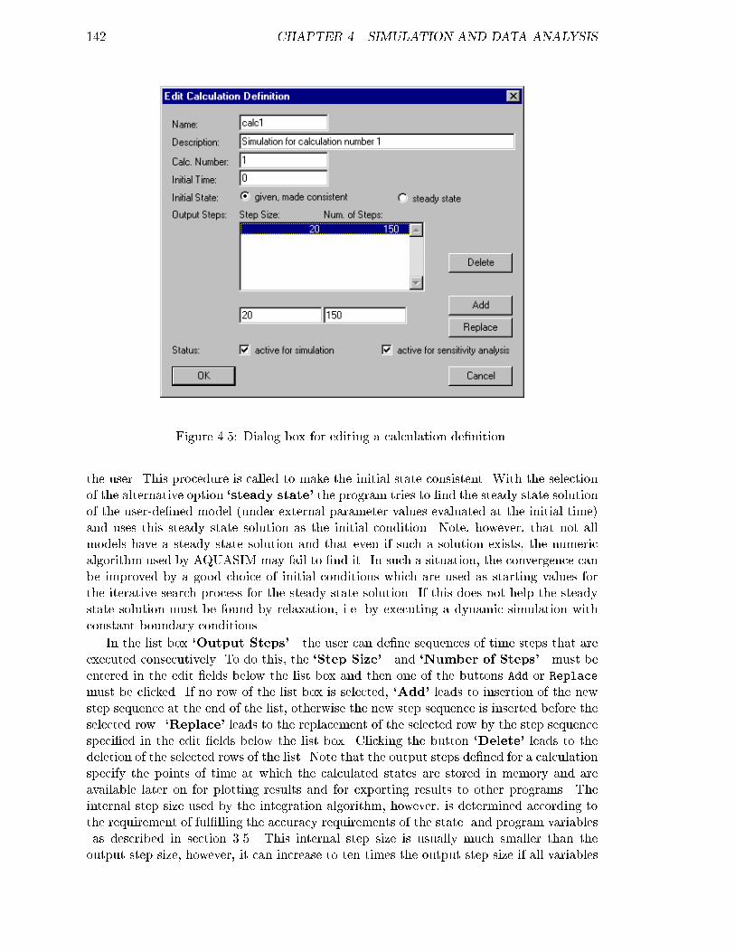
142 CHAPTER 4. SIMULATION AND DATA ANALYSIS
Figure 4.5: Dialog box for editing a calculation de�nition.
the user. This procedure is called to make the initial state consistent. With the selection
of the alternative option `steady state' the program tries to �nd the steady state solution
of the user-de�ned model (under external parameter values evaluated at the initial time)
and uses this steady state solution as the initial condition. Note, however, that not all
models have a steady state solution and that even if such a solution exists, the numeric
algorithm used by AQUASIM may fail to �nd it. In such a situation, the convergence can
be improved by a good choice of initial conditions which are used as starting values for
the iterative search process for the steady state solution. If this does not help the steady
state solution must be found by relaxation, i.e. by executing a dynamic simulation with
constant boundary conditions.
In the list box `Output Steps' the user can de�ne sequences of time steps that are
executed consecutively. To do this, the `Step Size' and `Number of Steps' must be
entered in the edit �elds below the list box and then one of the buttons Add or Replace
must be clicked. If no row of the list box is selected, `Add' leads to insertion of the new
step sequence at the end of the list, otherwise the new step sequence is inserted before the
selected row. `Replace' leads to the replacement of the selected row by the step sequence
speci�ed in the edit �elds below the list box. Clicking the button `Delete' leads to the
deletion of the selected rows of the list. Note that the output steps de�ned for a calculation
specify the points of time at which the calculated states are stored in memory and are
available later on for plotting results and for exporting results to other programs. The
internal step size used by the integration algorithm, however, is determined according to
the requirement of ful�lling the accuracy requirements of the state and program variables
as described in section 3.5. This internal step size is usually much smaller than the
output step size, however, it can increase to ten times the output step size if all variables

4.1. SIMULATION 143
change only smoothly in time (the solution at the output steps is then determined by
interpolation). The size of the internally used time step can be bounded as described
in section 3.5 (this may be useful in order to avoid that the algorithm steps over short
excitations).
Finally, the check boxes `active for simulation' and `active for sensitivity anal-
ysis' are used to activate the calculation for the speci�ed task.
During the execution of a simulation, the dialog box shown in Fig. 4.6 shows the
Figure 4.6: Dialog box for interrupting a simulation.
current calculation and the current simulation time and it allows the user to interrupt the
simulation.

144 CHAPTER 4. SIMULATION AND DATA ANALYSIS
4.2 Sensitivity Analysis
As mentioned in the introduction, sensitivity analysis combines the tasks of identifyability
analysis and uncertainty analysis.
The goal of identi�ability analysis is to check if model parameters can be uniquely
determined with the aid of the available data and to estimate the uncertainty of the pa-
rameter estimates. This can be done by estimating the standard errors and correlation
coe�cients of parameters during the parameter estimation procedure as described in sec-
tion 4.3. An additional source of information on the identi�ability of model parameters are
the sensitivity functions discussed in this section. The following four sensitivity functions
are distinguished by AQUASIM:
�a;ay;p =@y
@p(4.9a)
�r;ay;p =1
y
@y
@p(4.9b)
�a;ry;p = p@y
@p(4.9c)
�r;ry;p =p
y
@y
@p(4.9d)
y
p
y ( p )
p 2 p0
y
δ a , ry , p
δ a , ry , p
Figure 4.7: Interpretation of the absolute-relative sensitivity function �a;ry;p = p@y=@p.
In these functions, y is an arbitrary variable calculated by AQUASIM and p is a model
parameter represented by a constant variable or by a real list variable. The absolute-
absolute sensitivity function (4.9a) measures the absolute change in y per unit of change

4.2. SENSITIVITY ANALYSIS 145
in p, the relative-absolute sensitivity function (4.9b) measures the relative change in y
per unit of change in p, the absolute-relative sensitivity function (4.9c) measures the
absolute change in y for a 100 % change in p, and the relative-relative sensitivity function
(4.9d) measures the relative change in y for a 100 % change in p. All these changes are
calculated in linear approximation only. The most useful sensitivity functions are the
absolute-relative sensitivity function (4.9c) and the relative-relative sensitivity function
(4.9d), because their units do not depend on the unit of the parameter. This makes
quantitative comparisons of the e�ect of di�erent parameters p on a common variable y
possible. Because the relative-relative sensitivity function (4.9d) is non-dimensional, this
sensitivity function can not only be used to compare the e�ect of di�erent parameters
on a common variable, but also the e�ects of di�erent parameters on di�erent variables.
However, the disadvantage of this relative-relative comparison is that it gives not very
useful results if the value of the variable y becomes small during a simulation (because
large relative changes of a value that is close to zero are not relevant). Fig. 4.7 illustrates
the meaning of the absolute-relative sensitivity function (4.9c). The linear approximation
to the change in y for a 100 % change in p can easily be constructed with the aid of the
tangent to the function y(p) in p. The larger the values of sensitivity functions and the
more pronounced the di�erences in shape of the sensitivity functions (within the range of
available data), the more accurately are the parameters identi�able.
Figure 4.8 shows an example of the time dependence of the sensitivity functions of
Figure 4.8: Example of a plot of sensitivity functions of a calculated concentration with
respect to three model parameters.
a calculated concentration with respect to three model parameters K, rmax and Cini
(look at the tutorial for a complete description of this example). It is evident that the
parameter Cini is identi�able from measured concentrations, because for small values of the
time, t, the calculated concentration is only sensitive to this parameter. The sensitivity
functions of the parameters K and rmax have a similar shape (the signs indicate that
the calculated concentrations increase with increasing values of K, but they decrease

146 CHAPTER 4. SIMULATION AND DATA ANALYSIS
with increasing values of rmax). This leads to a correlation between the estimates of
these parameters (changes in calculated concentrations caused by a change in K can
approximately be compensated by an appropriate change in rmax). Furthermore, the much
smaller sensitivity of the calculated concentration to the parameter K in comparison to
the sensitivity to the parameter rmax leads to a larger uncertainty of the estimate of K
than that of rmax.
In uncertainty analysis, the uncertainty of model parameters is propagated to the
uncertainty of model results (model structure uncertainty is not addressed as an auto-
mated task of AQUASIM, however, predictions with di�erent model structures can be
compared manually). In the current version of AQUASIM only the simplest error prop-
agation method is implemented, the linearized propagation of standard devitions of un-
correlated parameters. The error propagation formula using the linearized model and
neglecting the parameter correlation is given by
�y =
vuut mXi=1
�@y
@pi
�2�2pi (4.10)
where pi are the uncertain model parameters, �pi are their standard deviations, y(p1; :::; pm)
is the solution of the model equations for a given variable at a given location and time,
and �y is the approximate standard deviation of the model result. Figure 4.9 shows a
Figure 4.9: Example of a plot of simulation results with estimated error bounds.
plot of measured data and the simulation result with error bounds limiting the range of
values of the result plus and minus one standard deviation. The error contribution of
each parameter is given as
�erry;p =@y
@p�p (4.11)

4.2. SENSITIVITY ANALYSIS 147
The error contributions of the three parameters of the example shown in the Figs. 4.8 and
4.9 are shown in Fig. 4.10. It is interesting that the magnitudes of the error contributions
Figure 4.10: Example of a plot of error contributions of three model parameters on a
calculated concentration.
due to the parameters K and rmax are of a similar size despite the di�erence in sensitivity
shown in Fig. 4.8. The reason for this e�ect is the higher uncertainty in the estimate of
K resulting form the smaller sensitivity.
The derivatives required for calculating the sensitivity functions (4.9a) to (4.9d), the
standard deviations of calculated variables according to equation (4.10), and the contri-
butions of parameter uncertainties to the total uncertainty according to equation (4.11)
are calculated using the �nite di�erence approximation
@y
@pi�
y(pi +�pi)� y(pi)
�pi(4.12)
where �pi is chosen to be 1 % of the standard deviation �pi of the parameter pi. In order
to make the program as exible as possible, the solutions for the basic parameter values
(p1; :::; pm) and for all sets of parameter values, where one of the pi's is replaced by pi+�piare calculated one after the other and stored simultaneously. Using these m + 1 stored
states, all the expressions (4.9a) to (4.9d), (4.10), and (4.11) can be evaluated easily for
any variable y.
Figure 4.11 shows the dialog box used for de�ning and starting a sensitivity analysis.
This dialog box is opened with the Sensitivity Analysis command in the Calc menu
shown in Figure 4.1.
The two upper two list boxes in this dialog box show the active and the available
`Parameters' (constant variables and real list variables), respectively. With the aid of
the buttons `Activate' and `Inactivate', parameters selected in the right list box can be

148 CHAPTER 4. SIMULATION AND DATA ANALYSIS
Figure 4.11: Dialog box for editing a sensitivity analysis.
activated and parameters selected in the left list box can be inactivated (this is equivalent
to toggle the check box active for sensitivity analysis in the dialog boxes shown
in Figs. 3.7 and 3.9).
The two lower list boxes show the active and the available `Calculations', respectively.
These are the same calculation de�nitions as are needed to execute simulations as described
in section 4.1. The buttons `New', `Duplicate', `Edit', and `Delete', used for editing
calculations, have the same functionality as the same buttons described for the dialog box
shown in Fig. 4.4 in section 4.1. The calculations are edited as described in section 4.1 with
the aid of the dialog box shown in Fig. 4.5. With the aid of the buttons `Activate' and
`Inactivate', calculations selected in the right list box can be activated and calculations
selected in the left list box can be inactivated (this is equivalent to toggle the check box
active for sensitivity analysis in the dialog box shown in Fig. 4.5).
The button `Start' is used to start the sensitivity analysis, the button `Close' to
close this modeless dialog box. After clicking the button Start the user is asked to specify
the name of a �le for a sensitivity ranking. If the user clicks Cancel in the �le open dialog
box, no sensitivity ranking is produced (this may be advantageous to save computation
time if the ranking is not required). During execution of the sensitivity analysis the dialog
box shown in Fig. 4.12 is displayed. This dialog box shows the progress of the calculation
and it allows the user to interrupt the sensitivity analysis. When all simulations have
been performed and if a sensitivity ranking �le has been speci�ed, the dialog box shown
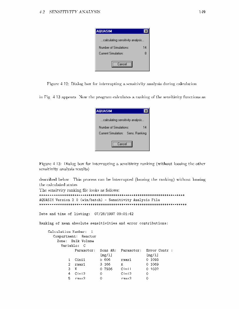
4.2. SENSITIVITY ANALYSIS 149
Figure 4.12: Dialog box for interrupting a sensitivity analysis during calculation.
in Fig. 4.13 appears. Now the program calculates a ranking of the sensitivity functions as
Figure 4.13: Dialog box for interrupting a sensitivity ranking (without loosing the other
sensitivity analysis results).
described below. This process can be interrupted (loosing the ranking) without loosing
the calculated states.
The sensitvity ranking �le looks as follows:***********************************************************************
AQUASIM Version 2.0 (win/batch) - Sensitivity Analysis File
************************************************************************
Date and time of listing: 07/28/1997 09:01:42
Ranking of mean absolute sensitivities and error contributions:
Calculation Number: 1
Compartment: Reactor
Zone: Bulk Volume
Variable: C
Parameter: Sens AR: Parameter: Error Contr.:
[mg/l] [mg/l]
1 Cini1 5.606 rmax1 0.1093
2 rmax1 3.166 K 0.1069
3 K 0.7936 Cini1 0.1032
4 Cini2 0 Cini2 0
5 rmax2 0 rmax2 0

150 CHAPTER 4. SIMULATION AND DATA ANALYSIS
Calculation Number: 2
Compartment: Reactor
Zone: Bulk Volume
Variable: C
Parameter: Sens AR: Parameter: Error Contr.:
[mg/l] [mg/l]
1 Cini2 0.0769 K 0.0071
2 rmax2 0.0632 rmax2 0.0031
3 K 0.0530 Cini2 0.0030
4 rmax1 0 rmax1 0
5 Cini1 0 Cini1 0
It gives a ranking of the averages of the absolute values of the absolute-relative sensitivity
functions (4.9c) and of the error contributions (4.11) for all state variables in all zones of
all compartments and for all calculations. For models with many parameters, this ranking
is very useful to quickly �nd out which are the most important parameters in uencing the
state variables in the di�erent compartments.

4.3. PARAMETER ESTIMATION 151
4.3 Parameter Estimation
Model parameters represented by constant variables can be estimated by AQUASIM by
minimizing the sum of the squares of the weighted deviations between measurements and
calculated model results
�2(p) =
nXi=1
�ymeas;i � yi(p)
�meas;i
�2(4.13)
In this equation ymeas;i is the i-th measurement, �meas;i is its standard deviation, yi(p)
is the calculated value of the model variable corresponding to the i-th measurement and
evaluated at the time and location of this measurement, p = (p1; :::; pm) are the model
parameters, and n is the number of data points. The measurements ymeas;i (for i = 1; :::; n)
must be represented by real list variables with the argument either the program variable
Time or the program variable corresponding to the space coordinate of the compartment
in which the comparison takes place. The standard deviations �meas;i can be de�ned
individually for each data point or globally for all data points of each real list variable
in the dialog box used for editing real list variables shown in Fig. 3.9. The sum (4.13)
extends over all data points of all real list variables speci�ed as �t targets as shown below.
Simultaneous comparisons of data for measurements corresponding to di�erent variables,
compartments and zones are possible. AQUASIM performs a minimization of the sum of
squares (4.13) with the constraints
pmin;i � pi � pmax;i (4.14)
where pmin;i and pmax;i are the minimum and maximum of the constant variable repre-
senting pi. The values for pmin;i and pmax;i are speci�ed in the dialog box used for editing
constant variables shown in Fig. 3.7.
Due to the possible nonlinearity of the model equations and due to the numerical inte-
gration procedure, the sum (4.13) must be minimized numerically. The user has the choice
between two numerical minimization algorithms: The simplex algorithm (Nelder and
Mead, 1965) and the secant algorithm (Ralston and Jennrich, 1978). Both of these tech-
niques are well-suited for the minimization of numerically integrated equations, because
they avoid the calculation of derivatives of the solutions with respect to the parameters.
The simplex technique starts with a set of m + 1 (m is the number of parameters)
arrays of parameter values buildung a simplex with nonzero volume in parameter space
(in AQUASIM, this set consists of one array with the user-de�ned start values and m
arrays in which exactly one parameter value di�ers from its start value). At each iteration
step, the simplex of arrays of parameter values is replaced by a new simplex according
to the following strategy (Nelder and Mead, 1965) illustrated in Fig. 4.14 for the case
of two parameters to be estimated. The parameter array leading to the highest value
of �2 is �rst re ected at the plane de�ned by the other parameter arrays (see Fig. 4.14
(1); this is a rough guess for the downhill direction). If the value of �2 at this re ected
array of parameter values is between the lowest and the highest value of the old simplex,
this re ected array of parameter values is accepted and replaces the array leading to the
highest value of �2. If the value of �2 at the re ected parameter array is smaller than
the lowest value on the old simplex, a new parameter array with an increased step size is
calculated (see Fig. 4.14 (2)) by an expansion of the simplex. If the value of �2 at this

152 CHAPTER 4. SIMULATION AND DATA ANALYSIS
( 1 ) r e f l e c t i o n ( 2 ) r e f l e c t i o n a n d e x p a n s i o n
( 3 ) c o n t r a c t i o n i n o n e d i m e n s i o n ( 4 ) c o n t r a c t i o n i n a l l d i m e n s i o n s
h i g h
l o w
h i g h
l o w
h i g h
l o w
h i g h
l o w
Figure 4.14: Basic steps of the simplex algorithm for function minimization illustrated
for the case of two parameters. The solid line simplex is replaced by one of the hashed
simplexes.
new array of parameter values is smaller than the lowest value on the old simplex it is
accepted, otherwise the re ected array (without expansion) is accepted (in both cases the
new array replaces the array leading to the highest value of �2 of the old simplex). If the
value of �2 at the re ected point is higher than the highest value at the old simplex, a
new array of parameter values is constructed by contracting the point with the highest
value of �2 of the old simplex in direction to the other points of the simplex (see Fig.
4.14 (3)). If this leads to a value of �2 that is smaller than the highest value at the old
simplex, this array is accepted, otherwise, all arrays of parameter values of the old simplex
with exception of that leading to the lowest value of �2 are contracted in direction to the
array leading to the lowest value (see Fig. 4.14 (4)). This procedure is repeated until all
values of �2 at the points of the simplex are close enough together in order to ful�ll the
convergence criterion. This unconstrained simplex technique is extended to constrained
minimization by the coordinate transformation of the parameters
p0i = tan
��
2
2pi � pmax;i � pmin;i
pmax;i � pmin;i
�(4.15)
shown in Fig. 4.15. Application of the unconstrained technique to the parameters p0iis equivalent to constrained minimization of the parameters pi. If the (unconstrained)
estimates of the parameters p0i are found the parameters pi can be calculated by the
inverse formula
pi =1
2(pmax;i + pmin;i) + (pmax;i � pmin;i)
arctan(p0i)
�(4.16)
Similarly to the simplex technique described above, the secant technique starts with
a set of m+ 1 arrays of parameters. But now the secant technique uses the special form
of the function �2 (4.13) to be minimized. There is exactly one linear function in the
parameters that passes through all function values yi(p) for all m + 1 parameter sets.
For this linear function, the expression (4.13) is a quadradic form with exactly one well-
de�ned minimum. The idea of the secant technique (Ralston and Jennrich, 1978) is to

4.3. PARAMETER ESTIMATION 153
p i '
p i '
p m i n , i p m a x , i
p ip i
Figure 4.15: Scaled tan-function used to transform the bounded interval pmin;i; pmax;i of
the parameter pi to the whole real axis for the parameter p0
i.
replace one of the m+1 parameter arrays with the array leading to the minimum for the
linear approximation of the model functions yi(p) at each iteration step. In order to take
into account the constraints of the parameters, the secant technique was combined with
the active set technique (Gill et al., 1981) for the implementation in AQUASIM. In the
active set technique the inequality constraints (4.14) are replaced by a number of (active)
equality constraints for which some of the parameters are exactly on one of their boundary
values. After each iteration step, this set of active constraints is checked for validity and
changes to this set are made if this seems to be necessary.
Because it looks for a downward direction in a very robust way, the simplex technique
may be applied even to a poorly de�ned parameter estimation process with starting values
of the parameters far from those leading to the minimum of (4.13). In contrast, the secant
method has more problems with bad starting values and poorly de�ned minima of �2, but
it leads to much faster end convergence close to a well-de�ned minimum. Estimates for
the standard errors of the estimated parameters and for the parameter correlation matrix
are only calculated by the secant method, and only if no parameter estimated is on one of
the bounds pmin;i or pmax;i of the parameter.
Figure 4.16 shows the dialog box used for de�ning and starting a parameter estimation.
This dialog box is opened with the Parameter Estimation command in the Calc menu
shown in Figure 4.1.
The two upper list boxes in this dialog box show the active and the available `Pa-
rameters' to be estimated (constant variables), respectively. With the aid of the buttons
`Activate' and `Inactivate', parameters selected in the right list box can be activated
and parameters selected in the left list box can be inactivated (this is equivalent to tog-

154 CHAPTER 4. SIMULATION AND DATA ANALYSIS
Figure 4.16: Dialog box for editing a parameter estimation.
gle the check box active for parameter estimation in the dialog box used for editing
constant variables shown in Fig. 3.7).
The two lower list boxes show the active and the available `Calculations', respec-
tively. The calculation de�nitions for parameter estimation can be edited with the aid
of the buttons `New', `Duplicate', `Edit' and `Delete' as discussed below. With the
aid of the buttons `Activate' and `Inactivate', calculations selected in the right list box
can be activated and calculations selected in the left list box can be inactivated (this is
equivalent to toggle the check box active for parameter estimation in the dialog box
shown in Fig. 4.17).
The radio buttons `secant' and `simplex' can be used to select the numerical
minimization `Method' above. The basic ideas and references for both possible selections
are given above.
In the edit �eld `Maximum Number of Iterations', the number of iterations can
be bounded. A value of zero leads to the calculation of the value of �2 without trials to
improve this value.
The button `Start' is used to start the parameter estimation, the button `Close' to
close this modeless dialog box. After clicking the button Start the user is asked to specify

4.3. PARAMETER ESTIMATION 155
the name of a �le on which the parameter and �2 values for all iteration steps are reported
and which contains a �nal summary of parameter estimates, estimated standard errors
and correlation coe�cients (for the secant method not leading to estimates on the bounds
of the constraining interval only), and a list of the contributions of each data series to the
total value of �2 (see below for an example of such a �le).
As discussed above, the buttons New, Edit and Duplicate in the dialog box shown in
Fig. 4.16 are used to de�ne calculations for parameter estimation. Figure 4.17 shows the di-
alog box used for de�ning and editing a single calculation. The items Name, Description,
Figure 4.17: Dialog box for editing a parameter estimation calculation.
Calc. Number, Initial Time and Initial State have the same meaning as for calcula-
tions for simulation and sensitivity analysis in the dialog box shown in Fig. 4.5:
The edit �eld `Name' is used to specify the name of the calculation. Each calculation
needs a unique name as an identi�er. A name of a calculation consists of a sequence of
letters (A-Z,a-z), digits (0-9) and underline characters ( ). The �rst character may not be
a digit.
To improve documentation of calculations the edit �eld `Description' can optionally
be used to store comments on the purpose of the calculation de�nition.
The edit �eld `Calc. Number' allows the program user to identify a calculation by
a nonnegative integer number. Variables (and thus also processes, etc.) can be made
dependent on this calculation number with the aid of the program variable Calculation
Number. Active calculations must have di�erent values of their calculation numbers.
Each calculation must be initialized before it can be started. In the edit �eld `Initial
Time' the time at which a calculation is initialized can be speci�ed.
The user has the choice between two types of the `Initial State' to be used by

156 CHAPTER 4. SIMULATION AND DATA ANALYSIS
the program. The default option `given, made consistent' applies the initial state as
given by the user (a value of zero is the default initial condition for all state variables for
which the user did not explicitly specify an initial condition). If this initial state violates
constraints on boundary conditions or algebraic equations of equilibrium processes, the
program tries to ful�ll these constraints by a minimal number of modi�cations to the initial
state given by the user. This procedure is called to make the initial state consistent. With
the selection of the alternative option `steady state' the program tries to �nd the steady
state solution of the user-de�ned model (under external parameter values evaluated at the
initial time) and uses this steady state solution as the initial condition. Note, however,
that not all models have a steady state solution and that even if such a solution exists,
the numeric algorithm used by AQUASIM may fail to �nd it. In such a situation, the
convergence can be improved by a good choice of initial conditions which, under this
option for the initial state, are used as starting values for the iterative search process for
the steady state solution. If this does not help, the steady state solution must be found
by relaxation, i.e. by executing a dynamic simulation with constant boundary conditions.
After these �ve items which have the same meaning as those discussed for simulation
and sensitivity analysis (Fig. 4.5), instead of step sizes and numbers of steps, the user
must specify Fit Targets (the step sizes are selected automatically by the program to
meet the points in time at which data are available). All �t targets already de�ned are
listed in the list box of the dialog box shown in Fig. 4.17. Each �t target consists of a data
series and a speci�cation of which variable evaluated in which zone of which compartment
and at which point in time or space should be compared with the data. The list of �t
targets is edited with the buttons `Add', `Edit' and `Delete' below the list box.
Finally, the calculation can be made `active for parameter estimation', if no other
calculation with the same calculation number is already active.
The Fig. 4.18 shows the dialog box used to specify a �t target. This dialog box is
Figure 4.18: Dialog box for editing a �t target.
opened by clicking one of the buttons Add or Edit of the dialog box shown in Fig. 4.17.
In the �rst �eld `Data' of this dialog box a data series can be selected. This data
series is represented by a real list variable with the argument either the program variable
Time or the program variable corresponding to the space coordinate of the compartment
in which the comparison with the calculated variable takes place.

4.3. PARAMETER ESTIMATION 157
The next four �elds of the dialog box shown in Fig. 4.18 are used to de�ne which
calculated value of the model should be compared with the data series speci�ed in the
�rst �eld.
In the �eld `Variable', a variable must be selected. In many cases measured data
is compared with values of a state variable of the model, but in AQUASIM, any variable
can be used. E.g. a formula variable can be used for conversion of units, for building
combinations of state variables (e.g. a sum of state variables that is measured), etc..
In the �eld `Compartment' the compartment must be selected in which the variable
to be compared with the data has to be evaluated. This �eld is inactive if there exists
only one compartment.
In the �eld `Zone' the zone of the compartment must be selected in which the variable
to be compared with the data has to be evaluated. This �eld is inactive if there exists
only one zone in the compartment selected above.
In the last �eld Time/Space the time must be speci�ed at which the comparison of
the spatial pro�le data with the calculated variable, or the spatial location at which the
comparison with the time series data must take place. Note that the value entered here
is interpreted as a spatial location if the argument of the real list variable selected in the
�eld Data is the program variable Time, and as a point of time if the argument of the real
list variable selected in the �eld Data is the program variable corresponding to the spatial
location of the compartment selected in the �eld Compartment. If the check box `relative
space' is ticked, spatial locations must be given in relative coordinates, otherwise in
absolute coordinates (this check box has no in uence for time speci�cations which are
always absolute). In the case of a comparison with time series data, the value entered in
the �eld Time/Space must be within the legal coordinate range of the compartment. For
absolute spatial locations, the legal range is de�ned in the de�nition of the compartment
selected in the �eld Compartment. Relative locations must be between 0 and 1. If the
compartment is a mixed reactor compartment (which has no spatial coordinate), the value
entered in the �eld Time/Space is ignored.
During execution of the parameter estimation the dialog box shown in Fig. 4.19 is
displayed. This dialog box shows the initial value of �2, the best (smallest) value already
Figure 4.19: Dialog box for interrupting a parameter estimation.
found, and the value for the current parameter set. This dialog box allows the user to
interrupt the calculation.

158 CHAPTER 4. SIMULATION AND DATA ANALYSIS
In case of normal termination of the parameter estimation algorithm, the dialog box
shown in Fig. 4.20 is displayed to give the user a brief survey of the �t results. The �rst
Figure 4.20: Dialog box for displaying a summary of �t results.
row of this dialog box shows the termination status of the algorithms, the second row the
number of iterations performed. In the following list box for each parameter that was
active for parameter estimation, its initial value, its �nal value (found by the parameter
estimation algorithm), and its minimum and maximum is given. Finally, below the list
box, the initial and the �nal value of �2 are given in order to give the user a quick overview
on the improvement that could be achieved by the parameter estimation procedure.
More details on the performance of the parameter estimation algorithm is given on the
�le speci�ed after clicking the button Start in the dialog box shown in Fig. 4.16. This
�le looks as follows:
***********************************************************************
AQUASIM Version 2.0 (win/mfc) - Parameter Estimation File
************************************************************************
Date and time of listing: 07/29/1997 13:56:09
Number of parameters = 5
Number of data points = 22
Estimation method = secant
Parameters:
Name Unit Start Minimum Maximum
Cini1 mg/l 12 0 20
Cini2 mg/l 0.8 0 2
K mg/l 2 0 10
rmax1 mg/l/h 2 0 10
rmax2 mg/l/h 2 0 10

4.3. PARAMETER ESTIMATION 159
Calculations:
Cini1 Cini2 K rmax1 rmax2 Chi^ 2
[mg/l] [mg/l] [mg/l] [mg/l/h] [mg/l/h]
12 0.8 2 2 2 1749.41
12.2 0.8 2 2 2 1700.74
12 0.82 2 2 2 1725.51
12 0.8 2.1 2 2 1656.36
12 0.8 2 2.1 2 1928.34
12 0.8 2 2 2.1 1795.93
11.9411 0.80557 2.3 2.01325 2.01687 1516.94
11.8094 0.82432 2.9 2.06794 2.13019 1191.95
. . . . . .
. . . . . .10.1604 1.00113 1.04662 1.04293 0.51529 22.6634
10.1531 1.00421 1.03489 1.03858 0.51681 22.5086
Parameter estimation successfully finished (convergence criterion met)
Cini1 Cini2 K rmax1 rmax2
[mg/l] [mg/l] [mg/l] [mg/l/h] [mg/l/h]
Estimated values of the parameters:
10.1531 1.00421 1.03489 1.03858 0.51681
Estimated standard errors of the parameters:
0.22133 0.03057 0.27284 0.07084 0.09739
Estimated correlation matrix of the parameters:
1 0.17923 0.53889 0.77737 0.52576
0.17923 1 0.34116 0.30991 0.46943
0.53889 0.34117 1 0.92990 0.98009
0.77737 0.30991 0.92990 1 0.901655
0.52576 0.46943 0.98009 0.90166 1
Contribution of data series to Chi^ 2
Calculation: Data Series: Chi^ 2 ini: Chi^ 2 end:
Fit1 Cmeas1 801.34 12.1706
Fit2 Cmeas2 948.074 10.338
------- -------
1749.41 22.5086
Number of steps performed = 27
Number of simulations performed = 39
After the header, on this �le the number of parameters and the number of data points
active for the current parameter estimation and the method selected for the numerical min-

160 CHAPTER 4. SIMULATION AND DATA ANALYSIS
imization algorithm are indicated. Then the �le contains a listing of all active parameters
with unit, start value, minimum and maximum. Then a listing of the parameter values and
of the values of �2 for all calculations performed during the parameter estimation process
is given. After this listing, the parameter estimates are given. If the estimation algorithm
was the secant method and no parameter estimate was on the border of its legal range,
an estimate of the standard error and of the parameter correlation matrix is also given.
Then, in addition to the value of �2 which represents the sum of the deviations for all �t
targets, the contributions of all �t targets to the �nal value of �2 are given individually.
Finally, the number of iterative steps and the number of simulations performed, are given.

Chapter 5
Visualization of Results
Fig. 5.1 shows the menu View of AQUASIM. The item `Results' of this menu is used
Figure 5.1: View menu.
to specify plot de�nitions, to plot results to the screen or in PostScript or Encapsulated
PostScript format to a �le, and to list results to a text �le for external postprocessing. The
item `Toolbar' is used to activate or hide the AQUASIM toolbar, and the item `Status
Bar' is used to activate or hide the status bar of AQUASIM (the status bar is not used
in the current version of AQUASIM).
Figure 5.2 shows the dialog box used for editing plot de�nitions and for plotting and
listing results. This dialog box is opened with the command Results of the menu View
shown in Fig. 5.1. The list box in this dialog box contains a list of plot de�nitions.
Each of these plot de�nitions contains general plot speci�cations such as meaning, labels
and scaling of axes and a list of curves to be drawn in the plot. Each of these curves
contains speci�cations such as the type of the curve (value, sensitivity function or error
contribution of a variable), the variable, the calculation number, the compartment, the
161

162 CHAPTER 5. VISUALIZATION OF RESULTS
Figure 5.2: Dialog box for editing plot de�nitions and plotting and listing results.
zone, the spatial location (if the abscissa of the plot is time) or the time (if the abscissa
of the plot is the spatial coordinate of the compartment) at which the curve should be
drawn, and the signature of the curve. All these de�nitions can be speci�ed independently
of the existence of the calculated states necessary for actually drawing the curves. The
recommended strategy is therefore to spend some time to carefully specify a series of
plot de�nitions which can later on be used very e�ciently to present an overview of the
current simulation results. The buttons at the right of the list box of plot de�nitions
allow the user to perform the following operations: By clicking the button `New', new
plot de�nitions can be speci�ed. Alternatively, by clicking the button `Duplicate', the
selected plot de�nition can be duplicated. With the button `Edit', or by double-clicking
the plot de�nition name in the list box, a plot de�nition can be edited. The button
`Delete' allows the program user to delete plot de�nitions. The buttons Duplicate, Edit
and Delete are inactive as long as no plot de�nition is selected. The dialog boxes used
for editing plot de�nitions are discussed later in this section (Figs. 5.3 to 5.5).
The three buttons `Plot to Screen', `Plot to File', and `List to File' are used to
draw a plot corresponding to the currently selected plot de�nition to the screen, to write
it in PostScript or Encapsulated PostScript format to a �le, and to write it in text format
to a �le, respectively. The PostScript or Encapsulated PostScript �le must be handled by
the user. Typically, a PostScript �le is sent to a printer with the aid of an appropriate
program (available as a shareware program), an Encapsulated PostScript �le is included
as a �gure into a text processing program. All the three actions described above are only
possible, if calculated data for at least one curve of the currently selected plot de�nition
exists and if no curve contains unde�ned values as they can occur e.g. by division by zero
or by taking logarithms of negative numbers in the variable to be plotted.
The three buttons `Scr. Opt.', `File Opt.', and `List Opt.' are used to specify

163
general options for plotting to the screen, for plotting to a PostScript �le, and for listing
plot data to a text �le, respectively. The dialog boxes used for specifying these options
are discussed later in this section (Figs. 5.6 to 5.8).
Figure 5.3 shows the dialog box used for de�ning or editing a plot de�nition. This
Figure 5.3: Dialog box for editing a plot de�nition.
dialog box is opened by clicking one of the buttons New, Edit or Duplicate of the dialog
box shown in Fig. 5.2.
Each plot de�nition needs a unique `Name' as an identi�er. A name of a plot
de�nition consists of a sequence of letters (A-Z,a-z), digits (0-9) and underline characters
( ). The �rst character may not be a digit. To improve documentation of plot de�nitions,
a `Description' can be given optionally.
The edit �eld `Title' is used to specify the title of the plot.
The radio buttons `Abscissa' can be used to select the meaning of the abscissa. The
user has the choice between the abscissa `Time' which is used for plotting time series
at given locations in the system described with AQUASIM and the absissa `Space' used
for plotting spatial pro�les at given points of time (this last option is not meaningful for
mixed reactors that have no spatial variation in state variables).
The edit �elds `Label' can be used to specify a label for the Abscissa and for the
Ordinate, respectively.
A plot de�nition contains an arbitrary number of de�nitions of `Curves'. All curve
de�nitions are listed in the list box of the dialog box shown in Fig. 5.3. The buttons `Add',
`Edit' and `Delete' below this list box are used to edit the list of curve de�nitions. If no

164 CHAPTER 5. VISUALIZATION OF RESULTS
curve de�nition is selected, clicking the button Add leads to the insertion of a new curve
de�nition at the end of the list of curve de�nitions. If a curve de�nition is selected, the
new curve de�nition is inserted before the selected curve de�nition.
Finally, the button `Scaling' is used to choose options for bounds and ticks of the axes
of the plot.
Figure 5.4 shows the dialog box used for de�ning or editing a curve de�nition within
a plot. This dialog box is opened by clicking one of the buttons Add or Edit of the dialog
Figure 5.4: Dialog box for editing the de�nition of a curve within a plot.
box shown in Fig. 5.3.
The radio buttons `Type' are used to select the type of the curve. The user has the
choice between the following options: The radio button `Value' is selected in order to
plot the value of a variable. The value of all variables can be plotted if calculated states
corresponding to the speci�cations given below are available. If not only a simulation,
but a sensitivity analysis has been performed, the curve for the value of the variable is
supplemented by thin lines indicating the value plus and minus one standard deviation
calculated according to the linear error propagation formula which ignores parameter
correlations (4.10). Usually, if the abscissa of the plot is Time, the curve for the value of
a variable is plotted as linear interpolation between values evaluated at each output time
step speci�ed in the dialog box shown in Fig. 4.5 (for plots drawn after a simulation or a

165
sensitivity analysis) or by the time steps of the data speci�ed as �t targets in the dialog
box shown in Fig. 4.18 (for plots drawn after a parameter estimation). If the abscissa of
the plot is Space, similarly the grid points of the spatial resolution of the compartment
are used. There is one important exception from this general rule: If the abscissa of the
plot is Time and the variable speci�ed in the curve de�nition is a real list variable with
the program variable Time as the argument, or if the abscissa of the plot is Space and the
variable specifed in the curve de�nition it is a real list variable with the program variable
corresponding to the spatial extent of the compartment as the argument, the data pairs
of the real list are used instead of the interpolated values at the simulation times or grid
points. This makes it possible to plot measured data without interpolation (see alsow
Figs. 5.9 and 5.10). Selection of one of the radio buttons `Error Contrib.' and `Sens.
Function' leads only to a curve if a sensitivity analysis corresponding to the speci�cations
below has been performed. Selection of the radio button Error Contrib. leads to the
plot of the error contribution of a parameter p to the total error of a variable y given by
equation (4.11). Selection of the radio button Sensitivity Function leads to the plot
of a sensitivity function. Selection of the radio button `AbsAbs' leads to the plot of the
absolute-absolute sensitivity function given by equation (4.9a), selection of `RelAbs' to
the plot of the relative-absolute sensitivity function given by equation (4.9b), selection of
`AbsRel' to the plot of the absolute-relative sensitivity function given by equation (4.9c),
and selection of `RelRel' to the plot of the relative-relative sensitivity function given by
equation (4.9d).
Figure 5.5: Dialog box for editing scaling of plot axes.
As a next item in the dialog box used for the speci�cation of a curve de�nition shown
in Fig. 5.4, a `Variable' must be selected.
If the type of the curve is Error Contrib. or Sensitivity Function, a constant
variable or a real list variable must be selected as a `Parameter'. The curve can then
only be plotted, if a sensitivity analysis with this Parameter as an active parameter has
been performed. This �eld is inactive, if the curve is of the type Value.
The edit �eld `Calculation Number' is used to select a calculation identi�ed by
its calculation number (speci�ed in one of the dialog boxes shown in Figs. 4.5 and 4.17).

166 CHAPTER 5. VISUALIZATION OF RESULTS
Because calculations for di�erent calculation numbers can be stored in memory simulta-
neously and because variables and process rates can be made depend on the calculation
number with the aid of the program variable Calculation Number, curves for the same
variable at the same location under di�erent process hypotheses can be compared in the
same plot.
As a next speci�cation, a `Compartment' within which the curve must be evaluated
can be seleced. This �eld is inactive if only one compartment is de�ned.
If the compartment selected above contains more than one zone, a `Zone' must be
selected. This �eld is inactive if the compartment contains only one zone.
Figure 5.6: Dialog box for editing plot to screen options.
Finally, the edit �eld `Time/Space' is used to complete the speci�cation of when and
where to evaluate the curve. If the abscissa of the plot is Time, a spatial location valid for
the compartment selected above must be given here. If the check box `rel. space' is ticked,
relative coordinates between 0 and 1 must be given, otherwise absolute spatial locations
must be speci�ed. The values of the variable of function to be plotted are then linearly
interpolated between the values at the neighbouring grid points of the compartment. In
the case of a mixed reactor compartment, the value of this edid �eld is ignored, because
there is no spatial resolution. If the abscissa of the plot is Space the edit �eld Time/Space
is used to specify the time at which the curve is evaluated. In this case the check box rel.
space is ignored (points in time must always be given as absolute values). The values are
linearly interpolated between the neighbouring output time steps speci�ed in one of the
dialog boxes shown in Figs. 4.5 and 4.17.
In the edit �eld `Legend' the user can specify a legend entry for the curve.
The appearance of the curve can be speci�ed by `Line' and `Marker' attributes.
The check boxes `active' are used to turn on and o� the lines between data pairs and
the markers at the data pairs, respectively. As described above, the data pairs of plots
with the abscissa Time are usually determined by the output time steps of the calculation,
the data pairs of plots with the abscissa Space by the grid points of the compartment.
If the value of a real list variable with the program variable corresponding to the space
coordinate of the compartment as its argument is plotted in a plot with the abscissa Time,
or if the value of a real list variable with the program variable Time as its argument is
plotted in a plot with the abscissa Space, instead, the data pairs of the real list variable

167
Figure 5.7: Dialog box for editing plot to �le options.
are used. In order to plot the actually used interpolated values (that may be di�erent
from linear interpolation according to the selection of the Interpolation Method in the
dialog box shown in Fig. 3.9), a formula variable with the name of the real list variable as
its algebraic expression may be de�ned and speci�ed as the variable to be plotted (this is
in fact the way the data for the plot shown in Fig. 3.8 has been generated). Several line
attributes, grouped as `Style', `Width' and `Color' attributes, can be used to obtain
a clear distinction between plotted curves. Similarly, for markers, `Style', `Size' and
`Color' attributes are available.
Figure 5.5 shows the dialog box used to specify the scaling of the plot. This dialog
box is opened by clicking the button Scaling of the dialog box shown in Fig. 5.3.
For both, `Abscissa' and `Ordinate', a `Minimum', a `Maximum', a `Tick Po-
sition' and a `Tick Distance' can either be speci�ed or selected to be automatically
determined. The possibility of specifying a tick position makes the positions of the ticks
independent of the bounds of the axis.
Figure 5.6 shows the dialog box used to edit the options for plotting to the screen.
This dialog box is opened by clicking the button Scr. Opt. of the dialog box shown in
Fig. 5.3.
It allows the program users to specify the `Width' and the `Height' of the plot
window, the width of the `Margins' and the `Legend Width'. In addition, the user can
select the `Font Size' for the plot `Title', for the axes `Labels', for the `Legend' and
for the tick `Numbers'. All measurement units are pixels.
Figure 5.7 shows the dialog box used to edit the options for plotting in PostScript

168 CHAPTER 5. VISUALIZATION OF RESULTS
Figure 5.8: Dialog box for editing list to �le options.
or Encapsulated PostScript format to a �le. This dialog box is opened by clicking the
button File Opt. of the dialog box shown in Fig. 5.3.
It allows the program user to select the `Paper Size' and the `Orientation' and to
specify the number of `Columns' and `Rows' of plots on the sheet, the `Margins', the
`Legend Width' and the `Font Size' for the `Title', the axes `Labels', the `Legend'
and the tick `Numbers'.
Furthermore, the user can select to plot in `color' or `black/white', to use `cm' or
`inch' as measurement units for distances and to select `PostScript' or `Encapsulated
PostScript' as the �le format (PostScript is suited for printing, Encapsulated Postscript
for including AQUASIM plots in other documents).
Figure 5.9: Example of a plot window on the screen.
Figure 5.8 shows the dialog box used to edit the options for listing calculated results
corresponding to a plot de�nition to a text �le. This dialog box is opened by clicking the

169
button List Opt. of the dialog box shown in Fig. 5.3.
The user can select the number of `Signi�cant Digits' and the Separator between
numbers on the output �le.
Figure 5.9 shows a plot window on the screen. This plot window is generated by
clicking the button Plot to Screen in the dialog box shown in Fig. 5.2. It contains four
curves. Two of them, represented by markers, are real list variables with the program
variable Time as the argument. In this case, the data pairs of the real list variables are
plotted. The other two curves, represented by a dashed and a solid line, respectively, are
simulation results and are plotted with a high temporal resolution. Figure 5.10 shows
the same plot written in Encapsulated PostScript format to a �le and imported to this
document. This �le is obtained by selecting the option Encapsulated PostScript in the
dialog box shown in Fig. 5.7 and then clicking the button Plot to Screen in the dialog
box shown in Fig. 5.2. Finally, the following listing shows the plot of two of the curves
shown above as obtained by clicking the button List to File in the dialog box shown in
Fig. 5.2.
3e+0032e+0031e+0030
0.6
0.5
0.4
0.3
0.2
0.1
0
Production
time [s]
Prod
[m
gO/l/
h]
90uE/m2/s
1300uE/m2/s
90uE/m2/s
1300uE/m2/s
Figure 5.10: Example of an Encapsulated PostScript plot.

170 CHAPTER 5. VISUALIZATION OF RESULTS
************************************************************************
AQUASIM Version 2.0 (win/mfc) - List File
************************************************************************
Date and time of listing: 05/05/1998 11:47:00
Name of plot: Val Prod
Type: Argument Value Argument Value
Variable: t Prod1 t Prod
Parameter:
CalcNum: 0 1Compart.: Reactor Reactor
Zone: Bulk Volume Bulk Volume
Time/Space: 0 0Unit: s mgO/l/h s mgO/l/h
Legend: 90uE/m2/s 90uE/m2/s
150 0.095 0 0300 0.16 20 0.01492600 0.16 40 0.02858900 0.14 60 0.041061200 0.13 80 0.052481500 0.13 100 0.062911800 0.13 120 0.072462100 0.13 140 0.08118
160 0.08915180 0.09644200 0.1031220 0.1092240 0.1147260 0.1198280 0.1244300 0.1286320 0.1325340 0.136360 0.1392380 0.1421400 0.1447420 0.1471440 0.1493460 0.1513480 0.1531500 0.1548. .. .

Chapter 6
Appendix
6.1 Character Interface Version
Besides the window interface version of AQUASIM described in the other sections of this
manual, there exists a character interface version with the same functionality exept that
it is not able to draw plots to the screen. This version is designed for editing AQUASIM
system �les and for executing simulations, sensitivity analyses and parameter estimations
via simple character-oriented terminal connections and for automating editing tasks with
the aid of scripts of the operating system. For normal usage of the program, the window
interface version is much more attractive.
Because the menu and dialog structure of the character interface version is exactly the
same as that of the window interface version, the other chapters of this manual can be used
as a manual for the character interface version also. In the following, some speci�c hints on
the usage of the character interface version are given and a simple example demonstrates
how to start and exit the character interface version.
In the character interface version, user input is prompted with a sign `>' and each user
input must be followed by pressing `Return'. Menu items have to be selected by typing
the number preceeding the item and pressing `Return'. Within menus and submenus,
`Return' without giving an input before leads back to the previous menu level. Default
values proposed in square brackets can be accepted by pressing `Return' without giving a
new input before.
The following sequence shows how to start and exit the character interface version of
AQUASIM (the two menus correspond to the menu bar of the window shown in Fig. 1.1
and to the menu File shown in Fig. 2.1):
171

172 CHAPTER 6. APPENDIX
>aquasimc
***********************************************
* *
* AQUASIM - Simulation of Aquatic Systems *
* *
***********************************************
AQUASIM - Main Menu
-------------------
1 = File
2 = Edit
3 = Calc
4 = View
>1
AQUASIM - File Menu
-------------------
1 = New
2 = Open
3 = Close
4 = Save
5 = Save As
6 = Revert to Saved
7 = Print
8 = About
E = Exit
B = Back
>e
End of program AQUASIM (normal termination)

6.2. BATCH VERSION 173
6.2 Batch Version
The batch version of AQUASIM is designed for executing demanding calculations on a
compute server as batch jobs. In contrast to the window and character interface versions
of AQUASIM, the batch version does not provide full functionality. In particular, it is
not possible to de�ne or edit models. The idea of the batch version is to perform one of
the following tasks for a model de�ned with the aid of an interactive program version and
stored on an AQUASIM system �le:
� Perform a simulation.
� Perform a sensitivity analysis.
� Perform a parameter estimation.
� Calculate values of �2.
� Calculate results for given parameter sets and given variables.
� Plot results to a PostScript or Encapsulated PostScript �le.
� List results to a text �le.
On systems for which command line arguments can be speci�ed, these jobs can be
started with the following command lines
aquasimb jobfile
aquasimb -s logfile loadfile savefile [scmdfile]
aquasimb -a logfile loadfile savefile [sensfile]
aquasimb -e logfile loadfile savefile fitfile
aquasimb -c logfile loadfile vcmdfile chifile
aquasimb -r logfile loadfile vcmdfile rcmdfile resfile
aquasimb -p logfile loadfile pcmdfile
aquasimb -l logfile loadfile lcmdfile
The parameters used in these command lines have the following meaning:
jobfile AQUASIM job �le. This �le can contain one or more command lines in
the style of the other command lines. These command lines are executed
one after the other so that a job speci�ed in a command line can use
the save�le of one of the previous jobs as its load�le. When used within
such a job �le, the program name aquasimb may be omitted and the line
can directly start with -s, -a, -e, -c, -p or -l. Within a job �le a #-
sign terminates input for the current line and makes it possible to add
comments.
-s Perform a simulation.
-a Perform a sensitivity analysis.
-e Perform a parameter estimation.
-c Perform a calculation of �2-values.
-r Calculate results for given parameter sets and given variables.
-p Plot results to a PostScript �le.

174 CHAPTER 6. APPENDIX
-l List results to a text �le.
logfile Name of an output text �le for job log information. The information
written to this �le may be useful in case of problems during calculation
(CAUTION: an existing �le with this name is overwritten without warn-
ing!).
loadfile Name of the input AQUASIM system �le containing the model de�nitions.
This �le must be created with one of the interactive program versions.
savefile Name of an output AQUASIM system �le on which the results are stored.
This �le can be opened with an interactive program version or from a
succeeding batch job for processing results (CAUTION: an existing �le
with this name is overwritten without warning!).
scmdfile Name of an (optional) input text �le (simulation command �le) containing
the instructions for initialization and step sizes of simulations. If no such
�le is provided, the active calculations speci�ed in the simulation dialog
box are executed. If a simulation command �le is provided, for each calcu-
lation number for which simulations should be performed, a line providing
the two numbers
calcnum inittime
(calcnum = calculation number, inittime = initial time) must be pro-
vided. This line is followed by an arbitrary number of lines of the form
calcnum timestep numsteps
(calcnum = calculation number, timestep = output step size for time
integration, numstes = numper of steps to be performed).
sensfile Name of an (optional) output text �le to which a ranking of mean absolute
sensitivity and error functions is written (CAUTION: an existing �le with
this name is overwritten without warning!).
fitfile Name of an output text �le to which detailed results of the parameter
estimation are written (CAUTION: an existing �le with this name is over-
written without warning!).
vcmdfile Name of an input text �le (parameter value �le) specifying the names and
values of parameters. The �rst line of this �le must contain the names
of the parameters (constant variables), on succeeding lines values of these
parameters must be speci�ed, each line containing one set of values for all
parameters (the value of each parameter must be within the legal range
of the parameter bounded by its minimum and maximum).
chifile Name of an output text �le to which the results of the calculations of
�2-values are written. After a header, each line of this �le contains the
parameter values and the corresponding value of �2 (CAUTION: an ex-
isting �le with this name is overwritten without warning!).
rcmdfile Name of an input text �le (result de�nition �le) de�ning when and where
to calculate results. This �le must contain lines of the following form:
var calcnum comp zoneind time space relabs
where var is the name of a variable, calcnum is the calculation number of
an active calculations, comp is the name of a compartment, zoneind is an
allowed zone index for this compartment, time is a point of time within

6.2. BATCH VERSION 175
the simulation time range, space is a location within the compartment,
and relabs is equal to the letter `a' for absolute space coordinates or
equal to the letter `r' for relative space coordinates. The space coordinate
must also be speci�ed for mixed reactor compartments, however, in this
case its value is ignored.
resfile Name of an output text �le to which the results of the calculations are
written. After a header, each line of this �le contains the parameter values
and the corresponding values for all result de�nitions speci�ed in the result
de�nition �le (CAUTION: an existing �le with this name is overwritten
without warning!).
pcmdfile Name of an input text �le (plot command �le) specifying the names of
the plot de�nitions that are used to generate plots and the �le names to
which the plots are written (in PostScript format). A plot command �le
contains an arbitrary number of lines of the form
plot psfile
where plot is the name of a plot de�nition and psfile is the name of a
PostScript �le to which the plot is appended.
lcmdfile Name of an input text �le (list command �le) specifying the names of
the plot de�nitions that are used to generate listings of results and the �le
names to which these results are written (in ascii format). A list command
�le contains an arbitrary number of lines of the form
plot lisfile
where plot is the name of a plot de�nition and lisfile is the name of a
text �le to which the results are appended.
If the batch version of AQUASIM is started without command line arguments (e.g. on
systems that do not support this feature) the program looks for a �le aquasim.job in the
current directory. If it �nds such a �le, this �le is interpreted as an AQUASIM job �le, if
no �le with this name exist, the programs terminates with an error message.
As an example, an AQUASIM job �le containing the lines
-e fit1.log test.aqu test res.aqu test1.fit
-e fit2.log test res.aqu test res.aqu test2.fit
-e fit3.log test res.aqu test res.aqu test3.fit
-s sim.log test res.aqu test res.aqu sim.cmd
-p plot.log test res.aqu plot.cmd
executes a parameter estimation based on the AQUASIM system �le test.aqu, restarts
this estimation twice, then for the �tted parameter values starts a simulation according to
the speci�cation given in the simulation command �le sim.cmd (e.g. for improving the plot
resolution) and plots the results according to the speci�cations given in the plot command
�le plot.cmd to PostScript �les.

176 CHAPTER 6. APPENDIX
6.3 Troubleshooting
AQUASIM was developed in the computer and systems sciences department of EAWAG
primarily for internal use. Since EAWAG is an institution for research and teaching and
not a software company, it is not possible for us to provide end-user support. Instead, the
following possibilities are o�ered:
� In this chapter hints are given for self-diagnosis and solution of problems (section
6.3.1).
� A user group is maintained as an e-mail list through which questions can be sent
to other AQUASIM users. In this way, AQUASIM users can �nd help within the
user community of AQUASIM (section 6.3.2).
� Bug reports and suggestions for program improvements are welcome at any time.
Although there is no technical support on program use, we try to �x all bugs and
provide bug-�xed program versions to licensed program users (section 6.3.3).
� Courses on AQUASIM use are given occasionally at EAWAG.
A topical overview of AQUASIM-related information, such as on the most recent program
version, on references of program applications, on planned AQUASIM courses, and on
known bugs or problems can be found on the EAWAG home page at http://www.eawag.ch.

6.3. TROUBLESHOOTING 177
6.3.1 Problem Self-Diagnosis
In this subsection, hints are given for how to �nd the cause of problems in program use.
In the �rst subsection, problems of loading AQUASIM system �les are discussed, in the
second subsection problems of editing models, and in the third subsection problems during
calculations.
Problems of Loading Files
Format of AQUASIM System Files
Before discussing possible problems of loading �les, in this paragraph some explanations to
the �le format used by AQUASIM are given. In order to guarantee compatibility between
di�erent operating systems, AQUASIM systems are stored as ASCII text �les. Line breaks
guarantee compatibility with �le editors and with e-mail programs. During the loading
process all special characters (ASCII code below 32, e.g. line break and carriage return
characters) are stripped from the �le and the �le is converted to a simple character stream
(this is important because line breaks are represented di�erently on di�erent operating
systems). AQUASIM items are structured with the aid of curly braces (f and g). Text
between two successive opening or closing braces is ignored, only text between an opening
and a closing brace of the same level without any braces in between is interpreted by
AQUASIM. A program convedit (convert AQUASIM system �le for editing with a text
editor) is provided with AQUASIM (in the subdirectory bin) which converts the originally
more compact �le format to a format that is much easier to read (line breaks and indents
are inserted at each opening brace and between closing braces of di�erent level) and is
equivalent for AQUASIM (there is no tool to reverse this process, because this is not
necessary since AQUASIM can read the converted �le; the original format can easily be
restored by loading and saving the �le with AQUASIM). This tool may be used to allow
advanced AQUASIM users to analyse causes for �le loading problems or even to edit
an AQUASIM system �le directly with a text editor or a programming language (e.g.
with Perl scripts). This last possibility may be e�cient for the automation of repeated
complicated editing processes. However, it is also dangerous, because with the aid of a
text editor or a scripting language minor errors can make a �le unreadable by AQUASIM.
Problems During the Loading Process
The most important cause for problems in loading �les is that a �le from one of the very
old versions AQUASIM 1.0x or from a newer AQUASIM version than that used for loading
is tried to be loaded. Files from AQUASIM 1.0x must be converted to the �le format for
AQUASIM 1.1 with the aid of the conversion program conv1011 which is delivered with
AQUASIM (in the subdirectory bin). Files from AQUASIM 1.1x and from pre-releases
of AQUASIM 2.0 can then be read by AQUASIM 2.0, however, it is not possible to save
a system in an older �le format with AQUASIM 2.0. Files from newer versions than
AQUASIM 2.0 cannot be loaded with AQUASIM 2.0.
AQUASIM system �les are compatible between all operating systems supported by
AQUASIM. One problem may occur on the Mac if an AQUASIM system �le is transferred
to the Mac from another operating system. If the �le type is not AQU , the �le is not
displayed in the �le open dialog box of AQUASIM. For this reason, after the transfer to
the Mac, the �le type must be set to this value (AQUASIM system �les created on the
Mac automatically obtain this �le type). This can be done in various ways:

178 CHAPTER 6. APPENDIX
� The �le is moved on the application AQUASIM Typer which is delivered with the
Mac distribution of AQUASIM.
� The �le is loaded with the character interface version of the Mac and saved by
this program version.
� The �le type is changed to AQU with another tool, e.g. with the Mac resource
editor.
After a parameter estimation, the estimated standard deviations may become unde-
�ned (due to inversion of an ill-de�ned matrix). On some operating systems (especially on
the Mac), we did not succeed in �nding a function to check for such unde�ned values. If on
these systems such an unde�ned value is saved on the AQUASIM system �le, AQUASIM
is not able to read this value during loading. Because the save �le format of AQUASIM is
a text �le, such an unde�ned value can be found with a text editor and can be corrected
(see comments on the �le format above). The string indicating an unde�ned value may
depend on the operating system (e.g. NaN).

6.3. TROUBLESHOOTING 179
Problems of Editing a Model
Errors of two major types can occur during model editing: Errors assigned to an edit �eld
of the active dialog box and more general errors of incompatibility of the newly edited
structure with the rest of the system de�nitions.
Errors assigned to an edit �eld can usually easily be identi�ed. Figure 6.1 shows an
example of such an error. The error message indicates an error in the edit �eld Expression.
Figure 6.1: Example of an error assigned to an edit �eld of the dialog box.
If this error message occurs it is recommended to �rst check the existence of all variables
used in the edit �eld and to check the correctness of the algebraic expression. In the
present case (Fig. 6.1), as is seen in the dialog box Edit Variables in the background,
the variable x used in the algebraic expression of the formula variable does not exist.
If syntax and existence checks do not help uncovering the problem, it is recommended
to carefully read the explanating text to the referenced edit �eld in the user manual.
Besides errors in algebraic equations, illegal dependencies may occur. Examples of illegal
dependencies are use of a program variable that is not meaningful in the context of the
current compartment or the absence of obligatory dependencies.
Inconsistency errors of the newly de�ned object with existing system de�nitions are
more di�cult to �nd. In many cases, as shown in the example shown in Fig. 6.2, the name
of the object may already exist. Also in this case, it is recommended to carefully read the
comments to the dialog box in the user manual.

180 CHAPTER 6. APPENDIX
Figure 6.2: Example of an error assigned to an edit �eld of the dialog box.

6.3. TROUBLESHOOTING 181
Problems During Calculation
The Log File of AQUASIM
The most important source of information on problems during calculation is the log �le of
AQUASIM. For each interactive section, a log �le aquasim.log is written to the program
directory of AQUASIM (the log �le from the previous session is overwritten). As explained
in section 6.2 for batch jobs, the user can specify the name of the log �le in the command
line or in the job �le. The contents of the log �le can usually be ignored. However, it
may contain useful information in case of problems during calculations. The following
listing shows a typical log �le written during an interactive simulation of the activated
sludge example delivered with AQUASIM and described in section 8.2 of the report on
the concepts of AQUASIM (Reichert, 1994b).
************************************************************************
AQUASIM Version 2.0 (win/mfc) - Log File
************************************************************************
Start of Session: 05/12/1998 20:58:43
Calculation of consistent initial condition
-------------------------------------------
Number of codiagonals considered: 1000Time of initial condition: -50
05/12/1998 22:03:04 Start of calculation
05/12/1998 22:03:04 End of calculation
Number of equations: 50Number of integers needed for calculation: 50Number of reals needed for calculation: 5400
Number of steps taken: 0
Number of evaluations of the jacobian: 0
Dynamic calculation
-------------------
Number of codiagonals considered: 1000Maximum internal step size: 1
05/12/1998 22:03:04 Start of calculation
05/12/1998 22:03:04 Integration at time -50
05/12/1998 22:03:07 Integration at time -49.98
05/12/1998 22:03:08 Integration at time -49.96
05/12/1998 22:03:08 Integration at time -49.94
05/12/1998 22:03:08 Integration at time -49.92
05/12/1998 22:03:08 Integration at time -49.9
.
.

182 CHAPTER 6. APPENDIX
05/12/1998 22:03:13 Integration at time 0.9
05/12/1998 22:03:13 Integration at time 0.92
05/12/1998 22:03:13 Integration at time 0.94
05/12/1998 22:03:13 Integration at time 0.96
05/12/1998 22:03:13 Integration at time 0.98
05/12/1998 22:03:13 Integration at time 1
05/12/1998 22:03:13 End of calculation
Number of equations: 50Number of integers needed for calculation: 70Number of reals needed for calculation: 2990
Current integration time: 1.0055Current step size: 0.00915549Current order of integration: 3Number of steps taken: 420Number of function evaluations: 864Number of evaluations of the jacobian: 48Number of error test failures: 10Number of convergence test failures: 2
First, information on the initialization process is given. The value of the numerical param-
eter, Number of Codiagonals of the Jacobian Matrix (cf. section 3.5), and the time
at which the initial condition is evaluated, are given.
Then, start time and end time of the initialization procedure are given.
As a next group of parameters, the number of equations solved by the numerical
algorithm and the memory requirements for the initialization process, expressed as a
number of integer variables and a number of real variables, are listed.
The number of steps and the number of evaluations of the jacobian matrix required for
the calculation of the initial state conclude the information on the initialization process.
Information on dynamic calculations starts with the values of the numerical parameters
Number of Codiagonals of the Jacobian Matrix and Maximum Internal Step Size
(cf. section 3.5).
The next block of information shows the time consumption of the simulation by giving
the time at each output time step.
As a next group of parameters, the number of equations solved by the numerical
algorithm and the memory requirements for the application of the di�erential-algebraic
system solver DASSL (Petzold, 1983), expressed as a number of integer variables and a
number of real variables, are listed.
The next block of information shows the current (at the end of the simulation) values
of integration time, step size and integration order, gives a summary on the number of
integration steps taken, of function evaluations and of evaluations of the jacobian matrix,
and gives the numbers of error test failures and convergence test failures of the algorithm
DASSL (Petzold, 1983). Especially these last two numbers may be interesting for simu-
lation performance improvements. An error test failure indicates that the algorithm tries
to perform a too large time step and it has to repeat the step with a smaller step size in
order to ful�ll the accuracy criteria of all state and program variables (cf. section 3.5).
A change of the accuracies of state and program variables (cf. section 3.5) may decrease
the number of error test failures. A convergence test failure indicates that the algorithm
had to decrease the size of the time step because it was not able to �nd the solution of

6.3. TROUBLESHOOTING 183
the nonlinear system of algebraic equations for the solution after the time step (the iter-
ative equation solver did not converge; cf. section 4.1). One cause for a large number of
convergence test failures may be a too low value of the numerical parameter Number of
Codiagonals of the Jacobian Matrix.
Problems of Wrong Calculation Results
Due to the robustness of the integration algorithm used by DASSL (Petzold, 1983) it is very
rare that wrong simulation results occur. To our knowledge the only cases in which wrong
calculation results occur are cases related to the automatic selection of integration time
steps. If the integration time step is large in comparison to a short term change in system
behaviour, the algorithm may step over such a change in behavior. The consequence of
this problem is that the change in behaviour is not recognised by the calculation.
There are two very important examples of this problem. The �rst is related to short-
term external excitation of a system, the second to short term changes in process rates
due to changes in the values of variables calculated from the solution.
a) If the driving forces of a system (process rates and inputs) usually only vary slowly
in time but show some short-term excitations, then, during the slow variation phase, the
integration algorithm gradually increases the size of its time step. If then a short-term
excitation with a duration shorter than the time step occurs, the algorithm may hit the
excitation or it may step over the excitation. In the �rst case the algorithm recognises the
integration problem and it follows the excitation accurately by decreasing the integration
step size appropriately. In the second case the algorithm steps over the excitation without
recognising it and the simulation result becomes erroneous. The simplest way of solving
this problem is to decrease the value of the maximum internal step size of the integration
algorithm to a value smaller than the duration of the excitation as described in section
3.5. If this slows down the integration too much during the smooth behaviour periods, an
alternative may be to decrease the output time step to a value smaller than one tenth of
the duration of the excitation during the excitation only (this also leads to better results
for the plots), and let the output time step to be large during the smooth periods. This
also works because the size of the internal time step is not allowed to increase to values
larger than ten times the output time step.
b) If changes in reaction rates may occur abruptly as a function of a variable calculated
by the program (e.g. a calculated concentration), a similar problem as described under a)
may occur. The di�erence of the present problem to the one described above is that the
time at which it occurs is unknown. This makes the second solution procedure proposed
above inapplicable (decreasing the time step only in the critical ranges of time). The
�rst solution (decreasing the internal time step) may improve the results, however, the
appropriate size of the time step is more di�cult to estimate, because it depends on
the time scale of changes of the values of system variables which are calculated by the
program. For this reason and to make the integration faster, it is better to solve this
problem by changing the formulation of the rate expressions in a way that makes the
problem detectable by the integration algorithm. This procedure is illustrated with a
simple example: A rate expression of Monod type
r =rmaxC
K + C; (6.1)
where r is the degradation rate of the substance described by the concentration C, rmax
is the maximum degradation rate and K is the concentration at which the degradation

184 CHAPTER 6. APPENDIX
rate is half of its maximum value, may cause such a problem if the value of K is very
small in comparison to typical initial values of C and if degradation continues to zero. For
large concentrations (C >> K) the degradation rate is approximately equal to rmax, for
decreasing concentrations it tends to zero. However, for large negative concentrations, the
degradation rate is also equal to rmax. If now the integration algorithm makes huge time
steps because the decrease of C with a constant rate rmax is very simple to integrate, the
concentration may jump over the whole range of small and negative rates to large negative
values of C, where the rate is again approximately equal to rmax, and the degradation
process continues (to larger negative values of C). This problem only occurs if typical
concentrations C are much larger than K and a fast decrease of C to zero is possible. An
elegant way to solve this problem is to extend the function given above in a di�erent way
to negative concentrations (to avoid the problem that again rmax is returned). If the rate
is extended linearly by
r =
8><>:
rmaxC
K + Cfor C � 0
rmax
KC for C � 0
(6.2)
the problem is avoided without changing the function in the domain of (resonable) pos-
itive concentrations C. If now the algorithm steps to negative concentrations, it obtains
negative degradation rates that di�er signi�cantly from the positive value of rmax. Such
a rapid change in the rate during a single time step is not acceptable for the error test
criterion and the step size is decreased. For this reason, the correct smooth approach to
zero is achieved and negative concentrations do not occur in the �nal model results (they
may only occur during integration steps that are not accepted).
In most cases, errors in the user input are the cause for wrong simulation results. It is
advantageous to print out the system de�nitions and to check these de�nitions carefully
in order to �nd the cause of the problem. In addition it may be advantageous to plot
important system variables that do not show correct behaviour and to turn o� processes
one after the other in order to �nd out which process caused the problem. Then this
process can be studied in more detail.
Problems of Integration Interrupts
If the integration algorithm detects a serious problem that cannot be solved by reducing
the integration step size and order, the integration process is interrupted with the message
box shown in Fig. 6.3. If this dialog box appears, in most cases there will be a message on
Figure 6.3: Example of a dialog box indicating a numerical problem.
the log �le of AQUASIM that may give hints with respect to the nature of the problems.

6.3. TROUBLESHOOTING 185
Two types of error should be distinguished: Error messages by the integration algorithm
DASSL (Petzold, 1983) which start with the keyword `DASSL' and error messages by
AQUASIM. Some examples of such error messages are discussed in the following two
subsections.
DASSL Errors
DASSL errors are more di�cult to interpret than AQUASIM errors because no speci�c
reference to AQUASIM system de�nitions can be given.
The DASSL error message
05/13/1998 15:27:39 Start of calculation05/13/1998 15:27:39 Integration at time 0DASSL{ AT CURRENT T = 0.00990773 1000 STEPSDASSL{ TAKEN ON THIS CALL BEFORE REACHING TOUT.05/13/1998 15:27:39 End of calculation
indicates that more time steps are required to reach the next point of output time than was
speci�ed as the value of the numerical parameter Maximum Number of Internal Time
Steps for One External Time Step (in the present example, the value of this param-
eter was set equal to 1000; cf. section 3.5). This limitation of the number of internal steps
for one external step was made in order to show numerical problems without loosing too
much computing time. Under usual circumstances the requirement for more than 1000
internal steps for one external step indicates the existence of a numerical problem. There
are two important exceptions from this general rule: If a dynamic simulations starts with
a relaxation to an equilibrium state and this is done with one output step only (because
the relaxation dynamics is not of interest), a large number of internal steps may be re-
quired in order to calculate the single external output step. The message shown above may
also appear during a parameter estimation, for which a simulation could be run without
problems. This is the case if the temporal distance between data points is much larger
than the output interval selected for the simulation. For such cases it is necessary to
increase the numerical parameter Maximum Number of Internal Time Steps for One
External Time Step as discussed in section 3.5. In other cases it may be more appro-
priate to try to �nd out why the integration algorithm performs poorly (with very small
time steps).
The DASSL error message that is most di�cult to interpret is the following:
05/13/1998 15:32:44 Start of calculation05/13/1998 15:32:44 Integration at time 005/13/1998 15:32:44 Integration at time 0.105/13/1998 15:32:44 Integration at time 0.205/13/1998 15:32:44 Integration at time 0.305/13/1998 15:32:44 Integration at time 0.405/13/1998 15:32:44 Integration at time 0.505/13/1998 15:32:44 Integration at time 0.605/13/1998 15:32:44 Integration at time 0.705/13/1998 15:32:44 Integration at time 0.805/13/1998 15:32:44 Integration at time 0.9DASSL{ AT T = 1 AND STEPSIZE H = 2.06912e-024DASSL{ THE ERROR TEST FAILED REPEATEDLYDASSL{ OR ABS(H) = HMIN.05/13/1998 15:32:44 End of calculation

186 CHAPTER 6. APPENDIX
This or a similar error message results if the algorithm repeatedly tried to reduce the
integration step size without being able to ful�ll the error test criterion. It is then the
di�cult task of the program user to �nd the cause of the numerical problem. The point
in time at which the problem occurs may help to �nd the cause. A rate or an input could
be discontinuous at this point in time. It may be useful to look at time series plots of
important system variables in order to detect strange behaviour at this point in time. It
may also be useful to change the accuracy of program and state variables in order to �nd
out if the problem occurs always at the same time (cf. section 3.5).
AQUASIM Errors
In most cases it is easier to �nd the cause for AQUASIM error messages. The following
example shows an error message that occurs when in the advective-di�usive compartment
a negative di�usion coe�cient is speci�ed:
05/13/1998 15:44:46 Start of calculationADVCOMP numerical problem: Di�usion coe�cient is not positive05/13/1998 15:44:46 End of calculation
If the error message is not clear enough, it is recommended to read the section of the user
manual in which the edit �eld of the referenced quantity is described.

6.3. TROUBLESHOOTING 187
6.3.2 Finding Help in the AQUASIM User Group
In order to facilitate communication on program use and application among AQUASIM
users, an electronic user group is maintained at the EAWAG mail server.
To join the AQUASIM user group, send the mail message
subscribe aquasim-users <mail-address>
to
In the mail message <mail-address>must be replaced by the mail address that should be
added to the user group. Because the mail is processed automatically, it is very important
that the mail message has exactly the format given above and does not include any further
comments. The text must be given in the body of the message and not as a subject. In
order to leave the AQUASIM user group send the mail message
unsubscribe aquasim-users <mail-address>
to
Your mail address is then deleted from the user group list.
Questions to be distributed or responses to distributed questions (that should again
be distributed) must then be sent to
All messages sent to this address are automatically distributed to all members of the list.
Usually, it is recommended to send your responses to distributed questions also to the user
group in order to allow all user group members to participate in the discussion. However,
individual answers to the person who sent out the question, are also possible.

188 CHAPTER 6. APPENDIX
6.3.3 Reporting Program Bugs and Suggestions for Improvements
Please report program errors as well as suggestions for program improvements to Peter Re-
ichert, EAWAG, CH-8600 D�ubendorf, Switzerland, or by email to [email protected].
An accurate description of the error accompanied by an AQUASIM system �le which leads
to the problem is very important.
We will provide information on known program errors, on workarounds and on bug-
�xed program versions on the EAWAG home page at http://www.eawag.ch.

Bibliography
Albrecht, A., Reichert, P., Beer, J., and L�uck, A. (1995). Evaluation of the importance of
reservoir sediments as sinks for reactor-derived radionuclides in riverine systems. J.
Environ. Radioactivity, 28(3):239{269.
Amorocho, J. and de Vries, J. (1980). A new evaluation of the wind stress coe�cient over
water surface. J. Geophys. Res., 85:433{442.
Arcangeli, J.-P. and Arvin, E. (1997a). Modelling of the cometabolic biodegradation of
trichloroethylene by toluene-oxidizing bacteria in a bio�lm system. Environmental
Science & Technology, 31:3044{3052.
Arcangeli, J.-P. and Arvin, E. (1997b). Modelling of the growth of a methanotrophic
bio�lm. Water Science and Technology, 36(1):199{204.
Beaudoin, D., Bryers, J., Cunningham, A., and Peretti, S. (1997). Mobilization of broad
host range plasmid from Pseudomonas putida to established bio�lms of Bacillus azoto-
formans. II. modeling. Biotechnology & Bioengineering, 57(3):280{286.
B�uhrer, H. and Amb�uhl, H. (1975). Die Einleitung von gereinigtem Abwasser in Seen.
Schweizerische Zeitschrift f�ur Hydrologie, 37:347{369.
Burchard, H. and Baumert, H. (1995). On the performance of a mixed-layer model based
on the k-� turbulence closure. J. Geophys. Res., 100(C5):8523{8540.
Chow, V. (1959). Open-channel hydraulics. McGraw-Hill, New York.
de St. Venant, M. (1871). Th�eorie du mouvement non permanant des eaux crues des
rivi�eres et �a l'introduction des mar�ees dans leur lit. Comptes Rendus, 73:147{154 &
237{240.
Eisenbeis, M., Bauer-Kreisel, P., and Scholz-Muramatsu, H. (1997). Studies of the dechlo-
rination of tetrachloroethene to cis-1,2-dichloroethene by dehalospirillium multivorans
in bio�lms. Water Science and Technology, 36(1):191{198.
Fesch, C., Lehmann, P., Haderlein, S., Hinz, C., Schwarzenbach, R., and Fl�uhler, H.
(1998a). E�ect of water content on solute transport in aggregated porous media. J.
Contaminant Hydrology, 33(1-2):211{230.
Fesch, C., Simon, W., Reichert, P., Haderlein, S., and Schwarzenbach, R. (1998b). Non-
linear sorption and nonequilibrium transport of organic contaminants in saturated
porous media: experiments, process identi�cation and modeling. J. Contaminant
Hydrology, 31(3-4):373{407.
189

190 BIBLIOGRAPHY
Filipe, C. and Daigger, G. (1997). Development of a revised metabolic model for the growth
of phosphorus-accumulating organisms. Water Environment Research, 70(1):67{79.
Fischer, H., List, E., Koh, C., Imberger, J., and Brooks, N. (1979). Mixing in Inland and
Coastal Waters. Academic Press, New York.
French, R. (1985). Open-channel hydraulics. McGraw-Hill, Stuttgart. New York.
Gear, C. (1971a). Algorithm 407, DIFSUB for solution of ordinary di�erential equations.
Communications ACM, 14(3):185{190.
Gear, C. (1971b). The automatic integration of ordinary di�erential equations. Commu-
nications ACM, 14(3):176{179.
Gear, C. (1971c). Numerical initial value problems in ordinary di�erential equations.
Prentice Hall, Stuttgart. Englewood Cli�s, N.J.
Gill, P., Murray, W., and Wright, M. (1981). Practical Optimization. Academic Press,
London.
Glod, G., Angst, W., Holliger, C., and Schwarzenbach, R. (1997a). Corrinoid-mediated
reduction of Tetrachloroethene, Trichloroethene, and Trichloro uoroethene in homo-
geneous aqueous solution: Reaction kinetics and reaction mechanisms. Environ. Sci.
Technol., 31:253{260.
Glod, G., Brodmann, U., Angst, W., Holliger, C., and Schwarzenbach, R. (1997b).
Cobalamin-mediated reduction of cis- and trans-dichloroethene, 1,1-dichloroethene,
and vinyl chloride in homogeneous aqueous solution: reaction kinetics and mechanis-
tic considerations. Environ. Sci. Technol., 31:3154{3160.
Goudsmit, G.-H., Reichert, P., and W�uest, A. (1996). Modelling of physical and bio-
geochemical properties in lakes using AQUASIM. In M�uller, A., editor, Hydroinfor-
matics 96, pages 779{786. Balkema, Rotterdam.
Gujer, W. and Wanner, O. (1990). Modeling mixed population bio�lms. In Characklis, W.
and Marshall, K., editors, Bio�lms, pages 397{443. John Wiley & Sons, New York.
Henderson, F. (1966). Open channel ow. Macmillan, New York.
Henze, M., Grady, C., Gujer, W., Marais, G., and Matsuo, T. (1986). Activated sludge
model no. 1. Scienti�c and Technical Report 1, IAWPRC Task Group on Math-
ematical Modelling for Design and Operation of Biological Wastewater Treatment
Processes, IAWPRC, London.
Hindmarsh, A. (1983). ODEPACK. a systematized collection of ODE solvers. In Steple-
man, R., editor, Scienti�c Computing, pages 55{64. IMACS / North-Holland.
Horn, H. and Hempel, D. (1995). Mass transfer coe�cients for an autotrophic and a
heterotrophic bio�lm system. Wat. Sci. Tech., 32(8):199{204.
Horn, H. and Hempel, D. (1997). Substrate utilization and mass transfer in an autotrophic
bio�lm system: Experimental results and numerical simulation. Biotechnology and
Bioengineering, 53(4):363{371.
BIBLIOGRAPHY 191
Jancarkova, I., Larsen, T., and Gujer, W. (1997). Distribution of nitrifying bacteria in a
shallow stream. Water Science and Technology, 36(8-9):161{166.
Janning, K., Harremo�es, P., and Nielsen, M. (1995). Evaluating and modelling the kinetics
in a full scale submerged denitri�cation �lter. Wat. Sci. Tech., 32(8):115{123.
Kuba, T., Murnleitner, E., van Loosdrecht, M., and Heiijnen, J. (1996). A metabolic
model for biological phosphorus removal by denitrifying orgnisms. Biotechnology and
Bioengineering, 52(6):685{695.
LeVeque, R. J. (1990). Numerical Methods for Conservation Laws. Birkh�auser, Basel.
Londong, J., Borchardt, D., Firk, W., Reichert, P., Stein, M., and Strotmann, U. (1994).
Nitrit in Fliessgew�assern. Korrespondenz Abwasser, 11/94:2069{2076.
Maryns, F. and Bauwens, W. (1997). The application fo the activated sludge model no. 1
to a river environment. Water Science and Technology, 36(5):201{208.
Mirpuri, R., Sharp, W., Villaverde, S., Jones, W., Lewandowski, Z., and Cunningham, A.
(1997). Predictive model for Toluene degradation and microbial phenotypic pro�les in
at plate vapor phase bioreactor. Journal of Environmental Engineering, 6/97:586{
592.
Murnleitner, E., Kuba, T., van Loosdrecht, M., and Heiijnen, J. (1997). An integrated
metabolic model for the aerobic and denitrifying biological phosphorus removal.
Biotechnology and Bioengineering, 54(5):434{450.
Musvoto, E., Wentzel, M., Loeventhal, R., and Ekama, G. (1997). Kinetic-based model
for mixed weak acid/base systems. Water SA, 23(4):311{322.
Nelder, J. and Mead, R. (1965). A simplex method for function minimization. Computer
Journal, 7:308{313.
Novack, B. and Sigg, L. (1997). Dissolution of Fe(II)(hydr)oxides by metal-EDTA com-
plexes. Geochimica et Cosmochimica Acta, 61(5):951{963.
Peeters, F., Kipfer, R., Hohmann, R., Hofer, M., Imboden, D., Kodenev, G., and Khozder,
T. (1997). Modeling transport rates in lake Baikal: Gas exchange and deep water
renewal. Environ. Sci. Technol., 31:2973{2982.
Petersen, E. (1965). Chemical Reaction Analysis. Prentice-Hall, Englewood Cli�s, New
Jersey.
Petzold, L. (1983). A description of DASSL: A di�erential/algebraic system solver. In
Stepleman, R. e., editor, Scienti�c Computing, pages 65{68. IMACS / North-Holland,
Amsterdam.
Ralston, M. and Jennrich, R. (1978). DUD - a derivative-free algorithm for nonlinear least
squares. Technometrics, 20(1):7{14.
Reichert, P. (1994a). AQUASIM - A tool for simulation and data analysis of aquatic
systems. Wat. Sci. Tech., 30(2):21{30.

192 BIBLIOGRAPHY
Reichert, P. (1994b). Concepts underlying a computer program for the identi�cation and
simulation of aquatic systems. Schriftenreihe der EAWAG 7, Swiss Federal Institute
for Environmental Science and Technology (EAWAG), CH-8600 D�ubendorf, Switzer-
land.
Reichert, P. (1995). Design techniques of a computer program for the identi�cation of
processes and the simulation of water quality in aquatic systems. Environmental
Software, 10(3):199{210.
Reichert, P. (1998). AQUASIM 2.0 { Tutorial. Technical report, Swiss Federal Institute for
Environmental Science and Technology (EAWAG), CH-8600 D�ubendorf, Switzerland.
Reichert, P., von Schulthess, R., and Wild, D. (1995). The use of AQUASIM for estimating
parameters of activated sludge models. Wat. Sci. Tech., 31(2):135{147.
Reichert, P. and Wanner, O. (1997). Movement of solids in bio�lms: Signi�cance of liquid
phase transport. Water Science and Technology, 36(1):321{328.
Rodi, W. (1980). Turbulence models and their applications in hydraulics. State of the art
paper, International Association for Hydraulic Research (IAHR), Delft, Netherlands.
Rodi, W. (1987). Examples of calculation methods for ow and mixing in strati�ed ows.
J. Geophys. Res., 92:5305{5328.
Sanderson, S. and Stewart, P. (1997). Evidence of bacterial adaptation to monochlo-
ramine in Pseudomonas aeruginosa bio�lms and evaluation of biocide action model.
Biotechnology & Bioengineering, 56(2):201{209.
Shamir, U. and Harleman, D. (1967). Numerical solutions for dispersion in porous medi-
ums. Water Resources Research, 3(2):557{581.
Siegrist, H., Krebs, P., B�uhler, R., Purtschert, I., R�ock, C., and Rufer, R. (1995). Deni-
tri�cation in secondary clarifyers. Wat. Sci. Tech., 31(2):205{214.
Simon, W., Reichert, P., and Hinz, C. (1997). Properties of exact and approximate travel-
ling wave solutions for transport with nonlinear and nonequilibrium sorption. Water
Resources Research, 33(5):1139{1147.
Suci, P., Vrany, J., and Mittelman, M. (1998). Investigation of interactions between
antimicrobial agents and bacterial bio�lms using attenuated total re ection Fourier
transform infrared spectroscopy. Biomaterials, 19:327{339.
Sweby, P. (1984). High resolution schemes using ux limiters for hyperbolic conservation
laws. SIAM J. Numer. Anal., 21(5):995{1011.
Uehlinger, U., B�uhrer, H., and Reichert, P. (1996). Periphyton dynamics in a oodprone
prealpine river: Evaluation of signi�cant processes by modelling. Freshwater Biology,
36:249{263.
Ulrich, M., Imboden, D., and Schwarzenbach, R. (1995). MASAS - A user-friendly simu-
lation tool for modeling the fate of anthropogenic substances in lakes. Environmental
Software, 10(3):177{198.

BIBLIOGRAPHY 193
van Leer, B. (1974). Towards the ultimate conservative di�erence scheme ii: Monotonicity
and conservation combined in a second order scheme. Journal of Computational
Physics, 14:361{370.
von Gunten, U., Elovitz, M., and Kaiser, H. (1997). Characterization of ozonation pro-
cesses with conservative and reactive tracers: Prediction of the degradation of mi-
cropollutants. Analusis Magazine, 25(7):29{31.
von Schulthess, R. and Gujer, W. (1996). Release of nitrous oxide from denitrifying acti-
vated sludge: Veri�cation and application of a mathematical model. Water Research,
30(3):521{530.
von Schulthess, R., Wild, D., and Gujer, W. (1994). Nitric and nitrous oxides from
denitrifying activated sludge at low oxygen concentration. Wat. Sci. Tech., 30(6):123{
132.
Vrany, J., Stewart, P., and Suci, P. (1997). Comparison of Recalcitrance to Cipro oxacin
and Levo oxacin exhibited by Pseudomonas aeruginosa bio�lms displaying rapid-
transport characteristics. Antimicrobial Agents and Chemotherapy, 41(6):1352{1358.
Wanner, O. (1994). Modeling of mixed-population bio�lm accumulation. In Geesey, G.,
Levandowski, Z., and Flemming, H.-C., editors, Biofouling and Biocorosion in Indus-
trial Water Systems, pages 37{62. Lewis Publishers, Boca Raton.
Wanner, O. (1995). New experimental �ndings and bio�lm modelling concepts. Wat. Sci.
Tech., 32:133{140.
Wanner, O. (1996). Modelling of bio�lms. Biofouling, 10(1-3):31{41.
Wanner, O., Cunningham, A., and Lundman, R. (1995). Modeling bio�lm accumulation
and mass transport in a porous medium under high substrate loading. Biotechnology
& Bioengineering, 47:703{712.
Wanner, O., Debus, O., and Reichert, P. (1994). Modelling the spatial distribution and
dynamics of a xylene-degrading microbial population in a membrane-bound bio�lm.
Wat. Sci. Tech., 29(10-11):243{251.
Wanner, O. and Gujer, W. (1984). Competition in bio�lms. Wat. Sci. Tech., 17:27{44.
Wanner, O. and Gujer, W. (1986). A multispecies bio�lm model. Biotechnology & Bio-
engineering, 28:314{328.
Wanner, O. and Reichert, P. (1996). Mathematical modelling of mixed-culture bio�lms.
Biotechnology & Bioengineering, 49:172{184.
Wild, D., von Schulthess, R., and Gujer, W. (1994). Synthesis of denitri�cation enzymes in
activated sludge: Modelling with structured biomass. Wat. Sci. Tech., 30(6):113{122.
Wild, D., von Schulthess, R., and Gujer, W. (1995). Structured modelling of denitri�cation
intermediates. Wat. Sci. Tech., 31(2):45{54.
Yen, B. (1973). Open-channel ow equations revisited. Journal of the Mechanical Engi-
neering Division, ASCE, 99:979{1009.

194 BIBLIOGRAPHY
Yen, B. (1979). Unsteady ow mathematical modeling techniques. In Shen, H., editor,
Modeling of Rivers, pages 13{1{13{33. John Wiley, New York.

Index
about
�le menu, 8
abs
formula variable, 24
abscissa
plot, 163
absolute accuracy
program variable
advective-di�usive reactor compart-
ment, 67
bio�lm reactor compartment, 57
lake compartment, 123
mixed reactor compartment, 38
river section compartment, 96
saturated soil column compartment,
84
state variable, 14, 134
accuracy
program variable, 132, 134, 142
advective-di�usive reactor compart-
ment, 62, 67
bio�lm reactor compartment, 51, 56
lake compartment, 110, 123
mixed reactor compartment, 35, 38
river section compartment, 91, 96
saturated soil column compartment,
76, 83
state variable, 14, 132, 134, 142
acos
formula variable, 24
active
for calculation
advective-di�usive reactor compart-
ment, 62
bio�lm reactor compartment, 51
lake compartment, 123
mixed reactor compartment, 35
river section compartment, 91
saturated soil column compartment,
76
for parameter estimation
calculation, 154
constant variable, 17, 153
for sensitivity analysis
calculation, 143
constant variable, 17, 147
real list variable, 21, 147
for simulation
calculation, 143
active for parameter estimation
calculation, 154
constant variable, 17, 153
active for sensitivity analysis
calculation, 143
constant variable, 17, 147
real list variable, 21, 147
active for simulation
calculation, 143
active processes
advective-di�usive reactor compart-
ment, 62, 63
bio�lm reactor compartment, 49, 52
lake compartment, 108, 111
mixed reactor compartment, 35, 36
river section compartment, 89, 92
saturated soil column compartment,
75, 77
active state variables
advective-di�usive reactor compart-
ment, 62
bio�lm reactor compartment, 49, 51
lake compartment, 108, 110
mixed reactor compartment, 35
river section compartment, 89, 91
saturated soil column compartment,
75, 76
add argument-value pairs
variable list variable, 22
add data pairs
real list variable, 21
195

196 INDEX
advective link, 10, 125{129
bifurcation, 126, 127
description, 128
name, 128
substance ow, 126, 128
water ow, 126, 128
connection, 127
description, 127
equations, 126{127
link index, 127
name, 127
overview, 126
state variable, 126, 128, 129
dynamic, 126, 128, 129
volume, 126, 128, 129
substance ow, 126
user de�nitions, 127{129
water ow, 126
advective-di�usive reactor compartment,
10, 32, 59{69
accuracy of program variables, 62, 67
active for calculation, 62
active processes, 62, 63
active state variables, 62
area, 59, 62
boundary condition, 61
compartment index, 62
cross section, 62
description, 62
di�usion coe�cient, 60, 62, 68
discharge, 60
dispersion coe�cient, 60, 62
end coordinate, 62
equations, 59{61
initial conditions, 62, 63
inlet input, 64, 65
input, 62, 64
inlet, 64, 65
lateral, 64, 66
lateral in ow, 60
lateral input, 64, 66
name, 61
number of grid points, 62
overview, 59
resolution, 62
space coordinate x, 62
start coordinate, 62
state variable, 59, 62, 64, 65, 67
dynamic, 59, 65, 67
equilibrium, 59
surface, 59
volume, 59, 65, 67
user de�nitions, 61{69
applications of AQUASIM, 1
aquasim.log, 8, 137, 181{183
area
advective-di�usive reactor compart-
ment, 59, 62
bio�lm reactor compartment, 42, 50
lake compartment, 99, 109
river section compartment, 85, 89
saturated soil column compartment,
71, 76
area gradient
lake compartment
program variable, 124
program variable, 17
argument
real list variable, 18, 20
variable list variable, 22
asin
formula variable, 24
atan
formula variable, 24
attachment
bio�lm reactor compartment, 41
attachment coe�cient
surface
bio�lm reactor compartment, 46, 56
volume
bio�lm reactor compartment, 44, 56
attachment velocity
bio�lm reactor compartment, 45, 46
attachment velocity of bio�lm
bio�lm reactor compartment
program variable, 58
program variable, 16
batch version, 3, 4, 8, 173{175
bifurcation
advective link, 126, 127
bio�lm area
bio�lm reactor compartment, 50
bio�lm matrix
di�usive
bio�lm reactor compartment, 45, 50

INDEX 197
rigid
bio�lm reactor compartment, 46, 50
bio�lm reactor compartment, 10, 32, 41{
58
accuracy of program variables, 51, 56
active for calculation, 51
active processes, 49, 52
active state variables, 49, 51
area, 42, 50
attachment, 41
attachment coe�cient
surface, 46, 56
volume, 44, 56
attachment velocity, 45, 46
bio�lm area, 50
bio�lm matrix
di�usive, 45, 50
rigid, 46, 50
bio�lm thickness, 41, 45
boundary condition, 46, 47
bulk volume, 41, 48, 50
compartment index, 49
con�ned reactor, 48, 50
density, 56
description, 49
detachment, 41
global velocity, 50
individual rate, 50
detachment coe�cient
surface, 45, 56
volume, 44, 56
detachment velocity, 45
di�usion coe�cient
bio�lm matrix, 56
pore volume, 56
di�usive solid matrix, 50
dissolved substances, 41
dissolved variables, 49, 56
equations, 41{48
free volume
growth rate of, 43
initial conditions, 49, 52
input, 49, 53
liquid phase, 50
liquid phase volume fraction, 42
mass transfer resistance, 48, 56
name, 49
number of grid points, 51
overview, 41
particulate variables, 49, 55
pore volume, 41
porosity, 42
rate of change, 51
reactor type, 50
reactor volume, 48, 50
resolution, 51
rigid solid matrix, 50
solid matrix, 41
space coordinate z, 41
state variable, 42, 49{54
dynamic, 42, 49, 54
volume, 42, 49, 54
substratum, 41
surface attachment coe�cient, 56
surface detachment coe�cient, 56
suspended solids, 41, 50
uncon�ned reactor, 48, 50
user de�nitions, 49{58
velocity of bio�lm matrix, 43
volume
bulk, 48
reactor, 48
volume attachment coe�cient, 56
volume detachment coe�cient, 56
zones, 41
bio�lm thickness
bio�lm reactor compartment, 41, 45
program variable, 53, 57, 58
program variable, 16
bottom coordinate
lake compartment, 109
bottom friction
lake compartment, 103, 123
boundary condition
advective-di�usive reactor compart-
ment, 61
bio�lm reactor compartment, 46, 47
lake compartment, 106, 107
river section compartment, 87, 88
saturated soil column compartment,
74
Brunt Vais�al�a frequency
lake compartment, 109, 110
program variable, 110, 112, 124
program variable, 17
bulk volume

198 INDEX
bio�lm reactor compartment, 41, 48,
50
program variable, 57, 58
mixed reactor compartment
program variable, 39
program variable, 16
buoyancy production of TKE
lake compartment, 101, 103
program variable, 124
program variable, 17
calc menu, 5, 137{160
calculation, 148
parameter estimation, 155{156
calculation number, 155
description, 155
initial state, 155
initial time, 155
name, 155
sensitivity analysis, 140{143
calculation number, 141
description, 141
initial state, 141
initial time, 141
name, 140, 141
number of steps, 142
output steps, 142
step size, 142
simulation, 140{143
description, 141
initial state, 141
initial time, 141
name, 140, 141
number of steps, 142
output steps, 142
step size, 142
calculation number
advective link
program variable, 128
advective-di�usive reactor compart-
ment
program variable, 69
bio�lm reactor compartment
program variable, 58
calculation
parameter estimation, 155
sensitivity analysis, 141
simulation, 141
curve, 165
lake compartment
program variable, 113, 124
mixed reactor compartment
program variable, 39
program variable, 15, 16
river section compartment
program variable, 97
saturated soil column compartment
program variable, 84
character interface version, 3, 4, 171{172
close
�le menu, 7
column number of argument
real list variable, 21
column number of standard deviations
real list variable, 21
column number of values
real list variable, 21
compartment, 10, 32{124
advective-di�usive reactor, 10, 32, 59{
69
bio�lm reactor, 10, 32, 41{58
curve, 166
�t target, 157
lake, 10, 32, 98{124
mixed reactor, 10, 32, 34{40
probe variable, 26
river section, 10, 32, 85{97
saturated soil column, 10, 32, 70{84
compartment index
advective-di�usive reactor compart-
ment, 62
program variable, 62, 69
bio�lm reactor compartment, 49
program variable, 49, 58
lake compartment, 108
program variable, 108, 124
mixed reactor compartment, 34
program variable, 34, 39
program variable, 16
river section compartment, 88
program variable, 88, 97
saturated soil column compartment,
75
program variable, 75, 84
compartment type, 10, 32
compartments

INDEX 199
edit menu, 11
computing platforms, 4
conductivity
lake compartment, 109
con�ned reactor
bio�lm reactor compartment, 48, 50
connection
advective link, 127
constant variable, 10, 12, 17, 21, 151
active for parameter estimation, 17,
153
active for sensitivity analysis, 17
description, 17
maximum, 17
minimum, 17
name, 17
standard deviation, 17
unit, 17
value, 17
constant volume
mixed reactor compartment, 35
continue
simulation, 141
conversion factor
di�usive link, 129, 131
saturated soil column compartment,
83
correlation coe�cients, 144
cos
formula variable, 24
cosh
formula variable, 24
critical water level
river section compartment, 91
cross section
advective-di�usive reactor compart-
ment, 62
lake compartment, 109
river section compartment, 89
saturated soil column compartment,
76
cross-sectional area
advective-di�usive reactor compart-
ment
program variable, 62, 69
lake compartment
program variable, 100, 124
program variable, 16
river section compartment
program variable, 96, 97
saturated soil column compartment
program variable, 76, 84
curve
plot, 163
DASSL, 132, 133, 139, 182, 183, 185
data
�t target, 156
data pairs
real list variable, 18
deg
formula variable, 24
delete argument-value pairs
variable list variable, 22
delete data pairs
real list variable, 21
delete states, 135{136
edit menu, 11
density
bio�lm reactor compartment, 56
lake compartment, 109, 119
program variable, 124
program variable, 17
saturated soil column compartment,
74
description
advective link, 127
bifurcation, 128
advective-di�usive reactor compart-
ment, 62
bio�lm reactor compartment, 49
calculation
parameter estimation, 155
sensitivity analysis, 141
simulation, 141
constant variable, 17
di�usive link, 130
dynamic process, 29
equilibrium process, 31
formula variable, 23
immobile region
saturated soil column compartment,
82
lake compartment, 108
mixed reactor compartment, 35
plot, 163

200 INDEX
probe variable, 26
program variable, 15
real list variable, 20
river section compartment, 88
saturated soil column compartment,
75
state variable, 14
variable list variable, 21
design of AQUASIM, 2
detachment
bio�lm reactor compartment, 41
global velocity
bio�lm reactor compartment, 50
individula rate
bio�lm reactor compartment, 50
detachment coe�cient
surface
bio�lm reactor compartment, 45, 56
volume
bio�lm reactor compartment, 44, 56
detachment velocity of bio�lm
bio�lm reactor compartment, 45
program variable, 58
program variable, 16
di�usion coe�cient
advective-di�usive reactor compart-
ment, 60, 62, 68
bio�lm matrix
bio�lm reactor compartment, 56
lake compartment
turbulent, 99
molecular
lake compartment, 103, 120
pore volume
bio�lm reactor compartment, 56
turbulent
lake compartment, 100, 109
di�usive approximation
river section compartment, 86, 91
di�usive link, 10, 125, 129{131
conversion factor, 129, 131
description, 130
equations, 129{130
exchange coe�cient, 129, 131
link index, 130
name, 130
overview, 129
state variable, 131
dynamic, 131
volume, 131
user de�nitions, 130{131
di�usive solid matrix
bio�lm reactor compartment, 50
discharge
advective link
program variable, 128
advective-di�usive reactor compart-
ment, 60
program variable, 62, 65, 67{69
bio�lm reactor compartment
program variable, 54, 57, 58
lake compartment, 100, 104
program variable, 115, 123, 124
mixed reactor compartment
program variable, 37{39
program variable, 16
river section compartment, 86
program variable, 93, 95{97
saturated soil column compartment
program variable, 76, 79, 81, 84
discretization
�rst order, 138
high resolution, 138
low resolution, 138
second order, 138
spatial, 138
dispersion coe�cient
advective-di�usive reactor compart-
ment, 60, 62
river section compartment, 86, 90, 96
saturated soil column compartment,
71, 76, 84
dissipation
lake compartment, 99, 103, 105
program variable, 100, 123, 124
program variable, 17
dissolved substances
bio�lm reactor compartment, 41
dissolved variables
bio�lm reactor compartment, 49, 56
lake compartment, 108, 120
dynamic process, 10, 27{30
description, 29
name, 29
rate, 29
stoichiometric coe�cient, 29

INDEX 201
dynamic state variable, 14
edit
advective link, 126{129
advective-di�usive reactor compart-
ment, 59{69
bio�lm reactor compartment, 41{58
calculation
parameter estimation, 155{156
sensitivity analysis, 141{143
simulation, 141{143
compartments, 11, 32{124
constant variable, 17
delete states, 135{136
di�usive link, 129{131
dynamic process, 28{30
equilibrium process, 30{31
formula variable, 23{25
lake compartment, 98{124
links, 11, 125{131
mixed reactor compartment, 34{40
numerical parameters, 11, 132{134
probe variable, 26
processes, 11, 27{31
program variable, 15{17, 40
real list variable, 18{21
river section compartment, 85{97
saturated soil column compartment,
70{84
state variable, 14{15
system, 11
variable list variable, 21{22
variables, 11{26
edit menu, 5, 9, 10, 12, 13, 27, 28, 136
electronic mail, 8
end coordinate
advective-di�usive reactor compart-
ment, 62
river section compartment, 89
saturated soil column compartment,
75
end row
real list variable, 21
energy of seiche oscillation
lake compartment
program variable, 112, 123, 124
program variable, 17
equation
equilibrium process, 31
equilibrium process, 10, 27, 30{31
description, 31
equation, 31
name, 30
equilibrium state variable, 14
error
bounds of, 146
contribution to, 146
propagation of, 146
error contribution, 146, 165
plot, 161
error propagation, 146
exchange coe�cient
di�usive link, 129, 131
saturated soil column compartment,
82, 83
exit
�le menu, 8
exp
formula variable, 24
expression
formula variable, 23
�le menu, 4, 7{8
�le options, 162, 168
�rst order, 138
�t target
parameter estimation, 156
ux limiter, 138
format
print �le, 8
long, 8
short, 8
system �le, 177
formula variable, 10, 12, 23{25
abs, 24
acos, 24
asin, 24
atan, 24
cos, 24
cosh, 24
deg, 24
description, 23
exp, 24
expression, 23
functions, 24{25
ln, 24

202 INDEX
log, 24
log10, 24
max, 24
min, 24
name, 23
pi, 24
rad, 24
sign, 24
sin, 24
sinh, 24
sqrt, 25
tan, 25
tanh, 25
unit, 23
free volume
growth rate of
bio�lm reactor compartment, 43
friction factor
river section compartment, 90
friction slope
program variable, 17
river section compartment, 86, 90
Darcy-Weisbach, 90
Manning-Strickler, 90
program variable, 97
Gear integration technique, 138{140
gravitational acceleration
lake compartment, 108
river section compartment, 89
growth velocity of bio�lm
bio�lm reactor compartment
program variable, 58
program variable, 16
hardware platforms, 4
high resolution, 138
horizontal velocity
lake compartment, 99, 103, 104
program variable, 100, 112, 123, 124
program variable, 17
identi�ability analysis, 3, 144{146
immobile region
saturated soil column compartment,
70, 76, 81, 82
in ow
mixed reactor compartment, 34
initial conditions
advective-di�usive reactor compart-
ment, 62, 63
bio�lm reactor compartment, 49, 52
lake compartment, 108, 112
mixed reactor compartment, 35, 36
river section compartment, 89, 92
saturated soil column compartment,
75, 78
initial state
calculation
parameter estimation, 155
sensitivity analysis, 141
simulation, 141
initial time
calculation
parameter estimation, 155
sensitivity analysis, 141
simulation, 141
initialize simulation, 140
inlet input
advective-di�usive reactor compart-
ment, 64, 65
saturated soil column compartment,
79
input
advective-di�usive reactor compart-
ment, 62, 64
bio�lm reactor compartment, 49, 53
inlet
advective-di�usive reactor compart-
ment, 64, 65
saturated soil column compartment,
79
lake compartment, 108, 113
lateral
advective-di�usive reactor compart-
ment, 64, 66
lake compartment, 113, 114
river section compartment, 94, 95
saturated soil column compartment,
79, 80
mixed reactor compartment, 35, 37
point
lake compartment, 113, 116
river section compartment, 89, 94
saturated soil column compartment,
75, 79
sediment

INDEX 203
lake compartment, 113, 117
surface
lake compartment, 113
upstream
river section compartment, 94
interface velocity of bio�lm
bio�lm reactor compartment
program variable, 58
program variable, 16
internal friction
lake compartment, 123
internal shear
lake compartment, 103
interpolation
multidimensional, 21
real list variable, 21
interpolation method
linear, 18
real list variable, 18{19
smoothing, 19
spline, 18, 19
variable list variable, 22
kinematic approximation
river section compartment, 86, 91
label
plot, 163
lake compartment, 10, 32, 98{124
accuracy of program variables, 110,
123
active for calculation, 123
active processes, 108, 111
active state variables, 108, 110
area, 99, 109
bottom coordinate, 109
bottom friction, 103, 123
boundary condition, 106, 107
Brunt Vais�al�a frequency, 109, 110
buoyancy production of TKE, 101,
103
compartment index, 108
conductivity, 109
cross section, 109
density, 109, 119
description, 108
di�usion coe�cient
molecular, 103, 120
turbulent, 99, 100, 109
discharge, 100, 104
dissipation, 99, 103, 105
dissolved variables, 108, 120
equations, 98{107
gravitational acceleration, 108
horizontal velocity, 99, 103, 104
initial conditions, 108, 112
input, 108, 113
lateral, 113, 114
point, 113, 116
sediment, 113, 117
surface, 113
internal friction, 123
internal shear, 103
lateral in ow, 103, 104
lateral input, 113, 114
molecular di�usion coe�cient, 103, 120
name, 108
number of grid points, 110
overview, 98
particulate variables, 108, 118
point input, 113, 116
porosity
sediment layer, 121
Prandtl number, 100, 122
pressure gradient, 103, 122
production of dissipation, 122
resolution, 110
resuspension, 104
resuspension velocity, 121
sediment input, 113, 117
sediment layer, 99, 102, 105, 106
porosity, 99
thickness, 99
sediment submodel, 110, 121
sedimentation, 103
sedimentation velocity, 100, 119
seiche oscillation, 103, 104
shear production of TKE, 101
stability frequency, 109, 110
state variable, 100, 108, 110, 112, 114{
116, 118{121
dynamic, 100, 108, 114{116, 118{
120
volume, 100, 108, 114{116, 118{120
surface input, 113
surface shear, 122
temperature, 109

204 INDEX
thickness
sediment layer, 121
top coordinate, 109
turbulence submodel, 110, 121
turbulent di�usion coe�cient, 99, 100,
109
turbulent kinetic energy, 99, 103, 104
user de�nitions, 108{124
volume ux, 121
wind excitation, 104, 123
zones, 98
lateral in ow
advective-di�usive reactor compart-
ment, 60
lake compartment, 103, 104
river section compartment, 87
saturated soil column compartment,
72
lateral input
advective-di�usive reactor compart-
ment, 64, 66
lake compartment, 113, 114
river section compartment, 94, 95
saturated soil column compartment,
79, 80
legend
curve, 166
line
curve, 166
linear interpolation
real list variable, 18
variable list variable, 22
link, 10, 125{131
advective link, 10, 125{129
di�usive link, 10, 125, 129{131
link index
advective link, 127
program variable, 127, 128
di�usive link, 130
program variable, 16
link type, 10
links
edit menu, 11
liquid phase
bio�lm reactor compartment, 50
liquid phase volume fraction
bio�lm reactor compartment, 42
list options, 162, 168
list to �le, 162
ln
formula variable, 24
loading �les, 7
problems, 177{178
location
probe variable, 26
log
formula variable, 24
log �le, 8, 137, 181{183
log10
formula variable, 24
long
print �le format, 8
low resolution, 138
electronic, 8
marker
curve, 166
mass transfer resistance
bio�lm reactor compartment, 48, 56
max
formula variable, 24
maximum
constant variable, 17
formula variable, 24
real list variable, 20
maximum integration order, 133
maximum internal step size, 132, 182, 183
maximum number of internal time steps,
133, 185
maximum number of iterations
parameter estimation, 154
menu
calc, 5, 137{160
parameter estimation, 151{160
sensitivity analysis, 144{150
simulation, 138{143
edit, 5, 9{136
compartments, 32{124
delete states, 135{136
links, 125{131
numerical parameters, 132{134
processes, 27{31
variables, 12{26
�le, 4, 7{8
view, 5, 161{170

INDEX 205
menu bar, 4
min
formula variable, 24
minimum
constant variable, 17
formula variable, 24
real list variable, 20
mixed immobile zone
saturated soil column compartment,
70, 82
mixed reactor compartment, 10, 32, 34{
40
constant volume, 34
accuracy of program variables, 35, 38
active for calculation, 35
active processes, 35, 36
active state variables, 35
compartment index, 34
constant volume, 35
description, 35
equations, 34
in ow, 34
initial conditions, 35, 36
input, 35, 37
name, 34
out ow, 34
overview, 34
reactor type, 35
state variable, 34{38
dynamic, 34, 38
equilibrium, 34
surface, 34
volume, 34, 38
user de�nitions, 34{40
variable volume, 34, 35
volume, 34, 35
volumetric in ow, 34
volumetric out ow, 34
mobile zone
saturated soil column compartment,
70
molecular di�usion coe�cient
lake compartment, 103, 120
multidimensional interpolation, 21
name
advective link, 127
bifurcation, 128
advective-di�usive reactor compart-
ment, 61
bio�lm reactor compartment, 49
calculation
parameter estimation, 155
sensitivity analysis, 140, 141
simulation, 140, 141
constant variable, 17
di�usive link, 130
dynamic process, 29
equilibrium process, 30
formula variable, 23
lake compartment, 108
mixed reactor compartment, 34
plot, 163
probe variable, 26
program variable, 15
real list variable, 20
river section compartment, 88
saturated soil column compartment,
75
immobile region, 81
state variable, 14
variable list variable, 21
new
�le menu, 7
normal water level
river section compartment, 91
number of codiagonals of the jacobian ma-
trix, 133
number of grid points
advective-di�usive reactor compart-
ment, 62
bio�lm reactor compartment, 51
lake compartment, 110
river section compartment, 91
saturated soil column compartment,
76
number of steps
calculation
sensitivity analysis, 142
simulation, 142
numerical algorithms
�rst order spatial discretization, 138
ux limiter technique, 138
Gear integration technique, 138, 140
high resolution spatial discretization,
138

206 INDEX
low resolution spatial discretization,
138
secant minimization algorithm, 151{
154
second order spatial discretization, 138
simplex minimization algorithm, 151,
153, 154
numerical parameters, 132
edit menu, 11
maximum integration order, 133
maximum internal step size, 132, 182,
183
maximum number of internal time steps,
133, 185
number of codiagonals of the jaco-
bian matrix, 133
open
�le menu, 7
operating systems, 4
options
list to �le, 162, 168
plot to �le, 162, 168
plot to screen, 162, 167
print to �le, 8
out ow
mixed reactor compartment, 34
output steps
calculation
sensitivity analysis, 142
simulation, 142
parameter, 165
parameter estimation, 3, 17, 19, 21, 151{
160
calculation, 155{156
active for parameter estimation, 154
�t target, 156
compartment, 157
data, 156
time/space, 157
variable, 157
zone, 157
maximum number of iterations, 154
start, 153, 154
particulate variables
bio�lm reactor compartment, 49, 55
lake compartment, 108, 118
perimeter length
program variable, 16
river section compartment, 89
program variable, 97
pi
formula variable, 24
platforms, 4, 8
plot
abscissa, 163
curve, 163
calculation number, 165
compartment, 166
legende, 166
line, 166
marker, 166
time/space, 166
type, 164
zone, 166
description, 163
label, 163
name, 163
scaling, 167
title, 163
plot to �le, 162
plot to screen, 162
point input
lake compartment, 113, 116
pore volume
bio�lm reactor compartment, 41
porosity
bio�lm reactor compartment, 42
mobile zone
saturated soil column compartment,
71, 76
rate of change
bio�lm reactor compartment, 51
saturated soil column compartment,
71
sediment layer
lake compartment, 99, 121
Prandtl number
lake compartment, 100, 122
pressure gradient
lake compartment, 103, 122
print �le
format, 8
long, 8
short, 8
print options

INDEX 207
�le menu, 8
long, 8
short, 8
print to �le
�le menu, 8
probe variable, 10, 12, 26
compartment, 26
description, 26
location, 26
name, 26
unit, 26
variable, 26
zone, 26
problem
during calculation, 181{186
editing a model, 179
loading �les, 177{178
process, 10, 27{31
dynamic process, 10, 27{30
equilibrium process, 10, 27, 30{31
process matrix, 29
process rate, 28, 29
process type, 10
processes
edit menu, 11, 27, 28
production of dissipation
lake compartment, 122
program variable, 10, 12, 15{17, 40
accuracy, 132, 134, 142
accuracy of
advective-di�usive reactor compart-
ment, 62, 67
bio�lm reactor compartment, 51, 56
lake compartment, 110, 123
mixed reactor compartment, 35, 38
river section compartment, 91, 96
saturated soil column compartment,
76, 83
area gradient, 17
lake compartment, 124
attachment velocity of bio�lm, 16
bio�lm reactor compartment, 58
bio�lm thickness, 16
bio�lm reactor compartment, 53, 57,
58
Brunt Vais�al�a frequency, 17
lake compartment, 110, 112, 124
bulk volume, 16
bio�lm reactor compartment, 57, 58
mixed reactor compartment, 39
buoyancy production of TKE, 17
lake compartment, 124
calculation number, 15, 16
advective link, 128
advective-di�usive reactor compart-
ment, 69
bio�lm reactor compartment, 58
lake compartment, 113, 124
mixed reactor compartment, 39
river section compartment, 97
saturated soil column compartment,
84
compartment index, 16
advective-di�usive reactor compart-
ment, 62, 69
bio�lm reactor compartment, 49, 58
lake compartment, 108, 124
mixed reactor compartment, 34, 39
river section compartment, 88, 97
saturated soil column compartment,
75, 84
cross-sectional area, 16
advective-di�usive reactor compart-
ment, 62, 69
lake compartment, 100, 124
river section compartment, 96, 97
saturated soil column compartment,
76, 84
density, 17
lake compartment, 124
description, 15
detachment velocity of bio�lm, 16
bio�lm reactor compartment, 58
discharge, 16
advective link, 128
advective-di�usive reactor compart-
ment, 62, 65, 67{69
bio�lm reactor compartment, 54, 57,
58
lake compartment, 115, 123, 124
mixed reactor compartment, 37{39
river section compartment, 93, 95{
97
saturated soil column compartment,
76, 79, 81, 84
dissipation, 17

208 INDEX
lake compartment, 100, 123, 124
energy of seiche oscillation, 17
lake compartment, 112, 123, 124
friction slope, 17
river section compartment, 97
growth velocity of bio�lm, 16
bio�lm reactor compartment, 58
horizontal velocity, 17
lake compartment, 100, 112, 123,
124
interface velocity of bio�lm, 16
bio�lm reactor compartment, 58
link index, 16
advective link, 127, 128
name, 15
perimeter length, 16
river section compartment, 97
reactor volume, 16
bio�lm reactor compartment, 57, 58
mixed reactor compartment, 35, 37{
39
reference, 15
shear production of TKE, 17
lake compartment, 124
space coordinate x, 16
advective-di�usive reactor compart-
ment, 62, 69
river section compartment, 89, 97
saturated soil column compartment,
76, 84
space coordinate z, 16
bio�lm reactor compartment, 50, 58
lake compartment, 109, 113, 124
surface width, 16
river section compartment, 97
time, 16
advective link, 128
advective-di�usive reactor compart-
ment, 62, 69
bio�lm reactor compartment, 58
lake compartment, 124
mixed reactor compartment, 39
river section compartment, 97
saturated soil column compartment,
76, 84
turbulent kinetic energy, 17
lake compartment, 100, 112, 123,
124
unit, 15
water fraction, 16
advective-di�usive reactor compart-
ment, 69
bio�lm reactor compartment, 57, 58
lake compartment, 124
mixed reactor compartment, 39
river section compartment, 97
saturated soil column compartment,
84
water level elevation, 16
river section compartment, 89, 96,
97
zone index, 16
advective-di�usive reactor compart-
ment, 69
bio�lm reactor compartment, 49, 58
lake compartment, 108, 124
mixed reactor compartment, 39
river section compartment, 97
saturated soil column compartment,
75, 82, 84
rad
formula variable, 24
rate, 28, 29
dynamic process, 29
reactor
con�ned
bio�lm reactor compartment, 48, 50
uncon�ned
bio�lm reactor compartment, 48, 50
reactor type
bio�lm reactor compartment, 50
mixed reactor compartment, 35
reactor volume
bio�lm reactor compartment, 48, 50
program variable, 57, 58
mixed reactor compartment, 34
program variable, 35, 37{39
program variable, 16
read data pairs
real list variable, 21
real list variable, 10, 12, 18{21, 151
active for sensitivity analysis, 21
add data pairs, 21
argument, 18, 20
column number of argument, 21

INDEX 209
column number of standard deviations,
21
column number of values, 21
data pairs, 18
delete data pairs, 21
description, 20
end row, 21
interpolation, 21
interpolation method, 18{19
linear, 18
smoothing, 19
spline, 18, 19
maximum, 20
minimum, 20
name, 20
read data pairs, 21
replace data pairs, 21
standard deviation, 18, 20, 21
absolute, 18, 20
global, 20
individual, 20, 21
relative, 18, 20
start row, 21
unit, 20
write data pairs, 21
reference
program variable, 15
relative accuracy
program variable
advective-di�usive reactor compart-
ment, 67
bio�lm reactor compartment, 57
lake compartment, 123
mixed reactor compartment, 38
river section compartment, 96
saturated soil column compartment,
84
state variable, 14, 134
replace argument-value pairs
variable list variable, 22
replace data pairs
real list variable, 21
resolution
advective-di�usive reactor compart-
ment, 62
bio�lm reactor compartment, 51
lake compartment, 110
river section compartment, 91
saturated soil column compartment,
76
resuspension
lake compartment, 104
resuspension velocity
lake compartment, 121
revert to saved
�le menu, 7, 8
rigid solid matrix
bio�lm reactor compartment, 50
river bed elavation
river section compartment, 86
river section compartment, 10, 32, 85{97
accuracy of program variables, 91, 96
active for calculation, 91
active processes, 89, 92
active state variables, 89, 91
area, 85, 89
boundary condition, 87, 88
compartment index, 88
critical water level, 91
cross section, 89
description, 88
di�usive approximation, 86, 91
discharge, 86
dispersion coe�cient, 86, 90, 96
end coordinate, 89
equations, 85{88
friction slope, 86, 90
Darcy-Weisbach, 90
Manning-Strickler, 90
gravitational acceleration, 89
initial conditions, 89, 92
input, 89, 94
lateral, 94, 95
upstream, 94
kinematic approximation, 86, 91
lateral in ow, 87
lateral input, 94, 95
name, 88
normal water level, 91
number of grid points, 91
overview, 85
perimeter length, 89
resolution, 91
river bed elevation, 86
start coordinate, 89
state variable, 86, 89{91, 93, 95

210 INDEX
dynamic, 86, 95
equilibrium, 86
surface, 86
volume, 86, 95
upstream input, 94
user de�nitions, 88{97
water level elevation, 86
width, 89
saturated soil column compartment, 10,
32, 70{84
accuracy of program variables, 76, 83
active for calculation, 76
active processes, 75, 77
active state variables, 75, 76
area, 71, 76
boundary condition, 74
compartment index, 75
cross section, 76
density, 74
description, 75
immobile region, 82
dispersion coe�cient, 71, 76, 84
end coordinate, 75
equations, 70{74
exchange coe�cient, 82
immobile region, 70, 76, 81, 82
initial conditions, 75, 78
inlet input, 79
input, 75, 79
inlet, 79
lateral, 79, 80
lateral in ow, 72
lateral input, 79, 80
mixed immobile zone, 70, 82, 83
mobile zone, 70
name, 75
immobile region, 81
number of grid points, 76
overview, 70
porosity, 71
mobile zone, 71, 76
resolution, 76
sorption, 74
isotherm, 74
start coordinate, 75
state variable, 71, 75, 76, 79, 81, 83
dynamic, 71, 79, 83
equilibrium, 71
surface, 71
volume, 71, 79, 83
user de�nitions, 75{84
volume fraction, 82
mobile zone, 76
zone index, 82
zones, 70
save
�le menu, 7, 8
save as
�le menu, 7
scaling
plot, 167
screen options, 162, 167
secant algorithm, 151{154
second order, 138
sediment input
lake compartment, 113, 117
sediment layer
lake compartment, 99, 102, 105, 106
sediment submodel
lake compartment, 110, 121
sedimentation
lake compartment, 103
sedimentation velocity
lake compartment, 100, 119
seiche oscillation
lake compartment, 103, 104
sensitivity analysis, 3, 17, 20, 144{150,
164, 165
start, 147, 148
sensitivity function, 144, 165
absolute-absolute, 144, 165
absolute-relative, 145, 165
plot, 161
relative-absolute, 145, 165
relative-relative, 145, 165
sensitivity ranking, 148, 149
shear production of TKE
lake compartment, 101
program variable, 124
program variable, 17
short
print �le format, 8
sign
formula variable, 24
simplex algorithm, 151, 153, 154

INDEX 211
simulation, 2, 3, 138{143
continue, 141
start, 141
sin
formula variable, 24
sinh
formula variable, 24
smoothing
real list variable, 19
variable list variable, 22
solid matrix
bio�lm reactor compartment, 41
sorption
isotherm
saturated soil column compartment,
74
saturated soil column compartment,
74
space coordinate x
advective-di�usive reactor compart-
ment, 62
program variable, 62, 69
program variable, 16
river section compartment
program variable, 89, 97
saturated soil column compartment
program variable, 76, 84
space coordinate z
bio�lm reactor compartment, 41
program variable, 50, 58
lake compartment
program variable, 109, 113, 124
program variable, 16
spatial discretization, 138
spline interpolation
real list variable, 18, 19
variable list variable, 22
sqrt
formula variable, 25
stability frequency
lake compartment, 109, 110
standard deviation, 146, 151
absolute
real list variable, 18, 20
constant variable, 17
global
real list variable, 20
individual
real list variable, 20, 21
real list variable, 18, 20, 21
relative
real list variable, 18, 20
standard error, 144
start
parameter estimation, 153, 154
sensitivity analysis, 148
simulation, 141
start coordinate
advective-di�usive reactor compart-
ment, 62
river section compartment, 89
saturated soil column compartment,
75
start row
real list variable, 21
state variable, 10, 12, 14{15
absolute accuracy, 14, 134
accuracy, 14, 132, 134, 142
advective link, 126, 128, 129
advective-di�usive reactor compart-
ment, 59, 62, 64, 65, 67
bio�lm reactor compartment, 42, 49{
54
description, 14
di�usive link, 131
dynamic, 14
advective link, 126, 128, 129
advective-di�usive reactor compart-
ment, 59, 65, 67
bio�lm reactor compartment, 42, 49,
54
di�usive link, 131
lake compartment, 100, 108, 114{
116, 118{120
mixed reactor compartment, 34, 38
river section compartment, 86, 95
saturated soil column compartment,
71, 79, 83
equilibrium, 14
advective-di�usive reactor compart-
ment, 59
mixed reactor compartment, 34
river section compartment, 86
saturated soil column compartment,
71
lake compartment, 100, 108, 110, 112,

212 INDEX
114{116, 118{121
mixed reactor compartment, 34{38
name, 14
relative accuracy, 14, 134
river section compartment, 86, 89{
91, 93, 95
saturated soil column compartment,
71, 75, 76, 79, 81, 83
surface, 14
advective-di�usive reactor compart-
ment, 59
mixed reactor compartment, 34
river section compartment, 86
saturated soil column compartment,
71
type, 14
unit, 14
volume, 14
advective link, 126, 128, 129
advective-di�usive reactor compart-
ment, 59, 65, 67
bio�lm reactor compartment, 42, 49,
54
di�usive link, 131
lake compartment, 100, 108, 114{
116, 118{120
mixed reactor compartment, 34, 38
river section compartment, 86, 95
saturated soil column compartment,
71, 79, 83
step size
calculation
sensitivity analysis, 142
simulation, 142
sti�, 139
sti�y stable, 139, 140
stoichiometric coe�cient, 28, 29
stoichiometric matrix, 29
substance ow
advective link, 126
bifurcation, 126, 128
substratum
bio�lm reactor compartment, 41
supported platforms, 4, 8
surface attachment coe�cient
bio�lm reactor compartment, 56
surface detachment coe�cient
bio�lm reactor compartment, 56
surface input
lake compartment, 113
surface shear
lake compartment, 122
surface state variable, 14
surface widt
river section compartmenth
program variable, 97
surface width
program variable, 16
suspended solids
bio�lm reactor compartment, 41, 50
system
edit menu, 11
tan
formula variable, 25
tanh
formula variable, 25
tasks of AQUASIM, 2{3
temperature
lake compartment, 109
thickness
sediment layer
lake compartment, 99, 121
time
advective link
program variable, 128
advective-di�usive reactor compart-
ment
program variable, 62, 69
bio�lm reactor compartment
program variable, 58
lake compartment
program variable, 124
mixed reactor compartment
program variable, 39
program variable, 16
river section compartment
program variable, 97
saturated soil column compartment
program variable, 76, 84
time/space
curve, 166
�t target, 157
title
plot, 163
top coordinate

INDEX 213
lake compartment, 109
troubleshooting, 176{188
turbulence submodel
lake compartment, 110, 121
turbulent di�usion coe�cient
lake compartment, 99, 100, 109
turbulent kinetic energy
lake compartment, 99, 103, 104
program variable, 100, 112, 123, 124
program variable, 17
type
compartment, 10, 32
curve, 164
link, 10
process, 10
state variable, 14
variable, 10, 12, 13
uncertainty analysis, 3, 146{147
uncon�ned reactor
bio�lm reactor compartment, 48, 50
unit
constant variable, 17
formula variable, 23
probe variable, 26
program variable, 15
real list variable, 20
state variable, 14
variable list variable, 21
upstream input
river section compartment, 94
user group, 176, 187
user interfaces, 3{4
batch version, 3, 4, 8, 173{175
character interface version, 3, 4, 171{
172
window interface version, 3, 4
value
constant variable, 17
plot, 161
variable, 10, 12{26
constant variable, 10, 12, 17, 21, 151
�t target, 157
formula variable, 10, 12, 23{25
probe variable, 10, 12, 26
program variable, 10, 12, 15{17, 40
real list variable, 10, 12, 18{21, 151
state variable, 10, 12, 14{15
variable list variable, 10, 12, 21{22
variable list variable, 10, 12, 21{22
add argument-value pairs, 22
argument, 22
delete argument-value pairs, 22
description, 21
name, 21
replace argument-value pairs, 22
unit, 21
variable type, 10, 12, 13
variable volume
mixed reactor compartment, 35
variables
dissolved
bio�lm reactor compartment, 56
lake compartment, 120
edit menu, 11{13
particulate
bio�lm reactor compartment, 55
lake compartment, 118
velocity
bio�lm matrix
bio�lm reactor compartment, 43
horizontal, 17, 123, 124
velocity of bio�lm matrix
bio�lm reactor compartment, 43
view menu, 5, 161{170
volume
bulk, 16, 39, 41, 57, 58
bio�lm reactor compartment, 48
constant
mixed reactor compartment, 34, 35
mixed reactor compartment, 34, 35
pore, 41
reactor, 16, 35, 38, 39, 57, 58
bio�lm reactor compartment, 48
mixed reactor compartment, 34
variable
mixed reactor compartment, 34, 35
volume attachment coe�cient
bio�lm reactor compartment, 56
volume detachment coe�cient
bio�lm reactor compartment, 56
volume ux
lake compartment, 121
volume fraction
mobile zone

214 INDEX
saturated soil column compartment,
76
saturated soil column compartment,
82
volume state variable, 14
volumetric in ow
mixed reactor compartment, 34
volumetric out ow
mixed reactor compartment, 34
water ow
advective link, 126
bifurcation, 126, 128
water fraction
advective-di�usive reactor compart-
ment
program variable, 69
bio�lm reactor compartment
program variable, 57, 58
lake compartment
program variable, 124
mixed reactor compartment
program variable, 39
program variable, 16
river section compartment
program variable, 97
saturated soil column compartment
program variable, 84
water level elevation
program variable, 16
river section compartment, 86
program variable, 89, 96, 97
width
river section compartment, 89
wind excitation
lake compartment, 123
molecular
lake compartment, 104
window interface version, 3, 4
write data pairs
real list variable, 21
zone
curve, 166
�t target, 157
probe variable, 26
zone index
advective-di�usive reactor compart-
ment
program variable, 69
bio�lm reactor compartment
program variable, 49, 58
lake compartment
program variable, 108, 124
mixed reactor compartment
program variable, 39
program variable, 16
river section compartment
program variable, 97
saturated soil column compartment,
82
program variable, 75, 82, 84
zones
bio�lm reactor compartment, 41
lake compartment, 98
saturated soil column compartment,
70