Federal Reserve Bank of MinneapolisResearch Department Staff Report 364

Revised May 2007

Are Structural VARs with Long-Run RestrictionsUseful in Developing Business Cycle Theory?∗

V. V. Chari

University of Minnesotaand Federal Reserve Bank of Minneapolis

Patrick J. Kehoe

Federal Reserve Bank of Minneapolisand University of Minnesota

Ellen R. McGrattan

Federal Reserve Bank of Minneapolisand University of Minnesota

ABSTRACT

The central finding of the recent structural vector autoregression (SVAR) literature with a differ-enced specification of hours is that technology shocks lead to a fall in hours. Researchers haveused this finding to argue that real business cycle models are unpromising. We subject this SVARspecification to a natural economic test and show that when applied to data from a multiple-shockbusiness cycle model, the procedure incorrectly concludes that the model could not have generatedthe data as long as demand shocks play a nontrivial role. We also test another popular specification,which uses the level of hours, and show that with nontrivial demand shocks, it cannot distinguishbetween real business cycle models and sticky price models. The crux of the problem for both SVARspecifications is that available data require a VAR with a small number of lags and such a VAR isa poor approximation to the model’s VAR.

∗The authors thank the National Science Foundation for financial support. The views expressed herein arethose of the authors and not necessarily those of the Federal Reserve Bank of Minneapolis or the FederalReserve System.

The growing interest in structural vector autoregressions (SVARs) with long-run re-

strictions stems largely from the recent finding of researchers using this procedure that a

technology shock leads to a fall in hours. Since a technology shock leads to a rise in hours in

most real business cycle models, the researchers argue that their SVAR analyses doom exist-

ing real business cycle models and point to other types of models, such as sticky price models,

as promising. (See Galí 1999, Francis and Ramey 2005a, and Galí and Rabanal 2005.) For

example, Francis and Ramey write that “the original technology-driven real business cycle

hypothesis does appear to be dead” (2005a, p. 1380) and that the recent SVAR results are

“potential paradigm-shifters” (2005a, p. 1380). Similarly, Galí and Rabanal state that “the

bulk of the evidence” they report “raises serious doubts about the importance of changes

in aggregate technology as a significant (or, even more, a dominant) force behind business

cycles” (2005, p. 274). We argue that these researchers’ conclusions–and the usefulness of

their procedure–are suspect when the procedure is closely examined.

In general, using SVARs to evaluate alternative economic models is an attempt to

develop business cycle theory using a simple time series technique and minimal economic

theory. In the common approach to this sort of analysis, researchers run VARs on the actual

data, impose some identifying assumptions on the VARs in order to back out empirical impulse

responses to various shocks, and then compare those empirical SVAR impulse responses

to theoretical responses that have been generated by the economic model being evaluated.

Models that generate theoretical responses that come close to the SVAR responses are thought

to be promising, whereas others are not.

Here we focus on the SVAR literature that uses a version of this common approach

with long-run restrictions in order to identify the effects of technology shocks on economic

aggregates. The main claim of this literature is that its particular SVAR procedure can

confidently distinguish between promising and unpromising classes of models without the

researchers having to take a stand on the details of nontechnology shocks, other than minimal

assumptions like orthogonality.

We evaluate this claim by subjecting the SVAR procedure to a natural economic test.

We treat a multiple-shock business cycle model as the data-generating mechanism, apply the

SVAR procedure to the model’s data, and see if the procedure can do what is claimed for it.

We find that, in principle, the SVAR claim of not needing to specify the details of

nontechnology shocks is correct if the researcher has extremely long time series to work with.

Regardless of the magnitude and persistence of other shocks, a researcher who applies the

SVAR procedure to extremely long time series drawn from our model will conclude that the

data are generated from our model and will be able to confidently distinguish whether the

data are generated by our model or by a very different model.

With series of the length available in practice, however, the SVAR claim is incorrect.

Our test shows that the impulse responses to technology shocks identified by the SVAR

procedure vary significantly as the magnitude and persistence properties of other shocks vary,

even though, obviously, the theoretical impulse responses do not. In particular, depending on

the specification of the VAR, when other shocks play a nontrivial role in output fluctuations,

a researcher who applies the SVAR procedure to data from our model either will conclude

that the data are not generated from our model or will not be able to confidently distinguish

whether the data are generated by our model or by a very different model. If, however, other

shocks play only a trivial role in output fluctuations, then the SVAR impulse responses are

close to the theoretical ones, and researchers can use the impulse responses to confidently

distinguish between our model and very different models.

We obtain intuition for our findings from two propositions–an infinite-order represen-

tation result and a first-order representation result. The infinite-order representation result

shows that when a VAR has the same number of variables as shocks, the variables in the VAR

have an infinite-order autoregressive representation in which the autoregressive coefficients

decay at a constant rate. Since we use a two-variable VAR and our model has two shocks,

this result implies that the VAR has an infinite-order representation. With our parameter

values, the coefficients in this representation decay very slowly. Even so, if very long time

series are available, the empirical impulse responses are precisely estimated and close to the

theoretical impulse responses.

With series of the length available in practice, however, the estimated impulse re-

sponses are not close to the theoretical impulse responses when the nontechnology shock is

not trivial. A deconstruction of the SVAR’s poor performance reveals that its problem is that

the small number of lags in the estimated VAR dictated by available data lengths makes the

estimated VAR a poor approximation to the infinite-order VAR of the observables from the

model. That is, the VAR suffers from lag-truncation bias.

Our other proposition shows that, when the VAR has sufficiently many variables rel-

2

ative to the number of shocks, the VAR has a first-order representation.1 This proposition

implies that when only technology shocks are present, our two-variable VAR has such a rep-

resentation. When nontechnology shocks play a sufficiently small role in generating output

fluctuations, continuity implies that a VAR with two observables and a small number of lags

well-approximates the true autoregressive representation. Hence, our first-order representa-

tion result suggests why when nontechnology shocks are small, the empirical and theoretical

impulse responses are close.

Our test uses a stripped-down business cycle model which satisfies the key assumptions

of the SVAR procedure. Researchers using this procedure make several assumptions in order

to identify two types of underlying shocks, often labeled demand shocks and technology shocks.

The two key identifying assumptions are that demand and technology shocks are orthogonal

and that demand shocks have no permanent effect on the level of labor productivity, whereas

technology shocks do–a common long-run restriction.

Our business cycle model also has two shocks, a technology shock and a demand shock,

the latter of which resembles either a tax on labor income or a tax on investment, depending

on the context. The business cycle model’s technology shock is a unit root process, its demand

shock is a first-order autoregressive process, and the two shocks are mutually independent.

We show that the model satisfies the two key identifying assumptions of the SVAR procedure.

In implementing our test of that procedure, we need to take account of two quite

different popular specifications. Both of these include two variables in their VAR: the growth

rate of labor productivity and a form of hours worked. The differenced specification, or

DSVAR, uses the first difference of hours, whereas the level specification, or LSVAR, uses

the level of hours. In both specifications, because of the limited length of the available time

series, the VAR is estimated with a small number of lags, typically four.

We sidestep one minor technical issue for one SVAR specification, the existence of an

autoregressive representation of the model. The DSVAR specification does not have such a

representation because hours worked are overdifferenced and the moving-average representa-

tion has a root of one, which is at the edge of the noninvertibility region of roots.2 Instead

1Our first-order representation result suggests that simply adding enough variables to the VAR will ensurethat the VAR procedure works well. Although this theoretical suggestion seems promising, we argue that itshould be treated with caution if actual data are thought to have a large number of shocks relative to thenumber of observables that might typically be used in a VAR.

2One critique of the DSVAR procedure is that in all economic models, the time series hours worked per

3

of the DSVAR, therefore, we test here an alternative specification in which hours are quasi-

differenced, called the QDSVAR specification. The variables in this specification do have an

infinite-order autoregressive representation. And when the quasi-differencing parameter is

close to one, the impulse responses of the QDSVAR and the DSVAR are indistinguishable.

We also ask which specification a researcher would prefer, the QDSVAR or the LSVAR,

on a priori grounds. The time series of hours worked in our model is highly serially correlated,

and we find that standard unit root tests do not reject the hypothesis that the hours series

has a unit root. At least since Hurwicz (1950), we have known that autoregressions on

highly serially correlated variables are biased in small samples and that quasi-differencing such

variables may diminish that bias. Since both the QDSVAR and the LSVAR specifications

have desirable asymptotic properties, on a priori grounds the QDSVAR seems preferable.

We test both of these SVAR specifications with the typical small number of lags.

First we generate data from the business cycle model, drawing a large number of sequences of

roughly the same length as postwar U.S. data. Then we run the two SVAR specifications with

four lags on each sequence of model-generated data and compute the means of the impulse

responses and the confidence bands.3 Finally, we compare the SVAR impulse responses to

those of the theoretical model, to see how well this procedure can reproduce the model’s

responses.

We find that contrary to the claim of the SVAR literature, the accuracy of the SVAR

impulse responses depends critically on what type of shock has the most effect on output.

When demand shocks account for a trivial fraction of output fluctuations, the means of

the SVAR impulse responses are close to the model’s theoretical impulse responses. When

demand shocks account for a substantial fraction of output fluctuations, the SVAR means are

very different from the model’s theoretical impulse responses. Moreover, except when demand

shocks account for a trivial fraction of output fluctuations, the QDSVAR confidently gets the

wrong answer: it rejects the hypothesis that the data were generated by the model. For

person is bounded, and therefore, the stochastic process for hours per person cannot literally have a unitroot. Hence, according to the critique, the DSVAR procedure is misspecified with respect to all economicmodels and, thus, is useless for distinguishing among broad classes of models. This critique is simplistic. Weare sympathetic to the view expressed in the DSVAR literature that the unit root specification is best viewedas a statistical approximation for variables with high serial correlation. See, for example, Francis and Ramey(2005a) for an eloquent defense of this position. See also Marcet (2005) for a defense of differencing in VARs.

3We also conduct a variety of standard lag-length tests and find that these tests do not detect the needfor more lags.

4

the LSVAR, when demand shocks play a substantial role, the difference between the impulse

response means is also large, but the confidence bands are so large that the procedure cannot

distinguish between models of interest–say, between sticky price models and real business

cycle models. These findings show that in practice the main claim of the SVAR literature is

incorrect: the accuracy of the SVAR procedure does depend critically on the details of shocks

other than technology shocks.

Our findings thus suggest that the common SVAR approach with long-run restrictions

is not likely to be useful in guiding the development of business cycle theory unless demand

shocks account for a trivial fraction of the fluctuations in output. We ask whether data and

the literature point decisively toward an insubstantial role for demand shocks. The answer

seems to be no.

We present five types of evidence which lead to that answer:

• The central result of the SVAR literature. For our business cycle model to generate theSVAR finding that technology shocks lead to a fall in hours, technology shocks must

account for only a modest fraction of output variability, not most of it.

• The SVAR literature itself. The SVAR literature has argued that technology shocks

account for only a modest fraction of output variability.

• The actual observed variability in hours worked. Our business cycle model can generatethe observed variability in the U.S. hours worked series only if technology shocks

account for a modest fraction of output variability.

• The results of maximum likelihood estimation. Based on the method of maximum

likelihood estimation, differing specifications of the model and of observables indicate

a sizeable range for the contribution of technology shocks. Most of the maximum

likelihood estimates point to substantial errors for the impulse responses associated

with both the QDSVAR and the LSVAR.

• The growth model literature. Studies which use the growth model to analyze businesscycles contain a wide range of estimates for the contribution of technology shocks–-

from zero to 100%–-with no consensus on any value in between.

We briefly examine what our findings suggest about the usefulness in practice of SVARs

that use the common approach and long-run restrictions. The DSVAR literature has argued

that in the data, technology shocks drive down hours on impact. We argue that this finding

5

is highly suspect. In contrast to the DSVAR literature, the LSVAR literature in practice has

been unable to guide theory because the impulse responses range so widely across studies

(Christiano, Eichenbaum, and Vigfusson 2003; Francis and Ramey 2005b; Galí and Rabanal

2005). We demonstrate that some of the sharply contrasting results are driven almost entirely

by small differences in the underlying data and that the responses are not stable across

subsamples.

Overall, our critique challenges the dramatic recent result from the SVAR literature,

which implies the death of the real business cycle model. The common SVAR approach

with long-run restrictions is not a useful tool for making such judgments. The root of the

problem is that the procedure compares two very different sets of statistics: empirical and

theoretical impulse responses. As statistics of the data, empirical impulse responses are

entirely unobjectionable. The comparison between the two sets of statistics is inappropriate

because it is prone to various pitfalls, especially lag-truncation bias.

Not all SVAR procedures make such inappropriate comparisons. A preferable alter-

native to the common procedure is one that compares empirical impulse responses based on

the data to impulse responses from identical structural VARs run on data from the model of

the same length as the actual data. We call this the Sims—Cogley—Nason approach because

it has been advocated by Sims (1989) and successfully applied by Cogley and Nason (1995).

On purely logical grounds, the Sims—Cogley—Nason approach is superior to the approach we

scrutinize here; it treats the data from the U.S. economy and the model economy symmet-

rically, thereby avoiding the problems of the common approach. Whether this alternative

approach can be broadly useful has not yet been determined, but compared to the common

approach, it is certainly more promising.

Our critique builds on those in studies that we discuss below, especially Sims (1971,

1972), Hansen and Sargent (1980, 1991), and Cooley and Dwyer (1998).

1. Tools for TestingLet’s start our critique of the common SVAR approach with long-run restrictions by

briefly describing the two basic tools needed to apply our natural economic test: a structural

VAR procedure and a business cycle model.

6

A. A Structural VAR Procedure

The VAR procedure we will be evaluating is a version of Blanchard and Quah’s 1989

procedure used recently by Galí (1999), Francis and Ramey (2005a), and Galí and Rabanal

(2005).

The procedure starts with a VAR of the form

(1) Yt = B1Yt−1 + . . .+BpYt−p + vt,

where Yt is a list (or vector) of observed variables, the B’s are the VAR coefficients, and

the error terms vt have a nonsingular covariance matrix Evtv0t = Ω and are orthogonal at

all leads and lags, so that Evtv0s = 0 for s < t. The vector Yt is given by (y1t, y2t)0, where

y1t = ∆ log(yt/lt) is the first difference of the log of labor productivity, y2t = log lt−α log lt−1,and lt is a measure of the labor input. We consider two specifications of this VAR: in the

differenced specification (DSVAR), α = 1, so y2t is the first difference in the log of the labor

input; in the level specification (LSVAR), α = 0, so y2t is simply the log of the labor input.

This VAR, as it stands, can be thought of as a reduced form of an economic model.

Specifically, the reduced-form error terms vt have no structural interpretation. Inverting the

VAR is convenient in order to express it in its equivalent moving-average form:

(2) Yt = C0vt + C1vt−1 + C2vt−2 + . . . ,

where the moving-average coefficients are defined as

(3) C0 = I, C1 = B1, C2 = B1C1 +B2, C3 = B1C2 +B2C1 +B3,

and so on. Note for later use that the sum of the moving-average coefficients C =P∞

i=0Ci is

related to the VAR coefficients by

(4) C =

"I −

pXi=1

Bi

#−1.

The idea behind the SVAR procedure is to use the reduced-form model (2), together

with the bare minimum of economic theory, to back out structural shocks and the responses

to those shocks. To see how that is done, consider the following structural model, which links

7

the variations in the log of labor productivity and the labor input to a (possibly infinite)

distributed lag of two shocks, commonly referred to as a technology shock and a demand

shock, respectively.

The structural model is given by

(5) Yt = A0εt +A1εt−1 +A2εt−2 + . . . ,

where the A’s are the structural coefficients and the εt = (εzt ,εdt )0 represent the structural

technology and demand shocks, with Eεtε0t = Σ and Eεtε

0s = 0 for s 6= t. The response of

Yt in period t + i to a shock in period t is given by Ai. From these responses, the impulse

responses for yt/lt and lt can be determined. Since the technology shock is the first element

of εt, the impulse responses to a technology shock depend only on the first column of the

matrices Ai for i = 0, 1, . . . .

In order for the stochastic processes for Yt represented by (1) and (5) to coincide, we

must assume that

(6) A(L)−1 exists and is equal to I −pX

i=1

BiLi,

where A(L) = A0 + A1L+ . . . and where L is the lag operator. This assumption, which

we call the auxiliary assumption, is typically not emphasized in the literature. Under this

assumption, the structural shocks εt are related to the reduced-form shocks vt by A0εt = vt,

so that εt = A−10 vt. The structural parameters Ai and Σ are then related to the reduced-form

parameters Ci and Ω by

(7) A0ΣA00 = Ω and Ai = CiA0 for i ≥ 1.

In order to identify the structural parameters from the reduced-form parameters, some

other assumptions are needed. The SVAR procedure we are testing uses two identifying

assumptions and a sign restriction.

One assumption is that technology shocks and demand shocks are orthogonal. If we

interpret the structural shocks as having been scaled by their standard deviations, then we

8

can express this assumption as Σ = I, so that Eεtε0t = I, or equivalently as

(8) A0A00 = Ω.

The other identifying assumption is a long-run restriction, the assumption thatP∞i=0Ai(1, 2) = 0 and

P∞i=0Ai(1, 1) 6= 0, where Ai(j, k) is the element in the jth row and the

kth column of the matrix Ai. This assumption captures the idea that demand shocks do not

affect the level of labor productivity in the very long run, but technology shocks do.

To see that these assumptions identify the shocks up to a sign restriction, note that

since the covariance matrix Ω is symmetric, equation (8) gives three (nonlinear) equations in

the four elements of A0. Since Ai = CiA0,P∞

i=0Ai = CA0. The long-run restriction is that

the (1, 2) element of the matrix CA0 is zero, or that

(9) C(1, 1)A0(1, 2) + C(1, 2)A0(2, 2) = 0.

This restriction gives a fourth nontrivial equation if and only if at least one of C(1, 1) or

C(1, 2) is nonzero, a sufficient condition for which is that a technology shock has a nonzero

effect on the long-run level of labor productivity, so that

(10) C(1, 1)A0(1, 1) + C(1, 2)A0(2, 1) 6= 0.

The four equations can then be solved, up to a sign convention, for the four unknown elements

of A0.

The sign restriction we will use is that a technology shock is called positive if it raises

the level of labor productivity in the long run.4 That is, the (1, 1) element of CA0 is positive,

so that

(11) C(1, 1)A0(1, 1) + C(1, 2)A0(2, 1) > 0.

The impulse responses for a technology shock are invariant to the sign with respect to the

4In some of the VAR literature, sign restrictions are viewed as convenient normalizations with no economiccontent. Our sign restriction, in contrast, is a restriction implied by a large class of economic models, includingthe business cycle models considered below. It is similar in spirit to the long-run restriction. Both restrictionsuse the idea that while economic models may have very different implications for short-run dynamics, theyoften have very similar implications for long-run behavior.

9

demand shock. Thus, since we focus exclusively on the impulse responses to a technology

shock, for our results, the sign restriction for the demand shock is irrelevant. With these

assumptions, then, we can identify the first column of each matrix Ai for i ≥ 0, which

records the impulse responses of the two variables to a technology shock. (See Appendix A

for details.)

Our analysis of the problems with the common approach rests crucially on an analysis

of the auxiliary assumption (6). In all of our versions of the baseline business cycle model, the

auxiliary assumption is satisfied for an infinite number of lags (p =∞). In practice, however,with existing data lengths, researchers are forced to run VARs with a much smaller number

of lags, typically four. This lag truncation introduces a bias into the impulse responses

computed using the common approach. The point of our analysis is to quantify how this

lag-truncation bias varies with parameters. We also point out special circumstances under

which, even though the VAR is truncated, the impulse responses to a technology shock have

no lag-truncation bias.

B. A Business Cycle Model

To test the claim made for the common SVAR approach with long-run restrictions, we

will use several versions of a business cycle model with multiple shocks.

The baseline model is a stripped-down version of business cycle models common in the

literature which satisfy the two key identifying assumptions of the SVAR procedure we are

evaluating, that technology and nontechnology, or demand, shocks are orthogonal and that

demand shocks do not permanently affect the level of labor productivity while technology

shocks do. The baseline model has two stochastic variables: changes in technology Zt, which

have a unit root, and an orthogonal tax on labor τ lt. The model also has a constant investment

tax τx.

Our choice of the labor tax as the demand shock is motivated by an extensive literature

on business cycle models with multiple shocks. This literature grew out of the early literature

on equilibrium business cycle models which focuses on models in which technology shocks

account for all of the fluctuations in output. (See, for example, Kydland and Prescott 1982

and Hansen 1985.) Multiple-shock models are motivated, in part, by the inability of the

early models to generate the volatility of hours observed in the data.5 A key feature of the

5See, for example, Cooley and Hansen (1989); Benhabib, Rogerson, and Wright (1991); Greenwood and

10

multiple-shock models is that in them the fraction of variability in output due to technology

shocks is much lower than in single-shock models.

A key feature of the shocks that many of these models introduce is that the shocks effec-

tively distort consumers’ labor/leisure choice. In earlier work (Chari, Kehoe, and McGrattan,

forthcoming), we have shown that many of these models are equivalent to a prototype busi-

ness cycle model with a labor wedge that resembles a stochastic tax on labor. We have also

shown that the labor wedge and the productivity shock account for the bulk of fluctuations

in U.S. data. These considerations lead us here to focus on the labor tax as a demand shock

in our baseline model.

Another popular class of models includes, in addition to technology shocks, shocks that

distort intertemporal margins. An investment tax mimics such distortions. In our investment

wedge version of the business cycle model, we replace the stochastic labor tax of our baseline

model with a stochastic investment tax.

In our baseline model, consumers maximize expected utility E0P∞

t=0[β(1+γ)]tU(ct, lt)

over per capita consumption ct and per capita labor lt, where β is the discount factor and

γ the growth rate of the population. Consumers maximize utility subject to the budget

constraint

(12) ct + (1 + τx)[(1 + γ)kt+1 − (1− δ)kt] = (1− τ lt)wtlt + rtkt + Tt,

where kt denotes the per capita capital stock, δ the depreciation rate of capital, wt the

wage rate, rt the rental rate on capital, and Tt lump-sum taxes and where β < 1, γ ≥ 0,and 0 ≤ δ ≤ 1. We assume that U(ct, lt) = c1−σt v(lt)/(1 − σ) in order for the model to be

consistent with balanced growth.

In the model, firms have a constant returns to scale production function, F (kt, Ztlt),

where Zt is labor-augmenting technical progress. Firms maximize F (kt, Ztlt)− rtkt − wtlt.

The resource constraint, where yt denotes per capita output, is

(13) ct + (1 + γ)kt+1 = yt + (1− δ)kt.

Hercowitz (1991); Bencivenga (1992); Rotemberg and Woodford (1992); Braun (1994); McGrattan (1994);Stockman and Tesar (1995); Hall (1997); Bernanke, Gertler, and Gilchrist (1999); and Christiano, Eichen-baum, and Evans (2005).

11

In our baseline model, the stochastic process for the two shocks, logZt and τ lt, which

we refer to as the technology and demand shocks, is

(14) logZt+1 = μz + logZt + log zt+1

(15) τ lt+1 = (1− ρl)τ l + ρlτ lt + εlt+1,

where log zt and εlt are mean zero normal random variables with standard deviations σz and

σl. We let εt = (log zt, εlt), where these variables are independent of each other and i.i.d.

over time.We refer to log zt and εlt as the innovations to technology and labor. The constant

μz ≥ 0 is the drift term in the random walk for technology, the parameter ρl is the persistenceparameter for the labor tax, and τ l is the mean of the labor tax.

Our model satisfies the two key identifying assumptions of the SVAR approach using

long-run restrictions. By construction, the two types of shocks are orthogonal. And in the

model’s steady state, the level of labor productivity is not affected by labor tax rates but is

affected by technology levels. Thus, regardless of the persistence of the stochastic process on

labor taxes, a shock to labor taxes has no effect on labor productivity in the long run.

The log-linearized decision rules are of the form

(16) log lt = a(log kt − log zt) + bτ lt

(17) log yt = θ(log kt − log zt) + (1− θ) log lt

(18) log kt+1 = γk(log kt − log zt) + γlτ lt,

where kt = kt/Zt−1, yt = yt/Zt, zt = Zt/Zt−1, and θ is the steady-state capital share Fkk/y

and where here and throughout we omit constants. Note that the parameter a will be negative

in our model.

The state of the economy in period t is Xt = (log kt, τ lt−1). The equations governing

the state variables are

(19) log kt+1 = γk log kt + γlρlτ lt−1 − γk log zt + γlεlt

and (15) with the constant (1 − ρl)τ l omitted. We stack these equations to give the state

12

equation, of the form

(20) Xt+1 = AXt +Bεmt,

where

(21) A =

⎡⎣γk 0

0 ρl

⎤⎦ , B =

⎡⎣−γk γl

0 1

⎤⎦and εmt = (log zt, εlt), and the observer equation, of the form

(22) Yt = CXt +Dεmt,

where yt =(∆ log yt/lt, (1− αL) log lt) and

(23) C =

⎡⎣θ(1− a)³1− 1

γk

´θhb(1− ρl) +

(1−a)γlγk

ia³1− α

γk

´aαγlγk+ b(ρl − α)

⎤⎦ , D =

⎡⎣−γk −θb−a b

⎤⎦and where we have used (19) to substitute out for log zt−1. Together, the state and observer

equations constitute a state space system. Note that eigenvalues of A are γk and ρl, which

are both less than 1, so the system is stable.

Note that since the observed variables depend on yt−1 and lt−1, it might seem necessary

for the state to include log kt−1 and log zt−1. It is not necessary, however, to include these

variables because the decision rules of a growth model with a unit root in technology have a

particular structure: they depend only on the difference between log kt and log zt.

So far we have described one particular state space system which will be conve-

nient in proving our first proposition. In proving our second proposition, an alternative

state space system will be more convenient. In this alternative system, the state is St =

(log kt, log zt, τ lt, τ lt−1). The alternative state equation, of the form

(24) St+1 = ASt + Bεmt+1,

13

has

A =

⎡⎢⎢⎢⎢⎢⎣γk −γk γl 0

0 0 0 0

0 0 ρl 0

0 0 1 0

⎤⎥⎥⎥⎥⎥⎦ , B =⎡⎢⎢⎢⎢⎢⎣γk −γk γl 0

0 1 0 0

0 0 1 0

0 0 0 0

⎤⎥⎥⎥⎥⎥⎦ ,

where εmt = (0, ε0mt, 0). The alternative observer equation

(25) Yt = CSt

has

C =

⎡⎣θ(1− a)³1− 1

γk

´1− θ(1− a) −θb θ[b+ (1−a)γl

γk]

a³1− α

γk

´− a1−θ − a

1−θaαγlγk− bα

⎤⎦ .In making our model quantitative, we use functional forms and parameter values

familiar from the business cycle literature, and we assume that the time period is one quarter.

We assume that the utility function has the form U(c, l) = log c + φ log(1 − l) and the

production function, the form F (k, l) = kθl1−θ. We choose the time allocation parameter

φ = 1.6 and the capital share θ = .33. We choose the depreciation rate, the discount factor,

and the growth rates so that, on an annualized basis, depreciation is 6%, the rate of time

preference 2%, the population growth rate 1%, and the technology growth rate 2%. Finally,

we set the mean tax labor tax τ l to .4.

The model’s impulse response of hours to a technology shock is calculated recursively.

We start at a steady state; set the technology innovations log z0 = ∆ > 0, log zt = 0 for

t ≥ 1; and set the labor innovations εlt = 0 for all t. Then, from (16) and (18), we see that

the impact effect, namely, the impulse response in period 0, is −a∆, the effect in period 1 is

−γka∆, the effect in period t ≥ 2 is −γt−1k a∆, and so on.

In Figure 1, we plot the baseline business cycle model’s impulse response of hours

worked to a 1% positive technology shock. We see that in this model, on impact, a positive

shock to technology leads to an increase in hours worked that persists for at least 60 quarters.

The vertical axis measures the response to a 1% shock to total factor productivity (TFP).

On impact, the hours increase is .42%, and the response’s half-life is about 17 quarters.

14

Inspection of (16)—(18) makes it obvious that the model’s impulse response is inde-

pendent of the persistence parameter ρl and the variances of the innovations σ2z and σ2l . The

main claim of the SVAR literature is that the impulse response that it identifies will not

depend on these parameters. Although this claim is true with an infinitely long data set, we

now show that it is not true for data sets of the length of postwar data.

2. The Natural Economic TestWe test the claim of the common SVAR approach with long-run restrictions by com-

paring the business cycle model’s impulse responses (seen in Figure 1) to those obtained

by applying the SVAR procedure to data from that model, the SVAR impulse responses.6

Proponents of this procedure claim that it can confidently distinguish between promising

and unpromising classes of models without the researchers having to specify the details of

demand shocks. We show that this claim is false by showing that the SVAR impulse re-

sponses with a finite number of lags–the number available in the small amount of actual

data available–depend importantly on the parameters governing the stochastic process for

demand shocks.

A. An Inessential Technical Issue

Before describing our test, we dispense with a technical issue. The common SVAR ap-

proach assumes that an autoregressive representation of the variables (∆ log(yt/lt), lt−αlt−1)exists for the models to be evaluated, in the sense that the auxiliary assumption is satisfied for

some, possibly infinite, number of lags p. For the LSVAR specification (α = 0), as we will see,

the variables have an autoregressive representation. The DSVAR specification (α = 1), how-

ever, overdifferences hours and introduces a root of 1 in the moving-average representation,

which is at the edge of the noninvertibility region of roots. Hence, no autoregressive repre-

sentation for the DSVAR exists. (See, for example, Fernández-Villaverde, Rubio-Ramírez,

and Sargent 2005.)

This technical issue is not essential to our findings. We demonstrate that by consid-

ering, instead, a QDSVAR specification with α close to 1. We show later that as long as α is

6We emphasize that our test is a logical analysis of the inferences drawn from the SVAR approach andneither asks nor depends on why productivity in the U.S. data fluctuates. In our test, we use data generatedfrom an economic model because in the model we can take a clear stand on what constitutes a technologyshock. Hence, in our test, the question of whether fluctuations in total factor productivity in U.S. data comefrom changes in technology or from other forces is irrelevant.

15

less than 1, these variables have an autoregressive representation. When α is close to 1, the

impulse responses of the QDSVAR and the DSVAR are so close as to be indistinguishable. In

our quantitative analyses, we will set the quasi-differencing parameter α equal to .99. (Note

that the literature contains several models in which the lack of invertibility of the moving-

average representation is not knife-edge. See, for example, Hansen and Sargent 1980, Quah

1990, and Fernández-Villaverde, Rubio-Ramírez, and Sargent 2005.)

With the QDSVAR specification and an infinitely long data series, the SVAR recovers

the model’s impulse response. Hence, there is no issue of misspecification with the QDSVAR.

(Of course, there is also no issue of misspecification with the LSVAR.)

B. Evaluation of the SVAR Claim

In our evaluation, we treat the business cycle model as the data-generating process

and draw from it 1,000 data sequences of roughly the same length as our postwar U.S. data,

which is 180 quarters. We run the SVAR procedure for each of the two specifications on

each sequence of model data and report on the SVAR impulse responses of hours worked to

technology shocks. We repeat this procedure for a wide range of parameter values for the

stochastic processes and find that basically the SVAR procedure cannot do what is claimed

for it.

We study the impulse response of hours worked to a technology shock and focus mainly

on a simple statistic designed to capture the difference between the impulse responses of the

business cycle model and the SVARs. That statistic is the impact error, defined as the

percentage difference between the mean across sequences of the SVAR impact coefficient and

the model’s impact coefficient.

In Figure 2, we plot the impact errors of the QDSVAR and LSVAR specifications

against a measure of the relative variability of the two shocks: the ratio of the innovation

variance of the demand shock to that of the technology shock (σ2l /σ2z) for four values of the

serial correlation of the demand shock ρl. If the SVAR claim is correct, then the errors should

not vary across this measure. But they do. Notice that the impact errors for the QDSVAR

specification are all negative, whereas those for the LSVAR specification are all positive.

Note that an error of −100% implies that the SVAR impact coefficient is zero (instead of

.42), whereas any error more negative than −100% implies that the SVAR impact coefficientis negative. The figure reveals that when the innovation variance ratio is small, so that the

16

variance of demand shocks is small relative to that of technology shocks, the impact error is

small in both specifications. As the relative variance of demand shocks increases, the absolute

value of the impact error increases.

This figure contradicts the claim of the SVAR literature, that in practice the procedure

accurately identifies the effect of a technology shock without having to specify the details of

other orthogonal shock processes. Here, that claim translates into the claim that, in practice,

the measured effect of a technology shock does not depend on the ratio of the innovation

variances (σ2l /σ2z) or on the serial correlation of the demand shock ρl. That is clearly not

correct.

In particular, Figure 2 shows that the SVAR impulse responses are quite different

from those of the model when the relative variance of the demand shock is high. To better

interpret Figure 2, we replace the relative variance of the demand shock by a related and more

familiar statistic: the fraction of output variability due to a technology shock. We compute

this fraction as the ratio of the variance of HP-filtered output with the technology shock alone

relative to the variance of HP-filtered output with both shocks. We compute these variances

from simulations of length 100,000. In Figure 3A, for the QDSVAR, we plot the impact error

against the fraction of output variance due to a technology shock for ρl = .95 as well as the

mean of the bootstrapped confidence bands across the same 1,000 sequences. Figure 3B is

the analog of Figure 3A for the LSVAR.

These figures also support our main finding: the claim of the SVAR literature that

this approach can confidently distinguish among models regardless of the details of the other

shocks is incorrect. For the QDSVAR (Figure 3A), we see that except when the technology

shock accounts for more than 80% of the variability of output, the QDSVAR confidently

gets the wrong answer on impact, in the sense that the confidence bands do not include zero

percent error. Moreover, unless technology shocks account for the bulk of output variability,

say, more than 70%, the mean impact coefficient is negative, since the impact error is more

negative than −100%.For the LSVAR (Figure 3B), we see that except when the technology shock accounts

for virtually all of the variability of output, the confidence bands in the LSVAR are so wide

that this procedure cannot distinguish between most models of interest. Here, unless the

technology shock accounts for much more than 90% of the variability of output, the confidence

bands include negative values for the impact coefficient (that is, values for which the impact

17

error is below −100%). Hence, as long as technology shocks account for less than 90% of

output fluctuations, the LSVAR cannot distinguish between a class of models that predict a

negative impact (like sticky price models) and a class of models that predict a positive impact

(like real business cycle models). In terms of the impact error, note that when technology

shocks account for less than 45% of the variability of output, the mean impact error is greater

than 100%. Note also that the confidence bands for the LSVAR are wider than those for the

QDSVAR.

Clearly, for neither specification is the claim of the SVAR literature supported by our

test.

C. Statistical Tests for a Particular Parameter Set

So far we have focused on the means of the impact error and the means of the associated

confidence bands across simulations. Here we ask whether a researcher can accurately detect

whether the data are generated by our business cycle model or by some other model. Since

providing these details for a wide range of parameters is cumbersome, we focus on a particular

parameter set which is linked to the work of Galí (1999).

The key parameter is the measure we have used above, the relative variability of

technology to demand shocks. The SVAR literature together with our business cycle model

can also be used to indirectly infer this parameter. The central finding of the SVAR literature

based on long-run restrictions is Galí’s (1999) widely noted finding that a positive technology

shock drives down hours worked on impact. (Indeed, this finding is the genesis of the recent

upsurge in interest in this branch of the SVAR literature.) In evaluating the SVAR procedure,

we think that if the procedure is a good one, then when it is applied to data generated from

our model, it should be able to reproduce Galí’s central finding. We therefore investigate what

the ratio of the innovation variances must be in order for the mean of the impact coefficient

of hours to a technology shock obtained from the QDSVAR to be similar to Galí’s (1999)

impact coefficient.7

In Figure 4A, we plot some results based on Galí’s parameters. In the left graph,

we show the histogram of the QDSVAR’s impact coefficient over the 1,000 sequences. The

histogram shows that almost all of these coefficients are negative. The right graph of Figure

7We do not attempt to perform a similar exercise with respect to the LSVAR literature because, as wedocument below, the impact coefficients range widely across studies, from large positive numbers to largenegative ones.

18

4A reports the range of estimated impulse responses over these 1,000 sequences for 12 quarters

after the shock as well as the business cycle model’s impulse response. We construct the range

by discarding the largest 2.5% and the smallest 2.5% of the impulse response coefficients in

each period and report the range of the remaining 95%. The figure shows that the impulse

responses for essentially all of the QDSVAR simulations are quite different from those of the

business cycle model. The SVAR ranges do not, in fact, include the model’s response.

Now, for each of the 1,000 sequences, we suppose that a researcher tests the hypothesis

that the impact coefficient of the QDSVAR equals the theoretical impact coefficient at the

5% significance level. We find that such a researcher would mistakenly infer that the data do

not come from our business cycle model about 88% of the time. Figure 4B displays the mean

impulse response across these 1,000 sequences and the mean of the bootstrapped confidence

bands across the same sequences. This figure gives some intuition for why a researcher would

typically draw the wrong inference.

Figures 5A and 5B, the analogs of Figures 4A and 4B for the LSVAR specification,

provide some intuition for our result that the LSVAR is not useful in distinguishing among

many classes of models. From the histogram in the left graph of Figure 5A, we see that the

range of impact coefficients is very wide. For example, in the right graph of Figure 5A we

see that 95% of the impact coefficients lie between −.60 and 1.68.For the LSVAR as for the QDSVAR, we now suppose that for each of the 1,000 se-

quences, a researcher tests the hypothesis that the SVAR’s impact coefficient equals the

model’s impact coefficient at the 5% significance level. We find that such a researcher would

essentially never reject this hypothesis. We then ask, what if the researcher tests the hypoth-

esis that the impact coefficient of the LSVAR equals zero at the 5% significance level? Such

a researcher would essentially never reject this hypothesis either.

These findings, together with the other graphs of Figures 5A and 5B, suggest that

with data of the same length as postwar U.S. data, the LSVAR cannot differentiate between

models with starkly different impulse response functions, for example, between sticky price

models and real business cycle models. In sticky price models, the responsiveness of hours

to a technology shock depends on the extent to which the monetary policy accommodates

the shock. For example, Galí, López-Salido, and Vallés (2003) construct a simple sticky price

model in which the monetary authority follows a Taylor rule; using this model, they show

that hours rise in response to a technology shock. They also show that if monetary policy is

19

not at all accommodative, then hours fall in response to a technology shock. The range of

responses for hours to a technology shock in sticky price models is well within our 95% range,

as the right panel of Figure 5B shows, and within the 95% confidence bands, as Figure 5B

shows.

So far we have simply assumed that researchers must choose either the QDSVAR

specification or the LSVAR specification for all samples. In practice, researchers often conduct

tests to determine which specification is preferable for their particular samples. Typically,

they conduct unit root tests to determine whether in the VAR hours should be specified in

levels or in first differences. Here we ask whether our findings are robust to a procedure

which mimics the procedures conducted in practice. They are. We focus here on the Galí

parameters because at these values the model reproduces the central finding of the SVAR

literature. We experimented with other parameter values and got similar results.

We first consider unit root tests. For each of the 1,000 sequences generated from our

model, we conducted an augmented Dickey-Fuller unit root test on hours (with a trend and

four lags). We find that the test does not reject a unit root for most of the sequences. For

example, with ρl = .95, it does not reject a unit root in about 85% of the sequences. We get

similar results from other unit root tests.

We also experiment with variants of the SVAR procedure. For the QDSVAR specifi-

cation, we retained only sequences which passed the unit root test. Our findings are virtually

identical to those we have reported. For the LSVAR specification, we retained only sequences

which failed the unit root test. Here also our results are virtually identical to those we have

reported.

Researchers often conduct lag-length tests to determine the appropriate number of

lags. In an attempt to mimic a variant of the common approach which uses both lag-length

tests and unit root tests, we experiment with variants of the SVAR procedure. For the

QDSVAR specification, we retained only sequences which passed both the unit root test

and the standard lag-length tests (described in more detail below). We also allowed the lag

length for each sequence to be determined by the lag-length tests. Again, our findings are

virtually identical to those reported above. For the LSVAR specification, we retained only

sequences which passed the lag-length test, and we allowed the lag length for each sequence

to be determined by the lag-length tests. Here also our results are virtually identical to those

we have reported.

20

Considering the results from all our quantitative analysis, we conclude that for both

specifications, the claim of the SVAR literature is not correct.

3. Analyzing the SVAR’s Impulse Response ErrorHere we investigate why the SVAR procedure fails our test. We determine that the

problem with the procedure rests crucially on the auxiliary assumption (6), that Yt has an

autoregressive representation well-approximated with a small number of lags. The impact

error is large in our test when the business cycle model does not satisfy this assumption and

small when it does. In all of the versions of our business cycle model, the auxiliary assumption

is satisfied with an indefinite number of lags (p = ∞). In practice, however, researchers areforced by the existing data lengths to run SVARs with a small number of lags, typically four.

This lag truncation introduces a bias into the SVAR impulse responses. We here quantify

how the lag-truncation bias varies with parameters and point out special circumstances under

which, even though the VAR is truncated, the impulse responses to a technology shock have

no such bias. These special circumstances include the case in which the nontechnology plays

a trivial role and when capital plays a trivial role.

A. Analysis of the Auxiliary Assumption

Here we analyze the SVAR’s auxiliary assumption for general state space systems and

draw out its implications for our two-variable system. We prove two propositions which

provide intuition for when the SVAR procedure performs poorly and when it performs well.

First we prove that when the number of observed variables is the same as the number of

(nontrivial) shocks, the associated VAR satisfies the auxiliary assumption with the number

of lags p = ∞. Then we prove that when the alternative state is an invertible function of

the observed variables, the observed variables have a first-order VAR representation (with a

singular covariance matrix for the shocks). For our two-variable VAR, the first proposition

implies that when the variance of the demand shock is positive, the VAR has p = ∞, sothat the auxiliary assumption fails with p = 4. The second proposition implies that when the

variance of the demand shock is zero, the VAR has p = 1, so that the auxiliary assumption

is satisfied with p = 4. Together these propositions demonstrate that the small number of

lags is at the heart of the SVAR problem when the demand shocks play a nontrivial role and

demonstrate why the SVAR procedure works well when demand shocks play a trivial role.

21

Same Number of Variables as Shocks

Consider a state space system of the form (20) and (22) for general matrices A,B,C,

and D. Standard arguments (as in Fernández-Villaverde, Rubio-Ramírez, and Sargent 2005)

lead to the following result for any state space system with the same number of observable

variables as shocks:

Proposition 1. (Existence of an Infinite-Order Autoregressive Representation) Con-

sider any state space system of the form (20) and (22), and assume the system has the same

number of observables as shocks, so that the matrixD is square. Suppose thatD is invertible,

the eigenvalues of A are less than 1, and the eigenvalues of A−BD−1C are strictly less than 1.

Then the model’s moving-average representation is invertible and the model’s autoregressive

representation of Yt is given by

(26) Yt = Bm1Yt−1 +MBm1Yt−2 +M2Bm1Yt−3 + . . . +Dεmt,

where the decay matrix M is given by M = C[A−BD−1C]C−1.

Proof. Since the matrix D is invertible, εmt = D−1(Yt − CXt). Substituting into the

state equation and rearranging gives [I− (A−BD−1C)L]Xt+1 = BD−1Yt, where L is the lag

operator. If the eigenvalues of A −BD−1C are strictly less than 1 in modulus, then we can

write Xt+1 =P∞

j=0[A − BD−1C]jBD−1Yt−j. Using this equation to substitute for Xt in the

observer equation gives the desired autoregressive representation:

(27) Yt = C∞Xj=0

[A−BD−1C]jBD−1Yt−j−1 +Dεmt.

We can rewrite this representation as (26). Note that Bm1 = CBD−1 and that Bm2 =

C[A − BD−1C]BD−1, so that Bm2 = MBm1, where M = C[A − BD−1C]C−1. Likewise,

Bmj+1 =MBmj for all j.

Note that if the roots of A are less than 1 in modulus, then the model has a moving-

average representation in terms of past values of the economic shocks εmt of the form

(28) Yt = Dεmt + CBεmt−1 + CABεmt−2 + CA2Bεmt−3 + . . . .

Since (27) and (28) are representations of the same stochastic process, the moving-average

22

representation is invertible if the roots of both A and A−BD−1C are strictly less than 1 in

modulus. Q.E.D.

Next we show that for a wide range of parameters, the sufficient conditions in Proposi-

tion 1 are satisfied in our model in which the matrices in the state space system are specified

by (21) and (23). The eigenvalues of A are ρl and γk. We have assumed that ρl is less than

1, and it is easy to show that γk is too. Straightforward but tedious computations yield that

the eigenvalues of A−BD−1C are α and (γk−γla/b−θ)/(1−θ).We then have the following

corollary:

Corollary 1. (Our Model’s Autoregressive Representation) The eigenvalues of A−BD−1C are less than 1 if α ∈ [0, 1) and γk − γla/b < 1.

For a wide range of parameters for our business cycle model, D is invertible and

γk − γla/b < 1. Thus, for a wide range of parameters, our model satisfies the sufficient con-

ditions of Proposition 1 and, hence, satisfies the auxiliary assumption with p =∞. Since our

model also satisfies the two key identifying assumptions of the SVAR procedures, we have

that if a VAR with an infinite number of lags were run on an infinitely long sample of data

generated by our model, then the impulse responses from both the QDSVAR specification and

the LSVAR specification would coincide exactly (in the relevant sense of convergence) with

those of the model. We emphasize that our model does not suffer from the invertibility prob-

lems discussed by Hansen and Sargent (1980) and Fernández-Villaverde, Rubio-Ramírez, and

Sargent (2005). Moreover, neither specification suffers from issues of identification, overdiffer-

encing, or specification error. Without more detailed quantitative analyses, theory provides

no guidance as to which specification is preferable.

Note that standard linear algebra results imply that the eigenvalues of A − BD−1C

equal those of the decay matrix M. Given our model parameters, we have that for the

QDSVAR specification (including the quasi-differencing parameter α = .99), the eigenval-

ues for M are λ1 = .99 and λ2 = .96, whereas for the LSVAR specification, they are λ1 = 0

and λ2 = .96. At our model parameters, for both specifications, the largest eigenvalue is close

to 1. Since the rate of decay is, at least asymptotically, determined by the largest eigenvalue,

these eigenvalues suggest that an autoregression with a small number of lags is a poor ap-

proximation to the infinite-order autoregression. It is not surprising, then, that the SVAR

procedure performs poorly when both shocks have nontrivial variances.

23

More Variables Than Shocks

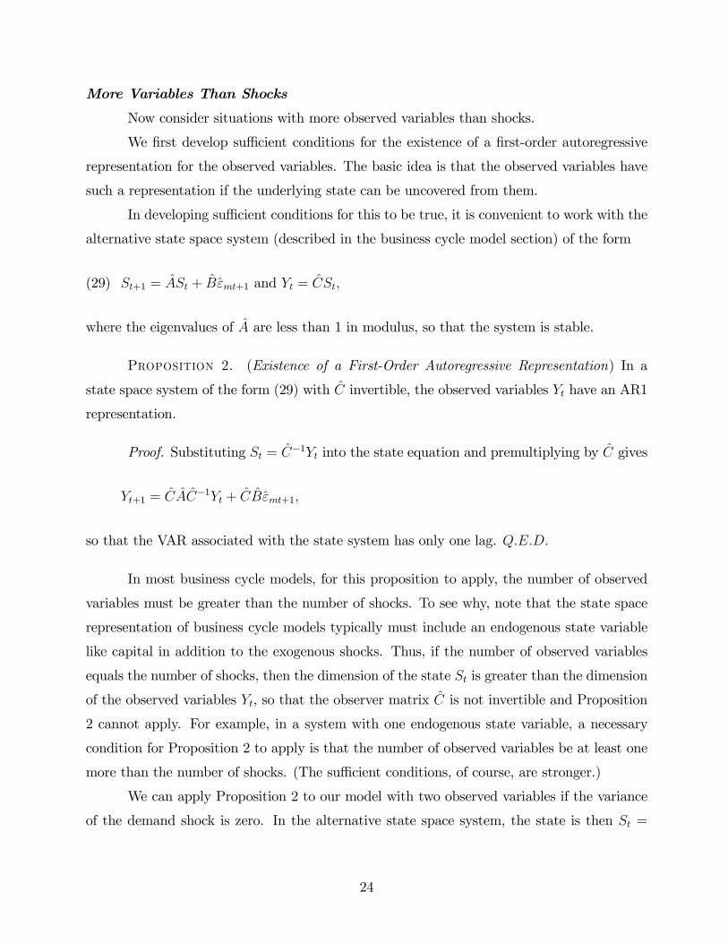
Now consider situations with more observed variables than shocks.

We first develop sufficient conditions for the existence of a first-order autoregressive

representation for the observed variables. The basic idea is that the observed variables have

such a representation if the underlying state can be uncovered from them.

In developing sufficient conditions for this to be true, it is convenient to work with the

alternative state space system (described in the business cycle model section) of the form

(29) St+1 = ASt + Bεmt+1 and Yt = CSt,

where the eigenvalues of A are less than 1 in modulus, so that the system is stable.

Proposition 2. (Existence of a First-Order Autoregressive Representation) In a

state space system of the form (29) with C invertible, the observed variables Yt have an AR1

representation.

Proof. Substituting St = C−1Yt into the state equation and premultiplying by C gives

Yt+1 = CAC−1Yt + CBεmt+1,

so that the VAR associated with the state system has only one lag. Q.E.D.

In most business cycle models, for this proposition to apply, the number of observed

variables must be greater than the number of shocks. To see why, note that the state space

representation of business cycle models typically must include an endogenous state variable

like capital in addition to the exogenous shocks. Thus, if the number of observed variables

equals the number of shocks, then the dimension of the state St is greater than the dimension

of the observed variables Yt, so that the observer matrix C is not invertible and Proposition

2 cannot apply. For example, in a system with one endogenous state variable, a necessary

condition for Proposition 2 to apply is that the number of observed variables be at least one

more than the number of shocks. (The sufficient conditions, of course, are stronger.)

We can apply Proposition 2 to our model with two observed variables if the variance

of the demand shock is zero. In the alternative state space system, the state is then St =

24

(log kt, log zt). The matrices A and B are given in the alternative state equation⎡⎣log kt+1log zt+1

⎤⎦ =⎡⎣γk −γk0 0

⎤⎦⎡⎣log ktlog zt

⎤⎦+⎡⎣0 0

0 1

⎤⎦⎡⎣ 0

log zt+1

⎤⎦and the matrix C in the alternative observer equation⎡⎣ ∆(log yt/lt)

log lt − α log lt−1

⎤⎦ =⎡⎣θ(1− a)

³1− 1

γk

´1− θ(1− a)

a³1− α

γk

´− a1−θ

⎤⎦⎡⎣log ktlog zt

⎤⎦ .As long as C is invertible, the observables have a first-order autoregressive representation.

Along with the fact that impulse responses are continuous in the parameters, Proposition

2 provides some intuition for why in our model, when the variance of the demand shock

decreases to zero, the VAR on the observed variables is increasingly well-approximated by a

VAR with one lag.

To see that having more variables than shocks is not a sufficient condition for Proposi-

tion 2 to apply, suppose that in our model with two variables, the variance of the technology

shock is zero. In the alternative state space system, the state is then St = (log kt, τ lt, τ lt−1).

Hence, the dimension of the alternative state is greater than the dimension of the observed

variables, and the state cannot be uncovered from the observed variables. Thus, Proposition

2 does not apply.

Note that a version of Proposition 2 does apply if the dimension of the observed

variables exceeds the dimension of states. In such a case, we can augment the state with

dummy variables and then apply Proposition 2.

Proposition 2 sheds light on a literature that argues that sometimes SVARs with long-

run restrictions work well. For example, Fernández-Villaverde, Rubio-Ramírez, and Sargent

(2005) show that in Fisher’s (2006) model, the population estimates from an SVAR procedure

with one lag closely approximate the model’s impulse responses. In Appendix B we show that

Fisher’s VAR system has enough observed variables so that it is a special case of Proposition

2.

25

B. Decomposition of the Impact Error: Two Biases

>From the discussion following Proposition 1, we know that if a VAR with an infinite

number of lags were to be estimated on an infinite amount of data, then the impulse responses

from the common approach would converge, in the usual sense, to the theoretical impulse

responses. This discussion implies a natural decomposition of the impact error into that due

to small-sample bias and that due to lag-truncation bias. We do this decomposition here and

find that the SVAR error is primarily due to the lag-truncation bias.

Let A0(p, T ) denote the mean of the small-sample distribution of the SVAR impulse

response when the VAR has p lags and the length of the sample is T. In practice, this mean

is approximated as the mean across a large number of simulations. Note that the above

discussion implies that A0(p = ∞, T = ∞) coincides with the model’s theoretical impulseresponse. That convergence implies that the (level of the) impact error associated with our

implementation of the common approach is

A0(p = 4, T = 180)− A0(p =∞, T =∞).

We can decompose this error into two parts:

£A0(p = 4, T = 180)− A0(p = 4, T =∞)

¤+£A0(p = 4, T =∞)− A0(p =∞, T =∞)¤ .

The term in the first brackets is the small-sample bias, the difference between the mean of

the SVAR impulse response over simulations of length 180 when the VAR has four lags and

the SVAR population impulse response when the VAR has four lags. The term in the second

brackets is the lag-truncation bias, the difference between the SVAR population impulse

response when the VAR has four lags and the model’s theoretical impulse response.

That VARs have small-sample biases has been known at least since Hurwicz (1950):

even when the true model has a VAR with four lags, the estimated coefficients are biased in

small samples.

This type of bias is small for our model: for the QDSVAR specification, it is very

small, and for the LSVAR specification, it is small compared to the lag-truncation bias. These

findings can be seen in Figures 6A and 6B which display the biases for the Galí parameters.

For each of the two specifications, the figures show the percentage difference between the

mean A0(p = 4, T = 180) and the A0(p = ∞, T = ∞), labeled small-sample mean, and the

26

percentage difference between A0(p = 4, T =∞) and A0(p =∞, T =∞), labeled population.These, again, represent the small-sample bias and the lag-truncation bias, respectively. Note

in the figures that the small-sample bias does not vary much with the relative variance of the

demand shock, so that the comparative static properties of the lag-truncation bias are very

similar to those of the impulse response error.

These findings lead us to focus on the lag-truncation bias. As we have proven, with

a sufficiently large number of lags, the lag-truncation bias becomes arbitrarily small. We

ask how many lags are needed here for the lag-truncation bias to be small with the Galí

parameters. The answer, we find, is too many.

Figure 7 displays the QDSVAR responses for lag lengths p ranging from 4 to 300.

Notice that even with 20 lags, the lag-truncation bias of the QDSVAR specification is large.

On these graphs, note that the convergence to the model’s impulse response function is not

monotonic. Finally, note that more than 200 lags are needed for the lag-truncation bias of

the QDSVAR to be small.

Figure 8 shows the impulse responses from the LSVAR for lag lengths p ranging from

4 to 100. Here, as with the QDSVAR, we see that the impulse response from the LSVAR is

a good approximation to the model’s impulse response only for an extremely large number

of lags. In practice, of course, accurately estimating VARs with so many lags is not feasible.

To understand the source of the lag-truncation bias, recall that in computing the im-

pulse responses from a VAR, we use the estimated covariance matrix Ω and the estimated sum

of the moving-average coefficients matrix C. In unreported work, we show that the primary

source of the lag-truncation bias is that the estimated matrix C is a poor approximation to

the true matrix Cm from the model.

To get some intuition for why with four lags C is a poor approximation to Cm, recall

from (4) that

(30) C =

"I −

4Xi=1

Bi

#−1

while

(31) Cm =

"I −

∞Xi=1

Bmi

#−1.

27

To develop the intuition for why the estimated sumP4

i=1Bi is a poor approximation to the

model’s sumP∞

i=1Bmi, note that Proposition 1 implies that the autoregressive coefficients

Bmi in the model decay according to the matrixM . As we have shown, the largest eigenvalue

of M is close to 1, so that the estimated sum is a poor approximation to the model’s sum.

C. Lag-Length Tests

We have argued that the main source of the error in the common SVAR procedure is

the lag-truncation bias. Here we ask whether a researcher applying the SVAR procedure and

standard methods of detecting appropriate lag lengths to data for our model would detect

the business cycle model’s need for more than four lags. We computed a variety of lag-length

tests, including the Akaike criterion, the Schwartz criterion, and a likelihood ratio test on

data generated from our model. Here we report on the results for the Galí parameters. We

find that none of these tests detects the need for more lags.

We generated from our model 1,000 sequences of length 180 for the variables used in

the two SVAR procedures. For the QDSVAR specification, we find that the Akaike criterion

selects a lag length of four or fewer in over 98.6% of the simulations and the Schwartz criterion,

in all of them. The likelihood test does not reject four lags in favor of five lags in over 92.8%

of the simulations. In Figure 9A, we graph the mean of the Akaike and Schwartz criteria for

the QDSVAR specification against the number of lags. The means of both of these criteria

are minimized at one lag.

We repeated the lag-length tests for the LSVAR specification. Now the Akaike criterion

selects a lag length of four or fewer in over 99.6% of the simulations and the Schwartz criterion,

again, in all of them. The likelihood test does not reject four lags in favor of five lags in over

94.4% of the simulations. In Figure 9B, we graph the mean of the Akaike and Schwartz

criteria for the LSVAR specification against the number of lags. The means of both of these

criteria are again minimized at one lag.

Taken together, these results suggest that with samples of roughly the same length as

U.S. data, a researcher using standard methods would not detect the need for more lags for

the VAR in either specification. At a mechanical level, the reason the Akaike and Schwartz

lag-length tests do not detect the need for more lags is simple. These tests balance the gain

in the fit of the model from adding more parameters against a fixed penalty for doing so. As

more parameters are added, the gain in the fit of the model is smaller than the penalty.

28

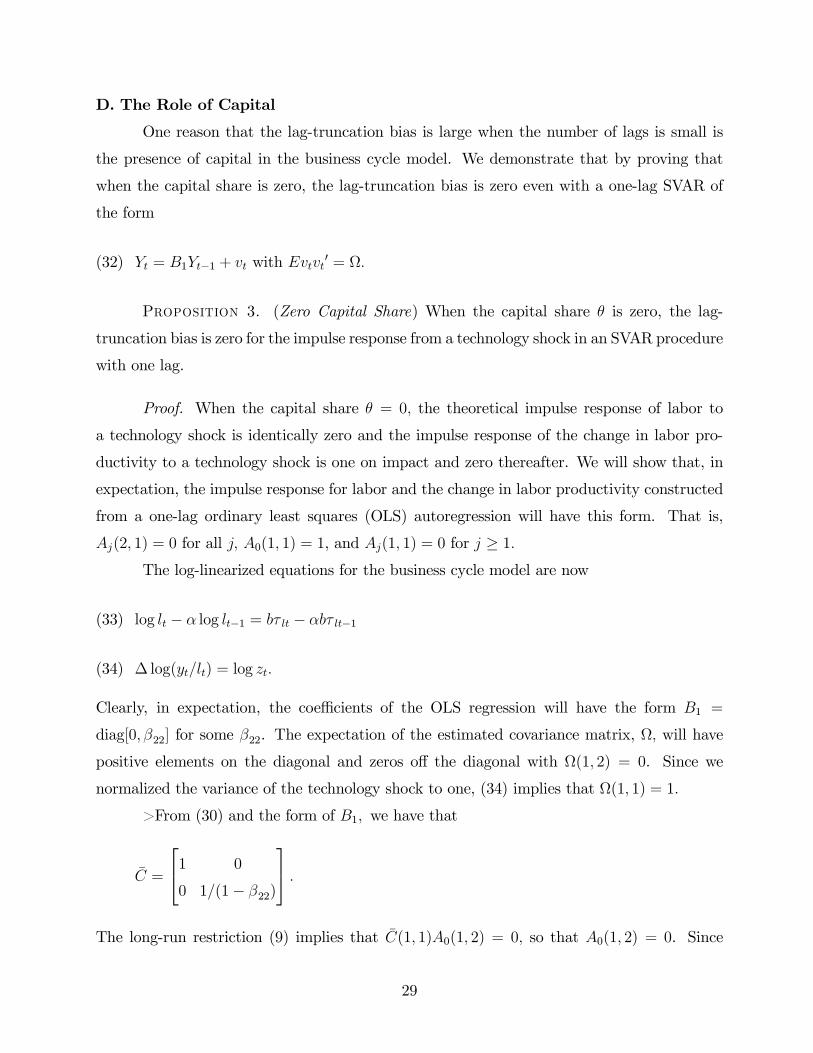
D. The Role of Capital

One reason that the lag-truncation bias is large when the number of lags is small is

the presence of capital in the business cycle model. We demonstrate that by proving that

when the capital share is zero, the lag-truncation bias is zero even with a one-lag SVAR of

the form

(32) Yt = B1Yt−1 + vt with Evtvt0 = Ω.

Proposition 3. (Zero Capital Share) When the capital share θ is zero, the lag-

truncation bias is zero for the impulse response from a technology shock in an SVAR procedure

with one lag.

Proof. When the capital share θ = 0, the theoretical impulse response of labor to

a technology shock is identically zero and the impulse response of the change in labor pro-

ductivity to a technology shock is one on impact and zero thereafter. We will show that, in

expectation, the impulse response for labor and the change in labor productivity constructed

from a one-lag ordinary least squares (OLS) autoregression will have this form. That is,

Aj(2, 1) = 0 for all j, A0(1, 1) = 1, and Aj(1, 1) = 0 for j ≥ 1.The log-linearized equations for the business cycle model are now

(33) log lt − α log lt−1 = bτ lt − αbτ lt−1

(34) ∆ log(yt/lt) = log zt.

Clearly, in expectation, the coefficients of the OLS regression will have the form B1 =

diag[0, β22] for some β22. The expectation of the estimated covariance matrix, Ω, will have

positive elements on the diagonal and zeros off the diagonal with Ω(1, 2) = 0. Since we

normalized the variance of the technology shock to one, (34) implies that Ω(1, 1) = 1.

>From (30) and the form of B1, we have that

C =

⎡⎣1 0

0 1/(1− β22)

⎤⎦ .The long-run restriction (9) implies that C(1, 1)A0(1, 2) = 0, so that A0(1, 2) = 0. Since

29

A0A00 = Ω, we know that

(35) A0(1, 1)2 +A0(1, 2)

2 = Ω(1, 1) = 1

(36) A0(1, 1)A0(2, 1) +A0(1, 2)A0(2, 2) = Ω(1, 2) = 0.

From (35) and A0(1, 2) = 0 and our sign restriction, we know that A0(1, 1) = 1. Since

A0(1, 1) 6= 0 and A0(1, 2) = 0, (36) implies that A0(2, 1) = 0. For the subsequent coefficients

Aj , recall from (7) that Aj = CjA0. From (3), Cj = Bj1, so that Cj = diag[0, y] for some y.

Hence, Aj(2, 1) = 0 and Aj(1, 1) = 0 for j ≥ 1. Q.E.D.

Note that, at least when the quasi-differencing parameter α is nonzero, observed vari-

ables do not have a first-order autoregressive representation. In particular, the lag-truncation

bias for a demand shock will not be zero.

We also experimented with increasing the depreciation rate as another way of reducing

the importance of capital. We found that when the depreciation is so high that capital

essentially depreciates completely within a year, the lag-truncation bias is close to zero.

4. Does Adding Variables and Shocks Help?So far we have focused on an SVAR with just two variables–the log difference of

labor productivity and a measure of the labor input–and two shocks–one to technology

and one to demand. In the SVAR literature, researchers often check how their results change

when they add one or more variables and shocks to the SVAR. Would such an alteration to

the SVAR we have been testing help it with our business cycle model? We find that with

additional variables and shocks, the SVAR procedure can sometimes uncover the model’s

impulse response to shocks, but only if the states are an invertible function of the observables.

Which variables should be added to the SVAR? How about some form of capital? Our

discussion of Proposition 3 suggests that one of the problems with the SVAR specification is

that it does not include such a variable. In our business cycle model, the relevant state variable

is kt = kt/Zt−1. However, since Zt−1 is not observable, we cannot include kt itself in the SVAR.

We consider instead several stationary capital-like variables: the capital/output ratio kt/yt,

the investment/output ratio xt/yt, and the growth rate of the capital stock log kt+1 − log kt.One conjecture is that including such variables might diminish the need for estimating a

large number of lags in the SVARs, so that the specifications with few lags will yield accurate

30

measures of the model’s response to a technology shock. This conjecture turns out to be, in

general, incorrect.

As we show in a separate technical appendix (Chari, Kehoe, and McGrattan 2005),

when we add the capital/output ratio or the growth rate of the capital stock to the list of vari-

ables in the VAR, we find that the model’s moving-average representation of these variables

is not invertible. In both specifications, the autoregressive coefficients decay according to the

matrix M, in a manner similar to that in Proposition 1. When we add the capital/output

ratio, one of the eigenvalues ofM is −∞, whereas when we add the growth rate of the capitalstock, one of the eigenvalues is 1. Since both specifications suffer from the type of invertibility

problems discussed by Hansen and Sargent (1991), we do not investigate them here.

So now we turn to the alternative state space representation of a three-shock model

and ask if we can find a third variable for which the SVAR specification mimics the model’s

state space representation. In the LSVAR specification, we find that if we add kt+1/yt, the

ratio of the capital stock in period t+1 to output in period t, then the SVAR representation

mimics the state space representation. In this exceptional case, the lag-truncation bias of the

LSVAR procedure is zero.

This finding does not imply, however, that adding kt+1/yt is a general prescription

for success for the SVAR procedure. For example, when we add kt+1/yt to the QDSVAR

specification, the SVAR representation does not mimic the state space representation, and

the lag-truncation bias of the SVAR procedure is not zero. More generally, across models, a

careful examination of the state space representation for each model could lead to a different

SVAR specification for each model. If so, estimating the state space representation implied

by the model directly is both safer and more transparent.

In practice, most researchers prefer using the investment/output ratio as a capital-like

variable rather than measures that use the capital stock directly because they think that the

capital stock is poorly measured. The issues of invertibility and measurement lead us to use

the investment/output ratio to capture the influence of the capital-like variable.

Let’s see what happens with this ratio included. Consider an SVAR with three vari-

ables and three shocks. The third variable is the log of the investment/output ratio xt/yt,

where xt = (1+ γ)kt+1− (1− δ)kt. Here, in addition to the growth of labor productivity and

the measure of labor, Yt includes the investment/output ratio. We let the investment tax be

31

the third shock. We assume that taxes on investment follow the autoregressive process

(37) τxt+1 = (1− ρx)τx + ρxτxt + εxmt+1,

where εxmt, together with our earlier shocks εzmt and εdmt, are jointly normal, independent of

each other, and i.i.d. over time. The standard deviation of εxmt is σx.

For this altered SVAR, Propositions 1 and 2 immediately apply. The eigenvalues of

A − BD−1C equal those of M and are given by α, (1 − δ)/(1 + gy), and 0, where gy is the

growth rate of (total) output. The analog of Corollary 1 is

Corollary 2. The eigenvalues of A−BD−1C are less than 1 if α ∈ [0, 1).

Given our parameters, the eigenvalue (1 − δ)/(1 + gy) = .98. This large eigenvalue

helps provide intuition for why an autoregression with a small number of lags is a poor

approximation to the infinite-order autoregression and, hence, (30) is a poor approximation

to (31). Interestingly, the largest eigenvalue of the decay matrixM is roughly the same in the

two- and three-variable SVARs, so that adding another variable does not seem to diminish

the need for many lags in the VAR.

We also have experimented with four-variable SVARs and four shocks. Relative to the

baseline business cycle model, we have added shocks to the tax on investment and government

consumption. In the SVAR specifications, we have added the investment/output ratio and

the consumption/output ratio as variables. Proposition 1 applies to this case, and the four

eigenvalues of the decay matrix are given by α, (1− δ)/(1 + gy), 0, and 0.

As we have noted in our discussion following Proposition 2, having more observed

variables than shocks is not a recipe for success. For a three-variable SVAR, say, Yt =

(∆ log(yt/lt), lt, xt/yt), and only two shocks, the technology shock and the labor tax shock,the three observed variables in the QDSVAR do not have a first-order autoregressive rep-

resentation. The reason is that the alternative state St = (log kt, log zt, τ lt, τ lt−1) has four

variables, so that with three observed variables, the matrix C in the observer equation is not

invertible.

Next we examine a quantitative version of our three-shock model with a three-variable

LSVARwith Yt = (∆ log(yt/lt), lt, xt/yt) and show that the lag-truncation bias and the impacterrors are large even for small variances of the investment tax shock. Figure 10 displays the

32

lag-truncation bias (labeled population), the impact error (labeled small-sample mean), and

the confidence bands for the LSVAR with four lags against the percentage of the HP-filtered

output due to the investment tax shock for ρx = .95, with the Galí parameters for the labor

tax shock. We get similar results for other values of ρx.

Figure 10 shows that the lag-truncation bias is zero when the variance of the third

shock is zero, as indicated by our earlier discussion. The figure also shows that this error

increases rapidly with the variability due to the investment tax shock. For example, the

error is over 100% if the variance of output due to the investment tax shock is 7% or more.

Interestingly, even when the variance due to the third shock is essentially zero, the impact

error is positive due to the small-sample bias. Finally, the figure shows that the SVAR’s

confidence bands are extremely wide even when the variance due to the third shock is tiny.

One might interpret Proposition 2 as suggesting that the SVAR procedure will ap-

proximately uncover the model’s impulse response as long as a relatively small number of

shocks (or factors) account for the bulk of fluctuations in the data. Figure 10 shows that this

interpretation should be treated with caution.

5. Is the Evidence Decisive?As we have seen, the QDSVAR and the LSVAR specifications do reasonably well only

when technology shocks account for virtually all of the variability in output. How likely

is that to be true? If demand shocks are usually trivial, then SVARs may be useful after

all. Here we examine five types of evidence on the relative size of technology and demand

shocks. We show that this evidence is far from decisive. Four types of evidence lead to the

conclusion that demand shocks must play a significant role in output’s variability, and one

type of evidence points to a wide range of estimates for the contribution of technology shocks.

Therefore, any claim that the data definitively imply that technology shocks account

for virtually all of the variability in output is exceptionally difficult to support. The data do

not rule out the possibility that demand shocks play a nontrivial role in output variability;

indeed, some aspects of the data suggest that they play a substantial role. If demand shocks

play a nontrivial role, then both SVAR specifications perform poorly.

In presenting this evidence, we use results both from the baseline business cycle model,

in which a labor tax is the second shock, and an investment wedge model, in which the

investment tax is the second shock. In the investment wedge model, we assume that taxes

33

on investment follow the process described in (37).

A. Evidence Based on the SVAR Central Finding

One type of evidence on the relative size of the two shocks is based on the central

result of the SVAR literature, Galí’s (1999) widely noted finding that a positive technology

shock drives down hours worked on impact. For our SVAR model to generate that finding,

technology shocks must account for only a modest fraction of output variability.

We demonstrate that in Figure 11. There we plot the mean of the SVAR impact

coefficients against the ratio of the innovation variance for both the QDSVAR (top graph)

and the LSVAR (bottom graph) specifications, fixing ρl at .95. (In the technical appendix

(Chari, Kehoe, and McGrattan 2005), we repeat this experiment for several values of ρl and

find similar results.) In the top graph of Figure 11, the upper horizontal solid line (labeled “To

reproduce Galí’s estimate”) is set so that the mean impact coefficient equals −.33, the impactcoefficient consistent with Galí’s (1999) bivariate DSVAR.8 We thus refer to the associated

parameters as the Galí parameters.

This figure can be used to indirectly infer the relative contribution of technology and

demand shocks. As we have argued above, in evaluating SVARs with long-run restrictions,

the model’s parameters should be such that the SVAR on the model’s data reproduces the

central finding of the SVAR literature: a positive technology shock drives down hours on

impact. We have investigated above what the ratio of the innovation variances must be in

order for the mean of the QDSVAR’s impact coefficient of hours to a technology shock to be

similar to Galí’s (1999) impact coefficient. As Figure 11 and Table 1 indicate, at this value

of the impact coefficient, the variance of output due to a technology shock is roughly 50% for

our baseline model.

Figure 11 shows that if demand shocks are unimportant relative to technology shocks,

then the QDSVAR impact coefficient is positive and, therefore, of the opposite sign of that

estimated by Galí. For example, if the demand shock accounts for more than 30% of the

variability in output, then the QDSVAR error is greater than 100, so that the impact coeffi-

8Galí (1999) reports that on impact, a one standard deviation technology shock leads to a −.38% changein hours. We convert this statistic to the response to a 1% technology shock, z, by dividing his statistic by thestandard deviation of the technology shock. We use Prescott’s (1986) measure of the standard deviation ofan innovation to total factor productivity σTFP to construct the standard deviation of the technology shockσz. The relationship between these standard deviations is σz = σTFP /(1− θ). Prescott measures σTFP to be.763, and our capital share is θ = .33, so that after conversion Galí’s statistic becomes −.33 (= −.38/σz).

34

cient is positive. Put differently, if demand shocks were this small, then there would be no

controversy over what happens after a technology shock and, hence, no SVAR literature to

critique.

We also conducted a similar exercise in the investment wedge model. As Table 2

shows, with this model, when the standard deviation of investment tax shocks is set so that

the QDSVAR impact coefficient mimics Gali’s coefficient, technology shocks account for 46%

of the variability in output and the error in the LSVAR impact coefficient is 188%.

B. Other SVAR Evidence

The SVAR literature also provides direct evidence on the modest relative contribution

of technology shocks to the variability in output.

Galí and Rabanal (2005), for example, use a VAR procedure on various measures

of U.S. output and employment. For their measure of the fraction of output variability

due to technology shocks, these researchers use the variance of the estimated business cycle

component of the historical series for output associated with technology shocks relative to

the sample variance of output. For their LSVAR specification, Galí and Rabanal’s point

estimates range from 3% to 37%. (For the DSVAR specification, they range from 6% to

31%.) Other SVAR studies find similar ranges.

These findings suggest that, at least for the purpose of evaluating the SVAR procedure,

models in which demand shocks do not account for the bulk of the fluctuations in output are

not interesting. Substantively, of course, as we have seen, impact errors and confidence bands

associated with the SVAR procedure are large precisely when demand shocks do account for

the bulk of the fluctuations.

C. Evidence Based on the Volatility of Hours in U.S. Data

A third type of evidence is based on the volatility of the U.S. time series hours worked.

We ask how large demand shocks must be if our business cycle model is to reproduce the

volatility of this series. One motivation for asking this question is that many of the recent

developments in business cycle theory are driven by the observation that business cycle models

with only technology shocks cannot produce anywhere near the volatility of hours in the data.

This failure is particularly marked when the technology shock has a unit root. We find that

for our model to reproduce the actual volatility of U.S. hours, demand shocks must be so

volatile that the SVAR procedure performs poorly.

35

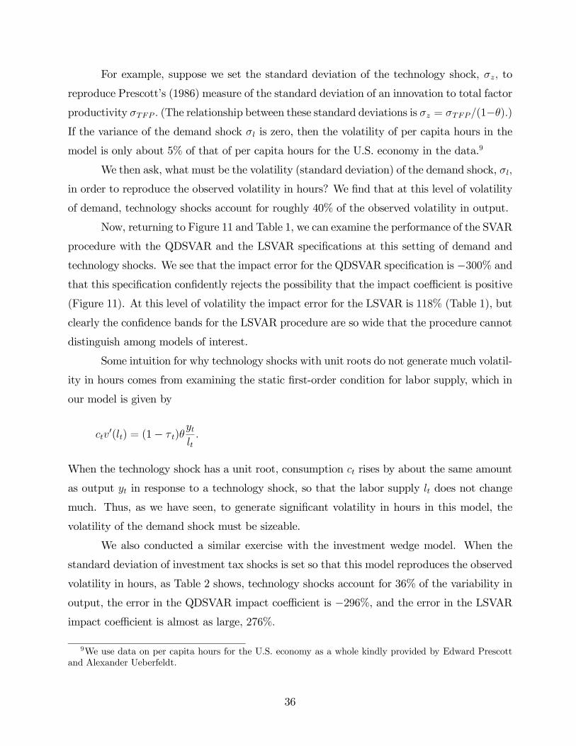
For example, suppose we set the standard deviation of the technology shock, σz, to

reproduce Prescott’s (1986) measure of the standard deviation of an innovation to total factor

productivity σTFP . (The relationship between these standard deviations is σz = σTFP/(1−θ).)If the variance of the demand shock σl is zero, then the volatility of per capita hours in the

model is only about 5% of that of per capita hours for the U.S. economy in the data.9

We then ask, what must be the volatility (standard deviation) of the demand shock, σl,

in order to reproduce the observed volatility in hours? We find that at this level of volatility

of demand, technology shocks account for roughly 40% of the observed volatility in output.

Now, returning to Figure 11 and Table 1, we can examine the performance of the SVAR

procedure with the QDSVAR and the LSVAR specifications at this setting of demand and

technology shocks. We see that the impact error for the QDSVAR specification is −300% andthat this specification confidently rejects the possibility that the impact coefficient is positive

(Figure 11). At this level of volatility the impact error for the LSVAR is 118% (Table 1), but

clearly the confidence bands for the LSVAR procedure are so wide that the procedure cannot

distinguish among models of interest.

Some intuition for why technology shocks with unit roots do not generate much volatil-

ity in hours comes from examining the static first-order condition for labor supply, which in

our model is given by

ctv0(lt) = (1− τ t)θ

ytlt.

When the technology shock has a unit root, consumption ct rises by about the same amount

as output yt in response to a technology shock, so that the labor supply lt does not change

much. Thus, as we have seen, to generate significant volatility in hours in this model, the

volatility of the demand shock must be sizeable.

We also conducted a similar exercise with the investment wedge model. When the

standard deviation of investment tax shocks is set so that this model reproduces the observed

volatility in hours, as Table 2 shows, technology shocks account for 36% of the variability in

output, the error in the QDSVAR impact coefficient is −296%, and the error in the LSVARimpact coefficient is almost as large, 276%.

9We use data on per capita hours for the U.S. economy as a whole kindly provided by Edward Prescottand Alexander Ueberfeldt.

36

D. Evidence Based on Maximum Likelihood Estimation

A fourth type of evidence on the relative sizes of the two shocks is the results of

maximum likelihood estimation. We ask what relative sizes this procedure produces for

various specifications of the observed variables. We conducted several such exercises and

found that the estimates are sensitive to the list of observed variables: their range is enormous,

and so are the impact errors of both specifications. The maximum likelihood estimates do

not support the notion that technology shocks dominate demand shocks.

In our maximum likelihood procedure, we fix all the parameters of the model except for

those of the stochastic processes. We then use the maximum likelihood procedure described

by McGrattan (1994) and Anderson et al. (1996) to estimate the parameters of the vector

AR1 process, (14) and (15), using several specifications for the observed variables, denoted

Vt. In this procedure, we write the system in a state space form with a state of the form

Xt = (log kt, log zt, τ lt, log kt−1, log zt−1, τ lt−1). The transition equation is

(38) Xt+1 = EXt + Fεmt+1,

where εmt = (0, ε0mt, 0).The observer equation is

(39) Yt = HXt.

We report on two specifications of the observer equation for both the QDSVAR and

the LSVAR. The estimates of the key parameters and some statistics of interest for the two

specifications are reported in Table 1. In the hours specification, we let the observed variables

be Yt = (∆ log yt, log lt)0. In the investment specification, we let Yt = (∆ log yt, ∆ log xt)0. In

both specifications, we impose an upper bound of .995 on the persistence parameter ρl. In

the hours specification, the variability of output due to technology is fairly large, 76%; the

impact error for the QDSVAR is −86%; and the impact error for the LSVAR is 3%. In theinvestment specification, the variability of output due to technology is more modest, 30%;

the impact error for the QDSVAR is −438%; and the impact error for the LSVAR is 190%.Clearly, the impact error for both the QDSVAR and the LSVAR depends sensitively on the

specification of observed variables.

We then asked which specification is preferable, in the sense that it leads to more

accurate estimates of the key parameters of the stochastic process. To answer this question,

37

we conducted Monte Carlo experiments for our baseline business cycle model. We set the

key parameters at ρl = .99, σl = 1%, and σz = 1%. We generated 1,000 simulations of

the same length as the actual data. For each simulation, we estimated the parameters of the

stochastic process with maximum likelihood using the specifications of the observed variables.

We imposed the same bound on ρl of .995 as in our estimation using actual data.

>From Table 3 we see that the investment specification clearly yields more accurate

estimates of the model parameters than does the hours specification. We repeated this exercise

using higher values of ρl and found that the investment specification continues to yield more

accurate estimates of the model parameters. These findings lead us to prefer the investment

specification for estimating the model’s parameters.

Clearly, the variability of output due to technology shocks associated with the max-

imum likelihood estimates is sensitive to the variables included in the observer equation,

especially investment. The reason for this sensitivity is that a stripped-down model like ours

cannot mimic well all of the comovements in U.S. data, so that it matters what features of

the data the researcher is primarily interested in. Full information methods like maximum

likelihood turn out to be sensitive to details such as which variables are included in the es-

timation. Our Monte Carlo experiments lead us to prefer the investment specification. And

this specification leads to a large impact error for the LSVAR.

We also used maximum likelihood to estimate the hours and the investment specifica-

tions for the investment wedge model. Here again we imposed an upper bound of .995 on the

autoregressive parameter ρx. Table 2 shows that under both specifications, technology shocks

account for about three-quarters of the variability in output. The associated impact error is

about −70% for the QDSVAR and nearly 60% for the LSVAR. Given the size of the impact

error, maximum likelihood estimates do not support the view that demand shocks are trivial.

E. Evidence from the Growth Model Literature

Finally, we consider one more type of evidence on the relative size of the two shocks:

the business cycle literature based on the growth model. This literature contains a wide range

of estimates for the fraction of output variability due to technology shocks.

The studies differ in their data and in the details of the procedure they use to compute

estimates, but all attempt to measure a broadly similar conceptual object. And they get very

different results. For example:

38

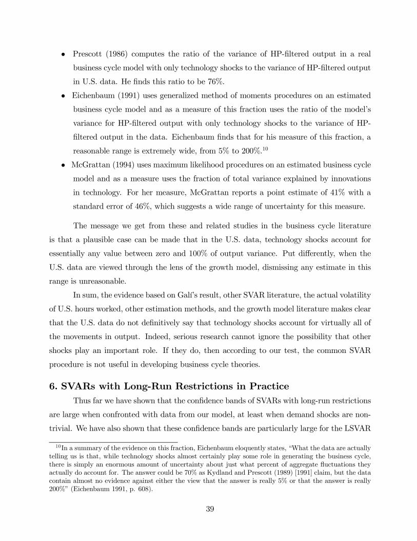
• Prescott (1986) computes the ratio of the variance of HP-filtered output in a real

business cycle model with only technology shocks to the variance of HP-filtered output

in U.S. data. He finds this ratio to be 76%.

• Eichenbaum (1991) uses generalized method of moments procedures on an estimated

business cycle model and as a measure of this fraction uses the ratio of the model’s

variance for HP-filtered output with only technology shocks to the variance of HP-

filtered output in the data. Eichenbaum finds that for his measure of this fraction, a

reasonable range is extremely wide, from 5% to 200%.10

• McGrattan (1994) uses maximum likelihood procedures on an estimated business cycle

model and as a measure uses the fraction of total variance explained by innovations

in technology. For her measure, McGrattan reports a point estimate of 41% with a

standard error of 46%, which suggests a wide range of uncertainty for this measure.

The message we get from these and related studies in the business cycle literature

is that a plausible case can be made that in the U.S. data, technology shocks account for

essentially any value between zero and 100% of output variance. Put differently, when the

U.S. data are viewed through the lens of the growth model, dismissing any estimate in this

range is unreasonable.

In sum, the evidence based on Galí’s result, other SVAR literature, the actual volatility

of U.S. hours worked, other estimation methods, and the growth model literature makes clear

that the U.S. data do not definitively say that technology shocks account for virtually all of

the movements in output. Indeed, serious research cannot ignore the possibility that other

shocks play an important role. If they do, then according to our test, the common SVAR

procedure is not useful in developing business cycle theories.

6. SVARs with Long-Run Restrictions in PracticeThus far we have shown that the confidence bands of SVARs with long-run restrictions

are large when confronted with data from our model, at least when demand shocks are non-

trivial. We have also shown that these confidence bands are particularly large for the LSVAR

10In a summary of the evidence on this fraction, Eichenbaum eloquently states, “What the data are actuallytelling us is that, while technology shocks almost certainly play some role in generating the business cycle,there is simply an enormous amount of uncertainty about just what percent of aggregate fluctuations theyactually do account for. The answer could be 70% as Kydland and Prescott (1989) [1991] claim, but the datacontain almost no evidence against either the view that the answer is really 5% or that the answer is really200%” (Eichenbaum 1991, p. 608).

39

compared to the QDSVAR. Here we conduct a different test: We examine the performance

of the two SVAR specifications when confronted with actual U.S. data.

We find that whatever the data set or subsample, the QDSVAR specification produces

basically the same results. That is not true for the LSVAR, however. For that specification,

small conceptual differences in the underlying data which lead to small differences in cyclical

properties lead to large differences in the impulse responses. The impulse responses of that

specification are also very different across subsamples. These findings using actual data are

consistent with our findings using data generated from our model, and they buttress a result of

the rest of our work here, that the LSVAR specification is of questionable value in developing

business cycle theory.

These findings come from applying the SVAR procedure to three popular U.S. data sets

used in the SVAR literature: those of Francis and Ramey (2005b); Christiano, Eichenbaum,

and Vigfusson (2003); and Galí and Rabanal (2005). The three data sets cover somewhat

different time periods but use conceptually similar measures of productivity and hours worked.

In Figure 12A, we plot the measures of hours used in the three studies. The figure suggests

that the cyclical fluctuations of the three series are virtually identical, but that the series

show some differences in trend behavior in the first part of the sample. In Figure 12B, we

plot the HP-filtered cyclical component of these three series and see that they are indeed

virtually identical.

The QDSVAR performs similarly with all three data sets. With all of them, a positive

technology shock leads to a fall in hours on impact. Thus, here we focus mainly on the impulse

responses and the associated confidence bands obtained by running the LSVAR specification

with four lags on these data sets. We find that the LSVAR specification yields sharply differing

results for the three data sets. With this specification, on impact a positive technology shock

leads to a fall in hours in one, a rise in hours in another, and basically no change in the

third. These large differences in results across similar data sets are likely to be connected to

our finding about the wide range of LSVAR impulse responses across simulations from our

model.

The fall in hours is predicted by the LSVAR when we use the data that Francis and

Ramey (2005b) constructed to estimate an LSVAR for the period 1948:1—2002:4. Their

measure of productivity is the U.S. Bureau of Labor Statistics (BLS) series “Index of Output

per Hour, Business.” Francis and Ramey construct a new measure of hours by adjusting the

40

BLS series “Index of Hours in Business” for government employment and for demographic

changes. Figure 12C illustrates that with these data, an innovation resulting in a 1% increase

in total factor productivity leads to a persistent decline in hours. On impact, the decline is

1.9%, a value significantly different from zero at the 5% level.

The LSVAR predicts a rise in hours when we follow Christiano, Eichenbaum, and

Vigfusson (2003), who use the DRI Basic Economics database to estimate an LSVAR for the

period 1948:1—2001:4. Their measure of productivity is business labor productivity (LBOUT),

and their measure of hours is business hours divided by the civilian population over the age

of 16 (LBMN and P16 ). Figure 12D shows that with these data, a positive technology shock

leads to a persistent rise in hours. On impact a 1% increase in total factor productivity

results in a .5% increase in hours. Notice that while the impact coefficient is not significantly

different from zero, the response coefficients are significant from lag 3 onward.11

Finally, the LSVAR predicts no change in hours on impact from the technology shock

when we follow Galí and Rabanal (2005) and use data for 1948:1—2002:4. Their measure

of productivity is business labor productivity, constructed as the ratio of nonfarm business

sector output to hours worked by all persons in the nonfarm business sector. For hours, Galí

and Rabanal use the ratio of nonfarm hours to the civilian population over the age of 16. The

source is the Haver USECON database, and their measures of output, hours, and population

are LXNFO, LXNFH, and LNN, respectively. Figure 12E indicates that with these data, a

positive technology shock leads to a persistent but statistically insignificant rise in hours. On

impact, the rise is essentially zero, and that is not significantly different from zero at the 5%

level.

These sharply contrasting results have led researchers in the SVAR literature to draw

sharply contrasting inferences. Francis and Ramey (2005b) argue that their evidence shows

that real business cycle models are dead. Christiano, Eichenbaum, and Vigfusson (2003)

maintain that the models are alive and well. Galí and Rabanal (2005) assert that the ex-

isting results are inconclusive; they prefer the alternative DSVAR specification, which, they

argue, also shows that real business cycle models are dead. Interestingly, these studies use

11Christiano, Eichenbaum, and Vigfusson (2003) use an instrumental variables procedure that Shapiro andWatson (1988) proposed, rather than our OLS procedure, and they compute Bayesian confidence intervalsrather than our bootstrapped confidence intervals. Comparing our Figure 10D with Figure 2 in their paperreveals that the mean impulse response is similar, but that they have much tighter confidence bands than wedo.

41

similar conceptual measures of productivity, and two of them (Christiano, Eichenbaum, and

Vigfusson 2003 and Galí and Rabanal 2005) use similar conceptual measures of hours as well.

A recent literature has argued that the LSVAR impulse responses are unstable in the

sense that they differ across subsamples (Fernald 2005, Gambetti 2005, and the references in

both). We find some evidence of instability as well. For example, with the Francis and Ramey

(2005b) data set, the impact coefficient over the whole sample is −1.80 with a confidenceband of (−2.31,−.48), whereas over the period 1970:1—2002:4, it is quite different: .19 witha confidence band of (−.55, .57).

The sensitivity of the LSVAR results to seemingly minor differences in measuring

productivity and hours and across subsamples raises serious doubts about the reliability of

the LSVAR procedure for drawing inferences about underlying models.

7. Related LiteratureOur critique of the SVAR approach adds to nearly 30 years of other critiques of this

approach. Previous critiques can be broadly divided into those based on invertibility prob-

lems, those using economic models as tests, those of circular specification searches, and those

based on deep inference problems when the parameter spaces are infinite-dimensional.

In a pair of insightful but often-neglected papers, Hansen and Sargent (1980, 1991)

point out that invertibility problems may plague the type of Box-Jenkins methods that un-

derlie the SVAR literature. (See also Fernández-Villaverde, Rubio-Ramírez, and Sargent

2005.) Hansen and Sargent show that interesting economic models could have noninvertible

moving-average representations and that this noninvertibility could cause problems for simple

statistical procedures that do not use enough economic theory.

Lippi and Reichlin (1993), along the lines of Hansen and Sargent (1991), analyze how

invertibility problems could lead to mistaken inferences in the Blanchard-Quah procedure.

Blanchard and Quah (1993) argue that although such problems may arise for some examples,

they typically have not arisen in most applied models. Blanchard and Quah also argue that

even when such problems do arise, the resulting inference mistakes may not be quantitatively

large. Our critique is different from the Hansen-Sargent invertibility critique because our

specifications do not suffer from invertibility problems.

Cooley and Dwyer (1998) lucidly critique the SVAR procedure using economic models

as tests in a manner broadly similar to ours. One important difference between our work

42

and theirs, however, is that they mainly focus on models that violate the key assumptions of

the SVAR approach either by not having a unit root in the technology shock or by having

correlated shocks. We focus on models that satisfy the key assumptions of the SVAR approach

and show through a series of propositions that even then the SVAR approach may fail to

uncover the models’ impulse responses. Another difference is that we focus on the central

conclusion of the recent SVAR literature, that technology shocks lead to a fall in hours,

whereas Cooley and Dwyer focus on a variety of other issues. (For work similar in spirit to

that of Cooley and Dwyer, see also McGrattan 2005.)

Erceg, Guerrieri, and Gust (2004) also test the SVAR procedure using economic mod-

els. In contrast to our focus on theoretical propositions about population moments, their

main focus is on small-sample bias in SVARs, and they conclude that the small-sample bias

problem in models is modest. Most important, they conclude that “overall, Galí’s method-

ology appears to offer a fruitful approach to uncovering the effects of technology shocks”(p.

4). We conclude the opposite.

Uhlig (2005) criticizes what he sees as the circularity of searching over specifications

until a certain pattern is found and then arguing that the data show that finding such a

pattern is strong evidence for a certain theory.

Faust and Leeper (1997) discuss inference problems in infinite-dimensional VARs that

underlie the SVAR approach. They argue that “unless strong restrictions are applied, con-

ventional inferences regarding impulse responses will be badly biased in all sample sizes” (p.

345). They show that under a long-run identifying scheme, any test of the magnitude of an

impulse response coefficient has a significance level greater than or equal to its power.

Faust and Leeper’s results build on a pair of seminal papers by Sims (1971, 1972),

who shows that in infinite-dimensional spaces, unless severe restrictions are imposed on the

parameters, standard methods cannot be used to make asymptotically valid confidence state-

ments.

8. ConclusionSimple data analysis techniques that reliably point toward quantitatively promising

models can be highly useful in applied economic analysis. The SVAR literature seems to

hold out hope that SVAR is such a technique. The common, long-run restriction branch of

this literature has attracted a great deal of interest because it claims that the procedure can

43

accurately distinguish between promising classes of models without having to take a stand

on the details of other shocks, besides minimal features such as orthogonality.

Our study concludes that this claim is true in principle: if researchers had long enough

data sets, then the SVAR procedure would accurately identify the model’s impulse response

with only minimal assumptions on the details of the other shocks. In practice, however,

the claim is not true. When demand shocks play a substantial role, SVARs with long-

run restrictions yield accurate estimates of the impulse responses only if the sum of the

autoregressive coefficients in the VAR is close to that of those in the model. With the typical

small number of lags in the VAR, these sums are not close in a model like ours. Since the

length of available data sets requires that the VAR have a small number of lags, SVARs with

long-run restrictions work poorly.

The SVAR claim is also true in principle if the number of observables is sufficiently

greater than the number of shocks, so that the observables in the VAR can be inverted to

uncover the state of the model. Our examples suggest, however, that this finding must be

interpreted with caution.

We emphasize that our analysis is not a critique of SVARs in general. It is also not

a critique of SVARs with long-run restrictions. It is only a critique of SVARs with long-run

restrictions that use the common approach of comparing inappropriate objects, empirical and

theoretical impulse responses. As Sims (1989) has argued and Cogley and Nason (1995) have

shown, SVARs that instead compare logically comparable objects may be useful in developing

business cycle theories.

Elsewhere (in Chari, Kehoe, and McGrattan, 2007), we have argued for the usefulness

of another approach to developing business cycle theory: business cycle accounting. This

approach has the same goal as the SVAR approach–to quickly shed light on which of a class

of models is promising–but business cycle accounting suffers from fewer shortcomings.

44

ReferencesAltig, David; Christiano, Lawrence; Eichenbaum, Martin; and Linde, Jesper. 2005.

Firm-Specific Capital, Nominal Rigidities and the Business Cycle. Working Paper 11034,

Cambridge: National Bureau of Economic Research.

Anderson, Evan W.; Hansen, Lars Peter; McGrattan, Ellen R.; and Sargent, Thomas

J. 1996. Mechanics of Forming and Estimating Dynamic Linear Economies. In Handbook of

Computational Economics, vol. 1, edited by Hans M. Amman, David A. Kendrick, and John

Rust, 171—252. Amsterdam: North-Holland/Elsevier.

Bencivenga, Valerie R. 1992. An Econometric Study of Hours and Output Variation

with Preference Shocks. International Economic Review 33 (2): 449—71.

Benhabib, Jess; Rogerson, Richard; and Wright, Randall. 1991. Homework in Macro-

economics: Household Production and Aggregate Fluctuations. Journal of Political Economy

99 (6): 1166—87.

Bernanke, Ben S.; Gertler, Mark; and Gilchrist, Simon. 1999. The Financial Ac-

celerator in a Quantitative Business Cycle Framework. In Handbook of Macroeconomics,

vol. 1C, edited by John B. Taylor and Michael Woodford, 1341—93. Amsterdam: North-

Holland/Elsevier.

Blanchard, Olivier Jean, and Quah, Danny. 1989. The Dynamic Effects of Aggregate

Demand and Supply Disturbances. American Economic Review 79 (4): 655—73.

. 1993. The Dynamic Effects of Aggregate Demand and Supply Distur-

bances: Reply. American Economic Review 83 (3): 653—58.

Braun, R. Anton. 1994. Tax Disturbances and Real Economic Activity in the Postwar

United States. Journal of Monetary Economics 33 (3): 441—62.

Chari, V. V.; Kehoe, Patrick J.; and McGrattan, Ellen R. 2005. Technical Appendix

to “A Critique of Structural VARs Using Real Business Cycle Theory.” Manuscript, Federal

Reserve Bank of Minneapolis.

. 2007. Business Cycle Accounting. Econometrica 75 (3): 781—836.

Christiano, Lawrence J.; Eichenbaum, Martin; and Evans, Charles L. 2005. Nominal

Rigidities and the Dynamic Effects of a Shock to Monetary Policy. Journal of Political

Economy 113 (1): 1—45.

Christiano, Lawrence J.; Eichenbaum, Martin; and Vigfusson, Robert. 2003. What

Happens After a Technology Shock? Working Paper 9819, National Bureau of Economic

45

Research.

Cogley, Timothy, and Nason, James M. 1995. Output Dynamics in Real-Business-

Cycle Models. American Economic Review 85 (3): 492—511.

Cooley, Thomas F., and Dwyer, Mark. 1998. Business Cycle Analysis without Much

Theory: A Look at Structural VARs. Journal of Econometrics 83 (1—2): 57—88.

Cooley, Thomas F., and Hansen, Gary D. 1989. The Inflation Tax in a Real Business

Cycle Model. American Economic Review 79 (4): 733—48.

Eichenbaum, Martin. 1991. Real Business-Cycle Theory: Wisdom or Whimsy? Jour-

nal of Economic Dynamics and Control 15 (4): 607—26.

Erceg, Christopher J.; Guerrieri, Luca; and Gust, Christopher. 2004. Can Long-

Run Restrictions Identify Technology Shocks? International Finance Discussion Papers 792,

Board of Governors of the Federal Reserve System.

Faust, Jon, and Leeper, Eric M. 1997. When Do Long-Run Identifying Restrictions

Give Reliable Results? Journal of Business and Economic Statistics 15 (3): 345—53.

Fernald, John. 2005. Trend Breaks, Long-Run Restrictions, and the Contractionary

Effects of Technology Improvements. Working Paper 2005-21, Federal Reserve Bank of San

Francisco.

Fernández-Villaverde, Jesús; Rubio-Ramírez, Juan F.; and Sargent, Thomas J. 2005.

A, B, C’s, (and D’s) for Understanding VARs. Technical Working Paper 0308, National

Bureau of Economic Research.

Fisher, Jonas D. M. 2006. The Dynamic Effects of Neutral and Investment-Specific

Technology Shocks. Journal of Political Economy 114 (3): 413—51.

Francis, Neville, and Ramey, Valerie A. 2005a. Is the Technology-Driven Real Business

Cycle Hypothesis Dead? Shocks and Aggregate Fluctuations Revisited. Journal of Monetary

Economics 52 (8): 1379—99.

. 2005b. Measures of Per-Capita Hours and Their Implications for the

Technology-Hours Debate. Working Paper 11694, National Bureau of Economic Research.

Galí, Jordi. 1999. Technology, Employment, and the Business Cycle: Do Technology

Shocks Explain Aggregate Fluctuations? American Economic Review 89 (1): 249—71.

Galí, Jordi; López-Salido, David J.; and Vallés, Javier. 2003. Technology Shocks

and Monetary Policy: Assessing the Fed’s Performance. Journal of Monetary Economics 50:

723—43.

46

Galí, Jordi, and Rabanal, Pau. 2005. Technology Shocks and Aggregate Fluctuations:

How Well Does the RBC Model Fit Postwar U.S. Data? NBER Macroeconomics Annual

2004, vol. 19, edited by Mark Gertler and Kenneth Rogoff, 225—88. Cambridge, Mass.: MIT

Press.

Gambetti, Luca. 2005. Technology Shocks and the Response of Hours Worked: Time-

Varying Dynamics Matter. Manuscript, Universitat Pompeu Fabra, Barcelona, Spain.

Greenwood, Jeremy, and Hercowitz, Zvi. 1991. The Allocation of Capital and Time

over the Business Cycle. Journal of Political Economy 99 (6): 1188—214.

Hall, Robert E. 1997. Macroeconomic Fluctuations and the Allocation of Time. Jour-

nal of Labor Economics 15 (1, Part 2): S223—50.

Hansen, Gary D. 1985. Indivisible Labor and the Business Cycle. Journal of Monetary

Economics 16 (3): 309—27.

Hansen, Lars Peter, and Sargent, Thomas. 1980. Formulating and Estimating Dy-

namic Linear Rational Expectations Models. Journal of Economic Dynamics and Control 2

(1): 7—46.

. 1991. Two Difficulties in Interpreting Vector Autoregressions. InRational

Expectations Econometrics, 77—119. Underground Classics in Economics. Boulder: Westview

Press.

Hurwicz, Leonid. 1950. Least Squares Bias in Time Series. In Statistical Inference in

Dynamic Economic Models, edited by Tjalling C. Koopmans, 365—83. New York: Wiley.

Kydland, Finn E., and Prescott, Edward C. 1982. Time to Build and Aggregate

Fluctuations. Econometrica 50 (6): 1345—70.

. 1991. Hours of Employment Variation in Business Cycle Theory. Eco-

nomic Theory 1 (1): 61—81.

Lippi, Marco, and Reichlin, Lucrezia. 1993. The Dynamic Effects of Aggregate De-

mand and Supply Disturbances: Comment. American Economic Review 83 (3): 644—52.

Marcet, Albert. 2005. Overdifferencing VARs is OK. Manuscript, Universitat Pompeu

Fabra.

McGrattan, Ellen R. 1994. The Macroeconomic Effects of Distortionary Taxation.

Journal of Monetary Economics 33 (3): 573—601.

. 2005. Comment on Galí and Rabanal’s “Technology Shocks and Aggre-

gate Fluctuations: How Well Does the RBC Model Fit Postwar U.S. Data?” NBER Macro-

47

economics Annual 2004, vol. 19, edited by Mark Gertler and Kenneth Rogoff, 289—308.

Cambridge, Mass.: MIT Press.

Prescott, Edward C. 1986. Theory Ahead of Business Cycle Measurement. Federal

Reserve Bank of Minneapolis Quarterly Review. 10 (4, Fall), 9—22.

Quah, Danny. 1990. Permanent and Transitory Movements in Labor Income: An

Explanation for “Excess Smoothness” in Consumption. Journal of Political Economy 98 (3):

449—75.

Rotemberg, Julio J., and Woodford, Michael. 1992. Oligopolistic Pricing and the

Effects of Aggregate Demand on Economic Activity. Journal of Political Economy 100 (6):

1153—1207.

Shapiro, Matthew D., and Watson, Mark W. 1988. Sources of Business Cycle Fluc-

tuations. NBER Macroeconomics Annual 1988, vol. 3, edited by Stanley Fischer, 111—48.

Cambridge, Mass.: MIT Press.

Sims, Christopher A. 1971. Distributed Lag Estimation When the Parameter Space

Is Explicitly Infinite-Dimensional. Annals of Mathematical Statistics 42: 1622—36.

. 1972. The Role of Approximate Prior Restrictions in Distributed Lag

Estimation. Journal of the American Statistical Association 67 (337): 169—75.

. 1989. Models and Their Uses. American Journal of Agricultural Eco-

nomics 71 (2): 489—94.

Stockman, Alan C., and Tesar, Linda L. 1995. Tastes and Technology in a Two-

Country Model of the Business Cycle: Explaining International Comovements. American

Economic Review 85 (1): 168—85.

Uhlig, Harald. 2005. What Are the Effects of Monetary Policy on Output? Results

from an Agnostic Identification Procedure. Journal of Monetary Economics 52 (2): 381—419.

48

Appendix AIdentification Using Long-Run Restrictions

Here we show that the two key assumptions of an SVAR along with the sign restric-

tion identify the impulse responses of both variables in the VAR to a technology shock as

summarized by the first columns of the matrices Ai.

Consider the system of four (independent) equations made up of (8) and (9) in the

four unknowns of A0. These can be written as

(40) A0(1, 1)2 +A0(1, 2)

2 = ω11

(41) A0(1, 1)A0(2, 1) +A0(1, 2)A0(2, 2) = ω12

(42) A0(2, 1)2 +A0(2, 2)

2 = ω22

(43) C(1, 1)A0(1, 2) + C(1, 2)A0(2, 2) = 0.

First suppose that C(1, 1) is not equal to zero. Then we can manipulate equations (40)—(43)

to obtain one equation in A0(2, 2):

fA0(2, 2)2 +

£ω11 − f 2A0(2, 2)

2¤1/2 £

ω22 − A0(2, 2)2¤1/2

= ω12,

where f = −C(1, 2)/C(1, 1). This equation is quadratic in A0(2, 2)2 and can be solved to

obtain

(44) A0(2, 2)2 =

ω11ω22 − ω212ω11 − 2fω12 + f2ω22

,

while the other elements of A0 are given by

A0(1, 2) = −fA0(2, 2)

A0(1, 1)2 = ω11 − f 2A0(2, 2)

2

A0(2, 1)2 = ω22 − A0(2, 2)

2.

We then need to use (11), the sign restriction,

(45) C(1, 1)A0(1, 1) + C(1, 2)A0(2, 1) > 0,

to pick the relevant roots of the quadratics. Using the definition of f, we can rewrite equation

49

(41) as

(46) A0(1, 1)A0(2, 1) + fA0(2, 2)2 = ω12

and use that to rewrite (45) as

(47) C(1, 1)A0(1, 1) + C(1, 2)£ω12 − fA0(2, 2)

2¤/A0(1, 1) > 0.

Combined with (44), this equation pins down the sign of A0(1, 1). Equation (46) pins down

the sign of A0(2, 1). Thus, we have shown that as long as C(1, 1) is not equal to zero, the

first column of A0 is identified. Clearly, the first column of Ai = CiA0 is also identified for

all i ≥ 1.When C(1, 1) equals zero but C(1, 2) does not, equation (43) implies that A0(2, 2) =

0, and a similar argument can be used to show that the first column of Ai is identified for

i ≥ 0.Note that much of the literature does not explicitly mention that a necessary condition

for the four conditions (40)—(43) to pin down the first column of A0 is that at least one of

C(1, 1) or C(1, 2) be nonzero. If both are zero, then (43) places no restrictions on A0, and

clearly the first column of A0 varies in many solutions to the three equations (40)—(42) in

the four unknowns of A0. A condition that is sufficient to imply that at least one of C(1, 1)

or C(1, 2) is nonzero is (10), so that a technology shock has a nonzero long-run effect on the

level of labor productivity.

50

Appendix BA Special Case of Proposition 2

Here we show that Fisher’s (2006) model is not subject to our critique because it has

a first-order autoregressive representation. We first lay out Fisher’s (2006) model along the

lines of Fernández-Villaverde, Rubio-Ramírez, and Sargent (2005) and then transform it to

relate it to our baseline model. Finally, we work out the transformed model’s state space

representation and show that it falls under the domain of our Proposition 2. In this sense, it

is not surprising that the common approach works well in Fisher’s model.

In Fisher’s model, the planner maximizes expected utility E0P∞

t=0 βt[log c∗t +ψ log(1−

lt)] over per capita consumption c∗t and per capita labor lt, subject to the resource constraint

(48) Vtc∗t + xt = Atk

θt lt

1−θ

and the law of motion for capital

(49) kt+1 = (1− δ)kt + Vtxt,

where xt is investment, At is a neutral technology shock that follows the unit root process,

(50) logAt+1 = μa + logAt + log at+1,

and Vt is an investment-specific technology shock that follows the unit root process of the

form

(51) logVt+1 = μv + log Vt + log vt+1.

Note that Vt is also the price of the investment good relative to output goods, and output ytis Atk

αt l1−at .

We can transform Fisher’s model to be similar to that of our baseline model. Let

ct = Vtc∗t and substitute (49) into (48) to give

(52) ct + kt+1 − (1− δ)ktxt = VtAtkθt lt

1−θ(≡ yt).

Letting Z1−αt = VtAt and noting that in the objective function log c∗t = log Vt + log ct, this

model is equivalent to the baseline model (with an irrelevant additive constant in the objective

function). The log-linearized decision rules for Fisher’s economy thus are (16)—(18) without

the demand shock. Note that care must be taken not to confuse output in Fisher’s model

51

with output in the equivalent baseline model: in Fisher’s model, again, output yt is Atkαt l1−at ,

so that Vtyt = VtAtkθt lt

1−θ = kθt (Ztlt)1−θ = Ztyt; therefore,

(53) ∆ log yt = ∆ log yt +

µ1

1− θ

¶log at +

µθ

1− θ

¶log vt.

Fisher assumes that the observed variables are the growth rate of labor productivity

∆ log(yt/lt), the labor input lt, and the change in the log of the relative price of investment

∆ log Vt, which equals log vt. We can use the equivalent baseline model to work out the state

space system for our model. Note from (53) that to recover log yt we need to record both log atand log vt separately in the state. The state of the system is Xt = (log kt, log at, log vt)

0. The

state equation Xt+1 = AXt + Bεmt+1 is⎡⎢⎣log kt+1log at+1

log vt+1

⎤⎥⎦ =⎡⎢⎣γk −γk/(1− θ) −γk/(1− θ)

0 0 0

0 0 0

⎤⎥⎦⎡⎢⎣log ktlog at

log vt

⎤⎥⎦+⎡⎢⎣ 0

log at+1

log vt+1

⎤⎥⎦ .The observer equation Yt = CXt is⎡⎢⎣∆ log(yt/lt)log lt

log vt

⎤⎥⎦ =⎡⎢⎣θ(1− a)(1− 1

γk) 1−θ(1−a)

1−θθa1−θ

a − a1−θ − a

1−θ0 0 1

⎤⎥⎦⎡⎢⎣log ktlog at

log vt

⎤⎥⎦ .Since C is invertible, Proposition 2 applies, and Fisher’s model has a first-order autoregressive

representation.

52

Table 1. Parameter Estimates and Statistics of Interest for the Model with Taxes on Labor

Parameter Estimates Statistics of Interesta

Impact Error

Evidence ρl σz σl %var(y) QDSVAR LSVAR

Galı VAR response .950 .0114 .0073 50 −220 76(−344,−79) (−230,245)

Hours volatility .950 .0114 .0088 40 −300 118(−448,−132) (−252,322)

Maximum likelihoodb

Hours specification .995 .0114 .0050 76 −86 3(.0093) (.0006) (.0005) (−171,−5) (−219,123)

Investment specification .942 .0178 .0173 30 −438 190(.0076) (.0016) (.0013) (−616,−226) (−270,442)

a The first statistic is the variance of output due to the technology shock, reported as a percent. The last two are themean impact errors for the QDSVAR and LSVAR specifications. The values in parentheses are means of the upper andlower means of 95 % confidence bands across 1,000 applications of the VAR procedure.

b For the maximum likelihood parameter estimates, the values in parentheses are standard errors. The hours specificationuses observations on output and labor, and the investment specification uses observations on output and investment.

Table 2. Parameter Estimates and Statistics of Interest for the Model with Taxes on Investment

Parameter Estimates Statistics of Interesta

Impact Error

Evidence ρx σz σx %var(y) QDSVAR LSVAR

Galı VAR response .950 .0114 .0143 46 −221 188(−368,−67) (−120,327)

Hours volatility .950 .0114 .0175 36 −296 276(−471,−108) (−88,431)

Maximum likelihoodb

Hours specification .995 .0116 .0096 76 −73 57(.0071) (.0006) (.0010) (−158,7) (−145,137)

Investment specification .995 .0088 .0071 77 −69 53(.0078) (.0004) (.0007) (−152,8) (−144,130)

a The first statistic is the variance of output due to the technology shock, reported as a percent. The last two are themean impact errors for the QDSVAR and LSVAR specifications. The values in parentheses are means of the upper andlower means of 95 % confidence bands across 1,000 applications of the VAR procedure.

b For the maximum likelihood parameter estimates, the values in parentheses are standard errors. The hours specificationuses observations on output and labor, and the investment specification uses observations on output and investment.

Table 3. Monte Carlo Analysis of Maximum Likelihood Estimation

for Two Sets of Observables in the Model with Taxes on Labor

Hours Specificationa Investment Specificationb

Estimates ρl σz σl ρl σz σl

True estimates .990 .0100 .0100 .990 .0100 .0100

Monte Carlo estimatesMean .980 .0101 .0096 .990 .0100 .0100

Maximum .995 .0121 .0119 .992 .0117 .0128

Minimum .838 .0083 .0074 .986 .0084 .0070

% Standard deviation 1.83 .053 .084 .076 .053 .083

a The hours specification uses observations on output and labor.b The investment specification uses observations on output and investment.

! "#$ %'&( () +*,- . /"# 02143 /0 #. 5

Quarter Following Shock

Res

pons

eto

1%T

FP

Sho

ck

Res

pons

eto

1%T

echn

olog

yIn

nova

tion

0 4 8 12 16 20 24 28 32 36 40 44 48 52 56 600

0.1

0.2

0.3

0.4

0.5

0

0.1

0.2

0.3

*. ) 22 %) / 3( 0.

Mean Error in the Impact Coefficient of Hours From 1,000 Applications ofthe Four-Lag SVAR Procedures Applied to Model Simulations of Length 180,

Varying Innovations of the Shock Processes

Ratio of Innovation Variances (σl2/σz

2)

Per

cent

Err

or

0 0.2 0.4 0.6 0.8 1-500

-450

-400

-350

-300

-250

-200

-150

-100

-50

0

50

100

150

200

250ρ=.95ρ=.9ρ=.99ρ=.995

ρ=.995ρ=.99

ρ=.95ρ=.9

LSVAR Results

QDSVAR Results

*

*. ) 2 *" *"# % ) / 3 2 0.

Mean Error in the Impact Coefficient of Hours (solid line) and 95%Confidence Bands (dashed lines) From 1,000 Applications of the Four-Lag

QDSVAR Procedure with ρl = .95 Applied to Model Simulations of Length 180,

Varying the Variance of Output Due to Technology

HP-filtered Output Variance Due to Technology (%)

Per

cent

Err

or

-700

-600

-500

-400

-300

-200

-100

0

100

100 4067 2950 34

*. ) 2 *" *"# %) / 3( 0.

Mean Error in the Impact Coefficient of Hours (solid line) and 95%Confidence Bands (dashed lines) From 1,000 Applications of the Four-Lag

LSVAR Procedure with ρl = .95 Applied to Model Simulations of Length 180,

Varying the Variance of Output Due to Technology

HP-filtered Output Variance Due to Technology (%)

Per

cent

Err

or

-300

-200

-100

0

100

200

300

400

500

100 67 50 40 34 29

*

3( & ) 02* *" "0(% * #*2*)2

Histogram of Impact Coefficient of Hours and 95% Bounds on ImpulseResponses From 1,000 Applications of the Four-Lag QDSVAR Procedure

to Model Simulations of Length 180

Response to 1% TFP Shock

Pro

babi

lity

ofR

espo

nse

onIm

pact

-2 -1 0 10

0.01

0.02

0.03

0.04

0.05

0.06

Quarter Following Shock

Res

pons

eto

1%T

FP

Sho

ck

0 2 4 6 8 10 12-1.5

-1

-0.5

0

0.5

97.5% of SVAR Results Below

97.5% of SVAR Results Above

Model Impulse Response

3 "0! *" *"0(% * 0*2*)2

Mean Impulse Response of Hours (solid line) and Mean of 95% BootstrappedConfidence Bands (dashed lines) Averaged Across 1,000 Applications

of the Four-Lag QDSVAR Procedure to Model Simulations of Length 180

Quarter Following Shock

Res

pons

eto

1%T

FP

Sho

ck

Res

pons

eto

1%T

echn

olog

yIn

nova

tion

0 1 2 3 4 5 6 7 8 9 10 11 12-1.5

-1

-0.5

0

0.5

-1

-0.5

0

*

3 & !) #2* *" "# % (* #*2* )

Histogram of Impact Coefficient of Hours and 95% Bounds on ImpulseResponses From 1,000 Applications of the Four-Lag QDSVAR Procedure

to Model Simulations of Length 180

Response to 1% TFP Shock

Pro

babi

lity

ofR

espo

nse

onIm

pact

-1 0 1 20

0.01

0.02

0.03

0.04

0.05

0.06

Quarter Following Shock

Res

pons

eto

1%T

FP

Sho

ck

0 2 4 6 8 10 12-1

0

1

2

97.5% of SVAR Results Below

97.5% of SVAR Results Above

Model Impulse Response

3 "# *" *"0 % (* #*2*)2

Mean Impulse Response of Hours (solid line) and Mean of 95% BootstrappedConfidence Bands (dashed lines) Averaged Across 1,000 Applications

of the Four-Lag QDSVAR Procedure to Model Simulations of Length 180

Quarter Following Shock

Res

pons

eto

1%T

FP

Sho

ck

Res

pons

eto

1%T

echn

olog

yIn

nova

tion

0 1 2 3 4 5 6 7 8 9 10 11 12

-0.5

0

0.5

1

1.5

-0.5

0

0.5

1

*

*. ) 2 *" *"# % ) / 3 2 0.

Mean Error in the Impact Coefficient of Hours (solid line) and 95%Confidence Bands (dashed lines) From 1,000 Applications of the Four-Lag

QDSVAR Procedure with ρl = .95 Applied to Model Simulationsof Length 180 and Population Errors (dotted line),

Varying the Variance of Output Due to Technology

HP-filtered Output Variance Due to Technology (%)

Per

cent

Err

or

-700

-600

-500

-400

-300

-200

-100

0

100

100 4067 2950 34

Population

SmallSample Mean

*. ) 2 *" *"# %) / 3( 0.

Mean Error in the Impact Coefficient of Hours (solid line) and 95%Confidence Bands (dashed lines) From 1,000 Applications of the Four-Lag

LSVAR Procedure with ρl = .95 Applied to Model Simulationsof Length 180 and Population Errors (dotted line),

Varying the Variance of Output Due to Technology

HP-filtered Output Variance Due to Technology (%)

Per

cent

Err

or

-300

-200

-100

0

100

200

300

400

500

100 67 50 40 34 29

Population

Small Sample Mean

+ *" 3 *)2 " ! "# % &(

Using Galı Parameters and Varying Lag Length p in QDSVAR Procedure

Quarter Following Shock

Res

pons

eto

1%T

FP

Sho

ck

Res

pons

eto

1%T

echn

olog

yIn

nova

tion

0 4 8 12 16 20 24 28 32 36 40 44 48 52 56 60-0.75

-0.5

-0.25

0

0.25

0.5

0.75

-0.5

-0.25

0

0.25

0.5

p=4

p=10

p=20

p=30

p=50

Model Impulse Response

QDSVAR Impulse Responses (dashed lines)

Quarter Following Shock

Res

pons

eto

1%T

FP

Sho

ck

Res

pons

eto

1%T

echn

olog

yIn

nova

tion

0 4 8 12 16 20 24 28 32 36 40 44 48 52 56 60-0.5

-0.25

0

0.25

0.5

0.75

-0.25

0

0.25

0.5p=100

p=50

Model Impulse Response

QDSVAR Impulse Responses (dashed lines)p=200

p=300

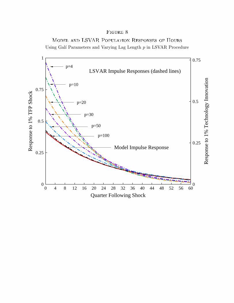
*" 3( *)2 " "0! %'&(

Using Galı Parameters and Varying Lag Length p in LSVAR Procedure

Quarter Following Shock

Res

pons

eto

1%T

FP

Sho

ck

Res

pons

eto

1%T

echn

olog

yIn

nova

tion

0 4 8 12 16 20 24 28 32 36 40 44 48 52 56 600

0.25

0.5

0.75

1

0

0.25

0.5

0.75p=4

p=10

p=20

p=30

p=50

Model Impulse Response

LSVAR Impulse Responses (dashed lines)

p=100

*

* "#) /,- !) ) / * ) *&( *# ( % %"#.

Information Criteria for Tests of 1,000 Model Simulations of Length 180

Number of Lags

Info

rmat

ion

Cri

teri

on

1 2 3 4 5 6 7 8-18.5

-18

-17.5

-17

Akaike

Schwartz

* "0) / ,- !) ) / * ) *&( ( "

Information Criteria for Tests of 1,000 Model Simulations of Length 180

Number of Lags

Info

rmat

ion

Cri

teri

on

1 2 3 4 5 6 7 8-18.5

-18

-17.5

-17

Akaike

Schwartz

*. ) 2 % ) / , / * * 3 #.

Mean Error in the Impact Coefficient of Hours (solid line)and 95% Confidence Bands (dashed lines) From 1,000 Applications ofthe Four-Lag, Three-Variable LSVAR Procedure Applied to Model

Simulations of Length 180 and Population Errors (dotted line),

Varying Innovations of the Shock Processes

HP-filtered Output Variance Due to Investment Tax (%)

Per

cent

Err

or

-300

-200

-100

0

100

200

300

400

0 7 13 19 24 28

Population

Small Sample Mean

""# *)2 "* *"#. -*)2 1 * *" 30&( Demand Shock Innovation is Varied to Reproduce Galı’s (1999) Estimate for

the Impulse Response of Hours to a Technology Shock and to Generatethe Same Variance of Hours as in U.S. Data

HP-filtered Output Variance Due to Technology (%)

Per

cent

Err

or

-700

-600

-500

-400

-300

-200

-100

0

100

100 4067 2950 34

To reproduce Gali’s estimate

To reproduce variance of U.S. hours

ConfidenceBands forParametersReproducingHours Variance

ConfidenceBandsfor "Gali"Parameters

QDSVAR Results

HP-filtered Output Variance Due to Technology (%)

Per

cent

Err

or

-300

-200

-100

0

100

200

300

400

500

100 67 50 40 34 29

ConfidenceBandsfor "Gali"Parameters

ConfidenceBands forParametersReproducingHours Variance

LSVAR Results

*

, / 3 (% $) / & * ) * "

Hou

rsP

erC

apita

(200

0:1

=1)

1950 1955 1960 1965 1970 1975 1980 1985 1990 1995 20000.7

0.8

0.9

1

1.1

1.2

Christiano et al. (2003)

Gali and Rabanal (2004)

Francis and Ramey (2004)

, /& % ) 3 (% $) / &( * )* "

HP

-Filt

ered

Log

Hou

rsP

erC

apita

(%)

1950 1955 1960 1965 1970 1975 1980 1985 1990 1995 2000-7

-6

-5

-4

-3

-2

-1

0

1

2

3

4

5

6

7

Christiano et al. (2003)

Gali and Rabanal (2004)

Francis and Ramey (2004)

.

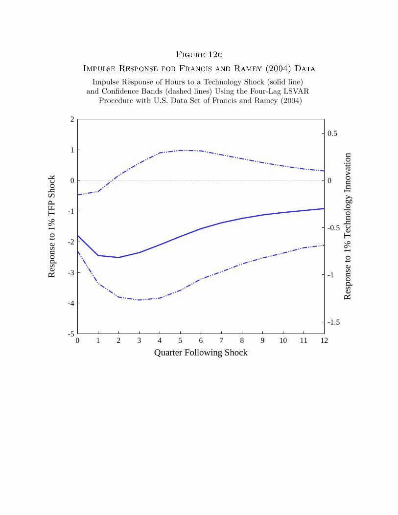
!$ "# % 2*"#. *" -* 1 *)*Impulse Response of Hours to a Technology Shock (solid line)

and Confidence Bands (dashed lines) Using the Four-Lag LSVARProcedure with U.S. Data Set of Francis and Ramey (2004)

Quarter Following Shock

Res

pons

eto

1%T

FP

Sho

ck

Res

pons

eto

1%T

echn

olog

yIn

nova

tion

0 1 2 3 4 5 6 7 8 9 10 11 12-5

-4

-3

-2

-1

0

1

2

-1.5

-1

-0.5

0

0.5

"#% / )2 *"# )$* *)*Impulse Response of Hours to a Technology Shock (solid line)

and Confidence Bands (dashed lines) Using the Four-Lag LSVAR Procedurewith U.S. Data Set of Christiano, Eichenbaum, and Vigfusson (2003)

Quarter Following Shock

Res

pons

eto

1%T

FP

Sho

ck

Res

pons

eto

1%T

echn

olog

yIn

nova

tion

0 1 2 3 4 5 6 7 8 9 10 11 12-5

-4

-3

-2

-1

0

1

2

-4

-3

-2

-1

0

1

! "# % * *" * *"* *)*Impulse Response of Hours to a Technology Shock (solid line)

and Confidence Bands (dashed lines) Using the Four-Lag LSVARProcedure with U.S. Data Set of Galı and Rabanal (2004)

Quarter Following Shock

Res

pons

eto

1%T

FP

Sho

ck

Res

pons

eto

1%T

echn

olog

yIn

nova

tion

0 1 2 3 4 5 6 7 8 9 10 11 12-5

-4

-3

-2

-1

0

1

2

-4

-3

-2

-1

0

1