are sunspots learnable? an experimental investigation in a

Are Sunspots Learnable? An ExperimentalInvestigation in a Simple Macroeconomic

Model

Jasmina Arifovic, George Evans and Olena Kostyshyna∗

August 20, 2019

Abstract

We conduct experiments with human subjects in a model witha positive production externality in which productivity is a nonde-creasing function of the average level of employment of other firms.The model has three steady states and a sunspot equilibrium thatfluctuates between the high and low steady states. Steady states arepayoff ranked: low values give lower profits than higher values. Weinvestigate whether subjects can learn a sunspot equilibrium. We ob-serve coordination on the extrinsic announcements in our experimentaleconomies. Cases of apparent convergence to the low and high steadystates are also observed.

JEL Categories: D83, G20Keywords: sunspots, learning, experiments with human subjects

∗Arifovic: Simon Fraser University, Department of Economics, 8888 University Drive,Burnaby, BC, V5A 1S6, Canada, [email protected]. Evans: University of Oregon, 1285 Uni-versity of Oregon, Eugene, OR, USA and University of St. Andrews, [email protected]: Bank of Canada, 234 Wellington Street Ottawa, ON, K1A 0G9, Canada,[email protected]. The views expressed in this paper are those of the authors. Noresponsibility for them should be attributed to the Bank of Canada. We would like tothank Heng Sok and Brian Merlob for helpful research assistance.

1 Introduction

In this paper, we present an experimental study of a model with multiplepayoff-rankable equilibria, including a sunspot equilibrium. The objectiveof this work is to explore whether subjects can coordinate on a sunspotequilibrium and under what circumstances such coordination arises.1

The possibility of multiple rational expectations equilibria (REE) is acentral issue in macroeconomics, raising the question of coordination andforcefully emphasizing the importance of expectations. In models with mul-tiple REE the equilibria typically include stationary sunspot equilibria (SSE)solutions, in which agents’ actions are conditioned on an extraneous randomvariable (Cass and Shell (1983)). This phenomenon can be found, for ex-ample, in overlapping-generations models of money, real business cycle-typemodels with non-convexities, New Keynesian models, endogenous growthmodels, and monetary search models. SSEs provide an interpretation of eco-nomic fluctuations as at least in part due to self-fulfilling changes in householdand firm expectations.

A question of considerable interest in macroeconomics is whether agentscan coordinate on SSEs. For example, Farmer (1999) and Clarida et al.(2000) have argued that SSEs may provide an explanation for business cyclefluctuations. Sunspot-driven fluctuations are more plausible in models inwhich SSEs are stable under adaptive learning. This possibility has beendemonstrated by Woodford (1990), Evans and Honkapohja (1994), Evans etal. (1998), Honkapohja and Mitra (2004), Evans et al. (2007), Shea (2013),McGough, Meng and Xue (2013), as well as in numerous other papers.

The potential importance of SSEs continues to generate interest. Forexample, in the context of multiple steady states due to the interest-ratezero lower bound, stressed by Benhabib, Schmidt-Grohe and Uribe (2001),the possible relevance to the Great Recession of the existence of associatedSSEs has been emphasized by Mertens and Ravn (2014). In a new generation

1Experimental studies of models with multiple equilibria have been done in differentenvironments, including overlapping generations models with money (Marimon and Sunder(1993, 1994, 1995), Lim et al (1994), Arifovic (1995, 1996), simultaneous games (Cooperet al. (1990, 1992))), effort coordination games (van Huyck et al. (1990)), optimal growthmodels with nonconvex production technology (Lei and Noussair (2007)), and bank runs(Garratt and Keister (2009), Schotter and Yorulmazer (2009)), Corbae and Duffy (2008),Arifovic et al. (2012)). Duffy (2016) and Arifovic and Duffy (2018) provide surveys of thisliterature.

1

of bubbles models, SSEs have recently been suggested as a source of assetprice volatility – see Gali (2014), Farmer (2015) and Miao, Shen and Wang(2018).

Given this background, although there is of course important related lit-erature discussed below, there has been relatively little research on SSEs inexperimental macro settings. Our aim, therefore, is to determine whether itis possible for subjects in an experimental setting to coordinate on an SSEwithin a simple and transparent economy. The sunspot equilibria we considerare in the spirit of macroeconomic models that obtain cyclical fluctuationsin settings in which multiple equilibria arise through strategic complemen-tarities, externalities or monopolistic competition. Examples include thecoordination failure models of Cooper and John (1988), the ”animal spirits”model of Howitt and McAfee (1982) based on transactions externalities, andthe multiplicities and sunspot equilibria found in non-convex real businesscycle and endogenous growth models when positive production externalitiesor monopolistic competition are present, as in Benhabib and Farmer (1994)or Evans et al. (1998).

Because in experiments it is crucial to keep the setting simple, we developa stripped-down, essentially static, framework in which a positive productionexternality leads to the existence of multiple steady states and sunspot equi-libria. We also ensure that the decision the subjects need to make each periodis simple and transparent: to forecast aggregate employment. Although theframework is very simple, this makes it possible to study whether agents cancoordinate on a sunspot equilibrium in which there are economic fluctuationsof the type found in the macroeconomic literature just cited.

The model has three steady states. In the language of the macro learn-ing literature, the low-employment and high-employment steady states areE-stable (and thus stable under adaptive learning rules), while the middlesteady state is not E-stable. There also exists an E-stable sunspot equilib-rium on which we concentrate in our experiments. This sunspot equilibriuminvolves fluctuations between values near the two E-stable steady states, i.ebetween low and high steady states. These two steady states are payoffranked: the high-employment steady state has higher profits than the low-employment steady state does. This feature presents an additional challengefor coordination on a sunspot equilibrium because it implies switching fromhigh-payoff to low-payoff outcomes.

The payoff rankability of the certainty equilibria motivates two differentexperimental treatments. In the first, the subjects’ payoff is based on prof-

2

its, which presents the challenge discussed above. In the second treatment,the subjects’ payoff is based on the forecasting accuracy of their forecasts(forecast squared error), and thus the two certainty equilibria are not payoff-ranked in this case. These two treatments allow us to address question ofwhether it is easier to coordinate on sunspot equilibria if they yield the samepayoffs as certainty equilibria.

Our motivation for using two treatments with different payoffs based onprofits and forecast squared error is also based on the observation aboutaccuracy of inflation expectations of firms and consumers relative to the ac-curacy of inflation expectations of professional forecasters. Although thesestylized facts relate to inflation expectations, we believe that the underlyinglink to the optimization function of these agents is relevant to our under-standing of expectations about employment in our experiments. Based onthe firm survey in New Zealand, Coibion et al. (2018) document that in-flation expectations of firm managers are higher than those of professionalforecasters and exhibit more disagreement than those of professional fore-casters. Ehrmann et al. (2015) show that household inflation expectationsin Michigan Survey of Consumers are above those of professional forecasters.Coibion et al. (2018) argue that inaccuracy in firms forecasts could be at-tributed to the inattention linked to the characteristics of the firms such asduration until the next price change, slope of the profit function and shareof exports in their sales. In other words, firms do not pay attention to thedynamics in aggregate inflation because it is not directly linked to their de-cision making which determines their payoffs – profits. Similar reasons weresuggested to explain bias in consumers inflation expectations – they careabout inflation for their own consumption bundle, not aggregate level. Pro-fessional forecasters, on the other hand, care directly about the accuracy oftheir forecasts, and, therefore, their forecasts are more accurate than thoseof firms or consumers. In our experiments, we implement two treatmentswith different payoffs to capture different optimization functions – profits forfirms and forecast squared error for professional forecasters. Our hypothesisis that forecasts are more accurate in the treatment with payoff based on theforecast squared error than forecasts in the treatment with payoff based onthe profits. Our findings are consistent with this hypothesis.

The main result of our experiments is that subjects can coordinate onsunspot announcements in both treatments. We also observe coordination onhigh- and low-employment steady states where subjects disregarded sunspotannouncements. While the experiments show frequent examples of coordi-

3

nation on the sunspot announcements in both treatments, in the treatmentswith forecasting accuracy, the subjects’ forecasts and outcomes are closer tothe equilibria corresponding to the announcement, i.e. the coordination ismore accurate (consistent with the hypothesis outlined above). We shouldnote that less accurate forecasts in our profit treatment can be attributedpartly to the flatness of the profit function, consistent with the finding inCoibion et al. (2018) that firms with with steeper profit function makesmaller forecast errors.

The paper is organized as follows. In section 2 we describe related lit-erature. In section 3, we describe the model. In section 4, we present thedesign of the experiments. Section 5 describes the results of the experiments,followed by section 6 which presents the discussion of adaptive learning inthe experiments. Section 7 concludes the paper.

2 Related literature

There are several related papers in the experimental literature that havelooked for sunspot equilibria in different settings. Marimon et al. (1993)perform an experimental study based on the overlapping generations modelwith money. For an appropriate specification of preferences, this model canhave multiple regular perfect foresight cycles and sunspots.2 In their set-up the model has a unique steady-state equilibrium and a two-period cycleequilibrium (which can be viewed as a perfect foresight sunspot). Marimonet al. (1993) find that while the presence of extrinsic shocks (sunspots) is notsufficient in itself to generate cyclic patterns in behavior, cyclic behavior isobserved when agents are trained to experience it together with a sunspot atthe beginning of the experiment. During training periods, the cyclic behavioris achieved by a real shock to the number of agents in a generation thatamounts to varying endowments; this shock is not observable by the subjects.The change in the number of agents is accompanied by a sunspot - a blinkingsquare of a corresponding color on the computer screen. The number ofagents in a generation is kept fixed after the training period, but the coloredsquare continues to appear on the screens during the input stage and duringthe display of the results. The display of history is also color-coded. Marimonet al. (1993) find that the price fluctuations are smaller during the experimentthan those during the training periods, but that the price fluctuations persist.

2See, for example Azariadis and Guesnerie (1986).

4

Thus there appears to be coordination on a cyclic equilibrium, though it isdifficult to tell, given the length of the experiments, how long this cyclicbehavior would continue. The cyclic behavior tends to trail off towards theend, and thus it is not clear that the SSEs are durable.

Duffy and Fisher (2005) study sunspot equilibria in a microeconomic set-ting in which heterogeneity of agents, both buyers and sellers, plays a centralrole, and motivates trades. They consider two mechanisms that have differ-ent information flows: the closed-book call market and double auction. Intheir set-up, the marginal valuations of buyers and marginal costs of sell-ers depend on the median price, and thus the payoffs of agents depend onthe actual price realized in the market. This feature turns the set-up into acoordination game, with two equilibria, but by design the two equilibria arenot Pareto rankable: some subjects are better off in one equilibrium, whereasother subjects are better off in the other equilibrium. Duffy and Fisher (2005)find that subjects can coordinate on a sunspot equilibrium based on a publicannouncement, though this result is sensitive to semantics, i.e. the wordingof the announcements, and institutions: sunspot equilibria are observed inall sessions with call markets, but in less than half of the sessions with doubleauction.

Fehr et al. (2018) study a two-player coordination game with multipleequilibria: players pick a number between zero and one hundred, and the pay-offs are determined as the squared deviations from the other player’s choice.All equilibria have the same payoff, but choosing 50 is a risk-dominant equi-librium. Fehr et al. (2018) use public and/or private signals of differentprecision and study experimentally how they affect which equilibrium sub-jects coordinate on3. Their sunspots are semantically salient (they are thenumbers just like the strategies) and they do not have training periods whichdistinguishes this paper from Marimon et al. (1993), Duffy and Fisher (2005)and ours. They find that sunspot equilibria arise endogenously in case of pub-lic signals that are easy to aggregate. They also observe sunspot-like behaviorin case of highly correlated private signals. When both public and privatesignals are provided, full coordination on public signal is disturbed as somesubjects condition their decisions on private signals. In our setup, we have

3The global games literature has shown that the existence of multiple equilibria, incoordination-type games, is sensitive to the presence of private and public signals (forexample, Heinemann et al. (2004)). These signals can in effect operate as sunspots.

5

only public announcements, and our sunspot announcements are less seman-tically salient (”Low/high employment is forecast this period”) than in Fehret al. (2018) as the announcement does not specify the values of low/highemployment. In our model sunspot equilibrium is payoff-dominated by thehigh-employment equilibrium, while in Fehr et al. (2018) sunspot equilibriado not present welfare losses.

Beugnot et al. (2012) show that in a coordination game with two strate-gies with payoff-ranked equilibria the subjects coordinate on the payoff-dominant equilibrium in the treatment without sunspots. The introductionof sunspots disrupts the coordination on the payoff-dominant equilibriumand leads to off-equilibrium outcomes (’dis-coordination’). However, sub-jects never coordinate on the payoff-dominated equilibrium4. This studyhas one feature in common with our paper – payoff-rankability of certaintyequilibria; however, this study is based on a normal form game with twostrategies, while ours is based on a macroeconomic model with a continuumof strategies. In addition, coordination on a sunspot is not observed in theirexperiment.

There are also experimental studies of correlated equilibrium, a conceptthat is related to sunspot equilibrium. For example, Duffy and Feltovich(2010) study the game of Chicken with private third-party recommendationsand show that subjects follow the third-party recommendations if they arederived from a correlated equilibrium which is payoff-enhancing relative toNash equilibria. While related, the concept of private recommendations inthe context of correlated equilibrium in their study is different from publicsunspot announcements in ours. In our paper, the signal is publicly an-nounced and informs all subjects about the forecast that is randomly gener-ated. This is different from private recommendations of strategies to subjects.Furthermore, while in Duffy and Feltovich (2010) subjects only coordinateon correlated equilibrium that is payoff-enhancing relative to Nash equilib-ria, our subjects are able to coordinate on the sunspot equilibrium which ispayoff-dominated by the high-employment equilibrium.

The focus of our paper is different, and motivated instead by the macroliterature. We look at a simple macro set-up with a positive production exter-nality and multiple steady states. In this setting there exist SSEs, and only

4Previous experimental work without sunspots has shown convergence to payoff-dominated equilibria in both normal form games (for example, Cooper et al. (1990),Van Huyck et al. (1990)) and optimal growth model with increasing returns (Lei andNoussair (2007)).

6

a subset of these SSEs can be locally stable under adaptive learning rules.We are interested in whether, in this context, adaptively stable SSEs canbe reached and sustained experimentally in the lab. In line with the macroliterature, in which it is plausible that agents may not have complete knowl-edge of the full economic structure, we provide qualitative but incompletequantitative information to subjects of the specification of the economy.

Our experiments are also related to the experimental studies of expecta-tions formation. In these studies, subjects also do not know the underlyingstructure of the economy and need to form expectations of endogenous vari-ables using observed past realizations in the economy. For the surveys ofthis macro experimental literature see Duffy (2016) and Arifovic and Duffy(2018).

Within the general literature, our work is closest to Marimon et al. (1993)and Duffy and Fisher (2005), both of which study experimentally whetherthe equilibrium selection can be driven by extraneous public announcements.Like Marimon et al. (1993), we use a macroeconomic setting to generatesunspots, but in contrast to their framework, which looks at SSEs near cyclesin a neighborhood of the indeterminate steady state, in particular at SSEsnear a 2-period cycle, we look at SSEs near a pair of distinct steady states.Duffy and Fisher (2005) also look at SSEs near distinct equilibria, but inour setting the steady states are Pareto rankable. Also we do not requireheterogeneity of agent types, and thus the sunspot equilibria that we examinehave the interpretation of switches between high and low levels of aggregateoutput, resulting from waves of optimism or pessimism driven by extraneouspublic announcements.

3 Model

3.1 Description of the economy

We use a simple, stylized macroeconomic set-up in which production exter-nalities can generate multiple steady states and SSEs. Our framework ischaracterized by the contemporaneous production externality in which pro-ductivity of a firm is increased, over a range, by higher activity in otherfirms.5

5Our set-up is closely related to the “Increasing Social Returns” overlapping generationsmodel described on pp. 72-81 in Evans and Honkapohja (1995). To keep the framework

7

In period t, each firm hires workers, nt, to produce output, yt using theproduction function

(1) yt = ψt√nt,

where ψt indexes productivity. Profit for the firm is computed as outputminus labor costs. The cost of a unit of labor is wage w, and thus the firmmaximizes profit

(2) Πt = ψt√nt − wnt,

The level of productivity ψt depends on the average level of employmentacross all other firms (not including firm’s own employment)6. We will callaverage employment of other firms Nt. The firm decides on employment,nt, before knowing productivity, ψt, because it does not know the averageemployment of other firms, Nt, when its decision is made. A firm is moreproductive when other firms are operating at a high level of employment.7

Specifically, productivity, ψt, depends on the average employment of otherfirms, Nt, as follows8:

ψt = 2.5 when Nt ≤ 11.5

ψt = 2.5 + (Nt − 11.5) when 11.5 < Nt < 13(3)

ψt = 4 when 13 ≤ Nt

This model can be thought of as a very simple and stylized macroeconomicmodel, with a single consumption good, no capital or other means of saving,

as simple as possible, for laboratory experiments, we use a version that eliminates thedynamic optimization problem required in overlapping generations set-ups, and insteadfocuses entirely on the contemporaneous production externality.

6Another alternative would be to make ψt depend on the average level of employmentof all firms. Neither implementation matters in a rational expectations equilibrium (REE)(under competitive assumptions) but they can affect the behavior of the experimentaleconomy as will be discussed later.

7As emphasized by Farmer (1999) in the context of RBC models, perfect competitionwith positive production externalities is formally equivalent to increasing returns to scaleproduction combined with monopolistic competition; for the laboratory model we employa simple version of the production externality used in Evans and Honkapohja (1995).

8Lei and Noussair (2007) study an environment similar to ours. The productivity intheir model depends on the aggregate level of capital: if aggregate capital is above thethreshold, productivity is high; if aggregate capital is below the threshold, the productivityis low. They find that experimental economies can get into poverty traps with low levelsof capital and output.

8

and in which household utility is such that labor supply is infinitely elasticat wage w.9 Firms are owned by households and profits are distributed asdividends back to the households each period. Note that, because we have arepeated static equilibrium model, the household problem is trivial: supplythe labor demanded by firms at wage w and consume all income, generatedby wages and dividends. In the experiments we therefore focus solely on thefirm problem within this setting.

3.2 Equilibria

For this economy, profits are maximized when firms choose:

(4) n =

(ψ

2w

)2

Depending on the parameters there are (generically) one or three perfectforesight steady states. Within each of the three steady states, all firmshire the same quantity of labor and produce the same level of output. Forproductivity function (3) and with wages w = 0.5, this model has 3 steadystates: nL = 6.25 (“low-level”), nM = 12.54 and nH = 16 (“high-level”).

When there are three steady states, stationary sunspot equilibria (SSE)exist between any pair of steady states. For example, in the experiments werandomly generate announcements of “high” and “low” forecasted employ-ment. Letting At ∈ {L,H} denote the announcement at time t, where L rep-resents the announcement “Low employment is forecasted this period” andH denotes the announcement “High employment is forecasted this period”,there exists an SSE nt = nL if At = L and nt = nH if At = H. Other SSEsalso exist, including those switching between other pairs of steady states orbetween all three steady states, as well as the three steady states themselvesin which employment is independent of the announcement.10

Changes in the wage w, as well as changes in employment subsidies ortaxes that alter the “effective” wage rate, can bifurcate the system. (Wage

9It would be straightforward to generalize the model to allow for less than fully elasticlabor supply, as is done in Evans and Honkapohja (1995).

10Equilibria or SSEs can be constructed that depend on any observable, e.g. equilibriacan be constructed that switch between steady states values depending on calendar timeor on the past history of aggregate employment. These equilibria can be viewed as limitingSSE. There also exists an SSE in which nt = nL if At = H and nt = nH if At = L.

9

subsidies or taxes are assumed offset by lump-sum taxes or subsidies, respec-tively so that the combined effect is revenue neutral).

When w = 1 only the “low-level” steady state exists, and when w = 0.2only the “high-level” steady-state exists. There do not exist SSEs when theeffective wage is such that only a single interior steady state exists. In thisstudy, we concentrate on the issue of coordination on SSE, and so we usew = 0.5.

We now take up the issue of which equilibria are stable under simpleadaptive learning rules that have been widely studied in the macro learningliterature.

3.3 Temporary equilibrium framework and E-stability

Sunspot-driven fluctuations are more plausible in models in which SSEs arestable under adaptive learning (Woodford (1990), Evans and Honkapohja(1994), Evans et al. (1998), and Evans et al. (2007)). In our setting onlya subset of the existing SSEs can be locally stable under adaptive learningrules. In this section, we establish which SSE is adaptively stable, and weconcentrate on it in our experiments.

The optimal choice of n in equation (4) depends on the firm’s expectationsof ψ. As ψ depends on the average employment of other firms, Nt (equation3), the optimal choice of n equivalently depends on the firm’s expectation ofNt.

If we now drop rational expectations and also the assumption of homo-geneous expectations, then the model equations are as follows. In period t,

firm i chooses its employment level as: nit = (ψe,it

2w)2 where the superscripts

e, i denote the expectations of agent i.Average employment of other firms for firm i is given by

(5) N it =

∑j 6=i n

jt

K − 1

where there are K firms, and the actual current productivity level of firm iis given by ψ(N i

t ) according to equation (3). The output of firm i is yit =

ψ(N it )√nit and aggregate output is therefore given by

Yt =∑i

yit

10

Thus, given the profile of time t expectations {ψe,it }Ki=1, the above equations

determine nit, Nit and Yt. The profit of firm i at time t is given by

(6) Πit = ψ(N i

t )√nit − wnit

We have so far assumed that the expectations of agents are specified in termsof ψe,it . However, since ψt is a monotonic function of Nt (equation 3), it is

equivalent to specify expectations in terms of Nte,i

. That is, given the profile

of time t expectations {Nte,i}Ki=1, employment levels are given by

(7) nit =

(ψ(Nt

e,i)

2w

)2

Figure 1 shows a firm’s optimal choice of employment as a function of thefirm’s forecast, as given by equation (7). The above equations then determine

N it , Yt and profits Πi

t.Because, in our set-up, there are multiple equilibria, including steady

states and SSEs, a natural question is: which equilibria are stable underlearning? We now briefly examine the stability properties under simple adap-tive learning schemes.11 For convenience (this is not essential) assume that

firms have homogeneous expectations Nte,i

= N̄ ft concerning the average level

of employment of other firms. Their corresponding forecast of their own pro-ductivity is then ψ(N̄ f

t ) and the optimal choice of employment for each firmis therefore

T (N̄ ft ) =

(ψ(N̄ f

t )

2w

)2

This is the map illustrated for our numerical example in Figure 1. The fixedpoints of this map correspond to the perfect-foresight steady states.

Under adaptive learning, consider first the case in which announcementsare not present and agents believe they are in a (possibly noisy) steady statein which the average employment of other firms is N̄ f = N̄ f + ηt, where ηt isan independent zero mean random variable. Each period t they revise theirforecasts of average employment of other firms, which they use to determinetheir employment in period t, according to the adaptive rule

N̄ ft = N̄ f

t−1 + γt(N̄t−1 − N̄ ft−1),

11For details and further discussion of adaptive learning see Evans and Honkapohja(2001).

11

where γt are the “gain” parameters, which might, for example, be fixed ata number γ such that 0 < γt = γ < 1.12 This learning rule is a recursiveupdate of expectations based on the past average of average employmentof other firms, N̄ . This type of beliefs and their recursive representation isfrequently used in the learning literature. It can be shown that a steady staten̄ = N̄ f

t = N̄ e,it = nit, for all i, t, is locally stable under learning if and only if

the derivative T ′(n̄) < 1. This is known as the E-stability condition.13

Thus when there are three steady states nL < nM < nH , steady statesn̄ = nL, nH are locally stable, while n̄ = nM is not locally stable underlearning. Here “local” means that initial expectations are sufficiently closeand “stable” means that N̄ f

t → n̄ as t → ∞. While the stated result isasymptotic, the tendency toward convergence should be visible in finite time,in particular for experiments.

The learning rule just described assumes that agents do not conditionon announcements. We now turn to that possibility. The adaptive learningrule then is as follows. Let N̄Hf

t denote the time t forecast of the averageemployment of other firms if At, the announcement at t, is H and let N̄Lf

t

denote the time t forecast of the average employment of other firms if At,the announcement at t, is L. Forecasts over time are revised according tothe rule

N̄Hft = N̄Hf

t−1 + γt(N̄t−1 − N̄Hft−1) if At = H and N̄Hf

t = N̄Hft−1 if At = L,

N̄Lft = N̄Lf

t−1 + γt(N̄t−1 − N̄Lft−1) if At = L and N̄Lf

t = N̄Lft−1 if At = H,

where again, for convenience, we are here assuming homogeneous expecta-tions.

The optimal choice of employment, given these expectations is

nt = T (N̄Hft ) if At = H and nt = T (N̄Lf

t ) if At = L.

It can be shown that an SSE between two steady states is E-stable, and hencelocally stable under learning, if and only if both steady states are themselvesE-stable. Thus an SSE fluctuating between nL and nH is E-stable, sinceT ′(nL) < 1 and T ′(nH) < 1, while sunspots fluctuating between nL and nMor between nH and nM are not stable under learning. Sunspot fluctuations

12We need to assume that∑∞

t=1 γt = +∞.13We exclude from consideration nongeneric cases in which T ′ (n̄) = 1 for a steady state

n̄.

12

between high and low steady states are locally asymptotically stable in thesense that N̄Hf

t → nH and N̄Lft → nL as t→∞, provided initial conditional

expectations for At = L,H are sufficiently close to the two steady statevalues, and provided both announcements are generated infinitely often overtime. 14 In our experiments, we will concentrate on this E-stable SSE.

It can also be shown that, even when agents allow for announcements intheir learning rule, the steady states nL and nH are also locally stable underlearning, and are thus possible outcomes. That is, if initially expectationsN̄Lf and N̄Hf are both close to one of the two steady states nL or nH ,then convergence will be to that steady state, rather than to an SSE. Putdifferently, an SSE is an outcome of the learning rules given above only ifthe initial beliefs of agents exhibit an appropriately large difference betweenbetween N̄Lf and N̄Hf . We will discuss this further when discussing theresults below.

4 Design of experiments

As described earlier, for wages w = 0.5 there are two stable steady states atnL = 6.25 and nH = 16 as well as an unstable steady state at n = 12.54.In the experiments, announcements are generated using Markov transitionprobabilities chosen so that ‘high’ forecasts are followed next period by ‘high’forecasts with probability π11 = 0.8 and ‘low’ forecasts are followed by ‘low’forecasts with probability π22 = 0.7. There is thus an adaptively stablesunspot equilibrium in which employment switches between nL and nH de-pending on the value of At. The objective of the experiments is to see whethersubjects can coordinate on the sunspot announcements.

In this model, the firm’s profit in the high steady state is 8 which ishigher than its profit in the low steady state (3.125). Therefore, it mightseem likely that subjects would coordinate on the high steady state. Thepayoff dominance of the high steady state makes coordination on the sunspotequilibrium challenging. To investigate this point, we also have a treatmentin which the payoffs are based on the forecast squared error. When payoffsare based on the forecasting accuracy, the steady states are no longer payoffranked. 15

14For additional discussion and details of adaptive learning of SSEs, see Evans andHonkapohja (1994) and Ch. 4.6 and 12 of Evans and Honkapohja (2001).

15The payoff dominance of one of the steady states in our model is a key difference

13

Information about the economy We provide descriptive informationabout the economy without technical details and equations16. For example,the instructions provide the following information (instructions are availablein the online appendix). ”The producer hires labor and produces output...The productivity of each producer depends on the average labor hired (em-ployed) by other producers in the market. The average employment of otherproducers is equal to the sum of the labor hired by each producer in themarket divided by the total number of producers. The higher the averagelabor hired in the market, the higher the productivity of each individual pro-ducer.” Thus, the subjects know the qualitative relationships between thevariables, but not the quantitative ones.

Decision making In each period t, subjects make forecasts of average

employment of the other firms Nte,i

. Their own optimal choice for hiring isdetermined using (7).

After all subjects submit their forecasts and their employment is deter-mined according to (7), the actual average employment of other firms Nt iscomputed according to equation (5). The level of productivity, ψt, is deter-mined based on the average employment of other firms according to equation(3). Each session lasts 50 periods and subjects have this information.

Payoffs We conduct two treatments in which the payoffs of the subjects areevaluated in two different ways. In the first treatment, the payoff is basedon the firm’s profit computed according to equation (6). We refer to thistreatment as the ’Profits’ treatment.

In the second treatment, the payoff is based on the forecasting accuracy ofthe subjects’ forecasts. Forecasting accuracy is evaluated as forecast squarederror:

(8) FSEit = (Nt

e,i −N it )

2

And forecasting payoff is computed as:

(9) FP it = max(8− FSEi

t , 0)

between our experiments and those in Duffy and Fisher (2005).16This has become the standard practice in the experimental literature, for example, Lei

and Noussair (2002), Hommes et al. (2005a, 2005b), Lei and Noussair (2007), Hommes etal. (2008), Heemeijer et al. (2009), Capra et al. (2009), Bao et al. (2011)

14

where 8 is the maximum payoff when forecast squared error, FSEit , is

zero. This value was chosen to match the maximum profit of the firm in thehigh steady state of the model.

In this treatment, the subjects are rewarded for their forecasting accuracyonly: as long as the subjects’ forecasts are close to the actual outcomes, theycan get the maximum payoff, and so the steady states are not payoff ranked.We refer to this treatment as the ’FSE’ treatment.

Announcements The sunspot announcements ”Low employment is fore-casted in this period” or ”High employment is forecasted in this period”appear on the subjects’ screens during the input stage of the decisions. Thefollowing information is provided to the subjects in the instructions. ”At thebeginning of each period, you will see an announcement on your computerscreen. The announcement will be either ”Low employment is forecastedthis period” or ”High employment is forecasted this period”. The announce-ments are randomly generated. There is a possibility of seeing either an-nouncement, but the chance of seeing the same message that you saw in theprevious period is higher than the chance of seeing a different announcement.These announcements are forecasts, which can be right or wrong. The exper-imenter does not know better than you what employment is going to resultin each period. The employment in each period is based on the decisions ofall subjects.”

The sequence of announcements is randomly generated by the experi-menters before the experiment.

Practice periods Each experimental session includes 6 practice periodsduring which subjects can familiarize themselves with the environment. Wealso use practice periods for ’training’ (conditioning) subjects to experiencedifferent equilibria and their payoffs and introduce the sunspot announce-ments (as is done in Marimon et al. (1993) and Duffy and Fisher (2005)).The training periods are set up such that subjects experience 3 periods ofhigh employment and then 3 periods of low employment with correspondingannouncements in each period. The average employment of other firms ispredetermined by the experimenters such that the resulting employment inthe economy is high or low. The low values are generated as 6.8 plus a ran-dom number from a uniform distribution with support [0, 1]. The high valuesare generated as 14.8 plus a random number from a uniform distribution with

15

support [0, 1]. Subjects are not aware that the average employment of otherfirms is predetermined by the experimenters. After practice periods are over,the first announcement of the experiment is about low employment.

Information on the computer screen The forecast announcement isgiven at the beginning of each period. At the end of each period, data frompast periods, including the last one is presented in the table as well as in thegraph that is updated with new observation in each time period. Screenshotsare provided in Figures 2 and 3. In the Profits treatment, the table presentsthe announcement, subject’s forecast and actual average employment of otherfirms, subject’s output and labor costs, as well as subject’s payoff (Figure2). In the FSE treatment, the table presents the announcement, subject’sforecast and actual average employment of other firms, and subject’s forecastsquared error and payoff (Figure 3). The graph presents subject’s forecastand actual average employment of other firms.

The experimental software was programmed using z-Tree (Fischbacher,2007). Each subject sat at a personal computer station, and was not able toobserve the decisions of other subjects or interact with them. The experi-ments were conducted at the Economic Science Institute, Chapman Univer-sity. The participants were recruited using the Chapman online recruitingsoftware.

We ran two treatments - one is with payoff based on the firm’s prof-its (Profits treatment), and the other is with payoff based on the forecastsquared error (FSE treatment). We ran 6 sessions of each treatment, with6 subjects participating in each session (total of 72 subjects). Each subjectparticipated only in one of 12 sessions. At the beginning of each session,subjects were seated at computer stations in random order. The instruc-tions were distributed and read out loud and if a subject had any questions,these were answered in private. Each session lasted on average 70 minutes,including time spent on instructions. In addition to the show-up fee of $7,subjects were paid based on their payoffs accumulated over 50 periods. Thepayoffs were expressed in terms of the experimental currency with the ex-change rate of 30 experimental currency units per $1. The average payoff inprofits treatment was $15.62, and the average payoff in the FSE treatmentwas $18.50.

16

5 Results of the experiment

We observe coordination on announcements (sunspots) in both of our treat-ments. However, in both treatments, there are instances within a session, orthe entire session, where we observe a failure of coordination on a sunspot.We first present the results observed in individual sessions for each treatment,and then analyze the data in terms of deviations from the announcements.We also compare the results observed in the two treatments.

5.1 Profits treatment

Figures 4 - 9 present the results of the Profits treatment for each individ-ual session. 17 Each figure consists of two panels. The first panel presentsaverage employment, average forecast and the equilibrium employment cor-responding to the announcement.18 (Note that participants were not giventhe history of equilibrium employment corresponding to the announcementon their screens. We present these series in our figures for ease of comparisonwith the actual data.) The second panel presents the percentage deviationsof average employment and average forecast from equilibrium employmentcorresponding to the announcement.

In session 1, the economy follows the announcements closely as can beseen from Figure 4 where average employment is the same as the equilibriumcorresponding to announcement in most of the periods except five instances.Figure 4 shows that the percentage deviations from the announced equilib-rium are 0 for all periods, except for 7 periods. This means that subjects havecoordinated on the announcements. However, there is also evidence of learn-ing during early periods of high-employment announcements. In the firstthree stretches with high-employment announcements, it takes the economytwo to three periods to reach the equilibrium values.

We observe coordination on the announcements in sessions 2, 3 and 4as illustrated on Figures 5 - 7 but with some departures from the equilibriacorresponding to the announcements and somewhat larger percentage devia-tions than in session 1. We can also see again that learning/adaptation takes

17We report data for each session to illustrate how close the coordination is or is not,which would be obscured by reporting average values for the treatment because of thevariation across sessions. We provide a comparison of the two treatments in Section 5.3.

18By the “equilibrium employment corresponding to the announcement” we mean nHif At = H and nL if At = L.

17

place. It appears that it is harder to switch from the low to the high steadystate, and all the figures show that it takes a bit of time for the economiesto reach the high steady state values.

Sessions 5 and 6 have instances of a lack of coordination on the announce-ments. In session 5 (Figure 8), between periods 12 and 31 there are bothhigh and low announcement stretches in which average employment does notcorrespond to the announcement. However, after period 32 average employ-ment becomes close to the high equilibrium. Although it is not clear whatwould have happened if session 5 had continued for more than 50 periods, itappears possible that there would have been convergence to the high steadystate.

In session 6 (Figure 9), average employment is again initially in line withannouncements, but after period 12 employment during periods of high an-nouncements begins to fall short of the high equilibrium and then eventually,after period 32, average employment becomes close to the low steady state.Again, we do not know what would have happened if session 6 had contin-ued for more than 50 periods, but there might plausibly have been eventualconvergence to the low steady state. Other experimental studies withoutsunspots have shown convergence to payoff-dominated equilibria in normalform games (for example, Cooper et al. (1990), Van Huyck (1990)) and op-timal growth model with increasing returns (Lei and Noussair (2007)), butsubjects in Beugnot et al. (2012) failed to coordinate on payoff-dominatedequilibrium in the presence of a sunspot. As we will discuss in section 6.1,in our setup it is harder to switch from the low to the high steady state thanvice versa. This difficulty could be an explanation of why subjects coordinateon low steady state.

In summary, we observe close coordination on the extrinsic announce-ments in sessions 1-4. However, we also observe a lack of coordination on anSSE in sessions 5 and 6, with apparent convergence to the high steady statein one case and to the low steady state in the other case.

5.2 FSE treatment

Figures 10 - 15 present the results of the FSE treatment. Again, the datafor each session is presented in a figure that consists of two panels. Thefirst presents average employment, average forecast and equilibrium employ-ment corresponding to the announcement; and the second presents percent-age deviations of average employment and average forecasts from equilibria

18

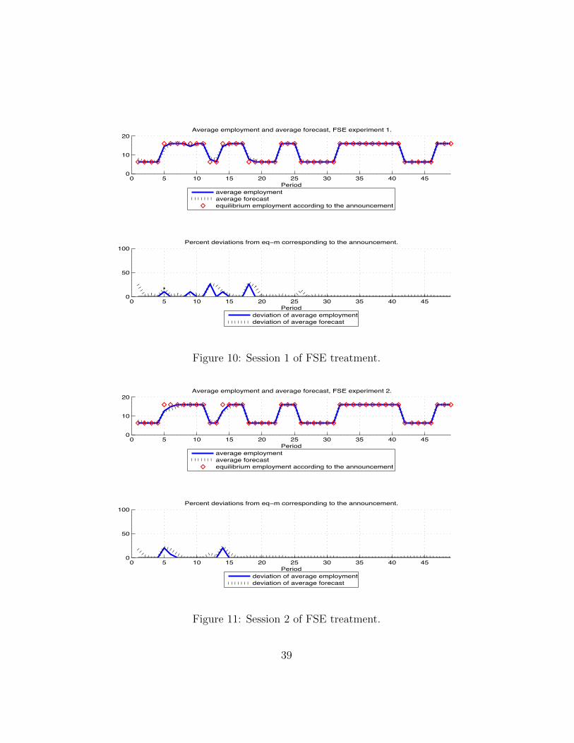
corresponding to the announcement.In sessions presented in Figures 10-12, 14, and 15, the experimental

economies exhibit close coordination on the announcements, and the per-centage deviations from the equilibrium corresponding to the announcementare zero during almost all periods. In these sessions, the subjects are re-warded for their forecasting accuracy only: as long as the subjects’ forecastsare close to the actual outcomes, they can get the maximum payoff, and itdoes not matter which steady state is the outcome as the steady states arenot payoff ranked. We can see better coordination on the announcementsand smaller deviations from the equilibrium employment than in the treat-ment with payoff based on profits. The formal test results are presented insection 5.3.

Figure 13 illustrates the results of session 6 in which we observe thatthe subjects coordinated on the low-employment steady state by the end ofthe session. During periods 14-17, 23-25, 32-41 and 47-49 the subjects ig-nored high-employment announcements and remained in the low-employmentsteady state. The lack of coordination on the high-employment announce-ment does not cost these subjects lower payoffs because they are rewarded fortheir forecasting accuracy only. Therefore, it is less of a puzzle in comparisonto the sessions in which the payoffs are based on profits.

In summary, in the sessions with payoff based on FSE we observe bothcoordination on the extrinsic announcements and coordination on the low-employment equilibrium. It is interesting to observe coordination on an-nouncements in this treatment because the subjects could have ignored theannouncements and stayed in one of the two equilibria, and they still wouldhave achieved the maximum payoff. It is a matter of coordination in thisgame, and the subjects coordinated on the announcements in many sessions.

5.3 Comparison of the two treatments

Next, we analyze the data and compare the two treatments. We want toevaluate how closely the experimental economies coordinate on the announce-ments and whether there is a difference between the two treatments.

5.3.1 Employment and forecasts

We pool the data on individual employment in periods with the low-employmentannouncements and in periods with the high-employment announcements

19

separately, and pool these data for all experimental sessions for each treat-ment. Table 1 presents the fractions of observations in the ranges containingtwo equilibria; this table corresponds to the histograms presented in Figures16 and 17.

The top left panel of Figure 16 represents the histogram of individual em-ployment decisions during periods with high-employment announcements inthe FSE treatment and shows that employment is concentrated on the high-employment equilibrium of 16 (83.54% of employment outcomes accordingto Table 1). The top right panel of Figure 16 presents the histogram of indi-vidual employment decisions during periods with low-employment announce-ments in the FSE treatment and illustrates that the values of employment areheavily concentrated on the low-employment equilibrium of 6.25 (98.23% ofoutcomes according to Table 1). The bottom left and right panels of Figure16 present the histograms of individual employment decisions during periodswith high-employment (bottom left) and low-employment announcements(bottom right) in the Profits treatment. These histograms also illustrate thatthe values of employment are very close to the equilibrium values correspond-ing to the announcements. During periods with high-employment announce-ments, 76.03% of the employment outcomes are close to the high-equilibriumemployment of 16; and during periods with low-employment announcements,88.76% of the employment outcomes are close to the low-equilibrium employ-ment of 6.25.

We also pool the data on the individual forecasts made in periods withlow-employment and in periods with high-employment announcements sep-arately. The top left and right panels of Figure 17 present the histogramsof individual forecasts made in periods with high- and low-employment an-nouncements in the FSE treatment and show that the forecasts are heav-ily concentrated on the respective equilibrium values corresponding to theannouncements: 61.83% of forecasts are in the range containing the high-equilibrium employment of 16, and 70.20% of forecasts correspond to thelow-equilibrium employment of 6.25. The bottom left and right panels ofFigure 17 present the histograms of individual forecasts made in periodswith high- and low-employment announcements in the Profits treatment andshow that the forecasts are centered around the equilibrium values, but thefractions of forecasts in the ranges containing equilibria are much lower thanin the FSE treatment: 28.60% of forecasts are in the range containing thehigh-equilibrium employment of 16, and 33.46% of the forecasts are in therange containing the low-equilibrium employment of 6.25. In the Profits

20

treatment, the subjects’ performance is not evaluated based on the accuracyof their forecasts, therefore, we observe very high variability in the forecasts.We will explore this in more detail in the next section 5.3.2.

Table 2 presents the data on average, median and standard deviations ofemployment and forecasts in both treatments.

5.3.2 Deviations from the equilibrium employment

We would like to test how closely subjects coordinate on the announcements.We compute the percentage deviations of employment and forecasts from theequilibrium corresponding to the announcement for all periods and pool thedata over all sessions for each treatment. Then we test whether the twotreatments are different.

The left panel of Figure 18 presents the cumulative density function(CDF) of the percentage deviations of individual forecasts from equilibriumemployment corresponding to the announcements in both treatments. TheCDF for the FSE treatment is larger than the CDF for the Profits treat-ment, which is statistically significant using the Kolmogorov-Smirnov test(with a p-value of 0, and test statistic of 0.3827). This implies that fore-casts are closer to the equilibrium values in the FSE treatment than in theProfits treatment. As the subjects are rewarded based on the accuracy oftheir forecasts in the FSE treatment, their forecasts are closer to the equi-librium values than those in the Profits treatment. As illustrated by Figure1, when forecasts are below 11.5, employment is constant at 6.25; and whenforecasts are above 13, employment is constant at 16. Thus, even if thesubjects’ forecasts are not equal to equilibrium employment, but are in theappropriate range, their employment outcomes and profits take equilibriumvalues corresponding to the low or high equilibrium. Thus the subjects in theProfits treatment do not have to make very accurate forecasts to arrive atequilibrium employment and profits. The shape of the employment functionexplains why forecasts are less accurate in the Profits treatment than in theFSE treatment.

The right panel of Figure 18 presents the CDF of the percentage devia-tions of individual employment outcomes from the equilibrium employmentcorresponding to the announcements in both treatments (Figure 1 explainswhy the lowest value of employment is 6.25 and the highest value is 16). TheCDF for the FSE treatment is larger than the CDF for the Profits treatment,which is statistically significant using Kolmogorov-Smirnov test (with p-value

21

of 0, and test statistic of 0.0839). This implies that employment outcomesare closer to the equilibrium values in the FSE treatment than in the Profitstreatment. Forecast decisions are closer to the equilibrium values in the FSEtreatment than in the Profits treatment. Because employment outcomes arebased on forecasts, employment is also closer to the equilibrium employmentin the FSE treatment than in the Profits treatment.

6 Further discussion of adaptive learning

The results of our experiments exhibit a large degree of consistency with theadaptive learning theory results described in Section 3.3, which is a theorythat motivated our experimental study. There it was shown that an SSEfluctuating between nH and nL is locally stable under learning, as are thesteady states nH and nL themselves. In our practice periods we ensured thatsubjects saw a strong correlation between the announcement At and reportedaverage employment of others, N̄t. In many of the experimental sessionsthis was sufficient to generate convergence or approximate convergence tothe SSE throughout the experimental session. In this section, we providedescriptive evidence about behavior of subjects suggestive of learning duringthe experiment.19

For example in the Profits treatment, sessions 1 to 3, we see initial de-viations from the SSE in early periods, with a process of learning in whichsubjects eventually closely approximate the SSE. This is seen also in session4 of Profits treatment, but with larger initial errors: the extended sequenceof nine high announcements between periods 32 and 41, followed by five lowannouncements between periods 42 and 46, appear to have been helpful ininducing apparent eventual convergence to the SSE.

Even the cases in which there were substantial deviations from the announcement-based SSE are illuminating in terms of adaptive learning. In session 5 of theProfits treatment, subjects appear less certain about the relevance of theannouncement. During the sequence of high announcements between peri-ods 14 –17 and 23 – 25, forecasts are significantly below nM = 12.5, whichimplies that actual observations of average employment are less than theaverage forecast, which under adaptive learning pushes agents towards nLrather than nH . However, during the extended sequence of high announce-

19This descriptive evidence can be useful as a motivation for a formal testing of learningmechanisms by subjects which is outside the scope of this study.

22

ments in periods 32-41, subjects relearn the high equilibrium and continueto make high forecasts during the subsequent low announcements. At theend of session 5 it appears possible that subjects have converged on the highsteady state. These results might be consistent with some of the subjectsconditioning their learning rule on the announcements, with other subjectsdisregarding the announcements and instead using a simple non-conditionaladaptive learning rule. In session 6 we see a similar pattern, except that inthe middle part of the high announcement periods 32-41, expectations areslightly lower and this means that the even lower observed N̄t pushes fore-casts down toward the low steady state. At the end of session 6 it appearspossible that subjects have converged on the low steady state.

Similar interpretation can be given to the FSE sessions. Evidence of adap-tive learning is seen in several of them, particularly of the forecast of averageemployment during periods of high announcements early in the experimentalsession. Where there is apparent convergence to the SSE, the convergence isquite close in several of the FSE sessions. In session 4 of the FSE treatment,however, there appears clearly to be eventual convergence to the low steadystate. This again might be consistent with a substantial proportion of thesubjects using non-conditional adaptive learning rules.

The adaptive learning framework described and discussed in Section 3.3can be extended in various ways. For example, one can allow for heteroge-nous priors of subjects, i.e. allow for different subjects to have differentinitial expectations and degrees of subjective uncertainty about their fore-casts. Furthermore, more general adaptive learning rules along the line ofEvans, Honkapohja and Marimon (2001), allow for heterogeneity in gains, in-ertia and experimentation. This can greatly increase the variety of possiblepaths under adaptive learning, and lead to more subtle learning dynamicsin which heterogeneous expectations can emerge. Our results appear to beconsistent with such generalized adaptive learning rules.

6.1 The role of heterogeneity in learning

Continuing with this last point, we note that when agents have heteroge-neous expectations, learning dynamics can depend on the dispersion of ex-pectations as well as on the average forecast. For example, even if, when theannouncement is high, most agents have expectations near the high steadystate, if there are several agents that have sufficiently low expectations, this

23

can be enough to destabilize coordination on an SSE.20 Furthermore, underthe Profits treatment, it is possible that subjects understand that their lossfunction is not symmetric around a given equilibrium, and they may takethis feature into account when making their forecasts.21

Thus, how quickly subjects learn to coordinate on each announcementmay also be influenced by the fact that switching to high employment fromlow employment more quickly than other subjects is costlier in terms oflower profits than switching to low employment while other subjects stillchoose high employment. How profitable choosing high or low employmentis depends on how many subjects choose high and low values.

With our parametrization, choosing high employment is relatively moreprofitable than choosing low employment when five out of six subjects choosehigh values (see Table 3). In contrast, if two or more subjects out of six chooselow employment, they get higher profit than those who choose high employ-ment. Thus, the coordination on the announcement about high employmentis more demanding in terms of how many subjects need to coordinate (five outof six) to make coordination on high employment profitable. And the coordi-nation on low employment is relatively simpler: it requires only two subjectsfollowing the announcement about low employment to make choosing lowemployment more profitable. The technical reason for this asymmetry is thefunctional form of the production function and the calibration of positiveproduction externality. The square root production function was chosen asa simple production function with diminishing returns, and form and cali-bration of production externality and wage rate were chosen to be as simpleas possible and calibrated to yield three well-spaced Pareto-ranked steadystates. Well-spaced steady states were needed for easy identification of thecorrespondence of experimental results with the equilibria and for easy un-derstanding by the subjects. Given these design constraints, the asymmetryof the basins of attraction was difficult to avoid. With heterogeneous fore-casts, the ”basin of attraction” is a complicated multidimensional object,and can be a subject for future research.

Let us take a closer look at how learning happens during an experimental

20More formally, the basin of attraction of an SSE, in terms of initial expectations,depends on the dispersion of these expectations as well as on the mean.

21“Direct criterion” versions of the adaptive learning rules, described in Section 3.3, canbe developed in which decisions or forecasts are adjusted in the direction of the decisionor forecast that would have been most profitable in the preceding period. For an example,see Woodford (1990).

24

session and at the role of heterogeneity. For example, in session 4 of theProfits treatment (Figure 7) during periods 23-26 with high announcements,the subjects fail to coordinate on high employment as only two or threesubjects choose high values. Next in periods 32-41, four, then five and even-tually all six subjects choose high values. During the final sequence of highannouncements in periods 47-50, all subjects choose high values after oneperiod of high announcements. Similarly, subjects learn in periods with lowannouncements. During periods 12-13, three and then four subjects chooselow values. In periods 18-21, three subjects choose low values in period 18,and then all the subjects choose low values. Next in periods 26-31, five sub-jects choose low values immediately, and then all subjects choose low values.Thus, we can see that as the session proceeds it takes fewer periods for sub-jects to coordinate on the announcements, i.e. the subjects learn during theexperiment.

However, coordination on the announcements does not always happen.In session 6 (Figure 13) subjects coordinate on the low value by the endof the session. During periods 32-41 with high announcements, only twoor three subjects choose high values. This makes choosing the low valuemore profitable, and eventually all subjects choose low values. When notenough subjects choose high values, lower profits drive them towards the lowequilibrium.

Similar dynamics are present in the FSE treatment. Coordination on thehigh-employment equilibrium is more demanding because it requires five outof six subjects to choose high values for the system dynamics to be driventowards the high equilibrium. When less than five subjects choose highvalues, average employment of others is below their forecasts which underadaptive learning pushes them towards low equilibrium.

In session 2 of the FSE treatment (Figure 11) during periods 5-11 and14-17 with high announcements, the subjects learn to forecast high valuesafter two periods during which four and then five subjects choose high val-ues. In periods 23-25, all subjects choose high values, and in period 25 allsubjects learn the exact high-equilibrium value. In periods 32-41, everybodychooses high-equilibrium value after one period of high announcements. Dur-ing the final sequence of high announcements, all subjects choose the high-equilibrium values. Similarly, the subjects learn to choose low-equilibriumvalues during periods with low announcements. During periods 12-13, allsubjects choose low forecasts which are quite heterogeneous. In periods 18-22, four and then five subjects choose the low-equilibrium value of 6.25 while

25

one chooses 7. This behavior continues during the remaining periods withlow announcements (26-31 and 42-46).

In session 4 of the FSE treatment (Figure 13) subjects ignore the an-nouncements and coordinate on the low equilibrium. It is interesting that atthe beginning of this session during periods 5-11 with high announcements,all subjects choose high values. However, their forecasts are heterogeneous(14.25, 14.35, 15, 17, 13.8, 15). In periods 14-17, only one subject tries thehigh value for two periods and then switches to the low value. Next in pe-riods 23-25, all the subjects choose low, heterogeneous forecasts resulting inlow employment, and in the subsequent periods with high announcements,the forecasts are equal to the low-equilibrium value or very close to it.

7 Conclusion

We have conducted experiments in a simple, stylized macroeconomic modelwith a production externality that generates multiple equilibria. The equilib-ria are payoff-ranked – the low-employment equilibrium has lower profit thanthe medium or high-employment equilibria do – which adds to the challengefor coordination and switching between them. We observe that subjects canindeed coordinate on extraneous announcements (a ‘sunspot’ equilibrium),with switching between low- and high-employment states, in treatments withtwo different payoff structures. When subjects payoffs are evaluated basedon forecast squared error (FSE treatment), their forecasts and employmentoutcomes are closer to the equilibrium corresponding to the announcementthan they are in the treatment based on the profits. This is explained by thefunctional form of the employment and a reward based on the accuracy ofthe forecasts.

In our set-up coordination on the sunspot equilibrium is Pareto rankedsuperior to coordination on the low equilibrium but inferior to coordinationon the high equilibrium. It is striking that in our set-up we appear ableto induce subjects to coordinate on sunspot equilibria in a high proportionof the sessions, and that this occurs even when there exists an equilibriumsteady state that would provide higher payoffs to all agents. However, thestability of the sunspot equilibria under adaptive learning is local, and wealso see experiments in which subjects appear to eventually coordinate on thelow or high steady state. Our results raise a number of important questions.What would happen if the initial experience obtained in training session were

26

different? Will the results be robust to the form of the externality? Howwould agents react if there were a regime change in which the number ofsteady states were reduced to one? Can our results be extended to dynamicversions of the model in which agents need to forecast both the level of currentemployment and the average level of employment next period? We reservethese questions and other extensions to future research.

References

[1] Adam, K. 2007. Experimental Evidence on the Persistence of Outputand Inflation. Economic Journal. 117, 603-636.

[2] Arifovic, J.1995. Genetic Algorithms and Inflationary Economies. Jour-nal of Monetary Economics. 36, 219-243.

[3] Arifovic, J. 1996. The Behavior of the Exchange Rate in the GeneticAlgorithm and Experimental Economies. Journal of Political Economy.104, 510-541.

[4] Arifovic, J., Duffy, J. 2018. Heterogeneous Agent Modeling: Experi-mental Evidence, in: Hommes, C., LeBaron, B. (Eds.), Handbook ofComputational Economics, Volume 4, Amsterdam: North-Holland, pp.491-540.

[5] Azariadis, C., Guesnerie, R. 1986. Sunspots and Cycles. Review of Eco-nomic Studies. 53, 725-737.

[6] Bao, T., C. Hommes, Duffy, J. 2013. Learning, Forecasting and Optimiz-ing: an Experimental Study. European Economic Review. 61, 186-204.

[7] Bao, Te, Hommes, C., Sonnemans, J., Tuinstra, J. 2012. Individual ex-pectations, limited rationality and aggregate outcomes. Journal of Eco-nomic Dynamics and Control. 36, 1101-1120.

[8] Benhabib, J. and R. Farmer. 1994.Indeterminacy and Increasing Re-turns. Journal of Economic Theory. 63, 19-41.

[9] Benhabib, J., Schmidt-Grohe, S., Uribe, M. 2001. The perils of Taylor-rules. Journal of Economic Theory. 96, 40-69.

27

[10] Beugnot, J., Gurguc, Z., Ovlisen, F. Roose, and M. Roos. 2012. Coor-dination Failure Caused by Sunspots. Economic Bulletin. 32 (4), 2860-2869.

[11] Capra, M., Tanaka, T., Camerer, C., Feiler, L., Sovero, V., Nous-sair, C.N. 2009. The Impact of Simple Institutions in ExperimentalEconomies with Poverty Traps. Economic Journal. 119(539), 977-1009

[12] Cass, D., Shell, K. 1983. Do Sunspots Matter? Journal of PoliticalEconomy. 91, 193-227.

[13] Clarida, R., Gali, J., Gertler, M. 2000. Monetary Policy Rules andMacroeconomic Stability: Evidence and Some Theory. Quarterly Jour-nal of Economics. 115, 147-180.

[14] Coibion, O., Gorodnichenko,Y., Kumar, S. 2018. “How do firms formtheir expectations? New survey evidence. American Economic Review.108, 2671-2713.

[15] Cooper, R., John, A. 1988. Coordinating Coordination Failures in Key-nesian Models. Quarterly Journal of Economics. 113, 441-464.

[16] Cooper, R., D. DeJong, Forsythe, R., T. Ross, T. 1990. Selection Cri-teria in Coordination Games: Some Experimental Results. AmericanEconomic Review. 80 (1), 218-233.

[17] Cooper, R. W., DeJong, D. V., Forsythe, R., Ross, T.W. 1992. Commu-nication in Coordination Games. Quarterly Journal of Economics. 107,739-771.

[18] Corbae, D., Duffy, J.. 2008. Experiments with Network Formation.Games and Economic Behavior. 64, 81-120.

[19] Duffy, J. 2016. Macroeconomics: A Survey of Laboratory Research,in: J.H. Kagel and A.E. Roth (Eds.), Handbook of Experimental Eco-nomics. Volume 2, Princeton University Press, Princeton, pp. 1-90.

[20] Duffy, J., Feltovich, N. 2010. Correlated Equilibria, Good and Bad: AnExperimental Study. International Economic Review. 51, 701-721.

[21] Duffy, J., Fisher, E. 2005. Sunspots in the Laboratory. American Eco-nomic Review. 95, 510-529.

28

[22] Ehrmann, M.,Pfajfar,D., Santoro, E. 2017. Consumer attitudes and theirinflation expectations. Journal of Central Banking. 13, 225-259.

[23] Evans, G., Honkapohja, S. 1995. Increasing Social Return, Learning andBifurcation Phenomena, in: Kirman, A., Salmon, M. (Eds.), Learningand Rationality in Economics, Blackwell, Oxford, pp. 216–235.

[24] Evans, G., Honkapohja, S. 1994. On the Local Stability of Sunspot Equi-libria under Adaptive Learning. Journal of Economic Theory. 64, 142-161.

[25] Evans, G., Honkapohja, S.. 2001. Learning and Expectations in Macro-conomics, Princeton: Princeton University Press.

[26] Evans, G., Honkapohja, S., Marimon, R. 2001. Convergence in MonetaryInflation Models with Hetergeneous Learning Rules. Macroeconomic Dy-namics. 5, 1-31.

[27] Evans, G., Honkapohja, S., Marimon, R. 2007. Stable Sunspot Equilibriain a Cash-in-Advance Economy. The B.E. Journal of Macroeconomics,Advances. 7 (1), Article 3.

[28] Evans, G., Honkapohja, S., Romer, P. 1998. Growth Cycles. AmericanEconomic Review 88, 495-515.

[29] Farmer, Roger. 1999. The Macroeconomics of Self-Fulfilling Prophecies,second ed. MIT Press, Cambridge.

[30] Farmer, 2015. Global sunspots and asset prices in a monetary economy.NBER working paper No 20831.

[31] Fehr, D., Heinemann, F., Llorente-Saguer, A. 2018. The Power ofSunspots: An Experimental Analysis. Journal of Monetary Economics.

[32] Fischbacher, U. 2007. Z-Tree: Zurich Toolbox for Ready-made EconomicExperiments. Experimental Economics. 10 (2), 171-178.

[33] Gali, J., 2014). Monetary policy and rational asset price bubbles. Amer-ican Economic Review. 104, 721-752.

29

[34] Garratt, R., Keister, T. 2009. Bank runs as coordination failures: anexperimental study. Journal of Economic Behavior and Organization.71, 300-317.

[35] Honkapohja, S., Mitra, K. 2004. Are non-fundamental equilibria learn-able in models of monetary policy. Journal of Monetary Economics. 51,1743-1770.

[36] Heinemann, F., Nagel, R., Ockenfels, P. 2004. The Theory of GlobalGames on Test: Experimental Analysis of Coordination Games withPublic and Private Information. Econometrica. 72, 1583–1599.

[37] Howitt, P., McAfee, R.P. 1992. Animal Spirits. American Economic Re-view. 82, 493-507.

[38] Lei, V., Noussair, C.N. 2002. An Experimental Test of an OptimalGrowth Model. American Economic Review. 92(3), 549-570.

[39] Lei, V., Noussair, C.N. 2007. Equilibrium Selection in an ExperimentalMacroeconomy. Southern Economic Journal. 74, 448-482.

[40] Lim, S.S., E. Prescott, E., S. Sunder, S. 1994. Stationary Solution to theOverlapping Generations Model of Fiat Money: Experimental Evidence.Empirical Economics. 19, 255-77.

[41] Marimon, R., Sunder, S. 1993. Indeterminacy of Equilibria in a Hyperin-flationary World: Experimental Evidence. Econometrica. 61, 1073-1107.

[42] Marimon, R., Sunder, S. 1994. Expectations and Learning under Al-ternative Monetary Regimes: An Experimental Approach. EconomicTheory. 4, 131-62.

[43] Marimon, R., Sunder, S. 1995. Does a Constant Money Growth RuleHelp Stabilize Inflation? Carnegie-Rochester Conference Series on Pub-lic Policy. 43, 111-156.

[44] Marimon, R., Spear, S.E., Sunder, S. 1993. Expectationally Driven Mar-ket Volatility: An Experimental Study. Journal of Economic Theory. 61,74-103.

30

[45] McGough, B., Q. Meng, Q., Xue, J. 2013. Expectational stability ofsunspot equilibria in non-convex economies. Journal of Economic Dy-namics and Control. 37, 1126-1141.

[46] Mertens, M., Ravn, M.O. 2014. Fiscal Policy in an Expectations-DrivenLiquidity Trap. Review of Economic Studies. 81, 1637–1667

[47] Miao, J., Shen, Z., Wang,P. 2019. Monetary Policy and Rational AssetBubbles: Comments. American Economic Review. 109(5), 1969-1990.

[48] Shea, P., 2013. Learning By Doing, Short-Sightedness, and Indetermi-nacy. Economic Journal. 123, 738-763.

[49] Schotter, A., Yorulmazer, T. 2009. On the Severity of Bank Runs: AnExperimental Study. Journal of Financial Intermediation. 18, 217-241.

[50] Van Huyck, J. B., Battalio, R. C., Beil, R.O. 1990. Tacit Coordina-tion Games, Strategic Uncertainty, and Coordination Failure. AmericanEconomic Review. 80(1), 234-48.

[51] Woodford, M. 1990. Learning to Believe in Sunspots. Econometrica. 58,277-307.

31

Table 1: Percentage of observations in each range of values.

range FSE treatment Profits treatmentE, H E, L F, H F, L E, H E, L F, H F, L

5.5-6.5 14.71 98.23 10.19 70.20 17.28 88.76 2.78 33.4615.5-16.5 83.54 1.64 61.83 1.14 76.03 8.84 28.60 1.77

Note: E, H = employment during periods with high-employment announcements;E, L = employment during low announcements; F, H = forecasts during highannouncements; F, L = forecasts during low announcements.

Table 2: Descriptive statistics of the data.

High-employment announcements Low-employment announcementsEmployment average median std skewness average median std skewness

FSE 14.46 16.00 3.51 -1.86 6.42 6.25 1.27 7.34Profits 13.91 16.00 3.83 -1.36 7.20 6.25 2.81 2.73

Forecasts average median std skewness average median std skewnessFSE 14.35 16.00 3.21 -1.84 6.66 6.25 1.37 4.78

Profits 14.21 15.00 3.30 -1.06 7.85 7.00 3.14 1.51

Table 3: Productivity and profits of subjects forecasting low and high values.

Number of forecasters Productivity of forecasters Profit of forecasterslow high low high low high6 0 2.5 - 3.125 -5 1 2.5 2.5 3.125 24 2 2.5 2.5 3.125 23 3 3.1 2.5 4.65 22 4 4.0 3.1 6.87 4.41 5 4.0 4.0 6.87 80 6 - 4.0 - 8

32

0 2 4 6 8 10 12 14 16 18 200

2

4

6

8

10

12

14

16

18

20

Forecast of average employment of others

Optim

al em

ploym

ent

Optimal employment as a function of forecast

Figure 1: This figures presents employment as a function of forecast of aver-age employment of others according to equation 1.

33

Figure 2: Screenshot for Profit treatment.

34

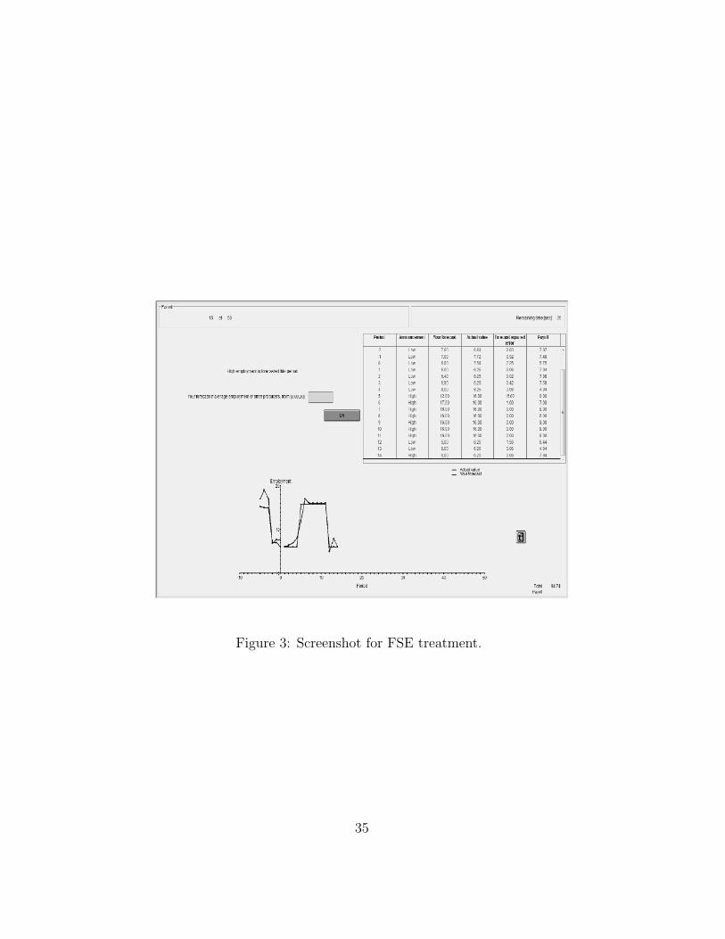
Figure 3: Screenshot for FSE treatment.

35

0 5 10 15 20 25 30 35 40 450

10

20

Period

Average employment and average forecast, Profits experiment 1, Nov 2011.

average employmentaverage forecastequilibrium employment according to the announcement

0 5 10 15 20 25 30 35 40 450

50

100

Period

Percent deviations from eq−m corresponding to the announcement.

deviation of average employmentdeviation of average forecast

Figure 4: Session 1 of profits treatment.

0 5 10 15 20 25 30 35 40 450

10

20

Period



0 5 10 15 20 25 30 35 40 450

50

100

Period



Figure 5: Session 2 of Profits treatment.

36

0 5 10 15 20 25 30 35 40 450

10

20

Period



0 5 10 15 20 25 30 35 40 450

50

100

Period




0 5 10 15 20 25 30 35 40 450

10

20

Period



0 5 10 15 20 25 30 35 40 450

50

100

Period




37

0 5 10 15 20 25 30 35 40 450

10

20

Period



0 5 10 15 20 25 30 35 40 450

50

100

Period




0 5 10 15 20 25 30 35 40 450

10

20

Period



0 5 10 15 20 25 30 35 40 450

50

100

Period




38

0 5 10 15 20 25 30 35 40 450

10

20

Period

Average employment and average forecast, FSE experiment 1.


0 5 10 15 20 25 30 35 40 450

50

100

Period



Figure 10: Session 1 of FSE treatment.

0 5 10 15 20 25 30 35 40 450

10

20

Period



0 5 10 15 20 25 30 35 40 450

50

100

Period




39

0 5 10 15 20 25 30 35 40 450

10

20

Period



0 5 10 15 20 25 30 35 40 450

50

100

Period




0 5 10 15 20 25 30 35 40 450

10

20

Period



0 5 10 15 20 25 30 35 40 450

50

100

Period




40

0 5 10 15 20 25 30 35 40 450

10

20

Period



0 5 10 15 20 25 30 35 40 450

50

100

Period




0 5 10 15 20 25 30 35 40 450

10

20

Period



0 5 10 15 20 25 30 35 40 450

50

100

Period




41

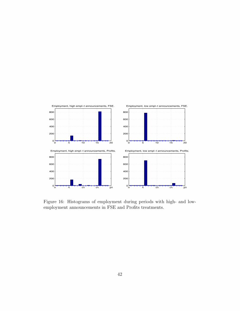
0 5 10 15 200

200

400

600

800

Employment, high empl−t announcements, FSE.

0 5 10 15 200

200

400

600

800

Employment, low empl−t announcements, FSE.

0 5 10 15 200

200

400

600

800

Employment, high empl−t announcements, Profits.

0 5 10 15 200

200

400

600

800

Employment, low empl−t announcements, Profits.

Figure 16: Histograms of employment during periods with high- and low-employment announcements in FSE and Profits treatments.

42

0 5 10 15 200

200

400

600

800

Forecasts, high empl−t announcements, FSE.

0 5 10 15 200

200

400

600

800

Forecasts, low empl−t announcements, FSE.

0 5 10 15 200

200

400

600

800

Forecasts, high empl−t announcements, Profits.

0 5 10 15 200

200

400

600

800

Forecasts, low empl−t announcements, Profits.

Figure 17: Histograms of forecasts during periods with high- and low-employment announcements in FSE and profits treatments.

0 20 40 60 80 1000

0.2

0.4

0.6

0.8

1

Percent deviations, x

F(x)

= pr

ob(d

evia

tions

≤ x

)

Deviations of forecasts

0 20 40 60 80 1000

0.2

0.4

0.6

0.8

1

Percent deviations, x

F(x)

= pr

ob(d

evia

tions

≤ x

)

Deviations of employment

FSE treatmentProfits treatment

0 20 40 60 80 100 1200

0.2

0.4

0.6

0.8

1

Values of efficiency, x

F(x)

= pr

ob(e

fficie

ncy ≤

x)

Efficiency based on FSE.

0 20 40 60 80 100 1200

0.2

0.4

0.6

0.8

1

Values of efficiency, x

F(x)

= pr

ob(e

fficie

ncy ≤

x)

Efficiency based on the profits.

Figure 18: Cumulative density functions of deviations of forecasts andemployment from equilibrium employment corresponding to the announce-ments.

43

are sunspots learnable? an experimental investigation in a

Documents