1

AREA UNDER A CURVE

The two big ideas in calculus are the tangent line problem and the area problem.  In the tangent line problem, you saw how the limit process could be applied to the slope of a line to find the slope of a general curve.  A second classic problem in calculus is in finding the area of a plane region that is bounded by the graphs of functions.  In this case, the limit process is applied to the area of a rectangle to find the area of a general region.

A basic overview of “areas as limits.”  In the “limit of rectangles” approach, we take the area under a curve y = f (x) above the interval [a , b] by approximating a collection of inscribed or circumscribed rectangles is such a way that the more rectangles used, the better the approximation.  Finally, the number of rectangles is increased without limit and, bingo, we get the area! Now known as integration.Specifically, we are interested in finding the area A of a region bounded by the x‐axis, the graph of a nonnegative function y = f (x) defined on some interval [a, b].

Note: The requirement that f be non‐negative on [a, b] means that no portion of its graph on the interval is below the x‐axis.  By using rectangles, we can see that there are three different ways of approximating the area for A.  This method is commonly known as Riemann Sums.

2

DEFINITION:

Let f be continuous on [a, b] and f(x) ≥ 0 for all x in the interval. We define the area A under the graph on the interval to be:

This is the summation definition of the area between the curve and the x­axis.  We use a less conceptual way of estimating the area.

3

General Solution Method for inscribed or circumscribed rectangles (Lower and Upper sums):

1. Draw a rough graph of the function over the interval.

2. Use formula                               to determine each                                                                         subinterval length.

3. Compute x­coordinates of rectangles at either left­end         or right­end.4. Compute the areas of each rectangle (inscribed or         circumscribed).5. Find summation of the approximated areas of the         rectangles.

4

EX #1:  Approximate the area under the curve of              above the interval [2, 5] by dividing [2, 5] into n = 4              subintervals of equal length and computing

Step 2:  Determine subinterval width

Step 3:  Compute points of subdivision

Step 4:  Since f is increasing the minimum value for f(x)               on each subinterval occurs at the left endpoint.

f (c1)=

Height of each rectangle:

f (c2)=

f (c3)= f (c4)=

Step 5:  Calculate area of each rectangle.

f (c1) Δx =

f (c4) Δx =

f (c2) Δx =

f (c3) Δx =

INSCRIBED RECTANGLES:  Because the graph is increasing, inscribed rectangles will be formed using the left endpoint of each rectangle to calculate the height.

a)  the sum of the areas of inscribed rectangles (lower sums)

b)  the sum of the areas of circumscribed rectangles (upper sums)

Step 1:  Sketch

Step 6: Summation of interval is the sum of the    areas of all four rectangles 

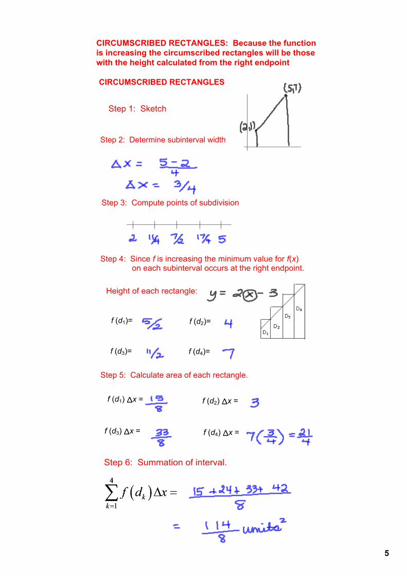
5

CIRCUMSCRIBED RECTANGLES

Step 2:  Determine subinterval width

Step 3:  Compute points of subdivision

Step 4:  Since f is increasing the minimum value for f(x)               on each subinterval occurs at the right endpoint.

f (d1)=

Height of each rectangle:

f (d2)=

f (d3)= f (d4)=

Step 5:  Calculate area of each rectangle.

f (d1) Δx =

f (d3) Δx = f (d4) Δx =

f (d2) Δx =

Step 6:  Summation of interval.

CIRCUMSCRIBED RECTANGLES:  Because the function is increasing the circumscribed rectangles will be those with the height calculated from the right endpoint

Step 1:  Sketch

6

EX #2:                     Approximate the area under the curve ofabove the interval [0, 2] by dividing the interval into n = 5 subintervals of equal length using inscribed and circumscribed rectangles.

7

EX #3:                     Approximate the area, A, under the graph ofon the interval [0, 4]. 

8

EX #4:                     Approximate the area, A, under the graph ofon the interval