argall dissertation
DESCRIPTION
RoboticsTRANSCRIPT

LEARNING MOBILE ROBOT MOTION CONTROLFROM DEMONSTRATION AND CORRECTIVE
FEEDBACK
Brenna D. Argall
CMU-RI-TR-09-13
Submitted in partial fulfilment ofthe requirements for the degree of
Doctor of Philosophy
Robotics InstituteCarnegie Mellon University
Pittsburgh, PA 15213
March 2009
Thesis Committee:Brett Browning, Co-ChairManuela Veloso, Co-Chair
J. Andrew BagnellChuck T. Thorpe
Maja J. Mataric, University of Southern California
c© Brenna D. Argall, MMIX

ii

ABSTRACT
Fundamental to the successful, autonomous operation of mobile robots are robust motion controlalgorithms. Motion control algorithms determine an appropriate action to take based on the
current state of the world. A robot observes the world through sensors, and executes physicalactions through actuation mechanisms. Sensors are noisy and can mislead, however, and actionsare non-deterministic and thus execute with uncertainty. Furthermore, the trajectories producedby the physical motion devices of mobile robots are complex, which make them difficult to modeland treat with traditional control approaches. Thus, to develop motion control algorithms formobile robots poses a significant challenge, even for simple motion behaviors. As behaviors becomemore complex, the generation of appropriate control algorithms only becomes more challenging. Todevelop sophisticated motion behaviors for a dynamically balancing differential drive mobile robotis one target application for this thesis work. Not only are the desired behaviors complex, butprior experiences developing motion behaviors through traditional means for this robot proved tobe tedious and demand a high level of expertise.
One approach that mitigates many of these challenges is to develop motion control algorithmswithin a Learning from Demonstration (LfD) paradigm. Here, a behavior is represented as pairsof states and actions; more specifically, the states encountered and actions executed by a teacherduring demonstration of the motion behavior. The control algorithm is generated from the robotlearning a policy, or mapping from world observations to robot actions, that is able to reproducethe demonstrated motion behavior. Robot executions with any policy, including those learned fromdemonstration, may at times exhibit poor performance; for example, when encountering areas ofthe state-space unseen during demonstration. Execution experience of this sort can be used by ateacher to correct and update a policy, and thus improve performance and robustness.
The approaches for motion control algorithm development introduced in this thesis pair demon-stration learning with human feedback on execution experience. The contributed feedback frameworkdoes not require revisiting areas of the execution space in order to provide feedback, a key advantagefor mobile robot behaviors, for which revisiting an exact state can be expensive and often impossible.The types of feedback this thesis introduces range from binary indications of performance qualityto execution corrections. In particular, advice-operators are a mechanism through which continu-ous-valued corrections are provided for multiple execution points. The advice-operator formulationis thus appropriate for low-level motion control, which operates in continuous-valued action spacessampled at high frequency.
This thesis contributes multiple algorithms that develop motion control policies for mobile robotbehaviors, and incorporate feedback in various ways. Our algorithms use feedback to refine demon-strated policies, as well as to build new policies through the scaffolding of simple motion behaviorslearned from demonstration. We evaluate our algorithms empirically, both within simulated motioncontrol domains and on a real robot. We show that feedback improves policy performance on simplebehaviors, and enables policy execution of more complex behaviors. Results with the Segway RMProbot confirm the effectiveness of the algorithms in developing and correcting motion control policieson a mobile robot.


FUNDING SOURCES
We gratefully acknowledge the sponsors of this research, without whom this thesis would not havebeen possible:
• The Boeing Corporation, under Grant No. CMU-BA-GTA-1.
• The Qatar Foundation for Education, Science and Community Development.
• The Department of the Interior, under Grant No. NBCH1040007.
The views and conclusions contained in this document are those of the author and should notbe interpreted as representing the official policies, either expressed or implied, of any sponsoringinstitution, the U.S. government or any other entity.

ACKNOWLEDGEMENTS
There are many to thank in connection with this dissertation, and to begin I must acknowledge myadvisors. Throughout the years they have critically assessed my research while supporting both meany my work, extracting strengths and weaknesses alike, and have taught me to do the same. InBrett I have been fortunate to have an advisor who provided an extraordinary level of attentionto, and hands on guidance in, the building of my knowledge and skill base, who ever encouragedme to think bigger and strive for greater achievements. I am grateful to Manuela for her insightsand big-picture guidance, for the excitement she continues to show for and build around my thesisresearch, and most importantly for reminding me what we are and are not in the business of doing.Thank you also to my committee members, Drew Bagnell, Chuck Thorpe and Maja Mataric for thetime and thought they put into the direction and assessment of this thesis.
The Carnegie Mellon robotics community as a whole has been a wonderful and supportivegroup. I am grateful to all past and present co-collaborators on the various Segway RMP projects(Jeremy, Yang, Kristina, Matt, Hatem), and Treasure Hunt team members (Gil, Mark, Balajee,Freddie, Thomas, Matt), for companionship in countless hours of robot testing and in the frustrationof broken networks and broken robots. I acknowledge Gil especially, for invariably providing hisbalanced perspective, and thank Sonia for all of the quick questions and reference checks. Thankyou to all of the Robotics Institute and School of Computer Science staff, who do such a great jobsupporting us students.
I owe a huge debt to all of my teachers throughout the years, who shared with me theirknowledge and skills, supported inquisitive and critical thought, and underlined that the ability tolearn is more useful than facts; thank you for making me a better thinker. I am especially gratefulto my childhood piano teachers, whose approach to instruction that combines demonstration anditerative corrections provided much inspiration for this thesis work.
To the compound and all of its visitors, for contributing so instrumentally to the richness ofmy life beyond campus, I am forever thankful. Especially to Lauren, for being the best backyardneighbor, and to Pete, for being a great partner with which to explore the neighborhood and world,not to mention for providing invaluable support through the highs and lows of this dissertationdevelopment. To the city of Pittsburgh, home of many wonderful organizations in which I have beenfortunate to take part, and host to many forgotten, fascinating spots which I have been delightedto discover. Graduate school was much more fun that it was supposed to be.
Last, but very certainly not least, I am grateful to my family, for their love and supportthroughout all phases of my life that have led to this point. I thank my siblings - Alyssa, Evan, Lacey,Claire, Jonathan and Brigitte - for enduring my childhood bossiness, for their continuing friendship,and for pairing nearly every situation with laughter, however snarky. I thank my parents, Amy andDan, for so actively encouraging my learning and education: from answering annoyingly exhaustivechildhood questions and sending me to great schools, through to showing interest in foreign topicslike robotics research. I am lucky to have you all, and this dissertation could not have happenedwithout you.


DEDICATION
To my grandparents
Frances, Big Jim, Dell and Clancy; for building the family of which I am so fortunate to be a part,and in memory of those who saw me begin this degree but will not see its completion.


TABLE OF CONTENTS
ABSTRACT . . . . . . . . . . . . . . . . . . . . . . . . . . . . . . . . . . . . . . . . . . . . . iii
FUNDING SOURCES . . . . . . . . . . . . . . . . . . . . . . . . . . . . . . . . . . . . . . . . v
ACKNOWLEDGEMENTS . . . . . . . . . . . . . . . . . . . . . . . . . . . . . . . . . . . . . vii
DEDICATION . . . . . . . . . . . . . . . . . . . . . . . . . . . . . . . . . . . . . . . . . . . . ix
LIST OF FIGURES . . . . . . . . . . . . . . . . . . . . . . . . . . . . . . . . . . . . . . . . . xv
LIST OF TABLES . . . . . . . . . . . . . . . . . . . . . . . . . . . . . . . . . . . . . . . . . . xvii
NOTATION . . . . . . . . . . . . . . . . . . . . . . . . . . . . . . . . . . . . . . . . . . . . . xix
CHAPTER 1. Introduction . . . . . . . . . . . . . . . . . . . . . . . . . . . . . . . . . . . . 11.1. Practical Approaches to Robot Motion Control . . . . . . . . . . . . . . . . . . . . . 1
1.1.1. Policy Development and Low-Level Motion Control . . . . . . . . . . . . . . . . 21.1.2. Learning from Demonstration . . . . . . . . . . . . . . . . . . . . . . . . . . . . 31.1.3. Control Policy Refinement . . . . . . . . . . . . . . . . . . . . . . . . . . . . . . 4
1.2. Approach . . . . . . . . . . . . . . . . . . . . . . . . . . . . . . . . . . . . . . . . . . 61.2.1. Algorithms Overview . . . . . . . . . . . . . . . . . . . . . . . . . . . . . . . . . 61.2.2. Results Overview . . . . . . . . . . . . . . . . . . . . . . . . . . . . . . . . . . . 7
1.3. Thesis Contributions . . . . . . . . . . . . . . . . . . . . . . . . . . . . . . . . . . . . 81.4. Document Outline . . . . . . . . . . . . . . . . . . . . . . . . . . . . . . . . . . . . . 9
CHAPTER 2. Policy Development and Execution Feedback . . . . . . . . . . . . . . . . . . 112.1. Policy Development . . . . . . . . . . . . . . . . . . . . . . . . . . . . . . . . . . . . 12
2.1.1. Learning from Demonstration . . . . . . . . . . . . . . . . . . . . . . . . . . . . 122.1.2. Dataset Limitations and Corrective Feedback . . . . . . . . . . . . . . . . . . . . 15
2.2. Design Decisions for a Feedback Framework . . . . . . . . . . . . . . . . . . . . . . . 152.2.1. Feedback Type . . . . . . . . . . . . . . . . . . . . . . . . . . . . . . . . . . . . . 162.2.2. Feedback Interface . . . . . . . . . . . . . . . . . . . . . . . . . . . . . . . . . . . 172.2.3. Feedback Incorporation . . . . . . . . . . . . . . . . . . . . . . . . . . . . . . . . 18
2.3. Our Feedback Framework . . . . . . . . . . . . . . . . . . . . . . . . . . . . . . . . . 192.3.1. Feedback Types . . . . . . . . . . . . . . . . . . . . . . . . . . . . . . . . . . . . 192.3.2. Feedback Interface . . . . . . . . . . . . . . . . . . . . . . . . . . . . . . . . . . . 202.3.3. Feedback Incorporation . . . . . . . . . . . . . . . . . . . . . . . . . . . . . . . . 222.3.4. Future Directions . . . . . . . . . . . . . . . . . . . . . . . . . . . . . . . . . . . 24
2.4. Our Baseline Feedback Algorithm . . . . . . . . . . . . . . . . . . . . . . . . . . . . . 242.4.1. Algorithm Overview . . . . . . . . . . . . . . . . . . . . . . . . . . . . . . . . . . 242.4.2. Algorithm Execution . . . . . . . . . . . . . . . . . . . . . . . . . . . . . . . . . 252.4.3. Requirements and Optimization . . . . . . . . . . . . . . . . . . . . . . . . . . . 27

TABLE OF CONTENTS
2.5. Summary . . . . . . . . . . . . . . . . . . . . . . . . . . . . . . . . . . . . . . . . . . 28
CHAPTER 3. Policy Improvement with Binary Feedback . . . . . . . . . . . . . . . . . . . 293.1. Algorithm: Binary Critiquing . . . . . . . . . . . . . . . . . . . . . . . . . . . . . . . 29
3.1.1. Crediting Behavior with Binary Feedback . . . . . . . . . . . . . . . . . . . . . . 293.1.2. Algorithm Execution . . . . . . . . . . . . . . . . . . . . . . . . . . . . . . . . . 31
3.2. Empirical Implementation . . . . . . . . . . . . . . . . . . . . . . . . . . . . . . . . . 323.2.1. Experimental Setup . . . . . . . . . . . . . . . . . . . . . . . . . . . . . . . . . . 323.2.2. Results . . . . . . . . . . . . . . . . . . . . . . . . . . . . . . . . . . . . . . . . . 34
3.3. Discussion . . . . . . . . . . . . . . . . . . . . . . . . . . . . . . . . . . . . . . . . . . 373.3.1. Conclusions . . . . . . . . . . . . . . . . . . . . . . . . . . . . . . . . . . . . . . 373.3.2. Future Directions . . . . . . . . . . . . . . . . . . . . . . . . . . . . . . . . . . . 37
3.4. Summary . . . . . . . . . . . . . . . . . . . . . . . . . . . . . . . . . . . . . . . . . . 38
CHAPTER 4. Advice-Operators . . . . . . . . . . . . . . . . . . . . . . . . . . . . . . . . . 414.1. Overview . . . . . . . . . . . . . . . . . . . . . . . . . . . . . . . . . . . . . . . . . . 42
4.1.1. Definition . . . . . . . . . . . . . . . . . . . . . . . . . . . . . . . . . . . . . . . . 424.1.2. Requirements for Development . . . . . . . . . . . . . . . . . . . . . . . . . . . . 42
4.2. A Principled Approach to Advice-Operator Development . . . . . . . . . . . . . . . . 434.2.1. Baseline Advice-Operators . . . . . . . . . . . . . . . . . . . . . . . . . . . . . . 434.2.2. Scaffolding Advice-Operators . . . . . . . . . . . . . . . . . . . . . . . . . . . . . 444.2.3. The Formulation of Synthesized Data . . . . . . . . . . . . . . . . . . . . . . . . 46
4.3. Comparison to More Mapping Examples . . . . . . . . . . . . . . . . . . . . . . . . . 484.3.1. Population of the Dataset . . . . . . . . . . . . . . . . . . . . . . . . . . . . . . . 484.3.2. Dataset Quality . . . . . . . . . . . . . . . . . . . . . . . . . . . . . . . . . . . . 51
4.4. Future Directions . . . . . . . . . . . . . . . . . . . . . . . . . . . . . . . . . . . . . . 524.4.1. Application to More Complex Spaces . . . . . . . . . . . . . . . . . . . . . . . . 524.4.2. Observation-modifying Operators . . . . . . . . . . . . . . . . . . . . . . . . . . 534.4.3. Feedback that Corrects Dataset Points . . . . . . . . . . . . . . . . . . . . . . . 54
4.5. Summary . . . . . . . . . . . . . . . . . . . . . . . . . . . . . . . . . . . . . . . . . . 54
CHAPTER 5. Policy Improvement with Corrective Feedback . . . . . . . . . . . . . . . . . 575.1. Algorithm: Advice-Operator Policy Improvement . . . . . . . . . . . . . . . . . . . . 58
5.1.1. Correcting Behavior with Advice-Operators . . . . . . . . . . . . . . . . . . . . . 585.1.2. Algorithm Execution . . . . . . . . . . . . . . . . . . . . . . . . . . . . . . . . . 59
5.2. Case Study Implementation . . . . . . . . . . . . . . . . . . . . . . . . . . . . . . . . 605.2.1. Experimental Setup . . . . . . . . . . . . . . . . . . . . . . . . . . . . . . . . . . 615.2.2. Results . . . . . . . . . . . . . . . . . . . . . . . . . . . . . . . . . . . . . . . . . 625.2.3. Discussion . . . . . . . . . . . . . . . . . . . . . . . . . . . . . . . . . . . . . . . 64
5.3. Empirical Robot Implementation . . . . . . . . . . . . . . . . . . . . . . . . . . . . . 665.3.1. Experimental Setup . . . . . . . . . . . . . . . . . . . . . . . . . . . . . . . . . . 665.3.2. Results . . . . . . . . . . . . . . . . . . . . . . . . . . . . . . . . . . . . . . . . . 68
5.4. Discussion . . . . . . . . . . . . . . . . . . . . . . . . . . . . . . . . . . . . . . . . . . 705.4.1. Conclusions . . . . . . . . . . . . . . . . . . . . . . . . . . . . . . . . . . . . . . 705.4.2. Future Directions . . . . . . . . . . . . . . . . . . . . . . . . . . . . . . . . . . . 72
5.5. Summary . . . . . . . . . . . . . . . . . . . . . . . . . . . . . . . . . . . . . . . . . . 73
CHAPTER 6. Policy Scaffolding with Feedback . . . . . . . . . . . . . . . . . . . . . . . . . 756.1. Algorithm: Feedback for Policy Scaffolding . . . . . . . . . . . . . . . . . . . . . . . 76
6.1.1. Building Behavior with Teacher Feedback . . . . . . . . . . . . . . . . . . . . . . 766.1.2. Feedback for Policy Scaffolding Algorithm Execution . . . . . . . . . . . . . . . 766.1.3. Scaffolding Multiple Policies . . . . . . . . . . . . . . . . . . . . . . . . . . . . . 80
xii

TABLE OF CONTENTS
6.2. Empirical Simulation Implementation . . . . . . . . . . . . . . . . . . . . . . . . . . 816.2.1. Experimental Setup . . . . . . . . . . . . . . . . . . . . . . . . . . . . . . . . . . 816.2.2. Results . . . . . . . . . . . . . . . . . . . . . . . . . . . . . . . . . . . . . . . . . 85
6.3. Discussion . . . . . . . . . . . . . . . . . . . . . . . . . . . . . . . . . . . . . . . . . . 926.3.1. Conclusions . . . . . . . . . . . . . . . . . . . . . . . . . . . . . . . . . . . . . . 926.3.2. Future Directions . . . . . . . . . . . . . . . . . . . . . . . . . . . . . . . . . . . 94
6.4. Summary . . . . . . . . . . . . . . . . . . . . . . . . . . . . . . . . . . . . . . . . . . 97
CHAPTER 7. Weighting Data and Feedback Sources . . . . . . . . . . . . . . . . . . . . . . 997.1. Algorithm: Demonstration Weight Learning . . . . . . . . . . . . . . . . . . . . . . . 100
7.1.1. Algorithm Execution . . . . . . . . . . . . . . . . . . . . . . . . . . . . . . . . . 1007.1.2. Weighting Multiple Data Sources . . . . . . . . . . . . . . . . . . . . . . . . . . 102
7.2. Empirical Simulation Implementation . . . . . . . . . . . . . . . . . . . . . . . . . . 1047.2.1. Experimental Setup . . . . . . . . . . . . . . . . . . . . . . . . . . . . . . . . . . 1047.2.2. Results . . . . . . . . . . . . . . . . . . . . . . . . . . . . . . . . . . . . . . . . . 106
7.3. Discussion . . . . . . . . . . . . . . . . . . . . . . . . . . . . . . . . . . . . . . . . . . 1087.3.1. Conclusions . . . . . . . . . . . . . . . . . . . . . . . . . . . . . . . . . . . . . . 1097.3.2. Future Directions . . . . . . . . . . . . . . . . . . . . . . . . . . . . . . . . . . . 110
7.4. Summary . . . . . . . . . . . . . . . . . . . . . . . . . . . . . . . . . . . . . . . . . . 110
CHAPTER 8. Robot Learning from Demonstration . . . . . . . . . . . . . . . . . . . . . . . 1138.1. Gathering Examples . . . . . . . . . . . . . . . . . . . . . . . . . . . . . . . . . . . . 114
8.1.1. Design Decisions . . . . . . . . . . . . . . . . . . . . . . . . . . . . . . . . . . . . 1148.1.2. Correspondence . . . . . . . . . . . . . . . . . . . . . . . . . . . . . . . . . . . . 1158.1.3. Demonstration . . . . . . . . . . . . . . . . . . . . . . . . . . . . . . . . . . . . . 1178.1.4. Imitation . . . . . . . . . . . . . . . . . . . . . . . . . . . . . . . . . . . . . . . . 1188.1.5. Other Approaches . . . . . . . . . . . . . . . . . . . . . . . . . . . . . . . . . . . 120
8.2. Deriving a Policy . . . . . . . . . . . . . . . . . . . . . . . . . . . . . . . . . . . . . . 1208.2.1. Design Decisions . . . . . . . . . . . . . . . . . . . . . . . . . . . . . . . . . . . . 1218.2.2. Problem Space Continuity . . . . . . . . . . . . . . . . . . . . . . . . . . . . . . 1228.2.3. Mapping Function . . . . . . . . . . . . . . . . . . . . . . . . . . . . . . . . . . . 1228.2.4. System Models . . . . . . . . . . . . . . . . . . . . . . . . . . . . . . . . . . . . . 1248.2.5. Plans . . . . . . . . . . . . . . . . . . . . . . . . . . . . . . . . . . . . . . . . . . 126
8.3. Summary . . . . . . . . . . . . . . . . . . . . . . . . . . . . . . . . . . . . . . . . . . 127
CHAPTER 9. Related Work . . . . . . . . . . . . . . . . . . . . . . . . . . . . . . . . . . . . 1299.1. LfD Topics Central to this Thesis . . . . . . . . . . . . . . . . . . . . . . . . . . . . . 129
9.1.1. Motion Control . . . . . . . . . . . . . . . . . . . . . . . . . . . . . . . . . . . . 1299.1.2. Behavior Primitives . . . . . . . . . . . . . . . . . . . . . . . . . . . . . . . . . . 1309.1.3. Multiple Demonstration Sources and Reliability . . . . . . . . . . . . . . . . . . 131
9.2. Limitations of the Demonstration Dataset . . . . . . . . . . . . . . . . . . . . . . . . 1319.2.1. Undemonstrated State . . . . . . . . . . . . . . . . . . . . . . . . . . . . . . . . 1319.2.2. Poor Quality Data . . . . . . . . . . . . . . . . . . . . . . . . . . . . . . . . . . . 132
9.3. Addressing Dataset Limitations . . . . . . . . . . . . . . . . . . . . . . . . . . . . . . 1339.3.1. More Demonstrations . . . . . . . . . . . . . . . . . . . . . . . . . . . . . . . . . 1349.3.2. Rewarding Executions . . . . . . . . . . . . . . . . . . . . . . . . . . . . . . . . . 1349.3.3. Correcting Executions . . . . . . . . . . . . . . . . . . . . . . . . . . . . . . . . . 1359.3.4. Other Approaches . . . . . . . . . . . . . . . . . . . . . . . . . . . . . . . . . . . 135
9.4. Summary . . . . . . . . . . . . . . . . . . . . . . . . . . . . . . . . . . . . . . . . . . 136
CHAPTER 10. Conclusions . . . . . . . . . . . . . . . . . . . . . . . . . . . . . . . . . . . . 13910.1. Feedback Techniques . . . . . . . . . . . . . . . . . . . . . . . . . . . . . . . . . . . 140
xiii

TABLE OF CONTENTS
10.1.1. Focused Feedback for Mobile Robot Policies . . . . . . . . . . . . . . . . . . . . 14010.1.2. Advice-Operators . . . . . . . . . . . . . . . . . . . . . . . . . . . . . . . . . . . 140
10.2. Algorithms and Empirical Results . . . . . . . . . . . . . . . . . . . . . . . . . . . . 14110.2.1. Binary Critiquing . . . . . . . . . . . . . . . . . . . . . . . . . . . . . . . . . . 14110.2.2. Advice-Operator Policy Improvement . . . . . . . . . . . . . . . . . . . . . . . 14110.2.3. Feedback for Policy Scaffolding . . . . . . . . . . . . . . . . . . . . . . . . . . . 14210.2.4. Demonstration Weight Learning . . . . . . . . . . . . . . . . . . . . . . . . . . 143
10.3. Contributions . . . . . . . . . . . . . . . . . . . . . . . . . . . . . . . . . . . . . . . 143
BIBLIOGRAPHY . . . . . . . . . . . . . . . . . . . . . . . . . . . . . . . . . . . . . . . . . . 145
xiv

LIST OF FIGURES
1.1 The Segway RMP robot. . . . . . . . . . . . . . . . . . . . . . . . . . . . . . . . . . . . . 3
2.1 Learning from Demonstration control policy derivation and execution. . . . . . . . . . . . 13
2.2 Example distribution of 1-NN distances within a demonstration dataset (black bars), andthe Poisson model approximation (red curve). . . . . . . . . . . . . . . . . . . . . . . . . 21
2.3 Example plot of the 2-D ground path of a learner execution, with color indications of datasetsupport (see text for details). . . . . . . . . . . . . . . . . . . . . . . . . . . . . . . . . . . 21
2.4 Policy derivation and execution under the general teacher feedback algorithm. . . . . . . 25
3.1 Policy derivation and execution under the Binary Critiquing algorithm. . . . . . . . . . . 30
3.2 Simulated robot motion (left) and ball interception task (right). . . . . . . . . . . . . . . 33
3.3 World state observations for the motion interception task. . . . . . . . . . . . . . . . . . 34
3.4 Example practice run, where execution efficiency improves with critiquing. . . . . . . . . 35
3.5 Improvement in successful interceptions, test set. . . . . . . . . . . . . . . . . . . . . . . . 36
4.1 Example applicability range of contributing advice-operators. . . . . . . . . . . . . . . . . 45
4.2 Advice-operator building interface, illustrated through an example (building the operatorAdjust Turn). . . . . . . . . . . . . . . . . . . . . . . . . . . . . . . . . . . . . . . . . . . 46
4.3 Distribution of observation-space distances between newly added datapoints and the nearestpoint within the existing dataset (histogram). . . . . . . . . . . . . . . . . . . . . . . . . 49
4.4 Plot of dataset points within the action space. . . . . . . . . . . . . . . . . . . . . . . . . 50
4.5 Number of points within each dataset across practice runs (see text for details). . . . . . 51
4.6 Performance improvement of the more-demonstration and feedback policies across practiceruns. . . . . . . . . . . . . . . . . . . . . . . . . . . . . . . . . . . . . . . . . . . . . . . . 52
5.1 Generating demonstration data under classical LfD (top) and A-OPI (bottom). . . . . . 58
5.2 Policy derivation and execution under the Advice-Operator Policy Improvement algorithm. 59
5.3 Segway RMP robot performing the spatial trajectory following task (approximate groundpath drawn in yellow). . . . . . . . . . . . . . . . . . . . . . . . . . . . . . . . . . . . . . 61
5.4 Execution trace mean position error compared to target sinusoidal trace. . . . . . . . . . 63
5.5 Example execution position traces for the spatial trajectory following task. . . . . . . . . 64
5.6 Using simple subgoal policies to gather demonstration data for the more complex sinusoid-following task. . . . . . . . . . . . . . . . . . . . . . . . . . . . . . . . . . . . . . . . . . . 65
5.7 Average test set error on target position (left) and heading (right), with the final policies. 69

LIST OF FIGURES
5.8 Average test set error on target position (left) and heading (right), with intermediatepolicies. . . . . . . . . . . . . . . . . . . . . . . . . . . . . . . . . . . . . . . . . . . . . . . 69
5.9 Dataset size growth with demonstration number. . . . . . . . . . . . . . . . . . . . . . . . 70
6.1 Policy derivation and execution under the Feedback for Policy Scaffolding algorithm. . . 796.2 Primitive subset regions (left) of the full racetrack (right). . . . . . . . . . . . . . . . . . 846.3 Percent task completion with each of the primitive behavior policies. . . . . . . . . . . . 866.4 Average translational execution speed with each of the primitive behavior policies. . . . . 866.5 Percent task completion during complex policy practice. . . . . . . . . . . . . . . . . . . . 876.6 Percent task completion with full track behavior policies. . . . . . . . . . . . . . . . . . . 886.7 Average and maximum translational (top) and rotational (bottom) speeds with full track
behavior policies. . . . . . . . . . . . . . . . . . . . . . . . . . . . . . . . . . . . . . . . . 906.8 Example complex driving task executions (rows), showing primitive behavior selection
(columns), see text for details. . . . . . . . . . . . . . . . . . . . . . . . . . . . . . . . . . 91
7.1 Policy derivation and execution under the Demonstration Weight Learning algorithm. . . 1007.2 Mean percent task completion and translational speed with exclusively one data source
(solid bars) and all sources with different weighting schemes (hashed bars). . . . . . . . . 1077.3 Data source learned weights (solid lines) and fractional population of the dataset (dashed
lines) during the learning practice runs. . . . . . . . . . . . . . . . . . . . . . . . . . . . . 1087.4 Percent task completion and mean translational speed during the practice runs. . . . . . 108
8.1 Categorization of approaches to building the demonstration dataset. . . . . . . . . . . . . 1148.2 Mapping a teacher execution to the learner. . . . . . . . . . . . . . . . . . . . . . . . . . 1158.3 Intersection of the record and embodiment mappings. . . . . . . . . . . . . . . . . . . . . 1168.4 Typical LfD approaches to policy derivation. . . . . . . . . . . . . . . . . . . . . . . . . . 1218.5 Categorization of approaches to learning a policy from demonstration data. . . . . . . . . 121
xvi
LIST OF TABLES
3.1 Pre- and post-feedback interception percent success, practice set. . . . . . . . . . . . . . . 363.2 Interception task success and efficiency, test set. . . . . . . . . . . . . . . . . . . . . . . . 36
5.1 Advice-operators for the spatial trajectory following task. . . . . . . . . . . . . . . . . . . 625.2 Average execution time (in seconds). . . . . . . . . . . . . . . . . . . . . . . . . . . . . . 635.3 Advice-operators for the spatial positioning task. . . . . . . . . . . . . . . . . . . . . . . . 675.4 Execution percent success, test set. . . . . . . . . . . . . . . . . . . . . . . . . . . . . . . 68
6.1 Advice-operators for the racetrack driving task. . . . . . . . . . . . . . . . . . . . . . . . 826.2 Execution performance of the primitive policies. . . . . . . . . . . . . . . . . . . . . . . . 856.3 Execution performance of the scaffolded policies. . . . . . . . . . . . . . . . . . . . . . . . 89
7.1 Advice-operators for the simplified racetrack driving task. . . . . . . . . . . . . . . . . . . 1057.2 Policies developed for the empirical evaluation of DWL. . . . . . . . . . . . . . . . . . . . 106


NOTATION
S : the set of world states, consisting of individual states s ∈ S
Z : the set of observations of world state, consisting of individual observations z ∈ Z
A : the set of robot actions, consisting of individual actions a ∈ A
T (s′|s, a) : a probabilistic mapping between states by way of actions
D : a set of teacher demonstrations, consisting of individual demonstrations d ∈ D
Π : a set of policies, consisting of individual policies π ∈ Π
Φ : indication of an execution trace segment
dΦ : the subset of datapoints within segment Φ of execution d, s.t. dΦ ⊆ d
z : general teacher feedback
c : specific teacher feedback of the performance credit type
op : specific teacher feedback of the advice-operator type
φ (, ) : a kernel distance function for regression computations
Σ−1 : a diagonal parameter matrix for regression computations
m : a scaling factor associated with each point in D under algorithm BC
ξ : label for a demonstration set, s.t. policy πξ derives from dataset Dξ; used to annotatebehavior primitives under algorithm FPS and data sources under algorithm DWL
Ξ : a set of demonstration set labels, consisting of individual labels ξ ∈ Ξ
τ : an indication of dataset support for a policy prediction under algorithm FPS
w : the set of data source weights under algorithm DWL, consisting of individual weightswξ ∈ w
r : reward (execution or state)
λ : parameter of the Poisson distribution modeling 1-NN distances between dataset points

NOTATION
µ : mean of a statistical distribution
σ : standard deviation of a statistical distribution
α, β, δ, ε, κ : implementation-specific parameters
(x, y, θ) : robot position and heading
(ν, ω) : robot translational and rotational speeds, respectively
gR (z, a) : LfD record mapping
gE (z, a) : LfD embodiment mapping
xx
CHAPTER 1
Introduction
Robust motion control algorithms are fundamental to the successful, autonomous operation ofmobile robots. Robot movement is enacted through a spectrum of mechanisms, from wheel
speeds to joint actuation. Even the simplest of movements can produce complex motion trajectories,and consequently robot motion control is known to be a difficult problem. Existing approaches thatdevelop motion control algorithms range from model-based control to machine learning techniques,and all require a high level of expertise and effort to implement. One approach that addresses manyof these challenges is to teach motion control through demonstration.
In this thesis, we contribute approaches for the development of motion control algorithms formobile robots, that build on the demonstration learning framework with the incorporation of humanfeedback. The types of feedback considered range from binary indications of performance quality toexecution corrections. In particular, one key contribution is a mechanism through which continuous-valued corrections are provided for motion control tasks. The use of feedback spans from refininglow-level motion control to building algorithms from simple motion behaviors. In our contributedalgorithms, teacher feedback augments demonstration to improve control algorithm performanceand enable new motion behaviors, and does so more effectively than demonstration alone.
1.1. Practical Approaches to Robot Motion Control
Whether an exploration rover in space or recreational robot for the home, successful autonomousmobile robot operation requires a motion control algorithm. A policy is one such control algorithmform, that maps observations of the world to actions available on the robot. This mapping isfundamental to many robotics applications, yet in general is complex to develop.
The development of control policies requires a significant measure of effort and expertise. Toimplement existing techniques for policy development frequently requires extensive prior knowledgeand parameter tuning. The required prior knowledge ranges from details of the robot and itsmovement mechanisms, to details of the execution domain and how to implement a given controlalgorithm. Any successful application typically has the algorithm highly tuned for operation with aparticular robot in a specific domain. Furthermore, existing approaches are often applicable only tosimple tasks due to computation or task representation constraints.

CHAPTER 1. INTRODUCTION
1.1.1. Policy Development and Low-Level Motion Control
The state-action mapping represented by a motion policy is typically complex to develop. Onereason for this complexity is that the target observation-action mapping is unknown. What is knownis the desired robot motion behavior, and this behavior must somehow be represented throughan unknown observation-action mapping. How accurately the policy derivation techniques thenreproduce the mapping is a separate and additional challenge. A second reason for this complexityare the complications of motion policy execution in real world environments. In particular:
1. The world is observed through sensors, which are typically noisy and thus may provideinconsistent or misleading information.
2. Models of world dynamics are an approximation to the true dynamics, and are oftenfurther simplified due to computational or memory constraints. These models thus mayinaccurately predict motion effects.
3. Actions are motions executed with real hardware, which depends on many physical con-siderations such as calibration accuracy and necessarily executes actions with some levelof imprecision.
All of these considerations contribute to the inherent uncertainty of policy execution in the realworld. The net result is a difference between the expected and actual policy execution.
Traditional approaches to robot control model the domain dynamics and derive policies usingthese mathematical models. Though theoretically well-founded, these approaches depend heavilyupon the accuracy of the model. Not only does this model require considerable expertise to develop,but approximations such as linearization are often introduced for computational tractability, therebydegrading performance. Other approaches, such as Reinforcement Learning, guide policy learning byproviding reward feedback about the desirability of visiting particular states. To define a functionto provide these rewards, however, is known to be a difficult problem that also requires considerableexpertise to address. Furthermore, building the policy requires gathering information by visitingstates to receive rewards, which is non-trivial for a mobile robot learner executing actual actions inthe real world.
Motion control policy mappings are able to represent actions at a variety of control levels.
Low-level actions: Low-level actions directly control the movement mechanisms of the ro-bot. These actions are in general continuous-valued and of short time duration, and alow-level motion policy is sampled at a high frequency.
High-level actions: High-level actions encode a more abstract action representation, whichis then translated through other means to affect the movement mechanisms of the robot;for example, through another controller. These actions are in general discrete-valued and oflonger time duration, and their associated control policies are sampled at a low frequency.
2

1.1 PRACTICAL APPROACHES TO ROBOT MOTION CONTROL
In this thesis, we focus on low-level motion control policies. The continuous action-space and highsampling rate of low-level control are all key considerations during policy development.
The particular robot platform used to validate the approaches of this thesis is a Segway RobotMobility Platform (Segway RMP), pictured in Figure 1.1. The Segway RMP is a two-wheeleddynamically-balancing differential drive robot (Nguyen et al., 2004). The robot balancing mechanismis founded on inverse pendulum dynamics, the details of which are proprietary information of theSegway LLC company and are essentially unknown to us. The absence of details fundamental tothe robot motion mechanism, like the balancing controller, complicates the development of motionbehaviors for this robot, and in particular the application of dynamics-model-based motion controltechniques. Furthermore, this robot operates in complex environments that demand sophisticatedmotion behaviors. Our developed behavior architecture for this robot functions as a finite statemachine, where high-level behaviors are built on a hierarchy of other behaviors. In our previouswork, each low-level motion behavior was developed and extensively tuned by hand.
Figure 1.1. The Segway RMP robot.
The experience of personally developing numerous motion behaviors by hand for this robot (Ar-gall et al., 2006, 2007b), and subsequent desire for more straightforward policy development tech-niques, was a strong motivating factor in this thesis. Similar frustrations have been observed inother roboticists, further underlining the value of approaches that ease the policy development pro-cess. Another, more hypothetical, motivating factor is that as familiarity with robots within generalsociety becomes more prevalent, it is expected that future robot operators will include those who arenot robotics experts. We anticipate a future requirement for policy development approaches thatnot only ease the development process for experts, but are accessible to non-experts as well. Thisthesis represents a step towards this goal.
1.1.2. Learning from Demonstration
Learning from Demonstration (LfD) is a policy development technique with the potential forboth application to non-trivial tasks and straightforward use by robotics-experts and non-experts
3

CHAPTER 1. INTRODUCTION
alike. Under the LfD paradigm, a teacher first demonstrates a desired behavior to the robot, pro-ducing an example state-action trace. The robot then generalizes from these examples to learn astate-action mapping and thus derive a policy.
LfD has many attractive points for both learner and teacher. LfD formulations typically do notrequire expert knowledge of the domain dynamics, which removes performance brittleness resultingfrom model simplifications. The relaxation of the expert knowledge requirement also opens policydevelopment to non-robotics-experts, satisfying a need which we expect will increase as robotsbecome more common within general society. Furthermore, demonstration has the attractive featureof being an intuitive medium for communication from humans, who already use demonstration toteach other humans.
More concretely, the application LfD to motion control has a variety of advantages:
Implicit behavior to mapping translation: By demonstrating a desired motion behav-ior, and recording the encountered states and actions, the translation of a behavior into arepresentative state-action mapping is immediate and implicit. This translation thereforedoes not need to be explicitly identified and defined by the policy developer.
Robustness under real world uncertainty: The uncertainty of the real world meansthat multiple demonstrations of the same behavior will not execute identically. Gener-alization over examples therefore produces a policy that does not depend on a strictlydeterministic world, and thus will execute more robustly under real world uncertainty.
Focused policies: Demonstration has the practical feature of focusing the dataset of ex-amples to areas of the state-action space actually encountered during behavior execution.This is particularly useful in continuous-valued action domains, with an infinite numberof state-action combinations.
LfD has enabled successful policy development for a variety of robot platforms and applications.This approach is not without its limitations, however. Common sources of LfD limitations include:
1. Suboptimal or ambiguous teacher demonstrations.
2. Uncovered areas of the state space, absent from the demonstration dataset.
3. Poor translation from teacher to learner, due to differences in sensing or actuation.
This last source relates to the broad issue of correspondence between the teacher and learner, whomay differ in sensing or motion capabilities. In this thesis, we focus on demonstration techniquesthat do not exhibit strong correspondence issues.
1.1.3. Control Policy Refinement
A robot will likely encounter many states during execution, and to develop a policy that ap-propriately responds to all world conditions is difficult. Such a policy would require that the policydeveloper had prior knowledge of which world states would be visited, an unlikely scenario within
4

1.1 PRACTICAL APPROACHES TO ROBOT MOTION CONTROL
real-world domains, in addition to knowing the correct action to take from each of these states.An approach that circumvents this requirement is to refine a policy in response to robot executionexperience. Policy refinement from execution experience requires both a mechanism for evaluatingan execution, as well as a framework through which execution experience may be used to updatethe policy.
Executing a policy provides information about the task, domain and the effects of policy ex-ecution of this task in the given domain. Unless a policy is already optimal for every state in theworld, this execution information can be used to refine and improve the policy. Policy refinementfrom execution experience requires both detecting the relevant information, for example observing afailure state, and also incorporating the information into a policy update, for example producing apolicy that avoids the failure state. Learning from Experience, where execution experience is used toupdate the learner policy, allows for increased policy robustness and improved policy performance.A variety of mechanisms may be employed to learn from experience, including the incorporation ofperformance feedback, policy corrections or new examples of good behavior.
One approach to learning from experience has an external source offer performance feedbackon a policy execution. For example, feedback could indicate specific areas of poor or good policyperformance, which is one feedback approach considered in this thesis. Another feedback formulationcould draw attention to elements of the environment that are important for task execution.
Within the broad topic of machine learning, performance feedback provided to a learner typi-cally takes the form of state reward, as in Reinforcement Learning. State rewards provide the learnerwith an indication of the desirability of visiting a particular state. To determine whether a differentstate would have been more desirable to visit instead, alternate states must be visited, which canbe unfocused and intractable to optimize when working on real robot systems in motion controldomains with an infinite number of world state-action combinations. State rewards are generallyprovided automatically by the system and tend to be sparse, for example zero for all states exceptthose near the goal. One challenge to operating in worlds with sparse reward functions is the issueof reward back-propagation; that is, of crediting key early states in the execution for leading to aparticular reward state.
An alternative to overall performance feedback is to provide a correction on the policy execution,which is another feedback form considered in this thesis. Given a current state, such informationcould indicate a preferred action to take, or a preferred state into which to transition, for example.Determining which correction to provide is typically a task sufficiently complex to preclude a simplesparse function from providing a correction, and thus prompting the need for a human in the feedbackloop. The complexity of a correction formulation grows with the size of the state-action space, andbecomes particularly challenging in continuous state-action domains.
Another policy refinement technique, particular to LfD, provides the learner with more teacherdemonstrations, or more examples of good behavior executions. The goal of this approach is toprovide examples that clarify ambiguous teacher demonstrations or visit previously undemonstratedareas of the state-space. Having the teacher provide more examples, however, is unable to addressall sources of LfD error, for example correspondence issues or suboptimal teacher performance.The more-demonstrations approach also requires revisiting the target state in order to provide a
5

CHAPTER 1. INTRODUCTION
demonstration, which can be non-trivial for large state-spaces such as motion control domains. Thetarget state may be difficult, dangerous or even impossible to access. Furthermore, the motion pathtaken to visit the state can constitute a poor example of the desired policy behavior.
1.2. Approach
This thesis contributes an effective LfD framework to address common limitations of LfD thatcannot improve through further demonstration alone. Our techniques build and refine motion con-trol policies using a combination of demonstration and human feedback, which takes a variety offorms. Of particular note is the contributed formulation of advice-operators, which correct policyexecutions within continuous-valued, motion control domains. Our feedback techniques build andrefine individual policies, as well as facilitate the incorporation of multiple policies into the executionof more complex tasks. The thesis validates the introduced policy development techniques in bothsimulated and real robot domains.
1.2.1. Algorithms Overview
This work introduces algorithms that build policies through a combination of demonstrationand teacher feedback. The document first presents algorithms that are novel in the type of feedbackprovided; these are the Binary Critiquing and Advice-Operator Policy Improvement algorithms.This presentation is followed with algorithms that are novel in their incorporation of feedback intoa complex behavior policy; these are the Feedback for Policy Scaffolding and Demonstration WeightLearning algorithms.
In the first algorithm, Binary Critiquing (BC), the human teacher flags poorly performing areasof learner executions. The learner uses this information to modify its policy, by penalizing the under-lying demonstration data that supported the flagged areas. The penalization technique addressesthe issue of suboptimal or ambiguous teacher demonstrations. This sort of feedback is arguablywell-suited for human teachers, as humans are generally good at assigning basic performance creditto executions.
In the second algorithm, Advice-Operator Policy Improvement (A-OPI), a richer feedback isprovided by having the human teacher provide corrections on the learner executions. This is incontrast to BC, where poor performance is only flagged and the correct action to take is not indicated.In A-OPI the learner uses corrections to synthesize new data based on its own executions, andincorporates this data into its policy. Data synthesis can address the LfD limitation of datasetsparsity, and the A-OPI synthesis technique provides an alternate source for data - a key novelfeature of the A-OPI algorithm - that does not derive from teacher demonstrations. Providing analternative to teacher demonstration addresses the LfD limitation of teacher-learner correspondence,as well as suboptimal teacher demonstrations. To provide corrective feedback the teacher selectsfrom a finite predefined list of corrections, named advice-operators. This feedback is translated by thelearner into continuous-valued corrections suitable for modifying low-level motion control actions,which is the target application domain for this work.
The third algorithm, Feedback for Policy Scaffolding (FPS), incorporates feedback into a policybuilt from simple behavior policies. Both the built-up policy and the simple policies incorporate
6
1.2 APPROACH
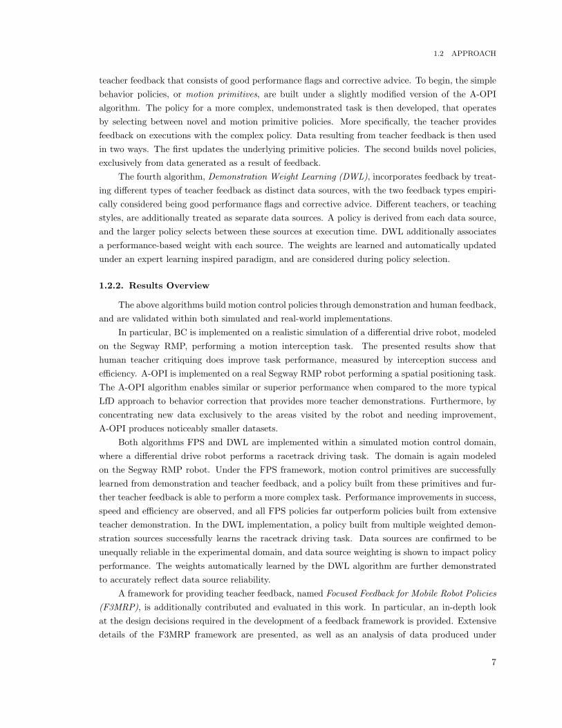
teacher feedback that consists of good performance flags and corrective advice. To begin, the simplebehavior policies, or motion primitives, are built under a slightly modified version of the A-OPIalgorithm. The policy for a more complex, undemonstrated task is then developed, that operatesby selecting between novel and motion primitive policies. More specifically, the teacher providesfeedback on executions with the complex policy. Data resulting from teacher feedback is then usedin two ways. The first updates the underlying primitive policies. The second builds novel policies,exclusively from data generated as a result of feedback.
The fourth algorithm, Demonstration Weight Learning (DWL), incorporates feedback by treat-ing different types of teacher feedback as distinct data sources, with the two feedback types empiri-cally considered being good performance flags and corrective advice. Different teachers, or teachingstyles, are additionally treated as separate data sources. A policy is derived from each data source,and the larger policy selects between these sources at execution time. DWL additionally associatesa performance-based weight with each source. The weights are learned and automatically updatedunder an expert learning inspired paradigm, and are considered during policy selection.
1.2.2. Results Overview
The above algorithms build motion control policies through demonstration and human feedback,and are validated within both simulated and real-world implementations.
In particular, BC is implemented on a realistic simulation of a differential drive robot, modeledon the Segway RMP, performing a motion interception task. The presented results show thathuman teacher critiquing does improve task performance, measured by interception success andefficiency. A-OPI is implemented on a real Segway RMP robot performing a spatial positioning task.The A-OPI algorithm enables similar or superior performance when compared to the more typicalLfD approach to behavior correction that provides more teacher demonstrations. Furthermore, byconcentrating new data exclusively to the areas visited by the robot and needing improvement,A-OPI produces noticeably smaller datasets.
Both algorithms FPS and DWL are implemented within a simulated motion control domain,where a differential drive robot performs a racetrack driving task. The domain is again modeledon the Segway RMP robot. Under the FPS framework, motion control primitives are successfullylearned from demonstration and teacher feedback, and a policy built from these primitives and fur-ther teacher feedback is able to perform a more complex task. Performance improvements in success,speed and efficiency are observed, and all FPS policies far outperform policies built from extensiveteacher demonstration. In the DWL implementation, a policy built from multiple weighted demon-stration sources successfully learns the racetrack driving task. Data sources are confirmed to beunequally reliable in the experimental domain, and data source weighting is shown to impact policyperformance. The weights automatically learned by the DWL algorithm are further demonstratedto accurately reflect data source reliability.
A framework for providing teacher feedback, named Focused Feedback for Mobile Robot Policies(F3MRP), is additionally contributed and evaluated in this work. In particular, an in-depth lookat the design decisions required in the development of a feedback framework is provided. Extensivedetails of the F3MRP framework are presented, as well as an analysis of data produced under
7

CHAPTER 1. INTRODUCTION
this framework and in particular resulting from corrective advice. Within the presentation of thiscorrective feedback technique, named advice-operators, a principled approach to their developmentis additionally contributed.
1.3. Thesis Contributions
This thesis considers the following research questions:
How might teacher feedback be used to address and correct common Learningfrom Demonstration limitations in low-level motion control policies?
In what ways might the resulting feedback techniques be incorporated into morecomplex policy behaviors?
To address common limitations of LfD, this thesis contributes mechanisms for providing humanfeedback, in the form of performance flags and corrective advice, and algorithms that incorporatethese feedback techniques. For the incorporation into more complex policy behaviors, human feed-back is used in the following ways: to build and correct demonstrated policy primitives; to link theexecution of policy primitives and correct these linkages; and to produce policies that are consideredalong with demonstrated policies during the complex motion behavior execution.
The contributions of this thesis are the following.
Advice-Operators: A feedback formulation that enables the correction of continuous-valuedpolicies. An in-depth analysis of correcting policies with in continuous action spaces, andthe data produced by our technique, is also provided.
Framework Focused Feedback for Mobile Robot Policies: A policy improvement frame-work for the incorporation of teacher feedback on learner executions, that allows for theapplication of a single piece of feedback over multiple execution points.
Algorithm Binary Critiquing : An algorithm that uses teacher feedback in the form ofbinary performance flags to refine motion control policies within a demonstration learningframework.
Algorithm Advice-Operator Policy Improvement : An algorithm that uses teacher feed-back in the form of corrective advice to refine motion control policies within a demonstra-tion learning framework.
Algorithm Feedback for Policy Scaffolding : An algorithm that uses multiple forms ofteacher feedback to scaffold primitive behavior policies, learned through demonstration,into a policy that exhibits a more complex behavior.
Algorithm Demonstration Weight Learning : An algorithm that considers multiple formsof teacher feedback as individual data sources, along with multiple demonstrators, andlearns to select between sources based on reliability.
8

1.4 DOCUMENT OUTLINE
Empirical Validation: The algorithms of this thesis are all empirically implemented andevaluated, within both real world - using a Segway RMP robot - and simulated motioncontrol domains.
Learning from Demonstration Categorization: A framework for the categorization oftechniques typically used in robot Learning from Demonstration.
1.4. Document Outline
The work of this thesis is organized into the following chapters.
Chapter 2: Overviews the LfD formulation of this thesis, identifies the design decisionsinvolved in building a feedback framework, and details the contributed Focused Feedbackfor Mobile Robot Policies framework along with our baseline feedback algorithm.
Chapter 3: Introduces the Binary Critiquing algorithm, and presents empirical results alongwith a discussion of binary putative feedback.
Chapter 4: Presents the contributed advice-operator technique along with an empiricalcomparison to an exclusively demonstration technique, and introduces an approach forthe principled development of advice-operators.
Chapter 5: Introduces the Advice-Operator Policy Improvement algorithm, presents theresults from an empirical case study as well as a full task implementation, and provides adiscussion of corrective feedback in continuous-action domains.
Chapter 6: Introduces the Feedback for Policy Scaffolding algorithm, presents an empiricalvalidation from building both motion primitive and complex policy behaviors, and providesa discussion of the use of teacher feedback to build complex motion behaviors.
Chapter 7: Introduces the Demonstration Weight Learning algorithm, and presents em-pirical results along with a discussion of the performance differences between multipledemonstration sources.
Chapter 8: Presents our contributed LfD categorization framework, along with a placementof relevant literature within this categorization.
Chapter 9: Presents published literature relevant to the topics addressed, and techniquesdeveloped, in this thesis.
Chapter 10: Overviews the conclusions of this work.
9


CHAPTER 2
Policy Development and Execution Feedback
Policy development is typically a complex process that requires a large investment in expertiseand time on the part of the policy designer. Even with a carefully crafted policy, a robot often
will not behave as the designer expects or intends in all areas of the execution space. One wayto address behavior shortcomings is to update a policy based on execution experience, which canincrease policy robustness and overall performance. For example, such an update may expand thestate-space in which the policy operates, or increase the likelihood of successful task completion.Many policy updates depend on evaluations of execution performance. Human teacher feedback isone approach for providing a policy with performance evaluations.
This chapter identifies many of the design decisions involved in the development of a feedbackframework. We contribute the framework Focused Feedback for Mobile Robot Policies (F3MRP)as a mechanism through which a human teacher provides feedback on mobile robot motion controlexecutions. Through the F3MRP framework, teacher feedback updates the motion control policy of amobile robot. The F3MRP framework is distinguished by operating at the stage of low-level motioncontrol, where actions are continuous-valued and sampled at high frequency. Some noteworthycharacteristics of the F3MRP framework are the following. A visual presentation of the 2-D groundpath taken by the mobile robot serves as an interface through which the teacher selects segmentsof the execution to receive feedback, which simplifies the challenge of providing feedback to policiessampled at a high frequency. Visual indications of data support for the policy predictions assist theteacher in the selection of execution segments and feedback type. An interactive tagging mechanismenables close association between teacher feedback and the learner execution.
Our feedback techniques build on a Learning from Demonstration (LfD) framework. UnderLfD, examples of behavior execution by a teacher are provided to a student. In our work, thestudent derives a policy, or state-action mapping, from the dataset of these examples. This mappingenables the learner to select an action to execute based on the current world state, and thus providesa control algorithm for the target behavior. Though LfD has been successfully employed for a varietyof robotics applications (see Ch. 8), the approach is not without its limitations. This thesis aims toaddress limitations common to LfD, and in particular those that do not improve with more teacherdemonstration. Our approach for addressing LfD limitations is to provide human teacher feedbackon learner policy executions.

CHAPTER 2. POLICY DEVELOPMENT AND EXECUTION FEEDBACK
The following section provides a brief overview of policy development under LfD, including adelineation of the specific form LfD takes in this thesis. Section 2.2 identifies key design decisionsthat define a feedback framework. Our feedback framework, F3MRP, is then described in Section 2.3.We present our general feedback algorithm in Section 2.4, which provides a base for all algorithmspresented later in the document.
2.1. Policy Development
Successful autonomous robot operation requires a control algorithm to select actions based onthe current state of the world. Traditional approaches to robot control model world dynamics,and derive a mathematically-based policy (Stefani et al., 2001). Though theoretically well-founded,these approaches depend heavily upon the accuracy of the dynamics model. Not only does themodel require considerable expertise to develop, but approximations such as linearization are oftenintroduced for computational tractability, thereby degrading performance. In other approaches therobot learns a control algorithm, through the use of machine learning techniques. One such approachlearns control from executions of the target behavior demonstrated by a teacher.
2.1.1. Learning from Demonstration
Learning from Demonstration (LfD) is a technique for control algorithm development thatlearns a behavior from examples, or demonstrations, provided by a teacher. For our purposes, theseexamples are sequences of state-action pairs recorded during the teacher’s demonstration of a desiredrobot behavior. Algorithms then utilize this dataset of examples to derive a policy, or mapping fromworld states to robot actions, that reproduces the demonstrated behavior. The learned policyconstitutes a control algorithm for the behavior, and the robot uses this policy to select an actionbased on the observed world state.
Demonstration has the attractive feature of being an intuitive medium for human communica-tion, as well as focusing the dataset to areas of the state-space actually encountered during behaviorexecution. Since it does not require expert knowledge of the system dynamics, demonstration alsoopens policy development to non-robotics-experts. Here we present a brief overview of LfD and itsimplementation within this thesis; a more thorough review of LfD is provided in Chapter 8.
2.1.1.1. Problem Statement. Formally, we define the world to consist of states S andactions A, with the mapping between states by way of actions being defined by the probabilistictransition function T (s′|s, a) : S ×A× S → [0, 1]. We assume state to not be fully observable. Thelearner instead has access to observed state Z, through a mapping S → Z. A teacher demonstrationdj ∈ D is represented as nj pairs of observations and actions such that dj = {(zij ,aij)} ∈ D, zij ∈Z,aij ∈ A, i = 0 · · ·nj . Within the typical LfD paradigm, the set D of these demonstrations is thenprovided to the learner. No distinction is made within D between the individual teacher executionshowever, and so for succinctness we adopt the notation (zk,ak) ≡
(zij ,a
ij
). A policy π : Z → A, that
selects actions based on an observation of the current world state, or query point, is then derivedfrom the dataset D.
12

2.1 POLICY DEVELOPMENT
Figure 2.1 shows a schematic of teacher demonstration executions, followed policy derivationfrom the resultant dataset D and subsequent learner policy executions. Dashed lines indicate repet-itive flow, and therefore execution cycles performed multiple times.
Figure 2.1. Learning from Demonstration control policy derivation and execution.
The LfD approach to obtaining a policy is in contrast to other techniques in which a policy islearned from experience, for example building a policy based on data acquired through exploration,as in Reinforcement Learning (RL) (Sutton and Barto, 1998). Also note that a policy derived underLfD is necessarily defined only in those states encountered, and for those actions taken, during theexample executions.
2.1.1.2. Learning from Demonstration in this Thesis. The algorithms we contributein this thesis learn policies within a LfD framework. There are many design decisions involved inthe development of a LfD system, ranging from who executes a demonstration to how a policy isderived from the dataset examples. We discuss LfD design decisions in depth within Chapter 8. Herehowever we summarize the primary decisions made for the algorithms and empirical implementationsof this thesis:
• A teleoperation demonstration approach is taken, as this minimizes correspondence issuesand is reasonable on our robot platform.1
1Teleoperation is not necessarily reasonable for all robot platforms, for example those with high degrees of control
freedom; it is reasonable, however, for the wheeled motion of our robot platform, the Segway RMP.
13
CHAPTER 2. POLICY DEVELOPMENT AND EXECUTION FEEDBACK
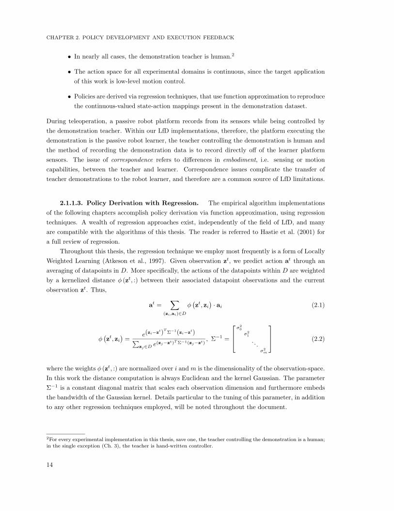
• In nearly all cases, the demonstration teacher is human.2
• The action space for all experimental domains is continuous, since the target applicationof this work is low-level motion control.
• Policies are derived via regression techniques, that use function approximation to reproducethe continuous-valued state-action mappings present in the demonstration dataset.
During teleoperation, a passive robot platform records from its sensors while being controlled bythe demonstration teacher. Within our LfD implementations, therefore, the platform executing thedemonstration is the passive robot learner, the teacher controlling the demonstration is human andthe method of recording the demonstration data is to record directly off of the learner platformsensors. The issue of correspondence refers to differences in embodiment, i.e. sensing or motioncapabilities, between the teacher and learner. Correspondence issues complicate the transfer ofteacher demonstrations to the robot learner, and therefore are a common source of LfD limitations.
2.1.1.3. Policy Derivation with Regression. The empirical algorithm implementationsof the following chapters accomplish policy derivation via function approximation, using regressiontechniques. A wealth of regression approaches exist, independently of the field of LfD, and manyare compatible with the algorithms of this thesis. The reader is referred to Hastie et al. (2001) fora full review of regression.
Throughout this thesis, the regression technique we employ most frequently is a form of LocallyWeighted Learning (Atkeson et al., 1997). Given observation zt, we predict action at through anaveraging of datapoints in D. More specifically, the actions of the datapoints within D are weightedby a kernelized distance φ (zt, :) between their associated datapoint observations and the currentobservation zt. Thus,
at =∑
(zi,ai)∈D
φ(zt, zi
)· ai (2.1)
φ(zt, zi
)=
e(zi−zt)TΣ−1(zi−zt)∑zj∈D e
(zj−zt)TΣ−1(zj−zt), Σ−1 =
σ20
σ21
. . .σ2m
(2.2)
where the weights φ (zt, :) are normalized over i and m is the dimensionality of the observation-space.In this work the distance computation is always Euclidean and the kernel Gaussian. The parameterΣ−1 is a constant diagonal matrix that scales each observation dimension and furthermore embedsthe bandwidth of the Gaussian kernel. Details particular to the tuning of this parameter, in additionto any other regression techniques employed, will be noted throughout the document.
2For every experimental implementation in this thesis, save one, the teacher controlling the demonstration is a human;
in the single exception (Ch. 3), the teacher is hand-written controller.
14
2.2 DESIGN DECISIONS FOR A FEEDBACK FRAMEWORK
2.1.2. Dataset Limitations and Corrective Feedback
LfD systems are inherently linked to the information provided in the demonstration dataset.As a result, learner performance is heavily limited by the quality of this information. One commoncause for poor learner performance is dataset sparsity, or the existence of areas of the state space inwhich no demonstration has been provided. A second cause is poor quality of the dataset examples,which can result from a teacher’s inability to perform the task optimally or from poor correspondencebetween the teacher and learner.
A primary focus of this thesis is to develop policy refinement techniques that address commonLfD dataset limitations, while being suitable for mobile robot motion control domains. The mobilityof the robot expands the state space, making more prevalent the issue of dataset sparsity. Low-level motion control implies domains with continuous-valued actions, sampled at a high frequency.Furthermore, we are particularly interested in refinement techniques that provide corrections withinthese domains.
Our contributed LfD policy correction techniques do not rely on teacher demonstration toexhibit the corrected behavior. Some strengths of this approach include the following:
No need to recreate state: This is especially useful if the world states where demonstra-tion is needed are dangerous (e.g. lead to a collision), or difficult to access (e.g. in themiddle of a motion trajectory).
Not limited by the demonstrator: Corrections are not limited to the execution abilitiesof the demonstration teacher, who may be suboptimal.
Unconstrained by correspondence: Corrections are not constrained by physical differ-ences between the teacher and learner.
Possible when demonstration is not: Further demonstration may actually be impossi-ble (e.g. rover teleoperation over a 40 minute Earth-Mars communications lag).
Other novel feedback forms also are contributed in this thesis, in addition to policy corrections.These feedback forms also do not require state revisitation.
We formulate corrective feedback as a predefined list of corrections, termed advice-operators.Advice-operators enable the translation of a statically-defined high-level correction into a continuous-valued, execution-dependent, low-level correction; Chapter 4 will present advice-operators in detail.Furthermore, when combined with our techniques for providing feedback (presented in Section 2.3.2),a single piece of advice corrects multiple execution points. The selection of a single advice-operatorthus translates into multiple continuous-valued corrections, and therefore is suitable for modifyinglow-level motion control policies sampled at high frequency.
2.2. Design Decisions for a Feedback Framework
There are many design decisions to consider in the development of a framework for providingteacher feedback. These range from the sort of information that is encoded in the feedback, to
15

CHAPTER 2. POLICY DEVELOPMENT AND EXECUTION FEEDBACK
how the feedback is incorporated into a policy update. More specifically, we identify the followingconsiderations as key to the development of a feedback framework:
Feedback type: Defined by the amount of information feedback encodes and the level ofgranularity at which it is provided.
Feedback interface: Controls how feedback is provided, including the means of evaluating,and associating feedback with, a learner execution.
Feedback incorporation: Determines how feedback is incorporated into a policy update.
The follow sections discuss each of these considerations in greater detail.
2.2.1. Feedback Type
This section discusses the design decisions associated with feedback type. Feedback is cruciallydefined both by the amount of information it encodes and the granularity at which it is provided.
2.2.1.1. Level of Detail. The purpose of feedback is to be a mechanism through whichevaluations of learner performance translate into a policy update. Refinement that improves policyperformance is the target result. Within the feedback details, some, none or all of this translation,from policy evaluation to policy update, can be encoded. The information-level of detail containedwithin the feedback thus spans a continuum, defined by two extremes.
At one extreme, the feedback provides very minimal information. In this case the majority ofthe work of policy refinement lies with the learner, who must translate this feedback (i) into a policyupdate (ii) that improves policy performance. For example, if the learner receives a single rewardupon reaching a failure state, to translate this feedback into a policy update the learner must employtechniques like RL to incorporate the reward, and possibly additional techniques to penalize priorstates for leading to the failure state. The complete translation of this feedback into a policy updatethat results in improved behavior is not attained until the learner determines through explorationan alternate, non-failure, state to visit instead.
At the opposite extreme, feedback provides very detailed information. In this case, the majorityof the work of policy refinement is encoded in the feedback details, and virtually no translation isrequired for this to be meaningful as a policy update that also improves performance. For example,consider that the learner receives the value for an action-space gradient, along which a more desiredaction may be found. For a policy that directly approximates the function mapping states to actions,adjusting the function approximation to reproduce this gradient then constitutes both the feedbackincorporation as well as the policy update that will produce a modified and improved behavior.
2.2.1.2. Feedback Forms. The potential forms taken by teacher feedback may differaccording to many axes. Some examples include the source that provides the feedback, what triggersfeedback being provided, and whether the feedback relates to states or actions. We consider one ofthe most important axes to be feedback granularity, defined here as the continuity and frequencyof the feedback. By continuity, we refer to whether discrete- versus continuous-valued feedback isgiven. By frequency, we refer to how frequently feedback is provided, which is determined by whether
16

2.2 DESIGN DECISIONS FOR A FEEDBACK FRAMEWORK
feedback is provided for entire executions or individual decision points, and the corresponding timeduration between decision points.
In practice, policy execution consists of multiple phases, beginning with sensor readings beingprocessed into state observations and ending with execution of a predicted action. We identify thekey determining factor of feedback granularity as the policy phase at which the feedback will beapplied, and the corresponding granularity of that phase.
Many different policy phases are candidates to receive performance feedback. For example,feedback could influence state observations by drawing attention to particular elements in the world,such as an object to be grasped or an obstacle to avoid. Another option could have feedback influenceaction selection, such as indicating an alternate action from a discrete set. As a higher-level example,feedback could indicate an alternate policy from a discrete set, if behavior execution consists ofselecting between a hierarchy of underlying sub-policies.
The granularity of the policy phase receiving feedback determines the feedback granularity. Forexample, consider providing action corrections as feedback. Low-level actions for motion controltend to be continuous-valued and of short time duration (e.g. tenths or hundredths of a second).Correcting policy behavior in this case requires providing a continuous-valued action, or equivalentlyselecting an alternate action from an infinite set. Furthermore, since actions are sampled at highfrequency, correcting an observed behavior likely translates to correcting multiple sequenced actions,and thus to multiple selections from this infinite set. By contrast, basic high-level actions andcomplex behavioral actions both generally derive from discrete sets and execute with longer timedurations (e.g. tens of seconds or minutes). Correcting an observed behavior in this case requiresselecting a single alternate action from a discrete set.
2.2.2. Feedback Interface
For teacher evaluations to translate into meaningful information for the learner to use in apolicy update, some sort of teacher-student feedback interface must exist. The first considerationwhen developing such an interface is how to provide feedback; that is, the means through whichthe learner execution is evaluated and these evaluations are passed onto the learner. The secondconsideration is how the learner then associates these evaluations with the executed behavior.
2.2.2.1. How to Provide Feedback. The first step in providing feedback is to evaluatethe learner execution, and from this to determine appropriate feedback. Many options are availablefor the evaluation of a learner execution, ranging from rewards automatically computed based onperformance metrics, to corrections provided by a task expert. The options for evaluation aredistinguished by the source of the evaluation, e.g. automatic computation or task expert, as wellas the information required by the source to perform the evaluation. Different evaluation sourcesrequire varying amounts and types of information. For example, the automatic computation mayrequire performance statistics like task success or efficiency, while the task expert may requireobserving the full learner execution. The information required by the source additionally dependson the form of the feedback, e.g. reward or corrections, as discussed in Section 2.2.1.2.
17

CHAPTER 2. POLICY DEVELOPMENT AND EXECUTION FEEDBACK
After evaluation, the second step is to transfer the feedback to the learner. The transfer mayor may not be immediate, for example if the learner itself directly observes a failure state versusif the correction of a teacher is passed over a network to the robot. Upon receiving feedback, itsincorporation by the learner into the policy also may or may not be immediate. How frequentlyfeedback is incorporated into a policy update therefore is an additional design consideration. Algo-rithms may receive and incorporate feedback online or in batch mode. At one extreme, streamingfeedback is provided as the learner executes and immediately updates the policy. At the oppositeextreme, feedback is provided post-execution, possibly after multiple executions, and updates thepolicy offline.
2.2.2.2. How to Associate with the Execution. A final design decision for the feedbackinterface is how to associate feedback with the underlying, now evaluated, execution. The mechanismof association varies, based on both the type and granularity of the feedback.
Some feedback forms need only be loosely tied to the execution data. For example, an overallperformance measure is associated with the entire execution, and thus links to the data at a verycoarse scale. This scale becomes finer, and association with the underlying data trickier, if this singleperformance measure is intended to be somehow distributed across only a portion of the executionstates, rather than the execution as a whole; similar to the RL issue of reward back-propagation.
Other feedback forms are closely tied to the execution data. For example, an action correctionmust be strictly associated with the execution point that produced the action. Feedback and datathat are closely tied are necessarily influenced by the sampling frequency of the policy. For example,actions that have significant time durations are easier to isolate as responsible for particular policybehavior, and thus as recipients of a correction. Such actions are therefore straightforward to prop-erly associate with the underlying execution data. By contrast, actions sampled at high frequencyare more difficult to isolate as responsible for policy behavior, and thus more difficult to properlyassociate with the execution data.
An additional consideration when associating with the execution data is whether feedback isoffered online or post-execution. For feedback offered online, potential response lag from the feedbacksource must be accounted for. This lag may or may not be an issue, depending on the samplingrate of the policy. For example, consider a human feedback teacher who takes up to a second toprovide action corrections. A one-second delay will not impact association with actions that last onthe order of tens of second or minutes, but could result in incorrect association for actions that lastfractions of a second. For feedback offered post-execution, sampling rate becomes less of an issue.However, now the execution may need to be somehow replayed or re-represented to the feedbackprovider, if the feedback is offered at a finer level than overall execution performance.
2.2.3. Feedback Incorporation
After determining the feedback type and interface, the final step in the development of a feed-back framework is how to incorporate the feedback into a policy update. Incorporation depends both
18

2.3 OUR FEEDBACK FRAMEWORK
on the type of feedback received, as well as the approach for policy derivation. How frequently feed-back incorporation and policy updating occurs depends on whether the policy derivation approachis online or offline, as well as the frequency at which the evaluation source provides feedback.
Consider the following examples. For a policy that directly approximates the function mappingstates to actions, corrective feedback could provide a gradient along which to adjust the functionapproximation. Incorporation then consists of modifying the function approximation to reproducethis gradient. For a policy that combines a state-action transition model with RL, state-creditingfeedback could be used to change the state values, that are taken into account by the RL technique.For a policy represented as a plan, corrective feedback could modify an incorrectly learned associationrule defined between an action and pre-condition, and correspondingly also a policy produced froma planner that uses these rules.
2.3. Our Feedback Framework
This thesis contributes Focused Feedback for Mobile Robot Policies (F3MRP) as a frameworkfor providing feedback for the purposes of building and improving motion control policies on a mobilerobot. The F3MRP framework was developed within the GNU Octave scientific language (Eaton,2002). In summary, the F3MRP framework makes the following design decisions:
Feedback type: The types of feedback considered include binary performance flags andpolicy corrections.
Feedback interface: Evaluations are performed by a human teacher, who selects segmentsof the visually displayed learner execution path for the purposes of data association.
Feedback incorporation: Feedback incorporation varies based on the feedback type. Tech-niques for the incorporation of feedback into more complex policies are also discussed.
Each of these design decisions are described in depth within the following sections.
2.3.1. Feedback Types
This section discusses the feedback types currently implemented within the F3MRP framework.First presented is the binary performance flag type, followed by corrective advice. Note that theF3MRP framework is flexible to many feedback forms, and is not restricted to those presented here.
2.3.1.1. Binary Performance Flags. The first type of feedback considered is a binaryperformance flag. This feedback provides a binary indication of whether policy performance in aparticular area of the state-space is preferred or not. In the BC algorithm (Ch. 3), binary flags willprovide an indication of poor policy performance. In the FPS (Ch. 6) and DWL (Ch. 7) algorithms,binary flags will provide an indication of good policy performance.
The level of detail provided by this simple feedback form is minimal; only an indication ofpoor/good performance quality is provided. Since the flags are binary, a notion of relative amount,or to what extent the performance is poor or good, is not provided. Regarding feedback granularity,
19

CHAPTER 2. POLICY DEVELOPMENT AND EXECUTION FEEDBACK
the space-continuity of this feedback is binary and therefore coarse, but its frequency is high, sincefeedback is provided for a policy sampled at high frequency.
2.3.1.2. Corrective Advice. The second type of feedback considered is corrective advice.This feedback provides a correction on the state-action policy mapping. Corrections are providedvia our contributed advice-operator interface. Advice-operators will be presented in depth withinChapter 4, and employed within the A-OPI (Ch. 5), FPS (Ch. 6) and DWL (Ch. 7) algorithms.
A higher level of detail is provided by this corrective feedback form. Beyond providing an indi-cation of performance quality, an indication of the preferred state-action mapping is provided. Sinceadvice-operators perform mathematical computations on the learner executed state/action values,the correction amounts are not static and do depend on the underlying execution data. Furthermore,advice-operators may be designed to impart a notion of relative amount. Such considerations arethe choice of the designer, and advice-operator development is flexible. Details of the principleddevelopment approach to the design of advice-operators taken in this thesis will be provided inChapter 4 (Sec. 4.2).
2.3.2. Feedback Interface
This section presents the teacher-student feedback interface of the F3MRP framework. Key tothis interface is the anchoring of feedback to a visual presentation of the 2-D ground path takenduring the mobile robot execution. This visual presentation and feedback anchoring is the mechanismfor associating teacher feedback with the execution under evaluation.
Performance evaluations under the F3MRP framework are performed by a human teacher. Toperform the evaluation, the teacher observes the learner execution. The teacher then decides whetherto provide feedback. If the teacher elects to provide feedback, he must indicate the type of feedback,i.e. binary performance flags or corrective advice, as well as an execution segment over which toapply the feedback.
2.3.2.1. Visual Presentation. The F3MRP framework graphically presents the 2-D pathphysically taken by the robot on the ground. This presentation furthermore provides a visualindication of data support during the execution. In detail, the presentation of the 2-D path employs acolor scheme that indicates areas of weak and strong dataset support. Support is determined by howclose a query point is to the demonstration data producing the action prediction; more specifically,by the distance between the query point and the single nearest dataset point contributing to theregression prediction.
Plot colors are set based on thresholds on dataset support, determined in the following manner.For a given dataset, the 1-NN Euclidean distance between points in the set are modelled as a Poissondistribution, parameterized by λ, with mean µ = λ and standard deviation σ =
√λ. An example
histogram of 1-NN distances within one of our datasets, and the Poisson model approximating thedistribution, is shown in Figure 2.2. This distribution formulation was chosen since the distancecalculations never fall below, and often cluster near, zero; behavior which is better modelled by aPoisson rather than Gaussian distribution.
20

2.3 OUR FEEDBACK FRAMEWORK
1-NN Distances Between Dataset Points(Histogram)
Distance
Figure 2.2. Example distribution of 1-NN distances within a demonstration dataset(black bars), and the Poisson model approximation (red curve).
The data support thresholds are then determined by the distribution standard deviation σ. Forexample, in Figure 2.3, given an execution query point q with 1-NN Euclidean distance `q to thedemonstration set, plotted in black are the points for which `q < µ + σ, in dark blue those withinµ+ σ ≤ `q < µ+ 3σ and in light blue those for which µ+ 3σ ≤ `q.
Figure 2.3. Example plot of the 2-D ground path of a learner execution, with colorindications of dataset support (see text for details).
The data support information is used by the teacher as she sees fit. When the teacher usesthe information to determine areas that are to receive the positive credit feedback, this techniqueeffectively reinforces good learner behavior in areas of the state-space where there is a lack of datasupport. Predictions in such areas rely on the generalization ability of the regression technique usedfor policy derivation. Since the regression function approximation is constantly changing, due tothe addition of new data as well as parameter tuning, there is no guarantee that the regression willcontinue to generalize in the same manner in an unsupported area. This is why adding examples of
21

CHAPTER 2. POLICY DEVELOPMENT AND EXECUTION FEEDBACK
good learner performance in these areas can be so important. To select these areas, the teacher relieson the visual presentation provided by the feedback interface. Without the visual depiction of datasupport, the teacher would have no way to distinguish unsupported from supported execution areas,and thus no way to isolate well-performing execution points lacking in data support and reliant onthe regression generalization.
Note that early implementations of the F3MRP framework, employed in Chapters 3 and 5, reliedexclusively on the teacher’s observation of the learner performance. The full F3MRP framework,employed in Chapters 6 and 7, utilizes the data support visualization scheme just described.
2.3.2.2. Anchoring Feedback to the Execution. The types of feedback provided underthe F3MRP framework associate closely with the underlying learner execution, since the feedbackeither credits or corrects specific execution points. To accomplish this close feedback-executionassociation, the teacher selects segments of the graphically displayed ground path taken by themobile robot during execution. The F3MRP framework then associates this ground path segmentwith the corresponding segment of the observation-action trace from the learner execution. Segmentsizes are determined dynamically by the teacher, and may range from a single point to all points inthe trajectory. This process is the tool through which the human flags observation-action pairingsfor modification, by selecting segments of the displayed ground path, which the framework thenassociates with the observation-action trace of the policy.
A further challenge to address in motion control domains is the high frequency at which thepolicy is sampled. Feedback under the F3MRP framework requires the isolation of the executionpoints responsible for the behavior receiving feedback, and a high sampling rate makes this isolationmore difficult and prone to inaccuracies. High sampling frequency thus complicates the aboverequirement of a tight association between feedback and execution data, which depends on theaccurate isolation of points receiving feedback.
To address this complication, the F3MRP framework provides an interactive tagging mecha-nism, that allows the teacher to mark execution points as they display on the graphical depiction ofthe 2-D path. The tagging mechanism enables more accurate syncing between the teacher feedbackand the learner execution points. For experiments with a simulated robot, the 2-D path is repre-sented in real-time as the robot executes. For experiments with a real robot, the 2-D path is playedback after the learner execution completes, to mitigate inaccuracies due to network lag.
2.3.3. Feedback Incorporation
The final step in the development of a feedback framework is how to incorporate feedback intoa policy update. Feedback incorporation under the F3MRP framework varies based on feedbacktype. This section also discusses how feedback may be used to build more complex policies.
2.3.3.1. Incorporation Techniques. Feedback incorporation into the policy depends onthe type of feedback provided. The feedback incorporation technique employed most commonly inthis thesis proceeds as follows. The application of feedback over the selected learner observation-action execution points produces new data, which is added to the demonstration dataset. Incorpo-ration is then as simple as rederiving the policy from this dataset. For lazy learning techniques, like
22

2.3 OUR FEEDBACK FRAMEWORK
the Locally Weighted Averaging regression employed in this thesis, the policy is derived at executiontime based on a current query point; adding the data to the demonstration set thus constitutes theentire policy update.
Alternative approaches for feedback incorporation within the F3MRP framework are also pos-sible. Our negative credit feedback is incorporated into the policy by modifying the treatment ofdemonstration data by the regression technique (Ch. 3); no new data in this case is produced. Con-sider also the similarity between producing a corrected datapoint via advice-operators and providinga gradient that corrects the function approximation at that point. For example, some regressiontechniques, such as margin-maximization approaches, employ a loss-function during the developmentof an approximating function. The difference between an executed and corrected datapoint coulddefine the loss-function at that point, and then this loss value would be used to adjust the functionapproximation and thus update the policy.
2.3.3.2. Broadening the Scope of Policy Development. We view the incorporation ofperformance feedback to be an additional dimension along which policy development can occur. Forexample, behavior shaping may be accomplished through the use a variety of popular feedback forms.Simple feedback that credits performance, like state reward, provides a policy with a notion of howappropriately it is behaving in particular areas of the state-space. By encouraging or discouragingparticular states or actions, the feedback shapes policy behavior. This shaping ability increaseswith richer feedback forms, that may influence behavior more strongly with more informative anddirected feedback.
Feedback consequently broadens the scope of policy development. In this thesis, we furtherinvestigate whether novel or more complex policy behavior may be produced as a result of teacherfeedback. In this case feedback enhances the scalability of a policy: feedback enables the policy tobuild into one that produces more complex behavior or accomplishes more complex tasks. Moreover,such a policy was perhaps difficult to develop using more traditional means such as hand-coding ordemonstration alone. How to build feedback into policies so that they accomplish more complextasks is by and large an area of open research.
Chapter 6 presents our algorithm (FPS) for explicit policy scaffolding with feedback. Thealgorithm operates by first developing multiple simple motion control policies, or behavior primitives,through demonstration and corrective feedback. The algorithm next builds a policy for a morecomplex task that has not been demonstrated. This policy is built on top of the motion primitives.The demonstration datasets of the primitive policies are assumed to occupy relatively distinct areasof the state-space. The more complex policy is not assumed to restrict itself to any state-spacearea. Given these assumptions, the algorithm automatically determines when to select and executeeach primitive policy, and thus how to scaffold the primitives into the behavior of the more complexpolicy. Teacher feedback additionally is used to assist with this scaffolding. In the case of thisapproach, feedback is used both to develop the motion primitives and to assist their scaffolding intoa more complex task.
Chapter 7 presents our algorithm (DWL) that derives a separate policy for each feedback typeand also for distinct demonstration teachers, and employs a performance-based weighting scheme
23

CHAPTER 2. POLICY DEVELOPMENT AND EXECUTION FEEDBACK
to select between policies at execution time. As a result, the more complex policy selects betweenthe multiple smaller policies, including all feedback-derived policies as well as any demonstration-derived policies. Unlike the policy scaffolding algorithm, in this formulation the different policydatasets are not assumed to occupy distinct areas of the state space. Policy selection must thereforebe accomplished through other means, and the algorithm weights the multiple policies for selectionbased on their relative performances. In the case of this approach feedback is used to populate noveldatasets, and thus produce multiple policies distinct from the demonstration policy. All policies areintended to accomplish the full task, in contrast to the multiple primitive behavior policies of thescaffolding algorithm.
2.3.4. Future Directions
Here we identify some future directions for the development and application of the F3MRPframework. In particular, we consider the adaptation of this framework to other domains, such asthose with non-mobile robots or long-enduring actions.
While the F3MRP framework was designed specifically for mobile robot applications, the tech-niques of this framework could apply to non-mobile robots through the development of an alternativeto the visual representation of the 2-D ground path. Another mechanism would be required for theselection of execution points by the teacher, necessary for the association between feedback and thelearner execution. For example, to visually display the 3-D spatial path taken by the end effector ofa robotic arm could serve as a suitable alternative; other options might forgo a visual representationaltogether.
Teacher feedback is offered in this framework in a semi-online, or multi-batch, approach. Inthe case of the work in this thesis, since the policy is sampled at such a high frequency (0.033s),the teacher does not have time to provide feedback before the next action executes. Feedback istherefore provided at the conclusion of a learner execution. In theory, feedback could be providedfully online, during the execution. In domains where actions have a longer duration, such onlinefeedback would be possible. Feedback provided during execution furthermore could be incorporatedduring execution, as long as the chosen policy derivation technique were an online approach.
2.4. Our Baseline Feedback Algorithm
We now detail the baseline feedback algorithm of this thesis. This algorithm is incorporated,in some form, into each of the algorithms presented later in the document.
2.4.1. Algorithm Overview
Our feedback algorithm operates in two phases. During the demonstration phase, a set of teacherdemonstrations is provided to the learner. From this the learner generalizes an initial policy. Duringthe feedback phase, the learner executes with this initial policy. Feedback on the learner executionis offered by a human teacher, and is used by the learner to update its policy. The learner thenexecutes with the updated policy, and the execute-feedback-update cycle continues to the satisfactionof the teacher.
24

2.4 OUR BASELINE FEEDBACK ALGORITHM
Figure 2.4. Policy derivation and execution under the general teacher feedback algorithm.
Figure 2.4 presents a schematic of this approach. Within this schematic, dashed lines indicaterepetitive flow and therefore execution cycles that are performed multiple times. In comparison tothe generic LfD schematic of Figure 2.1, a box for Teacher Feedback has now been added. Thedemonstration phase of the feedback algorithm is represented by the Teacher Demonstration box,and the feedback phase by the Learner Execution, Teacher Feedback and Policy Update boxes.Similar schematics will be presented for each algorithm throughout the document; note howeverthat to mitigate repetition and clutter the teacher demonstration phase will be omitted from allfuture schematics (and pseudo-code).
2.4.2. Algorithm Execution
Pseudo-code for the baseline feedback algorithm provided in Algorithm 1. The first phaseof this algorithm consists of teacher demonstration (lines 1-8), during which example observation-action pairs are recorded. At each timestep, the teacher selects an action at (lines 4). This actionis executed, and recorded along with the observed state of the world at this timestep zt, into thedemonstration dataset D (lines 5-6). This process continues until the teacher has completed thedemonstration of the target behavior. The teacher may choose to provide multiple demonstrations,should he desire. The full set D of these demonstrations are provided to the learner.
The second phase of policy development consists of learner practice. To begin, an initial policyπ is derived from the set of teacher demonstrations (line 9). A single practice run (lines 10-21)consists of a single execution-feedback-update cycle; that is, of learner execution followed by teacherfeedback and a policy update. A subsequent practice run is then initiated, during which the learner
25

CHAPTER 2. POLICY DEVELOPMENT AND EXECUTION FEEDBACK
Algorithm 1 Baseline Feedback Algorithm
1: initialize D ← {}2: while demonstrating do3: repeat4: select at
5: execute at
6: record D ← D ∪ (zt,at)7: until done8: end while9: initialize π ← policyDerivation(D)
10: while practicing do11: initialize d← {}, tr ← {}12: repeat13: predict at ← π (zt)14: execute at
15: record d ← d ∪ (zt,at) , tr ← tr ∪ (xt, yt, θt)16: until done17: advise { z,Φ } ← teacherFeedback( tr )18: apply dΦ ← applyFeedback( z,Φ, d )19: update D ← datasetUpdate( D, dΦ )20: rederive π ← policyDerivation( D )21: end while22: return π
will execute with the new, updated policy. Practice runs continue until the teacher is satisfied withlearner performance, and consequently with the developed policy.
During the learner execution portion of a practice run (lines 12-16), the learner first executesthe task. At each timestep the learner observes the world, and predicts action at according topolicy π (line 13). This action is executed and recorded in the prediction trace d, along withobservation zt (line 15). The information recorded in the trace d will be incorporated into the policyupdate. The global position xt, yt and heading θt of the mobile robot is additionally recorded, intothe position trace tr. Information recorded into tr will be used by the F3MRP framework, whenvisually presenting the path taken by the robot on the ground during execution.
During the teacher feedback and policy update portion of a practice run (lines 17-20), the teacherprovides feedback in response to the learner execution performance. Using the visual presentationof tr provided by the F3MRP feedback interface, the teacher indicates a segment Φ of the learnerexecution, along with feedback z for that segment. The learner applies this information (z,Φ) tothe recorded prediction trace d, producing new data dΦ (line 18). This data is used to update thedataset D (line 19). The exact details of how the teacher information is applied to the predictiontrace d, and how the subsequent update to dataset D occurs, are particular to each feedback type andwill be discussed within the presentation of each algorithm individually. The final step is the learnerupdate of its policy π, by rederiving the policy from the feedback-modified dataset D (line 20).
26

2.4 OUR BASELINE FEEDBACK ALGORITHM
2.4.3. Requirements and Optimization
Optimization under our feedback algorithm happens according to metrics used by the teacherwhen providing feedback. These metrics reflect characteristics of the behavior execution that theteacher deems important to have present in the final policy. The metrics may be concrete andstraightforward to evaluate, for example successful task completion, or more intuitive, such as smoothmotion trajectories. The algorithm does not require an explicit, formal, delineation of the metrics bythe teacher, which has the benefit of allowing for evaluations guided by human intuition. In contrastto traditional reward as in RL, the metrics may allow for evaluations that are sufficiently complex orsubtle to preclude modeling with a simple function. A drawback to such intuitive metrics, however,and that the optimization criteria are never explicitly defined. Since the criteria exist solely in themind of the teacher, their satisfaction similarly is determined exclusively according to her discretion.
These metrics direct policy development, by guiding the teacher in his determination of (i)which portions of a learner execution represent aspects of the policy in need of improvement and(ii) what sort of feedback will bring about the intended improvement. It is a requirement that theteacher be able to identify poor policy performance. Presumably a teacher able to demonstratethe target behavior has at the very least an idea of what successful behavior looks like when heexecutes the task. It is not required, however, that the feedback and demonstration teachers be thesame person (indeed, the demonstration teacher does not even need to be a person), or even thatthe feedback teacher be able to execute the task. All that is required is that the feedback teacheris able to identify areas of an execution that correspond to suboptimal behavior. The process ofthen associating these areas with the underlying policy occurs independently of the teacher, and isaccomplished through the feedback anchoring paradigm of the F3MRP framework.
The next requirement is that the teacher be able to identify a feedback type that will improvethe poor policy performance. This step depends on the existence of a set of defined feedback types,that are effective at modifying the policy according to those behavior characteristics deemed by thefeedback teacher to be important. The identification of effective feedback types is largely up to theskill and creativity of the designer. This thesis introduces multiple novel feedback forms, and thereis no limit on the number of other feedback formulations possible.
The primary requirement for any feedback type is a clear definition of how it affects a policyupdate. The feedback forms of this thesis update the policy either by modifying the use of theexisting demonstration data, or by adding new data to the demonstration set. The first approachrequires a regression technique that is transparent with regards to which datapoints are responsi-ble for a given regression prediction. The second approach has no requirements on the employedregression technique. Policy updates need not be restricted to these two manners of feedback in-corporation, however; in fact one example of an alternative formulation for feedback incorporationwill be proposed in Chapter 4 (Sec. 4.4.3). A specific feedback form may or may not have furtherrequirements for its development. For example, in Chapter 4 the additional requirements specific tothe development of advice-operators are detailed (Sec. 4.1.2).
A common denominator to the quality of any policies derived under our approach is the sound-ness of the regression technique employed for policy derivation. The majority of our feedback types
27
CHAPTER 2. POLICY DEVELOPMENT AND EXECUTION FEEDBACK
add new data to the demonstration dataset. The behavior encoded within this data will be repre-sented by the policy only assuming accurate regression techniques. This dependence is present forany policies derived under LfD techniques in general, however, and is no stronger for our feedback-derived data than for teacher-demonstrated data.
2.5. Summary
Learning from Demonstration (LfD), and the particular form it takes in this thesis, has beenintroduced in this chapter. In all implementations of LfD throughout this work, the demonstrationexamples will be gathered using a teleoperation approach, and policies will be derived via regressiontechniques that directly approximate the function mapping states to actions. Potential limitationspresent in the LfD dataset were detailed, along with motivation for the most noteworthy of ourcontributed feedback types: corrective feedback. Two key benefits of corrective feedback wereidentified to be (i) that states do not need to be revisited to receive feedback, which is usefulwhen states are difficult or dangerous to reach, and (ii) that feedback is not provided throughmore teacher demonstrations, which is useful when the teacher is a suboptimal demonstrator or theteacher-to-learner correspondence is poor.
Human feedback, that builds and refines motion control policies for mobile robots, is the corner-stone of this thesis. An in-depth evaluation of the requirements associated with providing feedbackhas been presented here. Key design decisions were identified to include the type of feedback pro-vided, the feedback interface and the manner of feedback incorporation into a policy update.
Our feedback framework, Focused Feedback for Mobile Robot Policies (F3MRP), was con-tributed in this chapter. The F3MRP framework enables information from teacher evaluations of alearner execution to be transferred to the learner, and incorporated into a policy update. The feed-back types implemented in F3MRP include binary indications of good performance and correctionsprovided through advice-operators. To associate feedback with the execution, the teacher selectssegments of a graphically represented execution trace. The feedback interface provides the humanteacher with an indication of dataset support, which the teacher uses when selecting execution seg-ments to receive good performance flags. The manner of feedback incorporation varies, based onthe feedback type.
To conclude, our baseline feedback algorithm was presented. The algorithm provides a base forall algorithms contributed and introduced throughout this work. The execution of this algorithmwas detailed, along with a discussion of its optimization and implementation requirements.
28

CHAPTER 3
Policy Improvement with Binary Feedback
Most LfD approaches place the majority of the policy learning burden with the robot. One waythe teacher can help shoulder some of this burden is by commenting on learner performance.
Humans generally have less intuition about assigning credit to an underlying algorithm, while be-ing good at assigning credit to overall performance. In the Binary Critiquing (BC) algorithm, ahuman teacher provides critiquing feedback that indicates areas of poor performance in learner ex-ecutions (Argall et al., 2007a). The teacher critiques performance exclusively, and thus does notneed to guess at the underlying cause of the poor performance, for example suboptimal teacherdemonstrations or ill-suited policy derivation techniques.
In this chapter we contribute Binary Critiquing as an algorithm for learning a robot controlpolicy in which the teacher provides both task demonstrations and performance feedback. Theapproach is validated in a realistic simulation of a differential drive robot performing a motioninterception task. The results show that this form of human teacher feedback does improve taskperformance, as measured by interception success and efficiency. Furthermore, through critiquingthe robot performance comes to exceed the performance of the demonstration teacher.
The following section presents the BC algorithm, including the details of binary crediting feed-back and overall algorithm execution. Section 3.2 presents the experimental implementation of BC.The motion interception task and domain are presented, and empirical results are discussed. Theconclusions of this work are presented in Section 3.3, along with directions for future research withthis algorithm.
3.1. Algorithm: Binary Critiquing
We present in this section the Binary Critiquing algorithm. A discussion of how the negativefeedback is incorporated into the policy derivation, followed by details of algorithm execution underthis paradigm, are provided.
3.1.1. Crediting Behavior with Binary Feedback
Teacher feedback under the BC algorithm consists of poor performance flags. This feedbackis used by the algorithm to credit the underlying demonstration data. The credit attached to eachdatapoint is then considered during the policy derivation.
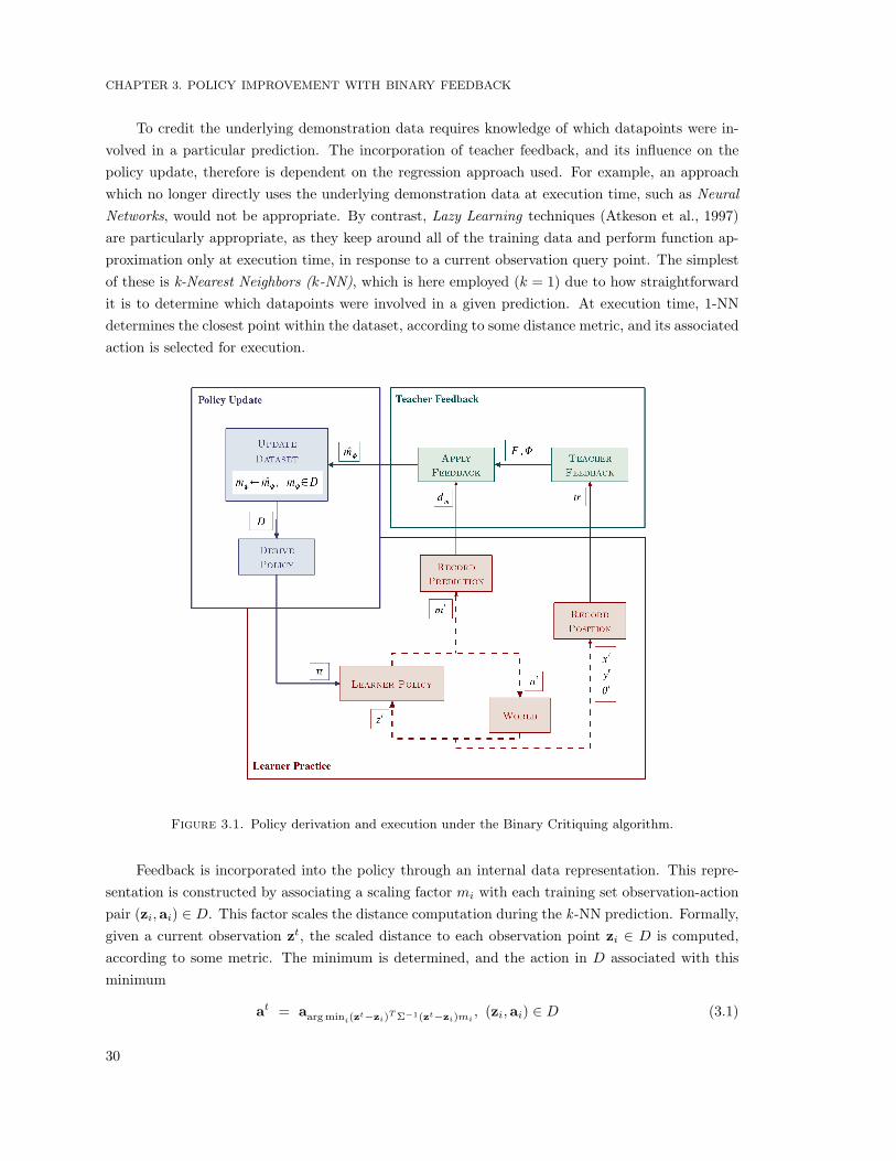
CHAPTER 3. POLICY IMPROVEMENT WITH BINARY FEEDBACK
To credit the underlying demonstration data requires knowledge of which datapoints were in-volved in a particular prediction. The incorporation of teacher feedback, and its influence on thepolicy update, therefore is dependent on the regression approach used. For example, an approachwhich no longer directly uses the underlying demonstration data at execution time, such as NeuralNetworks, would not be appropriate. By contrast, Lazy Learning techniques (Atkeson et al., 1997)are particularly appropriate, as they keep around all of the training data and perform function ap-proximation only at execution time, in response to a current observation query point. The simplestof these is k-Nearest Neighbors (k-NN), which is here employed (k = 1) due to how straightforwardit is to determine which datapoints were involved in a given prediction. At execution time, 1-NNdetermines the closest point within the dataset, according to some distance metric, and its associatedaction is selected for execution.
Figure 3.1. Policy derivation and execution under the Binary Critiquing algorithm.
Feedback is incorporated into the policy through an internal data representation. This repre-sentation is constructed by associating a scaling factor mi with each training set observation-actionpair (zi,ai) ∈ D. This factor scales the distance computation during the k -NN prediction. Formally,given a current observation zt, the scaled distance to each observation point zi ∈ D is computed,according to some metric. The minimum is determined, and the action in D associated with thisminimum
at = aarg mini(zt−zi)
TΣ−1(zt−zi)mi, (zi,ai) ∈ D (3.1)
30

3.1 ALGORITHM: BINARY CRITIQUING
is executed. In our implementation the distance metric is Euclidean and observation dimensions arescaled inversely with the range of the demonstration dataset within the diagonal matrix Σ−1. Thevalues mi are initially set to 1.
Figure 3.1 presents a schematic of this approach. Unlike the other algorithms of this thesis,including the baseline feedback algorithm (Fig. 2.4), here only the metrics used to compute thepolicy prediction are recorded, and not the executed observation-action pairs. The reason is due tothe manner of feedback incorporation into the policy. To incorporate feedback, the scaling factorassociated with the dataset point that provided the action prediction is updated, as shown within theUpdate Dataset box within the schematic. Only the scaling factor, and not the observation-actionpair, therefore needs to be recorded.
3.1.2. Algorithm Execution
Algorithm 2 presents pseudo-code for the BC algorithm. This algorithm is founded on thebaseline feedback algorithm of Chapter 2 (Alg. 1). In addition to the contents of the recordedprediction trace, the distinguishing details of BC lie in the type and application of teacher feedback(Alg. 1, lines 17-18).
The teacher demonstration phase produces an initial dataset D, and since this is identical to thedemonstration phase of the baseline feedback algorithm (Alg. 1, lines 1-8), for brevity the details ofteacher execution are omitted here. The learner execution portion of the practice phase also proceedssimilarly the baseline algorithm. The difference lies in what is recorded into the prediction trace dm;here the scaling factor mt = mi of the dataset point that provided the prediction is recorded, alongwith its distance to the query point `t ≡ (zt − zi)
T Σ−1 (zt − zi) (line 8).
Algorithm 2 Binary Critiquing
1: Given D2: initialize π ← policyDerivation(D)3: while practicing do4: initialize d← {}, tr ← {}5: repeat6: predict { at, `t,mt } ← π (zt)7: execute at
8: record dm ← dm ∪ (`t,mt) , tr ← tr ∪ (xt, yt, θt)9: until done
10: advise { c,Φ } ← teacherFeedback( tr )11: for all ϕ ∈ Φ, (`ϕ,mϕ) ∈ dm do12: replace mϕ ← mϕ + κ
`ϕ , mϕ ∈ D
13: end for14: rederive π ← policyDerivation(D)15: end while16: return π
Teacher feedback (line 10) under the BC algorithm proceeds as follows. For each learner exe-cution, the teacher selects segment Φ, dΦ ⊆ d, of the trajectory to flag as poorly performing. The
31

CHAPTER 3. POLICY IMPROVEMENT WITH BINARY FEEDBACK
teacher feedback is a negative credit c ≡ z (Sec. 2.4.2), a binary flag indicating poor performance.This credit will be associated with all selected points.
The teacher feedback is then applied across all data recorded in dm and within the indicatedsubset Φ (line 12). For each selected execution point in dm, indexed as ϕ ∈ Φ, the value mϕ ofthis point is increased according to line 12, where κ > 0 is some empirically determined constant(here κ = 0.1). The amount by which mϕ is increased is scaled inversely with distance `ϕ so thatpoints are not unjustly penalized if, due to sparsity in D, they provide recommendations in distantareas of the observation space which they do not support. To update mϕ in this manner means thatdatapoints whose recommendations gave poor results (according to the critique of the teacher) willbe seen as further away during subsequent k -NN distance calculations.
These details of the dataset update are the real key to critique incorporation. To then incor-porate the teacher feedback into the learner policy simply consists of rederiving the policy from thedataset D, now containing the updated values of m (line 14).
3.2. Empirical Implementation
This section presents the details and results of applying the BC algorithm to a simulated motioninterception task. Policy performance was found to improve with critiquing, and furthermore toexceed the performance of the demonstration policy (Argall et al., 2007a).
3.2.1. Experimental Setup
Empirical validation of the BC algorithm is performed within a simulated motion interceptiondomain. First presented are the task and domain, followed by the details of demonstration andcritiquing, and lastly the evaluation measures.
3.2.1.1. Simulated Motion Interception Task and Domain. Within these experi-ments, a simulated differential drive robot is tasked with intercepting a moving ball (Fig. 3.2). Sincea differential drive robot may only drive forward or turn, and cannot go sideways, interception of amoving object becomes a difficult task. The task also depends heavily on the dynamics of the world,and so writing an appropriate control policy can be challenging in the absence of accurate predictiveworld motion models.
Care was taken to keep the simulated domain realistic to the real world domain of a SegwayRMP robot. The robot is assumed to use a differential-drive mechanism, with a low-level controllerthat takes desired robot speeds as input commands. For the robot, motion is propagated by simpledifferential drive simulation of the global robot position
xt+1 = xt + vt cos(θt)
yt+1 = yt + vt sin(θt)
θt+1 = θt + ωt · dt
(3.2)
where (x, y) is the global robot location and θ the global orientation. Dynamic limitations on the per-formance of the robot constrain its linear and rotational speeds (v ∈ [0.0, 2.0]ms , ω ∈ [−3.0, 3.0] rads )
32

3.2 EMPIRICAL IMPLEMENTATION
Figure 3.2. Simulated robot motion (left) and ball interception task (right).
and accelerations (v ∈ [0.0, 3.0]ms , ω ∈ [−7.0, 7.0] rads ). For the ball, motion is propagated by aconstant velocity model with a simple exponential decay on initial velocity to mimic frictional loss,
xt+1B = xtB + γtxtBdt
yt+1B = ytB + γtytBdt
(3.3)
where γ ∈ [0, 1] is the decay constant (here γ = 0.99). Initial ball velocity is limited (‖x0B , y
0B‖ ∈
[−2.5, 0.0]ms ). The positions generated within the domain are bounded above and below (x, y ∈[0.0, 5.0]m), constraining both the ball and the robot locations.
3.2.1.2. Demonstrations, Observations and Learner Practice. Teacher demonstra-tions are performed via teleoperation of the robot by a hand-written suboptimal controller able toselect changes in rotational and translational speed. This teacher was chosen for two reasons: thefirst being to highlight the ability of this algorithm to improve upon teacher suboptimality, and thesecond because of the ease with which a large number of demonstrations could be provided (here100). For teacher demonstrations, initial world configurations are uniformly sampled from the rangeof world locations (x, y) ∼ U (0.0, 5.0m) and ball speeds (x, y) ∼ U
(−2.5, 0.0ms
).
Learner policy executions begin from an initial world configuration of robot-relative ball positionand velocity. Execution ends when the robot either intercepts the ball or the ball travels out ofbounds. During execution the robot may directly observe its own position and the ball position,as shown in Figure 3.3. Let (dtb, φ
tb) be the distance and angle to the ball in the robot-relative
frame, and (dt, φt) the distance traveled by and heading of the robot within the global world frame.The observations computed by the robot are 6-dimensional: [dtb, φ
tb, (d
tb − d
t−1b ), (φtb − φ
t−1b ), (dt −
dt−1), (φt−φt−1)]. The actions predicted by the robot are 2-dimensional: change in rotational speed(∆v) and change in translational speed (∆ω).
33

CHAPTER 3. POLICY IMPROVEMENT WITH BINARY FEEDBACK
Figure 3.3. World state observations for the motion interception task.
An example cycle of learner execution and teacher critique, along with the subsequent improve-ment in learner execution, is demonstrated in Figure 3.4. Blue and red lines mark respectively therobot and ball execution paths on the ground plane, arrow heads indicate direction of travel, andthe red circle is a distance threshold on successful interception. In this example the robot doesinitially intercept the ball, but the loop in its trajectory is inefficient (A). The teacher critiques thistrajectory, flagging the loop as an area of poor performance (B). The robot repeats the execution,now without the inefficient loop (C).
3.2.1.3. Evaluation. To measure the performance of this algorithm, trajectory executionsare evaluated for success and efficiency. A successful interception is defined by (a) the relativedistance to the ball falling below some threshold ε and (b) the ball and robot both remaining withinbounds (ε = 0.01m). Efficiency is measured by execution duration, with trajectories of shorterduration being considered more efficient.
Performance evaluations occur on an independent test set containing nt initial world conditionsrandomly sampled from a uniform distribution within the bounds of the training set (nt = 100).A practice run is defined as execution from a single randomly sampled initial world condition (notfound within the test set), followed by teacher feedback and optional re-execution, at the teacher’sdiscretion. To mark learner progress, execution on the test set is carried out after every np practiceruns (np = 20, 120 runs in total). Practice runs conclude when no further performance improvementis observed on the test set. Note that during the test evaluations, the learner executes using its mostrecent policy π, and no teacher critiquing or policy updating occurs. For comparative purposes, theperformance of the demonstration policy on this test set is evaluated as well.
3.2.2. Results
In this section we show learner performance to improve with critiquing. This performanceimprovement is demonstrated through an increase in interception successes, as well as more efficient
34
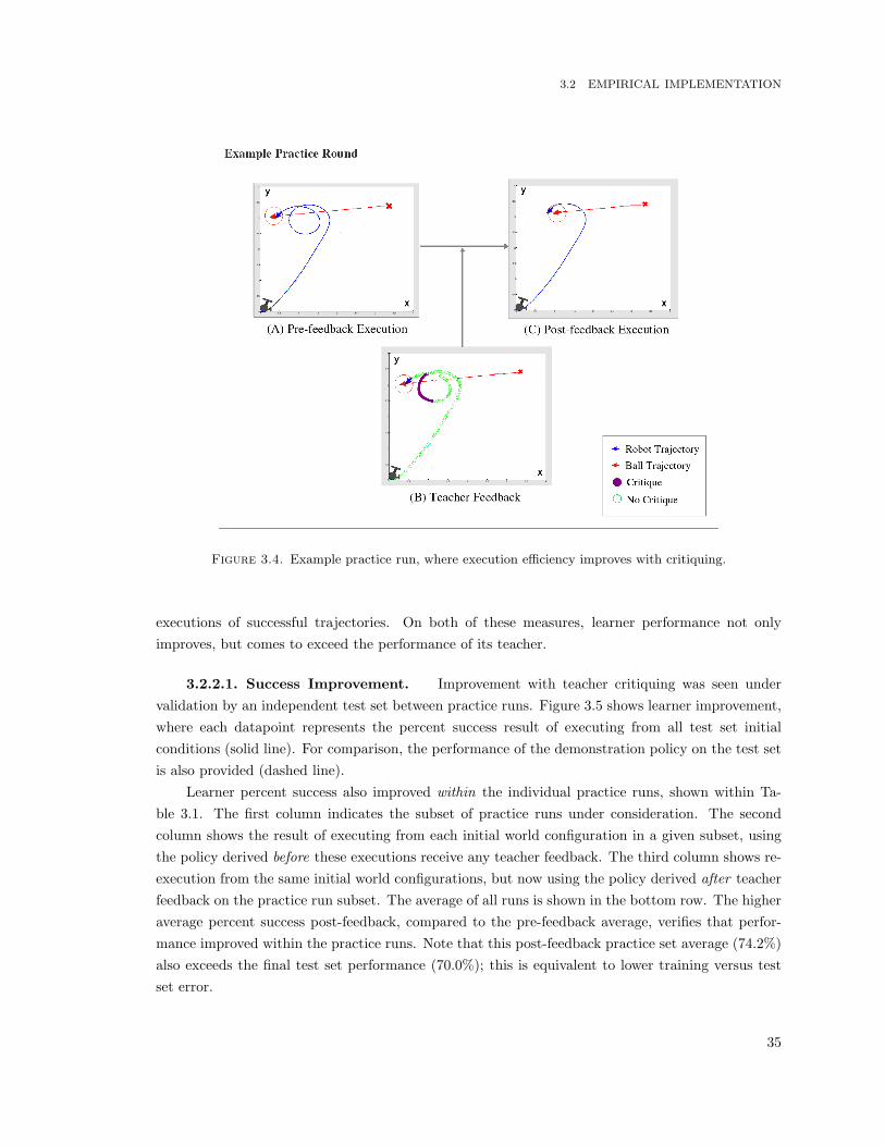
3.2 EMPIRICAL IMPLEMENTATION
Figure 3.4. Example practice run, where execution efficiency improves with critiquing.
executions of successful trajectories. On both of these measures, learner performance not onlyimproves, but comes to exceed the performance of its teacher.
3.2.2.1. Success Improvement. Improvement with teacher critiquing was seen undervalidation by an independent test set between practice runs. Figure 3.5 shows learner improvement,where each datapoint represents the percent success result of executing from all test set initialconditions (solid line). For comparison, the performance of the demonstration policy on the test setis also provided (dashed line).
Learner percent success also improved within the individual practice runs, shown within Ta-ble 3.1. The first column indicates the subset of practice runs under consideration. The secondcolumn shows the result of executing from each initial world configuration in a given subset, usingthe policy derived before these executions receive any teacher feedback. The third column shows re-execution from the same initial world configurations, but now using the policy derived after teacherfeedback on the practice run subset. The average of all runs is shown in the bottom row. The higheraverage percent success post-feedback, compared to the pre-feedback average, verifies that perfor-mance improved within the practice runs. Note that this post-feedback practice set average (74.2%)also exceeds the final test set performance (70.0%); this is equivalent to lower training versus testset error.
35

CHAPTER 3. POLICY IMPROVEMENT WITH BINARY FEEDBACK
Test Set Percent Success
Figure 3.5. Improvement in successful interceptions, test set.
Practice Run Success, Pre-feedback π (%) Success, Post-feedback π (% )1-20 65 8021-40 60 7541-60 50 5561-80 50 6081-100 65 90101-120 75 85
All 60.83 74.17
Table 3.1. Pre- and post-feedback interception percent success, practice set.
3.2.2.2. Efficiency Improvement. Negative feedback was also found to improve learnerexecution efficiency. That is, the robot learned to intercept the ball faster, indicated by reducedexecution times. Efficiency results on the independent test set, from the learner executing with itsinitial and final policies, are presented in Table 3.2. Note that to decouple this measure from success,only those runs in which all policies were successful are compared (since the out-of-bounds successmeasure otherwise taints the comparison, given that from identical starting conditions a successfulinterception is necessarily faster than a unsuccessful one). Again, for comparison, results from thedemonstration policy test set executions are also provided.
Learner Initial π Learner Final π TeacherSuccess % 56 70 62
Execution Time (s) 2.73 1.96 2.87
Table 3.2. Interception task success and efficiency, test set.
36

3.3 DISCUSSION
3.3. Discussion
A discussion of the BC algorithm and the above empirical implementation is presented in thissection. To begin, the conclusions of this work are detailed, followed by a discussion of futuredirections for the BC algorithm.
3.3.1. Conclusions
This section highlights some noteworthy conclusions which may be drawn from this empiricalimplementation of the BC algorithm. First discussed is the unexpected extent of policy improvementwith critiquing, which enabled performance beyond that of the demonstration teacher. Next insightsinto the benefit of providing critique feedback with a human teacher are discussed.
3.3.1.1. Improvement Beyond Teacher. The empirical results show that the learnerpolicy, through the incorporation of teacher feedback, was able to perform better than the demon-strator (Fig. 3.5, Tbl. 3.2). These results underline the benefits of using the BC algorithm in thisexperimental setup. The hand-coded demonstration controller was not optimal for the domain. Bycritiquing the robot’s executions, the algorithm was able to correct for some demonstration error,thus improving the robot’s performance beyond the capabilities of the demonstration teacher, andall in a simple and straightforward manner. The BC approach thus is shown to address the LfDlimitation of suboptimal teacher demonstrations.
3.3.1.2. Providing Critique Feedback. Feedback provided in this implementation ofthe BC algorithm depended on human-expertise. The evaluation criteria used by the feedbackteacher was a combination of ball interception success and execution efficiency. To define metricsthat capture these criteria is straightforward, for example those defined for analytical purposes inSection 3.2.1.3. Were only such simple metrics encoded within the feedback, a critiquing teachercould easily be automated.
A critique does not simply provide an overall measure of execution performance, however.Critiques additionally indicate areas that contributed to the poor values of these evaluation metrics.For example, consider the execution of Figure 3.4. Being able to assess that an execution is onthe whole inefficient, versus being able to determine which portions of the execution caused theinefficiency, are two very different tasks.
In contrast to overall task performance, to formally define a metric for credit assignment, thatindicates source areas for poor performance, can be quite difficult. This challenge is similar to themuch explored issue of reward back-propagation within the field of Reinforcement Learning. TheBC algorithm circumvents this issue by exploiting a human for the task of credit assignment, thusunderlining the worth in having a human feedback teacher in this algorithm.
3.3.2. Future Directions
Here two key areas for the extension of the BC algorithm are identified. The first addresses thepotential for critique over-application and the option for real-valued feedback. The second discussesproviding human feedback that contains more information than just a binary performance flag.
37

CHAPTER 3. POLICY IMPROVEMENT WITH BINARY FEEDBACK
3.3.2.1. Directional Critiques. One weakness of this algorithm is that points in D mightbe unduly penalized by critiquing, since where query points are in relation to training datapointsis not considered when updating scaling factor m. Consider two query points located at identicaldistances, but orthogonal directions with respect, to a given training point. The training point’srecommended action might be appropriate for one query point but not the other. If so, actionexecution would incur different success for each query point, and therefore also conflicting feedback.The incorporation of query point orientation into the update of m is thus a potential improvementfor this algorithm. A similar approach is taken in the work of Bentivegna (2004), where state-action-query Q-values are considered in a k -NN policy derivation, and are updated based on learnerexecution performance.
Another extension to the BC algorithm could incorporate real-valued feedback. Under thecurrent formulation, critiques provide a binary poor performance flag. The incorporation of thisfeedback into the policy, through an update of the scaling factor m, does depend on the relativedistance between the query and dataset points. However, this incorporation could further dependon the value of a critique, if the feedback were not binary. In this case, larger critique values couldaffect larger increases to the scaling factor m. For example, real-valued feedback could be a functionof performance metrics, like the success and efficiency metrics defined for this domain (Sec. 3.2.1.3).
3.3.2.2. More Informative Feedback. Providing a binary critique, like providing RLreward, gives the learner an indication of where poor action selection occurred. It does not, however,provide any sort of indication about what should have occurred instead. The only way to determinewhich action would produce a superior performance is to revisit the state and execute a differentaction. Such an approach easily becomes intractable on real robot systems operating in worlds ofinfinite state-action combinations.
Furthermore, under a LfD paradigm, any exploratory actions taken by the learner are restrictedto either those that were demonstrated by the teacher, or those that possibly result from regressiongeneralization. Note however that generalized actions only result from certain regression techniques,for example those that produce a soft average over dataset actions (e.g. kernelized averaging) but notthose that strictly select a single dataset action (e.g. 1-NN). If a desired action was not demonstratedby the teacher, possible reasons are that during demonstration the teacher never visited a state inwhich taking this action was appropriate, or that the teacher did visit such a state but the teacheris suboptimal. Regardless of the reason, it is possible that the learner does not even have access toa better action for an execution state that received a poor performance critique.
We posit that more informative, corrective, feedback would prove useful to the learner. Fur-thermore, feedback that expands the set of available actions beyond those contained within thedemonstration set should also improve policy performance. The development of our advice-operatorfeedback technique, introduced in the following chapter, is grounded on both of these considerations.
3.4. Summary
Binary Critiquing (BC) has been introduced as an algorithm that credits policy performancewith teacher feedback in the form of binary performance flags. The teacher selects poorly performing
38

3.4 SUMMARY
portions of a learner execution to receive the binary credit, thus overcoming the issue of credit assign-ment common in many reward-based feedback algorithms. The learner uses the crediting feedbackto update its policy; in particular, the feedback is used to modify how the underlying demonstrationdata is treated by the policy derivation technique. By thus weighting the demonstration datapointsaccording to their relative performance, the robot is able to improve its policy.
The BC algorithm was implemented within a simulated robot motion interception domain.Empirical results showed improvements in success and efficiency as a consequence of the creditingfeedback. Interestingly, the performance of the final learned policy exceeded the performance of thedemonstration policy, without modifying the contents of the demonstration dataset.
There are many benefits to using a human for credit assignment. Within the BC algorithmparticularly, the human selects portions of an execution to flag as poorly performing. Rather thanjust crediting poor performance where it occurs, segment selection allows for behaviors that leadto poor performance to receive negative credit as well. Furthermore, since a human evaluates theexecution, the robot is not required to be able to detect or measure the aspects of an executionthat define poor performance. A human evaluator also allows for the option of evaluation metricsthat are perhaps too subtle, or complex to be detected and represented computationally, within thelearning system.
Future research directions for the BC algorithm were identified to included directional critiquesthat consider query point orientation, and real-valued critiques that impart a measure of relativerather than just binary performance. Feedback that is corrective was also identified as a promisingdirection for future work, motivating the development of our corrective advice-operator technique,introduced in the following chapter.
39

CHAPTER 4
Advice-Operators
The ability to improve a policy from learner experience is useful for policy development, and onevery direct approach to policy improvement is to provide corrections on a policy execution.
Corrections do not require any exploration on the part of the learner, since the preferred action totake, or state to enter, is explicitly indicated. When provided by a human, corrections additionallydo not require that any automatic policy evaluations be performed by the robot learner or by thelearning system as a whole.
The work of this thesis focuses on low-level robot motion control within continuous action-spaces. To indicate a preferred action or state within continuous state-action spaces requires pro-viding a continuous-valued correction. While a human teacher may have a general idea of how tocorrect the behavior, expecting her to know the appropriate continuous value that corrects an ex-ecution point is neither reasonable nor efficient. For example, a human teacher may know that anexecution should have been faster, but not that the speed should have been exactly 2.3ms insteadof 2.1ms . Furthermore, since our motion control policies are sampled rapidly, e.g. at 30Hz, anyexecuted robot behavior deemed by the human to need correcting likely endured over multiple exe-cution points. Continuous-valued corrections therefore must be provided for all of these points, thusfurther increasing the burden on the teacher. With our contributed correction approach, we aim tocircumvent both of these difficulties.
This chapter introduces advice-operators as a language through which a human teacher providescorrections to a robot student. Advice-operators perform mathematical computations on continuous-valued datapoints. To provide a correction, the teacher selects from a finite list of advice-operators.The robot learner applies the operator to an execution datapoint, modifying its value and producing acontinuous-valued correction. Paired with the segment selection approach of our feedback framework(Ch. 2), an operator is applied over all of the execution points within the segment. The selection ofa single piece of advice and application segment therefore provides continuous-valued corrections onmultiple execution points. In this manner, our approach enables correction-giving that is reasonablefor a human to perform, even within our continuous-valued, rapidly sampled, domain.
While advice-operators significantly simplify the process of providing continuous-valued correc-tions, the operators themselves still must be defined. In this chapter we additionally contribute a
CHAPTER 4. ADVICE-OPERATORS
principled approach to the development of action advice-operators. We will employ this developmentapproach within later chapters of this thesis.
We also present in this chapter a comparison of the data produced through the techniques ofexclusively demonstration versus advice-operators, since one motivation for the formulation of ourpolicy corrections within a LfD framework is to provide an alternative to teacher demonstrations.Common limitations to LfD datasets include poor teacher-learner correspondence and suboptimalteacher performance, neither of which may be addressed by providing more teacher demonstrations.We show the two techniques to produce data that exists in different areas of the state and actionspace, and furthermore establish advice-operators as an effective approach for policy improvementthat produces smaller datasets in addition to superior performance.
This chapter begins with an overview of advice-operators. In Section 4.2 our principled approachto the development of action advice-operators is detailed. Section 4.3 then presents a comparison be-tween data produced from teacher feedback and more demonstration. Directions for future researchare identified in Section 4.4.
4.1. Overview
This section introduces our approach to correcting policies within continuous state-actionspaces. We begin with a description of our correction technique, followed by a delineation of somerequirements for the application of this technique.
4.1.1. Definition
To address the challenge of providing continuous-valued corrections, we introduce advice-operatorsas a language through which a human teacher provides policy corrections to a robot student. Con-cretely defined, an advice-operator is a mathematical computation performed on an observationinput or action output. Key characteristics of advice-operators are that they:
• Perform mathematical computations on datapoints.
• Are defined commonly between the student and advisor.
• May be applied to observations or actions.
To illustrate with an example, consider a simple operator that modifies translational accelerationby a static amount δ. Suppose this operator is indicated, along with a segment of 15 execution datapoints. The translational speed a0 of executed point 0 then updates to a0 ← a0 + δ, point 1 toa1 ← a1 + δ, and so forth until point 14 updates to a14 ← a14 + δ.
4.1.2. Requirements for Development
Advice-operators perform mathematical computations on the observations or actions of execu-tion datapoints. To develop advice-operators requires that the designer be able to isolate specificelements of a datapoint formulation as responsible for producing the particular behavior that willbe corrected by the operator. The majority of the operators developed and used in the work ofthis thesis are action-modifying operators; this consideration is discussed further in Section 4.4.2.
42

4.2 A PRINCIPLED APPROACH TO ADVICE-OPERATOR DEVELOPMENT
We therefore restrict this discussion of advice-operator development to action-modifying operators,while noting that a parallel, though not necessarily equivalent, discussion exists for the developmentof observation-modifying operators.
Within this action context, to isolate the necessary datapoint elements involves identificationof the component actions that are responsible for producing the particular aspect of the net actionthat the operator is intended to correct. For example, if a net action involves both rotationaland translational speeds, to develop an operator that increases linear velocity involves isolatingthe translational speed component of the net action. An appropriate modification for this isolatedelement, that produces the desired behavior change, is then additionally required; namely, thatincreasing the translational speed will result in the desired modification of increased linear velocity.
Advice-operator development depends generally on the capabilities of the robot, and specificallyon the state-action space of the task at hand. The generality of an operator - that is, its applicabilityto more than one task - depends on design decisions made by the developer. Many valid formulationsfor how to develop advice-operators potentially exist, the most straightforward of which is to developeach operator by hand and without generality to other tasks. Advice-operator development underour approach, presented in the following section, produces operators that are as general as thedefined actions. That is, for task-specific actions, task-specific operators will result. For actionsgeneral to the robot, general advice-operators will result. Actions common to multiple tasks on therobot therefore are able to share advice-operators developed under our technique.
4.2. A Principled Approach to Advice-Operator Development
This section contributes our principled approach to the development of action advice-operators.We first define a set of baseline advice-operators, followed by a technique for building new operatorsthrough the scaffolding of existing operators. The section concludes with a presentation of constraintsimposed on the system to keep the synthesized data firmly grounded within the robot’s capabilities.
4.2.1. Baseline Advice-Operators
Advice-operator development under our approach begins with the definition of a baseline setof advice-operators. For multi-dimensional action predictions, e.g. a 2-D prediction consisting ofrotational speed and translational speed, the baseline operators are defined for each single actiondimension, and function as first and second order modifications to the value of that action dimension.Concretely, given a recorded observation-action execution trace d and selection Φ, such that subsetdΦ ⊆ d contains executed action ai ∈ dΦ (of a single action dimension), the baseline operators are:
• Static: A static modification amount δ, applied equally across all selected points, producingaction ai ← ai + δ.
• Fractional : A fractional modification amount α, that operates on the executed actionvalues ai ∈ dΦ, producing action ai ← ai + αai.
43
CHAPTER 4. ADVICE-OPERATORS
• Incremental Fractional : Fractional modification amounts i|Φ|β, that operate as linearly in-
creasing fractional modification amounts on the executed action values ai ∈ dΦ, producingactions ai ← ai + i
|Φ|βai.
Here |Φ| is the size of the selected segment, i = 1 . . . |Φ| and δ > 0, α > 0, β > 0 are all constantparameters. Each operator furthermore takes a binary parameter, indicating a positive or negativemodification amount.
The first operator Static allows for the static augmentation of an action value, particularlyuseful if the value was previously zero or of opposite sign to the desired value. The second operatorFractional enables augmentations that increase or decrease according to the size of the executedaction value, which is useful for producing smooth changes as well as very large or very smallmodification amounts. The reasoning behind the final operator Incremental Fractional is to allowincremental easing into a modification. For example, in the case of ten selected actions a1, a2 . . . a10 ∈dΦ, this operator adds β
10a1 to the first action and 2β10 a2 to the second action, up to the addition of
βa10 to the final action in the set. At first glance, this may appear to represent an “acceleration”across the executed points added to the dataset. Careful to note, however, is that points are treatedindividually by the regression techniques and no notion of execution trace or sequence is taken intoaccount once points have been added to the demonstration set. The only difference between thisoperator (Incremental Fractional) and the second operator (Fractional) therefore is that smallermodifications are made to earlier points, and larger modifications to later points, along the selectedexecution segment.
For the experimental implementations of the following chapters, the parameter values are set asα = 1
3 and β = 12 . Section 4.2.3.1 describes how to set δ. The three baseline operators are developed
for each of two single actions, translational and rotational speed, resulting in six baseline operators.Note that these operators are specific to motion control on our differential drive robot in general,and not to any particular motion task.
4.2.2. Scaffolding Advice-Operators
Advice-operator development continues with the definition of more complex operators. In par-ticular, these operators are built, or scaffolded, from existing operators, beginning with the baselineset. Our approach provides an interface through which existing advice-operators are composed andsequenced into more complex operators.
The advice-operator building interface functions as follows. First the existing children operatorsthat will contribute to the new parent operator are selected. Second, the range over which eachoperator will be applied is indicated. This allows for flexibility in the duration of the contributingoperators, such that a given child operator is applied over only a portion of the execution segmentif desired. For adaptability to any segment size, application range is indicated by a percentage,e.g. a range of 25 → 50% indicates the second quarter of a segment. Figure 4.1 presents anexample applicability scenario where one contributing operator (Fractional Translational Speed) hasan associated range of 0 → 75% and thus is applied over the first three-quarters of the execution
44

4.2 A PRINCIPLED APPROACH TO ADVICE-OPERATOR DEVELOPMENT
segment, and a second contributing operator (Static Rotational Speed) has a range of 50 → 100%and thus is applied over the final half of the segment.
Figure 4.1. Example applicability range of contributing advice-operators.
In the third step, the parameters for the new operator are specified. To define a parameterfor the parent operator, a single parameter is selected from the parameter list of each contributingchild operator. The new parameter combination across all children is given a name, and this set nowconstitutes a single new parameter for the parent operator. Another parameter combination maythen be specified, as per the intents of the designer; the only limit on the number of parameters thatmay be associated with a given operator is the number of unique combinations of child parameters.The new operator is then added to the operator list and available for immediate use.
Upon application, selecting this new operator and one of its parameters triggers an applicationhierarchy. The hierarchy begins with the application of each indicated child operator, over theexecution segment subset indicated by the application range of the child operator, and with theparameter specified within the selected parent parameter combination. If a given child operatoris not itself a baseline operator, it too is defined by a set of children operators and its associatedparameter specifies a parameter combination for these children; these children also are applied overthe segment. This process continues until all operators under consideration are baseline operators,whose application is mathematically defined as described in Section 4.2.1.
To illustrate this building interface, consider the development of an operator named AdjustTurn, outlined in Figure 4.2. In step one the contributing child operators are selected. Two operatorsare indicated: the Fractional operator for the rotational speed action, and the Fractional operatorfor the translational speed action. In step two the applicability range of each child operator isindicated; here both operators are applicable over the entire execution segment (0 → 100% of thesegment). In step three, parameters for the new operator are specified. The first parameter specified,named tighten, sets the parameter for the rotational speed Fractional operator as increase and thetranslational speed Fractional operator as decrease. The second parameter specified, named loosen,sets the parameter for the rotational speed Fractional operator as decrease and the translationalspeed Fractional operator as increase. The overall functioning of the new operator is to tighten a
45

CHAPTER 4. ADVICE-OPERATORS
turn by increasing rotational speed and decreasing translational speed, or alternately to loosen aturn by decreasing rotational speed and increasing translational speed.
Figure 4.2. Advice-operator building interface, illustrated through an example (buildingthe operator Adjust Turn).
In summary, advice-operators are built as a hierarchy, or tree, of existing operators. Selectionof an operator triggers a sequence of calls to underlying operators. The leaf nodes of this tree are thebaseline operators, whose functioning is specified by the basic hand-written mathematical functionsdescribed in the previous section. The mathematical functioning of all non-baseline operators thusresults from the sequencing and composition of functions built from the baseline mathematics.
4.2.3. The Formulation of Synthesized Data
The data modification techniques presented here amount to data synthesis from learner exe-cutions and teacher advice. This synthesis is subject to multiple constraints intended to producesynthesized data that is firmly grounded on both the underlying learner execution and the physicalcapabilities of the robot. Furthermore, steps are taken to ensure that data that corrects iterativepolicies does not negatively impact the final policy behavior.
4.2.3.1. Constraining Corrections. Beyond being a function of executed action values,the modification amounts produced by advice-operators are further tied to the physical constraintsof the robot. In particular, assuming a standard acceleration value of ν, the static modificationamount δ of operator Static is defined as νdt, where dt is the execution framerate.1 Our systemsruns at 30Hz, and thus dt = 0.033s.
1If a standard acceleration value is not defined for the robot system, another reasonable option for this value may be
selected, for example average acceleration.
46
4.2 A PRINCIPLED APPROACH TO ADVICE-OPERATOR DEVELOPMENT
The final advice-modified action is additionally constrained to lie within an amount η of theexecuted action value. This constrains the synthesized points to lie near points that were actuallyexecuted, and thus near the capabilities of the existing demonstration set from which the policy thatproduced this execution was derived. In particular, assuming a maximum acceleration value of νmx,the constraining amount η is defined as νmxdt, where dt again is the execution framerate.2 Thistheoretically guarantees that the advice-modified datapoint is reachable from the executed pointwithin 1-timestep.
4.2.3.2. Addressing Suboptimal Iterative Data. One consequence of constraining mod-ifications in this manner is that the mapping represented by the synthesized data might not beconsistent with the behavior desired of the final policy. This is because the synthesized data isconstrained to lie near the learner execution, which, given that the execution was corrected, presum-ably was not consistent with the final desired behavior. Though the corrected, synthesized mappingdoes represent an iterative improvement on the mapping exhibited by the learner execution, thiscorrected mapping may still conflict with the desired behavior of the final policy. If the correctedmapping does not match the behavior desired of the final policy, the synthesized data equates toa suboptimal demonstration of the final policy behavior. Like any suboptimal demonstration, thisdata will degrade policy performance.
As an illustration, consider a learner executed translational speed, 1.2ms , that is much slowerthan the target behavior speed, 2.5ms , and a constrained modification amount of 0.3ms . A step in thedirection of the target speed produces an advice-modified action with value 1.5ms ; to add this datato the demonstration set equates to providing a demonstration at speed 1.5ms . While this action isan improvement on the learner executed speed, it is suboptimal with respect to the target behaviorspeed of 2.5ms . The addition of this datapoint to the demonstration set thus amounts to providingthe final policy with a suboptimal demonstration.
To circumvent this complication, our approach augments the state observation formulationwith internal observations of the current action values. This anchors the action predictions of thestate-action mapping to the current observed action values. Mappings now represent good behaviorgiven the current action values, and thus will not conflict with the final policy even if they are notgood demonstrations of the target behavior. Returning to our illustration, under this formulationthe speed 1.5ms will be considered an appropriate prediction only when the current speed is 1.2ms .Should the learner later revisit that area of the world with a speed of 2.0ms , for example, the policywill not attempt to slow the learner down to 1.5ms .
The benefit of this observation formulation is more robust and flexible advice-giving, since advicethat improves the behavior of an iterative policy, but is suboptimal for the final policy, is no longera hazard. A drawback is that this observation formulation increases the observation-space, whichtypically correlates to slower learning times and the need for more training data. An alternativesolution could be to incorporate LfD techniques that explicitly address suboptimal demonstrationdata, though to date few such techniques exist (see Ch. 9).
2The maximum acceleration value νmx may be defined either by the physical constraints of the robot or artificially
by the control system.
47
CHAPTER 4. ADVICE-OPERATORS
4.3. Comparison to More Mapping Examples
In this section we present a comparison of data produced from the advice-operator techniqueagainst data produced from more teacher demonstrations. In both cases, an initial dataset is pro-duced from demonstration, and an initial policy is derived from this dataset. Data produced underthe feedback technique is then synthesized from learner executions with its current policy and teachercorrections on these executions. Data from more-demonstrations is produced in the same manner asthe initial dataset, namely teacher demonstration, but the demonstrations are provided in responseto learner executions with its current policy. To begin, we compare the distribution of data withinthe observation and action spaces, as produced under each technique. We next compare the qualityof the resultant datasets, as measured by dataset size and the relative performance of policies derivedfrom the respective datasets.
4.3.1. Population of the Dataset
The work presented in this section compares two datasets: one built using our feedback tech-niques, and one built from demonstration exclusively. Both datasets are seeded initially with thesame demonstration data, since all of our feedback algorithms rely on an initial policy derived fromdemonstration. As the learner executes, the teacher observes the learner performance and offerscorrective feedback, in the case of the feedback dataset, or more teleoperation demonstrations, in thecase of the more-demonstration dataset. Note that the feedback provided by the teacher includesadvice-operators as well as positive credit (Sec. 2.3.1.1), which equivalently may be viewed as anidentity function advice-operator that leaves a datapoint unchanged. The actual task that producedthe data of this section is presented in Chapter 6 (building the primitive policy datasets); the detailsof the task are tangential to the focus of the discussion here.
Figure 4.3 provides a comparison of the distribution of new data within the observation space.This histogram presents the distance between dataset observations and the observation of a newpoint being added to that dataset, gathered across multiple new datapoints (1, 239 for feedback,2, 520 for more-teleoperation). Along the horizontal axis is the Euclidean 1-NN distance betweena new datapoint and the existing dataset, i.e. the distance to the single closest point within thedataset, and along the vertical axis is the relative (fractional) frequency count of a given 1-NNdistance value. The most notable difference between the data derived from more demonstration andthat derived from feedback lies in the smaller distance values. The more-demonstration approachmore frequently provides new data that is close (≤ 0.05) to the existing dataset. Furthermore,when comparing the mean and standard deviation of the distribution of 1-NN distances, the more-teleoperation distribution has a lower mean and larger standard deviation (0.15 ± 0.14) than thefeedback distribution (0.21± 0.02).
These observation space results suggest that our feedback techniques take larger steps away fromthe initial demonstration dataset, into more remote areas of the observation space. It is possible thatthe demonstration approach also visits these areas, but over more, smaller step, iterations. Given theperformance results presented in the following section however (Sec. 4.3.2), the more likely possibilityis that there are observation areas which are unvisited by the teacher during demonstration, but
48

4.3 COMPARISON TO MORE MAPPING EXAMPLES
Distance between New and Existing DataWithin the Observation Space
Figure 4.3. Distribution of observation-space distances between newly added datapointsand the nearest point within the existing dataset (histogram).
which are visited by the learner executions and added after advice-modification to the feedbackdataset. One possible explanation for an absence of teacher demonstrations in particular observation-space areas is a lack of knowledge on the part of the teacher that demonstration is needed in theseareas. Another explanation is that the particular execution technique of the teacher does visit theseobservation-space areas, or perhaps that limitations in the mechanism employed for demonstrationcomplicate access to these areas; both of these explanations indicate a difference in correspondencebetween the teacher and learner.
Figure 4.4 provides a visual representation of the distribution of new data within the actionspace. This figure plots the 2-D action output (translational and rotational speed) against itself,with each axis representing a single action (a similar plot was not produced for the dataset obser-vations, since the observation space is 6-dimensional and thus difficult to represent visually). Theyellow diamonds plot the original demonstration data, and thus data that is shared between thedatasets of each technique. The green squares plot new data added through feedback techniques,and the blue triangles new data added through more demonstration. Visual inspection reveals asimilar trend to that observed in the observation-space results: namely, that the actions producedthrough the more-demonstration technique (blue triangles) are closer to the actions already presentwithin the dataset (yellow diamonds) than those actions produced through feedback techniques(green squares). The mean and standard deviation of the distribution of actions within the ini-tial, feedback and more-demonstration datasets are respectively: (1.37 ± 0.65ms , 0.02 ± 0.64 rads ),(1.83 ± 0.53ms ,−0.56 ± 0.35 rads ) and (0.96 ± 0.22ms ,−0.51 ± 0.39 rads ). The distances (Euclidean)between these distribution means are: 0.67 initial→more-teleoperation, 0.75 initial→feedback and
49

CHAPTER 4. ADVICE-OPERATORS
0.87 more-teleopration→feedback. These results confirm that, within the action space, the more-demonstration dataset is closer to the initial dataset than the feedback dataset, and furthermorethat the more-demonstration and feedback datasets are (relatively) distant from each other.
Location of Dataset PointsWithin the Action Space
Figure 4.4. Plot of dataset points within the action space.
Of particular interest to note is that our feedback techniques produce data within areas of theaction space that are entirely absent from the contents either demonstration dataset (e.g. in thearea around (1.75ms ,−0.75 rads )). One possible explanation is that, during demonstration, the teachernever encounters situations, or areas of the observation space, in which these action combinationsare appropriate to execute. Another explanation is that the teacher is unable, or unwilling, todemonstrate these action combinations; a hypothesis that is further supported by noting that manyof these action combinations contain higher speeds than the demonstrated action combinations.The trend of action similarity between the initial and more-demonstration datasets is somewhatexpected, since the same technique that produced the initial dataset actions (teacher teleoperation)also produced the more-demonstration dataset actions.
This section has shown our feedback techniques to produce data that is farther from the initialdemonstration dataset within the observation space, and data that is absent from either demonstra-tion dataset within the action space. Dataset population within different areas of the observationand action spaces, however, does not necessarily imply that the behavior produced by the feedbackdataset is more desirable. The next section takes a deeper look into the quality of the datasetsproduced under each approach.
50
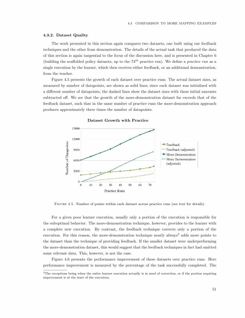
4.3 COMPARISON TO MORE MAPPING EXAMPLES
4.3.2. Dataset Quality
The work presented in this section again compares two datasets, one built using our feedbacktechniques and the other from demonstration. The details of the actual task that produced the dataof this section is again tangential to the focus of the discussion here, and is presented in Chapter 6(building the scaffolded policy datasets, up to the 74th practice run). We define a practice run as asingle execution by the learner, which then receives either feedback, or an additional demonstration,from the teacher.
Figure 4.5 presents the growth of each dataset over practice runs. The actual dataset sizes, asmeasured by number of datapoints, are shown as solid lines; since each dataset was initialized witha different number of datapoints, the dashed lines show the dataset sizes with these initial amountssubtracted off. We see that the growth of the more-demonstration dataset far exceeds that of thefeedback dataset, such that in the same number of practice runs the more-demonstration approachproduces approximately three times the number of datapoints.
Dataset Growth with Practice
Figure 4.5. Number of points within each dataset across practice runs (see text for details).
For a given poor learner execution, usually only a portion of the execution is responsible forthe suboptimal behavior. The more-demonstration technique, however, provides to the learner witha complete new execution. By contrast, the feedback technique corrects only a portion of theexecution. For this reason, the more-demonstration technique nearly always3 adds more points tothe dataset than the technique of providing feedback. If the smaller dataset were underperformingthe more-demonstration dataset, this would suggest that the feedback techniques in fact had omittedsome relevant data. This, however, is not the case.
Figure 4.6 presents the performance improvement of these datasets over practice runs. Hereperformance improvement is measured by the percentage of the task successfully completed. The
3The exceptions being when the entire learner execution actually is in need of correction, or if the portion requiring
improvement is at the start of the execution.
51

CHAPTER 4. ADVICE-OPERATORS
performance of both datasets is initially quite poor (0.58 ± 0.18% for more-demonstration, 5.99 ±0.24% for feedback, average of 10 executions). Across practice runs, the performance of the more-demonstration dataset does improve, marginally, to a 13.69 ± 0.02% success rate (average of 50executions). The performance of the feedback dataset is a marked improvement over this, improvingto a 63.32± 0.28% success rate4 (average of 50 executions).
Performance Improvement with Practice
Figure 4.6. Performance improvement of the more-demonstration and feedback policiesacross practice runs.
With these performance results, we may conclude that our feedback technique is omittingprimarily redundant data, that does not improve policy performance. Since the feedback dataset infact actually exceeds the performance of the more-demonstration dataset, we may further concludethat relevant data is being missed by demonstration, in spite of its larger dataset. Moreover, thisdata is being captured by teacher feedback.
4.4. Future Directions
The work presented in the following chapters of this thesis further validates advice-operators aseffective tools for correcting policies within continuous action-spaces. Many future directions for thedevelopment and application of advice-operators exist, a few of which are identified here. One is theapplication of action advice-operators to more complex spaces than 2-dimensional motion control,and another is the development of observation advice-operators. To conclude we consider feedbacktechniques that correct points within the demonstration dataset.
4.4.1. Application to More Complex Spaces
Advice-operators that influence translational and rotational speeds prescribe the limit of advice-operators explored in this thesis. This limit is motivated by two considerations. The first is our focus
4The feedback technique is able to achieve a 100% (approximately) success rate with more practice runs; see the
results in Section 6.2.2.3 for further details.
52

4.4 FUTURE DIRECTIONS
on motion control tasks for a Segway RMP robot, which is a wheeled differential drive robot withoutmanipulators or other motion control considerations requiring high-dimensional action-spaces. Thesecond is that this is a manageable action-space for the initial development and implementation ofthe advice-operator technique; namely, that translational and rotational speeds are straightforwardto isolate for the purposes of behavior correction and thus for advice-operator development.
Low-dimensional action-spaces do not, however, define the limit of advice-operators in gen-eral. The application of advice-operators to higher-dimensional action-spaces is not assumed to bestraightforward or obvious, and may require the development of additional translation techniques.For example, consider a manipulation task performed by a humanoid arm. An advice-operator thatinstructs the arm end effector to a different relative 3-D position in space, e.g. “more to the right”,might be simple for a feedback teacher to use, i.e. to identify as the fix for a particular executedbehavior. The workings of this advice-operator however, that translate “more to the right” intomodified joint angles and actuator speeds, are not simple, and advice-operator development there-fore is not straightforward. The introduction of an additional translation mechanism in this casecould be an inverse controller that translates 3-D end effector position into joint angles. The advice-operator then only needs to translate “more to the right” into a 3-D spatial position; a simpler taskthan the translation into joint angles and actuation speeds.
We identify the development of advice-operators for more complex action-spaces as a rich areafor future research. Until such research is performed, no concrete claims may be made about thefeasibility, or infeasibility, of advice-operators as tools for policy correction in high-dimensionalaction-spaces.
4.4.2. Observation-modifying Operators
The majority of the advice-operators developed for the work of this thesis are action-modifyingadvice-operators. Equally valid, however, are observation-modifying advice-operators.
The robot experiments of the following chapter (Ch. 5) will present one such observation-modifying example. The general idea of this technique will be to encode the target value for a goalinto the observation computation, and develop an operator that modifies the state-action mappingby resetting the target value of this goal to the executed value. In addition to behavior goals,target values for execution metrics could similarly be encoded into the observation computationand modified by an associated operator. This general idea - to encode a target value for someperformance or goal measure, and then modify it to match the executed value - is one option for thedevelopment of observation operators.
To develop operators that modify observation elements that are not a product of performancemetrics or goals, however, becomes more complicated. For example, to modify an observationthat computes the distance to a visually observed obstacle essentially amounts to hallucinatingobstacle positions, which could be dangerous. The development, implementation and analysis ofmore observation-modifying advice-operators is identified as an open ended and interesting directionfor future research.
53
CHAPTER 4. ADVICE-OPERATORS
4.4.3. Feedback that Corrects Dataset Points
Our corrective feedback technique modifies the value of learner-executed data, and thus correctspoints executed by the learner. Our negative binary credit feedback technique (Ch. 3) modifies theuse of the demonstration data by the policy, and thus credits points within the dataset. An interestingextension of these two techniques would be to define a feedback type that corrects points within thedataset.
Our advice-operator feedback technique corrects a policy by providing new examples of thecorrect behavior to the policy dataset. Poor policy performance can result from a variety of causes,including dataset sparsity, suboptimal demonstrations, and poor teacher-learner correspondence.These last two causes produce poor quality demonstration data. The more examples of good behaviorprovided through corrective feedback, the less influence this poor quality data will have on a policyprediction. The poor quality data will, however, always be present within the dataset, and thereforestill be considered to some extent by the regression techniques of the policy.
An alternate approach could correct the actual points within the dataset, instead of addingnew examples of good behavior. The advantage of such an approach would be to increase theinfluence of a correection and thus also the rate of policy improvement. A gradual overpowering ofthe suboptimal demonstration data with good examples would no longer be necessary, since the baddata would be corrected itself directly. How to determine which dataset points should be correctedwould depend on the regression technique. For example, with 1-NN regression, the single point thatprovided the regression prediction would be corrected. With more complex regression approaches,such as kernelized regression, points could be corrected in proportion to their contribution to theregression prediction, for example.
This approach is somewhat riskier than just adding new data to the set, since it assumes toknow the cause of the poor policy performance; namely, suboptimal demonstration data. As wasdiscussed in the previous chapter, there are many subtleties associated with crediting dataset pointsfor poor policy performance (Sec. 3.3.2.1). Taking care to correct only nearby datapoints wouldbe key to the soundness of this approach. Indeed, in our application of binary critique feedback,the extent to which demonstration datapoints are penalized is scaled inversely with the distancebetween that point and the query point for which the predication was made. The F3MRP frameworkalready computes a measure of dataset support for a given prediction; this measure could be used todetermine whether the dataset points contributing to the prediction should be corrected or not, forexample. Alternatively, this measure could be used to decide between two incorporation techniques;namely, to correct the dataset point if the prediction was well supported, and to add a new behaviorexample if the prediction was unsupported.
4.5. Summary
This chapter has introduced advice-operators as a mechanism for providing corrections tocontinuous-valued policies. Paired with the segment selection technique of our F3MRP frame-work, the approach becomes appropriate for correcting continuous-valued policies sampled at high
54
4.5 SUMMARY
frequency, such as those in motion control domains. In particular, the selection of a single execu-tion segment and single advice-operator enables the production of continuous-valued corrections formultiple execution datapoints.
We have presented our principled approach to the development of action advice-operators.Under this paradigm, a baseline set of operators are automatically defined from the available robotactions. A developer may then build new operators, by composing and sequencing existing operators,starting with the baseline set. The new datapoints produced from advice are additionally constrainedby parameters automatically set based on the robot dynamics, to firmly ground the synthesized dataon a real execution as well as the physical limits of the robot.
A comparison between datasets produced using exclusively demonstration versus our teacherfeedback techniques was additionally provided. The placement of data within the observation andaction spaces was shown to differ between the two approaches. Furthermore, the feedback techniqueproduced markedly smaller datasets paired with considerably improved performance. Note that inthe next chapter (Ch. 5) we will show policies derived from datasets built from teacher feedbackto exhibit similar or superior performance to those built from more teacher demonstration. InChapter 6 we will show not only superior performance, but the enablement of task completion.
Directions for future work with advice-operators were identified to include their applicationto more complex action spaces. Such an application would provide a concrete indication of thefeasibility, or infeasibility, of advice-operators as a tool for policy correction within high-dimensionalaction-spaces. The implementation of a full set of observation-modifying operators was another areaidentified for future research, along with operators that enact a broader impact by modifying thecontents of the dataset.
55


CHAPTER 5
Policy Improvement with Corrective Feedback
To correct a behavior executed by a robot learner is a very direct approach to policy refinement.Corrections encode more information than the binary credit feedback of the BC algorithm
(Ch. 3), by further indicating a preferred state-action mapping. Our contributed advice-operatorstechnique (Ch. 4) is an approach that simplifies providing policy corrections within continuousstate-action spaces. In this chapter we introduce Advice-Operator Policy Improvement (A-OPI) asan algorithm that employs advice-operators for policy improvement within a LfD framework (Argallet al., 2008). Two distinguishing characteristics of the A-OPI algorithm are data source and thecontinuity of the state-action space.
Data source is a key novel feature of the A-OPI approach. One common approach to policyimprovement within LfD is to add more teacher demonstration data in problem areas of the statespace and then re-derive the policy. Under A-OPI, more data is instead synthesized from learnerexecutions and teacher feedback, according to the advice-operator technique. In addition to notbeing restricted to the initial demonstration set contents, under this paradigm the learner moreoveris not limited to the abilities of the demonstrator.
Also key to A-OPI is its applicability to continuous state-action spaces. Providing correctionswithin continuous state-action spaces represents a significant challenge, since to indicate the correctstate or action involves a selection from an infinite set. This challenge is further complicated forpolicies sampled at high frequency, since to correct an overall executed behavior typically requirescorrecting multiple execution points and thus multiple selections from the infinite set. The A-OPI algorithm provides corrections through advice-operators and the segment selection techniqueof our F3MRP feedback framework. Under our algorithm, a single piece of advice there providescontinuous-valued corrections on multiple executions points. The A-OPI algorithm is thereforesuitable for continuous state-action policies sampled at high frequency, such as those present withinmotion control domains.
In this chapter we introduce A-OPI as an novel approach to policy improvement within LfD.A-OPI is validated on a Segway RMP robot performing a spatial positioning task. In this domain, A-OPI enables similar or superior performance when compared to a policy derived from more teacherdemonstrations. Furthermore, by concentrating new data exclusively to the areas visited by therobot and needing improvement, A-OPI produces noticeably smaller datasets.

CHAPTER 5. POLICY IMPROVEMENT WITH CORRECTIVE FEEDBACK
The following section introduces the A-OPI algorithm, providing the details of overall algorithmexecution. Section 5.2 presents a case study implementation of A-OPI, using simple advice-operatorsto correct a motion task. Section 5.3 presents an empirical implementation and evaluation of A-OPI,using a richer set of advice-operators to correct a more complex motion task. The conclusions ofthis work are provided in Section 5.4, along with the identification of directions for future research.
5.1. Algorithm: Advice-Operator Policy Improvement
The Advice-Operator Policy Improvement (A-OPI) algorithm is presented in this section. Tobegin, we briefly discuss providing corrections within the algorithm, followed by a presentation ofthe algorithm execution details.
5.1.1. Correcting Behavior with Advice-Operators
The purpose of advice within A-OPI is to correct the robot’s policy. Though this policy is un-known to the human advisor, it is represented by the observation-action mapping pairs of a studentexecution. To correct the policy, this approach therefore offers corrective information about theseexecuted observation-action pairings. The key insight to the A-OPI approach is that pairing a mod-ified observation (or action) with the executed action (or observation) now represents a correctedmapping. Assuming accurate policy derivation techniques, adding this datapoint to the demonstra-tion set and re-deriving the policy will thus correct the policy. Figure 5.1 presents a diagram ofdata synthesis from student executions and teacher advice (bottom, shaded box); for comparison,the standard source for LfD data from teacher executions is also shown (top).
Figure 5.1. Generating demonstration data under classical LfD (top) and A-OPI (bottom).
This work empirically explores advice-operators at two levels. The first looks at simple operatorsthat add static corrective amounts (Sec. 5.2). The second looks at more complex and flexibleoperators, that compute non-static corrective amounts according to functions that take as input thevalues of the executed observations or actions (Sec. 5.3).
Unlike BC, the incorporation of teacher feedback does not depend on the particulars of theregression technique, and any may be used. This implementation employs the Locally WeightedLearning regression technique described in Section 2.1.1.3. Here the observation-scaling parameter
58

5.1 ALGORITHM: ADVICE-OPERATOR POLICY IMPROVEMENT
Σ−1, within which the width of the averaging kernel is embedded, is tuned through Leave-One-Out-Cross-Validation (LOOCV). The implemented LOOCV minimizes the least squared error ofthe regression prediction, on the demonstration dataset D.
Teacher feedback under the A-OPI algorithm involves indicating an appropriate advice-operator,along with a segment of the execution over which to apply the operator. This feedback is used by thealgorithm to correct the learner execution. The corrected execution points are then treated as newdata, added to the demonstration set and considered during the next policy derivation. Figure 5.2presents a schematic of this approach, where dashed lines indicate repetitive flow and therefore ex-ecution cycles that are performed multiple times. In comparison to the schematic of the baselinefeedback algorithm (Fig. 2.4), note in particular the details of the dataset update.
Figure 5.2. Policy derivation and execution under the Advice-Operator Policy Improve-ment algorithm.
5.1.2. Algorithm Execution
Algorithm 3 presents pseudo-code for the A-OPI algorithm. This algorithm is founded on thebaseline feedback algorithm of Chapter 2. The distinguishing details of A-OPI lie in the type andapplication of teacher feedback (Alg. 1, lines 17-18).
The teacher demonstration phase produces an initial dataset D, and since this is identical tothe demonstration phase of the baseline feedback algorithm (Alg. 1, lines 1-8), for brevity the details
59

CHAPTER 5. POLICY IMPROVEMENT WITH CORRECTIVE FEEDBACK
of teacher execution are omitted here. The learner execution portion of the practice phase (Alg. 3,lines 5-9) also proceeds exactly as in the baseline algorithm, recording the policy predictions androbot positions respectively into the execution traces d and tr.
Algorithm 3 Advice-Operator Policy Improvement
1: Given D2: initialize π ← policyDerivation(D)3: while practicing do4: initialize d← {}, tr ← {}5: repeat6: predict at ← π (zt)7: execute at
8: record d ← d ∪ (zt,at) , tr ← tr ∪ (xt, yt, θt)9: until done
10: advise { op,Φ } ← teacherFeedback( tr )11: for all ϕ ∈ Φ, (zϕ,aϕ) ∈ d do12: if op is observation-modifying then13: modify (zϕ,aϕ) ← (op (zϕ) ,aϕ)14: else {op is action-modifying}15: modify (zϕ,aϕ) ← (zϕ, op (aϕ))16: end if17: end for18: update D ← D ∪ dΦ
19: rederive π ← policyDerivation(D)20: end while21: return π
During the teacher feedback portion of the practice phase, the teacher first indicates a segmentΦ, of the learner execution trajectory requiring improvement. The teacher feedback is an advice-operator op ≡ z (Sec. 2.4.2), selected from a finite list, to correct the execution within this segment(line 10).
The teacher feedback is then applied across all points recorded in d and within the indicatedsubset Φ (lines 11-17); this code segment corresponds to the single applyFeedback line of Algo-rithm 1. For each point ϕ ∈ Φ, (zϕ,aϕ) ∈ d, the algorithm modifies either its observation (line 13)or action (line 15), depending on the type of the indicated advice-operator. The modified datapointsare added to the demonstration set D (line 18).
These details of advice-operator application are the real key to correction incorporation. Tothen incorporate the teacher feedback into the learner policy simply consists of rederiving the policyfrom the dataset D, now containing new advice-modified datapoints (line 19).
5.2. Case Study Implementation
This section presents a case-study implementation of the A-OPI algorithm on a real robotsystem. The task is executed by a Segway RMP robot, which is a dynamically balancing differentialdrive platform produced by Segway LLC (Nguyen et al., 2004). Initial results are promising, showing
60

5.2 CASE STUDY IMPLEMENTATION
improved performance with corrective advice and superior performance to providing further teacherdemonstrations alone.
5.2.1. Experimental Setup
As a first study of the effectiveness of using advice-operators, algorithm A-OPI is applied tothe task of following a spatial trajectory with a Segway RMP robot (Fig. 5.3). First presented arethe task and advice-operators for this domain, followed by empirical results.
Figure 5.3. Segway RMP robot performing the spatial trajectory following task (approx-imate ground path drawn in yellow).
5.2.1.1. Spatial Trajectory Following Task and Domain. Within this case-study, thelearner is tasked with following a sinusoidal spatial trajectory. The robot senses its global positionand heading within the world through wheel encoders sampled at 30Hz. The observations computedby the robot are 3-dimensional: x-position, y-position, and robot heading (x, y, θ). The actionspredicted are 2-dimensional: translational speed and rotational speed (ν, ω).
Teacher demonstrations of the task are performed via joystick teleoperation of the robot. Tochallenge the robustness of A-OPI, the demonstration set was minimal and contained only oneteacher execution (330 datapoints). A total of three policies are developed for this task:
Baseline Policy: Derived from the initial demonstration set.
Feedback Policy: Provided with policy corrections, via advice-operators.
More Demonstration Policy: Provided with more teacher demonstrations.
The learner begins practice with the Baseline Policy. The incorporation of teacher feedback on thelearner executions updates this policy. This execution-feedback-update cycle continues to the satisfac-tion of the teacher, resulting in the Feedback Policy. For comparison, a policy that instead receivesmore teacher demonstrations is also developed, referred to as the More Demonstration Policy. Thispolicy is provided with additional demonstration traces, so that the size of its dataset approximatelymatches that of the Feedback Policy dataset (two additional demonstrations provided).
The motion control advice-operators for this study were developed by hand and have a basicformulation (Table 5.1). Each operator adjusts the value of a single action dimension, by a staticamount.
61

CHAPTER 5. POLICY IMPROVEMENT WITH CORRECTIVE FEEDBACK
Operator Parameter0 Modify Speed, static, small (rot) [ cw ccw ]1 Modify Speed, static, large (rot) [ cw ccw ]2 Modify Speed, static, small (tr) [ dec inc ]3 Modify Speed, static, large (tr) [ dec inc ]
Table 5.1. Advice-operators for the spatial trajectory following task.
[Key: (rot/tr)=(rot/transl)ational, (c)cw=(counter)clockwise], (dec/inc)=(de/in)crease]
5.2.1.2. Evaluation. For this task, executions are evaluated for efficiency and precision.Efficiency is defined by execution time. Precision is defined by how closely the target sinusoidalpath is followed, computed as the mean-squared Euclidean distance to this path.
The intent of this case-study is to explore behavior changes that might be enacted throughadvice-operators. We focus in particular on (i) improvement beyond the demonstrator’s abilitiesand (ii) the synthesis of new behavior characteristics.
One behavior change seen in the empirical BC results was the potential for the learner toimprove beyond the performance of the demonstration teacher. To investigate this, the performanceof the Feedback Policy will be compared to the performance of the teleoperation demonstration thatpopulated the initial dataset.
Another theoretical behavior change to explore is whether the presence of synthesized dataalso enables the synthesis of new behavior characteristics. Improvements under the BC algorithmwere restricted to the data demonstrated by the teacher; critiquing just enabled the consideration ofsome points more strongly than others when making predictions. With A-OPI, however, new statesand actions are made available to the policy, through the advice-operator data synthesis technique.To explore the ability of A-OPI to generate new behavior characteristics, the initial demonstrationset provided to the learner is intentionally deficient in some behavior characteristics desired in thefinal policy. The goal is to generate these characteristics through the use of advice-operators. Moreconcretely, the demonstration set contains point turns and, for smoothness considerations, it isdesired that these be absent from executions with the final policy.
5.2.2. Results
Policy performance was found to improve with corrective feedback. The robot learner was ableto improve its performance beyond the capabilities in its demonstration set, with faster executiontimes and more precisely executed positioning. Furthermore, the advisor was able to guide thelearner to a policy with features that were not attainable within the original demonstration dataset;namely, the absence of point turns.
5.2.2.1. Improvement Beyond the Demonstration Set. Precision results are presentedwithin Figure 5.4, as the average positional error between the execution path and the target sinusoid.Each bar represents the mean of 5 executions (1-standard deviation error bars). For comparison,the performance of the single teacher demonstration execution that populated the initial dataset isalso shown (Teacher Demo, no error bars).
62

5.2 CASE STUDY IMPLEMENTATION
Advising improved execution precision (Feedback). This improvement was seen over the initialpolicy (Baseline), as well as over the teleoperation execution provided as a demonstration (TeacherDemo). This latter result indicates that advice-operators are indeed able to produce performanceimprovements beyond capabilities present in the demonstration set.
More teleoperation demonstrations also improved policy performance, with the policy de-rived from this set (More Demonstration) outperforming the initial policy (Baseline). This more-demonstration policy however was not able to perform as well as the A-OPI policy (Feedback).Moreover, unlike the feedback policy, providing more teleoperations also was not able to improveupon the performance of the teacher demonstration recorded in the initial demonstration dataset.
Positional Execution Error
(A) (B) (C) (D)
Figure 5.4. Execution trace mean position error compared to target sinusoidal trace.
Advising further resulted in a reduction in execution time, presented in Table 5.2. This isattributed to smoother executions without point turns (discussed in the following section), as wellas to faster translational speeds, enabled through the use of the operators that increase translationalspeed. Again, the advised policy (Feedback) outperforms those derived from only teleoperation(Baseline, More Demo), as well as the teacher execution within the demonstration set (TeacherDemonstration).
Teacher Demonstration Baseline Feedback More Demonstration10.89 11.35 7.62 10.8
Table 5.2. Average execution time (in seconds).
5.2.2.2. New Behavior Characteristics. Figure 5.5 shows examples of position tracesduring execution. For each, the target sinusoidal path (thin red line) and the execution trace (thickblue line) are shown. The letter labels attached to these executions indicate: (A) teacher demonstra-tion execution, (B) initial policy execution (Baseline Policy), (C) policy execution after feedback
63

CHAPTER 5. POLICY IMPROVEMENT WITH CORRECTIVE FEEDBACK
(Feedback Policy), and (D) policy execution with more demonstration data (More DemonstrationPolicy). These labels correlate to the bars left to right in Figure 5.4.
(A) (B)
(C) (D)
Figure 5.5. Example execution position traces for the spatial trajectory following task.
Plot (A) shows the execution trace of the single teacher demonstration used to populate thedemonstration set. Note that this execution does not perfectly follow the target sinusoidal path,and that point turns were executed at the two points of greatest curvature (indicated by the tracedoubling back on itself, a side-effect of the Segway platform’s dynamic balancing).
A learner execution using the Baseline Policy derived from this demonstration set is shown inplot (B). This execution follows the target sinusoid more poorly than the demonstration trace, due todataset sparsity, and similarly executes point turns. This learner execution was then advised, and thepath re-executed using the modified policy. This process was repeated in total 12 times. Executionwith the final Feedback Policy is shown in plot (C). This execution follows the target sinusoidbetter than the Baseline Policy execution and better than the teacher demonstration execution.Furthermore, this execution does not contain point turns.
Using the policy derived from more teleoperation data, shown in plot D, the learner is betterable to follow the sinusoid than with the Baseline Policy; compare, for example, to the executionin plot (A). However, the learner is not able to smooth out its execution, and neither is it able toeliminate point turns.
5.2.3. Discussion
In this section we first present our conclusions from this case study. We then discuss a relation-ship between the demonstration approach taken in this case study and our approach for scaffolding
64
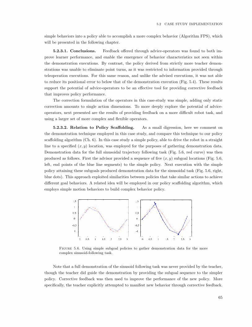
5.2 CASE STUDY IMPLEMENTATION
simple behaviors into a policy able to accomplish a more complex behavior (Algorithm FPS), whichwill be presented in the following chapter.
5.2.3.1. Conclusions. Feedback offered through advice-operators was found to both im-prove learner performance, and enable the emergence of behavior characteristics not seen withinthe demonstration executions. By contrast, the policy derived from strictly more teacher demon-strations was unable to eliminate point turns, as it was restricted to information provided throughteleoperation executions. For this same reason, and unlike the advised executions, it was not ableto reduce its positional error to below that of the demonstration execution (Fig. 5.4). These resultssupport the potential of advice-operators to be an effective tool for providing corrective feedbackthat improves policy performance.
The correction formulation of the operators in this case-study was simple, adding only staticcorrection amounts to single action dimensions. To more deeply explore the potential of advice-operators, next presented are the results of providing feedback on a more difficult robot task, andusing a larger set of more complex and flexible operators.
5.2.3.2. Relation to Policy Scaffolding. As a small digression, here we comment onthe demonstration technique employed in this case study, and compare this technique to our policyscaffolding algorithm (Ch. 6). In this case study a simple policy, able to drive the robot in a straightline to a specified (x, y) location, was employed for the purposes of gathering demonstration data.Demonstration data for the full sinusoidal trajectory following task (Fig. 5.6, red curve) was thenproduced as follows. First the advisor provided a sequence of five (x, y) subgoal locations (Fig. 5.6,left, end points of the blue line segments) to the simple policy. Next execution with the simplepolicy attaining these subgoals produced demonstration data for the sinusoidal task (Fig. 5.6, right,blue dots). This approach exploited similarities between policies that take similar actions to achievedifferent goal behaviors. A related idea will be employed in our policy scaffolding algorithm, whichemploys simple motion behaviors to build complex behavior policy.
Figure 5.6. Using simple subgoal policies to gather demonstration data for the morecomplex sinusoid-following task.
Note that a full demonstration of the sinusoid following task was never provided by the teacher,though the teacher did guide the demonstration by providing the subgoal sequence to the simplerpolicy. Corrective feedback was then used to improve the performance of the new policy. Morespecifically, the teacher explicitly attempted to manifest new behavior through corrective feedback.
65
CHAPTER 5. POLICY IMPROVEMENT WITH CORRECTIVE FEEDBACK
The target new behavior was smooth sinusoidal trajectory following with an absence of pauses andpoint turns. The pauses and points turns were a consequence of sequential subgoal execution withthe simpler policy, coupled with the dynamic balancing of this robot platform. The new behavior,without pauses and point turns, was achieved (Fig. 5.5, C). In the case of this approach, feedbackwas used to shape a new policy behavior, by removing residual behavior characteristics seen duringdemonstration executions. Moreover, feedback enabled the development of a more complex policyfrom a simpler existing policy. The same principles will be true for our policy scaffolding algorithm.
5.3. Empirical Robot Implementation
This section presents results from the application of A-OPI to a more difficult motion task,again with a Segway RMP robot, and using a set of more complex operators. Policy modificationsdue to A-OPI are shown to improve policy performance, both in execution success and accuracy.Furthermore, performance is found to be similar or superior to the typical approach of providingmore teacher demonstrations (Argall et al., 2008).
5.3.1. Experimental Setup
Here the experimental details are presented, beginning with the task and domain, and followedby advice-operator and policy developments.
5.3.1.1. Robot Spatial Positioning Task and Domain. Empirical validation of theA-OPI algorithm is performed through spatial positioning with a Segway RMP robot. The spatialpositioning task consists of attaining a 2-D planar target position (xg, yg), with a target heading θg.
The Segway RMP platform accepts wheel speed commands, but does not allow access to itsbalancing control mechanisms. We therefore treat Segway RMP control as a black box, since we donot know the specific gains or system parameter values. The inverted pendulum dynamics of therobot present an additional element of uncertainty for low level motion control. Furthermore, forthis task smoothly coupled rotational and translational speeds are preferred, in contrast to turningon spot to θg after attaining (xg, yg). To mathematically define for this specific robot platform thedesired motion trajectories for this task is thus non-trivial, encouraging the use of alternate controlapproaches such as A-OPI. That the task is straightforward for a human to evaluate and correctfurther supports A-OPI as a candidate approach. While the task was chosen for its suitabilityto validate A-OPI, to our knowledge this work also constitutes the first implementation of such amotion task on a real Segway RMP platform.
The robot observes its global position and heading through wheel encoders sampled at 30Hz.Let the current robot position and heading within the world be represented as (xr, yr, θr), andthe vector pointing from the robot position to the goal position be (xv, yv) = (xg − xr, yg − yr).The observations computed for this task are 3-dimensional: squared Euclidean distance to the goal(x2v + y2
v), the angle between the vector (xv, yv) and robot heading θr, and the difference betweenthe current and target robot headings (θg − θr). The actions are 2-dimensional: translational speedand rotational speed (ν, ω).
66

5.3 EMPIRICAL ROBOT IMPLEMENTATION
5.3.1.2. Motion Control Advice-Operators. Presented in Table 5.3 are the operatorsdeveloped for this task. These operators adjust observation inputs (as in operator 0), single actiondimensions by non-static amounts (as in operators 1-6) or multiple action dimensions by non-staticamounts (as in operators 7,8). The amount of the non-static adjustments are determined as afunction of the executed observation/action values. Note that these operators were developed byhand, and not with our principled development approach presented in the previous chapter (Sec. 4.2).The operators are general to other motion tasks with this robot platform, and could be applied withinother motion control domains.
Operator Parameter0 Reset goal, recompute observation -1 No rotational speed -2 Add rotational speed [ cw ccw ]3 Smooth rotational speed [ dec inc ]4 No translational speed -5 Smooth translational speed [ dec inc ]6 Translational acceleration [ dec inc ]7 Turn tightness [ less more ]8 Stop all motion -
Table 5.3. Advice-operators for the spatial positioning task.
[Key: (c)cw=(counter)clockwise, (dec/inc)=(de/in)crease]
5.3.1.3. Policy Development. The set D is seeded with demonstrations recorded as theteacher teleoperates the robot learner (5 goal locations, with some repeat demonstrations for a totalof 9 demonstrations, producing 900 data points). An initial policy is derived from this dataset.
Policy improvement proceeds as follows. A goal is selected (without replacement) from a prac-tice set consisting of (x, y, θ) goals drawn uniformly within the bounds of the demonstration datasetx ∼ U (−0.33, 4.5m) , y ∼ U (−4.0, 0.17m) , θ ∼ U (−3.1, 1.1rad). The robot executes its currentpolicy to attain this goal. The advisor observes this execution. If the execution is considered poor,the advisor offers policy improvement information. The policy is re-derived. Drawing a new goalthen initiates another practice run, defined as a single execute-feedback-update cycle.
Three policies are developed using distinct techniques, differing in what is offered as policyimprovement information. A total of four policies are therefore developed within this domain:
Baseline Policy: Derived from the initial demonstration set.
Feedback Policy: Provided with policy corrections, via advice-operators.
Feedback Hybrid Policy: Initially provided with more teacher demonstrations; later pro-vided with policy corrections via advice-operators.
More Demonstration Policy: Provided with more teacher demonstrations.
67

CHAPTER 5. POLICY IMPROVEMENT WITH CORRECTIVE FEEDBACK
The final three are referred to collectively as the improvement policies. Note that in the case of theMore Demonstration Policy, a practice run consists of a single execute-demonstrate-update cycle.
Policy performance is evaluated on a test set, consisting of 25 (x, y, θ) goals, randomly drawnfrom a uniform distribution within the bounds of the demonstration dataset. The test set is in-dependent, and no executions associated with it receive policy improvement information. Policiesare evaluated for accuracy and success. Here accuracy is defined as Euclidean distance between thefinal robot and goal positions ex,y = ‖(xg − xr, yg − yr)‖, and the final robot and goal headingseθ = |θg − θr|. Success is defined generously as ex,y < 1.0 m and eθ <
π2 rad.
5.3.2. Results
Policy performance was found to improve with A-OPI feedback, in both execution success andaccuracy. When compared to the approach of providing more teleoperation data, final improvementamounts were found to be similar or superior. Furthermore, this performance was achieved with asimilar number of practice executions, but a significantly smaller final dataset.
For each policy improvement approach, the policy improvement phase was halted once per-formance on the test set no longer improved. The final Feedback, Feedback Hybrid and MoreDemonstration Policies respective contained data from 60, 59 and 51 practice runs, in additional tothe 9 initial demonstrations of the Baseline Policy.
5.3.2.1. Success and Accuracy Improvement. Table 5.4 presents the percent executionsuccess of each policy on the independent test set. When compared to the Baseline Policy, allpolicy improvement approaches display increased success. Both of the feedback policies additionallyachieve higher success than the More Demonstration Policy.
Baseline Feedback Feedback Hybrid More Demonstration32 88 92 80
Table 5.4. Execution percent success, test set.
Figure 5.7 plots the average position and heading error on the test set goals, for each policy.For positional error, all improvement policies display similar performance, which is a dramaticimprovement over the Baseline Policy. For heading, the Feedback Policy reduces more error thanthe Feedback Hybrid Policy, with both showing marked improvements over the Baseline Policy. Bycontrast, the More Demonstration Policy displays no overall improvement in heading error. Thatheading error proved in general more difficult to improve than positional error is consistent with ourprior experience with this robot platform, which is highly sensitivity to rotational dead reckoningerror accumulation.
The iterative nature of the A-OPI policy development approach (Section 5.3.1.3) results inintermediate policies being produced. A sampling of these policies were also evaluated on the test set,to mark improvement progress for each policy improvement technique. Figure 5.8 shows the averageposition and heading error, on the test set goals, for these intermediate policies. Superior heading
68
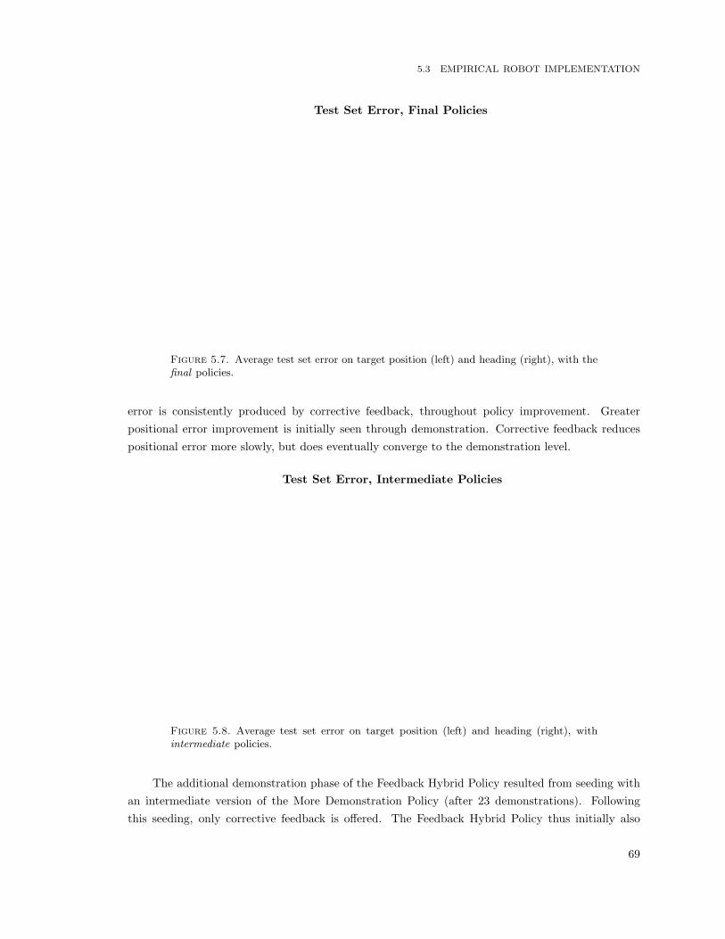
5.3 EMPIRICAL ROBOT IMPLEMENTATION
Test Set Error, Final Policies
Figure 5.7. Average test set error on target position (left) and heading (right), with thefinal policies.
error is consistently produced by corrective feedback, throughout policy improvement. Greaterpositional error improvement is initially seen through demonstration. Corrective feedback reducespositional error more slowly, but does eventually converge to the demonstration level.
Test Set Error, Intermediate Policies
Figure 5.8. Average test set error on target position (left) and heading (right), withintermediate policies.
The additional demonstration phase of the Feedback Hybrid Policy resulted from seeding withan intermediate version of the More Demonstration Policy (after 23 demonstrations). Followingthis seeding, only corrective feedback is offered. The Feedback Hybrid Policy thus initially also
69
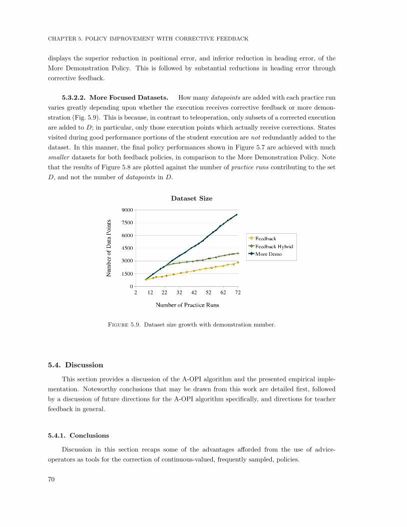
CHAPTER 5. POLICY IMPROVEMENT WITH CORRECTIVE FEEDBACK
displays the superior reduction in positional error, and inferior reduction in heading error, of theMore Demonstration Policy. This is followed by substantial reductions in heading error throughcorrective feedback.
5.3.2.2. More Focused Datasets. How many datapoints are added with each practice runvaries greatly depending upon whether the execution receives corrective feedback or more demon-stration (Fig. 5.9). This is because, in contrast to teleoperation, only subsets of a corrected executionare added to D; in particular, only those execution points which actually receive corrections. Statesvisited during good performance portions of the student execution are not redundantly added to thedataset. In this manner, the final policy performances shown in Figure 5.7 are achieved with muchsmaller datasets for both feedback policies, in comparison to the More Demonstration Policy. Notethat the results of Figure 5.8 are plotted against the number of practice runs contributing to the setD, and not the number of datapoints in D.
Dataset Size
Figure 5.9. Dataset size growth with demonstration number.
5.4. Discussion
This section provides a discussion of the A-OPI algorithm and the presented empirical imple-mentation. Noteworthy conclusions that may be drawn from this work are detailed first, followedby a discussion of future directions for the A-OPI algorithm specifically, and directions for teacherfeedback in general.
5.4.1. Conclusions
Discussion in this section recaps some of the advantages afforded from the use of advice-operators as tools for the correction of continuous-valued, frequently sampled, policies.
70

5.4 DISCUSSION
5.4.1.1. Advice-Operator Selection and Application. These empirical results confirmthat a human teacher was able to effectively advise within continuous action spaces using the A-OPIalgorithm. This occurred without requiring that the teacher provide the actual continuous-values forthe corrections. Additionally, the teacher was able to select operators without requiring value-baseddetails of the execution (e.g. speed). Both of these aspects result from the fact that the robot, andnot the human, applies the advice-operator.
One goal when developing the motion control operators of this domain was to exploit therespective strengths of a robot learner and human teacher. Humans in general are good at providingqualitative evaluations of performance quickly and accurately (for example, “drive faster”), but areless adept at determining exact quantitative measures (for example, “drive exactly 1.6ms ”). Bycontrast, the robot has access to its internal state including current driving speeds, and is able toreason quickly and accurately about quantity.
5.4.1.2. An Observation Advice-Operator. The operators developed for this task in-cluded one example of an observation-modifying advice-operator: the operator “Reset goal, recom-pute observation”. The observations computed for the spatial positioning task encoded the targetfinal position and heading (xg, yg, θg). This operator functioned by resetting the target to be theactual final position and heading (xf , yf , θf ) attained during an execution. The operator then re-computed all of the observations along the execution path as though this final position/heading(xf , yf , θf ) had been the target position/heading. This operator was applied to executions thatexhibited a path that performed well according to the measures of speed and path smoothness, butpoorly according to the measure of accurately attaining the target position/heading. The intent ofthis operator was to remember such executions as good examples of attaining the position/heading(xf , yf , θf ).
As mentioned in the previous chapter (Sec. 4.4.2), the general idea of this technique is to encodethe target value for a goal - here the target (x, y, θ) position - into the observation computation,and to develop an operator that modifies the state-action mapping by resetting the target valueto the executed value. The single operator presented here constitutes only a small exploration ofobservation-modifying advice-operators, and a more complete investigation is identified as a richarea for future research.
5.4.1.3. Advising is a Reasonable Task. Teacher feedback under A-OPI consists ofselecting segments of an execution requiring improvement and indicating an advice-operator to applyover this segment. In this manner, the selection of a single execution segment and single advice-operator from a finite list enables the continuous-valued correction of multiple execution points.This quality makes A-OPI suitable for domains with continuous actions sampled at high frequency,such as low-level motion control domains. Without such a mechanism, to provide continuous-valuedcorrections for a large number of executions points would be highly taxing on a human teacher.With A-OPI, this becomes a reasonable task for the feedback teacher.
Our feedback teacher was able to provide advice quickly, for a variety of reasons. One reasonwas the ability to advise multiple execution points at once, through the F3MRP segment selectiontechnique. Another reason was that the A-OPI algorithm is robust to fuzzy selections of execution
71
CHAPTER 5. POLICY IMPROVEMENT WITH CORRECTIVE FEEDBACK
points, and the cause of this is twofold. First, since our employed regression techniques treat eachdatapoint independently, a point added to the dataset does not depend on whether nearby pointsfrom the execution were also added. Second, since the policy is sampled rapidly and exists withina continuous state-action space, physical constraints on the robot and world mandate that adjacentexecution points are similar in both observation and action values; our robot has the ability neitherto teleport nor to infinitely accelerate. This similarity makes it unlikely that a correction would beappropriate for one point but inappropriate for its neighbor.
Chapter 3 discussed the benefit of having a human teacher provide the critiquing feedback(Sec. 3.3.1.2). While the automation of simple overall evaluations of an execution was noted to befeasible, the ability of a human to address the issue of credit assignment was highlighted as a strength.When providing corrective advice, the human teacher again addresses the issue of which portionsof an execution receive feedback. Here, however, the evaluation tied to the feedback additionallyis not simple or straightforward. That is, to provide a correction is more complex than providingan overall binary evaluation of success. Not only are more complex evaluation measures employed,for example if a turn was “tight” enough, but based on these evaluations a correction must beselected. Advice-operators simplify this process, by offering a finite list for this selection. Even withthis simplification, however, it is unlikely that some form of automated feedback would be able toprovide a correction, again highlighting the strength of a human feedback provider.
5.4.2. Future Directions
This section identifies potential areas for future research with the A-OPI algorithm. The firstoption considered is to interleave corrective feedback and demonstration. We then consider alternateformulations for corrective feedback.
5.4.2.1. Policy Improvement from Advice and Demonstration. Two improvementapproaches, advising and more teleoperation, were considered by the hybrid policy. More specifically,the hybrid policy was seeded with an intermediate version of the More Demonstration Policy andthen provided with corrective feedback, in an attempt to exploit the strengths of each technique. Thisapproach was motivated from noting that (i) more demonstration quickly reduced initial positionalerror but struggled to reduce heading error, and (ii) corrections gradually reduced both types of erroroverall. The supposed reason for this difference is that demonstration is more effective at reachingpreviously undemonstrated areas of the state space; by contrast, corrections can only be offered onstates already visited, and therefore already reachable with the current policy. Correspondingly,advice-operators are more effective at correcting visited states; by contrast, it is difficult for theteacher to revisit real world states through teleoperation, especially when those states lie in themiddle of a motion trajectory.
These observations underline the benefit of providing both corrections and more demonstration.Advice-operators are most effective when correcting an already adequate policy; using advice to iter-atively modify action selection in order to creep towards a distant desirable part of the state-space isinefficient and not recommended. By contrast, demonstration is most effective for general state-spacepopulation; using teleoperation in an attempt to exactly revisit states and demonstrate alternate
72
5.5 SUMMARY
behaviors is similarly inefficient and not recommended. The approaches, in short, compliment eachother.
In this implementation of the hybrid policy, more demonstration and corrective feedback hap-pened in distinct phases. While some demonstration does need to occur first, to provide a baselinepolicy for advising to build upon, demonstration does not need to occur only first. One directionfor future work could interleave providing corrections and more demonstration. Alternately, a suffi-ciently populated demonstration set could be provided at the start. This is fundamentally different,however, to providing more demonstration in response to student executions. A sufficiently pop-ulated dataset requires prior knowledge of all states the student will visit; generally impossible incontinuous-state real worlds.
5.4.2.2. Other Options for Corrective Advice. Advice-operators offer a formulationfor corrective advice within continuous state-action domains. The key contribution of this techniqueis the functional formulation of advice-operators, where mathematical computations are performedon execution data points. The functional formulation makes providing continuous-valued correctionsreasonable, and is less appropriate for providing discrete-valued corrections. To provide a fractionalcorrection to a high-level, discrete action, behavior policy is less immediate; for example, to increase apick-up-box action by 20% does not make sense. This does not mean, however, that advice-operatorsare not applicable within discrete action domains; it is just not appropriate for their formulationto fragment actions. One appropriate formulation, for example, could adjust the number times arepetitive discrete action is executed, such as the number of discrete steps taken by a humanoidrobot. Advice-operators therefore may be appropriate for some discrete-action domains, but notnecessarily for all.
Many other formulations for corrective feedback are also possible, and we present some exampleshere. One already noted is the selection of a correct action from a discrete set, within discrete-actiondomains. A higher-level example is a behavior that operates by selecting between multiple policies,as will be the case with our policy scaffolding algorithm presented in the next chapter. A correctionwithin this scenario could indicate the appropriate policy to select (note that this corrections is aconjecture only, and is not included within our policy scaffolding algorithm). Another hypotheticalpolicy formulation could involve selection between multiple weightings on the observation space, tovary the importance given to different observation features within distinct areas of the state space.Corrective feedback in this domain could correct the selection of observation weight.
5.5. Summary
This chapter has introduced Advice-Operator Policy Improvement (A-OPI) as an algorithmthat improves the performance of a policy learned through demonstration via the use of correctiveteacher feedback. Here teacher feedback results in new, synthesized, demonstration data, that doesnot depend on teacher demonstrations nor revisiting past execution states.
Empirical validation of A-OPI was performed on a Segway RMP robot performing planar mo-tion tasks. The first implementation was a case study that used a simple set of advice-operators tocorrect a spatial trajectory following task. Empirical results showed improvements in precision and
73

CHAPTER 5. POLICY IMPROVEMENT WITH CORRECTIVE FEEDBACK
efficiency, and both beyond the abilities of demonstrator. Corrective advice was also found to enablethe emergence of novel behavior characteristics, absent from the demonstration set. The secondimplementation used a complex set of advice-operators to correct a more difficult spatial positioningtask. Empirical results showed performance improvement, measured by success and accuracy. Fur-thermore, the feedback policies displayed similar or superior performance when compared to a policydeveloped from exclusively more teleoperation demonstrations. The A-OPI approach also producednoticeably smaller datasets, without a sacrifice in policy performance, suggesting that the datasetswere more focused and contained less redundant data.
Key features of the A-OPI approach facilitate the ability to provide corrections within low-level motion control domains. In particular, the segment selection technique allows multiple actionsto be corrected by a single piece of advice. The advice-operator mechanism translates high-leveladvice into continuous-valued corrections. Selection of an operator is reasonable for a human toperform, since the set of advice-operators is discrete; by contrast, selection from an infinite set ofcontinuous-valued corrections would not be reasonable.
Future directions for the A-OPI algorithm were identified to include interleaving the two policyimprovement techniques of corrective advice and more teleoperation demonstrations. The formula-tion of corrective advice within other domains was also discussed.
74

CHAPTER 6
Policy Scaffolding with Feedback
Given the challenge of developing robust control policies, the ability to reuse and combine policiesdesigned to address related tasks is a practical feature for any policy learning system. While LfD
has seen success on a variety of robotics applications, as tasks become more complex, demonstrationcan become more difficult. One practical extension of the LfD approach thus is to incorporate simplerbehaviors learned from demonstration into larger tasks, especially if such tasks are too complex todemonstrate in full. We introduce Feedback for Policy Scaffolding (FPS) as an algorithm that buildsa complex policy from component behaviors learned from demonstration.
One crucial issue when building a policy from primitives is how to effectively incorporate theexisting behaviors into the new policy. Whether the behaviors are to be composed or sequenced,behaviors must be linked and how this linking occurs is a key design decision. The FPS algorithmtakes the approach of aiding this process with human feedback. The feedback types considered bythis algorithm are binary flags of good performance and corrective advice, provided through theadvice-operator framework (Ch. 4). Advice under this formulation does not require revisiting statesto provide feedback, which is particularly attractive for complex tasks that may be inconvenient orinfeasible to demonstrate completely.
This chapter contributes an algorithm that extends the A-OPI algorithm by selecting betweenmultiple policies and incorporating an additional feedback phase. In phase one of the FPS algorithm,multiple policies are developed from demonstrated motion primitives, using a slightly modified ver-sion of the A-OPI algorithm (Ch. 5). During phase two, a single complex policy is derived from theseprimitives, and executions with the complex policy on a novel task are evaluated. By providing cor-rections on this execution, the FPS algorithm develops a policy able to execute this more complex,undemonstrated task. This development is achieved without ever requiring a full demonstration ofthe novel task.
We validate FPS within a simulated motion control domain, where a robot learns to drive ona racetrack. A policy built from demonstrated motion primitives and human feedback is developedand able to successfully execute a more complex, undemonstrated task. Advice is shown to improvepolicy performance within both feedback phases: when offered in response to individual motionprimitive executions, as well as executions with the complex task policy. Finally, comparisons to an

CHAPTER 6. POLICY SCAFFOLDING WITH FEEDBACK
exclusively demonstration-based approach show the FPS algorithm to be more concise and effectivein developing a policy able to execute the complex task.
The following section introduces the FPS algorithm, providing details of behavior buildingthrough teacher feedback and algorithm execution. Section 6.2 presents an empirical implementationof FPS, including descriptions of the task and domain. Experimental results, from both feedbackphases, are also provided. The conclusions of this work are presented in Section 6.3, along withdirections for future research.
6.1. Algorithm: Feedback for Policy Scaffolding
This section presents the Feedback for Policy Scaffolding algorithm. The section begins bymotiving why a more complex policy is built from demonstration and teacher feedback. This isfollowed with a discussion of the algorithm execution details.
6.1.1. Building Behavior with Teacher Feedback
We begin with a discussion of some reasons why one might use teacher feedback to build apolicy that produces a more complex behavior, rather than demonstrating that behavior outright.One consideration is that as behaviors become more complex, demonstrating the behavior in full canbecome more difficult. In this case, the teacher may be able to demonstrate behavior primitives forthe task but not the task in full, or be able to provide higher quality demonstrations for primitivesthan for the full task. Under our algorithm, feedback may be used to improve, possibly even toenable, the policy at transition points that link demonstrated behavior primitives. In doing so, itenables expression of the full task behavior, without requiring its full demonstration.
A second consideration is that reaching all states encountered during task execution can becomeincreasingly difficult as tasks become more complex. States may be infeasible, inconvenient orundesirable to reach for a variety of reasons that only compound as task complexity increases.A drawback to demonstration is the need to visit such states in order to provide task executioninformation in that area. One of the notable benefits of providing feedback under the F3MRPframework is that states do not need to be revisited to provide execution feedback.
A final consideration is that the demonstrated motion primitives may provide a base for multiplecomplex behaviors. Through the reuse of these primitives, the effort required to develop policies forthe complex behaviors reduces.
6.1.2. Feedback for Policy Scaffolding Algorithm Execution
Algorithms 4 and 5 present pseudo-code for the FPS algorithm. This algorithm is founded onthe baseline feedback algorithm of Chapter 2. The distinguishing details of FPS lie in the typesand applications of teacher feedback (Alg. 1, lines 17-18) and the development of multiple primitivepolicies. The FPS algorithm furthermore includes of a second phase of learner practice during whichthe primitive policies are scaffolded together.
Execution occurs in two phases. Given a set Ξ of n primitive behaviors, the first phase developsa policy πξj for each primitive behavior ξj ∈ Ξ, j = 1 . . . n, producing a set of policies Π (Alg. 4).
76
6.1 ALGORITHM: FEEDBACK FOR POLICY SCAFFOLDING
The second phase develops a policy for a more complex behavior, building on the primitive policiesπξj ∈ Π (Alg. 5).
6.1.2.1. Phase 1: Primitive Policy Development. The development of each primitivepolicy begins with teacher demonstration. For each developed primitive ξj , the teacher demonstra-tion phase produces an initial dataset Dξj exactly as during the demonstration phase of the baselinefeedback algorithm (Alg. 1, lines 1-8); for brevity the details of teacher execution are omitted here.The learner execution portion of the practice phase proceeds similarly to the baseline algorithm,recording the policy predictions and robot positions respectively into the execution traces d and tr
(Alg. 4, lines 7-11). The only difference here is that the data support τ t of the regression prediction(Sec. 2.3.2.1) is recorded into tr as well, for use by the F3MRP framework for the visual display ofthe robot execution path.
Algorithm 4 Feedback for Policy Scaffolding: Phase 1
1: Given D2: initialize Π← { }3: for all behavior primitives ξj ∈ Ξ do4: initialize πξj ← policyDerivation
(Dξj )
), Dξj ∈ D
5: while practicing do6: initialize d← {}, tr ← {}7: repeat8: predict { at, τ t } ← πξj (zt)9: execute at
10: record d ← d ∪ (zt,at) , tr ← tr ∪ (xt, yt, θt, τ t)11: until done12: advise { z,Φ } ← teacherFeedback( tr )13: apply dΦ ← applyFeedback( z,Φ, d )14: update Dξj ← Dξj ∪ dΦ
15: rederive πξj ← policyDerivation(Dξj )16: end while17: add Π ← Π ∪ πξj18: end for19: return Π
During the teacher feedback portion of the practice phase, the teacher first indicates a segmentΦ, of the learner execution trajectory requiring improvement. The teacher further indicates feedbackz, which may take two forms (line 12). The first is a binary credit, z ≡ c, to indicate areas ofgood performance. The second is an advice-operator, z ≡ op, to correct the execution within thissegment.
The teacher feedback is then applied across all points recorded in d and within the indicatedsubset Φ (line 13). Both feedback forms produce new data. In the case of feedback z ≡ c, datadΦ from the selected segment is added to Dξj as executed, without modifications (dΦ = dΦ ⊆ d).In the case of feedback z ≡ op, each selected point is corrected by the indicated advice-operator,producing advice-modified data dΦ as in the A-OPI algorithm (Alg. 3, lines 11-17). The result in
77
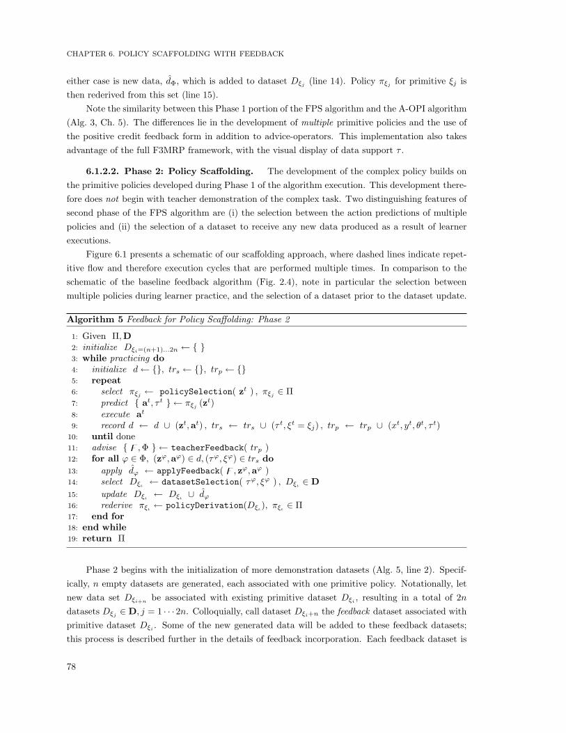
CHAPTER 6. POLICY SCAFFOLDING WITH FEEDBACK
either case is new data, dΦ, which is added to dataset Dξj (line 14). Policy πξj for primitive ξj isthen rederived from this set (line 15).
Note the similarity between this Phase 1 portion of the FPS algorithm and the A-OPI algorithm(Alg. 3, Ch. 5). The differences lie in the development of multiple primitive policies and the use ofthe positive credit feedback form in addition to advice-operators. This implementation also takesadvantage of the full F3MRP framework, with the visual display of data support τ .
6.1.2.2. Phase 2: Policy Scaffolding. The development of the complex policy builds onthe primitive policies developed during Phase 1 of the algorithm execution. This development there-fore does not begin with teacher demonstration of the complex task. Two distinguishing features ofsecond phase of the FPS algorithm are (i) the selection between the action predictions of multiplepolicies and (ii) the selection of a dataset to receive any new data produced as a result of learnerexecutions.
Figure 6.1 presents a schematic of our scaffolding approach, where dashed lines indicate repet-itive flow and therefore execution cycles that are performed multiple times. In comparison to theschematic of the baseline feedback algorithm (Fig. 2.4), note in particular the selection betweenmultiple policies during learner practice, and the selection of a dataset prior to the dataset update.
Algorithm 5 Feedback for Policy Scaffolding: Phase 2
1: Given Π,D2: initialize Dξi=(n+1)...2n ← { }3: while practicing do4: initialize d← {}, trs ← {}, trp ← {}5: repeat6: select πξj ← policySelection( zt ) , πξj ∈ Π7: predict { at, τ t } ← πξj (zt)8: execute at
9: record d ← d ∪ (zt,at) , trs ← trs ∪ (τ t, ξt = ξj) , trp ← trp ∪ (xt, yt, θt, τ t)10: until done11: advise { z,Φ } ← teacherFeedback( trp )12: for all ϕ ∈ Φ, (zϕ,aϕ) ∈ d, (τϕ, ξϕ) ∈ trs do13: apply dϕ ← applyFeedback( z, zϕ,aϕ )14: select Dξι ← datasetSelection( τϕ, ξϕ ) , Dξι ∈ D15: update Dξι ← Dξι ∪ dϕ16: rederive πξι ← policyDerivation(Dξι), πξι ∈ Π17: end for18: end while19: return Π
Phase 2 begins with the initialization of more demonstration datasets (Alg. 5, line 2). Specif-ically, n empty datasets are generated, each associated with one primitive policy. Notationally, letnew data set Dξi+n be associated with existing primitive dataset Dξi , resulting in a total of 2ndatasets Dξj ∈ D, j = 1 · · · 2n. Colloquially, call dataset Dξi+n the feedback dataset associated withprimitive dataset Dξi . Some of the new generated data will be added to these feedback datasets;this process is described further in the details of feedback incorporation. Each feedback dataset is
78

6.1 ALGORITHM: FEEDBACK FOR POLICY SCAFFOLDING
Figure 6.1. Policy derivation and execution under the Feedback for Policy Scaffolding algorithm.
treated identically to the primitive datasets during policy execution. That is, a policy is derivedfrom each feedback dataset, and these policies are considered for selection during execution of themore complex policy.
During the learner execution portion of the practice run (lines 5-10), the learner executes withthe complex policy. At each decision cycle, the operation of this policy proceeds in two steps. Thefirst step is to select between all contributing policies πξj based on observation zt (line 6); the detailsof this selection are provided in Section 6.1.3.1. The second step is to predict action at according toπξj (z
t), with prediction support τ t (line 7). The selected action is executed. A variety of informationis then recorded (line 9). The action at is recorded in the prediction trace d, along with observationzt. The measure of data support τ t for the prediction and a tag ξj indicating the selected policyare recorded into the selection trace trs, which will be utilized during the selection of a datasetto receive feedback-modified data. The learner position and heading within the world (xt, yt, θt) isrecorded along with the prediction support τ t into the position trace trp, for use during the F3MRPgraphical display for the teacher.
79

CHAPTER 6. POLICY SCAFFOLDING WITH FEEDBACK
During the teacher feedback and policy update portion of a practice run (lines 11-17), theadvisor first indicates a segment Φ, of the learner execution, and provides feedback z for thatsegment. As in Phase 1, two feedback forms are available: binary credit, z ≡ c, and correctiveadvice, z ≡ op.
The teacher feedback is then applied across all points within the indicated subset Φ. For eachselected execution point, indexed as ϕ ∈ Φ, the first step is to apply feedback z to the point (zϕ,aϕ)recorded in d (line 13). The next step is to select one of the datasets to receive this data (line 14).Specifically, dataset Dξι is selected, based on the recorded data support τϕ and tag ξϕ associatedwith the execution point; the details of this selection are provided in Section 6.1.3.2. The selecteddataset is updated with the feedback-modified data point (line 15) and the policy πξι associatedwith this dataset is rederived (line 16).
6.1.3. Scaffolding Multiple Policies
One key factor when building a policy from simpler behaviors is how to select between thebehaviors. A second key factor is how to incorporate teacher feedback into the built-up policy. Thedesign of each of these factors within the FPS algorithm are discussed here. Later sections (6.3.2.1and 6.3.2.2 respectively) discuss a few of the iterative stages from the development of these factors.
6.1.3.1. Selecting Primitive Policies. Primitive selection assumes that primitives occupynominally distinct areas of the observation-space. This assumption relies on the state observationformulation capturing aspects of the world that are unique to the demonstrations of each primitivepolicy. For example, in the following section two of the primitives developed for a racetrack drivingtask are turn left and turn right. Demonstrations of the turn left primitive occur in areas of thetrack that curve to the left, and of turn right in areas that curve to the right. Observations areformulated to incorporate a notion of track curvature, and so the demonstrations for each primitiveoccupy distinct areas of the observation-space.
Primitive selection then is treated as a classification problem. For each primitive ξj , a kernelizeddistance φ (zt, zi) = e|zi−zt|Σ−1|zi−zt| is computed between query point zt and each point zi ∈ Dξj .The distance computation is Euclidean and the kernel Gaussian. The parameter Σ−1 is a constantdiagonal matrix that scales each observation dimension and embeds the bandwidth of the Gaussiankernel. This parameter is tuned through 10-folds Cross Validation to optimize the least squarederror on primitive label classification. A weight for policy ξj is computed by summing the k largestkernel values φ (zt, :) computed between zt and the points within Dξj ; equivalent to selecting thek−nearest points in Dξj to query zt (k = 5). A weight is similarly computed for all primitivesξj ∈ Ξ, and the primitive ξj with the highest weight is then selected.
6.1.3.2. Incorporating Teacher Feedback. The FPS algorithm produces data fromteacher feedback on policy executions with multiple primitive policies. A variety of options exist forhow to then incorporate this data into the multiple underlying datasets.
To begin, let us establish two ideas. First, this work assumes that in state-space areas coveredby the dataset of a particular primitive, the behavior of this primitive matches the intended behaviorof the more complex policy. If this is not the case, and the two behaviors conflict, then that primitive
80

6.2 EMPIRICAL SIMULATION IMPLEMENTATION
should not be incorporated into the complex policy in the first place. Second, the feedback formsconsidered in this chapter both produce new data. The new data derives from learner executions,such that every new datapoint dϕ = (zϕ, aϕ) derives from an execution point (zϕ,aϕ). Each learnerexecution point is predicted by a single primitive policy, as discussed in the previous section.
Two factors determine into which dataset a new datapoint dϕ is added: the policy ξϕ thatpredicted the execution point (zϕ,aϕ), and the measure of data support τϕ for that prediction. Inparticular, if the policy that made the prediction is a primitive policy, the point is added to itsdataset if the prediction had strong data support. Otherwise, the point is added to the feedbackdataset associated with primitive ξϕ (Sec. 6.1.2.2). By contrast, data generated from executionpoints predicted by a feedback policy are automatically added to its dataset, regardless of datasetsupport.
This idea of prediction data support is the same as that used by the F3MRP feedback interfacewhen providing the teacher with a visual representation of the measure of data support for predic-tions, as described in Chapter 2 (Sec. 2.3.2.1). Each primitive ξj therefore has an associated Poissondistribution, parameterized by λξj modeling the distribution of 1−NN distances between points inDξj , with mean µξj = λξj and standard deviation σj =
√λξj . We set by hand the threshold on
strong prediction support to be τj = µξj + 5σξj , based on empirical evidence. Thus a predictionmade by policy πξj for query point zt with distance `zt to the nearest point in Dξj is classified asstrongly supported if `zt < τξj and weakly supported otherwise.
The motivation behind this approach is to avoid adding data to the primitive datasets thatconflicts with the primitive behavior. We assume that observations near to points in a primitivedataset have an associated behavior that does not conflict with the intended behavior of the primitivedataset. Therefore points that were close enough to be strongly supported during their associatedaction prediction exhibit a similar behavior.
6.2. Empirical Simulation Implementation
This section presents results from the application of the FPS algorithm to a simulated motioncontrol domain. Motion control primitives are learned for a racetrack driving task, and are scaffoldedinto a policy able to perform the full task. Furthermore, all FPS policies are found to outperformthose developed under the typical approach of providing more teacher demonstrations.
6.2.1. Experimental Setup
Here we present the experimental details, beginning with the task and domain, and followed bya description of the various policies developed for empirical evaluation.
6.2.1.1. Racetrack Driving Task and Domain. The domain chosen to validate the FPSpolicy building algorithm is a simulated differential drive robot within a racetrack driving domain.The task consists of the robot driving along a racetrack, with two failure criteria: the robot eitherstops moving or crosses a track boundary. The dimensions and parameters set in this simulateddomain derive from real world execution with a Segway RMP robot. Robot motion is propagated
81
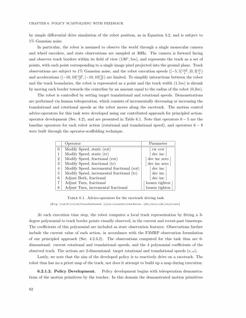
CHAPTER 6. POLICY SCAFFOLDING WITH FEEDBACK
by simple differential drive simulation of the robot position, as in Equation 3.2, and is subject to1% Gaussian noise.
In particular, the robot is assumed to observe the world through a single monocular cameraand wheel encoders, and state observations are sampled at 30Hz. The camera is forward facingand observes track borders within its field of view (130◦, 5m), and represents the track as a set ofpoints, with each point corresponding to a single image pixel projected into the ground plane. Trackobservations are subject to 1% Gaussian noise, and the robot execution speeds ([−5, 5] rads , [0, 3]ms )and accelerations ([−10, 10] rads2 , [−10, 10]ms2 ) are limited. To simplify interactions between the robotand the track boundaries, the robot is represented as a point and the track width (1.5m) is shrunkby moving each border towards the centerline by an amount equal to the radius of the robot (0.3m).
The robot is controlled by setting target translational and rotational speeds. Demonstrationsare performed via human teleoperation, which consists of incrementally decreasing or increasing thetranslational and rotational speeds as the robot moves along the racetrack. The motion controladvice-operators for this task were developed using our contributed approach for principled action-operator development (Sec. 4.2), and are presented in Table 6.1. Note that operators 0− 5 are thebaseline operators for each robot action (rotational and translational speed), and operators 6 − 8were built through the operator-scaffolding technique.
Operator Parameter0 Modify Speed, static (rot) [ cw ccw ]1 Modify Speed, static (tr) [ dec inc ]2 Modify Speed, fractional (rot) [ dec inc zero ]3 Modify Speed, fractional (tr) [ dec inc zero ]4 Modify Speed, incremental fractional (rot) [ dec inc ]5 Modify Speed, incremental fractional (tr) [ dec inc ]6 Adjust Both, fractional [ dec inc ]7 Adjust Turn, fractional [ loosen tighten ]8 Adjust Turn, incremental fractional [ loosen tighten ]
Table 6.1. Advice-operators for the racetrack driving task.
[Key: (rot/tr)=(rot/transl)ational, (c)cw=(counter)clockwise, (dec/inc)=(de/in)crease]
At each execution time step, the robot computes a local track representation by fitting a 3-degree polynomial to track border points visually observed, in the current and recent-past timesteps.The coefficients of this polynomial are included as state observation features. Observations furtherinclude the current value of each action, in accordance with the F3MRP observation formulationof our principled approach (Sec. 4.2.3.2). The observations computed for this task thus are 6-dimensional: current rotational and translational speeds, and the 4 polynomial coefficients of theobserved track. The actions are 2-dimensional: target rotational and translational speeds (ν, ω).
Lastly, we note that the aim of the developed policy is to reactively drive on a racetrack. Therobot thus has no a priori map of the track, nor does it attempt to build up a map during execution.
6.2.1.2. Policy Development. Policy development begins with teleoperation demonstra-tions of the motion primitives by the teacher. In this domain the demonstrated motion primitives
82

6.2 EMPIRICAL SIMULATION IMPLEMENTATION
(Fig. 6.2) are: turn right (ξR), go straight (ξS), turn left (ξL). The steps taken by the FPS algorithmduring policy development are to:
1. Demonstrate the motion primitives, and derive initial policies.
2. Provide feedback on the motion primitive policies’ performance.
3. Derive an initial scaffolded policy from the resultant primitive policies.
4. Provide feedback on the scaffolded policy performance.
Demonstration of each primitive behavior is performed 3 times from a single location on thetrack appropriate for the associated primitive motion, for a total of 9 demonstrations (dataset sizes:|DξR | = 297, |DξS | = 154, and |DξL | = 245 points, summed datasets’ size: 696 points). An initialpolicy is derived from each of these datasets; we refer to these collectively as the set of initialdemonstrated primitive policies, PDI .
Next the learner executes with each policy in PDI , on a subset of the track correspondingto the respective location of the primitive behavior’s demonstrations. The teacher observes theseexecutions, offers feedback, and the executing policy is updated. Data generated from teacherfeedback on executions with a given policy ξi is added to the respective primitive dataset Dξi (i =R,S, L). This observation-feedback -update cycle constitutes a single practice run, and continues tothe satisfaction of the teacher. Final feedback versions of the primitive policies are the result of thisfirst phase of feedback. We refer to the collection of these policies as the final feedback primitivepolicies, PFF (summed datasets’ size: 1, 835 point).
The learner then builds a policy able to execute a more complex behavior; that is, able to executeon the full racetrack. A baseline scaffolded policy, that operates by selecting between the primitivepolicies in PFF , is built; we refer to this as the initial feedback scaffolded policy, SFI . The learnerexecutes with this policy on the full track. Again these executions are observed by the teacher,and the observation-feedback-update cycle continues to her satisfaction. Here, data generated fromfeedback is added to either the primitive datasets or their respective feedback datasets, accordingto the paradigm described in Section 6.1.3.2. The final feedback scaffolded policy SFF is the resultfrom this second phase of feedback (summed datasets’ size: 6, 438 points).
For comparative purposes, the approach of providing exclusively teacher demonstrations is alsoevaluated. This approach closely follows the advising approach just outlined, but the teacher providesmore teleoperation demonstrations instead of feedback. In response to learner executions with theinitial primitive policies in PDI , the learner is provided with more motion primitive demonstrations.This observation-demonstration-update cycle constitutes a single practice run, and continues to thesatisfaction of the teacher. These demonstrations are added to the respective datasets for eachprimitive. Final demonstration versions of the primitive policies are the result. We refer to thecollection of these policies as the final demonstration primitive policies, PDF (summed datasets’ size:4, 608 points). A baseline scaffolded policy is then built from the these primitive policies; we refer tothis policy as the initial scaffolded demonstration policy SDI . In response to learner executions withpolicy SDI on the full track, the teacher provides full track teleoperation demonstrations. Thesedemonstrations are added to a new dataset, from which a policy is derived that also is considered
83

CHAPTER 6. POLICY SCAFFOLDING WITH FEEDBACK
during execution of the scaffolded policy. The result is the final scaffolded demonstration policySDF (summed datasets’ size: 14, 657 points).
To summarize, a total of 13 policies are developed for empirical evaluation:
Primitive, Demonstration Initial (PDI) : Initial demonstration of each primitive (3 in total)Primitive, Feedback Final (PFF ) : Feedback for PDI (3 in total)Primitive, Demonstration Final (PDF ) : More demonstration for PDI (3 in total)
Scaffolded, Feedback Initial (SFI) : Initial scaffolding of the PFF policiesScaffolded, Feedback Final (SFF ) : Feedback for SFI
Scaffolded, Demonstration Initial (SDI) : Initial scaffolding of the PDF policiesScaffolded, Demonstration Final (SDF ) : More demonstration for SDI
6.2.1.3. Evaluation. Each of the developed policies are evaluated on racetrack executions.In particular, each of the primitive policies (contained in sets PDI , PFF , PDF ) is evaluated on thetrack subset appropriate to their respective primitive behavior (Fig. 6.2, left). Each of the scaffoldedpolicies (SFI , SFF , SDI , SDF ) is evaluated on the full track (Fig. 6.2, right). Executions proceedalong the track and end when the robot either runs off the track or reaches the finish line.
Figure 6.2. Primitive subset regions (left) of the full racetrack (right).
Policy performance is measured according to the following metrics. Success indicates the abilityof the robot to stay on the track, and is measured by the percentage of the track subset (for primitivepolicy executions) or full track (for scaffolded policy executions) completed. Speed is measured bythe average translational execution speed. Efficiency is measured as the execution time, and isgoverned jointly by speeds and the execution ground path. This measure is computed for successfulexecutions exclusively; for unsuccessful executions, that by definition aborted early, time is not auseful measure.
84
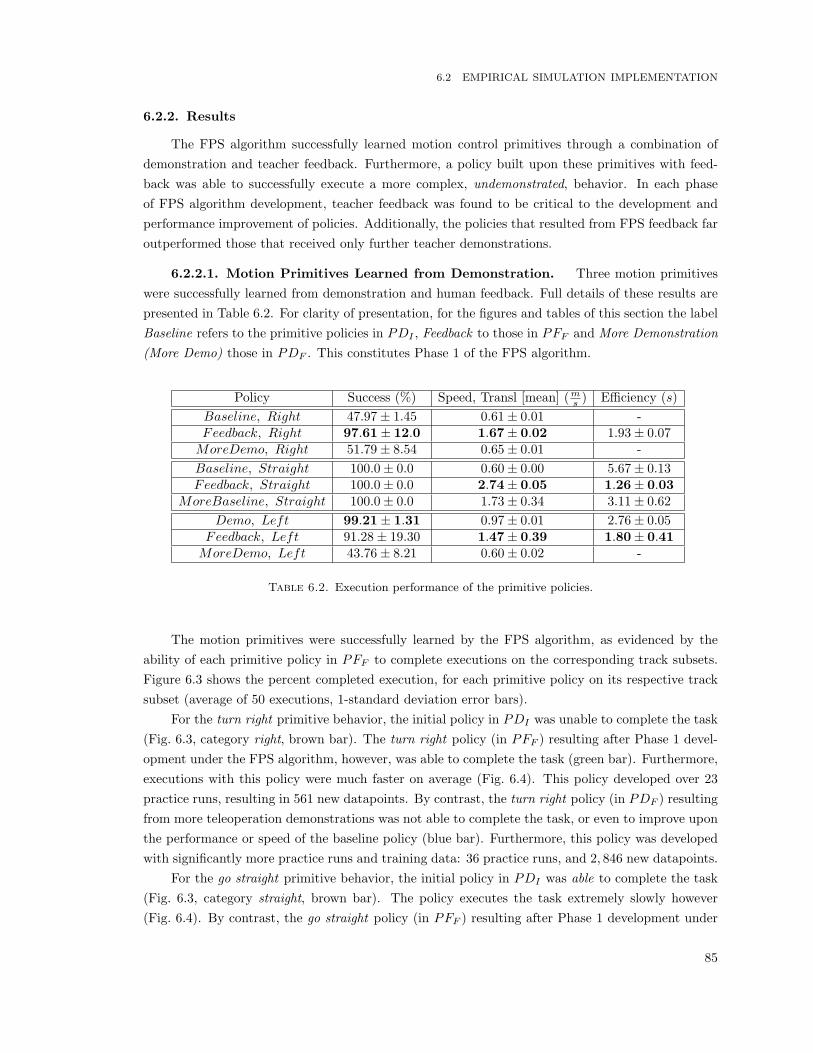
6.2 EMPIRICAL SIMULATION IMPLEMENTATION
6.2.2. Results
The FPS algorithm successfully learned motion control primitives through a combination ofdemonstration and teacher feedback. Furthermore, a policy built upon these primitives with feed-back was able to successfully execute a more complex, undemonstrated, behavior. In each phaseof FPS algorithm development, teacher feedback was found to be critical to the development andperformance improvement of policies. Additionally, the policies that resulted from FPS feedback faroutperformed those that received only further teacher demonstrations.
6.2.2.1. Motion Primitives Learned from Demonstration. Three motion primitiveswere successfully learned from demonstration and human feedback. Full details of these results arepresented in Table 6.2. For clarity of presentation, for the figures and tables of this section the labelBaseline refers to the primitive policies in PDI , Feedback to those in PFF and More Demonstration(More Demo) those in PDF . This constitutes Phase 1 of the FPS algorithm.
Policy Success (%) Speed, Transl [mean] (ms ) Efficiency (s)Baseline, Right 47.97± 1.45 0.61± 0.01 -Feedback, Right 97.61± 12.0 1.67± 0.02 1.93± 0.07MoreDemo, Right 51.79± 8.54 0.65± 0.01 -Baseline, Straight 100.0± 0.0 0.60± 0.00 5.67± 0.13Feedback, Straight 100.0± 0.0 2.74± 0.05 1.26± 0.03
MoreBaseline, Straight 100.0± 0.0 1.73± 0.34 3.11± 0.62Demo, Left 99.21± 1.31 0.97± 0.01 2.76± 0.05
Feedback, Left 91.28± 19.30 1.47± 0.39 1.80± 0.41MoreDemo, Left 43.76± 8.21 0.60± 0.02 -
Table 6.2. Execution performance of the primitive policies.
The motion primitives were successfully learned by the FPS algorithm, as evidenced by theability of each primitive policy in PFF to complete executions on the corresponding track subsets.Figure 6.3 shows the percent completed execution, for each primitive policy on its respective tracksubset (average of 50 executions, 1-standard deviation error bars).
For the turn right primitive behavior, the initial policy in PDI was unable to complete the task(Fig. 6.3, category right, brown bar). The turn right policy (in PFF ) resulting after Phase 1 devel-opment under the FPS algorithm, however, was able to complete the task (green bar). Furthermore,executions with this policy were much faster on average (Fig. 6.4). This policy developed over 23practice runs, resulting in 561 new datapoints. By contrast, the turn right policy (in PDF ) resultingfrom more teleoperation demonstrations was not able to complete the task, or even to improve uponthe performance or speed of the baseline policy (blue bar). Furthermore, this policy was developedwith significantly more practice runs and training data: 36 practice runs, and 2, 846 new datapoints.
For the go straight primitive behavior, the initial policy in PDI was able to complete the task(Fig. 6.3, category straight, brown bar). The policy executes the task extremely slowly however(Fig. 6.4). By contrast, the go straight policy (in PFF ) resulting after Phase 1 development under
85

CHAPTER 6. POLICY SCAFFOLDING WITH FEEDBACK
Primitive Policy Success
Figure 6.3. Percent task completion with each of the primitive behavior policies.
the FPS algorithm was able to increase execution speeds (green bar), such that the average speedover the execution approaches the maximum speed of the robot (3.0ms ), all without compromisingthe success of the executions. This policy developed over 27 practice runs, resulting in 426 newdatapoints. The go straight policy (in PDF ) resulting from more teleoperation demonstrations alsoimproved execution speeds over the baseline policy, but not as dramatically (blue bar). This policydeveloped over 36 practice runs, resulting in 1, 630 new datapoints.
Primitive Policy Speed
Figure 6.4. Average translational execution speed with each of the primitive behavior policies.
86
6.2 EMPIRICAL SIMULATION IMPLEMENTATION
For the turn left primitive behavior, the initial policy in PDI again was able to complete thetask (Fig. 6.3, category left, brown bar). The turn left policy (in PFF ) resulting after Phase 1 devel-opment under the FPS algorithm also was able complete the task (green bar), though occasionallydid go off the track (Fig. 6.3). This was a consequence of the policy being more aggressive than thebaseline policy, as evidenced by its increased execution speeds (Fig. 6.4, category left, green bar).The advantage of this aggression was much more efficient executions (Tbl. 6.2, Feedback, Left), butat the cost of occasional incomplete executions. This policy developed over 8 practice runs, resultingin 252 new data points. The turn left policy (in PDF ) resulting from more teleoperation demonstra-tions actually decreased the performance of the initial policy, both in success and speed (blue bar).Presumably more demonstrations in this case created ambiguous areas for the policy, a complicationthat would perhaps clear up with the presentation of more disambiguating demonstrations. Thispolicy developed over 12 practice runs, resulting in 965 new datapoints.
6.2.2.2. Undemonstrated Task Learned from Primitives and Feedback. A policyable to execute a more complex, undemonstrated, behavior was successfully developed through thescaffolding of the learned primitive policies and the incorporation of teacher feedback. The complextask here is the robot driving on the full racetrack. Before any practice runs with teacher feedback,the complex policy, derived solely from selection between the developed feedback primitive policiesPFF , was unable to execute this task in full. Performance improvement over 160 practice runsis presented in Figure 6.5. Each practice run produces a new iterative policy. Each plot pointrepresents an average of 10 track executions with a given iterative policy, and a regularly sampledsubset of the iterative policies were evaluated in this manner (sampled every 10 policies, 17 iterativepolicies evaluated in total). This constitutes Phase 2 of the FPS algorithm, after which the learnerwas able to consistently execute the complex task in full.
Complex Policy Success, Improvement with Practice
Figure 6.5. Percent task completion during complex policy practice.
87

CHAPTER 6. POLICY SCAFFOLDING WITH FEEDBACK
6.2.2.3. Improvement in Complex Task Performance. Beyond the development ofa policy able to perform the more complex task, Phase 2 of the FPS algorithm further enabledperformance improvement such that task executions became faster and more efficient. Figure 6.6shows the percent completed execution of multiple policies on the full track task (average of 50executions, 1-standard deviation error bars); further details of these results are presented in Table 6.3.
Complex Policy Success
Figure 6.6. Percent task completion with full track behavior policies.
As noted above, the initial FPS policy SFI , derived exclusively from the primitive feedbackpolicies in PFF , was not able to complete this task (Fig. 6.6, Feedback Initial). Neither was theinitial policy SDI derived exclusively from the primitives in PDF developed from more teacherdemonstrations (Demo Initial). Both of these policies performed similarly poorly in the measure ofexecution success.
The final policy SFF that resulted after Phase 2 of the FPS algorithm, however, was able toconsistently execute the task successfully (Fig. 6.6, Feedback Final). This policy developed over 160practice runs, resulting in 4, 503 new datapoints. By contrast, the policy SDF that resulted frommore teleoperation demonstrations (Demo Final) was not able to complete the task, though it didimprove upon the performance the initial demonstration policy (Demo Initial). The policy SDF
developed over 75 practice runs, resulting in 8, 520 new datapoints.Policy development terminated at the discretion of the feedback teacher. In general the teacher
decided to terminate development once a policy displayed either satisfactory performance or nofurther performance improvement. In the development of final demonstration policy SDF , however,the teacher aborted policy development due to her frustration with the extremely slow rate of policyimprovement. Since the final FPS policy SFF received feedback on more practice runs than the moredemonstration policy SDF (159 vs. 74), the above comparison between these policies is not a fairone. To provide a fair comparison, results from an iterative FPS policy are also presented (Fig. 6.6,Feedback* ). This policy is not the final FPS policy, but rather the result of development afteronly 74 practice runs, the same number of practice runs as the final demonstration policy. Theseruns produced 2, 448 new datapoints; far fewer than the 74 runs of the demonstration policy, which
88

6.2 EMPIRICAL SIMULATION IMPLEMENTATION
produced 8, 520 new points. Against this iterative policy also, however, the final demonstrationpolicy did not measure well. The iterative policy (Feedback* ) significantly outperformed the finaldemonstration policy (Demo Final) on the success measure, though it does not yet perform assuccessfully or as consistently as the final FPS policy (Feedback Final).
Policy Success (%) Speed, Transl [mean, max] (ms ) Speed, Rot [max] ( rads )Feedback Initial 6.32± 1.72 0.42± 0.21 , 1.51± 0.36 0.88± 0.3
Feedback∗ 63.32± 28.49 2.24± 0.18 , 3.04± 0.17 2.14± 0.2Feedback F inal 97.51± 7.94 2.34± 0.03 , 3.07± 0.01 2.57± 0.06Demo Initial 5.95± 0.17 0.58± 0.00 , 0.66± 0.13 0.15± 0.10Demo Final 13.69± 2.36 1.01± 0.13 , 1.51± 0.56 0.98± 0.14
Table 6.3. Execution performance of the scaffolded policies.
Policies were additionally evaluated for speed, the results of which are presented in Figure 6.7.Since the full track is much longer than any of the primitive subsets, and thus offers more opportunityto reach higher speeds, the maximum speeds attained during executions are shown in addition tothe average speed.
The speed performance results closely resemble those of success performance. Namely, the finalFPS policy (Feedback Final) far outperformed both the initial FPS policy (Feedback Initial) as wellas the final demonstration policy (Demo Final). The final demonstration policy did offer someimprovement over the initial demonstration policy (Demo Initial), but not nearly as much as theiterative FPS policy provided for comparison (Feedback∗). Interesting to note is that this iterativeFPS policy produced speeds similar to the final FPS in nearly all measures, though with slightlylarger standard deviations (Tbl. 6.3). This suggests that the motivations for continuing practice anddevelopment beyond this iterative policy included performance consistency, in addition to executionsuccess.
6.2.2.4. Appropriate Behavior Selection. Under FPS, the demonstration teacher pro-vides no explicit indication of circumstances in which the behavior of a given primitive is suitablefor the complex task. Instead, the algorithm selects between behavior primitives based solely on thedistribution of their data within the observation space. In this section we show that this selectionparadigm did in fact choose behavior that was appropriate for the various portions of the complextask execution.
Figure 6.8 shows examples of primitive policy selection, during full track executions with thefinal FPS policy SFF . Five example executions are shown as panels A-E. Across a panel, a singleexecution trace is displayed in triplicate, with each plot corresponding to the selection of a differentpolicy primitive. Within a single plot, execution points for which the given behavior policy wasselected are displayed as blue circles, and those for which the primitive behavior’s associated feedbackpolicy was selected are displayed as red circles. For reference, the full execution trace is displayedas well (cyan line). Each execution begins at the track start line (green line, lower right corner) and
89

CHAPTER 6. POLICY SCAFFOLDING WITH FEEDBACK
Complex Policy Speed
Figure 6.7. Average and maximum translational (top) and rotational (bottom) speedswith full track behavior policies.
ends at either the finish line (magenta line, upper left corner) or the point at which the robot droveoff the track (e.g. panel C).
A macro-level analysis across each panel confirms the correct selection of primitive policiesoverall; namely that in right-turn areas of the track the right behavior was selected, in straight areasthe straight behavior was selected and in left-turn areas the left behavior was selected.
Upon closer inspection, interesting differences between policy selections are discernible. Forexample, in the right-turn track areas, across all panels the right-feedback policy is seldom selected(red circles, first column); by contrast the straight-feedback and left-feedback policies are frequentlyselected in their respective track areas (red circles, second and third columns). There are threepossible algorithmic explanations for this low selection frequency. One: Predictions made by theright policy never received teacher feedback. Two: The right policy predictions did receive teacherfeedback, but were rarely predicting in areas of the state-space outside the support threshold τ
for the right policy. Both of these reasons would result in the right-feedback dataset receiving few
90

6.2 EMPIRICAL SIMULATION IMPLEMENTATION
datapoints and consequently having very limited data support. Three: The behavior of the complextask policy developed in such a way that it no longer visited the state-space areas that populate theright-feedback dataset. In this particular case of these experiments, the second reason accounts forthe low selection frequency.
RIGHT STRAIGHT LEFT
(A)
(B)
(C)
(D)
(E)
Figure 6.8. Example complex driving task executions (rows), showing primitive behaviorselection (columns), see text for details.
91
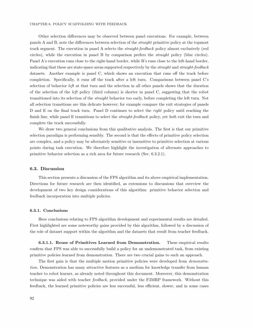
CHAPTER 6. POLICY SCAFFOLDING WITH FEEDBACK
Other selection differences may be observed between panel executions. For example, betweenpanels A and B, note the differences between selection of the straight primitive policy at the topmosttrack segment. The execution in panel A selects the straight-feedback policy almost exclusively (redcircles), while the execution in panel B by comparison prefers the straight policy (blue circles).Panel A’s execution runs close to the right-hand border, while B’s runs close to the left-hand border,indicating that these are state-space areas supported respectively by the straight and straight-feedbackdatasets. Another example is panel C, which shows an execution that runs off the track beforecompletion. Specifically, it runs off the track after a left turn. Comparisons between panel C’sselection of behavior left at that turn and the selection in all other panels shows that the durationof the selection of the left policy (third column) is shorter in panel C, suggesting that the robottransitioned into its selection of the straight behavior too early, before completing the left turn. Notall selection transitions are this delicate however; for example compare the exit strategies of panelsD and E on the final track turn. Panel D continues to select the right policy until reaching thefinish line, while panel E transitions to select the straight-feedback policy, yet both exit the turn andcomplete the track successfully.
We draw two general conclusions from this qualitative analysis. The first is that our primitiveselection paradigm is performing sensibly. The second is that the effects of primitive policy selectionare complex, and a policy may be alternately sensitive or insensitive to primitive selection at variouspoints during task execution. We therefore highlight the investigation of alternate approaches toprimitive behavior selection as a rich area for future research (Sec. 6.3.2.1).
6.3. Discussion
This section presents a discussion of the FPS algorithm and its above empirical implementation.Directions for future research are then identified, as extensions to discussions that overview thedevelopment of two key design considerations of this algorithm: primitive behavior selection andfeedback incorporation into multiple policies.
6.3.1. Conclusions
Here conclusions relating to FPS algorithm development and experimental results are detailed.First highlighted are some noteworthy gains provided by this algorithm, followed by a discussion ofthe role of dataset support within the algorithm and the datasets that result from teacher feedback.
6.3.1.1. Reuse of Primitives Learned from Demonstration. These empirical resultsconfirm that FPS was able to successfully build a policy for an undemonstrated task, from existingprimitive policies learned from demonstration. There are two crucial gains to such an approach.
The first gain is that the multiple motion primitive policies were developed from demonstra-tion. Demonstration has many attractive features as a medium for knowledge transfer from humanteacher to robot learner, as already noted throughout this document. Moreover, this demonstrationtechnique was aided with teacher feedback, provided under the F3MRP framework. Without thisfeedback, the learned primitive policies are less successful, less efficient, slower, and in some cases
92

6.3 DISCUSSION
even unable to complete the target behavior. This is true not just of the initial primitive policies de-rived from demonstration, but also of the policies provided with more demonstrations in response tolearner execution performance. The FPS algorithm therefore provides a more efficient and effectiveLfD technique for the development of these motion primitive policies.
Even with the advantages secured through demonstration and teacher feedback however, policydevelopment typically is still a non-trivial task. The second gain of the FPS approach thereforeis the ability to reuse the primitives within another policy. The full track task was shown to besufficiently complex that the improvements afforded by demonstrations of the full task behaviorwere significantly smaller than those gained through teacher feedback. Moreover, this performancedifference between the feedback and more-demonstration techniques was much larger for the complextask than for the simpler primitive policies (compare Figs. 6.3 and 6.6). These figures suggestthat the complex task would not be learned through demonstration exclusively, i.e. from full taskdemonstrations alone, unless provided with a very large quantity of demonstration data, againunderlining the advantage of simple policy reuse within this complex domain.
6.3.1.2. Feedback Incorporation based on Data Support. One core idea in the FPSfeedback framework is the measure of data support associated with policy predictions. This measureis employed in two distinct steps of the feedback framework operation.
Data support is first considered by the teacher when selecting feedback for a given learnerexecution. The graphical display of the F3MRP interface provides the teacher with an idea ofdata support throughout the execution. Segments of the execution that correspond jointly to goodperformance and weak data support are selected to receive positive credit feedback from the teacher.The data support measure in this case drives both where and what type of feedback is provided.Since this feedback produces new data, the support measure consequently also drives the generationof new demonstration examples.
Prediction data support is next used by the learner when selecting which dataset receives newfeedback-generated data. One of the research questions considered in this thesis is how to incorporateteacher feedback into complex tasks. The idea of data-supported predictions is fundamental tothe feedback incorporation approach taken in the FPS algorithm. The intent here is to maintainthe performance integrity of the learned primitive behaviors. The data support measure in thiscase guides policy development, both of the primitive behavior policies, as well as their associatedprimitive-feedback policies, whose datasets receive those points deemed unsuitable for, i.e. distantfrom, the primitive behavior datasets.
6.3.1.3. Even More Focused Datasets. One result of the A-OPI experimental valida-tions was the development of much smaller datasets with corrective advice in comparison to moredemonstrations (Sec. 5.3.2.2). These smaller datasets furthermore produced similar or superiorperformance, prompting the conclusion that the data contained in the A-OPI datasets was lessredundant and more focused.
This trend is also seen with the FPS datasets of this work, and appears to only magnify withthe more complex task of this domain. In particular, the combined size of the three primitivepolicy datasets developed with more demonstration (6, 137) is more than three times the size of
93
CHAPTER 6. POLICY SCAFFOLDING WITH FEEDBACK
the comparable FPS primitive datasets (1, 935) and in fact is on par with the size of the finalFPS scaffolded policy (6, 438). The size of the final scaffolded more-demonstration policy dataset(14, 657) is more than double the final FPS dataset size, and this is with far fewer practice runs(74 vs. 168) The size of the comparable iterative FPS dataset (4, 383) is less than a third of the finaldemonstration dataset.
In contrast to the Chapter 5 results however, these teleoperation policies never perform similarlyto their FPS counterparts, and instead usually display significantly inferior performance. This ob-servation suggests that not only is the added data less redundant, but furthermore includes relevantdata that is not being produced by the demonstration. In particular, revisiting states to demon-strate a correct behavior is difficult with motion control tasks, and this difficulty scales with taskcomplexity. The difficulty in revisiting states was noted by the feedback teacher when attempting toprovide corrective demonstrations for primitive executions on the track subsets, and only increasedwith the full track executions when revisiting execution states even approximately became nearlyimpossible. Further detrimental to the developed policies was the fact that the teacher often wasrequired to reproduce suboptimal behavior in order to reach the state intended to receive a correc-tive demonstration. The result was that poor demonstration data was provided to the learner, inaddition to the behavior correction in the target area. While there do exist a handful of algorithmsthat explicitly address bad demonstrations (see Sec. 9.1.3), this is not typical of LfD in general andfurthermore was not the focus of this work.
In contrast to all of the difficulties associated with revisiting state, policy improvement underthe F3MRP framework does not require revisiting any states in order to provide feedback. Wepropose that the value of this key advantage of the F3MRP framework only grows as tasks anddomains become more complex.
6.3.2. Future Directions
This section provides ideas for the extension and improvement of the FPS algorithm. Thepresentation is framed within a discussion of two key design decisions for this algorithm: how toselect between primitive behaviors, and how to incorporate teacher feedback into the complex policy.
6.3.2.1. Primitive Behavior Selection. The initial version of the algorithm performedno explicit primitive selection. Instead, this implementation relied exclusively on the local nature ofthe employed regression techniques, and the assumption that primitives occupy distinct areas of thestate-space. Demonstrations of all primitive behaviors were pooled into a single dataset. LocallyWeighted Learning regression techniques consider only nearby data in the regression prediction.Since all nearby data was assumed to result from demonstrations of the same primitive, when oper-ating in the state-space area of a particular primitive the regression technique in theory incorporatesdata from a single primitive only, and thus implicitly performs primitive selection.
The performance of this implicit primitive selection, however, was found to be substandard.Though primitives do occupy nominally distinct areas of the state-space, the implicit primitive se-lection paradigm relied on the stronger assumption of no overlap between these areas. Violations of
94
6.3 DISCUSSION
this assumption resulted in the mixing of data from different primitives into a single regression pre-diction, and consequently poor performance in regions of primitive data overlap. Poor performancewill result if the actions of different behavior primitives conflict, for example if the rotational speedof 1.0 rads for primitive turn left versus 1.0 rads for turn right become a mixed action prediction thatdoes not turn at all, 0.0 rads = 1
2 (1.0 rads ) + 12 (−1.0 rads ).
The next algorithm version therefore relaxed the assumption of non-overlapping state-spacesbetween primitives. Datapoints were restricted to make predictions only with other points of thesame primitive type; effectively isolating demonstrations of a particular primitive type into separatedatasets, and treating each primitive as its own policy. This implementation then performed explicitprimitive selection at execution time based on query point nearness, by selecting the primitive withthe dataset containing the nearest point to the query point.
A more robust version of this implementation is included in the final version of the algorithm.Primitives similarly are treated as individual policies, and primitive selection occurs as a function ofquery point distance to the primitive datasets. Selection does not consider only the single nearestdataset point however, but rather a kernelized weighting over the k-nearest points within eachprimitive dataset.
A variety of alternatives are possible for the choice of how to select between primitive behaviors.Of particular interest would be to explore approaches that do not assume primitives reside in distinctareas of the state-space, and thus do not require an a observation-space formulation that supportsthis assumption. As noted in Section 6.2.2.4, the effects of primitive selection on policy performancecan be complex, and the investigation of alternate paradigms is highlighted as a promising area forfuture research.
6.3.2.2. Teacher Feedback Incorporation into Multiple Policies. Our discussionsof teacher feedback in the previous chapters considered feedback that updates a single policy. Forfeedback types that produce new data, the policy update happens simply by incorporating this datainto the single demonstration set. The work of this chapter, however, considers a scaffolded policybuilt from multiple primitive policies and their respective datasets. Behavior for the scaffoldedpolicy was never demonstrated and, therefore, no corresponding scaffolded-behavior dataset exists.The question then is where to incorporate new data produced from executions with this scaffoldedpolicy.
The first feedback incorporation approach considered during development of the FPS algorithmadded a new datapoint to the dataset of the primitive policy that predicted the execution pointreceiving feedback. For query points close to the dataset providing the prediction, and whose targetbehavior thus was close to the behavior of the dataset primitive, this approach was reasonable andon par with advising a single policy. The more complex policy, however, may enter areas of thestate-space that were unvisited during the development of the primitive policies. A query producedin these areas therefore is distant from all of the primitive datasets; even the nearest dataset, thatprovided the prediction for the query. The behavior of the predicting primitive may even conflictwith the intended behavior of the more complex policy in that state-space area, especially if aspectsof the target behavior were not captured by any of the policy primitives. Corrections that take a
95
CHAPTER 6. POLICY SCAFFOLDING WITH FEEDBACK
step in the direction of this final policy behavior in this case step away from the target primitivebehavior. Adding such points to the primitive dataset therefore compromises the intended behaviorof the primitive. The result is degraded performance on the learned primitive policy behavior, dueto over-generalization.
The second feedback incorporation approach that was considered placed all new data into asingle separate feedback dataset. The policy derived from this dataset was then used for selectionduring execution with the more complex policy, just like the primitive policies. While this approachimproved policy performance, it too began to over-generalize. Here however the feedback policyover-generalized, rather than the primitive policies. The dataset of this policy contained the weaklydata-supported predictions of all primitive policies, which vary markedly in their respective intendedbehaviors. That a policy derived from this set proved to be overly general is therefore not toosurprising. To mitigate over-generalization, the final algorithm associated a feedback dataset witheach policy primitive. The policies produced from these datasets proved to be sufficiently focused,and satisfactory policy performances resulted.
The decision to associate one feedback dataset with each primitive policy was somewhat arbi-trary however, and made based on empirical support of good policy performance (Fig. 6.8). Onecould envision many other equally valid approaches to determining the number of feedback datasets,such as techniques that automatically cluster new data into datasets. Such approaches could evenbe extended to the development of the primitive policies. In the current approach, the demon-stration teacher effectively provides a label for each execution, indicating into which dataset thedemonstration should be placed. An approach like clustering could allow these labels to instead beautomatically determined by the algorithm.
A final consideration in our discussion of feedback incorporation is the value of the data supportthreshold τ . This threshold determines whether to add new data into a primitive dataset or intoits associated feedback dataset. If this threshold is overly strict, then data that actually could beincorporated into the primitive policy, because the behavior it represents is sufficiently similar tothe primitive behavior, is unnecessarily excluded from that primitive dataset. If this threshold isoverly lax, then data may be included that compromises the primitive policy performance, if thebehavior it represents is sufficiently dissimilar from or conflicts with the primitive behavior. In thiswork, the value of the data support threshold was set by hand. How the threshold might be tunedautomatically from the data is not obvious, but if introduced such a mechanism would improve therobustness and statistical foundations of this algorithm.
6.3.2.3. Real Robot Application. In our prior work, the behavior architecture on ourSegway RMP robot, accomplished autonomous control through the use of hierarchical state ma-chines (Simmons and Apfelbaum, 1998). A state machine for control consists of a set of controlstates, each of which encodes a policy. Transitions between different control states occur as a func-tion of observed state, and a state machine may terminate (i.e. enter an absorbing state) withsuccess or failure. A state machine may therefore be viewed as providing deliberative goal-drivenbehavior, that will either fail or succeed and achieve the goal. We arrange these state machines intohierarchies, where a state machine may transition to, or call, other state machines.
96

6.4 SUMMARY
We have employed this hierarchical state machine architecture for autonomous control of multi-ple Segway RMP robots. Our prior work with this robot platform is extensive, and most applicationsconsist of heterogeneous, multi-robot and human-robot, domains. In particular, we have used thishierarchy for control within Segway Soccer, a league within Robocup robot soccer, in which teamsof humans and robots organize and cooperate together in soccer competition against other human-robot teams (Argall et al., 2006). We have also used this architecture for control within the BoeingTreasure Hunt project, in which heterogeneous teams of humans and a variety of robots coordinatetogether in pursuit of a common task goal (Jones et al., 2006; Dias et al., 2008).
The power in a skill hierarchy lies in its task decomposition; that is, by enabling a larger task tobe easily decomposed into sub-tasks that can be solved as independent problems. Moreover, each ofthe resulting skills may be reused for other similar problems. The drawback to this approach is thatfor a real robot, the control architecture is often hand coded. Typically, it is not task decompositionwhich is difficult. Rather, most of designer effort focuses on developing the control policies which callprimitive actions, and tuning the transitions between policies. Moreover, the performance of skillsusing such policies is highly dependent on robot hardware and the environment. In our experience,building such policies has often been tedious and time-consuming.
The FPS policy building algorithm offers an alternative to the drawback of hand-coding thecontrol policies that call primitive actions. Here primitive control behaviors are learned from demon-stration, and refined through teacher feedback. Furthermore, the transitions between primitive be-haviors are also learned. These transitions are a function of the world observation formulation -though relaxing this requirement has already been discussed as an area for future research - andteacher feedback.
The empirical implementation of this chapter took care to keep the simulation realistic to ourSegway RMP robot platform, from setting system parameters to camera-based sensing. The naturalnext step for FPS is to validate the algorithm on our robot platform. We expect good results for thebuilding of behavior primitives, given our past success in using corrective feedback to refine behavioron the Segway RMP (Ch. 5). The simulation results presented here support the expectation thatpolicy scaffolding on a real robot will also produce good results. These results additionally suggestthat building complex behaviors with our scaffolding algorithm will be significantly more efficientand successful than providing teacher demonstrations alone, an advantage that becomes all the morerelevant when demonstrations involve executing physical actions on a mobile robot platform withinthe real world.
6.4. Summary
The Feedback for Policy Scaffolding (FPS) algorithm has been introduced here as an approachthat uses teacher feedback to build complex policy behaviors. More specifically, the algorithmoperates in two phases. The first phase develops primitive motion behaviors from demonstrationand feedback provided through the F3MRP framework. The second phase scaffolds these primitivebehaviors into a policy able to perform a more complex task. F3MRP feedback is again employed,in this case to assist scaffolding and thus enable the development of a sophisticated motion behavior.
97
CHAPTER 6. POLICY SCAFFOLDING WITH FEEDBACK
The FPS algorithm was implemented within a simulated motion domain. In this domain, adifferential drive robot was tasked with driving along a racetrack. Primitive behavior policies, whichrepresent simple motion components of this task, were successfully learned through demonstrationand teacher feedback. A policy able accomplish a more complex behavior, i.e. to drive the full track,was successfully developed from the primitive behaviors and teacher feedback. In both developmentphases, empirical results showed policy performance to improve with teacher feedback. Furthermore,all FPS policies outperformed the comparative policies developed from teacher demonstrations alone.While these exclusively demonstrated policies were able to nominally perform the primitive behaviortasks, albeit with varying degrees of success and always less adeptly than the FPS policies, theywere never able to perform the more complex task behavior.
This work again underlines the benefit, afforded through the F3MRP framework, of not needingto revisit state to provide feedback. State formulations in this work depended on the robot’s obser-vation of the track borders in addition to execution speeds, resulting in a 6-dimensional continuous-valued state space; to accurately revisit a state under such a formulation is effectively impossible.The execution segment selection technique of F3MRP is more accurate at focusing feedback to therequired states than is teacher demonstration, which must revisit the states to provide correctivefeedback. The result here was smaller resultant datasets paired with superior policy performance.This chapter also highlighted the many potential gains to using primitives learned from demonstra-tion to build more complex policies; in particular, the potential for primitive policy reuse.
One indicated area for future research was alternate approaches to the incorporation of feedbackinto a complex behavior policy. The implementation of other techniques for the selection between,and scaffolding of, primitive behavior policies was also identified as an area for future research, inparticular within domains where primitive behaviors do not occupy distinct areas of the state-space.A final area highlighted was the implementation of FPS on within a real robot domain, along withthe suitability of this algorithm for application on our Segway RMP robot.
98

CHAPTER 7
Weighting Data and Feedback Sources
One attractive feature of LfD is that demonstration does not require robotics expertise, whichopens policy development to non-robotics-experts. We anticipate an increased need for pro-
gramming techniques that are accessible to non-experts, as robots become more available withingeneral society. This chapter considers demonstration data from multiple sources, for example mul-tiple demonstration teachers. We argue that this consideration will be particularly relevant forgeneral society LfD robotics applications, where multiple users of a robot system is likely. Multipleusers easily translates into multiple policy developers, and therefore into multiple LfD teachers.
Algorithm Demonstration Weight Learning (DWL) explicitly considers LfD policy developmentthat incorporates demonstration data from multiple sources (Argall et al., 2009a). The algorithmfurther considers the possibility that all LfD data sources are not equally reliable; for example, multi-ple teachers may differ in their respective abilities to perform a given task. Algorithm DWL considersreliability, by assigning a weight to each data source. The weight is automatically determined andupdated by the algorithm, based on learner performance using the LfD policy.
Another way to view DWL is as an alternate approach to incorporate teacher feedback intoa complex behavior. In Chapter 6, feedback was used to refine primitive policies, and to facilitatetheir contribution to a complex behavior. By contrast, here feedback is treated as a distinct datasource. More specifically, different types of feedback, like corrective advice and binary performanceflags, are treated as separate sources. Since DWL addresses the issue of data source reliability andstochasticity, the algorithm thus also evaluates different feedback types for reliability.
This chapter contributes DWL as an algorithm that incorporates data from multiple demon-stration sources, and reasons explicitly about their respective reliabilities. A first implementation ofDWL in a simulated robot domain is presented. Results find data sources to indeed be unequallyreliable in the domain, and data source weighting to impact task execution success. Furthermore,DWL is shown to produce appropriate source weights that improve policy performance.
The following section introduces the DWL algorithm, with the details of algorithm executionand weighting between multiple demonstration data sources. Section 7.2 presents the implementationand results of our empirical validation. In Section 7.3, the conclusions of this work are provided,along with directions for future research.

CHAPTER 7. WEIGHTING DATA AND FEEDBACK SOURCES
7.1. Algorithm: Demonstration Weight Learning
This section presents the Demonstration Weight Learning algorithm. The algorithm assignsa weight to each data source, and dynamically updates the weight during policy development.Figure 7.1 presents a schematic of our data source weighting algorithm, where dashed lines indi-cate repetitive flow and therefore execution cycles performed multiple times. In comparison to theschematic of the baseline feedback algorithm (Fig. 2.4), note in particular that at execution timethe learner selects between multiple policies, and that a single reward received for an execution isincorporated into an update of the data source weights.
Figure 7.1. Policy derivation and execution under the Demonstration Weight Learning algorithm.
7.1.1. Algorithm Execution
Given a set of demonstration sources Ξ, DWL automatically determines a set of weights w overthe sources. These weights are considered when deriving a policy π from the demonstration data D,and are dynamically updated in response to learner execution performance. Pseudo-code for DWLis presented in Algorithm 6.
100

7.1 ALGORITHM: DEMONSTRATION WEIGHT LEARNING
Algorithm 6 Demonstration Weight Learning
1: Given D2: initialize w← 13: initialize Π← policyDerivation( D,w )4: while practicing do5: initialize d← {}, trs ← {}, trp ← {}6: repeat7: select πξj ← policySelection( zt,w ) , πξj ∈ Π8: predict { at, τ t } ← πξj ( zt )9: execute at
10: record d ← d ∪ (zt,at) , trs ← trs ∪ (ξt = ξj) , trp ← trp ∪ (xt, yt, θt, τ t)11: until done12: receive r13: adapt w← weightUpdate( r, trs )14: advise { z,Φ } ← teacherFeedback( trp )15: apply dΦ ← applyFeedback( z,Φ, d )16: select Dξϕ ← datasetSelection( z ) , Dξϕ ⊆ D17: update Dξϕ ← Dξϕ ∪ dΦ
18: rederive Π← policyDerivation( D,w )19: end while20: return Π
Like the baseline feedback algorithm, the first phase of DWL consists of teacher demonstration.Here, however, demonstrations from multiple sources produce dataset D, where source ξi producesdata subset Dξi ⊆ D. The details of data recording during teacher demonstration are identical tothose of the baseline feedback algorithm (Alg. 1, lines 1-8), and for brevity those details are omittedhere. From each dataset Dξi ∈ D an initial policy πξi is derived, producing a set of policies Π(line 3). All data source weights are initialized to 1.
The second phase of DWL consists of learner practice. At each decision cycle, the first step isto select between all contributing policies πξj based on the current observation zt and data sourceweights w (line 7); the details of this selection are provided in Section 7.1.2.1. The second step isto predict action at according to πξj (z
t), with prediction support τ t (line 8). This predicted actionis executed. A variety of information is then recorded (line 10). The action at is recorded in theprediction trace d, along with observation zt. The selected policy is recorded within the trace trs;this information will be used during the weight update. The learner position and heading withinthe world (xt, yt, θt) is recorded along with the prediction support τ t (Sec. 2.3.2.1) into the positiontrace trp, for use by the F3MRP framework for the visual display of the robot execution path.
Following a learner execution, the source weights, datasets and policy are all updated. First,the data source weights w are adapted based on execution reward r and the recorded policy selectiontrace trs (line 13); the details of this adaptation are provided in Section 7.1.2.2. Second, the teacherfeedback is applied across all points recorded in d and within the indicated subset Φ, producingdata dΦ (line 15). New data may or may not be provided in response to the learner executionperformance, at the discretion of each data source ξi. Note that if new data is being provided bya demonstration teacher, instead of as a result of teacher feedback, the new data dΦ is provided
101

CHAPTER 7. WEIGHTING DATA AND FEEDBACK SOURCES
directly by the teacher, and the feedback application step of line 15 is not necessary. Third, adataset Dϕ is selected to receive the new data (line 16). This selection is determined by the datasource, i.e. the feedback type or demonstration teacher; Section 7.2.1.2 describes the various datasources of this work in full. Fourth, new policies Π for each source are derived from the updated setD and adapted weights w (line 18).
7.1.2. Weighting Multiple Data Sources
This section presents the details of weighting multiple data sources. Policy prediction is firstaddressed, during which a single data source is selected. Next, an overview of expert learning isprovided. Data source weighting is accomplished via an expert learning approach, with each datasource being treated as an expert. We adopt a modified version of Exp3 (Auer et al., 1995), anexpert learning algorithm with successful prior robot applications (Argall et al., 2007b; Bowlingand Veloso, 2001). Unlike traditional expert learning approaches, Exp3 is able to handle domainswhere the consequence of only one expert prediction is observed, e.g. domains like robot motioncontrol where only one prediction may be physically executed. The conclusion of this section willthen present the specific implementation of data source selection under the DWL algorithm.
7.1.2.1. Policy Selection. At each timestep, a single policy is selected, and its actionprediction is executed. To perform the policy selection, data source ξj is sampled at random froma uniform distribution, weighted by normalized source weight wξj ∈ w and a kernelized distanceto the query point. This kernelized weight φ (zt, :) is defined as in Equation 2.2, and is computedbetween query point zt and all dataset observations zi ∈ Dξj .
To make a prediction, data sources may employ any sort of policy derivation technique appro-priate to the underlying data, for example classification or regression techniques. Our specific motioncontrol implementation considers continuous-valued predictions and employs the Locally WeightedLearning regression technique defined in Chapter 2 (Sec. 2.1.1.3). The observation-scaling parame-ter Σ−1 is a constant diagonal matrix that scales each observation dimension to within [0, 1]. Thematrix further embeds the width of the Gaussian kernel, which is tuned through Leave-One-Out-Cross-Validation (LOOCV) on the least squared error of the dataset predictions.
7.1.2.2. Expert Learning for Selection. Data source selection in DWL takes an expertlearning approach. Originally proposed by Robbins (1952) to solve the k -armed bandits problem,expert learning addresses the issue of choosing between multiple action recommenders, or experts.Under this paradigm, executing an action receives reward, for which the recommending expert iscredited. An expert’s selection probability is determined by its accumulated reward, such that highreward, and therefore good performance, increases the probability of being selected. DWL treatsdifferent data sources as different experts.
Formally, at each decision cycle, t, each of k experts makes a recommendation. The algorithmselects a single expert and executes the corresponding action, resulting in payoff rt ∈ <. After mdecision cycles, a sequence of r1, r2, · · · , rm payoffs have been awarded. The aim of expert learningis to select the best expert over all decision cycles. The learning objective is formulated in termsof regret, or the difference between reward rt of the selected action and reward rtb of the action
102

7.1 ALGORITHM: DEMONSTRATION WEIGHT LEARNING
recommended by the best expert. Summed over all decision cycles,
Regret =m∑t=1
rtb −m∑t=1
rt. (7.1)
The goal of expert learning is to minimize this total regret.When action execution takes a physical form as in robot applications, however, only a single
action may be executed and thus the reward for this action alone is observed. The rewards thatwould have been received by the other experts are not observable. Learning thus becomes a partialinformation game. Algorithm Exp3 (Auer et al., 1995) handles partial information games by scalingreward inversely with selection probability. The effective reward rt earned by selected expert i fromreward rt is thus
rt =rt
P (ψti), P
(ψti)
=wti∑kj=1 w
tj
(7.2)
where P (ψti) is the probability of selecting expert i at decision cycle t, ψti ≡ I(ξt =? ξi) is anindicator on whether source ξt is equal to the source ξi and wti is the selection weight of experti. This compensates for the fact that experts with low probability are infrequently chosen, andtherefore have fewer observed rewards. The selection weight of expert i then updates to
wti = ert
wt−1i (7.3)
with weights being initially equal across experts. As the exponent product is equivalent to addingrti to
∑t=1..m r
t−1i , this represents the cumulative reward received by expert i up to trial t.
7.1.2.3. The Dynamic Weight Update in DWL. To update data source selectionweights, DWL models its approach on the Exp3 expert learning algorithm. Similar to Exp3, re-ward is scaled inversely with data source selection probability. The DWL algorithm further makestwo novel contributions to this weight update, relating to the distribution of expert rewards anddetermination of the expert selection probabilities.
The DWL algorithm receives a single reward r in response to a learner execution. This singleexecution, however, consists of a sequence of expert selections, which occur at each timestep. Rewardtherefore is not received at every decision cycle. Furthermore, multiple experts may contribute to asingle execution, and accordingly also to the received reward.
To address this issue, reward is distributed amongst all experts that contributed to an execution.Let nξi be the number of execution points for which ξi was the selected expert. The contribution ofexpert ξi to the execution is computed as the fractional number of execution points for which ξi wasthe recommending expert, nξi/nΞ, nΞ =
∑j nξj . This contribution then combines with observed
reward r, so that the individual reward rξi received by expert ξi is computed according to
rξi = r
(nξinΞ
), nΞ =
∑j
nξj (7.4)
103

CHAPTER 7. WEIGHTING DATA AND FEEDBACK SOURCES
This reward is then further scaled by the inverse selection probability of expert ξi, as in Equation 7.2:
rξi =rξi
P(ψtξi
) (7.5)
Under DWL, expert selection probability is governed by two factors. The first is selectionweight w, as defined in Section 7.1.2.2. The second is the distribution of data in the state space.Sources are not assumed to contribute data uniformly across the state-space and, task proficiencyaside, should not be trusted to make predictions in areas where they have no support.
To address this, the selection probability P (ψtξi) of expert ξi is formulated based on the distancebetween dataset Dξi and the query point, in addition to the selection weight wξi . Concretely, givenobservation zt, the probability of selecting source ξi at timestep t is given by
P(ψtξi)
=p(ψtξi |z
t)
∑ξj∈Ξ p
(ψtξj |z
t) (7.6)
p(ψti |zt
)= wξi ·min
ξj|zt − zj |, zj ∈ Dξi
where wξi ∈ w is the weight of source ξi and |zt − zj | computes the Euclidean distance betweenquery point zt and each datapoint zj ∈ Dξi contributed by source ξi.
7.2. Empirical Simulation Implementation
This section presents the details and results of applying the DWL algorithm to a simulatedrobot racetrack driving task. Sources are found to be unequally reliable in this domain, and sourceweighting is shown to improve policy performance (Argall et al., 2009a).
7.2.1. Experimental Setup
Empirical validation of the DWL algorithm is performed within a simulated robot racetrackdriving domain. First described are the task and domain, followed by the employed data sourcesand evaluation metrics.
7.2.1.1. Racetrack Driving Task and Domain. In this domain, the robot is taskedwith driving along a racetrack while staying within the track bounds. Task execution ends whenthe robot either completes the track (10.34m length) or drives out of bounds. Note that this is asimplified, earlier version, of the racetrack driving domain presented in Chapter 6.
Robot sensing within the domain consists of three range-finders (oriented forward, left andright of the robot body). Motion dynamics are governed by robot heading and linear speed. Thesystem runs at 30Hz, and changes both heading and linear speed are bounded (0.6m/s and 0.52rad,respectively). Gaussian noise (5%) is added to observed range information, robot heading andexecuted speed.
104
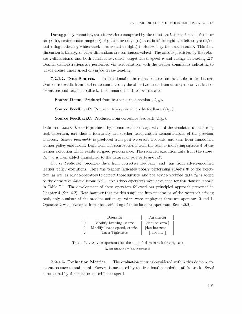
7.2 EMPIRICAL SIMULATION IMPLEMENTATION
During policy execution, the observations computed by the robot are 5-dimensional: left sensorrange (lr), center sensor range (cr), right sensor range (rr), a ratio of the right and left ranges (lr/rr)and a flag indicating which track border (left or right) is observed by the center sensor. This finaldimension is binary; all other dimensions are continuous-valued. The actions predicted by the robotare 2-dimensional and both continuous-valued: target linear speed ν and change in heading ∆θ.Teacher demonstrations are performed via teleoperation, with the teacher commands indicating to(in/de)crease linear speed or (in/de)crease heading.
7.2.1.2. Data Sources. In this domain, three data sources are available to the learner.One source results from teacher demonstrations; the other two result from data synthesis via learnerexecutions and teacher feedback. In summary, the three sources are:
Source Demo: Produced from teacher demonstration (DξD ).
Source FeedbackP: Produced from positive credit feedback (DξP ).
Source FeedbackC: Produced from corrective feedback (DξC ).
Data from Source Demo is produced by human teacher teleoperation of the simulated robot duringtask execution, and thus is identically the teacher teleoperation demonstrations of the previouschapters. Source FeedbackP is produced from positive credit feedback, and thus from unmodifiedlearner policy executions. Data from this source results from the teacher indicating subsets Φ of thelearner execution which exhibited good performance. The recorded execution data from the subsetdΦ ⊆ d is then added unmodified to the dataset of Source FeedbackP.
Source FeedbackC produces data from corrective feedback, and thus from advice-modifiedlearner policy executions. Here the teacher indicates poorly performing subsets Φ of the execu-tion, as well as advice-operators to correct those subsets, and the advice-modified data dΦ is addedto the dataset of Source FeedbackC. Three advice-operators were developed for this domain, shownin Table 7.1. The development of these operators followed our principled approach presented inChapter 4 (Sec. 4.2). Note however that for this simplified implementation of the racetrack drivingtask, only a subset of the baseline action operators were employed; these are operators 0 and 1.Operator 2 was developed from the scaffolding of these baseline operators (Sec. 4.2.2).
Operator Parameter0 Modify heading, static [dec inc zero ]1 Modify linear speed, static [dec inc zero ]2 Turn Tightness [ dec inc ]
Table 7.1. Advice-operators for the simplified racetrack driving task.
[Key: (dec/inc)=(de/in)crease]
7.2.1.3. Evaluation Metrics. The evaluation metrics considered within this domain areexecution success and speed. Success is measured by the fractional completion of the track. Speedis measured by the mean executed linear speed.
105

CHAPTER 7. WEIGHTING DATA AND FEEDBACK SOURCES
The weight update in DWL requires that the system provide rewards for learner executions.Reward in our system is formulated as a simple combination of success and speed. In particular,given fractional task completion `T and average linear speed νT for execution T , the reward receivedby that execution is computed as
r =(`T − ¯)+
(νT − ν
)(7.7)
where ¯ and ν are discounted summations of past success and speed respectively, such that ¯←¯+ β
(`T − ¯) and ν ← ν + β
(νT − ν
)(here β = 0.1);
During learner practice, source selection weights are continually updated as new data is providedfrom various sources. A final source weighting wf and dataset Df are the result. For evaluationpurposes, we derive a variety of policies from Df , defined in Table 7.2. In particular, the DWLpolicy All Learned derives from the full set Df and uses learned source weights wf . To examinethe effect of the learned weighting, policy All Equal also derives from the full set Df but weights allsources equally. To examine data source reliability, policies derived from the data of exclusively onesource, DξD ,DξP , or DξC , are also developed, respectively referred to as the Source Demo, SourceFeedbackP, and Source FeedbackC policies.
Data Weight Policy NameDf wf All LearnedDf equal All Equal
DξD ∈ Df - Source DemoDξP ∈ Df - Source FeedbackPDξC ∈ Df - Source FeedbackC
Table 7.2. Policies developed for the empirical evaluation of DWL.
7.2.2. Results
This section presents empirical results from the DWL implementation. Data sources are demon-strated to be unequally reliable in this domain. The automatic data source weighting under DWL isshown to outperform an equal source weighting scheme, and furthermore to perform as well as thebest contributing expert.
7.2.2.1. Unequal Data Source Reliability. To explore the reliability of each data source,track executions were performed using policies derived exclusively from one source (policies SourceC, Source P and Source C ). The results of these executions are presented in Figure 7.2 (solid bars).The performances of the three sources differ in the measures of both success and speed, confirmingthat in this domain the multiple data sources indeed are not equally reliable.
7.2.2.2. Performance Improvement with Weighting. To examine the effects of datasource weighting, executions were first performed using a policy with equal source weights (policyAll Equal). Figure 7.2 shows that according to the success metric (left plot), the performance ofequal weighting policy (green hashed bar) does match that of the best expert (yellow solid bar). Onthe measure of speed however (right plot), the equal weighting policy underperforms all experts.
106

7.2 EMPIRICAL SIMULATION IMPLEMENTATION
Execution Success Execution Speed
Figure 7.2. Mean percent task completion and translational speed with exclusively onedata source (solid bars) and all sources with different weighting schemes (hashed bars).
By contrast, the policy that used source weights wf learned under the DWL algorithm (policyAll Learned) was able to improve upon the equal weight performance, to the point of outperform-ing two of the three experts on average in execution speed. The average performance over 20 testexecutions with the learned weights wf is shown in Figure 7.2 (white hashed bars). In execu-tion speed, the learned weight policy displays superior performance over the equal weight policy(0.61± 0.03ms vs. 0.31± 0.21ms ). In success, similar behavior is seen, with both giving near perfectperformance. Note that the success of the learned weight policy is more variable, however, indi-cated by a larger standard deviation. This variability is attributed to the increased aggressivenessof the learned weight policy, which gambles occasionally running off the track in exchange for higherexecution speeds.
Beyond improving on the performance of the equal weight policy, the learned weight policyfurthermore begins to approach the performance of the best performing data source. The DWLalgorithm thus is able to combine information from all of the data sources in such a manner as tooutperform or match the performances of most contributing experts, and to approach the perfor-mance of the best expert.
7.2.2.3. Automatically Learned Source Weights. Selection weights are learned itera-tively, throughout practice. Figure 7.3 presents the iterative selection weights as they are learned,across practice runs (solid lines). The learned weights appropriately come to favor Source Feed-backC, which is the best performing expert (Fig. 7.2, yellow bars). For reference, also shown is thefractional number of points from each source within the full set D (dashed lines); this fractionalcomposition changes as practice incorporates new data from various sources. Note that not all
107
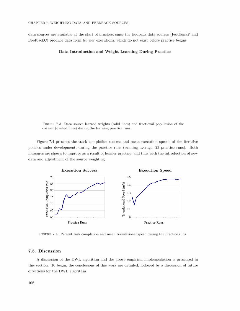
CHAPTER 7. WEIGHTING DATA AND FEEDBACK SOURCES
data sources are available at the start of practice, since the feedback data sources (FeedbackP andFeedbackC) produce data from learner executions, which do not exist before practice begins.
Data Introduction and Weight Learning During Practice
Figure 7.3. Data source learned weights (solid lines) and fractional population of thedataset (dashed lines) during the learning practice runs.
Figure 7.4 presents the track completion success and mean execution speeds of the iterativepolicies under development, during the practice runs (running average, 23 practice runs). Bothmeasures are shown to improve as a result of learner practice, and thus with the introduction of newdata and adjustment of the source weighting.
Execution Success Execution Speed
Figure 7.4. Percent task completion and mean translational speed during the practice runs.
7.3. Discussion
A discussion of the DWL algorithm and the above empirical implementation is presented inthis section. To begin, the conclusions of this work are detailed, followed by a discussion of futuredirections for the DWL algorithm.
108
7.3 DISCUSSION
7.3.1. Conclusions
This section draws together conclusions from this empirical implementation of the DWL algo-rithm. First summarized are aspects of the algorithm that are key to its use as a tool for consideringthe reliability of multiple demonstration and feedback sources. Next a discussion of DWL’s use ofan execution reward is presented.
7.3.1.1. Weighting Data Sources and Feedback Types. The empirical results confirmthat the various data sources are unequally reliable within this domain (Fig. 7.2). Important to re-member is that the learner is not able to choose the source from which it receives data. Furthermore,even a poor data source can be useful, if it is the only source providing data in particular areas ofthe state-space. DWL addresses both of these concerns. Though the learner is not able to choosethe data source, it is able to favor data from certain sources through the DWL weighting scheme.Furthermore, when selecting a data source at prediction time, both this weight and the state-spacesupport of the data source are considered.
Since the expert selection probability formulation of DWL also depends on data support, evena weighting scheme that strongly favors one source will allow for the selection of other sources. Forexample, in Figure 7.3 the learned weights come to strongly favor Source FeedbackC. A source otherthan FeedbackC may be selected in areas of the state-space where FeedbackC has not provideddata, and thus where the dataset associated with Source FeedbackC is lacking in data support.This accounts for the performance differences between policies Source FeedbackC and All Learnedin Figure 7.2. Though the learned weight policy strongly favors selecting the predictions of theSource FeedbackC policy, in areas of the state space unsupported by the data contributed by SourceFeedbackC the algorithm considers the predictions of other sources. Interesting to observe is that inthese experiments, the consideration of the other sources actually degrades performance, suggestingthat even the weakly data-supported predictions of the Source FeedbackC policy are superior to thestrongly-supported predictions of the inferior sources.
This empirical implementation of DWL has furthermore contributed a first evaluation of thepotential variability between the quality of different feedback types. Within this validation domain,feedback types were in fact shown to differ in performance ability. Corrective feedback was foundto be not only the best performing feedback type, but also the best performing data source overall.
7.3.1.2. Reward Formulation and Distribution. The DWL formulation receives a singlereward for an entire execution. Important to underline is that the algorithm does not require a rewardat every execution timestep. The reward therefore only needs to evaluate overall performance, andbe sufficiently rich to learn the data source weights; it is not necessary that the reward be sufficientlyrich to learn the task.
The experimental domain presented here provides reward as a function of performance metricsunrelated to world state. The execution reward, therefore, is not a state reward. In this case, theDWL reward distribution assumes each expert to have contributed to the performance in directproportion to the number of actions they recommended. By contrast, if the execution reward is astate reward, then the reward distribution formulation of DWL assigns equal reward to each state
109

CHAPTER 7. WEIGHTING DATA AND FEEDBACK SOURCES
encountered during the execution. In this case, an alternate approach to reward distribution wouldbe required; ideally one that furthermore considers reward back-propagation to earlier states.
7.3.2. Future Directions
There are many areas for the extension and application of the DWL algorithm. This sectionidentifies a handful of these areas, including alternative approaches to source weighting, a largernumber of more diverse data sources and the further evaluation of different feedback types.
Expert selection probabilities under DWL depend on data support and overall task performance.An interesting extension to the algorithm could further anchor task performance measures to state,and thus consider the varying performance abilities of experts in different areas of the state space.More complex domains and tasks easily could require very different skills in distinct state-spaceareas in order to produce good overall task performance. If demonstration teachers perform well ondistinct subsets of these skills, then anchoring task performance measures to areas of the state spacebecomes particularly relevant.
Most of the data sources in our empirical implementation derived from the data synthesis tech-niques of various feedback types, while only one source derived from actual teacher demonstrations.As discussed in the motivation for this algorithm, multiple teachers contributing demonstrations isa real consideration for LfD policy development. In more complex domains, multiple teachers mayeven be a requirement in order to develop a policy that exhibits good performance, if the full skillset required of the task is not within the capabilities of any single teacher. The inclusion of datafrom multiple teachers with different demonstration styles and skill strengths is thus an interestingfuture application for the DWL algorithm.
This work has contributed a first evaluation of the performance abilities of different feedbacktypes. Just as human demonstrators may vary in their respective abilities to perform certain tasks,so may feedback types be more appropriate for certain domains than for others. Some feedback typesmay be better suited for particular robot platforms or tasks; others may be universally inferior tothe best performing feedback types. Further analysis and evaluation of the performance strengthsand weaknesses of various feedback types is identified as an open area for future research.
7.4. Summary
This chapter has introduced Demonstration Weight Learning (DWL) as an algorithm thatconsiders different types of feedback to be distinct data sources and through a weighting scheme in-corporates demonstration and feedback sources into a policy able to perform a complex task. Datasources are selected through an expert learning inspired paradigm, where each source is treated as anexpert and selection depends on both source weight and data support. Source weights are automat-ically determined and dynamically updated by the algorithm, based on the execution performanceof each expert.
The DWL algorithm was validated within a simulated robot racetrack driving domain. Empiri-cal results confirmed data sources to be unequal in their respective performance abilities of this task.Data source weighting was found to improve policy performance, in the measures of both execution
110

7.4 SUMMARY
success and speed. Furthermore, source weights learned under the DWL paradigm were consistentwith the respective performance abilities of each individual expert.
The differing performance reliabilities between demonstration data sources were discussed, aswell as the subsequent use of a weighting scheme. Future research directions were identified toinclude the development of alternate techniques for weighting data sources. Also identified forfuture research was the application of DWL to complex domains requiring multiple demonstrationteachers with varied skill sets, as well as further investigations that evaluate and compare differentfeedback types.
111


CHAPTER 8
Robot Learning from Demonstration
Learning from Demonstration is a technique that provides a learner with examples of behaviorexecution, from which a policy is derived.1 There are certain aspects of LfD which are common
among all applications to date. One is the fact that a teacher demonstrates execution of a desiredbehavior. Another is that the learner is provided with a set of these demonstrations, and from themderives a policy able to reproduce the demonstrated behavior.
However, the developer still faces many design choices when developing a new LfD system.Some of these decisions, such as the choice of a discrete or continuous action representation, may bedetermined by the domain. Other design choices may be up to the preference of the programmer.These design decisions strongly influence how the learning problem is structured and solved, andwill be highlighted throughout this chapter. To illustrate these design choices, the discussion ofthis chapter is paired with a running pick and place example in which a robot must move a boxfrom a table to a chair. To do so, the object must be 1) picked up, 2) relocated and 3) put down.Alternate representations and/or learning methods for this task will be presented, to illustrate howthese particular choices influence task formalization and learning.
This chapter contributes a framework2 for the categorization of LfD approaches, with a focus onrobotic applications. The intent of our categorization is to highlight differences between approaches.Under our categorization, the LfD learning problem segments into two fundamental phases: gatheringthe examples, and deriving a policy from them. Sections 8.1 and 8.2 respectively describe thesephases. We additionally point the reader to our published survey article, Argall et al. (2009b), thatpresents a more complete categorization of robot LfD approaches into this framework.
1Demonstration-based learning techniques are described by a variety of terms within the published literature, in-cluding Learning by Demonstration (LbD), Learning from Demonstration (LfD), Programming by Demonstration(PbD), Learning by Experienced Demonstrations, Assembly Plan from Observation, Learning by Showing, Learning
by Watching, Learning from Observation, behavioral cloning, imitation and mimicry. While the definitions for someof these terms, such as imitation, have been loosely borrowed from other sciences, the overall use of these terms is
often inconsistent or contradictory across articles. This thesis refers to the general category of algorithms in which a
policy is derived based on demonstrated data as Learning from Demonstration (LfD).2This framework was jointly developed with Sonia Chernova.

CHAPTER 8. ROBOT LEARNING FROM DEMONSTRATION
8.1. Gathering Examples
This section discusses various techniques for executing and recording demonstrations. The LfDdataset is composed of state-action pairs recorded during teacher executions of a desired behavior.Exactly how the examples are recorded, and what the teacher uses as a platform for the execution,varies greatly across approaches. Examples range from sensors on the robot learner recording itsown actions as it is passively teleoperated by the teacher, to a camera recording a human teacheras she executes the behavior with her own body. We formalize the LfD problem statement as inChapter 2 (Sec. 2.1.1.1).
Figure 8.1 introduces our categorization for the various approaches that build a demonstrationdataset, and will be referenced throughout the following subsections. This section begins with apresentation of the design decisions to consider when gathering examples, following by a discussionof potential issues in the transfer of information from the teacher to the learner. The varioustechniques for gathering examples are then detailed.
Figure 8.1. Categorization of approaches to building the demonstration dataset.
8.1.1. Design Decisions
Within the context of gathering teacher demonstrations, we identify two key decisions thatmust be made: the choice of demonstrator, and the choice of demonstration technique. Note thatthese decisions are at times affected by factors such as the complexity of the robot and task. Forexample, teleoperation is rarely used with high degree of freedom humanoids, since their complexmotions are typically difficult to control via joystick.
Most LfD work to date has made use of human demonstrators, although some techniques alsoexamine the use of robotic teachers, hand-written control policies and simulated planners. The choiceof demonstrator further breaks down into the subcategories of (i) who controls the demonstrationand (ii) who executes the demonstration.
For example, consider a robot learning to move a box, as described above. One demonstrationapproach could have a robotic teacher pick up and relocate the box using its own body. In this case
114
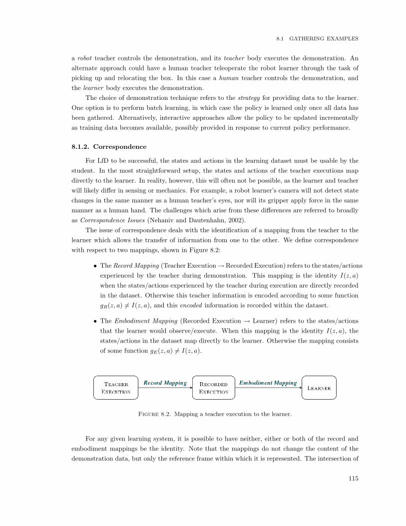
8.1 GATHERING EXAMPLES
a robot teacher controls the demonstration, and its teacher body executes the demonstration. Analternate approach could have a human teacher teleoperate the robot learner through the task ofpicking up and relocating the box. In this case a human teacher controls the demonstration, andthe learner body executes the demonstration.
The choice of demonstration technique refers to the strategy for providing data to the learner.One option is to perform batch learning, in which case the policy is learned only once all data hasbeen gathered. Alternatively, interactive approaches allow the policy to be updated incrementallyas training data becomes available, possibly provided in response to current policy performance.
8.1.2. Correspondence
For LfD to be successful, the states and actions in the learning dataset must be usable by thestudent. In the most straightforward setup, the states and actions of the teacher executions mapdirectly to the learner. In reality, however, this will often not be possible, as the learner and teacherwill likely differ in sensing or mechanics. For example, a robot learner’s camera will not detect statechanges in the same manner as a human teacher’s eyes, nor will its gripper apply force in the samemanner as a human hand. The challenges which arise from these differences are referred to broadlyas Correspondence Issues (Nehaniv and Dautenhahn, 2002).
The issue of correspondence deals with the identification of a mapping from the teacher to thelearner which allows the transfer of information from one to the other. We define correspondencewith respect to two mappings, shown in Figure 8.2:
• The Record Mapping (Teacher Execution→ Recorded Execution) refers to the states/actionsexperienced by the teacher during demonstration. This mapping is the identity I(z, a)when the states/actions experienced by the teacher during execution are directly recordedin the dataset. Otherwise this teacher information is encoded according to some functiongR(z, a) 6= I(z, a), and this encoded information is recorded within the dataset.
• The Embodiment Mapping (Recorded Execution → Learner) refers to the states/actionsthat the learner would observe/execute. When this mapping is the identity I(z, a), thestates/actions in the dataset map directly to the learner. Otherwise the mapping consistsof some function gE(z, a) 6= I(z, a).
Figure 8.2. Mapping a teacher execution to the learner.
For any given learning system, it is possible to have neither, either or both of the record andembodiment mappings be the identity. Note that the mappings do not change the content of thedemonstration data, but only the reference frame within which it is represented. The intersection of
115

CHAPTER 8. ROBOT LEARNING FROM DEMONSTRATION
these configurations is shown in Figure 8.3 and discussed further within subsequent sections. Theleft and right columns represent identity (Demonstration) and non-identity (Imitation) embodimentmappings, respectively. Each column is subdivided by identity (top) or non-identity (bottom) recordmappings. The quadrant contents identify data gathering approaches.
Figure 8.3. Intersection of the record and embodiment mappings.
The embodiment mapping is particularly important when considering real robots, comparedwith simulated agents. Since actual robots execute real actions within a physical environment, pro-viding them with a demonstration involves a physical execution by the teacher. Learning within thissetting depends heavily upon an accurate mapping between the recorded dataset and the learner’sabilities.
Recalling again our box relocation example, consider a human teacher using her own body todemonstrate moving the box, and that the demonstration is recorded by a camera. Let the teacheractions, AT , be represented as human joint angles, and the learner actions, AL, be represented asrobot joint angles. In this context, the teacher’s demonstration of the task is observed by the robotthrough the camera images. The teacher’s exact actions are unknown to the robot; instead, thisinformation must be extracted from the image data. This is an example of a gR(z, a) 6= I(z, a) recordmapping, AT → D. Furthermore, the physical embodiment of the teacher is different from that ofthe robot and his actions (AT ) are therefore not the same as those of the robot (AL). Thereforein order to make the demonstration data meaningful for the robot, a mapping D → AL must beapplied to convert the demonstration into the robot’s frame of reference. This is one example of agE(z, a) 6= I(z, a) embodiment mapping.
Our categorization of LfD data source groups approaches according to the absence or presenceof the record and embodiment mappings. We first split LfD data acquisition approaches into twocategories based on the embodiment mapping, and thus by execution platform:
116

8.1 GATHERING EXAMPLES
• Demonstration: There is no embodiment mapping, because demonstration is performedon the actual robot learner (or a physically identical platform). Thus gE(z, a) ≡ I(z, a).
• Imitation: There exists an embodiment mapping, because demonstration is performed ona platform which is not the robot learner (or a not physically identical platform). ThusgE(z, a) 6= I(z, a).
Approaches are then further distinguished within each of these categories according to record map-ping (Fig. 8.1). We categorize according to these mappings to highlight the levels at which corre-spondence plays a role in demonstration learning. Within a given learning approach, the inclusionof each additional mapping introduces a potential injection point for correspondence difficulties; inshort, the more mappings, the more difficult it is to recognize and reproduce the teacher’s behav-ior. However, mappings also reduce constraints on the teacher and increase the generality of thedemonstration technique.
8.1.3. Demonstration
When teacher executions are demonstrated, by the above definition there exists no embodimentmapping issue between the teacher and learner (left-hand column of Fig. 8.3). There may exist anon-direct record mapping, however, for state and/or actions. This occurs if the states experienced(actions taken) by the demonstrator are not recorded directly, and must instead be inferred fromthe data.
8.1.3.1. Descriptions. Based on this record mapping distinction, we identify two methodsfor providing demonstration data to the robot learner:
• Teleoperation: A demonstration technique in which the robot learner platform is operatedby the teacher, and the robot’s sensors record the execution. The record mapping is direct;thus gR(z, a) ≡ I(z, a).
• Shadowing : A demonstration technique in which the robot learner records the executionusing its own sensors while attempting to match or mimic the teacher motion as theteacher executes the task. The record mapping is not direct; thus gR(z, a) 6= I(z, a).
During teleoperation, a robot is operated by the teacher while recording from its own sensors.Teleoperation provides the most direct method for information transfer within demonstration learn-ing. However, teleoperation requires that operating the robot be manageable, and as a result not allsystems are suitable for this technique. For example low-level motion demonstrations are difficulton systems with complex motor control, such as high degree of freedom humanoids. The strengthof the teleoperation approach is the direct transfer of information from teacher to learner, while itsweakness is the requirement that the robot be operated in order to provide a demonstration.
During shadowing, the robot platform mimics the teacher’s demonstrated motions while record-ing from its own sensors. The states/actions of the true demonstration execution are not recorded;rather, the learner records its own mimicking execution, and so the teacher’s states/actions are in-directly encoded within the dataset. In comparison to teleoperation, shadowing requires an extra
117

CHAPTER 8. ROBOT LEARNING FROM DEMONSTRATION
algorithmic component that enables the robot to track and actively shadow (rather than passivelybe teleoperated by) the teacher. The technique does not, however, require that the teacher be ableto operate the robot in order to provide a demonstration.
Also important to note is that demonstration data recorded by real robots frequently doesnot represent the full observation state of the teacher. This occurs if, while executing, the teacheremploys extra sensors that are not recorded. For example, if the teacher observes parts of the worldthat are inaccessible from the robot’s cameras (e.g. behind the robot, if its cameras are forward-facing), then state, as observed by the teacher, differs from what is actually recorded as data.
8.1.3.2. Implementations. Teleoperation is very effective at reducing the effects of teacher-learner correspondence on the demonstrations, but does require that actively controlling the robotduring the task be manageable, which might not be the case. Shadowing has the advantage of notrequiring the teacher to actively control the robot, but does require that the learner be able to iden-tify and track the teacher; furthermore, the observations made by the teacher during the executionare not directly recorded.
Demonstrations recorded through human teleoperation via a joystick are used in a variety ofapplications, including flying a robotic helicopter (Ng et al., 2004), robot kicking motions (Browninget al., 2004), object grasping (Pook and Ballard, 1993; Sweeney and Grupen, 2007), robotic arm as-sembly tasks (Chen and Zelinsky, 2003) and obstacle avoidance and navigation (Inamura et al., 1999;Smart, 2002). Teleoperation is also applied to a wide variety of simulated domains, ranging fromstatic mazes (Clouse, 1996; Rao et al., 2004) to dynamic driving (Abbeel and Ng, 2004; Chernovaand Veloso, 2008a) and soccer domains (Aler et al., 2005), and many other applications.
Human teachers also employ techniques other than direct joysticking for demonstration. Inkinesthetic teaching, a humanoid robot is not actively controlled but rather its passive joints aremoved through desired motions (Billard et al., 2006). Demonstration may also be performed throughspeech dialog, where the robot is told specifically what actions to execute in various states (Breazealet al., 2006; Lauria et al., 2002; Rybski et al., 2007). Both of these techniques might be viewedas variants on traditional teleoperation, or alternatively as a sort of high level teleoperation. Inplace of a human teacher, hand-written controllers are also used to teleoperate robots (Grollmanand Jenkins, 2008; Rosenstein and Barto, 2004; Smart, 2002).
Demonstrations recorded through shadowing teach navigational tasks by having a robot followan identical-platform robot teacher through a maze (Demiris and Hayes, 2002), follow a humanteacher past sequences of colored markers (Nicolescu and Mataric, 2001a) and mimic routes executedby a human teacher (Nehmzow et al., 2007). Shadowing also has a humanoid learn arm gestures,by mimicking the motions of a human demonstrator (Ogino et al., 2006).
8.1.4. Imitation
For all imitation approaches, as defined above, embodiment mapping issues do exist betweenthe teacher and learner, and so gE(z, a) 6= I(z, a) (right-hand column of Fig. 8.3). There may exista direct or non-direct record mapping, however, for state and/or actions.
118
8.1 GATHERING EXAMPLES
8.1.4.1. Description. Similar to the treatment of demonstration above, approaches forproviding imitation data are further divided by whether the record mapping is the identity or not.
• Sensors on Teacher : An imitation technique in which sensors located on the execut-ing body are used to record the teacher execution. The record mapping is direct; thusgR(z, a) ≡ I(z, a).
• External Observation : An imitation technique in which sensors external to the executingbody are used to record the execution. These sensors may or may not be located on therobot learner. There record mapping is not direct; thus gR(z, a) 6= I(z, a).
The sensors-on-teacher approach utilizes recording sensors located directly on the executingplatform. Having a direct record mapping alleviates one potential source for correspondence dif-ficulties. The strength of this technique is that precise measurements of the example executionare provided. However, the overhead attached to the specialized sensors, such as human-wearablesensor-suits, or customized surroundings, such as rooms outfitted with cameras, is non-trivial andlimits the settings within which this technique is applicable.
Imitation performed through external observation relies on data recorded by sensors locatedexternally to the executing platform. Since the actual states/actions experienced by the teacherduring the execution are not directly recorded, they must be inferred. This introduces a new sourceof uncertainty for the learner. Some LfD implementations first extract the teacher states/actionsfrom this recorded data, and then map the extracted states/actions to the learner. Others mapthe recorded data directly to the learner, without ever explicitly extracting the states/actions ofthe teacher. Compared to the sensors on teacher approach, the data recorded under this techniqueis less precise and less reliable. The method, however, is more general and is not limited by theoverhead of specialized sensors and settings.
8.1.4.2. Implementations. The sensors-on-teacher approach requires specialized sensorsand introduces another level of teacher-learner correspondence, but does not require that the learnerplatform be actively operated or able to track the teacher during task execution. The external-sensors approach has the lowest requirements in terms of specialized sensors or actively operatingthe robot, but does introduce the highest levels of correspondence between the recorded teacherdemonstrations and later executions with the learner platform.
In the sensors-on-teacher approach, human teachers commonly use their own bodies to performexample executions by wearing sensors able to record the human’s state and actions. This is espe-cially true when working with humanoid or anthropomorphic robots, since the body of the robotresembles that of a human. In this case the joint angles and accelerations recorded by a sensor-suitworn by the human during demonstration commonly are used to populate the dataset (Aleotti andCaselli, 2006; Calinon and Billard, 2007; Ijspeert et al., 2002a).
In the external-sensors approach, typically the sensors used to record human teacher executionsare vision-based. Motion capture systems utilizing visual markers are applied to teaching humanmotion (Amit and Mataric, 2002; Billard and Mataric, 2001; Ude et al., 2004) and manipulation tasks(Pollard and Hodgins, 2002). Visual features are tracked in biologically-inspired frameworks that link
119

CHAPTER 8. ROBOT LEARNING FROM DEMONSTRATION
perception to abstract knowledge representation (Chella et al., 2006) and teach an anthropomorphichand to play the game Rock-Paper-Scissors (Infantino et al., 2004).
A number of systems combine external sensors with other information sources; in particular,with sensors located directly on the teacher (Lopes and Santos-Victor, 2005; Lieberman and Breazeal,2004; Mataric, 2002). Other approaches combine speech with visual observation of human gestures(Steil et al., 2004) and object tracking (Demiris and Khadhouri, 2006), within the larger goal ofspeech-supported LfD learning.
Several works also explore learning through the external observation of non-human teachers. Arobot learns a manipulation task through visual observation of an identical robotic teacher (Dillmannet al., 1995), and a simulated agent learns about its own capabilities and unvisited parts of the statespace by observing other simulated agents (Price and Boutilier, 2003). A generic framework forsolving the embodiment correspondence problem has a robotic agent learn new behaviors throughimitation of another, possibly physically different, agent (Alissandrakis et al., 2004).
8.1.5. Other Approaches
Within LfD there do exist exceptions to the data source categorization we have presented here.These exceptions record only states during demonstration, without recording actions. For example,by having a human draw a path through a 2-D representation of the physical world, high levelpath-planning demonstrations are provided to a rugged outdoor robot (Ratliff et al., 2006) and asmall quadruped robot (Ratliff et al., 2007; Kolter et al., 2008). Since actions are not provided inthe dataset, no state-action mapping is learned for action selection. Instead, actions are selected atruntime by employing low level motion planners and controllers (Ratliff et al., 2006, 2007), or byproviding state-action transition models (Kolter et al., 2008).
8.2. Deriving a Policy
This section discusses the various techniques for deriving a policy from a dataset of state-action examples, acquired using one of the above data gathering methods. We identify three coreapproaches within LfD to deriving policies from demonstration data, introduced in the followingsection. Across all approaches, minimal parameter tuning and fast learning times requiring fewtraining examples are desirable.
We identify three core approaches within LfD to deriving a policy. Shown in Figure 8.4, werefer to these approaches as mapping function, system model, and plans:
• Mapping Function: Demonstration data is used to directly approximate the underlyingfunction mapping from the robot’s state observations to actions (f() : Z → A).
• System Model : Demonstration data is used to determine a model of the world dynamics(T (s′|s, a)), and possibly a reward function (R(s)). A policy is then derived using thisinformation.
120
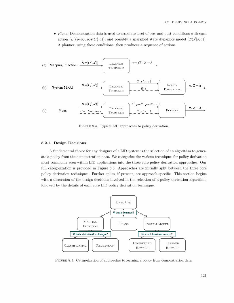
8.2 DERIVING A POLICY
• Plans: Demonstration data is used to associate a set of pre- and post-conditions with eachaction (L({preC, postC}|a)), and possibly a sparsified state dynamics model (T (s′|s, a)).A planner, using these conditions, then produces a sequence of actions.
Figure 8.4. Typical LfD approaches to policy derivation.
8.2.1. Design Decisions
A fundamental choice for any designer of a LfD system is the selection of an algorithm to gener-ate a policy from the demonstration data. We categorize the various techniques for policy derivationmost commonly seen within LfD applications into the three core policy derivation approaches. Ourfull categorization is provided in Figure 8.5. Approaches are initially split between the three corepolicy derivation techniques. Further splits, if present, are approach-specific. This section beginswith a discussion of the design decisions involved in the selection of a policy derivation algorithm,followed by the details of each core LfD policy derivation technique.
Figure 8.5. Categorization of approaches to learning a policy from demonstration data.
121

CHAPTER 8. ROBOT LEARNING FROM DEMONSTRATION
Returning again to our box moving example, suppose a mapping function approach is used toderive the policy. A function f() : Z → A is learned that maps the observed state of the world, forexample the 3-D location of the robot’s end effector, to an action which guides the learner towardsthe goal state, for example the desired end effector motor speed. Consider instead using a systemmodel approach. Here a state transition model T (s′|s, a) is learned, for example that taking the pickup action when in state box on table results in state box held by robot. Using this model, a policy isderived that indicates the best action to take when in a given state, such that the robot is guidedtowards the goal state. Finally, consider using a planning approach. The pre- and post-conditions ofexecuting an action L({preC, postC}|a) are learned from the demonstrations. For example, the pickup action requires the box on table pre-condition, and results in the box held by robot post-condition.A planner uses this learned information to produce a sequence of actions that lead to the goal state.
8.2.2. Problem Space Continuity
When selecting a technique for policy derivation, the continuity of the action representationwithin the demonstration set is a key factor. Action-space continuity is determined both by thetask and robot capabilities, and restricts the applicability of the various derivation approaches.For example, a policy with continuous-valued actions can be derived with regression techniquesand thus under the mapping function approximation approach, but is unlikely to be representedwithin a planning domain where each action must be enumerated and associated with pre- andpost-conditions.
The question of problem-space continuity plays a prominent role within the context of state andaction representation, and many valid representations frequently exist for the same domain. Withinour robot box moving example, one option could be to discretize state, such that the environmentis represented by boolean features such as box on table and box held by robot. Alternatively, acontinuous state representation could be used in which the state is represented by the 3-D positionsof the robot’s end effector and the box. Similar discrete or continuous representations may be chosenfor the robot’s actions. In designing a domain, the continuity of the problem space is influencedby many factors, such as the desired learned behavior, the set of available actions and whether theworld is simulated or real.
We additionally note that LfD can be applied at a variety of action control levels, dependingon the problem formulation. Here roughly grouped into three control levels, LfD has been appliedto: low-level actions for motion control, basic high-level actions (often called action primitives) andcomplex behavioral actions for high-level control. Note that this is a somewhat different considera-tion to action-space continuity. For example, a low-level motion could be formulated as discrete orcontinuous, and so this single action level can map to either continuity space. As a general technique,LfD can be applied at any of these action levels. Most important in the context of policy derivation,however, is whether actions are continuous or discrete, and not their control level.
8.2.3. Mapping Function
The mapping function approach to policy learning calculates a function that approximates thestate to action mapping, f() : Z → A, for the demonstrated behavior (Fig. 8.4a).
122

8.2 DERIVING A POLICY
8.2.3.1. Description. The goal of this type of algorithm is to reproduce the underlyingteacher policy, which is unknown, and to generalize over the set of available training examples suchthat valid solutions are also acquired for similar states that may not have been encountered duringdemonstration.
The details of function approximation are influenced by many factors. These include: whetherthe state input and action output are continuous or discrete; whether the generalization techniqueuses the data to approximate a function prior to execution time or directly at execution time; whetherit is feasible or desirable to keep the entire demonstration dataset around throughout learning, andwhether the algorithm updates online.
In general, mapping approximation techniques fall into two categories depending on whetherthe prediction output of the algorithm is discrete or continuous. Classification techniques are usedto produce discrete output, and regression techniques produce continuous output. Many techniquesfor performing classification and regression have been developed outside of LfD; the reader is referredto Hastie et al. (2001) for a full discussion.
8.2.3.2. Implementations. Mapping function approaches directly approximate the state-action mapping through classification or regression techniques. We begin with a presentation ofclassification applications, followed by regression. Since regression has been the policy derivationtechnique employed in this thesis, it will be presented in greater detail than the other techniques.
Classification approaches categorize their input into discrete classes, thereby grouping similarinput values together. In the context of policy learning, the input to the classifier is robot statesand the discrete output classes are robot actions.
Discrete low-level robot actions include basic commands such as moving forward or turning.Classifiers have been learned for a variety of tasks, including Gaussian Mixture Models (GMMs) forsimulated driving (Chernova and Veloso, 2007), decision trees for simulated airplane flying (Sammutet al., 1992) and Bayesian networks for navigation and obstacle avoidance (Inamura et al., 1999).
Discrete high-level robot actions range from basic motion primitives to high-level robot behav-iors. Motion primitives learned from demonstration include a manipulation task using k -NearestNeighbors (k -NN) (Pook and Ballard, 1993), an assembly task using Hidden Markov Models (HMMs)(Hovland et al., 1996) and a variety of human torso motions using vector-quantization (Mataric,2002). High-level behaviors are generally developed (by hand or learned) prior to task learning, anddemonstration teaches the selection of these behaviors. For example, HMMs classify demonstrationsinto gestures for a box sorting task with a Pioneer robot (Rybski and Voyles, 1999), and the Bayesianlikelihood method is used to select actions for a humanoid robot in a button pressing task (Lockerdand Breazeal, 2004).
Regression approaches map demonstration states to continuous action spaces. Similar to clas-sification, the input to the regressor is robot states, and the continuous output are robot actions.Since the continuous-valued output often results from combining multiple demonstration set actions,typically regression approaches are applied to low-level motions, and not to high-level behaviors. Akey distinction between methods is whether the mapping function approximation occurs at run time,
123

CHAPTER 8. ROBOT LEARNING FROM DEMONSTRATION
or prior to run time. We frame the summary of regression techniques for LfD along a continuumbetween these two extremes.
At one extreme on the regression continuum lies Lazy Learning (Atkeson et al., 1997), wherefunction approximation does not occur until a current observation point in need of mapping ispresent. The simplest Lazy Learning technique is k -NN, which is applied to action selection within arobotic marble-maze domain (Bentivegna, 2004). More complex approaches include Locally WeightedRegression (LWR) (Cleveland and Loader, 1995). One LWR technique further anchors local func-tions to the phase of nonlinear oscillators (Schaal and Sternad, 1998) to produce rhythmic move-ments, specifically drumming (Ijspeert et al., 2002b) and walking (Nakanishi et al., 2004) patternswith a humanoid robot. While Lazy Learning approaches are fast and expend no effort approximat-ing the function in areas which are unvisited during execution time, they do require keeping aroundall of the training data.
In the middle of the regression continuum lie techniques in which the original data is convertedto another, possibly sparsified, representation prior to run time. This converted data is then used byLazy Learning techniques at run time. For example, Receptive Field Weighted Regression (RFWR)(Schaal and Atkeson, 1998) first converts demonstration data to a Gaussian and local linear modelrepresentation. Locally Weighted Projection Regression (LWPR) (Vijayakumar and Schaal, 2000)extends this approach to scale with input data dimensionality and redundancy. Both RFWR andLWPR are able to incrementally update the number of representative Gaussians as well as regressionparameters online. Successful robotics applications using LWPR include an AIBO robot performingbasic soccer skills (Grollman and Jenkins, 2008) and a humanoid playing the game of air hockey(Bentivegna, 2004). The approaches at this position on the continuum benefit from not needing toevaluate all of the training data at run time, but at the cost of extra computation and generalizationprior to execution.
At the opposite extreme on the regression continuum lie approaches which form a completefunction approximation prior to execution time. At run time, they no longer depend on the presenceof the underlying data (or any modified representations thereof). Neural Network (NN) techniquesenable autonomous vehicle driving (Pomerleau, 1991) and peg-in-hole task execution with a robotarm (Dillmann et al., 1995). Also possible are statistical approaches that represent the demonstrationdata in a single or mixture distribution which is sampled at run time, for example a joint distributionfor grasping (Steil et al., 2004), Gaussian Mixture Regression (GMR) for gestures (Calinon andBillard, 2007) and Sparse On-Line Gaussian Processes (SOGP) for soccer skills (Grollman andJenkins, 2008). The regression techniques in this area all have the advantage of no training dataevaluations at run time, but are the most computationally expensive prior to execution. Additionally,some of the techniques, for example NN, can suffer from “forgetting” mappings learned earlier, aproblem of particular importance when updating the policy online.
8.2.4. System Models
The system model approach to LfD policy learning uses a state transition model of the world,T (s′|s, a), and derives a policy π : Z → A from this model (Fig. 8.4b).
124
8.2 DERIVING A POLICY
8.2.4.1. Description. This approach is typically formulated within the structure of Re-inforcement Learning (RL). The transition function T (s′|s, a) generally is defined from the demon-stration data and any additional autonomous exploration the robot may do. To derive a policy fromthis transition model, a reward function R(s), that associates reward value r with world state s,must be either learned from demonstrations or defined by the user.
The goal of RL is to maximize cumulative reward over time. The expected cumulative futurereward of the state under the current policy is represented by further associating each state s with avalue according to the function V (s) (or associating state-action pair s, a with a Q-value accordingto the function Q(s, a)). State values may be represented by the Bellman Equation:
V π(s) =∫a
π(s, a)∫s′T (s′|s, a) [r(s) + γV π(s′)] ds′da (8.1)
where V π(s) is the value of state s under policy π, and γ represents a discounting factor on futurerewards. How to use these values to update a policy, and how to update them effectively online, is asubject of much research outside of LfD. Unlike function approximation techniques, RL approachestypically do not generalize state and demonstrations must be provided for every discrete state. Fora full review of RL, the reader is referred to Sutton and Barto (1998).
Reward is the motivation behind state and action selection, and consequently also guides taskexecution. Defining a reward function to accurately capture the desired task behavior, however, isnot always obvious. Approaches may therefore be categorized according to the source of the rewardfunction. Some approaches engineer the reward function, as seen in classical RL implementations.Other approaches, learn a reward function from the demonstration data.
8.2.4.2. Implementations. Within most applications of the LfD system model approach,RL is employed and the reward function is manually defined by the user. User-defined rewards tendto be sparse, meaning that the reward value is zero except for a few states, such as around obstaclesor near the goal. Various demonstration-based techniques therefore have been defined to aid therobot in locating the rewards and to prevent extensive periods of blind exploration.
Demonstration may be used to highlight interesting areas of the state space in domains withsparse rewards, for example using teleoperation to show the robot the reward states and thus elim-inating long periods of initial exploration in which no reward feedback is acquired (Smart andKaelbling, 2002). Both reward and action demonstrations influence the performance of the learnerin the supervised actor-critic reinforcement learning algorithm (Sutton and Barto, 1998), applied toa basic assembly task using a robotic manipulator (Rosenstein and Barto, 2004).
Defining an effective reward function for real world systems, however, can be a non-trivial issue.One subfield within RL that addresses this is Inverse Reinforcement Learning (Russell, 1998), wherethe reward function is learned rather than hand-defined. Several LfD algorithms examine learninga reward function from demonstration. For example, a reward function is learned by associatinggreater reward with states similar to those encountered during demonstration, and is combined withRL techniques to teach a pendulum swing-up task to a robotic arm (Atkeson and Schaal, 1997).
125

CHAPTER 8. ROBOT LEARNING FROM DEMONSTRATION
Rewarding similarity between teacher demonstrated and robot-executed trajectories is one ap-proach to learning a reward function. Example approaches include a Bayesian model formulation(Ollis et al., 2007), and another that further provides greater reward to positions close to the goal(Guenter and Billard, 2007). Trajectory comparison based on state features guarantees that a cor-rect reward function (Abbeel and Ng, 2004), and furthermore the correct behavior (Ratliff et al.,2006), is learned from feature count estimation. Extensions of this approach decompose the taskdemonstration into hierarchies for a small legged robot (Kolter et al., 2008; Ratliff et al., 2007), andresolve feature count ambiguities (Ziebart et al., 2008). Both a transition function T (s′|s, a) andreward function R(s) are learned for acrobatic helicopter maneuvers (Abbeel et al., 2007).
Finally, real robot applications tend to employ RL in ways not typically seen in the classical RLpolicy derivation algorithms. This is because even in discrete state-action spaces the cost of visitingevery state, and taking every action from each state, becomes prohibitively high and further couldbe physically dangerous. One approach is to use simulation to seed an initial world model, T (s′|s, a),for example using a planner operating on a simulated version of a marble maze robot (Stolle andAtkeson, 2007). The opposite approach derives a model of robot dynamics from demonstrationbut then uses the model in simulation, for example to simulate robot state when employing RL tooptimize a NN controller for autonomous helicopter flight (Bagnell and Schneider, 2001) and invertedhelicopter hovering (Ng et al., 2004). The former implementation additionally pairs the hand-engineered reward with a high penalty for visiting any state not encountered during demonstration,and the latter additionally makes the explicit assumption of a limited class of feasible controllers.
8.2.5. Plans
The plans approach to policy learning views demonstration executions as example plans, anduses the demonstration data to model the conditions of these plans. More specifically, the policy isa plan, and is represented as a sequence of actions that lead from the initial state to the final goalstate (Fig. 8.4c).
8.2.5.1. Description. Plans are typically described in terms of action pre- and post-conditions. An action pre-condition defines the state that must be established before the actionmay be executed. An action post-condition defines the state that results from the action execution.Typically these pre- and post-conditions are learned from the demonstration data. LfD techniquesunder this approach also frequently have the teacher provide information in the form of annotationsor intentions, in addition to the state-action examples. Algorithms differ based on whether this ad-ditional information is provided, as well as how the rules associating action pre- and post-conditionsare learned.
8.2.5.2. Implementations. One of the first papers to learn execution plans based ondemonstration is Kuniyoshi et al. (1994), in which a plan is learned for object manipulation basedon observations of the teacher’s hand movements. Some approaches use spoken dialog both as atechnique to demonstrate task plans, and also to enable the robot to verify unspecified or unsoundparts of a plan through dialog (Lauria et al., 2002; Rybski et al., 2007). Other planning-basedmethods require teacher annotations, for example to encode plan post-conditions (Friedrich and
126
8.3 SUMMARY
Dillmann, 1995), to draw attention to particular elements of the domain (Nicolescu and Mataric,2003), or to encode information about the task goal (Jansen and Belpaeme, 2006; van Lent andLaird, 2001).
8.3. Summary
Learning from Demonstration (LfD) is an approach for deriving a policy from examples ofbehavior executions by a teacher. This chapter has introduced a framework (Argall et al., 2009b)for the categorization of typical robot applications of LfD. In particular, under this framework theimplementation of a LfD learning system is segmented into two core phases: gathering examples,and deriving a policy from the examples. Design considerations when gathering examples includewho controls and executes a demonstration, and how a demonstration is recorded. Each of thesedecisions influence the introduction of teacher-learner correspondence issues into the learning system.When deriving a policy, one of three core approaches is typically taken, termed here as the mappingfunction approximation, system model and plans approaches.
127

CHAPTER 9
Related Work
The problem of learning a mapping between world state and actions lies at the heart of manyrobotics applications. This mapping, or policy, enables a robot to select an action based on
its current world state. The development of policies by hand is often a very challenging problem,and as a result many machine learning techniques have been applied to policy development. In thisthesis, we consider the particular policy learning approach of Learning from Demonstration (LfD).We focus on its application to low-level motion control domains, and techniques that augmenttraditional approaches to address common limitations within LfD.
This chapter presents robot LfD literature relevant to the work of this thesis. In summary, wehave found a lack within the field (i) of techniques that address particular LfD limitations withincontinuous, frequently sampled, action-space domains, (ii) of techniques that provide focused perfor-mance evaluations, (iii) of LfD applications to motion control for a mobile robot (iv) of algorithmsthat build a policy from primitive behaviors while explicitly addressing LfD limitations and (v) ofapproaches that incorporate data from multiple demonstration sources.
In Section 9.1, LfD applications associated with topics central to the focus of this thesis arepresented. Common limitations found within LfD datasets are discussed in Section 9.2. Algorithmsthat explicitly address limitations within LfD, typically the cause of poor policy performance, arethen presented in Section 9.3.
9.1. LfD Topics Central to this Thesis
In this section, we examine LfD applications particularly relevant to the central topics of thisthesis. The topic crucially related to the work of this thesis is whether an algorithm explicitlyaddresses any limitations in the LfD dataset; we reserve discussion of this topic for the followingsections (Secs. 9.2 and 9.3). The remaining central topics, considered here, include (i) learning low-level motion control from demonstration, (ii) learning and using behavior primitives within a LfDframework and (iii) the incorporation of multiple data sources into a LfD policy.
9.1.1. Motion Control
This section discusses LfD applications to low-level motion control tasks. The focus in thissection is on applications where the actual motion is learned from demonstration; applications that

CHAPTER 9. RELATED WORK
learn from demonstration some other aspect of a motion task, for example how to select betweenhand-coded motion primitives, are not discussed here. We segment approaches into three motorstrata: motor poses, motions for a stationary robot and motions for a mobile robot.
We define motor poses as stationary configurations of the robot, that are formed throughmotion. While the motion is learned from demonstration, it merely enables the target behavior. Forexample, through demonstration an anthropomorphic hand learns the hand formations and rulesfor the game Rock-Paper-Scissors (Infantino et al., 2004). Using GMR, a humanoid robot is taughtbasketball referee signals by pairing kinesthetic teachings with human teacher executions recordedvia wearable motion sensors (Calinon and Billard, 2007).
The most common application of LfD to motion control is for motion tasks on a stationaryrobot. Early work by Atkeson and Schaal (1997) has a robotic arm learn pole balancing via stereo-vision and human demonstration. The recorded joint angles of a human teach drumming patternsto a 30-DoF humanoid (Ijspeert et al., 2002a). Motion capture systems utilizing visual markers areapplied to teaching human arm motion (Amit and Mataric, 2002; Ude et al., 2004) and manipulationtasks (Pollard and Hodgins, 2002). The combination of 3D marker data with torso movement andjoint angle data is used for applications on a variety of simulated and robot humanoid platforms(Mataric, 2002). A human wearing sensors controls a simulated human, which maps to a simulatedrobot and then to a real robot arm (Aleotti and Caselli, 2006). A force-sensing glove is combined withvision-based motion tracking to teach grasping movements (Lopes and Santos-Victor, 2005; Voylesand Khosla, 2001). Generalized dexterous motor skills are taught to a humanoid robot (Liebermanand Breazeal, 2004), and demonstration teaches a humanoid to grasp novel and known householdobjects (Steil et al., 2004).
For demonstrated motion control on a mobile robot, a seminal work by Pomerleau (1991) useda Neural Network to enable autonomous driving of a van at speed on a variety of road types.Demonstrations contribute to the development of a controller for a robotic helicopter flight, invertedhovering and acrobatic maneuvers (Abbeel et al., 2007; Bagnell and Schneider, 2001; Ng et al., 2004).An AIBO robot is taught basic soccer skills (Grollman and Jenkins, 2008), recorded joint anglesteach a humanoid walking patterns within simulation (Nakanishi et al., 2004) and a wheeled robotlearns obstacle avoidance and corridor following (Smart, 2002).
9.1.2. Behavior Primitives
To build a policy from multiple smaller policies, or behavior primitives, is an interesting de-velopment technique to combine with LfD. This technique is attractive for a variety of reasons,including a natural framework for scaling up existing behaviors to more complex tasks and domains,and the potential for primitive reuse within other policies.
Pook and Ballard (1993) classify primitive membership using k -NN, and then recognize eachprimitive within the larger demonstrated task via Hidden Markov Models (HMMs), to teach a robotichand and arm an egg flipping manipulation task. Demonstrated tasks are decomposed into a libraryof primitives for a robotic marble maze (Stolle and Atkeson, 2007), and behavior primitives aredemonstrated and then combined by the human teacher into a larger behavior (Saunders et al.,2006). The use of hand-coded behavior primitives to build larger tasks learned from demonstration
130

9.2 LIMITATIONS OF THE DEMONSTRATION DATASET
include a humanoid playing the game of air-hockey (Bentivegna, 2004) and a Pioneer performingnavigation tasks (Nicolescu and Mataric, 2003).
A biologically-inspired framework is presented in Mataric (2002), which automatically ex-tracts primitives from demonstration data, classifies data via vector-quantization and then composesand/or sequences primitives within a hierarchical NN. The work is applied to a variety of test beds,including a 20 DoF simulated humanoid torso, a 37 DoF avatar (a simulated humanoid which re-sponds to external sensors), Sony AIBO dogs and small differential drive Pioneer robots. Underthis framework, the simulated humanoid torso is taught a variety of dance, aerobics and athleticsmotions (Jenkins et al., 2000), the avatar reaching patterns (Billard and Mataric, 2001) and thePioneer sequenced location visiting tasks (Nicolescu and Mataric, 2001b).
9.1.3. Multiple Demonstration Sources and Reliability
The incorporation of data from multiple demonstration sources is a topic that has receivedlimited attention from the LfD community. Furthermore, assessing the reliability between differentdemonstration sources has not been explicitly addressed in the literature. A closely related topic,however, is the assessment of the worth and reliability of datapoints within the demonstration set.
Multiple demonstration teachers are employed for the purposes of isolating salient character-istics of the task execution (Pook and Ballard, 1993). Demonstration information is also solicitedfrom multiple other agents to speed up learning (Oliveira and Nunes, 2004). Multiple sources ofdemonstration data on the whole, however, remains largely unaddressed.
Data worth is addressed by actively removing unnecessary or inefficient elements from a teacherdemonstration (Kaiser et al., 1995). The reliability of a dataset in different areas of the state-spaceis assessed through the use of a confidence measure to identify undemonstrated or ambiguouslydemonstrated areas of the state-space (Chernova and Veloso, 2007; Grollman and Jenkins, 2007).
9.2. Limitations of the Demonstration Dataset
LfD systems are inherently linked to the information provided in the demonstration dataset.As a result, learner performance is heavily limited by the quality of this information. One commoncause for poor learner performance is due to dataset sparsity, or the existence of areas of the statespace that have not been demonstrated. A second cause is poor quality of the dataset examples,which can result from a teacher’s inability to perform the task optimally or poor correspondencebetween the teacher and learner.
9.2.1. Undemonstrated State
All LfD policies are limited by the availability of training data because, in all but the most simpledomains, the teacher is unable to demonstrate the correct action from every possible state. Thisraises the question of how the robot should act when it encounters a state for which no demonstrationhas been provided. Here existing methods for dealing with undemonstrated state are categorized intotwo approaches: generalization from existing demonstrations, and acquisition of new demonstrations.
131
CHAPTER 9. RELATED WORK
9.2.1.1. Generalization from Existing Demonstrations. Here techniques that useexisting data to deal with undemonstrated state are presented as used within each of the core policyderivation approaches.
Within the function mapping approach, undemonstrated state is dealt with through state gen-eralization. Generalizing across inputs is a feature inherent to robust function approximation. Theexact nature of this generalization depends upon the specific classification or regression techniqueused. Some examples are approaches that range from strict grouping with the nearest dataset pointstate, as in 1-Nearest Neighbor, to soft averaging across multiple states, as in kernelized regression.
Within the system model approach, undemonstrated state can be addressed through stateexploration. State exploration is often accomplished by providing the learner with an explorationpolicy that guides action selection within undemonstrated states. Based on rewards provided bythe world, the performances of these actions are automatically evaluated. This motivates the issueof Exploration vs. Exploitation; that is, of determining how frequently to take exploratory actionsversus following the set policy. Note that taking exploratory steps on a real robot system is oftenunwise, for safety and stability reasons.
9.2.1.2. Acquisition of New Demonstrations. A fundamentally different approach todealing with undemonstrated state is to acquire additional demonstrations when novel states areencountered by the robot. Note that such an approach is not equivalent to providing all of thesedemonstrations prior to learner execution, as that requires the teacher to know beforehand everystate the learner might encounter during execution, a generally impossible expectation in real worlddomains. One set of techniques has the teacher decide when to provide new examples, based onlearner performance. Another set has the learner re-engage the teacher to request additional demon-strations. Under such a paradigm, the responsibility of selecting states for demonstration now isshared between the robot and teacher; see Section 9.3.1 for further details.
9.2.2. Poor Quality Data
The quality of a learned LfD policy depends heavily on the quality of the provided demonstra-tions. In general, approaches assume the dataset to contain high quality demonstrations performedby an expert. In reality, however, teacher demonstrations may be ambiguous, unsuccessful or sub-optimal in certain areas of the state space.
9.2.2.1. Suboptimal or Ambiguous Demonstrations. Inefficient demonstrations maybe dealt with by eliminating parts of the teacher’s execution that are suboptimal. Suboptimality ismost common in demonstrations of low-level tasks, for example movement trajectories for roboticarms. In these domains, demonstrations serve as guidance instead of offering a complete solution.Other approaches smooth or generalize over suboptimal demonstrations in such a way as to improveupon the teacher’s performance. Further details are provided in Section 9.3.4.
Dataset ambiguity may be caused by uncaptured elements of the record mapping. Additionally,dataset ambiguity may be caused by teacher demonstrations that are inconsistent between multipleexecutions. This type of ambiguity can arise due to the presence of multiple equally applicableactions, and the result is that a single state maps to different actions. In the case of discrete actions,
132

9.3 ADDRESSING DATASET LIMITATIONS
this results in inconsistent learner behavior. In the case of continuous actions, depending on theregression technique, this can result in an averaged behavior that is dangerously dissimilar to eitherdemonstrated action.
9.2.2.2. Learning from Experience. An altogether different approach to dealing withpoor quality data is for the student to learn from experience. If the learner is provided with feedbackthat evaluates its performance, this may be used to update its policy. This evaluation is generallyprovided via teacher feedback, or through a reward as in RL.
Learning from experience under the mapping function approximation approach is relativelyuncommon. If present, however, performance evaluations can be used to modify the state-actionmapping function. This occurs either by modifying the contents of the dataset, or modifying themanner of function approximation. Performance evaluations are generally provided automaticallyby the world or through teacher feedback. Beyond providing just an evaluation of performance,a human teacher may also provide a correction on the executed behavior. For the most part,approaches that employ teacher corrections do so within discrete-action domains; further details areprovided in Section 9.3.3.
Most use of RL-type rewards occurs under the system model approach. To emphasize, theseare rewards seen during learner execution with its policy, and not during teacher demonstrationexecutions. State rewards are typically used to update state values V (s) (or Q-values Q(s, a)).Within a system model LfD formulation, student execution information may also be used to updatea learned dynamics model T (s′|s, a). For further details, see Section 9.3.3.
Important to underline is the advantage of providing demonstrations and employing LfD beforeusing traditional policy learning from experience techniques. Many traditional learning approaches,such as exploration-based methods like RL, are not immediately applicable to robots. This is duelargely to the constraints of gathering experience on a real system. To physically execute all actionsfrom every state will likely be infeasible, may be dangerous, and will not scale with continuous statespaces. However, the use of these techniques to evaluate and improve upon the experiences gainedthrough an LfD system has proven very successful.
9.3. Addressing Dataset Limitations
The quality of a policy learned from demonstration is tightly linked to the quality of thedemonstration dataset. Many LfD learning systems therefore have been augmented to enable learnerperformance to improve beyond what was provided in the demonstration dataset. One techniquefor addressing dataset limitations, discussed in Section 9.3.1, is to provide the learner with moreteacher demonstrations. The intent here is to populate undemonstrated state-space areas, or toclarify ambiguous executions.
There are LfD limitations, however, that are not able to be addressed through demonstration,for example poor teacher-to-learner correspondence or suboptimal teacher ability. Learning fromexperience is one approach for addressing poor policy performance that does not depend on teacherdemonstration. Approaches that extend LfD to have the robot update its policy based on itsexecution experience are presented in Sections 9.3.2 and 9.3.3. We note that learning from experience
133
CHAPTER 9. RELATED WORK
is a rich research area outside of the realm of LfD and a variety of techniques exist, the most popularof which is RL. We focus this presentation, however, to applications of experience learning techniqueswithin LfD particularly.
9.3.1. More Demonstrations
Providing the learner with more teacher demonstrations can address the limitation of undemon-strated or ambiguously demonstrated areas of the state-space. This technique is most popularamongst approaches that derive policies by approximating the underlying state→action mappingfunction. Note that under the mapping function approach, to a certain extent the issue of undemon-strated state is already addressed through the state generalization of the classification or regressionpolicy derivation techniques. State generalization is automatically performed by the statistical tech-niques used to derive the policy, ranging from the simplest which group unseen states to the nearestdataset state (e.g. k-NN ) to more complex approaches such as state mixing. In undemonstratedstate-space areas, however, this generalization may not be correct.
One set of approaches acquire new demonstrations by enabling the learner to evaluate itsconfidence in selecting a particular action, based on the confidence of the underlying classificationalgorithm. In Chernova and Veloso (2007, 2008a) the robot requests additional demonstration instates that are either very different from previously demonstrated states or in states for which asingle action can not be selected with certainty. In Grollman and Jenkins (2007) the robot indicatesto the teacher its certainty in performing various elements of the task, and the teacher may choose toprovide additional demonstrations indicating the correct behavior to perform. More demonstrationis provided through kinesthetic teaching, where passive humanoid joints are moved by the teacherthrough the desired motions, at the teacher’s discretion in Calinon and Billard (2007).
9.3.2. Rewarding Executions
Providing the learner with an evaluation of policy performance is another approach to addressingdataset limitations. By incorporating this evaluation into a policy update, performance may improve.
Policy evaluations are most commonly provided through state rewards. This technique is there-fore popular amongst policies formulated under the system model approach, which are typically de-rived using RL techniques. Note that under this policy derivation formulation, state generalizationdoes not occur. Since the goal of RL is to maximize cumulative reward over time, by updating thestate values with rewards received, a policy derived under this paradigm also updates. We emphasizethat these are rewards seen during learner execution with its policy, and not during teacher demon-stration executions. Note that reward functions tend to be sparse and thus credit performance onlyin key states, such as those near a goal or a point of failure. Earlier performance that leads to poorperformance is therefore not always credited.
Smart (2002) seeds the robot’s reward and transition functions with a small number of subopti-mal demonstrations, and then optimizes the policy through exploration and RL. A similar approachis taken by Peters and Schaal (2008) in their use of the Natural Actor Critic algorithm, a variant ofRL, to learn a motor primitives for a 7-DoF robotic arm. In Stolle and Atkeson (2007), the worldmodel is seeded with trajectories produced by a planner operating on a simulated version of their
134

9.3 ADDRESSING DATASET LIMITATIONS
robot, and learner execution results in state values being updated. In addition to updating state val-ues, student execution information may be used to update a learned dynamics model T (s′|s, a). Thisapproach is taken by Abbeel and Ng (2005), who seed their world model with teacher demonstra-tions. Policy updates then consist of rederiving the world dynamics after adding learner executionswith this policy (and later updated policies) to the demonstration set.
In Bentivegna (2004), a policy derived under the mapping function approximation approachis updated using RL techniques. The function approximation takes into consideration Q-valuesassociated with paired query-demonstration points, and these Q-values are updated based on learnerexecutions and a developer-defined reward function. Another atypical use of reward is the work ofJansen and Belpaeme (2006), where a student uses binary policy evaluations from a human teacherto prune the set of inferred goals that it maintains within a planning framework.
9.3.3. Correcting Executions
An additional approach to addressing LfD limitations is to directly correct poor predictionsmade during a policy execution. Policy corrections formulated in this manner do not depend onteacher demonstrations. Furthermore, correcting poor predictions provides more focused and de-tailed improvement information than overall performance evaluations or state rewards.
Policy correction has seen limited attention within LfD however. The selection of a policycorrection is sufficiently complex to preclude it being provided with a simple sparse function, asin the case of most state rewards. Approaches that do correct policy predictions therefore providecorrections through human teachers. Furthermore, since the correction likely indicates a preferredstate or action, within the existing literature corrections are only provided within action spaceswhere the actions are discrete and of significant time duration, and therefore sampled relativelyinfrequently. The correct action from a discrete set is provided by a human teacher in Nicolescuand Mataric (2003), and this information updates the structure of a hierarchical Neural Networkof robot behaviors. Discrete action corrections from a human teacher update an action classifier inChernova and Veloso (2008b).
9.3.4. Other Approaches
There are other techniques that address LfD limitations but do not fall within any of the broadertechnique categories already discussed. We first present approaches that consider suboptimal orambiguous demonstrations, followed by those that explore undemonstrated state-space areas.
Suboptimal demonstrations are addressed in Kaiser et al. (1995), who present a method foractively identifying and removing elements of the demonstration that are unnecessary or inefficient,by removing actions that do not contribute to the solution to the task. Other approaches smooth orgeneralize over suboptimal demonstrations in such a way as to improve upon the teacher’s perfor-mance. For example, when learning motion control, data from multiple repeated demonstrations isused to obtain a smoothed optimal path (Aleotti and Caselli, 2006; Delson and West, 1996; Yeasinand Chaudhuri, 2000), and data from multiple teachers encourages more robust generalization (Pookand Ballard, 1993).
135

CHAPTER 9. RELATED WORK
Ambiguous demonstrations are addressed in Friedrich and Dillmann (1995), where the teacherspecifies the level of generality that was implied by a demonstration, by answering the learner’s ques-tions. Other approaches focus on the development of generalized plans with flexible action order (vanLent and Laird, 2001; Nicolescu and Mataric, 2003). Differences in teacher and learner perspectivesduring externally recorded demonstrations are accounted for by having the robot maintain separatebelief estimates for itself and the human demonstrator (Breazeal et al., 2006). Teacher demon-strations that are inconsistent between multiple executions may be handled by modeling equivalentactions choices explicitly in the robot policy (Chernova and Veloso, 2008b).
To visit and evaluate new states not seen in the demonstration set, an exploration policy may beemployed, though we note that taking exploratory steps on a real robot can be inefficient and evendangerous. Executing with an exploration policy may provide information about the world dynamics,and additionally the value of state-action pairs if it is coupled within an approach that evaluatespolicy performance, for example RL. A safe exploration policy is employed by Smart (2002) for thepurposes of gathering robot demonstration data, both to seed and then update a state transitionmodel and reward function. To guide exploration within this work, initially a suboptimal controlleris provided, and once a policy is learned small amounts of Gaussian noise are randomly added tothe greedy actions of this policy. Execution experience also updates a learned transition functionwithout taking explicit exploration steps (Abbeel and Ng, 2005).
9.4. Summary
In summary, Learning from Demonstration is an effective policy development approach thathas been validated on a variety of robotic applications. Algorithms that use demonstration to teachlow level motion control tasks for mobile robots are less common, but do exist.
Given that there are limitations within the LfD paradigm, approaches that provide techniques toimprove beyond the demonstration dataset are noted to be particularly valuable. Popular techniqueseither provide more demonstration data or state rewards. More demonstration, however, is not ableto address all sources of LfD limitations and requires revisiting states, while state rewards are oftenunable to credit early performance that leads to later poor performance and furthermore give noindication of the preferred policy behavior. In this thesis, we identify techniques that address theseadditional causes of LfD limitations, and provide more focused informative performance information,to be especially useful.
In particular, the approach of correcting policy predictions is identified to be a promisingtechnique that does address both of these concerns. Challenges to providing policy corrections,however, have prevented its inclusion the majority of LfD applications that address dataset limi-tations. Furthermore, approaches that correct policies within continuous action-spaces sampled athigh frequency are entirely absent from the literature. These considerations have prompted ourdevelopment of multiple feedback forms, in particular of our corrective advice-operator technique,as well as our F3MRP feedback framework that is suitable for rapidly sampled policy domains.
We also identify techniques that build and incorporate primitive policies within LfD frameworksto be useful, given the potential for policy reuse. Only one existing approach however (Bentivegna,2004) combines a primitive policy framework with techniques that also address dataset limitations.
136

9.4 SUMMARY
Additionally, the incorporation of data from multiple sources is identified as an interesting andrelevant area that has received limited attention within the current LfD literature. Algorithmscontributed in this thesis, FPS and DWL respectively, address each of these topics.
137


CHAPTER 10
Conclusions
This thesis has contributed techniques for the development of motion control algorithms for mobilerobots. Our introduced approaches use human teacher feedback to build and refine policies
learned from demonstration. The most distinguishing characteristics of our feedback techniquesare the capability of providing policy corrections within continuous state-action domains, withoutneeding to revisit the state being corrected, and to provide feedback on multiple execution pointsat once. With these characteristics, our techniques are appropriate for the improvement of low-level motion control policies executed by mobile robots. We use feedback to refine policies learnedfrom demonstration, as well as to build new policies able to accomplish complex motion tasks.In particular, our scaffolding technique allows for the building of complex behaviors from simplermotions learned from demonstration.
Algorithms were introduced that use feedback to build and refine motion control policies formobile robots. In particular, the algorithms Binary Critiquing and Advice-Operator Policy Improve-ment used binary performance flags and corrective advice as feedback, respectively, to refine motioncontrol policies learned from demonstration. The algorithm Feedback for Policy Scaffolding usedmultiple types of feedback to refine primitive motion policies learned from demonstration, and toscaffold them into complex behaviors. The algorithm Demonstration Weight Learning treated dif-ferent feedback types as distinct data sources, and through a performance-based weighting schemecombined data sources into a single policy able to accomplish a complex task.
A variety of techniques were developed to enable the transfer of teacher evaluations of learnerexecution performance into policy updates. Of particular note is the advice-operator formulation,which was a mechanism for correcting motion control policies that exist in continuous action spaces.The Focused Feedback for Mobile Robot Policies framework furthermore enabled the transfer ofteacher feedback to the learner for policies that are sampled at a high frequency.
All contributed feedback mechanisms and algorithms were validated empirically, either on aSegway RMP robot or within simulated motion control domains. In depth discussions of the con-clusions drawn from each algorithm implementation, and the identification of directions for futureresearch, were presented throughout the document in each respective algorithm chapter. In thefollowing sections, the contributions of this thesis are highlighted and summarized.
CHAPTER 10. CONCLUSIONS
10.1. Feedback Techniques
The cornerstone of this thesis is the use of teacher feedback to build and refine motion controlpolicies for mobile robots. Towards this end, multiple feedback forms were developed and employedin this work. The most noteworthy of these was the advice-operator formulation, that allowed for thecorrection of low-level motion control policies. A framework was also contributed, Focused Feedbackfor Mobile Robot Policies, through which feedback was provided on motion control executions andincorporated into policy updates. The combination of these techniques enabled the correction ofpolicies within (i) continuous state-action spaces and (ii) with actions of short duration. Both ofthese topics were previously unaddressed within the LfD literature.
10.1.1. Focused Feedback for Mobile Robot Policies
With the Focused Feedback for Mobile Robot Policies (F3MRP) framework, we contributed atechnique that enables feedback from a teacher to be provided to the learner and incorporated into apolicy update. Key is the application of a single piece of feedback to multiple execution points, whichis necessary for providing focused feedback within rapidly sampled policy domains. In such domainsbehavior spans over multiple execution points, and so to select each point individually would betedious and inefficient. The application of feedback to multiple points is accomplished through avisual display of the mobile robot execution ground path and a segment selection technique.
To associate feedback with the execution, the teacher selects segments of a graphically repre-sented execution trace. The feedback interface provides the human teacher with an indication ofdataset support, which the teacher uses when selecting execution segments to receive good perfor-mance flags. In this work, a discussion of the details involved in developing a feedback framework wasalso provided. Key design decisions were identified as: the type of feedback provided, the feedbackinterface and the manner of feedback incorporation into the policy.
10.1.2. Advice-Operators
Advice-operators were contributed as a mechanism for correcting low-level motion control poli-cies. Paired with the segment selection technique of the F3MRP framework, the advice-operatorformulation allows a single piece of advice to provide continuous-valued corrections on multipleexecution points. Advice-operators are thus appropriate for correcting continuous-valued actionssampled at high frequency, as in low-level motion control domains.
Advice-operators function as mathematical computations on data points that result from alearner execution. They synthesize new advice-modified data points, which are added to the demon-stration dataset and consequently update a policy derived from this set. There are many key advan-tages to using advice to correct a policy. One advantage is that a state does not need to be revisitedto receive a correction, which is particularly useful when revisiting states would involve executingphysical actions on a mobile robot. Another advantage is that actions produced by advice-operatorsare not restricted to those already present in the dataset, and thus are not limited by suboptimalteacher performance or poor teacher-to-learner correspondence.
The success of the advice-operator technique depends on the definition of effective operators.To this end, we furthermore have contributed a principled approach for the development of action
140

10.2 ALGORITHMS AND EMPIRICAL RESULTS
advice-operators. Under this paradigm, a baseline set of operators are automatically defined fromthe available robot actions. A developer may then build new operators, by composing and sequencingexisting operators, starting with the baseline set. The new data points produced from advice areadditionally constrained by parameters automatically set based on the robot dynamics, to firmlyground the synthesized data on a real execution and the physical limits of the robot. Directions forfuture work with advice-operators were identified, and included their application to more complexaction spaces and the further development of observation-modifying operators.
10.2. Algorithms and Empirical Results
This thesis contributed multiple algorithms that build motion control policies for mobile robotsthrough a combination of demonstration and teacher feedback. Each algorithm was empiricallyvalidated, either on a Segway RMP robot or within a simulated motion control domain. A summaryof these algorithms, and their empirical results, are presented here.
10.2.1. Binary Critiquing
The Binary Critiquing (BC) algorithm provided an approach for crediting policy performancewith teacher feedback in the form of negative performance flags. The algorithm was implementedwithin a simulated robot motion interception domain. Empirical results showed improvements insuccess and efficiency as a consequence of the negative credit feedback. Interestingly, the performanceof the final learned policy exceeded the performance of the demonstration policy, without modifyingthe contents of the demonstration dataset. Instead, teacher feedback modified the use of the existingdemonstration data by the regression techniques employed for policy derivation.
This work also provided a discussion of the benefits of using a human for credit assignment.In particular, the human selected portions of an execution to flag as poorly performing. Ratherthan just crediting poor performance where it occurs, segment selection allows for behaviors thatlead to poor performance to receive poor credit as well. Future directions for the BC algorithmincluded directional critiques that consider query point orientation and real-valued critiques thatimpart a measure of relative, rather than just binary, performance. Feedback that is corrective wasalso identified as a potential improvement, motivating the development of advice-operators.
10.2.2. Advice-Operator Policy Improvement
With the Advice-Operator Policy Improvement (A-OPI) algorithm, an approach was providedthat improves policy performance through corrective teacher feedback. A noteworthy contributionof this work is that corrections were efficiently offered in continuous state-action domains sampledat high frequency, through the use of advice-operators.
The algorithm was implemented on a Segway RMP robot performing planar motion tasks. Theinitial case study implementation used a simple set of advice-operators to correct a spatial trajectoryfollowing task. Empirical results showed improvements in precision and efficiency, and both beyondthe abilities of demonstrator. Corrective advice was also found to enable the emergence of novelbehavior characteristics, absent from the demonstration set. The full task implementation useda complex set of advice-operators to correct a more difficult spatial positioning task. Empirical
141

CHAPTER 10. CONCLUSIONS
results showed performance improvement, measured by success and accuracy. Furthermore, theA-OPI policies displayed similar or superior performance when compared to a policy developedfrom exclusively more teleoperation demonstrations. The A-OPI approach also produced noticeablysmaller datasets, without a sacrifice in policy performance, suggesting that the datasets were morefocused and contained smaller amounts of redundant data.
Also presented was discussion of the features of the A-OPI approach that facilitate providingcorrections within low-level motion control domains. In particular, the segment selection techniqueallows multiple actions to be corrected by a single piece of advice. The advice-operator mechanismtranslates high-level advice into continuous-valued corrections. Selection of an operator is reasonablefor a human to perform, since the set of advice-operators is discrete; by contrast, selection from aninfinite set of continuous-valued corrections would not be reasonable. Future directions for the A-OPI algorithm were identified to include interleaving the policy improvement techniques of correctiveadvice and more demonstrations, as well as additional advice formulations.
10.2.3. Feedback for Policy Scaffolding
The Feedback for Policy Scaffolding (FPS) algorithm contributed an approach that uses feed-back to build complex policy behaviors. More specifically, the algorithm operates in two phases. Thefirst phase develops primitive motion behaviors from demonstration and feedback provided throughthe F3MRP framework. The second phase scaffolds these primitive behaviors into a policy ableto perform a more complex task. F3MRP feedback is again employed, in this case to assist thescaffolding and thus enable the development of a sophisticated motion behavior.
The FPS algorithm was implemented within a simulated motion domain that tasked a differen-tial drive robot with driving a racetrack. Primitive behavior policies, which represent simple motioncomponents of this task, were successfully learned through demonstration and teacher feedback.A policy able to drive the full track also was successfully developed, from the primitive behaviorsand teacher feedback. In both phases, empirical results showed policy performance to improve withteacher feedback. Furthermore, all FPS policies outperformed the comparative policies developedfrom teacher demonstration alone. While these exclusively demonstrated policies were able to pro-duce the primitive behaviors, albeit less successfully than the FPS policies, they were not able toperform the more complex task behavior.
Within this work we also discussed the advantages of reusing primitive policies learned fromdemonstration. The benefit of not needing to revisit states to provide corrections was also high-lighted, as the correction techniques of the F3MRP framework were much more efficient than demon-stration at developing the desired robot behaviors. Directions for future research were identified asalternate ways to select between and scaffold primitive behavior policies, other approaches for feed-back incorporation into the complex policy and the validation of this algorithm within a real worldrobot domain.
142

10.3 CONTRIBUTIONS
10.2.4. Demonstration Weight Learning
With the Demonstration Weight Learning (DWL) algorithm, an approach was introduced thattreats different types of feedback as distinct data sources and, through a weighting scheme, incor-porates them into a policy able to perform a complex task. Data sources are selected through anexpert learning-inspired paradigm, and their weights automatically determined based on executionperformance. This paradigm thus allows for the evaluation of multiple feedback sources, and fur-thermore of various feedback types. An additional motivation for this algorithm was our expectationof multiple demonstration teachers within real world applications of LfD.
The DWL algorithm was implemented within a simulated racetrack driving domain. Empiricalresults confirmed an unequal reliability between data sources, and source weighting was found toimprove policy performance. Furthermore, the source weights learned under the DWL paradigmwere consistent with the respective performance abilities of each individual expert. A discussionof the differing reliability and weighting of data sources was presented. Future research directionsidentified were the development of alternate techniques for weighting data sources, the applicationof DWL to complex domains requiring multiple demonstration teachers with diverse skill sets andfurther analysis of the performance variability between different feedback types.
10.3. Contributions
The aim of this thesis was to address two research questions. The first question, How mightteacher feedback be used to address and correct common Learning from Demonstration limitationsin low-level motion control policies?, has been addressed through the following contributions:
• The introduction of the Focused Feedback for Mobile Robot Policies framework as a mech-anism for providing focused feedback on multiple points resulting from policy executionon a mobile robot.
• The development of advice-operators as a technique for providing corrections within con-tinuous state-action spaces, in addition to the development of other novel feedback forms.
• The introduction of the Binary Critiquing and Advice-Operator Policy Improvement al-gorithms, that refine motion control policies learned from demonstration through the in-corporation these novel feedback forms and use of our contributed feedback framework.
The second question, In what ways might the resulting feedback techniques be incorporated into morecomplex policy behaviors? has been addressed by these contributions:
• The introduction of the Feedback for Policy Scaffolding algorithm, that uses multiplefeedback types both to refine motion behavior primitives learned from demonstration, andto scaffold them into a policy able to accomplish a more complex behavior.
143

CHAPTER 10. CONCLUSIONS
• The introduction of the Demonstration Weight Learning algorithm, that combines multipledemonstration and feedback sources into a single policy through a performance-basedweighting scheme, that consequently evaluates the differing reliability between the variousdemonstration teachers and feedback types, using our contributed feedback framework.
Furthermore, all contributed algorithms and techniques have been empirically validated, either ona Segway RMP robot platform or within simulated motion control domains.
In conclusion, this thesis has contributed multiple algorithms that build and refine low-levelmotion control policies for mobile robots. The algorithms develop policies through a combinationof demonstration and focused, at times corrective, teacher feedback. Novel feedback forms wereintroduced, along with a framework through which policy evaluations by a human teacher are trans-formed into focused feedback usable by the robot learner for a policy update. Through empiricalvalidations, feedback was shown to improve policy performance on simple behaviors, and enable pol-icy execution of more complex behaviors. All contributed algorithms and feedback techniques areappropriate for continuous-valued action domains sampled at high frequency, and thus for low-levelmotion control on mobile robots.
144

BIBLIOGRAPHY
P. Abbeel and A. Y. Ng. Apprenticeship learning via inverse reinforcement learning. In Proceedingsof the 21st International Conference on Machine Learning (ICML ’04), 2004.
P. Abbeel and A. Y. Ng. Exploration and apprenticeship learning in reinforcement learning. InProceedings of the 22nd International Conference on Machine Learning (ICML ’05), 2005.
P. Abbeel, A. Coates, M. Quigley, and A. Y. Ng. An application of reinforcement learning toaerobatic helicopter flight. In Proceedings of Advances in Neural Information Proccessing (NIPS’07), 2007.
J. Aleotti and S. Caselli. Robust trajectory learning and approximation for robot programming bydemonstration. Robotics and Autonomous Systems, Special Issue on The Social Mechanisms ofRobot Programming by Demonstration, 54(5):409–413, 2006.
R. Aler, O. Garcia, and J. M. Valls. Correcting and improving imitation models of humans forrobosoccer agents. Evolutionary Computation, 3(2-5):2402–2409, 2005.
A. Alissandrakis, C. L. Nehaniv, and K. Dautenhahn. Towards robot cultures? Interaction Studies:Social Behaviour and Communication in Biological and Artificial Systems, 5(1):3–44, 2004.
R. Amit and M. J. Mataric. Learning movement sequences from demonstration. In Proceedings ofthe 2nd International Conference on Development and Learning (ICDL ’02), 2002.
B. Argall, Y. Gu, B. Browning, and M. Veloso. The first segway soccer experience: Towards peer-to-peer human-robot teams. In First Annual Conference on Human-Robot Interactions (HRI ’06),2006.
B. Argall, B. Browning, and M. Veloso. Learning from demonstration with the critique of a humanteacher. In Second Annual Conference on Human-Robot Interactions (HRI ’07), 2007a.
B. Argall, B. Browning, and M. Veloso. Learning to select state machines on an autonomousrobot using expert advice. In Proceedings of the IEEE International Conference on Robotics andAutomation (ICRA ’07), 2007b.
B. Argall, B. Browning, and M. Veloso. Learning robot motion control with demonstration andadvice-operators. In Proceedings of the IEEE/RSJ International Conference on Intelligent Robotsand Systems (IROS ’08), 2008.
B. Argall, B. Browning, and M. Veloso. Automatic weight learning for multiple data sources whenlearning from demonstration. In Proceedings of the IEEE International Conference on Roboticsand Automation (ICRA ’09), 2009a.

BIBLIOGRAPHY
B. Argall, S. Chernova, B. Browning, and M. Veloso. A survey of robot learning from demonstration.Robotics and Autonomous Systems, 57(5):469–483, 2009b.
C. G. Atkeson and S. Schaal. Robot learning from demonstration. In Proceedings of the FourteenthInternational Conference on Machine Learning (ICML ’97), 1997.
C. G. Atkeson, A. W. Moore, and S. Schaal. Locally weighted learning. Artificial Intelligence Review,11:11–73, 1997.
P. Auer, N. Cesa-Bianchi, Y. Freund, and R. E. Schapire. Gambling in a rigged casino: Theadversarial multiarm bandit problem. In 36th Annual Symposium on Foundations of ComputerScience, 1995.
J. A. Bagnell and J. G. Schneider. Autonomous helicopter control using reinforcement learningpolicy search methods. In Proceedings of the IEEE International Conference on Robotics andAutomation (ICRA ’01), 2001.
D. C. Bentivegna. Learning from Observation Using Primitives. PhD thesis, College of Computing,Georgia Institute of Technology, Atlanta, GA, 2004.
A. Billard and M. J. Mataric. Learning human arm movements by imitation: Evaluation of bio-logically inspired connectionist architecture. Robotics and Autonomous Systems, 37(2-3):145–160,2001.
A. Billard, S. Calinon, and F. Guenter. Discriminative and adaptive imitation in uni-manual andbi-manual tasks. Robotics and Autonomous Systems, Special Issue on The Social Mechanisms ofRobot Programming by Demonstration, 54(5):370–384, 2006.
M. Bowling and M. Veloso. Convergence of gradient dynamics with a variable learning rate. InProceedings of the 18th International Conference on Machine Learning (ICML ’01), 2001.
C. Breazeal, M. Berlin, A. Brooks, J. Gray, and A. L. Thomaz. Using perspective taking to learnfrom ambiguous demonstrations. Robotics and Autonomous Systems, Special Issue on The SocialMechanisms of Robot Programming by Demonstration, 54(5):385–393, 2006.
B. Browning, L. Xu, and M. Veloso. Skill acquisition and use for a dynamically-balancing soccerrobot. In Proceedings of 19th National Conference on Artificial Intelligence (AAAI ’04), 2004.
S. Calinon and A. Billard. Incremental learning of gestures by imitation in a humanoid robot. InProceedings of the 2nd ACM/IEEE International Conference on Human-Robot Interactions (HRI’07), 2007.
A. Chella, H. Dindo, and I. Infantino. A cognitive framework for imitation learning. Roboticsand Autonomous Systems, Special Issue on The Social Mechanisms of Robot Programming byDemonstration, 54(5):403–408, 2006.
J. Chen and A. Zelinsky. Programing by demonstration: Coping with suboptimal teaching actions.The International Journal of Robotics Research, 22(5):299–319, 2003.
S. Chernova and M. Veloso. Confidence-based learning from demonstration using Gaussian MixtureModels. In Proceedings of the International Conference on Autonomous Agents and MultiagentSystems (AAMAS ’07), 2007.
S. Chernova and M. Veloso. Multi-thresholded approach to demonstration selection for interactiverobot learning. In Proceedings of the 3rd ACM/IEEE International Conference on Human-RobotInteraction (HRI ’08), 2008a.
146

BIBLIOGRAPHY
S. Chernova and M. Veloso. Learning equivalent action choices from demonstration. In Proceedingsof the IEEE/RSJ International Conference on Intelligent Robots and Systems (IROS ’08), 2008b.
W. S. Cleveland and C. Loader. Smoothing by local regression: Principles and methods. Technicalreport, AT&T Bell Laboratories, Murray Hill, NJ, 1995.
J. A. Clouse. On integrating apprentice learning and reinforcement learning. PhD thesis, Universityof Massachusetts, Department of Computer Science, 1996.
K. Dautenhahn and C. L. Nehaniv, editors. Imitation in animals and artifacts. MIT Press, Cam-bridge, MA, USA, 2002.
N. Delson and H. West. Robot programming by human demonstration: Adaptation and inconsis-tency in constrained motion. In Proceedings of the IEEE International Conference on Roboticsand Automation (ICRA ’96), 1996.
Y. Demiris and G. Hayes. Imitation as a dual-route process featuring predictive and learning com-ponents: a biologically-plausible computational model. In Dautenhahn and Nehaniv (2002), chap-ter 13.
Y. Demiris and B. Khadhouri. Hierarchical attentive multiple models for execution and recognitionof actions. Robotics and Autonomous Systems, Special Issue on The Social Mechanisms of RobotProgramming by Demonstration, 54(5):361–369, 2006.
M. B. Dias, B. Kannan, B. Browning, E. G. Jones, B. Argall, M. F. Dias, M. B. Zinck, M. Veloso, andA. Stentz. Sliding autonomy for peer-to-peer robot teams. In Proceedings of the 10th InternationalConference on Intelligent Autonomous Systems (IAS ’08), 2008.
R. Dillmann, M. Kaiser, and A. Ude. Acquisition of elementary robot skills from human demonstra-tion. In International Symposium on Intelligent Robotic Systems (SIRS ’95), 1995.
J. W. Eaton. GNU Octave Manual. Network Theory Limited, 2002. ISBN 0-9541617-2-6.H. Friedrich and R. Dillmann. Robot programming based on a single demonstration and user
intentions. In 3rd European Workshop on Learning Robots at ECML ’95, 1995.D. H. Grollman and O. C. Jenkins. Dogged learning for robots. In Proceedings of the IEEE Inter-
national Conference on Robotics and Automation (ICRA ’07), 2007.D. H. Grollman and O. C. Jenkins. Sparse incremental learning for interactive robot control policy
estimation. In Proceedings of the IEEE International Conference on Robotics and Automation(ICRA ’08), 2008.
F. Guenter and A. Billard. Using reinforcement learning to adapt an imitation task. In Proceedingsof the IEEE/RSJ International Conference on Intelligent Robots and Systems (IROS ’07), 2007.
T. Hastie, R. Tibshirani, and J. Friedman. The Elements of Statistical Learning: Data Mining,Inference, and Prediction. Springer, New York, NY, USA, 2001.
G. Hovland, P. Sikka, and B. McCarragher. Skill acquisition from human demonstration using ahidden markov model. In Proceedings of the IEEE International Conference on Robotics andAutomation (ICRA ’96), 1996.
A. J. Ijspeert, J. Nakanishi, and S. Schaal. Movement imitation with nonlinear dynamical sys-tems in humanoid robots. In Proceedings of the IEEE International Conference on Robotics andAutomation (ICRA ’02), 2002a.
147

BIBLIOGRAPHY
A. J. Ijspeert, J. Nakanishi, and S. Schaal. Learning rhythmic movements by demonstration usingnonlinear oscillators. In Proceedings of the IEEE/RSJ International Conference on IntelligentRobots and Systems (IROS ’02), 2002b.
T. Inamura, M. Inaba, and H. Inoue. Acquisition of probabilistic behavior decision model basedon the interactive teaching method. In Proceedings of the Ninth International Conference onAdvanced Robotics (ICAR ’99), 1999.
I. Infantino, A. Chella, H. Dzindo, and I. Macaluso. A posture sequence learning system for ananthropomorphic robotic hand. Robotics and Autonomous Systems, 42:143–152, 2004.
B. Jansen and T. Belpaeme. A computational model of intention reading in imitation. Roboticsand Autonomous Systems, Special Issue on The Social Mechanisms of Robot Programming byDemonstration, 54(5):394–402, 2006.
O. C. Jenkins, M. J. Mataric, and S. Weber. Primitive-based movement classification for humanoidimitation. In Proceedings of the 1st IEEE-RAS International Conference on Humanoid Robotics,2000.
E. G. Jones, B. Browning, M. B. Dias, B. Argall, M. Veloso, and A. Stentz. Dynamically formedheterogeneous robot teams performing tightly-coordinated tasks. In Proceedings of the IEEEInternational Conference on Robotics and Automation (ICRA ’06), 2006.
M. Kaiser, H. Friedrich, and R. Dillmann. Obtaining good performance from a bad teacher. InWorkshop on Programming by Demonstration at ICML ’95, 1995.
J. Z. Kolter, P. Abbeel, and A. Y. Ng. Hierarchical apprenticeship learning with application toquadruped locomotion. In Proceedings of Advances in Neural Information Proccessing (NIPS’08), 2008.
Y. Kuniyoshi, M. Inaba, and H. Inoue. Learning by watching: Extracting reusable task knowledgefrom visual observation of human performance. IEEE Transactions on Robotics and Automation,10:799–822, 1994.
S. Lauria, G. Bugmann, T. Kyriacou, and E. Klein. Mobile robot programming using naturallanguage. Robotics and Autonomous Systems, 38:171–181, 2002.
J. Lieberman and C. Breazeal. Improvements on action parsing and action interpolation for learningthrough demonstration. In 4th IEEE/RAS International Conference on Humanoid Robots, 2004.
A. Lockerd and C. Breazeal. Tutelage and socially guided robot learning. In Proceedings of theIEEE/RSJ International Conference on Intelligent Robots and Systems (IROS ’04), 2004.
M. Lopes and J. Santos-Victor. Visual learning by imitation with motor representations. IEEETransactions on Systems, Man, and Cybernetics, Part B, 35(3):438–449, 2005.
M. J. Mataric. Sensory-motor primitives as a basis for learning by imitation: Linking perception toaction and biology to robotics. In Dautenhahn and Nehaniv (2002), chapter 15.
J. Nakanishi, J. Morimoto, G. Endo, G. Cheng, S. Schaal, and M. Kawato. Learning from demon-stration and adaptation of biped locomotion. Robotics and Autonomous Systems, 47:79–91, 2004.
C. L. Nehaniv and K. Dautenhahn. The correspondence problem. In Dautenhahn and Nehaniv(2002), chapter 2.
U. Nehmzow, O. Akanyeti, C. Weinrich, T. Kyriacou, and S. Billings. Robot programming by demon-stration through system identification. In Proceedings of the IEEE/RSJ International Conference
148

BIBLIOGRAPHY
on Intelligent Robots and Systems (IROS ’07), 2007.A. Y. Ng, A. Coates, M. Diel, V. Ganapathi, J. Schulte, B. Tse, E. Berger, and E. Liang. In-
verted autonomous helicopter flight via reinforcement learning. In International Symposium onExperimental Robotics, 2004.
H. G. Nguyen, J. Morrell, K. Mullens, A. Burmeister, S. Miles, K. Thomas, and D. W. Gage. Segwayrobotic mobility platform. In SPIE Mobile Robots XVII, 2004.
M. N. Nicolescu and M. J. Mataric. Experience-based representation construction: learning from hu-man and robot teachers. In Proceedings of the IEEE/RSJ International Conference on IntelligentRobots and Systems (IROS ’01), 2001a.
M. N. Nicolescu and M. J. Mataric. Learning and interacting in human-robot domains. Special Issueof IEEE Transactions on Systems, Man, and Cybernetics, Part A: Systems and Humans, 31(5):419–430, 2001b.
M. N. Nicolescu and M. J. Mataric. Methods for robot task learning: Demonstrations, generalizationand practice. In Proceedings of the Second International Joint Conference on Autonomous Agentsand Multi-Agent Systems (AAMAS ’03), 2003.
M. Ogino, H. Toichi, Y. Yoshikawa, and M. Asada. Interaction rule learning with a human partnerbased on an imitation faculty with a simple visuo-motor mapping. Robotics and AutonomousSystems, Special Issue on The Social Mechanisms of Robot Programming by Demonstration, 54(5):414–418, 2006.
E. Oliveira and L. Nunes. Learning by exchanging Advice. Springer, 2004.M. Ollis, W. H. Huang, and M. Happold. A bayesian approach to imitation learning for robot
navigation. In Proceedings of the IEEE/RSJ International Conference on Intelligent Robots andSystems (IROS ’07), 2007.
J. Peters and S. Schaal. Natural actor-critic. Neurocomputing, 71(7-9):1180–1190, 2008.N. Pollard and J. K. Hodgins. Generalizing demonstrated manipulation tasks. In Workshop on the
Algorithmic Foundations of Robotics (WAFR ’02), 2002.D. Pomerleau. Efficient training of artificial neural networks for autonomous navigation. Neural
Computation, 3(1):88–97, 1991.P. K. Pook and D. H. Ballard. Recognizing teleoperated manipulations. In Proceedings of the IEEE
International Conference on Robotics and Automation (ICRA ’93), 1993.B. Price and C. Boutilier. Accelerating reinforcement learning through implicit imitation. Journal
of Artificial Intelligence Research, 19:569–629, 2003.R. P. N. Rao, A. P. Shon, and A. N. Meltzoff. A bayesian model of imitation in infants and robots. In
K. Dautenhahn and C. Nehaniv, editors, Imitation and Social Learning in Robots, Humans, andAnimals: Behavioural, Social and Communicative Dimensions, chapter 11. Cambridge UniversityPress, Cambridge, UK, 2004.
N. Ratliff, J. A. Bagnell, and M. A. Zinkevich. Maximum margin planning. In Proceedings of the23rd International Conference on Machine Learning (ICML ’06), 2006.
N. Ratliff, D. Bradley, J. A. Bagnell, and J. Chestnutt. Boosting structured prediction for imitationlearning. Proceedings of Advances in Neural Information Processing Systems (NIPS ’07), 2007.
149
BIBLIOGRAPHY
H. Robbins. Some aspects of the sequential design of experiments. Bulletin American MathematicalSociety, 55:527–535, 1952.
M. T. Rosenstein and A. G. Barto. Supervised actor-critic reinforcement learning. In J. Si, A. Barto,W. Powell, and D. Wunsch, editors, Learning and Approximate Dynamic Programming: ScalingUp to the Real World, chapter 14. John Wiley & Sons, Inc., New York, NY, USA, 2004.
S. Russell. Learning agents for uncertain environments (extended abstract). In Proceedings of theeleventh annual conference on Computational learning theory (COLT ’98), 1998.
P. E. Rybski and R. M. Voyles. Interactive task training of a mobile robot through human gesturerecognition. In Proceedings of the IEEE International Conference on Robotics and Automation(ICRA ’99), 1999.
P. E. Rybski, K. Yoon, J. Stolarz, and M. M. Veloso. Interactive robot task training throughdialog and demonstration. In Proceedings of the 2nd ACM/IEEE International Conference onHuman-Robot Interactions (HRI ’07), 2007.
C. Sammut, S. Hurst, D. Kedzier, and D. Michie. Learning to fly. In Proceedings of the NinthInternational Workshop on Machine Learning, 1992.
J. Saunders, C. L. Nehaniv, and K. Dautenhahn. Teaching robots by moulding behavior and scaffold-ing the environment. In Proceedings of the 1st ACM/IEEE International Conference on Human-Robot Interactions (HRI ’06), 2006.
S. Schaal and C. G. Atkeson. Constructive incremental learning from only local information. NeuralComputation, 10(8):2047–2084, 1998.
S. Schaal and D. Sternad. Programmable pattern generators. In 3rd International Conference onComputational Intelligence in Neuroscience, 1998.
R. Simmons and D. Apfelbaum. A task description language for robot control. In Proceedings ofthe IEEE/RSJ International Conference on Intelligent Robots and Systems (IROS ’98), 1998.
W. D. Smart. Making Reinforcement Learning Work on Real Robots. PhD thesis, Department ofComputer Science, Brown University, Providence, RI, 2002.
W. D. Smart and L. P. Kaelbling. Effective reinforcement learning for mobile robots. In Proceedingsof the IEEE International Conference on Robotics and Automation (ICRA ’02), 2002.
R. Stefani, B. Shahian, C. Savant, and G. Hostetter. Design of Feedback Control Systems. OxfordUniversity Press, 2001.
J. Steil, F. Røthling, R. Haschke, and H. Ritter. Situated robot learning for multi-modal instructionand imitation of grasping. Robotics and Autonomous Systems, Special Issue on Robot Learningby Demonstration, 2-3(47):129–141, 2004.
M. Stolle and C. G. Atkeson. Knowledge transfer using local features. In Proceedings of IEEEInternational Symposium on Approximate Dynamic Programming and Reinforcement Learning(ADPRL ’07), 2007.
R. S. Sutton and A. G. Barto. Reinforcement Learning: An Introduction. The MIT Press, Cambridge,MA, London, England, 1998.
J. D. Sweeney and R. A. Grupen. A model of shared grasp affordances from demonstration. InProceedings of the IEEE-RAS International Conference on Humanoids Robots, 2007.
150

BIBLIOGRAPHY
A. Ude, C. G. Atkeson, and M. Riley. Programming full-body movements for humanoid robots byobservation. Robotics and Autonomous Systems, 47:93–108, 2004.
M. van Lent and J. E. Laird. Learning procedural knowledge through observation. In Proceedingsof the 1st international conference on Knowledge capture (K-CAP ’01), 2001.
S. Vijayakumar and S. Schaal. Locally weighted projection regression: An O(n) algorithm forincremental real time learning in high dimensional space. In Proceedings of 17th InternationalConference on Machine Learning (ICML ’00), 2000.
R. M. Voyles and P. K. Khosla. A multi-agent system for programming robots by human demon-stration. Integrated Computer-Aided Engineering, 8(1):59–67, 2001.
M. Yeasin and S. Chaudhuri. Toward automatic robot programming: Learning human skill fromvisual data. IEEE Transactions on Systems, Man and Cybernetics – Part B: Cybernetics, 30,2000.
B. D. Ziebart, A. Maas, J. A. Bagnell, and A. K. Dey. Maximum entropy inverse reinforcementlearning. In Proceedings of 23rd National Conference on Artificial Intelligence (AAAI ’08), 2008.
151

Document Log:
Manuscript Version 3Typeset by AMS-LATEX — 11 May 2009
Template provided by Nicholas Roy
Brenna D. Argall
Robotics Institute, Carnegie Mellon University, 5000 Forbes Ave., Pittsburgh, PA 15213, USA, Tel. :
(412) 268-9923
E-mail address: bargall@@ri.cmu.edu
Typeset by AMS-LATEX