around the world in 17 days – hemispheric-scale … · and physics around the world in ... ﬁre...

Atmos. Chem. Phys., 4, 1311–1321, 2004www.atmos-chem-phys.org/acp/4/1311/SRef-ID: 1680-7324/acp/2004-4-1311

AtmosphericChemistry

and Physics

Around the world in 17 days – hemispheric-scale transport of forestfire smoke from Russia in May 2003

R. Damoah1, N. Spichtinger1, C. Forster1, P. James1, I. Mattis 2, U. Wandinger2, S. Beirle3, T. Wagner3, and A. Stohl4

1Department of Ecology, Technical University of Munich, Freising, Germany2Institute for Tropospheric Research, Leipzig, Germany3Institute for Environmental Physics, University of Heidelberg, Heidelberg, Germany4Cooperative Inst. for Research in Environmental Science, Univ. of Colorado/NOAA Aeronomy Laboratory, Boulder, USA

Received: 14 January 2004 – Published in Atmos. Chem. Phys. Discuss.: 15 March 2004Revised: 9 June 2004 – Accepted: 27 July 2004 – Published: 23 August 2004

Abstract. In May 2003, severe forest fires in southeast Rus-sia resulted in smoke plumes extending widely across theNorthern Hemisphere. This study combines satellite datafrom a variety of platforms (Moderate Resolution ImagingSpectroradiometer (MODIS), Sea-viewing Wide Field-of-view Sensor (SeaWiFS), Earth Probe Total Ozone MappingSpectrometer (TOMS) and Global Ozone Monitoring Exper-iment (GOME)) and vertical aerosol profiles derived withRaman lidar measurements with results from a Lagrangianparticle dispersion model to understand the transport pro-cesses that led to the large haze plumes observed over NorthAmerica and Europe. The satellite images provided a uniqueopportunity for validating model simulations of tropospherictransport on a truly hemispheric scale. Transport of thesmoke occurred in two directions: Smoke travelling north-westwards towards Scandinavia was lifted over the Urals andarrived over the Norwegian Sea. Smoke travelling eastwardsto the Okhotsk Sea was also lifted, it then crossed the BeringSea to Alaska from where it proceeded to Canada and waslater even observed over Scandinavia and Eastern Europe onits way back to Russia. Not many events of this kind, if any,have been observed, documented and simulated with a trans-port model comprehensively. The total transport time wasabout 17 days. We compared transport model simulationsusing meteorological analysis data from both the EuropeanCentre for Medium-Range Weather Forecast (ECMWF) andthe National Center for Environmental Prediction (NCEP) inorder to find out how well this event could be simulated us-ing these two datasets. Although differences between the twosimulations are found on small scales, both agree remark-ably well with each other and with the observations on largescales. On the basis of the available observations, it cannotbe decided which simulation was more realistic.

Correspondence to:R. Damoah([email protected])

1 Introduction

About 85% of biomass burning takes place in the tropics(Andreae, 1991) and causes pollutant emissions that havea strong impact on the tropospheric chemistry (Galanter etal., 2000). Aerosols and trace gases such as carbon monox-ide, nitrogen oxides and non-methane hydrocarbons frombiomass burning play an important role for atmosphericchemistry and radiative properties of the atmosphere. Carbonmonoxide, for instance, is involved in tropospheric ozonechemistry (Crutzen, 1973) and aerosols can be transportedinto the stratosphere (Fromm et al., 2000) where they mayinfluence concentrations of stratospheric ozone through cat-alytic chemical reactions. Therefore changes in the concen-trations of aerosols and carbon monoxide also affect ozone,which plays an important role in the global climate system(Daniel and Solomon, 1998; Logan et al., 1981). Further-more, aerosols by themselves can strongly influence the ra-diation in the atmosphere (Christopher et al., 2000; Hsu etal., 1999) and represent the largest source of uncertainty incurrent climate model simulations (IPCC, 2001).

In addition to biomass burning in the tropics, fires in theboreal forest are a further strong emission source. Recently itwas found that through long-range transport, emissions fromboreal forest fires can affect the concentrations of many tracesubstances in distant regions. Wotawa and Trainer (2000)found that the high CO and O3concentrations over south-eastern United States in 1995 over a period of 2 weeks werecaused by the transport of a pollution plume from Canadianfires and photochemical ozone formation in this plume, whilelong-range transport events of aerosols (Hsu et al., 1999;Formenti et al., 2002; Fiebig et al., 2002; Wandinger et al.,2002), CO and O3 (Forster et al., 2001) and NOx (Spichtingeret al., 2001) from Canadian forest fires have also been ob-served over Europe. According to model simulations, thetime scale of intercontinental transport of pollutant emissions

© European Geosciences Union 2004

1312 R. Damoah et al.: Around the world in 17 days

is on the order of 3–30 days (Stohl et al., 2002). The upperrange of this estimate may be a typical time scale for the mix-ing of pollutants in the northern hemisphere middle latitudes.In case studies, Wotawa and Trainer (2000) reported a dura-tion of about 2 weeks for the transport of Canadian fire emis-sions to the southeastern United States, Forster et al. (2001)quoted a period of about 1 week for the transport of Canadianfire emissions to Europe. Emissions from the fires can betransported upward in warm conveyor belts (WCBs) (Stohl,2001) or by – sometimes extreme – convection (Fromm andServranckx, 2003) into the upper troposphere where fast in-tercontinental transport may occur (Stohl and Trickl, 1999;Yienger et al., 2000; Stohl et al., 2002).

Fires in Canada have received much attention recently,whereas fires in Russia are much less well studied. Theworld’s total closed boreal forest covers about 1 billion ha(29% of the world’s forest area), of which Russian borealforests contribute about two thirds (Kasischke et al., 2000).Fire is a major natural disturbance in Russian forests be-cause: (1) Boreal forests are dominated by coniferous standsof high fire hazard; (2) Considerable part of the forest terri-tory is unmanaged and unprotected; (3) The forests containlarge amounts of accumulated organic matter due to slow de-composition of plant material; and (4) most of the boreal re-gions have limited amounts of precipitation and long periodsof drought in the fire season. Despite the large areas burningin Russian forests almost every year, until recently relativelylittle attention has been paid to fires there compared to Cana-dian fires. However, recently Siberian forest fires have beenthe subject of several studies (e.g. Yoshizumi et al., 2002;Conard et al., 2002; Kasischke and Bruhwiler, 2003, Shvi-denko and Goldammer, 2001, Shvidenko and Nilsson, 2000).

A long-period (1970–1999) average estimate of burnedareas for all Russian forests and tundra is 5.1×106 ha yr−1

(Shvidenko and Goldammer, 2001), Lavoue et al. (2000)gave an annual average of 4×106 ha yr−1 (1960–1997), butsome other estimates are as high as 10–12×106 ha yr−1

(Conard and Ivanova, 1998; Valendik, 1996). In fact, recentestimates of the annual area burned in Russia vary consider-ably. Partly this is due to the large interannual variability anda strong increase in fire activity since the late 1990s. In 1987,when 14.5×106 ha of forest and other lands were destroyedwas an extreme year. Assuming typical emission factors(Andreae and Merlet, 2001), this contributed about 20% ofCO2, 36% of CO and 69% of total CH4 produced by savannaburning during an average year (Cahoon et al., 1994). 1998was another severe year when about 12×106 ha were de-stroyed according to recent estimates (Kasischke and Bruh-wiler, 2003). It was even worse in the year 2003. The firstfires were detected as early as April within the Trans-Baikalregion. In May the situation in the south of Russia escalated.By the end of May, tens of thousands of fires had destroyedmore than 15×106 ha of land in the Russian Federation. Themost affected regions were Chitinskaya Oblast (55–56◦ N,114–120◦ E), Buryatiya Repulic (55–59◦ N, 107–114◦ E) and

Amurskaya Oblast (52–56◦ N, 120–132◦ E) (GFMC, 2003).At the end of the 2003 fire season, more than 19×106 ha ofland had been destroyed in Russia (Slightly less than the sizeof Iraq).

In this paper, we study a hemispheric-scale transport eventin May 2003. Over a period of about 17 days, satellite im-ages in several regions of the northern hemisphere show thetransport around the world of smoke from the Siberian fires.Lidars in eastern Asia, North America and Europe (Mattis etal., 2003) took vertical profiles of the smoke. The transportmodel and data used in this paper are described in the follow-ing section. Results from the smoke transport simulations arepresented in Sect. 3, together with discussions about the rele-vant meteorological aspects of the event, and conclusions aredrawn in Sect. 4.

2 Tools and methodology

The GOME instrument has been operational aboard theERS-2 satellite since April 1995. With a spectral rangefrom 240 nm to 790 nm, GOME measures the scattered andreflected sunlight from the surface using the nadir view-ing mode. Operational data products of GOME resultfrom radiance and solar irradiance spectra which are takenthrough several processing steps to obtain global distribu-tions of total column amounts of NO2 and other species usingthe DOAS approach (Differential Optical Absorption Spec-troscopy) (Platt, 1994). Tropospheric NO2 columns used inthis study are derived from a stratosphere/troposphere sepa-ration algorithm (Beirle et al., 2003).

NASA’s Moderate Resolution Imaging Spectroradiometer(MODIS) aboard the Terra and Aqua satellites measures ra-diances in 36 spectral bands, from which a large numberof different products are derived. Of importance for thisstudy are the locations of active fires (hot spots), burn scarsand aerosols (including smoke from forest fires) (Chu et al.,2002; Remer et al., 2002; Kaufman et al., 1998a; Justiceet al., 1996). Its main fire detection channels saturate athigh brightness temperatures of 500 K at 4µm and 400 K at11µm.

Other platforms that observed the smoke were Total OzoneMapping Spectrometer (TOMS) aboard the Earth Probesatellite which provides data on UV-absorbing troposphericaerosols including smoke from biomass burning (Hsu et al.,1999). And the Sea-viewing Wide Field Sensor (Sea WiFS)(Hook et al., 1993) aboard the Sea Star spacecraft, which op-erates in 8 wavelength channels ranging from 403–887 nmbut uses channels 765 and 865 nm for the estimation ofaerosol radiance (Gordon and Wang, 1994).

The Raman lidar at Leipzig, Germany (Mattis et al., 2003)measured vertical smoke profiles in terms of volume extinc-tion coefficients of aerosols at 355 and 532 nm, and backscat-ter coefficients at 355, 532 and 1064 nm wavelengths.

Atmos. Chem. Phys., 4, 1311–1321, 2004 www.atmos-chem-phys.org/acp/4/1311/

R. Damoah et al.: Around the world in 17 days 1313

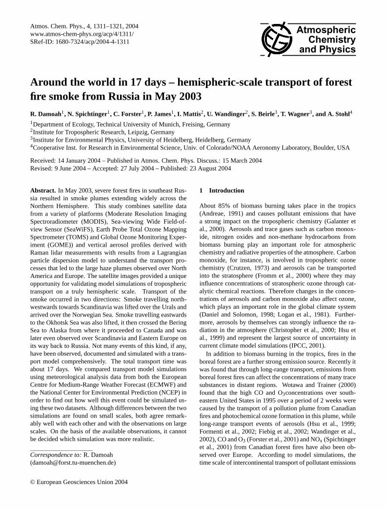
Fig. 1. MODIS fire product for 13, 14, 16 and 31 May, 2003, respectively (left column) and corresponding daily GOME tropospheric NO2(right column).

In order to determine the origin and the transport of theseplumes, we used the Lagrangian particle dispersion modelFLEXPART (Stohl et al., 1998; Stohl and Thomson, 1999) tosimulate the transport of a CO tracer. A CO tracer was usedbecause CO has a relatively long life time that ranges from1 month (in the tropics) to 4 months (in the mid-latitudes)(Seinfeld and Pandis, 1998). As the emphasis in this paper ison the transport, we used a passive tracer (CO) not undergo-ing removal processes so that observed structures will alwaysbe present in the model results for qualitative comparison.

FLEXPART simulates the long-range transport, diffusion,dry and wet deposition and radioactive decay of air pollu-tants released from point, line or volume sources. It treats ad-vection and turbulent diffusion by calculating the trajectoriesof a multitude of particles. Stochastic fluctuations, obtainedby solving Langevin equations (Stohl and Thomson, 1999),are superimposed on the grid-scale winds from global me-teorological datasets to represent transport by turbulent ed-dies, which are not resolved. Global data sets also do notresolve individual convective cells, although they reproduce

the large-scale effects of convection (e.g. the strong ascentwithin WCBs ). Therefore, FLEXPART has recently beenequipped with a convection scheme (Emanuel and Zivkovic-Rothman, 1999) to account for sub-grid scale transport.FLEXPART can be driven by meteorological analysis dataeither from the European Centre for Medium-Range WeatherForecasts (ECMWF, 1995) or from the Global Forecast Sys-tem (GFS) of the National Center for Environmental Predic-tion (NCEP). Simulations using data from both sources weremade in order to possibly find out which dataset provided amore accurate simulation of the transport event.

The ECMWF model version used here has 60 hybridmodel levels in the vertical, while the GFS output is avail-able on 26 pressure levels. In the horizontal, both datasetsare global with a 1◦×1◦ regular grid. 6-hourly analyses aresupplemented by 3-hour forecast step data to provide a 3-hourly temporal resolution in both cases. An output gridwith a 1◦

×2◦ latitude/longitude resolution, a vertical spacingof 1000 m and an output interval of 3 h was employed. Dueto the significantly higher vertical resolution of the ECMWF

www.atmos-chem-phys.org/acp/4/1311/ Atmos. Chem. Phys., 4, 1311–1321, 2004


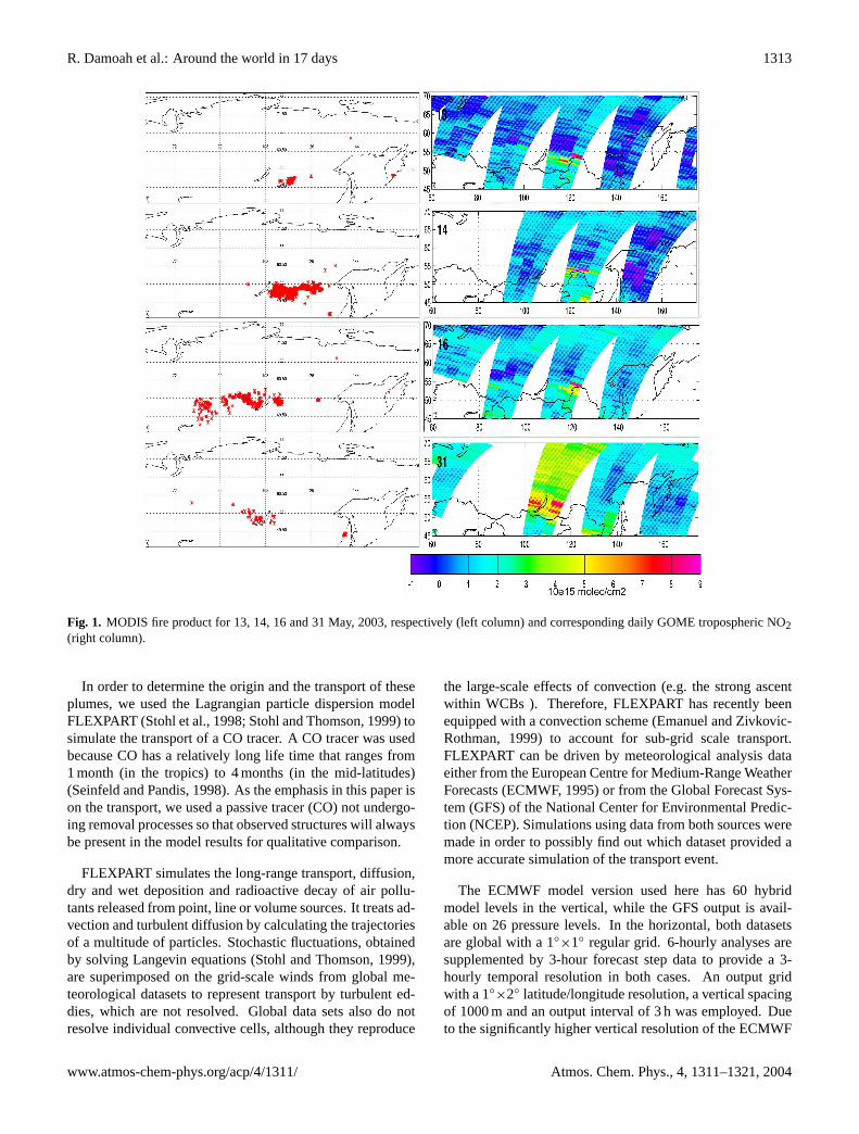
Fig. 2. Total CO tracer columns from simulations using ECMWF data (left column) and GFS data (right columns) on(a) 18 May 2003 at00 UTC,(b) 21 May at 00 UTC,(c) 22 May at 06 UTC,(d) 26 May at 06 UTC and(e)31 May at 00 UTC, respectively.

data grid and the higher intrinsic horizontal resolution of theoperational ECMWF forecast model, compared to the GFSmodel, the simulation based on ECMWF data is our primarysimulation of the smoke transport and will be used to high-light specific transport phenomena. However, the GFS sim-ulation is very useful as a control run to indicate how differ-ences in the meteorological analyses might affect the accu-racy of the transport and its comparison with satellite data.

In the tracer simulations, 5×106 particles were released tocalculate the transport of CO emissions from fires in Russia.For our simulation we considered the 3-week period from 10to 31 May 2003, when the most spectacular long-range trans-port event occurred. Between 10 and 31 May, with approx-imately 0.26×106 ha burning per day, a total area of about5.5×106 ha was burned in Chitinskaya Oblast, Buryatiya Re-pulic and Amurskaya Oblast, according to weekly estimatesof the Global Fire Monitoring Center (GFMC, 2003). In or-der to describe the regional and daily variations of the fires,the MODIS hot spot data (MOD14 product) were used tospatially and temporally disaggregate the total burned areataken from GFMC (2003), assuming that the 10 310 hotspots detected during that period (Fig. 1) all burned an equalarea. CO emissions were taken to be proportional to the areaburned. Assuming a CO release of 4500 kg per hectare offorest burned, which is similar to recent estimates based onemissions from the Canadian Northwest Territories (Cofer etal., 1998), we estimate that 24.75 Tg of CO were released

into the atmosphere due to the burning during May 10 toMay 31 2003. The altitudes at which the emissions were ef-fectively released into the atmosphere vary from day to dayand are actually not known. Lacking this information, wereleased the CO tracer into the lowest 3 km of the modelatmosphere. Sensitivity studies performed on this event byvarying the upper release level from 0.5 km to 4 km altitudedid not change the results much (less than 4% of the globalmean concentration).

3 Results

The left column of Fig. 1 shows Moderate-Resolution Imag-ing Spectroradiometer (MODIS) fire products (MOD14) for13, 14, 16 and 31 May, 2003, respectively. At the exampleof these four days it can be seen that there is a relatively highday-to-day variability, which to some extent may be real, butpartly may also be due to the presence or non-presence ofclouds and/or smoke over the fires. Because we have used thehot spot data to estimate the emissions in our model this mayalso introduce artificial variability into the transport modelsimulations. At the locations of these fires, distinct maximaof GOME’s NO2 tropospheric columns are found (right col-umn). Despite the general agreement between fire locationsand NO2 maxima, the number of the fires does not correlatewell to the strength of the NO2 signal. For instance, on 14May, the hot spots show a strong burning east of Lake Baikal



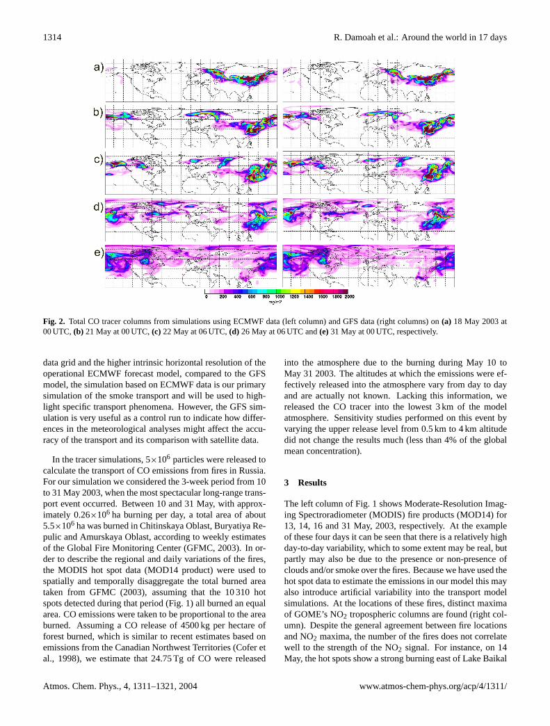
Fig. 3. (a–c)FLEXPART ECMWF CO tracer columns over the Bering Sea and adjacent regions with superimposed contours of the 500 hPageopotential surface, based on GFS analyses, contour interval 5 dam, at (a) 19 May 00 UTC, (b) 20 May 12 UTC and (c) 22 May 00 UTC; Thehatched area represents the topography. Green areas represent land surface, oceans are white. The red rectangle in c) shows approximatelythe area shown in panel d);(d) SeaWiFS image showing smoke over Alaska at 23 UTC on 21 May; Whitish colors are snow, ice and clouds,whereas the blue-grey indicate smoke.(e) vertical section through the FLEXPART CO tracer at 64◦ latitude on 22 May at 00 UTC usingECMWF data.

but relatively low NO2columns were observed over the firesby GOME. On the other hand, fewer hot spots were detectedeast of Lake Baikal on 13 and 31 May, but the GOME NO2enhancements over the fires were much larger. This may bedue to the presence of clouds which hamper both the detec-tion of hot spots and NO2 beneath the clouds, differences inthe temporal coverage of the two intstruments, or may reflect

true variability of the NO2 emissions (for instance, differentemissions strengths during flaming versus smoldering burn-ing condition) and their transport away from their sources.

Before considering the specific meteorological eventswhich were significant for the intercontinental transport ofaerosols from the Russian fires, it is worthwhile looking atthe spread of the pollution with time over the hemisphere.



Figure 2 shows total columns of the CO tracer simulated byFLEXPART using ECMWF (left column) and GFS (rightcolumn) data as input. At around 18 May (Fig. 2a), therewere two main modes of transport, one northwestwardstowards Northern Europe and the other eastwards to theOkhotsk Sea. The CO tracer travelling towards Europewas lifted over the Urals and was heading to Scandinavia(Fig. 2a). Four days later it split up over the NorwegianSea with one part reversing to Asia (Fig. 2c). The moreinteresting to us is the other mode of the transport, whichtook the fire emissions around the globe. The CO tracerwas lifted over the Okhotsk Sea, where it travelled rapidlythrough Alaska (Fig. 2b) to Canada (Fig. 2c), then crossedthe Atlantic to Europe (Fig. 2d) where it began to mergewith the tracer which had been advected directly out of Rus-sia from the east. On 31 May, 2003 the CO tracer couldbe seen over much of the northern hemisphere (Fig. 2e).By this time the plume that had travelled across the Pacificand Atlantic oceans had also indeed crossed Eurasia, takingabout 17 days to circle the entire globe. A closer look atthe two data sets reveals regional differences between sim-ulations using ECMWF and GFS data, respectively. Gener-ally, however, the two simulations were remarkably similarto each other. Both showed the two modes of transport andthe hemispheric-scale transport event.

3.1 Smoke over Alaska (8th day)

During the period 19–22 May, the north Pacific jet was splitinto two components: a southern component near 40◦ N as-sociated with the north Pacific storm track, not relevant tothis discussion, and a zonally elongated polar jet componentstretching from north-east Siberia across the Bering Sea intoAlaska; the latter is shown at 500 hPa in Figs. 3a–c. A largebody of tracer was advected out of Siberia by this strongwesterly flow which was further intensified by the growth oftwo synoptic waves on the jet, which cross the Bering Straitwithin 36 h of each other (Figs. 3b and c). The first of thesewaves cuts off the leading edge of the plume which is thenadvected quickly into northwestern Canada. The main bodyof the plume is pushed by the second wave over Alaska andhas been very well simulated by the FLEXPART CO tracerusing both ECMWF (Fig. 3c) and GFS data (not shown). On21 May 2003, Sea WiFS captured an aerosol plume (Fig. 3d)over Alaska that was presumably transported from the in-tense forest fire burning in Russia. Images from the MOPITT(Measurement Of Pollution In The Troposphere) instrument(not shown) studied within this period also shows forest fireemissions (Edwards et al., 2003) over Alaska. When com-paring this available satellite image. In particular, the sharpedges of the plume in the image over the Gulf of Alaska,westwards to the Aleutians and then northwards over theBering Sea, coincide well with the edges of the CO tracerplume. A vertical section through the FLEXPART-ECMWFCO tracer at 64◦ N indicates that the main plume over Alaska

is concentrated between 2 and 5 km altitude while the ad-vanced plume over northwestern Canada is somewhat higher,primarily lying between 4 and 7 km. Clouds in Fig. 3d aremostly at lower altitudes, partly lying underneath the smoke.

3.2 Smoke over Canada (11th day)

On 21 May a smoke plume which arrived first overnorth-western Canada (see description above) was advectedquickly south-eastwards before arriving and becoming slow-moving near the Great Lakes in a diffluent mid-troposphericflow on 23 May. On 24 May 2003 (Fig. 4c) simulatedFLEXPART CO tracer showed elongated plumes whichstretches from the north-western edge of Lake Superior uptowards James Bay and reaches across to Quebec and theSt. Lawrence River. The plume coincides well with the im-age of MODIS instrument aboard the Terra satellite whichalso showed elongated smoke plumes (Figs. 4a and b) on 23and 24 May. An anticyclonic ridge builds between the po-lar cylconic vortex and a small new cut-off low which de-velops quickly to the south of the Great Lakes. As a result,the plume is stretched out and its western flank is advectedaround the developing low south- and eastwards into the east-ern United States. Meanwhile its eastern flank is pulled outby strong westerly winds past the southern tip of Greenlandand reaches Iceland by 24 May (Figs. 4c and d).

Another smoke maximum is indicated over part of Mani-toba on 23 May in the upper left corner of Fig. 4a. This is theedge of the main plume body which was seen over Alaska on22 May (Fig. 3c) and moved into Canada about 48 h behindthe leading plume above. This large main plume is advectedin the strong westerly flow and arrives over the Hudson Bayon 25 May, where much of it slows down as it comes underthe influence of diffluent flow ahead of a developing ridge.The leading edge of this plume, however, is pulled away fromthe rest in two bursts by strong flow on the edge of a troughcentred over Baffin Island. One part is advected northwardsto western Greenland on 24 May (Fig. 4d) and another overthe Labrador Sea on 25 May (Fig. 4e).

Figure 4f shows the TOMS aerosol index on 24 May. Italso shows a maximum over Hudson Bay and a filamentstretching from south-east of James Bay to the St. Lawrenceriver, in fairly good agreement with the FLEXPART tracersimulation. However, no significant aerosols registered inTOMS near Lake Superior. This can be partly attributed tothe dissipation of the smoke in this region later on 24 May(note that local midday, significant for TOMS measurements,was after 18 UTC) or the possible presence of clouds.

3.3 Smoke over Scandinavia (14th day)

The rapid advection of the plume across the Atlantic wascaused by the development of a small but intense and mo-bile synoptic wave and associated strong winds near Icelandon 25 May (Fig. 5a). This wave moves quickly eastwards



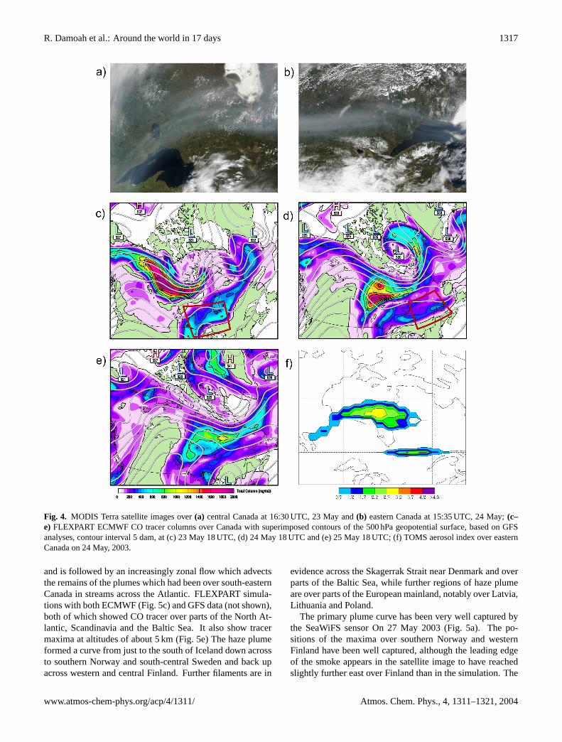
Fig. 4. MODIS Terra satellite images over(a) central Canada at 16:30 UTC, 23 May and(b) eastern Canada at 15:35 UTC, 24 May;(c–e) FLEXPART ECMWF CO tracer columns over Canada with superimposed contours of the 500 hPa geopotential surface, based on GFSanalyses, contour interval 5 dam, at (c) 23 May 18 UTC, (d) 24 May 18 UTC and (e) 25 May 18 UTC; (f) TOMS aerosol index over easternCanada on 24 May, 2003.

and is followed by an increasingly zonal flow which advectsthe remains of the plumes which had been over south-easternCanada in streams across the Atlantic. FLEXPART simula-tions with both ECMWF (Fig. 5c) and GFS data (not shown),both of which showed CO tracer over parts of the North At-lantic, Scandinavia and the Baltic Sea. It also show tracermaxima at altitudes of about 5 km (Fig. 5e) The haze plumeformed a curve from just to the south of Iceland down acrossto southern Norway and south-central Sweden and back upacross western and central Finland. Further filaments are in

evidence across the Skagerrak Strait near Denmark and overparts of the Baltic Sea, while further regions of haze plumeare over parts of the European mainland, notably over Latvia,Lithuania and Poland.

The primary plume curve has been very well captured bythe SeaWiFS sensor On 27 May 2003 (Fig. 5a). The po-sitions of the maxima over southern Norway and westernFinland have been well captured, although the leading edgeof the smoke appears in the satellite image to have reachedslightly further east over Finland than in the simulation. The



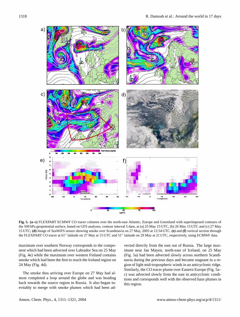
Fig. 5. (a–c)FLEXPART ECMWF CO tracer columns over the north-east Atlantic, Europe and Greenland with superimposed contours ofthe 500 hPa geopotential surface, based on GFS analyses, contour interval 5 dam, at (a) 25 May 15 UTC, (b) 26 May 15 UTC and (c) 27 May15 UTC;(d) Image of SeaWiFS sensor showing smoke over Scandinavia on 27 May, 2003 at 12:54 UTC.(e)and(f) vertical section throughthe FLEXPART CO tracer at 61◦ latitude on 27 May at 15 UTC and 51◦ latitude on 29 May at 21 UTC, respectively, using ECMWF data.

maximum over southern Norway corresponds to the compo-nent which had been advected over Labrador Sea on 25 May(Fig. 4e) while the maximum over western Finland containssmoke which had been the first to reach the Iceland region on24 May (Fig. 4d).

The smoke thus arriving over Europe on 27 May had al-most completed a loop around the globe and was headingback towards the source region in Russia. It also began in-evitably to merge with smoke plumes which had been ad-

vected directly from the east out of Russia. The large max-imum near Jan Mayen, north-east of Iceland, on 25 May(Fig. 5a) had been advected slowly across northern Scandi-navia during the previous days and became stagnant in a re-gion of light mid-tropospheric winds in an anticyclonic ridge.Similarly, the CO tracer plume over Eastern Europe (Fig. 5a–c) was advected slowly from the east in anticyclonic condi-tions and corresponds well with the observed haze plumes inthis region.



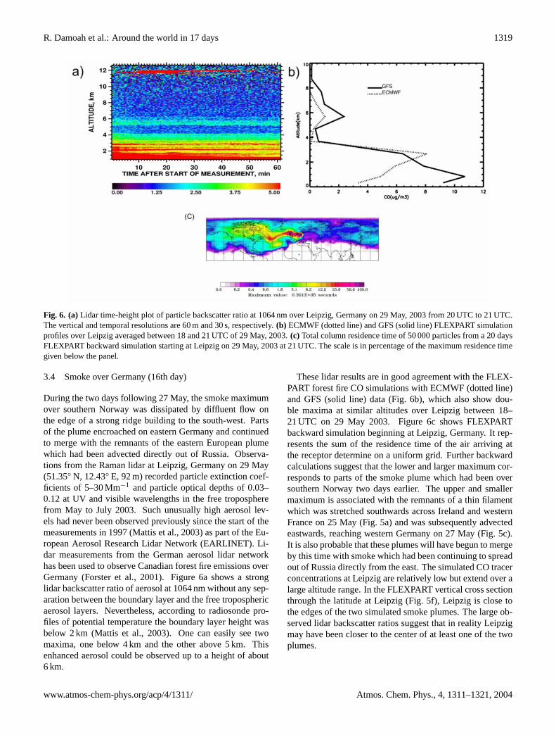
Fig. 6. (a)Lidar time-height plot of particle backscatter ratio at 1064 nm over Leipzig, Germany on 29 May, 2003 from 20 UTC to 21 UTC.The vertical and temporal resolutions are 60 m and 30 s, respectively.(b) ECMWF (dotted line) and GFS (solid line) FLEXPART simulationprofiles over Leipzig averaged between 18 and 21 UTC of 29 May, 2003.(c) Total column residence time of 50 000 particles from a 20 daysFLEXPART backward simulation starting at Leipzig on 29 May, 2003 at 21 UTC. The scale is in percentage of the maximum residence timegiven below the panel.

3.4 Smoke over Germany (16th day)

During the two days following 27 May, the smoke maximumover southern Norway was dissipated by diffluent flow onthe edge of a strong ridge building to the south-west. Partsof the plume encroached on eastern Germany and continuedto merge with the remnants of the eastern European plumewhich had been advected directly out of Russia. Observa-tions from the Raman lidar at Leipzig, Germany on 29 May(51.35◦ N, 12.43◦ E, 92 m) recorded particle extinction coef-ficients of 5–30 Mm−1 and particle optical depths of 0.03–0.12 at UV and visible wavelengths in the free tropospherefrom May to July 2003. Such unusually high aerosol lev-els had never been observed previously since the start of themeasurements in 1997 (Mattis et al., 2003) as part of the Eu-ropean Aerosol Research Lidar Network (EARLINET). Li-dar measurements from the German aerosol lidar networkhas been used to observe Canadian forest fire emissions overGermany (Forster et al., 2001). Figure 6a shows a stronglidar backscatter ratio of aerosol at 1064 nm without any sep-aration between the boundary layer and the free troposphericaerosol layers. Nevertheless, according to radiosonde pro-files of potential temperature the boundary layer height wasbelow 2 km (Mattis et al., 2003). One can easily see twomaxima, one below 4 km and the other above 5 km. Thisenhanced aerosol could be observed up to a height of about6 km.

These lidar results are in good agreement with the FLEX-PART forest fire CO simulations with ECMWF (dotted line)and GFS (solid line) data (Fig. 6b), which also show dou-ble maxima at similar altitudes over Leipzig between 18–21 UTC on 29 May 2003. Figure 6c shows FLEXPARTbackward simulation beginning at Leipzig, Germany. It rep-resents the sum of the residence time of the air arriving atthe receptor determine on a uniform grid. Further backwardcalculations suggest that the lower and larger maximum cor-responds to parts of the smoke plume which had been oversouthern Norway two days earlier. The upper and smallermaximum is associated with the remnants of a thin filamentwhich was stretched southwards across Ireland and westernFrance on 25 May (Fig. 5a) and was subsequently advectedeastwards, reaching western Germany on 27 May (Fig. 5c).It is also probable that these plumes will have begun to mergeby this time with smoke which had been continuing to spreadout of Russia directly from the east. The simulated CO tracerconcentrations at Leipzig are relatively low but extend over alarge altitude range. In the FLEXPART vertical cross sectionthrough the latitude at Leipzig (Fig. 5f), Leipzig is close tothe edges of the two simulated smoke plumes. The large ob-served lidar backscatter ratios suggest that in reality Leipzigmay have been closer to the center of at least one of the twoplumes.



4 Conclusions

In this paper, we investigated the transport of smoke fromRussian boreal forest fires from 10 to 31 May, 2003 using theLagrangian dispersion model, FLEXPART, comparing simu-lations based on ECMWF and GFS meteorological data.

The transport of the smoke plumes was unique in the sensethat, within 17 days, smoke had circumnavigated the globe:perhaps the first time this has been so clearly documented.From the source, smoke crossed the Bering Sea to Alaska,where it was visible in SeaWiFS imagery and then quicklycrossed to eastern Canada, where the MODIS Terra satellitewitnessed it. It proceeded across the Atlantic to Europe, ascaptured in a further SeaWiFS image, on its way back to Rus-sia and began to merge over Europe with smoke which hadbeen advected directly out of Russia westwards. By the endof May 2003 the plume had engulfed much of the NorthernHemisphere. The fact that haze plumes from boreal forestfires can circumnavigate the globe and can persist for longerthan two weeks has large implications for the radiative heat-ing of the atmosphere (Fiebig et al., 2002). Not accountingfor such plumes in climate model simulations or numericalweather predictions may possibly lead to large errors.

FLEXPART simulations based on both ECMWF and GFSdata could reproduce much of the fine-scale structure seenin the satellite images with remarkable accuracy, even afterthe smoke plume had travelled almost around the northernhemisphere. It is not clear from our results which of the twosimulations is in better agreement with the observations.

Acknowledgements.We acknowledge ECMWF and the GermanWeather Service for permitting access to the ECMWF archivesand also NCEP for the GFS data. We appreciate the provi-sion of data via the internet by the science teams of MODIS,TOMS and SeaWiFS. This study was funded by the EuropeanCommission in the European Research Framework 5 programas part of the PARTS (no. EVK2CT200100112) project and theGerman Federal Ministry for Education and Research in theFramework of the Atmospheric Research 2000 program as part ofthe NOXTRAM (07 ATF05) and ATMOFAST (07 ATF08) projects.

Edited by: A. Hofzumahaus

References

Andreae, M. O.: Biomass burning: Its history, use and distributionand its impact on environmental quality and global climate, inGlobal Biomass Burning: Atmospheric, Climate, and BiosphericImplications, edited by Levine, J. S., pp. 3–21, MIT Press, Cam-bridge, Mass, 1991.

Andreae, M. O. and Merlet, P.: Emissions of trace gases andaerosols from biomass burning, Global Biogeochem. Cycles, 15,955–977, 2001.

Beirle, S., Platt, U., Wenig, M., and Wangner, T.: Weekly cycleof NO2 by GOME measurements: a signature of anthropogenicsources, Atmos. Chem. Phys., 3, 2225–2232, 2003.

Cahoon, D. R., Stocks, B. J, Levine, J. S., Cofer III, W. R., andPierson, J. M.: Satellite analysis of the severe 1987 forest firesin northern China and southeastern Siberia, J. Geophys. Res., 99,18 627–18 638, 1994.

Christopher, S., Chou, J., Chang, J., Lin, X., Berendes, T. A., andWelch, R. M.: Shortwave direct radiative forcing of biomassburning aerosols estimated using VIRS and CERES data, Geo-phys. Res. Lett., 27, 2197–2200, 2000.

Chu, D. A., Kaufman, Y. J., Ichoku, C., Remer, L. A., Tanre,D., and Holben, B. N.: Validation of MODIS aerosols op-tical depth retrieval over land, Geophys. Res. Lett., 29, 12,doi:10.1029/2001GL013205, 2002.

Cofer, W. R., Winstead, E. L., Stocks, B. J., Goldammer, J. G., andCahoon, D. R.: Crown fire emissions of CO2, CO, H2, CH4, andTNMHC from dense jack pine boreal forest fire, Geophys. Res.Lett., 25, 3919–3922, 1998.

Conard, S. G. and Ivanova, G. A. : Wildfire in Russian boreal forests– potential impacts of fire regime characteristics on emissionsand global carbon estimates, Envir. Pol., 98, 305–313, 1998.

Conard, S. G., Sukhinin, A. I., Stocks, B.J., Cahoon, D. R., Davi-denko, E. P., and Ivanova, G. A.: Determining effects of areaburned and fire severity on carbon cycling and emissions inSiberia, Climate Change, 55, 197–211, 2002.

Crutzen, P. J.: A discussion of the chemistry of some minor con-stituents in the stratosphere and troposphere, Pure Appl. Geo-phys., 106–108, 1385–1399, 1973.

Daniel, J. S. and Solomon, S.: On the climate forcing of carbonmonoxide, J. Geophys. Res., 103, 13 249–13 260, 1998.

ECMWF: User Guide to ECMWF Products 2.1, Meteorol. Bull.M3.2, ECMWF, Reading, UK, 1995.

Edwards, D. P., Lamarque, J.-F., Attie, J.-L., Emmons, L. K.,Richter, A., Cammas, J.-P., Gille, J. C., Francis, G. L., Deeter,M. N., Warner, J., Ziskin, D. C., Lyjak, L. V., Drummond, J.R., and Burrows, J. P.: Tropospheric ozone over the tropicalAtlantic: A satellite perspective, J. Geophys. Res., 108, 4237,doi:10.1029/2002JD002927, 2003.

Emanuel, K. A. and Zivkovic-Rothman, M.: Development and eval-uation of a convection scheme for use in climate models, J. At-mos. Sci., 56, 1766–1782, 1999.

Fiebig, M., Petzold, A., Wandinger, U., Wendisch, M., Kiemle, C.,Stifter, A., Ebert, M., Rother, T., and Leiterer, U.: Optical closurefor an aerosol column: Method, accuracy, and inferable proper-ties applied to a biomass-burning aerosol and its radiative forc-ing, J. Geophys. Res., 107, 8130, doi:10.1029/2000JD000192,2002.

Formenti, P., Reiner, T., Wendisch, M., et al.: : STAAARTE-MED1998 summer airborne measurements over the Aegean Sea, 1,Aerosol particles and trace gases, J. Geophys. Res., 107, 4450,doi:10.1029/2001JD001337, 2002.

Forster, C., Wandinger, U., Wotawa, G., James, P., Mattis, I., Al-thausen, D., Simmonds, P., O’Doherty, S., Jennings, S., Kleefeld,C., Schnieder, J., Trickl, T., Kreipl, S., Jager, H., and Stohl, A.:Transport of boreal forest fire emissions from Canada to Europe,J. Geophys. Res., 106, 22 887–22 906, 2001.

Fromm, M., Alfred, J., Hoppel, K., Hornstein, J., Bevilacqua, R.,Shettle, E., Servranckx, R., Li, Z., and Stocks, B.: Observa-tions of boreal forest fire smoke in the stratosphere by POAMIII, SAGE II, and lidar in 1998, Geophys. Res. Lett., 27, 1407–1410, 2000.



Fromm, M. D. and Servranckx, R.: Transport of forest fire smokeabove the tropopause by supercell convection, Geophys. Res.Lett., 30, 1542, doi: 1029/2002GL016820, 2003.

Galanter, M., Levy II, H., and Carmichael, G. R.: Impacts ofbiomass burning on tropospheric CO, NOx, and O3, J. Geophys.Res., 105, 6633–6653, 2000.

Global Fire Monitoring Center (GFMC): Daily/weekly updatesof forest fires in the Russian Federation, http://www.fire.uni-freiburg.de/current/globalfire.htm, 2003.

Gordon, H. R. and Wang M.: Retrieval of water-leaving radianceand aerosol optical thickness over the oceans with SeaWiFS: apreliminary algorithm, Appl. Opt., 33, 443–452, 1994.

Hooker, S. B., Mcclain, C. R., and Holmes, A.: Ocean color imag-ing – Costal Zone Color Scanner (CZCS) to Sea WiFS, MarineTechnology Society Journal, 27, 3–15, SPR, 1993.

Hsu, N. C., Herman, J., Gleason, J., Torres, O., and Seftor, C.:Satellite detection of smoke aerosols over a snow/ice surface byTOMS, Geophys. Res. Lett. 26, 1165–1168, 1999.

IPCC: Climate Change, edited by Nebojsa Nakicenovic and RobSwart, Cambridge Univ. Press, New York, 2001.

Justice, C. O., Kendall, J. D., Dowty, P. R., and Scholes, R.: Satel-lite remote sensing of fires during the SAFARI campaign usingNOAA advanced very high radiometer data, J. Geophys. Res.,101, 23 851–23 863, 1996.

Kasischke, E. S., Stocks, B. J., Oneill, K., French, N. H., andBourgeau-Chavez, L. L.: Direct effects of fire on the boreal forestcarbon budget, in Biomass burning and its Inter – Relationshipswith the Climate System, edited by Innes, J. L., Beniston, M.,and Verstraete, M. M., pp. 51–68, Kluwer Academic Publishers,Dordrecht, Netherlands, 2000.

Kasischke, E. S. and Bruhwiler, L. P.: Emissions of carbon dioxide,carbon monoxide, and methane from boreal forest fires in 1998,J. Geophys. Res., 108, 8146, doi:10.1029/2001JD000461, 2003.

Kaufman, Y. J., Justice, C. O., Flynn, L. P., Kendall, J. D., Prins,E. M., Giglio, L., Ward, D. E., Menzel, W. P., and Setzer, A. W.:Potential global fire monitoring from EOS-MODIS, J. Geophys.Res., 103, 32 215–32 238, 1998.

Kaufman, Y. J., Ichoku, C., Giglio, L., Korontzi, S., Chu, D. A.,Hao, W. M., Li, R.-R., and Justice, C. O.: Fire and smoke ob-served from Earth Observing System MODIS instrument – prod-ucts, validation, and operational use, Int. J. Remote Sensing, 24,1765–1781, 2003.

Lavoue, D. C., Liousse, C., Cachier, H., Stocks, B. J., andGoldammer, J. G.: Modelling of carbonaceous particles emittedby boreal and temperate wildfires at northern latitudes, J. Geo-phys. Res., 105, 26 871–26 890, 2000.

Logan, J. A., Prather, M. J., Wofsy, S. C., and McElroy, M. B.:Tropospheric chemistry: A global perspective, J. Geophys. Res.,86, 7210–7254, 1981.

Mattis, I., Ansmann, A., Wandinger, U., and Muller, D.: Unex-pectedly high aerosol load in the free troposphere over CentralEurope in spring/summer 2003, Geophys. Res. Lett., 30, 2178,doi:10.1029/2003GL018442, 2003.

Platt, U.: Differential optical absorption spectroscopy (DOAS), inair monitoring by spectroscopic techniques, M. W. Sigrist (Ed.),Chemical Analysis Series vol. 127, John Wiley, New York, 1994.

Remer, L. A., Tanre, D., Kaufman, Y. J., Ichoku, C., Mattoo, S.,Levy, R., Chu, D. A., Holben, B. N., Dubovik, O., Ahmad,Z., Smirnov, A., Martins, J. V., and Li, R.-R.: Validation ofMODIS aerosol retrieval over ocean. Geophys. Res. Lett. 29, 12,doi:10.1029/2001GL013204, 2002.

Seinfeld, J. H. and Pandis, S. N.: Atmospheric Chemistry andPhysics, 1326pp., John Wiley, Inc., New York, 1998.

Shvidenko, A. Z., and Nilsson, S.: Fire and the carbon budget ofRussian forest, in Fire, Climate Change, and Carbon Cycling inthe Boreal Forest, edited by E. S. Kasischke, Ecol. Stud., 138,289–311, 2000

Shvidenko, A. and Goldammer, J. G.: Fire situation in Russia, In-ternational Forst Fire News, 24, 41–59, 2001.

Soja, A. J., Sukhinin, A. I., Cahoon, D. R., Shugart, H. H., andStackhouse, P. W.; AVHRR-derived fire frequency, distributionand area burned in Siberia, Int. J. Remote Sensing, 25, 1939–1960, 2004.

Spichtinger, N., Wenig, M., James, P., Wagner, T., Platt, U., andStohl, A.: Satellite detection of a continental-scale plume of ni-trogen oxides from boreal forest fires, Geophys. Res. Lett., 28,4579–4583, 2001.

Stohl, A., Hittenberger, M., and Wotawa, G.: Validation of theLagrangian particle dispersion model FLEXPART against largescale tracer experiment data, Atmos. Environ., 24, 4245–4264,1998.

Stohl, A. and Trickl, T.: A textbook example of long-range trans-port: Simultaneous observation of ozone maxima of strato-spheric and North American origin in the free troposphere overEurope, J. Geophys. Res., 104, 30 445–30 462, 1999.

Stohl, A. and Thomson, D. J.: A density correction for Lagrangianparticle dispersion models, Boundary-Layer Meteorol., 90, 155–167, 1999.

Stohl, A.: A one-year Lagrangian climatology of airstreams in thenorthern hemisphere troposphere and lowermost stratosphere, J.Geophys. Res., 106, 7263–7279, 2001.

Stohl, A., Eckhardt, S., Forster, C., James, P., and Spichtinger,N.: On the pathways and timescales of intercontinen-tal air pollution transport, J. Geophys. Res., 107, 4684,doi:10.1029/2001JD001396, 2002.

Valendick, E. N.: Ecological aspects of forest fires in Siberia, Sib.Ecol. J., 1, 1–8, 1996.

Wandinger, U., Bockmann, C., Mathias, V., et al.: Opti-cal and microphysical characterization of biomass- burningand industrial-pollution aerosols from multiwavelength lidarand aircraft measurements, J. Geophys. Res., 107, 8125,doi:10.1029/2000JD000202, 2002.

Wotawa, G. and Trainer, M.: The influence of Canadian forest fireson pollutant concentrations in the United States, Science, 288,324–328, 2000.

Yoshizumi, K., Kato, S., Streets, D. G., Tsai, Y. N., Shvidenko,A., Nilsson, S., McCallum, I., Minko, N. P., Abushenko, N., Al-tyntsev, D., and Khodzer, T. V.: Boreal forest fires in Siberia in1998: Estimation of area burned and emissions of pollutants byadvanced very high resolution radiometer satellite data, J. Geo-phys. Res., 107, 4745, doi:10.1029/2001JD001078, 2002.


around the world in 17 days – hemispheric-scale … · and physics around the world in ... ﬁre...

Documents