arrhythmia classification in multi-channel ecg signals ...using a dataset of 106 patient readings,...

Arrhythmia Classification in Multi-Channel ECG SignalsUsing Deep Neural Networks

Kyungna Kim

Electrical Engineering and Computer SciencesUniversity of California at Berkeley

Technical Report No. UCB/EECS-2018-80http://www2.eecs.berkeley.edu/Pubs/TechRpts/2018/EECS-2018-80.html

May 19, 2018

Copyright © 2018, by the author(s).All rights reserved.

Permission to make digital or hard copies of all or part of this work forpersonal or classroom use is granted without fee provided that copies arenot made or distributed for profit or commercial advantage and that copiesbear this notice and the full citation on the first page. To copy otherwise, torepublish, to post on servers or to redistribute to lists, requires prior specificpermission.

Arrhythmia Classification in Multi-Channel ECG Signals Using Deep NeuralNetworks

Copyright 2018by

Kyungna Kim

1

Abstract

An important diagnostic tool in identifying heart rhythm irregularities, known as arrhyth-mias, is the electrocardiogram (ECG). Accurate identification of arrhythmias is critical topatient well-being in clinical settings, as both acute and chronic heart conditions are typ-ically reflected in these readings. This is known to be a difficult problem even for humanexperts, due to variability between individuals and inevitable noise. We explore the use ofdeep neural networks for the task of classifying ECG recordings using recurrent and residualarchitectures. Using a dataset of 106 patient readings, we train several deep networks tocategorize slices of ECG data into one of six classes, including normal sinus rhythm, arti-fact/noise, and four arrhythmias of varying levels of severity. We investigate the usefulnessof multi-channel ECG data without additional feature extraction in this problem, especiallywhen common frequency domain transformation feature representation may not be suitabledue to low periodicity of data.

i

Contents

Contents i

List of Figures ii

List of Tables iii

1 Introduction 1

2 Background 32.1 Cardiac Arrhythmias . . . . . . . . . . . . . . . . . . . . . . . . . . . . . . . 32.2 Related Work . . . . . . . . . . . . . . . . . . . . . . . . . . . . . . . . . . . 5

3 Methods 73.1 Data . . . . . . . . . . . . . . . . . . . . . . . . . . . . . . . . . . . . . . . . 73.2 Model Architectures . . . . . . . . . . . . . . . . . . . . . . . . . . . . . . . 83.3 Metrics . . . . . . . . . . . . . . . . . . . . . . . . . . . . . . . . . . . . . . . 12

4 Experiments and Results 144.1 Setup . . . . . . . . . . . . . . . . . . . . . . . . . . . . . . . . . . . . . . . . 144.2 Training . . . . . . . . . . . . . . . . . . . . . . . . . . . . . . . . . . . . . . 154.3 Results . . . . . . . . . . . . . . . . . . . . . . . . . . . . . . . . . . . . . . . 15

5 Conclusions and Future Work 195.1 Limitations . . . . . . . . . . . . . . . . . . . . . . . . . . . . . . . . . . . . 195.2 Future Work . . . . . . . . . . . . . . . . . . . . . . . . . . . . . . . . . . . . 21

References 22

ii

List of Figures

2.1 Examples of rhythm types . . . . . . . . . . . . . . . . . . . . . . . . . . . . . . 42.2 Single vs multi-channel data . . . . . . . . . . . . . . . . . . . . . . . . . . . . . 5

3.1 An LSTM unit . . . . . . . . . . . . . . . . . . . . . . . . . . . . . . . . . . . . 93.2 Bidirectional LSTM network with 2 stacked layers . . . . . . . . . . . . . . . . . 103.3 Residual network . . . . . . . . . . . . . . . . . . . . . . . . . . . . . . . . . . . 113.4 Combined LSTM-CNN model (LSTM portion may be uni- or bidirectional) . . . 12

4.1 Scaled confusion matrices . . . . . . . . . . . . . . . . . . . . . . . . . . . . . . 174.2 Residual network accuracy and loss curves . . . . . . . . . . . . . . . . . . . . . 174.3 BDLSTM-CNN accuracy and loss curves . . . . . . . . . . . . . . . . . . . . . . 18

5.1 Mislabeled data . . . . . . . . . . . . . . . . . . . . . . . . . . . . . . . . . . . . 20

iii

List of Tables

3.1 ECG dataset profile . . . . . . . . . . . . . . . . . . . . . . . . . . . . . . . . . 8

4.1 Aggregate accuracy for all classes (multi-channel) . . . . . . . . . . . . . . . . . 154.2 F1 score comparison over classes . . . . . . . . . . . . . . . . . . . . . . . . . . 164.3 Recall, precision, specificity, F1 score comparison over classes . . . . . . . . . . . 164.4 F1 score for single-channel versus multi-channel data . . . . . . . . . . . . . . . 16

iv

Acknowledgments

I thank my advisor, Professor Russell, for his expertise and guidance during my years at UCBerkeley. I also thank Professor Canny for being second reader.

This would not have been possible without the help of my mentors; many thanks toParia Rashidinejad, my closest collaborator, for her advice and support over the duration ofmy graduate career. I also thank Yusuf Bugra Erol for initially introducing me to medicalapplications of machine learning when I was an undergraduate, and the subsequent projectsthat led to this study.

Lastly, I thank my friends and family for their unending encouragement and support.

1

Chapter 1

Introduction

An important diagnostic tool in identifying chronic and acute heart rhythm irregularities(cardiac arrhythmias) is the electrocardiogram (ECG), which measures electrical heart ac-tivity via electrodes placed on a patient’s skin. ECGs are ubiquitous in intensive care units(ICUs), where clinicians must be able to make critical care decisions quickly and accurately.The ability to correctly distinguish various arrhythmias from each other is crucial for patientwell-being; in many cases, the wave morphologies of benign and lethal arrhythmias can bedifficult to distinguish.

Existing monitoring systems for ECGs record a myriad of vital signs and also utilizealgorithms to determine changes in cardiac rhythm. However, accurate identification ofarrhythmias is known to be challenging even for medical professionals, and requires con-siderable medical expertise. A study investigating diagnostic accuracy for licensed generalpractitioners showed a specificity of 92% and sensitivity of only 80% in distinguishing atrialfibrillation from healthy sinus rhythms [1]. Waveforms often show variation given an indi-vidual’s unique biological characteristics, even for arrhythmias whose identifying patternsare known and well-documented.

ECG recordings also suffer from several potential sources of considerable noise, includingdevice power interference (as the measurements themselves are voltages), baseline drift, con-tact noise between the skin and the electrode, and motion artifacts. These motion artifacts,in particular, can be caused by any muscular activity from the patient; even innocuous move-ment can be mistakenly registered as arrhythmia. Many of our data points are classified asartifacts due to lead failure, excessive measurement noise, or even unclassifiable arrhythmia.

The combination of inter-patient variability and noise makes this a challenging algo-rithmic classification problem, and a variety of methods have been proposed to increasediagnostic accuracy. Standard regression and feed-forward neural network models have beenexplored in the past, and more recent approaches also utilize deep CNN or RNN structures.Feature engineering and spectral analysis are also popular methods for adding or replacingfeatures, though this often limits the scope of the classification.

To exploit the inherently time-dependent nature of ECG readings, we investigate the useof LSTM networks, commonly used to classify or generate sequential data, to distinguish

CHAPTER 1. INTRODUCTION 2

normal sinus rhythm from artifacts and several arrhythmias of varying levels of severity. Inaddition, we explore a combined architecture that includes residual connections, which havebeen have shown to improve classification performance without the significant increase inmodel complexity typically seen in deep learning architectures.

As we have access to multi-channel data, we incorporate this increased dimensionalityinto our algorithm, in contrast to the single-channel input format commonly used in ECGclassification. Individual channels record cardiac electrical activity from various spatial an-gles, and the use of multiple channels is likely to give deeper insight into any underlyingpatterns of arrhythmia that can be interpreted by our model.

We train two baseline models: a single-layer, unidirectional LSTM, and a convolutionalneural network without residual connections. We then train models from three categories(LSTM only, residual networks, and LSTM-CNN combined networks), for a total of sixmodels not including our baseline models.

All models exceed baseline performance on training, validation, and test accuracy. A2-layer, bidirectional LSTM achieves the best performance overall; though networks withresidual structures achieve higher training accuracy, their validation and test accuracies arelower than those of the LSTM only networks. The overall F1 score of 0.803 achieved by thisnetwork exceeds reported cardiologist F1 scores reported in [2].

3

Chapter 2

Background

2.1 Cardiac Arrhythmias

The rhythm of a human heart is regulated by electrical signals produced by two nodeswithin the heart and conducted through a series of specialized cardiac cells. During healthy,normal operation, this occurs at regular intervals and the electrical signal, which causes theheart muscles to contract, propagates via the cardiac electrical conduction system along thecorrect path through the atria and ventricles.

Cardiac arrhythmia occurs when the heartbeat is too fast (tachycardia), too slow (brady-cardia), or altogether abnormal. Both atrial and ventricular arrhythmias can have any num-ber of causes, including scar tissue from previous trauma (such as myocardial infarction)and coronary disease, and can even occur in healthy hearts. Though many arrhythmias areasymptomatic, those that are not can cause symptoms as mild as occasional palpitations oras severe as stroke and sudden cardiac death. As arrhythmias are caused by disorders of theelectrical conduction system, they are reflected in ECG readings as abnormal waveforms.

The complexity of this system often necessitates that clinicians use anywhere from six totwelve ECG leads to capture electrical activity across multiple spatial planes [3]. A singlelead only provides a ‘projection’ of this activity across one specific plane and may not provideenough information to make accurate diagnoses of underlying pathologies.

The rhythms we aim to classify are normal (sinus) rhythm, noise/artifact (or otherwiseunidentifiable arrhythmia), ventricular tachycardia (VT), atrial fibrillation (AF), bigeminy,and premature ventricular contraction (PVC). An example of each class is shown in figure2.1; only one channel is plotted for clarity.

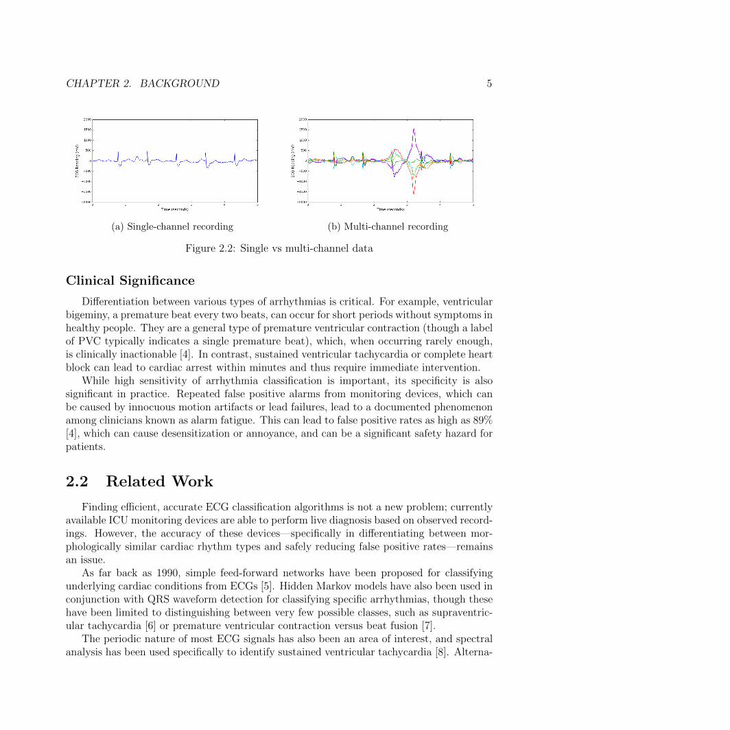
Figure 2.2 presents a case where using multiple channels is key to correct classification.While the single channel recording in 2.2a implies a normal (albeit slightly noisy) sinusrhythm, the full multi-channel recording of the same data point in 2.2b shows a large,abnormal wave about 3 seconds in. This is labeled as an artifact in our dataset; had weconsidered only the data shown in 2.2a, this would have likely been classified as ‘sinus’.

CHAPTER 2. BACKGROUND 4

(a) Sinus/normal (b) Artifact

(c) Ventricular tachycardia (d) Atrial fibrillation

(e) Ventricular bigeminy (f) Premature ventricular contraction

Figure 2.1: Examples of rhythm types


(a) Single-channel recording (b) Multi-channel recording

Figure 2.2: Single vs multi-channel data

Clinical Significance

Differentiation between various types of arrhythmias is critical. For example, ventricularbigeminy, a premature beat every two beats, can occur for short periods without symptoms inhealthy people. They are a general type of premature ventricular contraction (though a labelof PVC typically indicates a single premature beat), which, when occurring rarely enough,is clinically inactionable [4]. In contrast, sustained ventricular tachycardia or complete heartblock can lead to cardiac arrest within minutes and thus require immediate intervention.

While high sensitivity of arrhythmia classification is important, its specificity is alsosignificant in practice. Repeated false positive alarms from monitoring devices, which canbe caused by innocuous motion artifacts or lead failures, lead to a documented phenomenonamong clinicians known as alarm fatigue. This can lead to false positive rates as high as 89%[4], which can cause desensitization or annoyance, and can be a significant safety hazard forpatients.

2.2 Related Work

Finding efficient, accurate ECG classification algorithms is not a new problem; currentlyavailable ICU monitoring devices are able to perform live diagnosis based on observed record-ings. However, the accuracy of these devices—specifically in differentiating between mor-phologically similar cardiac rhythm types and safely reducing false positive rates—remainsan issue.

As far back as 1990, simple feed-forward networks have been proposed for classifyingunderlying cardiac conditions from ECGs [5]. Hidden Markov models have also been used inconjunction with QRS waveform detection for classifying specific arrhythmias, though thesehave been limited to distinguishing between very few possible classes, such as supraventric-ular tachycardia [6] or premature ventricular contraction versus beat fusion [7].

The periodic nature of most ECG signals has also been an area of interest, and spectralanalysis has been used specifically to identify sustained ventricular tachycardia [8]. Alterna-


tive time-frequency distributions to Fourier transform have been explored in the identificationof various ventricular arrhythmias [9].

In general, much work in this area, until recently, has relied on extracting hand-craftedfeatures and comprehensive prior knowledge of specific arrhythmias and their waveform pat-terns. This limits the number of classes that can be reliably differentiated with a given model,as the morphology of different waveforms is usually highly specific to a given arrhythmia.More recent developments in arrhythmia classification research have utilized well-known deeplearning algorithms such as deep CNNs and incorporation of skip/residual layers to improveclassification accuracy [2].

Leveraging multi-channel time series data in clinical settings for various classificationtasks is an active area of research [10]. In recent work, this approach has been used toclassify human activities based on motion sensor data [11]. Existing techniques for ECGclassification in particular almost exclusively use single-channel data [5–7], however, likelydue to lack of data. The ECG recordings provided by the PhysioNet database of physiologicalsignals [12], used for testing and training many ECG classification algorithms, are primarilydual or single-channel.

7

Chapter 3

Methods

3.1 Data

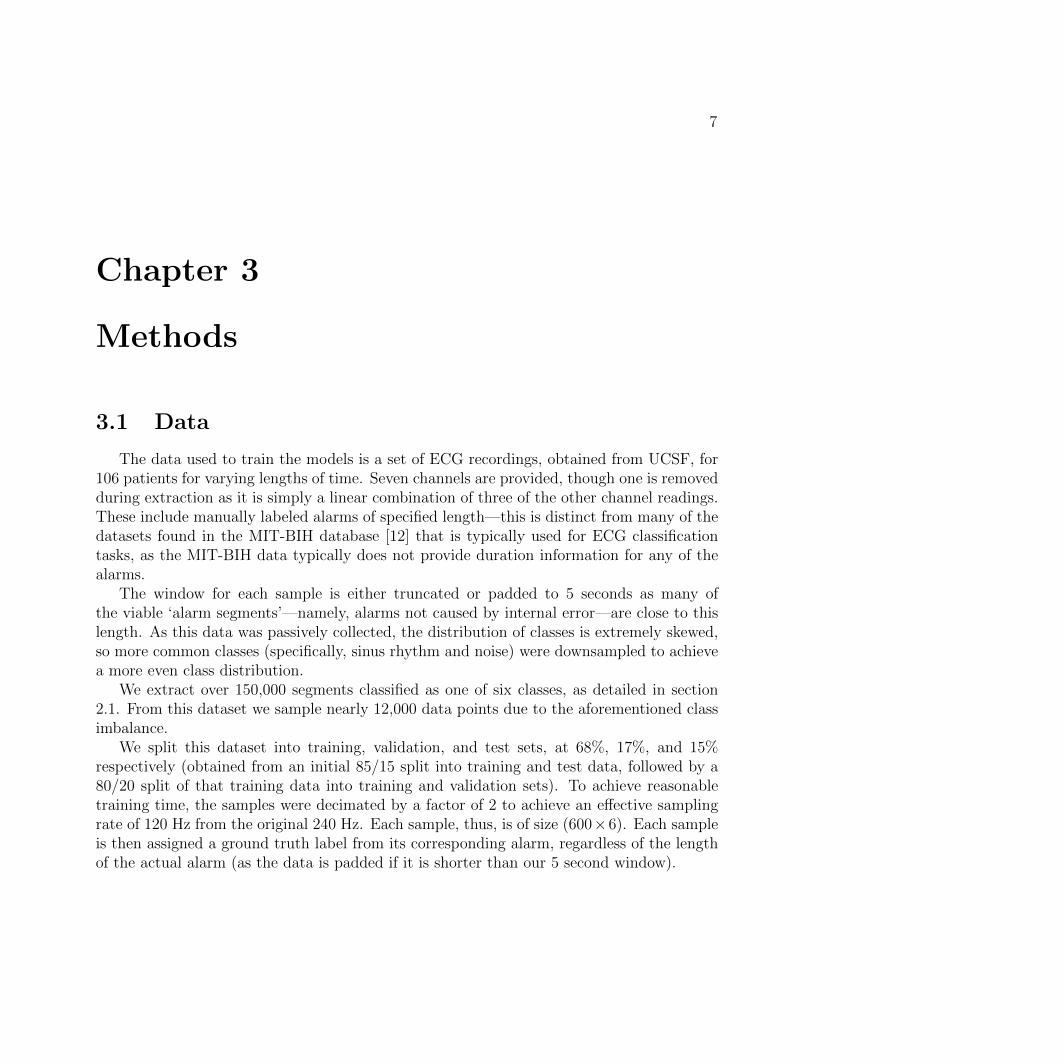
The data used to train the models is a set of ECG recordings, obtained from UCSF, for106 patients for varying lengths of time. Seven channels are provided, though one is removedduring extraction as it is simply a linear combination of three of the other channel readings.These include manually labeled alarms of specified length—this is distinct from many of thedatasets found in the MIT-BIH database [12] that is typically used for ECG classificationtasks, as the MIT-BIH data typically does not provide duration information for any of thealarms.

The window for each sample is either truncated or padded to 5 seconds as many ofthe viable ‘alarm segments’—namely, alarms not caused by internal error—are close to thislength. As this data was passively collected, the distribution of classes is extremely skewed,so more common classes (specifically, sinus rhythm and noise) were downsampled to achievea more even class distribution.

We extract over 150,000 segments classified as one of six classes, as detailed in section2.1. From this dataset we sample nearly 12,000 data points due to the aforementioned classimbalance.

We split this dataset into training, validation, and test sets, at 68%, 17%, and 15%respectively (obtained from an initial 85/15 split into training and test data, followed by a80/20 split of that training data into training and validation sets). To achieve reasonabletraining time, the samples were decimated by a factor of 2 to achieve an effective samplingrate of 120 Hz from the original 240 Hz. Each sample, thus, is of size (600×6). Each sampleis then assigned a ground truth label from its corresponding alarm, regardless of the lengthof the actual alarm (as the data is padded if it is shorter than our 5 second window).

CHAPTER 3. METHODS 8

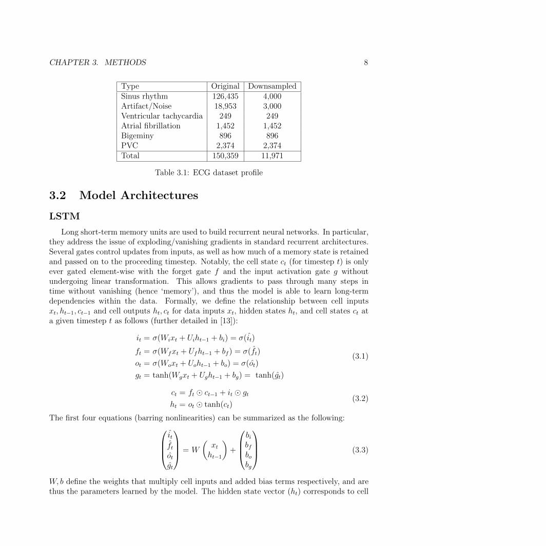
Type Original DownsampledSinus rhythm 126,435 4,000Artifact/Noise 18,953 3,000Ventricular tachycardia 249 249Atrial fibrillation 1,452 1,452Bigeminy 896 896PVC 2,374 2,374Total 150,359 11,971

Table 3.1: ECG dataset profile

3.2 Model Architectures

LSTM

Long short-term memory units are used to build recurrent neural networks. In particular,they address the issue of exploding/vanishing gradients in standard recurrent architectures.Several gates control updates from inputs, as well as how much of a memory state is retainedand passed on to the proceeding timestep. Notably, the cell state ct (for timestep t) is onlyever gated element-wise with the forget gate f and the input activation gate g withoutundergoing linear transformation. This allows gradients to pass through many steps intime without vanishing (hence ‘memory’), and thus the model is able to learn long-termdependencies within the data. Formally, we define the relationship between cell inputsxt, ht−1, ct−1 and cell outputs ht, ct for data inputs xt, hidden states ht, and cell states ct ata given timestep t as follows (further detailed in [13]):

it = σ(Wixt + Uiht−1 + bi) = σ(it)

ft = σ(Wfxt + Ufht−1 + bf ) = σ(ft)

ot = σ(Woxt + Uoht−1 + bo) = σ(ot)

gt = tanh(Wgxt + Ught−1 + bg) = tanh(gt)

(3.1)

ct = ft � ct−1 + it � gt

ht = ot � tanh(ct)(3.2)

The first four equations (barring nonlinearities) can be summarized as the following:itftotgt

= W

(xtht−1

)+

bibfbobg

(3.3)

W, b define the weights that multiply cell inputs and added bias terms respectively, and arethus the parameters learned by the model. The hidden state vector (ht) corresponds to cell


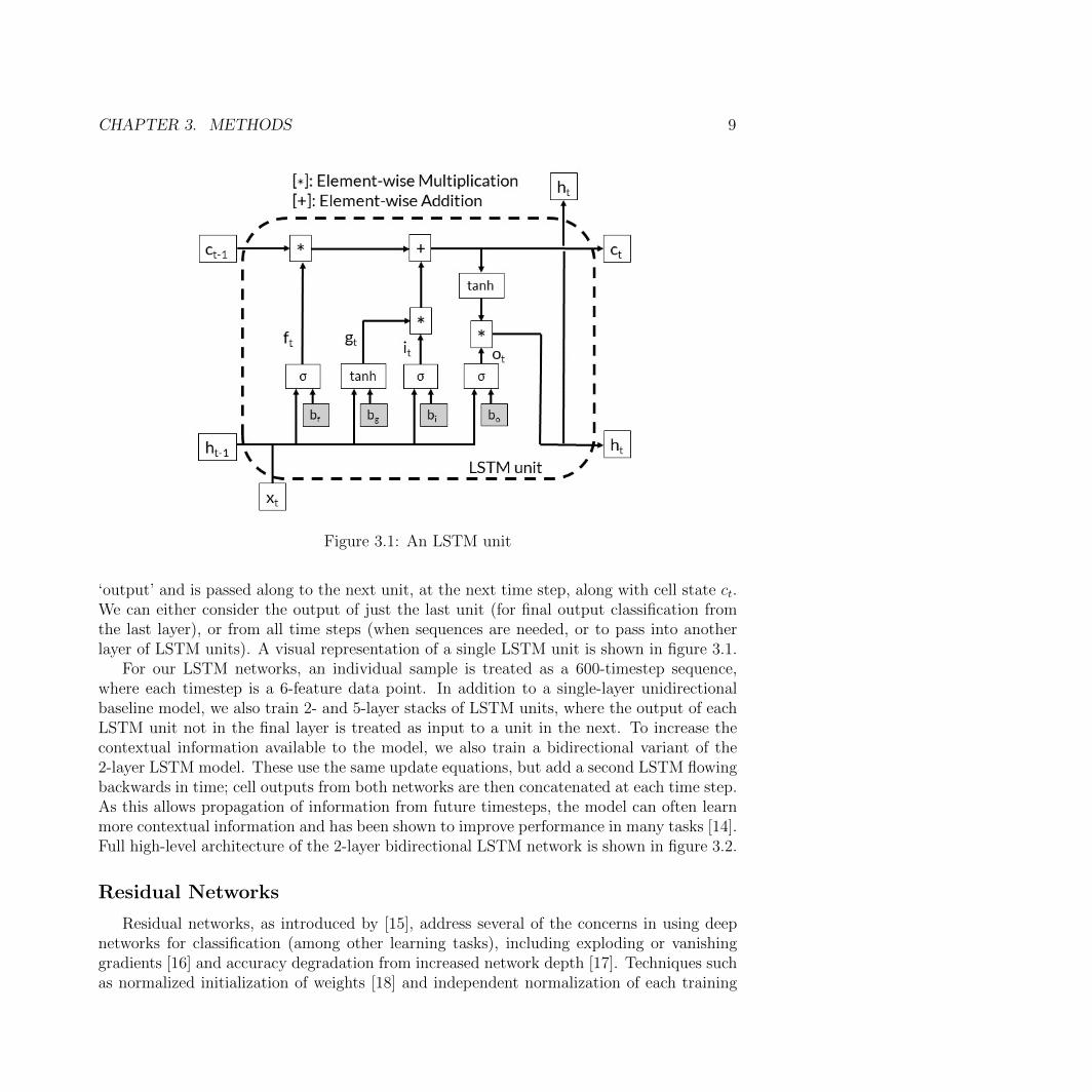
Figure 3.1: An LSTM unit

‘output’ and is passed along to the next unit, at the next time step, along with cell state ct.We can either consider the output of just the last unit (for final output classification fromthe last layer), or from all time steps (when sequences are needed, or to pass into anotherlayer of LSTM units). A visual representation of a single LSTM unit is shown in figure 3.1.

For our LSTM networks, an individual sample is treated as a 600-timestep sequence,where each timestep is a 6-feature data point. In addition to a single-layer unidirectionalbaseline model, we also train 2- and 5-layer stacks of LSTM units, where the output of eachLSTM unit not in the final layer is treated as input to a unit in the next. To increase thecontextual information available to the model, we also train a bidirectional variant of the2-layer LSTM model. These use the same update equations, but add a second LSTM flowingbackwards in time; cell outputs from both networks are then concatenated at each time step.As this allows propagation of information from future timesteps, the model can often learnmore contextual information and has been shown to improve performance in many tasks [14].Full high-level architecture of the 2-layer bidirectional LSTM network is shown in figure 3.2.

Residual Networks

Residual networks, as introduced by [15], address several of the concerns in using deepnetworks for classification (among other learning tasks), including exploding or vanishinggradients [16] and accuracy degradation from increased network depth [17]. Techniques suchas normalized initialization of weights [18] and independent normalization of each training


Figure 3.2: Bidirectional LSTM network with 2 stacked layers

batch [19] have shown to be effective in allowing deep networks to converge using standardgradient descent and backpropagation.

However, the saturation (and eventual degradation) of accuracy at high depth levelsremains an issue. As it is reflected in decreased training accuracy [15], this is not a result ofoverfitting training data. By adding identity shortcuts over various blocks in the network,gradients can flow through many layers during training without vanishing. We can thus takeadvantage of the increased representational power provided by deep networks.

In the general case, we have an input x to some set of layers (for example, a block ofconvolution, max-pooling, and activation layers) and an output F (x;W ) for a set of internalparameters W . The output of a residual block, which includes this set of layers and a residualconnection, is defined to be:

y = H(x) = F (x;W ) + x (3.4)

F (x;W ) is the residual, or the difference between input x and output y, that is to be learned.Residual connections may take different forms; in this case, our residual connections aremaxpooling layers (due to reduction in size from convolutional layers).

For our baseline and deep CNN architectures, each sample is treated as set of 6 single-channel 600-timestep recordings. These subnetworks are trained in parallel before theiroutputs are concatenated and fed into the fully connected and softmax block for classificationoutput. Each subnetwork contains multiple one-dimensional convolution and maxpool layersare stacked to form the network, and we also utilize batch normalization [19] and dropout asregularization techniques. In the case of the deeper network, we add a shortcut connection


Figure 3.3: Residual network, showing only the CNN architecture

between every two convolutional layers after the first few convolutional layers to form theresidual network structure (where the residual connection itself is a maxpool layer). In total,we use 35 convolutional layers in each subnetwork. Full high-level architecture of our residualnetwork is shown in figure 3.3.

Combined Networks

To utilize both the pattern recognition afforded by deep CNNs and the temporal learningability of LSTMs, we also train an additional architecture that combines them into a singlemodel. We begin with a stacked LSTM to extract temporal structures from the data, andinstead of feeding the unrolled hidden state into another LSTM layer, we feed it as input intoa (deep) CNN to extract localized features. In the combined model, we begin by feeding the


Figure 3.4: Combined LSTM-CNN model (LSTM portion may be uni- or bidirectional)

data into a 2-layer LSTM. The output of the final LSTM layer is treated as a one-dimensionalimage of size (100 × 600), and fed into a CNN to extract localized features. We also train asimilar architecture with a bidirectional 2-layer LSTM, where the image is of size (200×600).

Full high-level architecture of our combined network is shown in figure 3.4.

3.3 Metrics

For a given classification label, we consider how well a model predicts samples to bepositive or negative cases of that label. This is broken down into four categories: TP (truepositive) for correctly labeled positive predictions, TN (true negative) for correctly labelednegative predictions, and FP (false positive) and FN (false negative) for incorrectly labeledpositive and negative predictions respectively. In addition to overall accuracy ( TP+TN

all predictions),

we also utilize the following metrics, due to their clinical and practical significance:

Recall / Sensitivity =TP

TP + FN(3.5)

Precision / Positive Predictive Value =TP

TP + FP(3.6)


Specificity =TN

TN + FP(3.7)

F1 Score =2 · Recall · Precision

Recall + Precision(3.8)

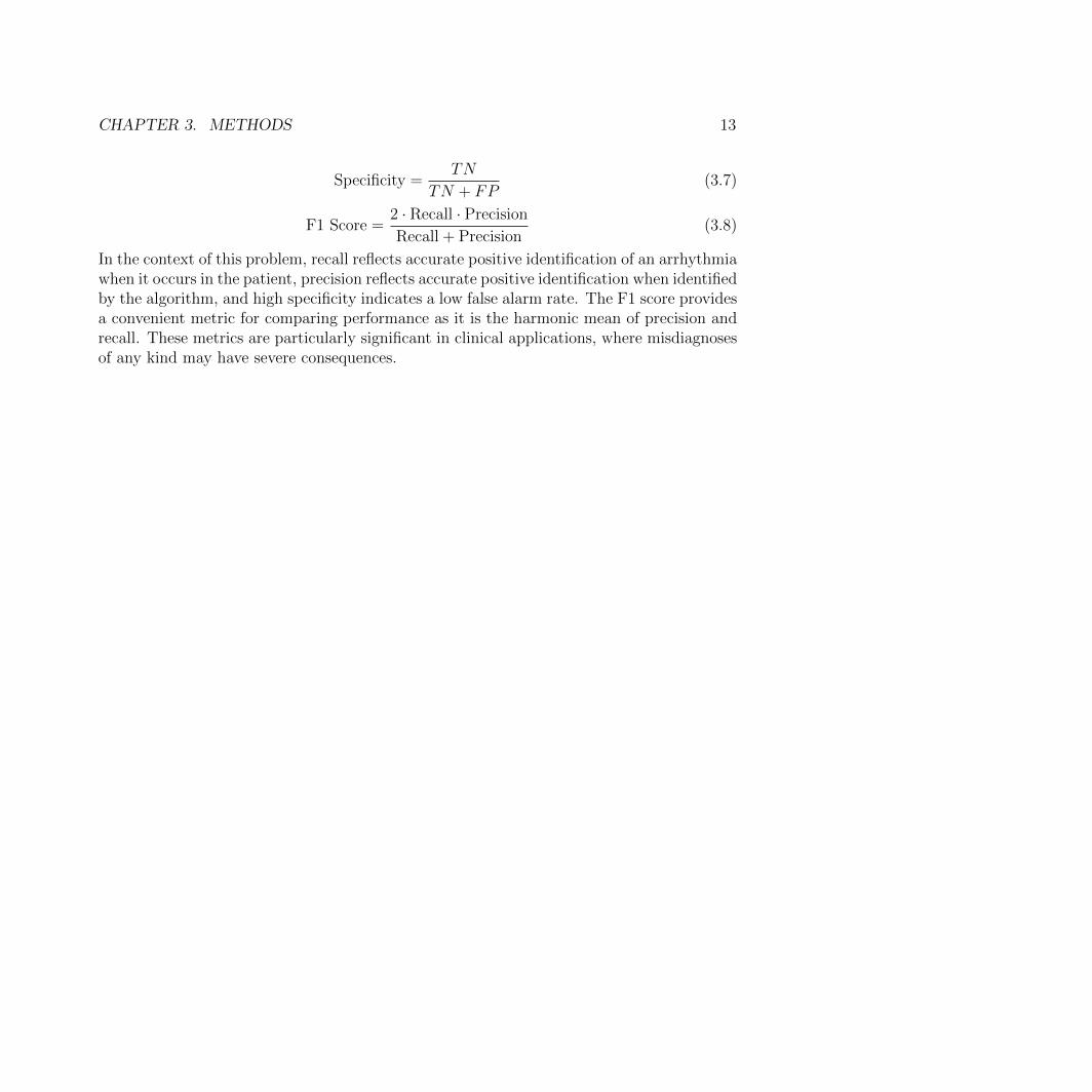
In the context of this problem, recall reflects accurate positive identification of an arrhythmiawhen it occurs in the patient, precision reflects accurate positive identification when identifiedby the algorithm, and high specificity indicates a low false alarm rate. The F1 score providesa convenient metric for comparing performance as it is the harmonic mean of precision andrecall. These metrics are particularly significant in clinical applications, where misdiagnosesof any kind may have severe consequences.

14

Chapter 4

Experiments and Results

4.1 Setup

We formulate this as a sequence classification problem, and train multiple models toinvestigate the effectiveness of a combining residual connections with LSTM architecture.We train six model architectures from three categories:

1. LSTM

• 2-layer unidirectional LSTM

• 5-layer unidirectional LSTM

• 2-layer bidirectional LSTM

2. Residual networks

• 16-block deep residual convolutional neural network

3. Combined models

• Unidirectional LSTM-CNN

• Bidirectional LSTM-CNN

Baselines

As baselines, we train a 4-block (each block containing a sequence of convolution, max-pool, batch normalization, and dropout layers) CNN with maxpool residual connections aswell as a single-layer, unidirectional LSTM with a hidden dimension of 100 (the dimension-ality of the hidden/output space as defined in section 3.2).

CHAPTER 4. EXPERIMENTS AND RESULTS 15

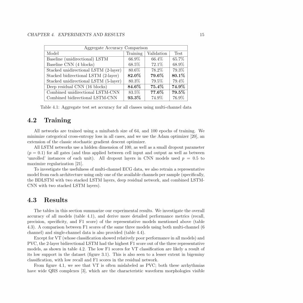
Aggregate Accuracy ComparisonModel Training Validation TestBaseline (unidirectional) LSTM 66.9% 66.4% 65.7%Baseline CNN (4 blocks) 68.5% 72.1% 68.9%Stacked unidirectional LSTM (2-layer) 80.6% 78.2% 79.3%Stacked bidirectional LSTM (2-layer) 82.0% 79.6% 80.1%Stacked unidirectional LSTM (5-layer) 80.3% 79.5% 79.4%Deep residual CNN (16 blocks) 84.6% 75.4% 74.9%Combined unidirectional LSTM-CNN 83.5% 77.6% 79.5%Combined bidirectional LSTM-CNN 93.3% 74.9% 76.9%

Table 4.1: Aggregate test set accuracy for all classes using multi-channel data

4.2 Training

All networks are trained using a minibatch size of 64, and 100 epochs of training. Weminimize categorical cross-entropy loss in all cases, and we use the Adam optimizer [20], anextension of the classic stochastic gradient descent optimizer.

All LSTM networks use a hidden dimension of 100, as well as a small dropout parameter(p = 0.1) for all gates (and thus applied between cell input and output as well as between‘unrolled’ instances of each unit). All dropout layers in CNN models used p = 0.5 tomaximize regularization [21].

To investigate the usefulness of multi-channel ECG data, we also retrain a representativemodel from each architecture using only one of the available channels per sample (specifically,the BDLSTM with two stacked LSTM layers, deep residual network, and combined LSTM-CNN with two stacked LSTM layers).

4.3 Results

The tables in this section summarize our experimental results. We investigate the overallaccuracy of all models (table 4.1), and derive more detailed performance metrics (recall,precision, specificity, and F1 score) of the representative models mentioned above (table4.3). A comparison between F1 scores of the same three models using both multi-channel (6channel) and single-channel data is also provided (table 4.4).

Except for VT (whose classification showed relatively poor performance in all models) andPVC, the 2-layer bidirectional LSTM had the highest F1 score out of the three representativemodels, as shown in table 4.2. The low F1 scores for VT classification are likely a result ofits low support in the dataset (figure 3.1). This is also seen to a lesser extent in bigeminyclassification, with low recall and F1 scores in the residual network.

From figure 4.1, we see that VT is often mislabeled as PVC; both these arrhythmiashave wide QRS complexes [3], which are the characteristic waveform morphologies visible


F1 Score Class ComparisonRhythm class BDLSTM Residual LSTM-CNNSinus rhythm 0.832 0.754 0.783Artifact/Noise 0.854 0.808 0.823Ventricular tachycardia 0.225 0.069 0.407Atrial fibrillation 0.827 0.783 0.774Bigeminy 0.683 0.116 0.543PVC 0.779 0.801 0.714Overall 0.803 0.718 0.752

Table 4.2: F1 score comparison over classes for test set, using representative LSTM (2-layerBDLSTM), residual (CNN), and combined (LSTM-CNN) models. Overall F1 score is aweighted average given the class’s support in the test set.

Classification Metrics ComparisonBDLSTM Residual LSTM-CNN

Class R P S F1 R P S F1 R P S F1S 0.83 0.84 0.95 0.83 0.89 0.65 0.87 0.75 0.78 0.79 0.94 0.78A/N 0.89 0.83 0.95 0.85 0.73 0.90 0.98 0.81 0.82 0.82 0.95 0.82VT 0.15 0.50 0.96 0.23 0.04 0.47 0.98 0.07 0.32 0.55 0.98 0.41AF 0.81 0.84 0.95 0.83 0.85 0.73 0.91 0.78 0.87 0.70 0.89 0.77B 0.71 0.66 0.83 0.68 0.06 0.90 0.99 0.12 0.46 0.66 0.98 0.54PVC 0.79 0.77 0.89 0.78 0.84 0.77 0.92 0.80 0.67 0.76 0.93 0.71

Table 4.3: Performance metric comparison over classes for test set

F1 Score Class ComparisonClass BDLSTM Residual LSTM-CNN

Multi Single Multi Single Multi SingleS 0.832 0.619 0.754 0.697 0.783 0.706A/N 0.854 0.766 0.808 0.744 0.823 0.770VT 0.234 0.021 0.069 0.075 0.407 0.143AF 0.827 0.360 0.783 0.798 0.774 0.712B 0.683 0.247 0.116 0.074 0.543 0.526PVC 0.779 0.671 0.801 0.707 0.714 0.701

Table 4.4: F1 score comparison over classes for test set, comparing single and multi-channelinput data


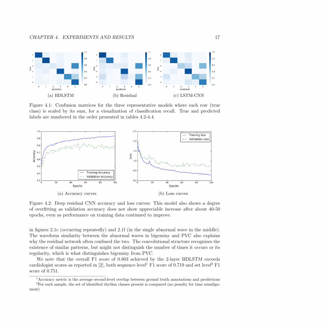
(a) BDLSTM (b) Residual (c) LSTM-CNN

Figure 4.1: Confusion matrices for the three representative models where each row (trueclass) is scaled by its sum, for a visualization of classification recall. True and predictedlabels are numbered in the order presented in tables 4.2-4.4.

(a) Accuracy curves (b) Loss curves

Figure 4.2: Deep residual CNN accuracy and loss curves: This model also shows a degreeof overfitting as validation accuracy does not show appreciable increase after about 40-50epochs, even as performance on training data continued to improve.

in figures 2.1c (occurring repeatedly) and 2.1f (in the single abnormal wave in the middle).The waveform similarity between the abnormal waves in bigeminy and PVC also explainswhy the residual network often confused the two. The convolutional structure recognizes theexistence of similar patterns, but might not distinguish the number of times it occurs or itsregularity, which is what distinguishes bigeminy from PVC.

We note that the overall F1 score of 0.803 achieved by the 2-layer BDLSTM exceedscardiologist scores as reported in [2], both sequence level1 F1 score of 0.719 and set level2 F1score of 0.751.

1Accuracy metric is the average second-level overlap between ground truth annotations and predictions2For each sample, the set of identified rhythm classes present is compared (no penalty for time misalign-

ment)


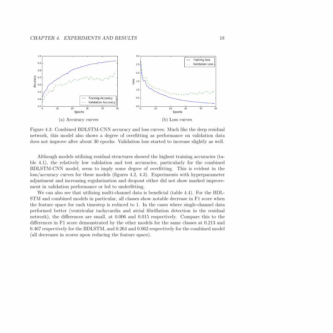
(a) Accuracy curves (b) Loss curves

Figure 4.3: Combined BDLSTM-CNN accuracy and loss curves: Much like the deep residualnetwork, this model also shows a degree of overfitting as performance on validation datadoes not improve after about 30 epochs. Validation loss started to increase slightly as well.

Although models utilizing residual structures showed the highest training accuracies (ta-ble 4.1), the relatively low validation and test accuracies, particularly for the combinedBDLSTM-CNN model, seem to imply some degree of overfitting. This is evident in theloss/accuracy curves for these models (figures 4.2, 4.3). Experiments with hyperparameteradjustment and increasing regularization and dropout either did not show marked improve-ment in validation performance or led to underfitting.

We can also see that utilizing multi-channel data is beneficial (table 4.4). For the BDL-STM and combined models in particular, all classes show notable decrease in F1 score whenthe feature space for each timestep is reduced to 1. In the cases where single-channel dataperformed better (ventricular tachycardia and atrial fibrillation detection in the residualnetwork), the differences are small, at 0.006 and 0.015 respectively. Compare this to thedifferences in F1 score demonstrated by the other models for the same classes at 0.213 and0.467 respectively for the BDLSTM, and 0.264 and 0.062 respectively for the combined model(all decreases in scores upon reducing the feature space).

19

Chapter 5

Conclusions and Future Work

We show that using known deep network algorithms for classifying time-series data allowsfor accurate classification of normal, benign, and critical arrhythmias as well as distinguishingartifacts and noise from multi-channel ECG recordings. A layered bidirectional LSTM aswell as a combined LSTM-CNN architecture is able to achieve relatively high accuracy andprecision without the use of feature engineering or extraction of previously known waveformpatterns.

We also show that ECG classification greatly benefits from the use of multi-channeldata, with nearly all classes and models showing markedly decreased accuracy when onlyone channel is used.

5.1 Limitations

An inherent limitation for this particular problem is the difficulty in obtaining accurateground truth labels. In the context of general machine learning, humans are typically theexperts from whom ground truth labels or optimal actions are learned. However, ECGclassification is inherently challenging even for practicing cardiologists; since we train themodels under the assumption that cardiologist annotations reflect the ground truth, themodels have an inherent limitation in performance.

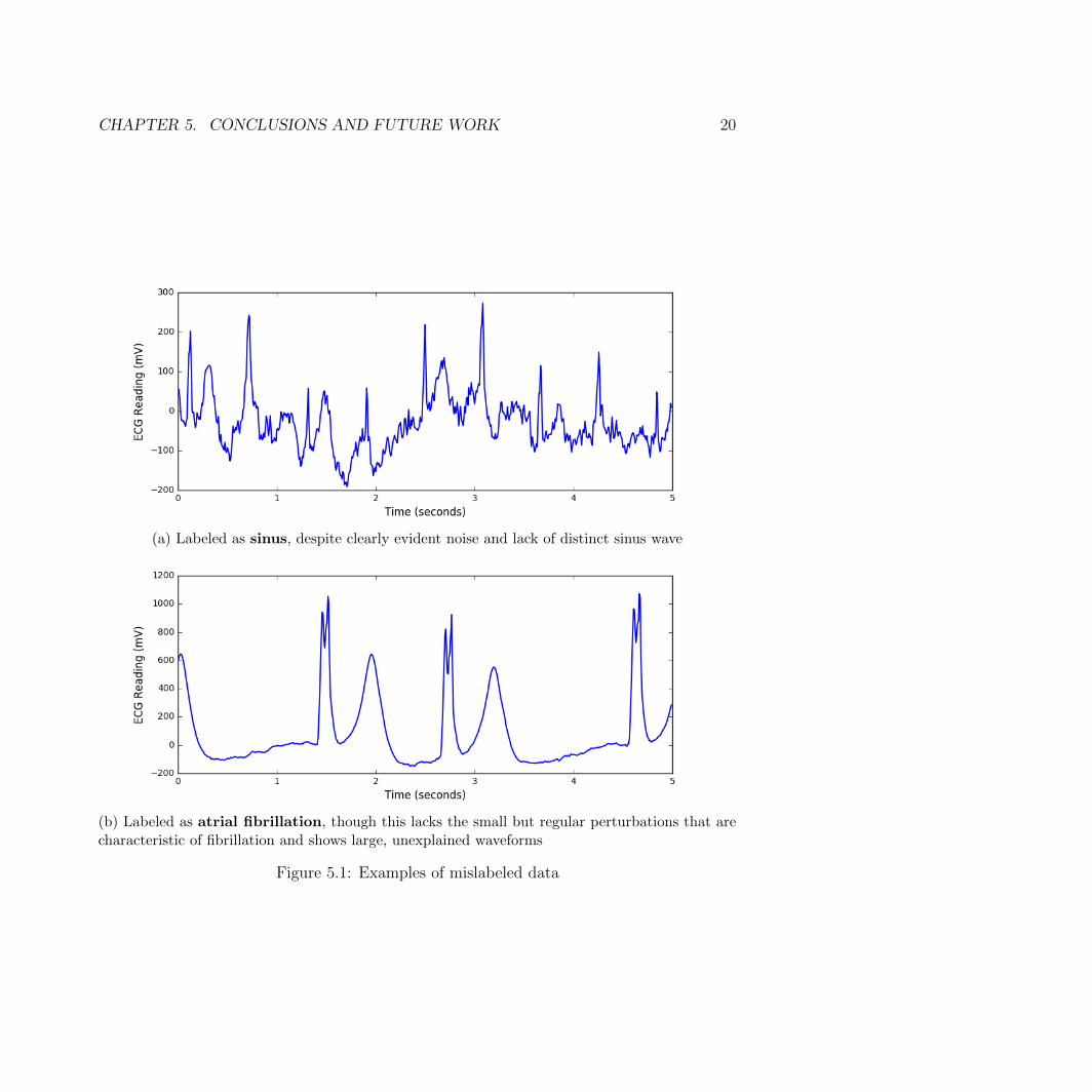
In addition, a cursory review of the data implies a small proportion of the data labelsis actually incorrect (figure 5.1). As it would be infeasible to manually check every avail-able sample, this surely introduced additional error into our model. Some arrhythmias aremorphologically very similar (figures 2.1e and 2.1f), and small differences in wave patternscan indicate different classes of arrhythmia—incorrect labels throw off the model’s learnedassumptions even further.

The low success rate of ventricular tachycardia classification is likely due to two primaryfactors: low support from the dataset, and that the few samples we do have are typicallyshort (73% of the training set examples are only 2 seconds long).

CHAPTER 5. CONCLUSIONS AND FUTURE WORK 20

(a) Labeled as sinus, despite clearly evident noise and lack of distinct sinus wave

(b) Labeled as atrial fibrillation, though this lacks the small but regular perturbations that arecharacteristic of fibrillation and shows large, unexplained waveforms

Figure 5.1: Examples of mislabeled data

CHAPTER 5. CONCLUSIONS AND FUTURE WORK 21

5.2 Future Work

Past experiments with frequency domain transformation and custom feature extraction(such as P-QRS-T wave analysis [22] and clustering [23]), have shown to be useful in iden-tifying specific arrhythmias; an ensemble model using both time series and these additionalfeatures will likely improve classification accuracy.

One area of interest is the optimization of these deeper models to perform online classi-fication on a stream of ECG data, as existing measurement devices currently perform ECGinterpretation in this way (which is necessary due to the time-critical nature of cardiac ar-rhythmia). Similarly, patient biometrics, which are typically available in real-life use casesof ECGs, can potentially be used in an integrated classifier. Patient-specific instances canbe trained on a large, diverse dataset, and fine-tuned as they receive more readings from thepatient. Underlying factors that can affect arrhythmia classification, such as resting heartrate, and existing or prior cardiac conditions, can also be incorporated.

22

References

1. Mant, J. et al. Accuracy of diagnosing atrial fibrillation on electrocardiogram by pri-mary care practitioners and interpretative diagnostic software: analysis of data fromscreening for atrial fibrillation in the elderly (SAFE) trial. BMJ 335, 380 (2007).

2. Rajpurkar, P., Hannun, A. Y., Haghpanahi, M., Bourn, C. & Ng, A. Y. Cardiologist-level arrhythmia detection with convolutional neural networks (2017).

3. ECGs for Beginners (ed de Luna, A. B.) doi:10 . 1002 / 9781118821350. <https ://doi.org/10.1002/9781118821350> (John Wiley & Sons, Ltd, Sept. 2014).

4. Drew, B. J. et al. Insights into the problem of alarm fatigue with physiologic monitordevices: a comprehensive observational study of consecutive intensive care unit patients.PloS ONE 9, e110274 (2014).

5. Bortolan, G., Degani, R. & Willems, J. L. Neural networks for ECG classification inComputers in Cardiology 1990, Proceedings. (1990), 269–272.

6. Coast, D. A., Stern, R. M., Cano, G. G. & Briller, S. A. An approach to cardiacarrhythmia analysis using hidden Markov models. IEEE Transactions on BiomedicalEngineering 37, 826–836 (1990).

7. Cheng, W. & Chan, K. Classification of electrocardiogram using hidden Markov modelsin Engineering in Medicine and Biology Society, 1998. Proceedings of the 20th AnnualInternational Conference of the IEEE (1998), 143–146.

8. Schels, H. F., Haberl, R., Jilge, G., Steinbigler, P. & Steinbeck, G. Frequency analysisof the electrocardiogram with maximum entropy method for identification of patientswith sustained ventricular tachycardia. IEEE Transactions on Biomedical Engineering38, 821–826 (1991).

9. Afonso, V. X. & Tompkins, W. J. Detecting ventricular fibrillation. IEEE Engineeringin Medicine and Biology Magazine 14, 152–159 (1995).

10. Zheng, Y., Liu, Q., Chen, E., Ge, Y. & Zhao, J. L. Exploiting multi-channels deepconvolutional neural networks for multivariate time series classification. Frontiers ofComputer Science 10, 96–112 (2016).

11. Yang, J., Nguyen, M. N., San, P. P., Li, X. & Krishnaswamy, S. Deep ConvolutionalNeural Networks on Multichannel Time Series for Human Activity Recognition. in IJ-CAI (2015), 3995–4001.

REFERENCES 23

12. Goldberger, A. L. et al. PhysioBank, PhysioToolkit, and PhysioNet: Components of aNew Research Resource for Complex Physiologic Signals. Circulation 101, e215–e220(2000 (June 13)).

13. Hochreiter, S. & Schmidhuber, J. Long short-term memory. Neural Computation 9,1735–1780 (1997).

14. Cui, Z., Ke, R. & Wang, Y. Deep Bidirectional and Unidirectional LSTM RecurrentNeural Network for Network-wide Traffic Speed Prediction (2018).

15. He, K., Zhang, X., Ren, S. & Sun, J. Deep residual learning for image recognition inProceedings of the IEEE conference on computer vision and pattern recognition (2016),770–778.

16. Bengio, Y., Simard, P. & Frasconi, P. Learning long-term dependencies with gradientdescent is difficult. IEEE Transactions on Neural Networks 5, 157–166 (1994).

17. He, K. & Sun, J. Convolutional neural networks at constrained time cost in 2015 IEEEConference on Computer Vision and Pattern Recognition (CVPR) (2015), 5353–5360.

18. He, K., Zhang, X., Ren, S. & Sun, J. Delving deep into rectifiers: Surpassing human-level performance on imagenet classification in Proceedings of the IEEE InternationalConference on Computer Vision (2015), 1026–1034.

19. Ioffe, S. & Szegedy, C. Batch normalization: Accelerating deep network training byreducing internal covariate shift (2015).

20. Kingma, D. P. & Ba, J. Adam: A method for stochastic optimization (2014).

21. Baldi, P. & Sadowski, P. J. Understanding dropout in Advances in Neural InformationProcessing Systems (2013), 2814–2822.

22. Karpagachelvi, S., Arthanari, M. & Sivakumar, M. ECG feature extraction techniques-asurvey approach (2010).

23. Ye, C., Kumar, B. V. & Coimbra, M. T. Heartbeat classification using morphologicaland dynamic features of ECG signals. IEEE Transactions on Biomedical Engineering59, 2930–2941 (2012).

arrhythmia classification in multi-channel ecg signals ...using a dataset of 106 patient readings,...

Documents