Artificial Neural Networks (ANN)

Patricia J Riddle Computer Science 760

8/21/15 1 ANN

Artificial Neural Networks

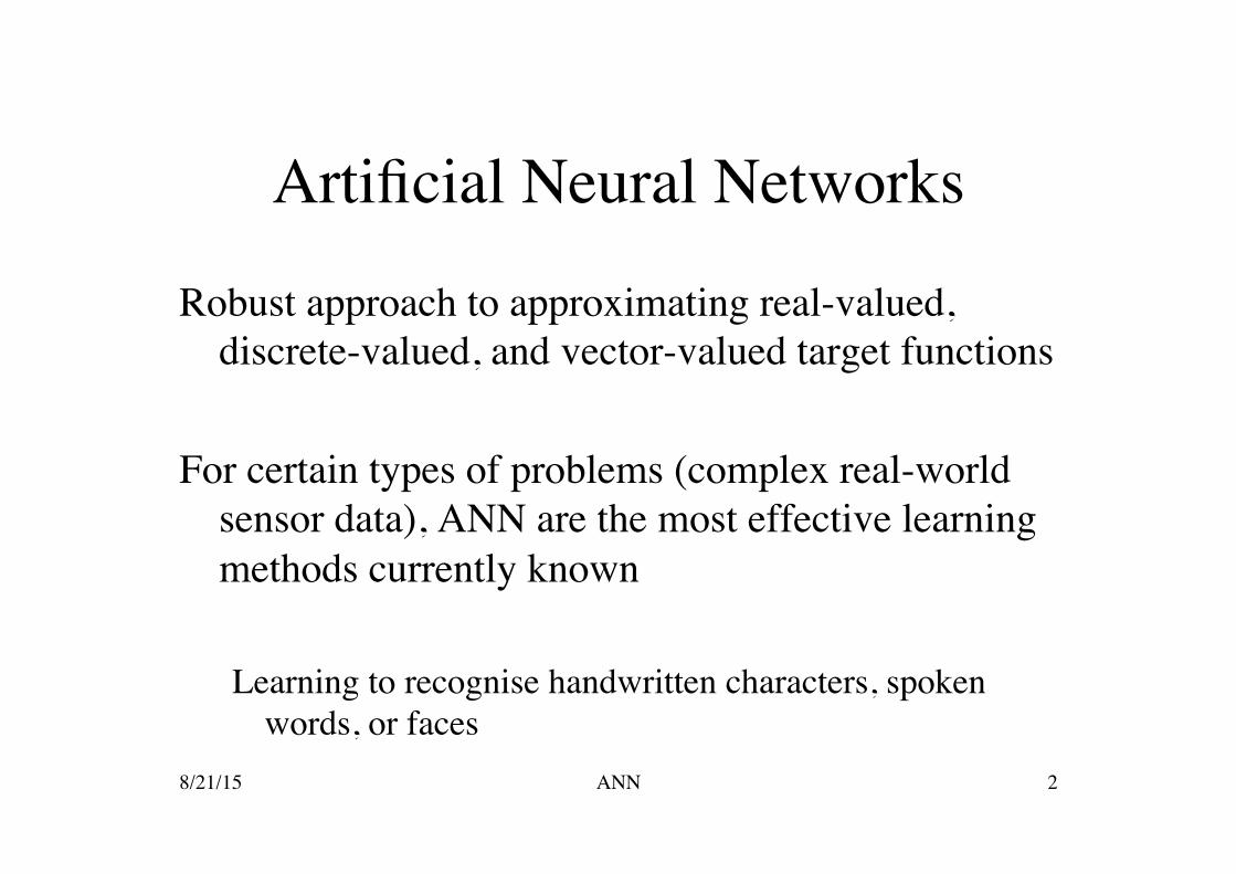
Robust approach to approximating real-valued, discrete-valued, and vector-valued target functions

For certain types of problems (complex real-world

sensor data), ANN are the most effective learning methods currently known

Learning to recognise handwritten characters, spoken

words, or faces 8/21/15 2 ANN

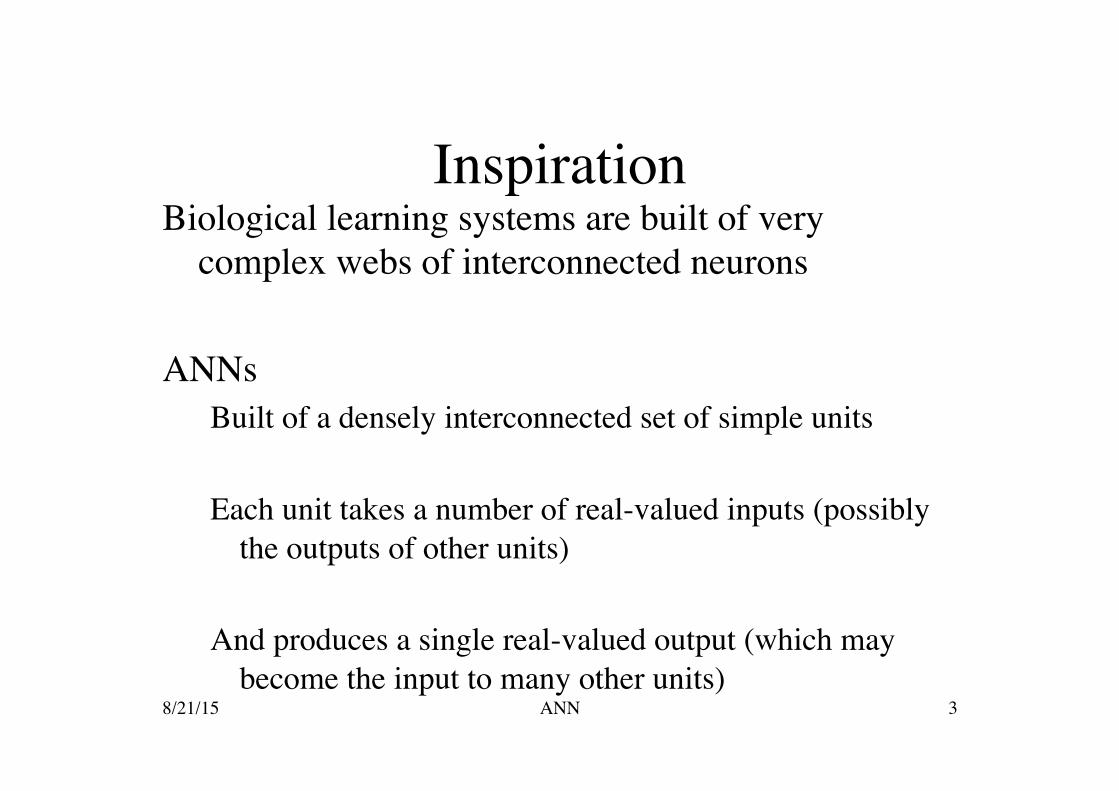
Inspiration Biological learning systems are built of very

complex webs of interconnected neurons ANNs

Built of a densely interconnected set of simple units Each unit takes a number of real-valued inputs (possibly

the outputs of other units) And produces a single real-valued output (which may

become the input to many other units) 8/21/15 3 ANN

Human Brain 1011 densely interconnected neurons Each neuron connected to 104 others Switching time:

Human 10-3 seconds Computer 10-4 seconds

10-1 seconds to visually recognise your mother So only a few hundred steps Must be highly parallel computation based on distributed

representations 8/21/15 4 ANN

Researchers

Two Groups of Researchers: Use ANN to study and model biological learning

processes Obtaining highly effective machine learning

algorithms

8/21/15 5 ANN

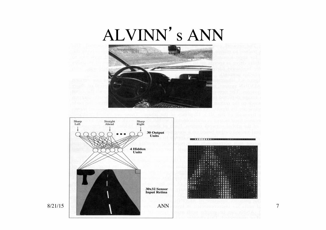
Neural Network Representations ALVINN - ANN to steer an autonomous vehicle

driving at normal speeds on public highways Input - 30 x 32 grid of pixel intensities from a

forward-pointed camera Output - direction vehicle is steered Trained to mimic the observed steering commands of

a human driving the vehicle for 5 minutes 8/21/15 6 ANN

ALVINN’s ANN

8/21/15 7 ANN

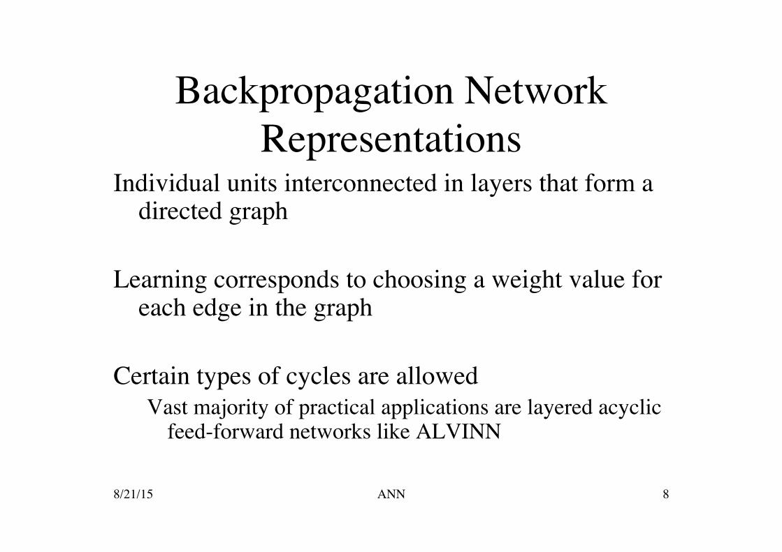
Backpropagation Network Representations

Individual units interconnected in layers that form a directed graph

Learning corresponds to choosing a weight value for

each edge in the graph Certain types of cycles are allowed

Vast majority of practical applications are layered acyclic feed-forward networks like ALVINN

8/21/15 8 ANN

Appropriate Problems for ANN

Training data is noisy, complex sensor data Also problems where symbolic algorithms are

used - decision tree learning (DTL) ANN and DTL produce results of comparable

accuracy

8/21/15 9 ANN

Specifically Instances are attribute-value pairs

attributes may be highly correlated or independent, values can be any real value

Target function may be discrete-valued, real-valued or vector-valued

8/21/15 10 ANN

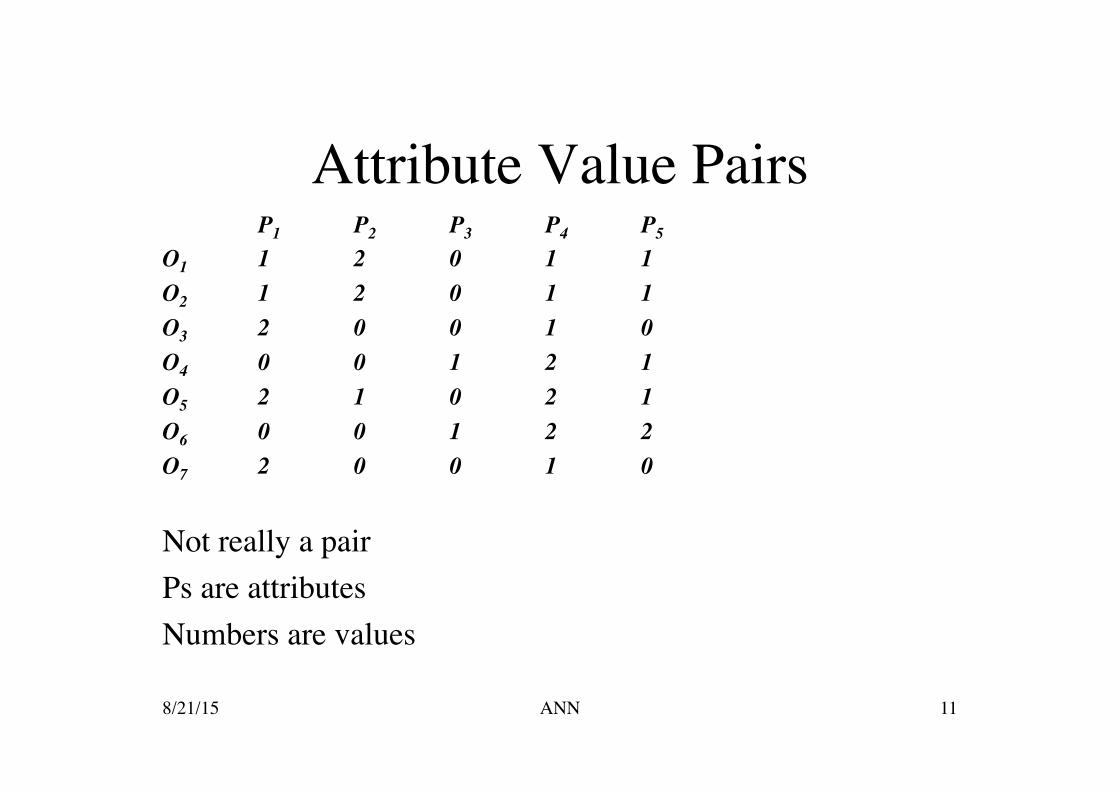
Attribute Value Pairs P1 P2 P3 P4 P5

O1 1 2 0 1 1 O2 1 2 0 1 1 O3 2 0 0 1 0 O4 0 0 1 2 1 O5 2 1 0 2 1 O6 0 0 1 2 2 O7 2 0 0 1 0

Not really a pair Ps are attributes Numbers are values

8/21/15 ANN 11

More Specifically Training examples may contain errors Long training times are acceptable Can Require fast evaluation of the learned target

function Humans do NOT need to understand the learned

target function!!! 8/21/15 12 ANN

ANN Solution

[ 2.8 3.4 1.6 1.2 0.6 3.2 4.5 1.3 0.8 ]

8/21/15 ANN 13

Perceptrons Inputs a vector of real-valued inputs

calculates a linear combination and outputs a 1 if the result is greater than some threshold and

-1 otherwise Hyperplane decision surface in the n-dimensional

space of instances Not all datasets can be separated by a hyperplane,

but if they can they are linearly separable datasets 8/21/15 14 ANN

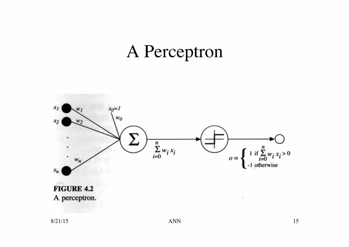
A Perceptron

8/21/15 15 ANN

Linearly Separable

8/21/15 16 ANN

Even More Specifically

Each wi is a real-valued weight that determines the contribution of the input xi to the perceptron output

The quantity (-w0) is the threshold

€

o(x1,..,xn ) =1 if w0 +w1x1+w2x2 + ...+wnxn >0= −1 otherwise

8/21/15 17 ANN

Threshold Explained

Remember algebra????

8/21/15 ANN 18

€

w0 +w1x1+w2x2 + ...+wnxn > 0

w1x1+w2x2 + ...+wnxn > 0 − w0

w1x1+w2x2 + ...+wnxn > − w0

A Perceptron

8/21/15 19 ANN

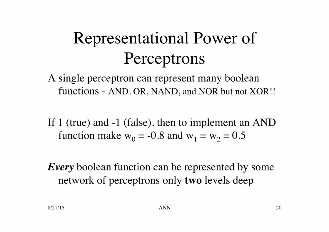
Representational Power of Perceptrons

A single perceptron can represent many boolean functions - AND, OR, NAND, and NOR but not XOR!!

If 1 (true) and -1 (false), then to implement an AND

function make w0 = -0.8 and w1 = w2 = 0.5 Every boolean function can be represented by some

network of perceptrons only two levels deep

8/21/15 20 ANN

Perceptron Learning Algorithms Determine a weight vector that produces the correct

±1 output for each of the training examples Several algorithms are known to solve this problem:

–  The perceptron rule –  The delta rule

Guaranteed to converge to somewhat different acceptable hypothesis under somewhat different conditions

These are the basis for learning networks of many units - ANNs

8/21/15 21 ANN

The perceptron rule

8/21/15 ANN 22

Basis of Perceptron Training Rule

Begin with random weights modify them repeat until the perceptron classifies all training

examples correctly

8/21/15 23 ANN

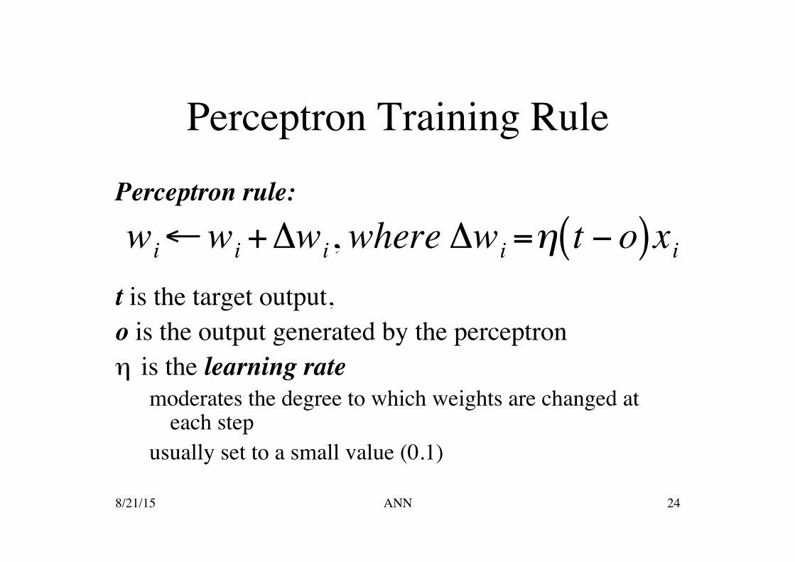
Perceptron Training Rule Perceptron rule: t is the target output, o is the output generated by the perceptron η  is the learning rate

moderates the degree to which weights are changed at each step

usually set to a small value (0.1)

€

wi←wi +Δwi, where Δwi =η t − o( )xi

8/21/15 24 ANN

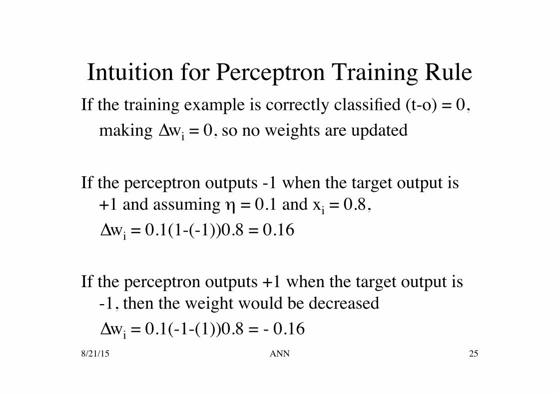
Intuition for Perceptron Training Rule If the training example is correctly classified (t-o) = 0, making ∆wi = 0, so no weights are updated

If the perceptron outputs -1 when the target output is

+1 and assuming η = 0.1 and xi = 0.8, ∆wi = 0.1(1-(-1))0.8 = 0.16

If the perceptron outputs +1 when the target output is -1, then the weight would be decreased ∆wi = 0.1(-1-(1))0.8 = - 0.16

8/21/15 25 ANN

Convergence of Perceptron Training Rule

This learning procedure will converge within finite number of applications of the perceptron training rule to a weight vector that correctly classifies all training examples,

provided

1.  the training examples are linearly separable and 2.  a sufficiently small learning rate, η, is used.

8/21/15 26 ANN

The delta rule

8/21/15 ANN 27

Gradient Descent Algorithm

If training examples are not linearly separable, the delta rule converges toward best-fit

approximation Use gradient descent to find the weights that best

fit the training examples basis of the Backpropagation Algorithm

8/21/15 28 ANN

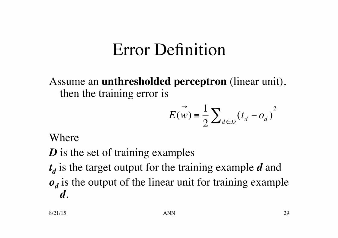
Error Definition Assume an unthresholded perceptron (linear unit),

then the training error is Where D is the set of training examples td is the target output for the training example d and od is the output of the linear unit for training example

d.

€

E(w→

) ≡ 12

(td − od )d ∈D∑2

8/21/15 29 ANN

Perceptron vs Linear Unit

8/21/15 30 ANN

Error Surface

Given the above error definition, the error surface must be parabolic with a single

global minimum.

8/21/15 31 ANN

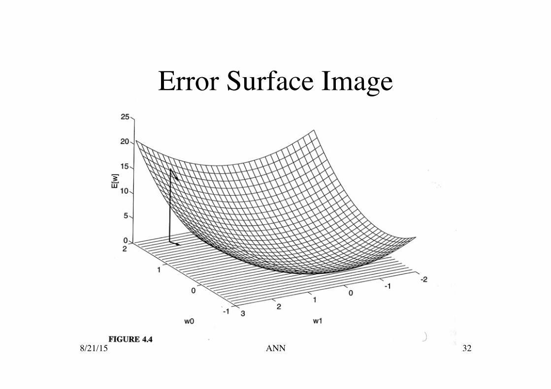
Error Surface Image

8/21/15 32 ANN

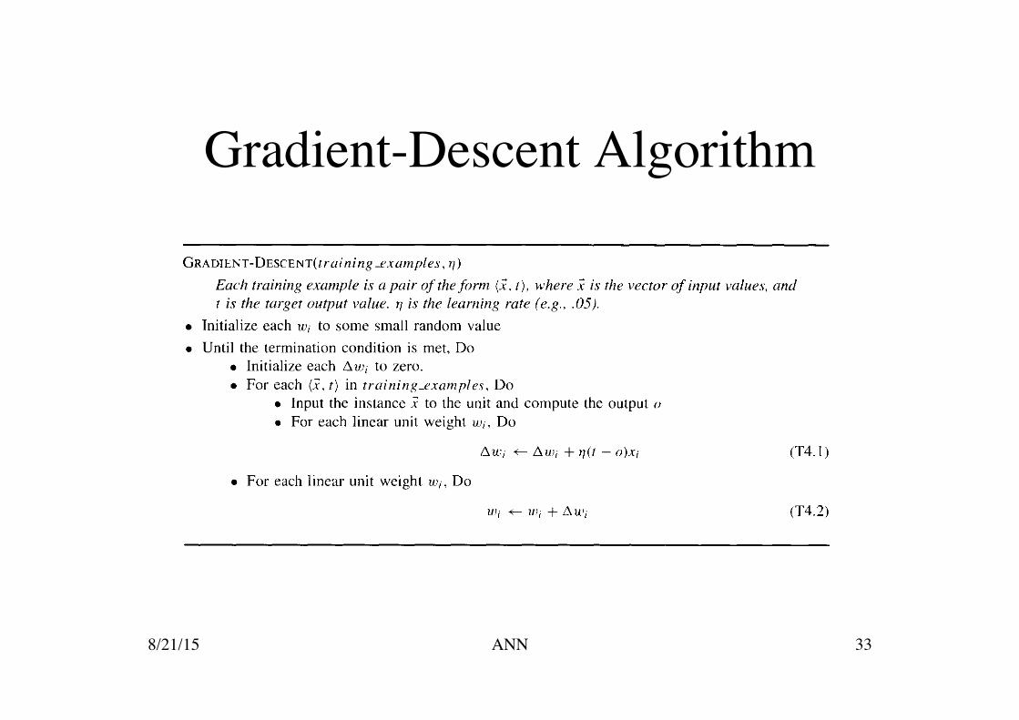
Gradient-Descent Algorithm

8/21/15 33 ANN

Weight Update Rule Intuition Gradient descent determines the weight vector that

minimizes E. It starts with an arbitrary weight vector, modifies it in small steps in the direction that produces the steepest descent, and continues until the global minimum error is reached,

8/21/15 34 ANN

Weight Update Rule

Weight update rule: Where xid denotes input component xi for training example d €

Δwi =η (td − od )d ∈D∑ xid

8/21/15 35 ANN

Convergence Because the error surface contains only a single global minimum, the algorithm will converge to a weight vector with minimum

error, regardless of whether the training examples are linearly

separable, given a sufficiently small learning rate η is used. Hence a common modification is to gradually reduce the value of

η as the number of steps grows. 8/21/15 36 ANN

Gradient descent ���Important General Paradigm

When Continuously parameterized hypothesis i.e., The error can be differentiated with

respect to the hypothesis parameters

8/21/15 37 ANN

Problems with Gradient descent 1.  Converging to a local minimum can be

quite slow

2.  If there are multiple local minima, then there is no guarantee that the procedure will find the global minimum

–  The error surface will not be parabolic with a single global minima, when training multiple nodes.

8/21/15 38 ANN

Stochastic Gradient Descent Approximate gradient descent search by updating weights

incrementally, following the calculation of the error for each individual example

Delta rule: (same as LMS algorithm in 367, but only similar to

perceptron training rule because using linear unit) €

Δwi =η(t − o)xi

8/21/15 39 ANN

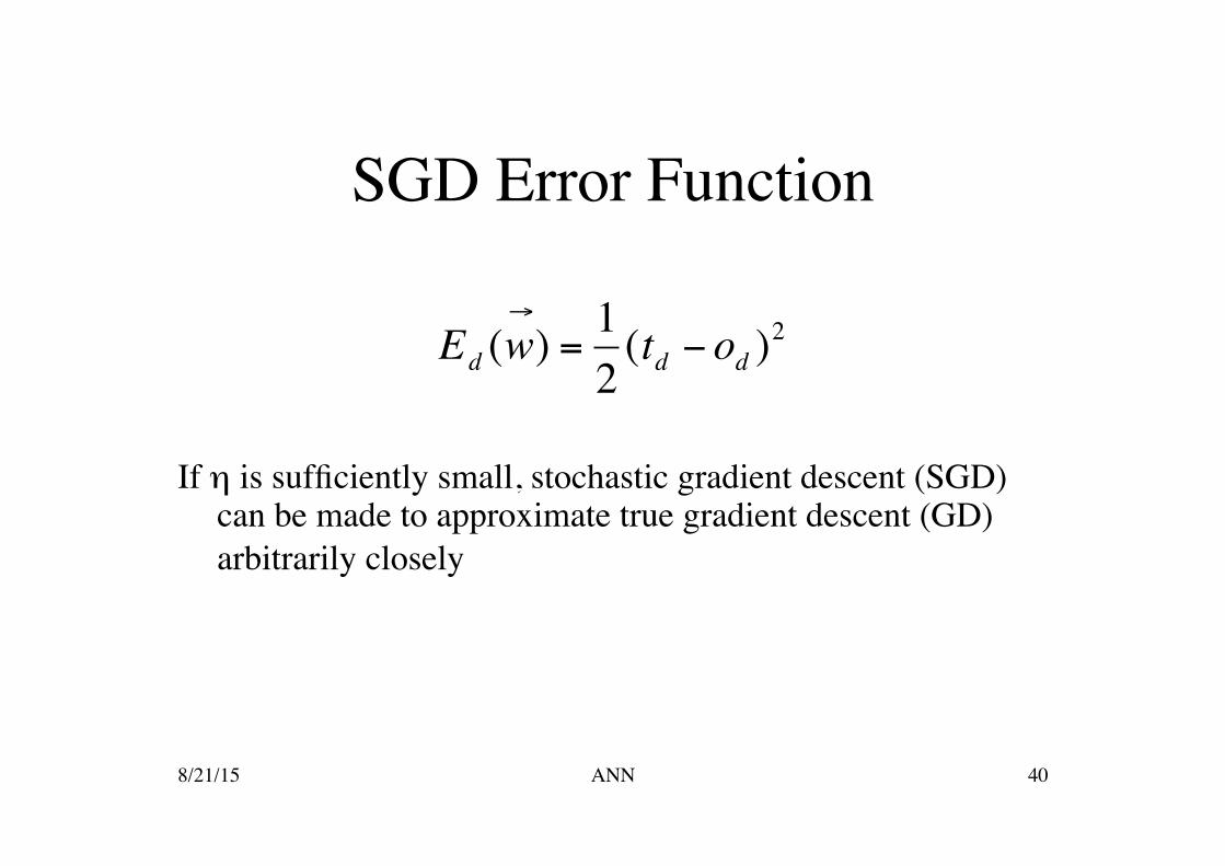
SGD Error Function If η is sufficiently small, stochastic gradient descent (SGD)

can be made to approximate true gradient descent (GD) arbitrarily closely €

Ed (w→

) =12(td − od )

2

8/21/15 40 ANN

Difference between GD and SGD In GD the error is summed over all examples before

updating weights In SGD weights are updated upon examining each training

example Summing over multiple examples in GD requires more

computation per weight update step. But since it uses the True gradient, it is often used with a larger step size (larger η).

If there are multiple local minima with respect to the error

function, SGD can sometimes avoid falling into these local minima.

8/21/15 41 ANN

Difference between Delta Rule &���Perceptron Training Rule

Appear identical, but

PTR is for thresholded perceptron and DR is for a linear unit (or unthresholded

perceptron).

8/21/15 42 ANN

Perceptron vs Linear Unit

8/21/15 43 ANN

Delta Rule with Thresholded perceptron

If the unthresholded perceptron can be trained to fit these values perfectly then so can the thresholded perceptron.

DR can be used to train a thresholded perceptron, by using

±1 as target values to a linear unit and having the thresholded unit return the sign of the linear unit.

If the target values cannot be perfectly fit, then the

thresholded perceptron will be correct whenever the linear unit has the right sign, but this is not guaranteed to happen

8/21/15 44 ANN

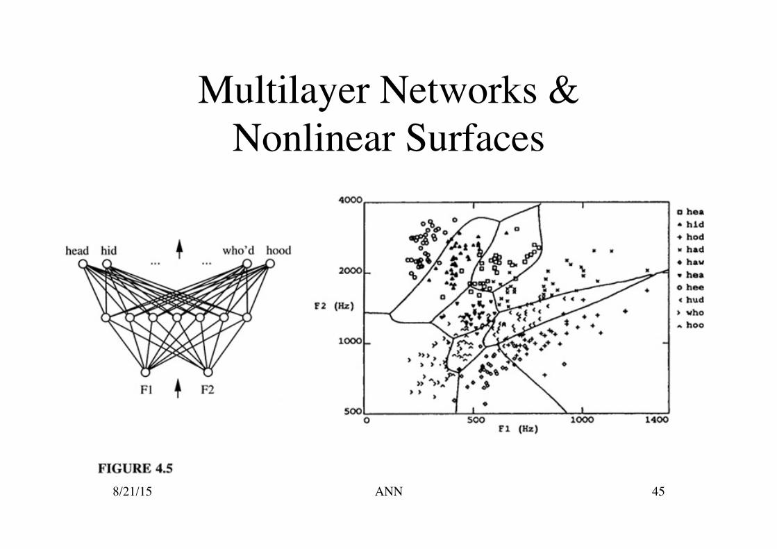
Multilayer Networks & Nonlinear Surfaces

8/21/15 45 ANN

Multilayer Networks Multiple layers of linear units still produce only linear

functions!!! Perceptrons have a discontinuous threshold which is

undifferentiable and therefore unsuitable for gradient descent

We want a unit whose output is a nonlinear differentiable

function of the inputs One solution is a sigmoid unit 8/21/15 46 ANN

What is a Sigmoid Unit?

Like perceptrons it computes a linear combination of its inputs

and then applies a threshold to the result. But the threshold output is a continuous

function of its input which ranges from 0 to 1. If is often referred to as a squashing function.

8/21/15 47 ANN

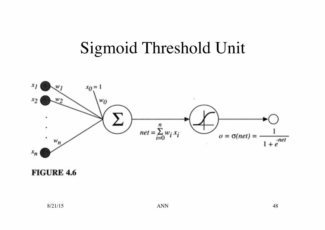
Sigmoid Threshold Unit

8/21/15 48 ANN

Properties of the Backpropagation Algorithm

Learns weights for a multilayer network, given a fixed set of units and interconnections

It uses gradient descent to minimize the

squashed error between the network outputs and the target values for these outputs

8/21/15 49 ANN

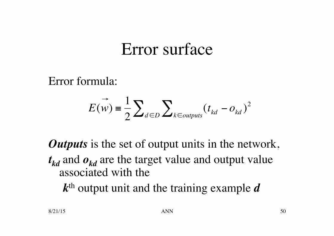
Error surface

Error formula: Outputs is the set of output units in the network, tkd and okd are the target value and output value

associated with the kth output unit and the training example d

€

E(w→

) ≡ 12

(tkd − okd )2

k∈outputs∑d ∈D∑

8/21/15 50 ANN

Error Surface

In multilayer networks the error surface can have multiple minima,

In practice Backpropagation has produced excellent results in many real-world applications.

The algorithm (on the next page) is for two

layers of sigmoid units and does stochastic gradient descent.

8/21/15 51 ANN

Backpropagation Algorithm

8/21/15 52 ANN

Backpropogation Weight Training Rule���Output Units

δkß ok(1-ok)(tk-ok) The error (t-o) in the delta rule is replaced by δj. The output unit k is the familiar (tk -ok) from the delta rule

multiplied by ok(1-ok) ok(1-ok) is the derivative of the sigmoid squashing function. 8/21/15 53 ANN

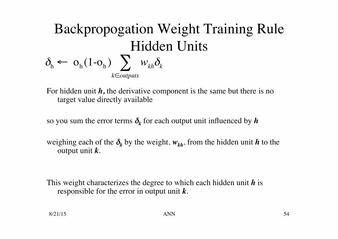
Backpropogation Weight Training Rule���Hidden Units

For hidden unit h, the derivative component is the same but there is no

target value directly available so you sum the error terms δk for each output unit influenced by h weighing each of the δk by the weight, wkh, from the hidden unit h to the

output unit k. This weight characterizes the degree to which each hidden unit h is

responsible for the error in output unit k. 8/21/15 54 ANN

δh ← oh (1-oh ) wkhk∈outputs∑ δk

Multilayer Networks & Nonlinear Surfaces

8/21/15 55 ANN

Termination Conditions for Backpropagation

Halt after a fixed number of iterations. Halt once the error on the training examples falls below some

threshold. Halt once the error on a separate validation set of examples

meets some criterion. Important:

Too few iterations - fail to reduce error sufficiently Too many iterations - overfit the data - 367

8/21/15 56 ANN

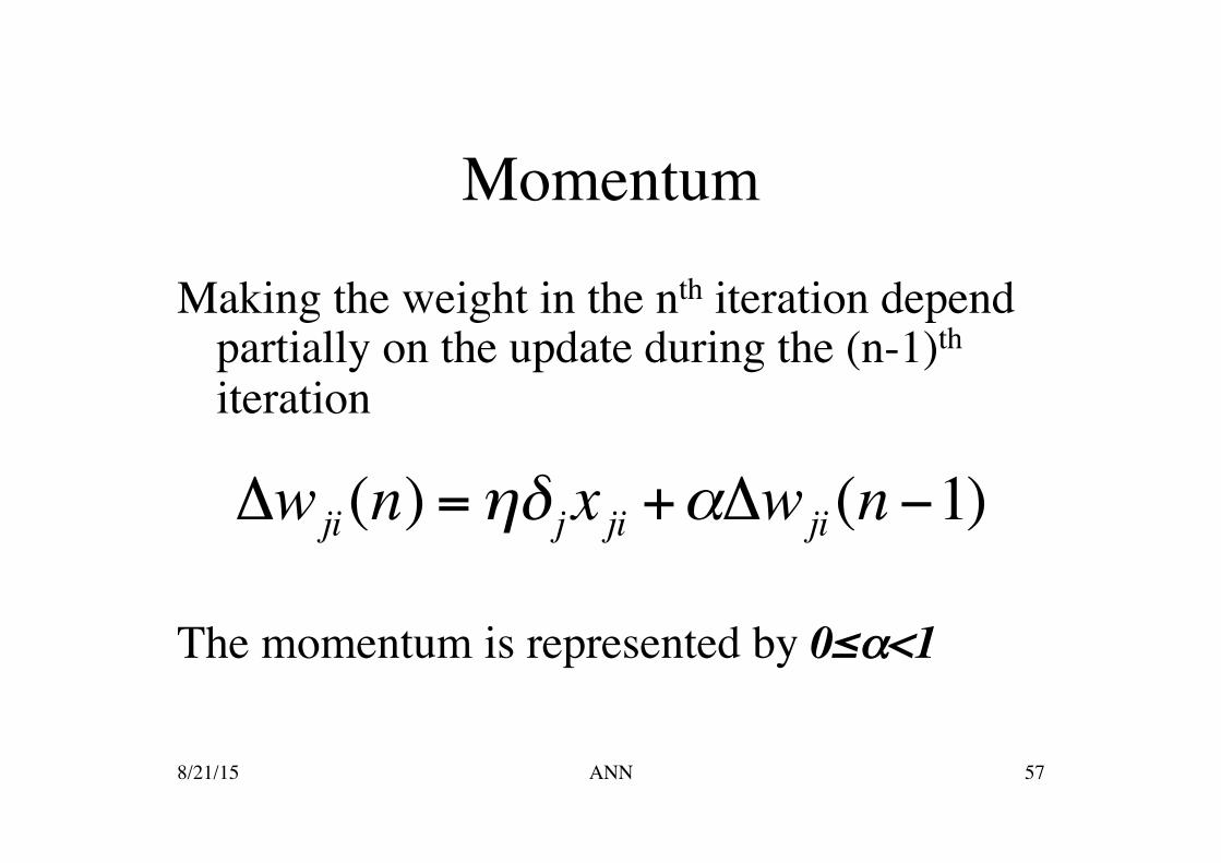
Momentum

Making the weight in the nth iteration depend partially on the update during the (n-1)th iteration

The momentum is represented by 0≤α<1

Δwji (n) =ηδ j x ji +αΔwji (n−1)

8/21/15 57 ANN

Intuition behind Momentum The gradient search trajectory is analogous to a

momentumless ball rolling down the error surface, the effect of α is to keep the ball rolling in the same direction from one iteration to the next.

The ball can roll through small local minima or along flat

regions in the surface where the ball would stop without momentum.

It also causes a gradual increase in the step size in regions

where the gradient is unchanging, thereby speeding convergence.

8/21/15 58 ANN

Arbitrary Acyclic Networks Only equation (T4.4) has to change Feedforward networks of arbitrary depth Directed acyclic graph, not arranged in uniform layers

€

δr = or (1− or ) wsrδss∈layer m+1∑

€

δr = or (1− or ) wsrδss∈Downstream(r)∑

8/21/15 59 ANN

Convergence and Local Minima

The error surface in multilayer neural networks may contain many different local minima where gradient descent can become trapped.

But backpropagation is a highly effective function

approximation in practice. Why??

8/21/15 60 ANN

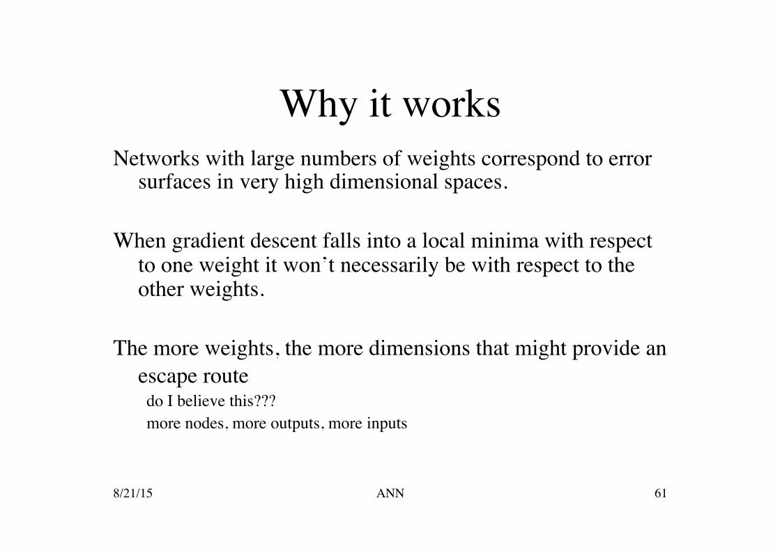
Why it works Networks with large numbers of weights correspond to error

surfaces in very high dimensional spaces. When gradient descent falls into a local minima with respect

to one weight it won’t necessarily be with respect to the other weights.

The more weights, the more dimensions that might provide an

escape route do I believe this??? more nodes, more outputs, more inputs

8/21/15 61 ANN

Heuristics to Overcome Local Minima Add momentum Use stochastic gradient search New seed (e.g., initial random weights), and choose

the one with the best performance on the validation set or treat as a committee or ensemble Is this cheating??

Add more dimensions (within reason) 8/21/15 62 ANN

Representational Power of Feedforward Networks

Boolean functions: 2 layers of units, but number of hidden nodes grows exponentially in the number of inputs.

Continuous Functions: every bounded continuous

function to arbitrary accuracy in 2 layers of units. Arbitrary functions: arbitrary accuracy by a network

with 3 layers of units - based on linear combination of many localized functions.

8/21/15 63 ANN

Caveats

Arbitrary error??? “Warning Will Robinson”

Network weight variables reachable from the

initial weight values may not include all possible weight vectors!!!!!

8/21/15 64 ANN

Hypothesis Space Every possible assignment of network weights

represents a syntactically different hypothesis. N-dimensional Euclidean space of the n network

weights. This hypothesis space is continuous. Since E is differentiable with respect to the

continuous parameters, we have a well-defined error gradient

8/21/15 65 ANN

Inductive Bias Inductive Bias depends on interplay between

gradient descent search and the way the weight space spans the space of representable functions.

Roughly - smooth interpolation between data points Given two positive training instances with no

negatives between them, Backpropagation will tend to label the points between as positive.

8/21/15 66 ANN

Hidden Layer Representations

Backpropagation can discover useful intermediate representations at the hidden unit layers.

It is a way to make implicit concepts explicit. Discovering binary encoding

8/21/15 67 ANN

Mutilated Chessboard problem

8/21/15 68 ANN

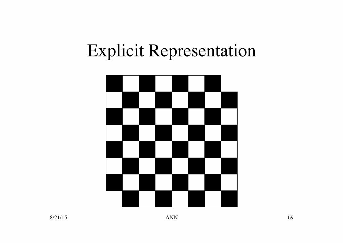
Explicit Representation

8/21/15 69 ANN

Backprop in action

8/21/15 70 ANN

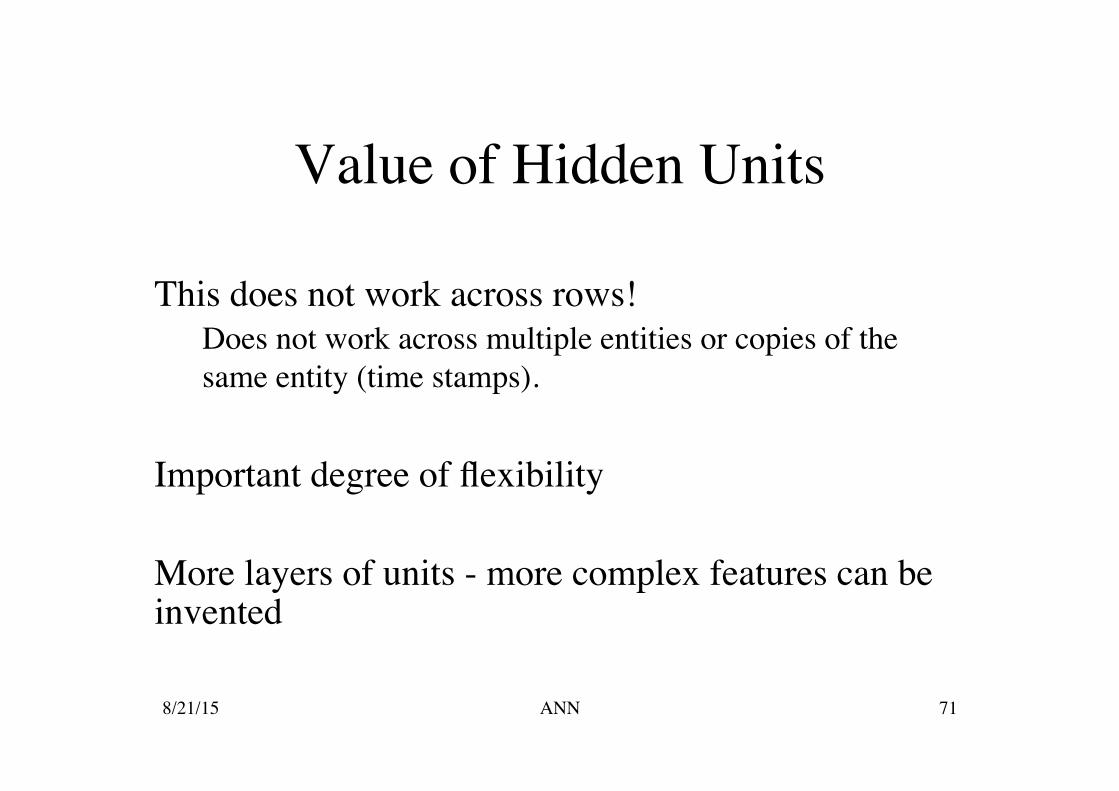
Value of Hidden Units

This does not work across rows! Does not work across multiple entities or copies of the same entity (time stamps).

Important degree of flexibility More layers of units - more complex features can be invented

8/21/15 71 ANN

Hidden Unit Encoding

8/21/15 72 ANN

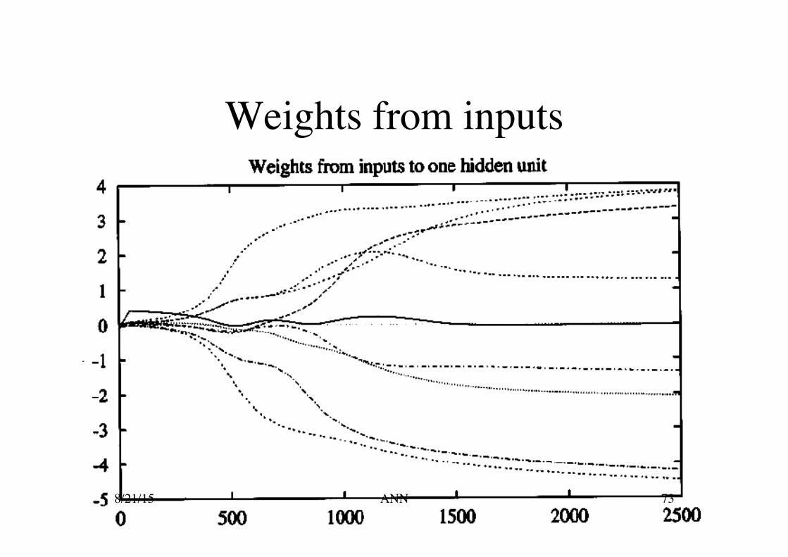
Weights from inputs

8/21/15 73 ANN

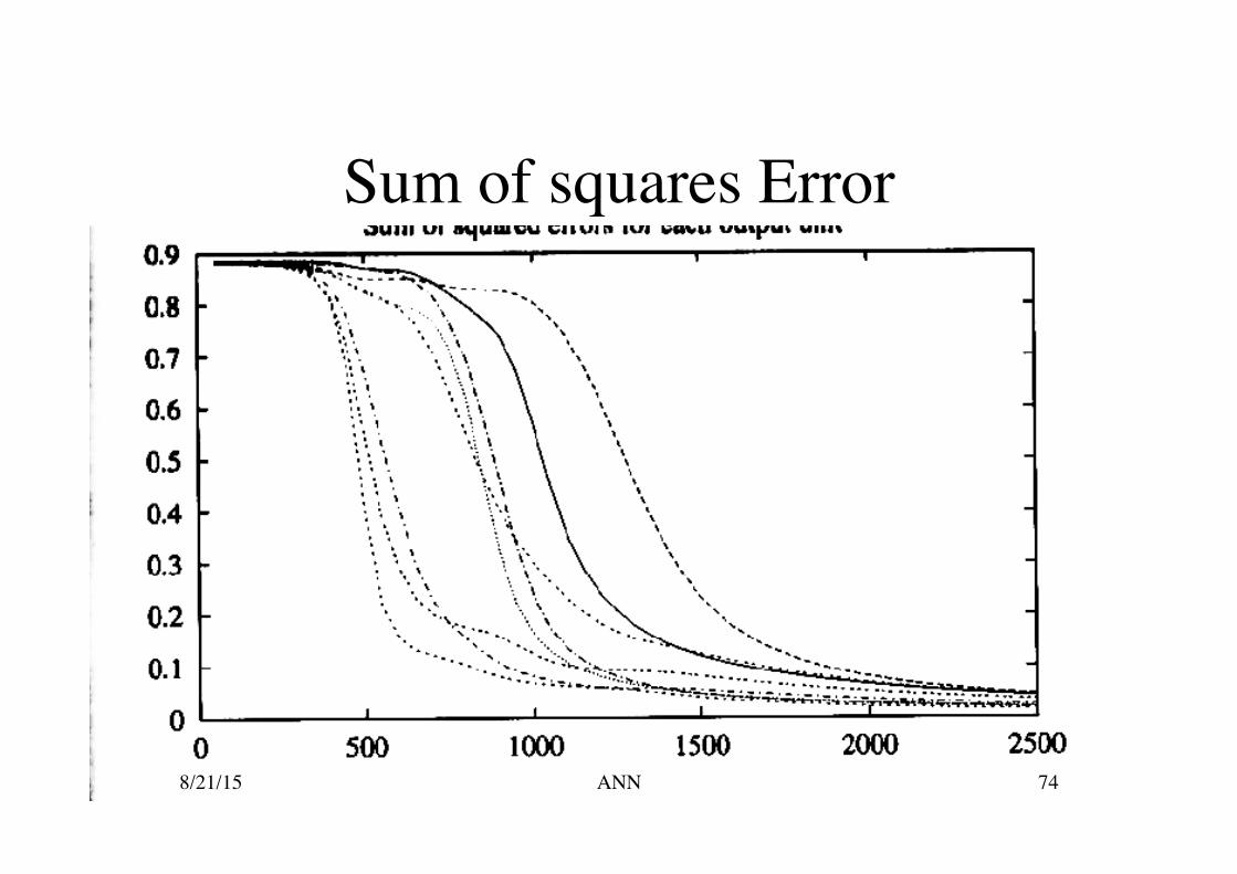
Sum of squares Error

8/21/15 74 ANN

Overfitting and Stopping Criteria 1.  Train until the Error on the training examples

falls below some level Why does overfitting tend to occur in later iterations? Initially weights are set to small random numbers, as training

proceeds weights change to reduce error over the training data & complexity of the decision surface increases, given enough iterations can overfit.

Weight decay - decreases each weight by a small factor on each

iteration - intuition keep weight values small to bias against complex decision surfaces

do complex decision surfaces need to have high weights???

8/21/15 75 ANN

Continued 2.  Stop when you reach the lowest error on the

validation set. Keep current ANN weights and the best-performing weights thus far

measured by error over the validation set Training is terminated once the current weights reach a significantly

higher error over the validation set Care must be taken to avoid stopping too soon!! If data is too small can do k-fold cross validation (remember to use

just to determine the number of iterations!) then train over whole dataset (same in decision trees)

8/21/15 76 ANN

Error Plots

8/21/15 77 ANN

Face Recognition Task 20 people 32 images per person Varying expression, direction looking, wearing sunglasses, background,

clothing worn, position of face in image. 624 greyscale images, resolution 120x128, each pixel intensity ranges

from 0 to 255. Could be many targets: identity, direction, gender, whether wearing

sunglasses - All can be learned to high accuracy. We consider direction looking.

8/21/15 78 ANN

Input Encoding

How encode the image? Use 102x128 inputs? Extract local features: edges, regions of uniform

intensity - how handle a varying number of features per image?

8/21/15 79 ANN

Actual Input Encoding Used Encode image in 30x32 pixel intensity values, one network input per pixel pixel intensities were linearly scaled from 0 to 255 down to 0 to 1.

Why?

8/21/15 80 ANN

Coarse Resolution Summary The 30x32 grid is a coarse resolution summary. Coarse pixel intensity is a mean of the corresponding high pixel intensities Reduces computational demands while maintaining sufficient resolution to correctly classify images

Same as ALVINN except there a represented pixel was chosen randomly for efficiency

8/21/15 81 ANN

Output Encoding A single output unit,

assigning 0.2, 0.4, 0.6, 0.8 as being left, right, up and straight

OR 4 output nodes and choose the highest-valued output as the

prediction (1-of-n output encoding) OR 4 separate neural networks with 1 output each 8/21/15 82 ANN

Output Encoding Issues Is “left” really closer to “right” then it is to “up”? 4 outputs gives more degrees of freedom to the

network for representing the target function (4x #hidden units instead of 1x)

The difference between the highest valued output

and the second highest valued output gives a measure of the confidence in the network prediction

8/21/15 83 ANN

Target Values

What should the target values be? Could use <1,0,0,0> but we use <0.9,0.1,0.1,0.1> sigmoid units can’t produce 0 and 1 exactly with

finite weights so gradient descent will force the weights to grow without bound

8/21/15 84 ANN

Network Graph Structure How many units and how to interconnect? Most common - layer units with feedforward

connections from every unit in one layer to every unit in the next.

The more layers the longer the training time. We choose 1 hidden layer and 1 output layer. 8/21/15 85 ANN

Hidden Units How many hidden units?

3 units = 90% accuracy, 5 minutes learning time 30 units = 92% accuracy, 1 hr learning time

In general there is a minimum number of hidden units needed above that the extra hidden units do not dramatically effect the accuracy, provided cross-validation is used to determine how many gradient descent iterations should be performed, otherwise increasing the number of hidden units often increases the tendency to overfit the training data.

8/21/15 86 ANN

Other Algorithm Parameters Learning rate, η, 0.3 Momentum, α, 0.3 Lower values produced equivalent generalization but

longer training times, if set too high training fails to converge to a network with acceptable error.

Full gradient descent was used (not the stochastic

approximation).

8/21/15 87 ANN

More Parameters

Network weights in the output units were initialized to small random values, but the input unit weights were initialized to zero. It yields a more intelligible visualization of the

learned weights without noticeable impact on generalization accuracy.

8/21/15 88 ANN

Still More Parameters The number of training iterations was selected by partitioning

the available data into a training set and a separate validation set.

GD was used to minimize the error over the training set and

after every 50 gradient descent steps the network performance was evaluated over the validation set.

The final reported accuracy was measured over yet a third set

of test examples that were not use to influence the training.

8/21/15 89 ANN

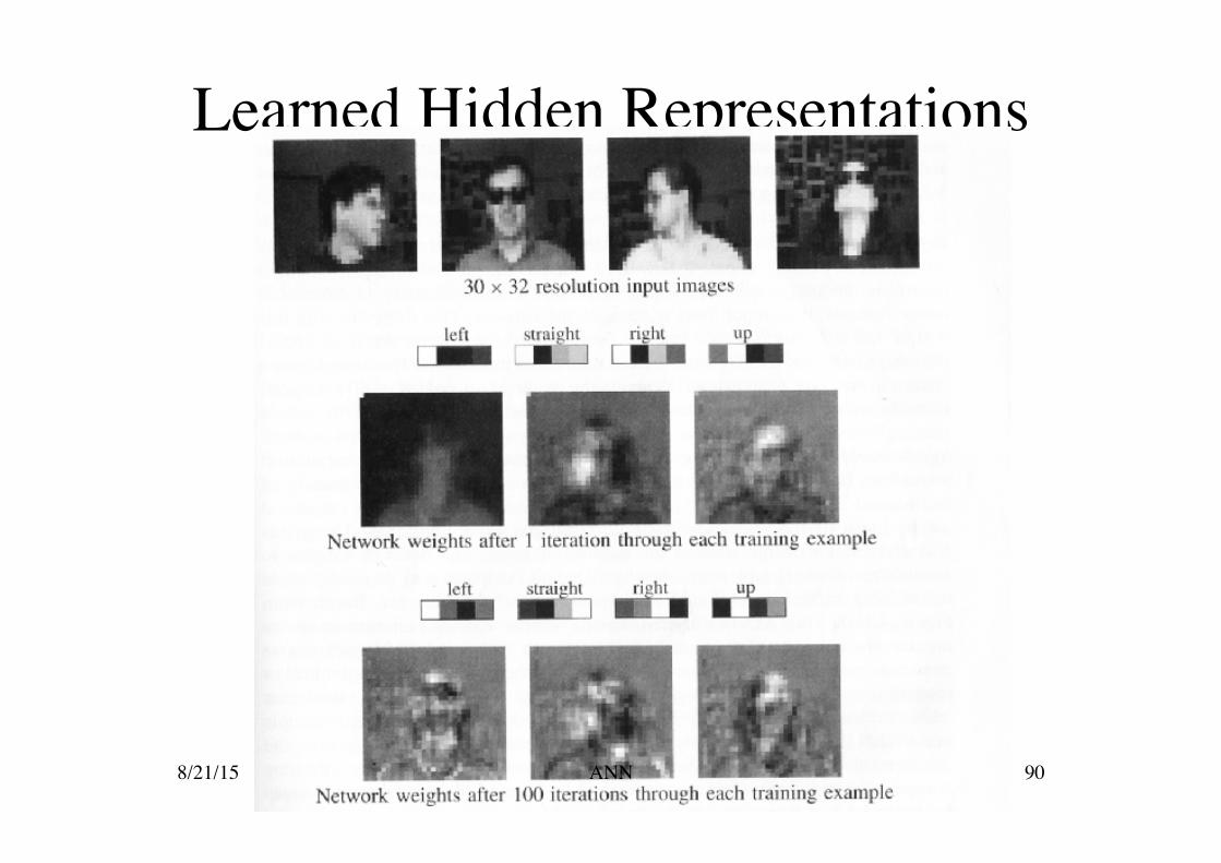
Learned Hidden Representations

8/21/15 90 ANN

Advanced Topics

Alternative Error Functions Alternative Error Minimization Procedures Recurrent Networks Dynamically Modifying Network Structure 8/21/15 91 ANN

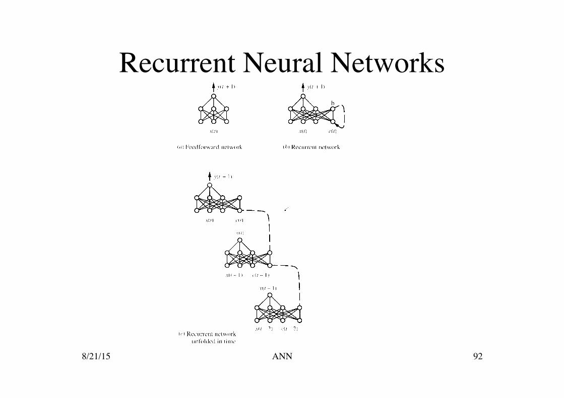
Recurrent Neural Networks

8/21/15 92 ANN

Problems with NN

A lot of parameters Adding random input variables or output

variables makes it work better Humans can’t understand the results 8/21/15 93 ANN

Summary Practical method for learning real-valued and vector-valued

functions over continuous and discrete-valued attributes Robust to noise in the training data Backpropagation algorithm is the most common Hypothesis space: all functions that can be represented by

assigning weights to the fixed network of interconnected units Feedforward networks containing 3 layers can approximate any

function to arbitrary accuracy given sufficient number of units in each layer

8/21/15 94 ANN

Summary II Networks of practical size are capable of representing a rich space

of highly nonlinear functions Backpropagation searches the space of possible hypotheses using

gradient descent (GD) to iteratively reduce the error in the network to fit the training data.

GD converges to a local minimum in the training error with

respect to the network weights Backpropagation has the ability to invent new features that are not

explicit in the input

8/21/15 95 ANN

Summary III Hidden units of multilayer networks learn to represent

intermediate features (e.g., face recognition) Overfitting is an important issue (caused by overuse of

accuracy IMHO) Cross-validation can be used to estimate an appropriate

stopping point for gradient descent Many other algorithms and extensions.

8/21/15 96 ANN