artificial intelligence heuristics for planning with penalties - dtic
TRANSCRIPT

Artificial Intelligence 172 (2008) 1579–1604
Contents lists available at ScienceDirect
Artificial Intelligence
www.elsevier.com/locate/artint
Heuristics for planning with penalties and rewards formulated in logicand computed through circuits
Blai Bonet a,∗, Héctor Geffner b
a Departamento de Computación, Universidad Simón Bolívar, Caracas, Venezuelab Departamento de Tecnología, ICREA & Universitat Pompeu Fabra, 08003 Barcelona, Spain
a r t i c l e i n f o a b s t r a c t
Article history:Received 17 August 2007Received in revised form 2 March 2008Accepted 6 March 2008Available online 29 March 2008
Keywords:PlanningPlanning heuristicsPlanning with rewardsKnowledge compilation
The automatic derivation of heuristic functions for guiding the search for plans is afundamental technique in planning. The type of heuristics that have been considered sofar, however, deal only with simple planning models where costs are associated withactions but not with states. In this work we address this limitation by formulating amore expressive planning model and a corresponding heuristic where preferences in theform of penalties and rewards are associated with fluents as well. The heuristic, that isa generalization of the well-known delete-relaxation heuristic, is admissible, informative,but intractable. Exploiting a correspondence between heuristics and preferred models,and a property of formulas compiled in d-DNNF, we show however that if a suitablerelaxation of the domain, expressed as the strong completion of a logic program withno time indices or horizon is compiled into d-DNNF, the heuristic can be computed forany search state in time that is linear in the size of the compiled representation. Thisrepresentation defines an evaluation network or circuit that maps states into heuristicvalues in linear-time. While this circuit may have exponential size in the worst case, asfor OBDDs, this is not necessarily so. We report empirical results, discuss the applicationof the framework in settings where there are no goals but just preferences, and illustratethe versatility of the account by developing a new heuristic that overcomes limitations ofdelete-based relaxations through the use of valid but implicit plan constraints. In particular,for the Traveling Salesman Problem, the new heuristic captures the exact cost while thedelete-relaxation heuristic, which is also exponential in the worst case, captures only theMinimum Spanning Tree lower bound.
© 2008 Elsevier B.V. All rights reserved.
1. Introduction
The automatic derivation of heuristic functions from problem descriptions in Strips and other action languages has beenone of the key developments in recent planning research [14,51]. Provided with these heuristics, the search for plans be-comes more focused, and if the heuristics are admissible (do not overestimate), the optimality of plans can be ensured[55]. The type of heuristics that have been considered so far, however, have serious limitations. Basically they are eithernon-admissible [12,40] or not sufficiently informative [39], and in either case they are restricted to cost functions whereplan costs depend on actions but not on states. As a result, the tradeoffs that can be expressed are limited; in particular, itis not possible to state a preference for achieving or avoiding an atom p in the way to the goal, or take this preference intoaccount when searching for plans.
* Corresponding author.E-mail addresses: [email protected] (B. Bonet), [email protected] (H. Geffner).
0004-3702/$ – see front matter © 2008 Elsevier B.V. All rights reserved.doi:10.1016/j.artint.2008.03.004

1580 B. Bonet, H. Geffner / Artificial Intelligence 172 (2008) 1579–1604
In this work, we address these limitations by formulating the derivation of heuristic functions in a logical framework.We have shown elsewhere that the heuristic represented by the planning graph [11] can be understood as a precise formof deductive inference over the stratified theory that encodes the problem [31]. Here our goal is not to reconstruct anexisting heuristic but to use a logical formulation for producing a new one. The advantages of a logical framework aretwo: the derivation of heuristic information is an inference problem that can be made transparent with the tools of logic,and powerful algorithms have been developed that make certain types of logical inferences particularly effective. The latterincludes algorithms for checking satisfiability [52], computing answer sets [61], and compiling CNF formulas into tractablerepresentations [25].
Here we consider preferences over actions a and fluents p that are expressed in terms of real costs c(a) and c(p). Actioncosts are assumed to be non-negative, while fluent costs can be positive or negative. Negative costs express rewards. Thecost of a plan is assumed to be given by the sum of the action costs plus the sum of the atom costs for the atoms madetrue by the plan. We are interested in computing a plan with minimum cost. This is a well defined task, which as we willsee, remains well-defined even when there are no goals but just preferences. In such a case, the best plans simply try tocollect rewards while avoiding penalties, and if there are no rewards, since action costs are non-negative, the best plan isempty.
The cost model is not fully general but is considerably more expressive than the one underlying classical planning. Aswe will see, the model generalizes recent formulations that deal with over-subscription or soft goals [60,64], which in oursetting can be modeled as terminal rewards, rewards that are collected when the propositions hold at the end of the plan.On the other hand, the costs and rewards are combined additively, so unlike other recent frameworks [8], partially-orderedpreferences are not handled.
The definition of the planning model is motivated by the desire to have additional expressive power and a principledand feasible computational approach for dealing with it. For this, we want a useful heuristic, with a clear semantics, capableof capturing interesting cost tradeoffs, and a feasible algorithm for computing it. We will be able to express in the model,for example, navigation problems where coins of different values are to be collected by avoiding as much as possible certaincells, or blocks-world problems where a tallest tower is to be constructed, or where the number of blocks that touch thetable is to be minimized. In order to test the effectiveness of the approach we will also consider classical planning taskswhere we will assess the approach empirically in relation to existing heuristics and planners.
The heuristic h+c that we develop is simple and corresponds to the optimal cost of the relaxed problem where the
delete-lists of all actions are ignored [12]. Since searching with this heuristic, even in the classical setting, involves anintractable computation in every state s visited [15], planners such as HSP and FF resort to polynomial but non-admissibleapproximations [12,40]. In this work, while considering the more general cost structure, we take a different approach: wecompute the heuristic h+
c for each search state, but pay the price of an intractable computation only once, as preprocessing.This preprocessing yields what can be deemed as an evaluation network or circuit where we can plug any search stateand obtain its heuristic value in linear time. Of course, the time to construct this evaluation network and the size of thenetwork may both be exponential, yet this is not necessarily so. The evaluation network, indeed, is nothing else but thedirected acyclic graph that results from compiling a relaxation of the planning theory into d-DNNF, a form akin to OBDDsintroduced in [21,22] that renders efficient a number of otherwise intractable queries and transformations [25]. The heuristicvalues are then obtained as the cost of the ‘best’ models, which can be computed in linear time once the relaxed theory iscompiled into d-DNNF [26].
The framework defined by the formulation of the heuristic h+c in terms of logic and their computation in terms of
compiled d-DNNF representations is then evaluated empirically over a broad set of problems, where the heuristic is used toguide the search for optimal plans.
An important characteristic of the logical encoding of the delete-relaxation heuristic is that unlike the standard logicalencodings of planning problem [44], no explicit temporal stratification in the form of time indices or horizons is needed. Thisfollows from the use of positive logic programs for expressing the effects of the actions as an intermediate representation,and the focus on the models that are minimal in the sense that true fluents must have a well-founded justification. Suchminimal models capture an implicit stratification that is in correspondence with the explicit temporal stratification adoptedby the standard logical approaches to planning. A concrete result of this implicit stratification is that the resulting heuristicestimates the true optimal cost of the problem, and not the optimal cost given a specific temporal horizon.
The paper is a revised version of [13] where the results are extended to a new class of heuristics that complement theuse of the delete-relaxation with valid plan constraints.1 Valid plan constraints are formulas defined over the set of actionand fluent symbols that are satisfied by some optimal plan. Making valid plan constraints explicit in a problem hence doesnot affect the true cost of a problem but can boost the value of the heuristic while keeping it admissible. We show forexample the new heuristic is optimal for problems like the Traveling Salesman Problem (TSP), where the delete-relaxationheuristic h+
c , which is also exponential in the worst case (unless P = NP), yields only the Minimum Spanning Tree (MST)lower bound (for references on the TSP and MST; see [18,48,56]).
The plan for the paper is the following: we present in order the cost model, the heuristic h+c , the correspondence
between h+c and the rank of a suitable propositional theory, and the computation of the heuristic for any state in terms
1 We also correct a mistake in [13] where a planning language with conditional effects is used although some of the results apply only to Strips.

B. Bonet, H. Geffner / Artificial Intelligence 172 (2008) 1579–1604 1581
of a suitable d-DNNF compilation of the theory. We then deal with the search algorithm, that must handle negative costs,present the experimental results, and consider the more powerful heuristic that arises when plan constraints are taken intoaccount. We then summarize the main contributions, and discuss related work and open problems.
2. Planning and cost model
We consider Strips planning problems P = 〈F , I, O , G〉 where F is the set of relevant atoms or fluents, I ⊆ F and G ⊆ Fare the initial and goal situations, and O is a set of (grounded) actions a with precondition, add, and delete lists Pre(a),Add(a), and Del(a).
A plan π for a problem P = 〈F , I, O , G〉 is an applicable action sequence a0,a1, . . . ,an with ai ∈ O for i = 0, . . . ,n, thattransforms the initial state s0 associated with I into a final state sn+1 where the goal G holds. States are sets of fluents,the initial state s0 is I , and the state si+1 that follows action ai in state si is si+1 = si + Add(ai) − Del(ai), where ‘+’ and‘−’ stand for set union and difference respectively. The action ai is applicable in si if Pre(ai) ⊆ si , and the action sequencea0,a1, . . . ,an is applicable if each action is applicable in the state that results from the previous actions in the sequence.
We are interested in plans π for P that minimize a cost measure c(π). The cost c(π) of a plan π in classical planningis associated with the number of actions in the plan; a cost measure that is usually written as |π | and can also be expressedas:
c(π) =∑ai∈π
c (1)
where c is a positive constant equal to 1. This cost structure however is often too limited. An immediate generalization canbe obtained by assuming that actions a have a non-uniform and non-negative cost c(a) so that the cost of a plan becomes:
c(π) =∑ai∈π
c(ai). (2)
The classical cost structure follows then by setting the action costs c(a) to 1. Interestingly, some of the heuristics developedfor classical planning, including the additive [12] and hm heuristics [39], deal easily with non-uniform action costs, whileothers, such as the heuristics underlying Graphplan [11] and the FF planner [40], which are defined in terms of planninggraphs, do not.
A further generalization can be obtained by making costs dependent not only on the actions made in the plan, but alsoon the states that are traversed:
c(π) =∑ai∈π
c(ai, si). (3)
Here c(ai, si) stands for the cost of executing action ai in the state si that results from the execution of the previous actionsin the plan.
In the general cost model captured by (3), costs may depend on both actions and states, in (2), they may depend on theactions only, while in (1) they may depend on neither one. In this work, we deal with plan costs that depend on both theactions and the states but in the restricted form:
c(π) =∑ai∈π
c(ai) +∑
p∈F (π)
c(p) (4)
where F (π) is the set of fluents made true by plan π at any time point during the plan execution, and c(p) is the cost of fluentp ∈ F .
In comparison with (3), the cost model given by (4) defines the costs c(ai, si) additively in terms of the action costs c(ai)
and fluent costs c(p). The costs c(a) of actions is assumed to be non-negative, while the costs c(p) of fluents can be positive,negative, or zero (by default). Positive fluents costs are called penalties, while negative fluents costs are called rewards.
For optimal plans to have always a bounded cost, the plan cost measure c(π) defined by (4) counts fluent costs c(p) atmost once.2 Without this restriction, a plan could get an infinite reward by achieving an atom p with negative cost c(p)
and then ‘waiting’ doing something irrelevant.Given the cost of plans c(π) captured by (4), we are interested in the plans π that minimize c(π); these are the optimal
or best plans. If there is a plan at all, this optimization problem is well defined, although the best plan is not necessarilyunique. We denote by c∗(P ) the cost of a best plan for problem P with respect to the cost function c over actions andfluents
c∗(P )def= min
{c(π): π is a plan for P
}(5)
2 This restriction makes the model non-markovian in the sense that the contribution of action ai in the state si is c(ai) plus the cost c(p) of the atoms pin the next state si+1 that have not been true in earlier states. We will say more about this when discussing the search for optimal solutions in this modeland the information that must be kept in the search nodes.

1582 B. Bonet, H. Geffner / Artificial Intelligence 172 (2008) 1579–1604
and set c∗(P ) to ∞ when P admits no plan. Clearly, when c(a) = 1 and c(p) = 0 for all actions a and fluents p, the costcriterion of classical planning is obtained where c∗(P ) measures the minimum number of actions needed to solve P . Theresulting framework, however, is more general, as costs on both actions and fluents can be expressed, and the latter can beeither positive or negative. Indeed, it is possible to model problems with no goals but just preferences expressed in the formof rewards. In such a case, the empty plan is optimal if there are no rewards (action costs are assumed to be non-negative),but other plans may have a smaller, and thus negative cost, when rewards are present. In general, the best plans mustachieve the goal by trading off action and fluent costs.
We will call the planning cost model captured by (4) the penalties and reward model, abbreviated as pr. This cost modelis similar to the one used in over-subscription planning where due to constraints or preferences, it may not be possible orconvenient to achieve all the goals [60,64]. There are two important differences though. The first is that in pr atoms can berewarded when they are achieved anytime during the execution of the plan, not only when they are achieved at the end ofthe plan. The second is that such atoms may express either penalties or rewards. If they express penalties (positive costs),they are not atoms to be achieved but to be avoided during the execution.
In order to capture preferences on end states as opposed to preferences on intermediate states, when required, we con-sider the use of an special End action with zero cost that must terminate all plans, whose preconditions are the goals G ofthe problem, and whose effect is a dummy goal done. In order for such an action to terminate all plans it is sufficient tohave an additional fluent not_done, initially true, that is a precondition of all actions, and that is deleted by the action End.With this convention, the representation of preferences on end states becomes possible by simply adding conditional effectsto the action End. While we assume that the language is Strips and hence that conditional effects are not accommodated,the generalization to such an extension (a final action with conditional effects) is straightforward and is supported in theplanner.
3. Modeling
The cost model for planning formulated above is simple but flexible. Some preference patterns that can easily be ex-pressed are:
• Terminal Costs: an atom p can be rewarded or penalized if true at the end of the plan by introducing a new atom p′ ,initialized to false along with the conditional effect p → p′ for the action End. A reward or penalty c(p′) on p′ thencaptures a reward or penalty on p at the end of the plan. In such a case, we call c(p′) a terminal cost on p and p′ aterminal atom.
• Goals: once costs on terminal states can be expressed, goals are not strictly required. Semantically, a hard goal canbe modeled as a sufficiently high terminal reward. Computationally, however, the first option will usually yield betterresults.
• Soft Goals: soft goals can be modeled as terminal rewards, and the best plans will achieve them depending on the costsinvolved.
• Preferences on Literals: while the model assumes that costs are associated with positive literals p but no negative ones,standard planning transformation techniques can be used to add a new atom p′ that is true exactly when p is false[33,53]. Preferences on the negation of p can then be expressed as preferences on p′ .
• Rewards on Conjunctions: it is possible to reward states in which a set of atoms p1, . . . , pn is true by means of anaction Collect(p1, . . . , pn) with preconditions p1, . . . , pn , and effect p, where p is a new atom that is rewarded. Thesame trick however does not work for expressing penalties on conjunctions. The reason is that optimal plans will chooseto collect a free reward if possible, but will never choose to collect a free cost (as would be required if the atom p werea penalty and not a reward).
As an illustration, a blocks-world problem where the number of blocks that touch the table is to be kept to a minimum(at the price of obtaining possibly a longer plan) can be obtained by penalizing the atoms on(x, table) for blocks x. Moreinterestingly, the problem of building the tallest possible tower results from assigning terminal rewards to the atoms on(x, y)
for all the blocks x and y (with non-terminal rewards instead, the best plans would move the blocks around placing everyblock on top of every other block to collect all rewards associated with the atoms on(x, y)). If actions have positive costs,the best plans will be the ones that achieve a tallest tower in a minimum number of steps (i.e., choosing one of theexisting tallest towers as the basis). Likewise, problems where an agent is supposed to pick up some coins while avoidinga dangerous ‘wumpus’, can be modeled by rewarding the atoms have(coini) and penalizing the atoms at(x, y) where x, y isthe position of the wumpus.3
Among preference patterns that the pr cost model does not capture in a natural way are positive costs on sets of atoms(mentioned above) and partial preferences where certain costs are not comparable [6,8].
The pr model can be extended to deal with repeated penalties or rewards, as when a cost is paid each time an atomis made true. We do not consider such an extension in this work, however, for two reasons: semantically, with repeated
3 The Wumpus problem in [59] is more interesting though as it involves uncertainty and partial observability, issues that are not addressed in the pr
model.

B. Bonet, H. Geffner / Artificial Intelligence 172 (2008) 1579–1604 1583
rewards, some problems do not have a well-defined cost (cyclic plans may accumulate an infinite reward);4 and computa-tionally, the proposed heuristics do not capture the specific features of such a model, even if as we will see, they wouldremain admissible then.
4. Heuristic h+c
Heuristics are fundamental for searching in large spaces. In the classical setting, several effective heuristics have beenproposed, most of which are defined in terms of the delete-relaxation: a simplification of the problem where the delete-lists of the operators are dropped. Delete-free planning is simpler than planning in the sense that plans can be generatedin polynomial time; still optimal delete-free planning is intractable too [15]. Thus, on top of this relaxation, the heuristicsused in many classical planners rely on other simplifications; the formulation in [40] drops the optimality requirement inthe relaxed problem, while the one in [14,51], assumes that subgoals are independent. In both cases, the resulting heuristicsare not admissible.
The heuristic that we formulate for the pr model builds on and extends the optimal delete-relaxation heuristic proposedin classical planning. If P+ is the delete-relaxation of problem P , i.e., the planning problem obtained by dropping all thedelete-lists from the actions in P , the heuristic h+
c (P ) that provides an estimate of the cost of solving P given the costfunction c is defined as
h+c (P )
def= c∗(P+), (6)
where c∗(P+) is the optimal cost of the delete-relaxation. For the 0/1 cost function that characterizes classical planning,where the cost of all atoms is 0 and the cost of all actions is 1, this definition yields the (optimal) delete-relaxation heuristicwhich provides an estimate on the number of steps to the goal. This heuristic is admissible and tends to be quite informativetoo (see the empirical analysis in [41]). Expression (6) generalizes this heuristic to the larger class of cost functions whereactions may have non-uniform costs and atoms can be rewarded or penalized, and where it remains admissible too:5
Proposition 1 (Admissibility). The heuristic h+c (P ) is admissible; i.e. h+
c (P ) � c∗(P ).
If we let P [I = s] and P [G = g] refer to the planning problems that are like P but with initial and goal situationsI = s and G = g respectively, then (optimal) forward heuristic-search planners aimed at solving P need to compute theheuristic values h+
c (P [I = s]) for all states s encountered, while regression planners need to compute the heuristic valuesh+
c (P [G = g]) for all encountered subgoals g . Since each such computation is intractable, even for the 0/1 cost function,classical planners like HSP and FF settle on polynomial but non-admissible approximations. In this work we take a differentpath: we use the h+
c heuristic in the more general cost setting, but rather than performing an intractable computation forevery search state encountered, we perform an intractable computation only once. For this, we establish a correspondencebetween heuristic values and ranks of a propositional theory, which can be computed in polynomial time provided that thetheory is compiled in a suitable form.
5. Heuristics, preferred models, and d-DNNF
Following [43,44], a propositional encoding of a sequential planning problem P = 〈F , I, O , G〉 with horizon n can beobtained by introducing fluent and action variables pi and ai for each fluent p, action a, and time step i in a theory Tn(P )
comprised of the following formulas:
1. Init: p0 for p ∈ I , ¬q0 for q ∈ F − I2. Goal: pn for p ∈ G3. Actions: For i = 0,1, . . . ,n − 1 and all a ∈ O
ai ⊃ pi for p ∈ Pre(a)
ai ⊃ qi+1 for each positive effect q ∈ Add(a)
ai ⊃ ¬qi+1 for each negative effect q ∈ Del(a)
4. Frame: For i = 0, . . . ,n − 1 and all p ∈ Fpi ∧ (∧
a:p∈Del(a) ¬ai) ⊃ pi+1
¬pi ∧ (∧a:p∈Add(a) ¬ai
) ⊃ ¬pi+1
5. Seriality: For i = 0,1, . . . ,n − 1 and a �= a′ , ¬(ai ∧ a′i).
For a sufficiently large horizon n, the models of the propositional theory Tn(P ) are in correspondence with the plans for P :each model encodes a plan, and each plan determines a model.
4 This same problem arises in Markov Decision Processes where the usual work around is to discount future costs [10].5 Formal proofs of the results in the paper can be found in Appendix A.

1584 B. Bonet, H. Geffner / Artificial Intelligence 172 (2008) 1579–1604
For any cost function c, if we define the rank r(M) of a model M as the cost c(π) of the plan that the model M makestrue, and define the rank r∗(T ) of a theory T as the rank of its best model
r∗(T )def= min
M| Tr(M) (7)
with r∗(T ) = ∞ if T has no models, it follows then that the cost of P and the rank of its propositional encoding Tn(P ) arerelated as follows:
Proposition 2 (Costs and Ranks). For a sufficiently large time horizon n (exponential in the worst case), c∗(P ) = r∗(Tn(P )), where therank r(M) of a model M of Tn(P ) is given by the cost of the plan defined by M.
This correspondence between the cost of a planning problem and the rank of a propositional theory, follows directlyfrom the definitions and does not give us much unless we have a way to derive theory ranks effectively. A result in thisdirection comes from [26] that shows how to compute theory ranks r∗(T ) efficiently when r is a literal-ranking functionand the theory T is in d-DNNF [22]. A literal ranking function ranks models in terms of the rank of the literals l that theyrender true:6
r(M)def=
∑l:M| l
r(l). (8)
For literal-ranking functions r and propositional theories T compiled into d-DNNF, Darwiche and Marquis show that
Theorem 3 (Darwiche and Marquis). If a propositional theory T is in d-DNNF and r is a literal-ranking function, then the rank r∗(T )
can be computed in time linear in the size of T .
This result suggests that we could compute the optimal cost c∗(P ) of P by compiling first the theory Tn(P ) into d-DNNF and then computing its rank r∗(Tn(P )) in time linear in the size of the compilation. There are two obstacles to thishowever. The first is that the model ranking function r(M) = c(π(M)) in Theorem 2 is defined in terms of the cost of theatoms made true during the execution of the plan, not in terms of the literals true in the model, and hence it is not exactlya literal-ranking function such as (8). The second, and more critical, is that the horizon n needed for ensuring Theorem 2 isnormally too large for Tn(P ) to compile. We show below though that these two problems can be handled better when thecomputation of the heuristic h+
c (P ), that approximates the real cost c∗(P ), is considered instead.Before focusing on the logical encodings required for computing the heuristics h+
c (P [I = s, G = g]) for any state s andsubgoal g in linear-time from a suitable d-DNNF compilation, let us briefly recall how d-DNNF formulas T are representedand how their ranks r∗(T ), defined by (7) and (8), are computed. A formula T in d-DNNF is a rooted DAG (Directed AcyclicGraph) whose leaves are the positive and negative literals associated with the variables in T along with the constants trueand false, and whose internal nodes stand for conjunctions or disjunctions (AND and OR nodes, respectively). The formulawff (n) associated with the root node n of a d-DNNF formula can be read off recursively from the leaves as follows:
wff (n) =⎧⎨⎩
L if n is a leaf associated with literal L∧i wff (ni) if n is an AND node with children ni∨i wff (ni) if n is an OR node with children ni .
(9)
A d-DNNF formula is thus in Negated Normal Form (NNF) as it contains only the connectives for conjunctions, disjunctions,and negations, and negation occurs only in literals [4]. The d-DNNF formula is a NNF formula represented as a DAG thatsatisfies two conditions. The first is decomposability, that accounts for the ‘D’ in d-DNNF and requires that the subformulasassociated with the children of an AND node, share no variables. The second is determinism, that accounts for the ‘d’ ind-DNNF and requires that the subformulas associated with the children of an OR node, be mutually exclusive.
These two conditions enable a large number of otherwise intractable queries and transformations to be done in timewhich is linear in the size of the DAG representation [25]. For example, the procedure for computing the rank r∗(T ) ofa formula T in d-DNNF can be expressed in terms of the value of the function r∗(n) computed recursively, bottom up asfollows [26]:
r∗(n) =
⎧⎪⎪⎪⎪⎨⎪⎪⎪⎪⎩
0 if n = true
∞ if n = false
r(L) if n = L where L is a literal different than true and false∑i r∗(ni) if n is an AND node with children ni
mini r∗(ni) if n is an OR node with children ni .
(10)
6 Darwiche and Marquis use the name ‘normal weighted bases’ rather than literal-ranking functions.
B. Bonet, H. Geffner / Artificial Intelligence 172 (2008) 1579–1604 1585
The DAG representing the theory T in d-DNNF thus becomes an arithmetic circuit with the leaves replaced by the numbers0, ∞, or r(L) according to whether the leaf is the constant true, false, or the non-constant literal L, and the internal nodesreplaced by sums and minimizations, according to whether they stand for AND or OR nodes. The output of this circuit,computed in time that is linear in the size of the circuit, is the theory rank r∗(T ). For computing in turn the rank r∗(T ∪ S)
of the theory that extends T with a set S of literals over the same language, the same bottom-up procedure working on thecompiled representation of T can be used, treating the leaves n = L as true if L ∈ S , and as false if ¬L ∈ S [26].
Any formula can be compiled into d-DNNF [23]. The time to build the compiled representation and the size of thecompiled representation may both be exponential in the worst case, yet like compilation into OBDDs, a compiled logicalrepresentation commonly used in automated verification [16] and closely related to d-DNNF’s [25], this is not necessarilyso in general. Indeed, the compilation of the theory is exponential (in both time and space in the worst case) in a struc-tural parameter associated with the theory known as the treewidth, which measures the degree of interaction among itsvariables; see [21,24].
Once a correspondence between the heuristic h+c (P ) and the rank r∗(T ) of a suitable propositional encoding is estab-
lished, we will see that an arithmetic circuit like that one described above can be used to map any state s and subgoal ginto the heuristic value h+
c (P [I = s, G = g]).
5.1. Stratified encodings
Since the heuristic h+c (P ) is defined in terms of the optimal cost of the relaxed, delete-free problem P+ , it is natural
to consider the computation of the heuristic in terms of the theory Tn(P+) of the relaxed problem. We will do this belowbut first we will simplify the theory Tn(P+) by dropping the seriality constraints that are no longer needed in the delete-freesetting where any parallel Strips plan can be serialized retaining its cost. In addition, we will drop from Tn(P+) the init andgoal clauses as we want to be able to compute the heuristic values h+
c (P [I = s]) and h+c (P [G = g]) for any possible initial
state s and subgoals g that might arise in a progression or regression search respectively. We call the set of clauses thatare left in Tn(P+), the stratified (relaxed) encoding and denote it by T +
n (P ). Later on we will consider another encoding thatdoes not involve a temporal stratification at all.
The first crucial difference between the problem P and its delete-free relaxation P+ is the horizon needed for havinga correspondence between models and plans. For P , the optimal plans may have exponential length due to the number ofdifferent states that a plan may visit. On the other hand, the optimal plans for P+ have at most linear length, as withoutdeletes, actions can only add atoms, and thus the number of different states that can be visited is bounded linearly by thenumber of fluents.
The second difference is that the optimal cost of the delete-free problem can be put in correspondence with the rankof its propositional encoding using a simple literal-ranking function compatible with Theorem 3, as any atom achieved in adelete-free plan remains true until the end of the plan.
If we let I0 and Gn stand for the init and goal clauses in the theory Tn(P ) that capture the initial and goal situationsI = s and G = g respectively, the following correspondence between heuristic values and theory ranks can be established:
Proposition 4 (Heuristics and Ranks). For a sufficiently large horizon n (linear in the worst case) and any initial and goal situations sand g,
h+c
(P [I = s, G = g]) = r∗(T +
n (P ) ∪ I0 ∪ Gn),
where r is the literal ranking function such that r(pn) = c(p) for every fluent p, r(ai) = c(a) for every action a and i ∈ [0,n − 1],otherwise r(l) = 0.
Exploiting then Theorem 3 and the ability of d-DNNF formulas to be conjoined with literals in linear-time, we get:
Theorem 5 (Compilation and Heuristics). Let Πn(P ) refer to the compilation of theory T +n (P ) into d-DNNF where n is a sufficiently
large horizon (linear in the worst case). Then the heuristic values h+c (P [I = s, G = g]) for any initial and goal situations s and g,
and any cost function c, can be computed from Πn(P ) in linear time.
This theorem tells us that a single compilation suffices for computing a huge set of heuristic values in time that is linearin the size of the compilation. The heuristic values h+
c (P [I = s, G = g]) provide estimates of the cost of achieving any goalg from any initial state s. During a forward search, however, only the values h+
c (P [I = s]) are needed, while in a regressionsearch, only the values h+
c (P [G = g]) are needed. The formulation, however, yields a larger number of heuristic values thatcan be used, for example, in a bidirectional search.
5.2. Logic programming encodings
The encoding Tn(P ) for computing the optimal cost c∗(P ) of P requires an horizon n that is exponential in the worstcase, while the encoding T +
n (P ) for computing the heuristic h+c (P ) requires an horizon that is only linear. Still, a more

1586 B. Bonet, H. Geffner / Artificial Intelligence 172 (2008) 1579–1604
compact encoding for computing h+c , which requires no time or horizon at all, can be obtained. We call it the LP encoding as
it is obtained from a set of positive Horn clauses [47].The LP encoding of a planning problem P for computing the heuristic h+
c is obtained from the propositional LP rules ofthe form
p ← Pre(a),a (11)
for each positive effect p ∈ Add(a) associated with an action a with preconditions Pre(a) in P . For convenience, as we explainbelow, for each atom p in P , we introduce also a ‘dummy’ action set(p) with unique effect p and no precondition encodedas:
p ← set(p). (12)
These actions will be formal devices for ‘setting’ the initial situation to s when computing the heuristic values h+c (P [I = s])
in a progression search. No such encoding trick is needed for the goals g in a regression search.The LP encoding, that will enable us to compute the h+
c heuristic in a more effective way, has two features that distin-guish it from the previous stratified encodings. The first is that there are no time indices. These indices are not necessaryas we will focus on a class of minimal models of the program that have an implicit stratification which is in correspondencewith the temporal stratification. Such minimal models will be grounded on the actions as all fluents will be required to havea well-founded support based on them. The second distinctive feature is that actions do not imply their preconditions. Thiswill not be a problem either as actions all have non-negative costs and, in this encoding, all require their preconditions inorder to have some effect. So while models that make actions true without their preconditions are possible, such modelswill not be preferred over the same models where such actions are false, and hence they will not affect the rank of thetheory.
For a planning problem P , let L(P ) refer to the collection of rules (11) and (12) encoding the effects of the actions in P ,including the set(p) actions, and let wffc(L(P )) stand for the well-founded fluent completion of L(P ): a completion formuladefined below that forces each fluent p to have a well-founded support. Then if we let I(s) refer to the collection of unitclauses over the variables set(p) that represent a situation s, namely set(p) ∈ I(s) iff p ∈ s, and ¬set(p) ∈ I(s) iff p /∈ s, weobtain that the correspondence between heuristic values and LP encodings becomes:
Proposition 6 (Heuristics and Ranks). For any initial situation s, goal g, and cost functions c,
h+c
(P [I = s, G = g]) = r∗(wffc
(L(P )
) ∪ I(s) ∪ g)
where r is the literal ranking function such that r(l) = c(l) for positive literals l and r(l) = 0 otherwise.
From this result and the properties of d-DNNF formula, we obtain:
Theorem 7 (Main). Let Π(P ) refer to the compilation of theory wffc(L(P )) into d-DNNF. Then for any initial and goal situations sand g, and any cost function c, the heuristic value h+
c (P [I = s, G = g]) can be computed from Π(P ) in linear time.
The well-founded fluent completion wffc(L(P )) picks up the models of the logic program L(P ) that are minimal in the setof fluents given the actions in the model; namely the minimal models of the logic program L(P ) ∪ A for any set of actions Awith the actions in A treated as facts. In such models, fluents have a non-circular support that is based on the actions thatare true in the model. In particular, if L(P ) is an acyclic program, wffc(L(P )) is nothing else but Clark’s completion appliedto the fluents [1,17]. The program L(P ) is acyclic if the directed graph formed by connecting every atom that appears in thebody of a rule to the atom that appears in the head, is acyclic; and Clark’s completion applied to the fluent literals adds theformulas
p ⊃ B1 ∨ · · · ∨ Bn
to each fluent p with rules
p ← Bi
for i = 1, . . . ,n in L(P ), and the formula ¬p when there are no rules for p at all.In the presence of cycles in L(P ), the well-founded fluent completion wffc(L(P )) does not reduce to Clark’s completion,
which does not exclude circular supports. In order to rule out circular supports and ensure that the fluents in the model canbe stratified as in temporal encodings, a stronger completion is needed. Fortunately, this problem has been addressed in theliterature on Answer Set Programming [2,5,34] where techniques have been developed for translating cyclic and acyclic logicprograms into propositional theories whose models are in correspondence with their Answer Sets [9,49]. The logic programL(P ) is a positive logic program whose unique minimal model, for any set of actions, coincides with its unique AnswerSet. The strong completion wffc(L(P )) can thus be obtained from any such translation scheme, with the provision thatonly fluent atoms are completed (not actions). In our current implementation, we follow the scheme presented in [50] thatintroduces new atoms and new rules that provide a consistent, partial ordering on the fluents in L(P ) so that the resultingmodels become those in which the fluents have well-founded, non-circular justifications. This is a polynomial transformationwhich is illustrated in the example below. From now on, wffc(L(P )) will refer to the result of such a translation.

B. Bonet, H. Geffner / Artificial Intelligence 172 (2008) 1579–1604 1587
6. Example
As an illustration of the logical formulation of the delete-relaxation heuristic h+c , consider a simple problem P that
involves three locations A ↔ B ↔ C , such that an agent can move between A and B , between B and C , but cannot movedirectly between A and C .
This problem can be modeled with actions of the form move(x, y) with precondition at(x) and effects at(y) and ¬at(x),for x and y ranging over A, B , and C so that the resulting actions correspond to the allowed transitions. For each suchaction in P , L(P ) contains rules
at(y) ← at(x),move(x, y)
along with
at(y) ← set(at(y)
).
Consider now an initial state s = {at(A)}, a goal g = {at(C)}, and a cost function c(a) = 1 for all actions except for move(A, B)
with cost c(move(A, B)) = 10.The best plan for this state-goal pair in the delete-relaxation is π = {move(A, B),move(B, C)}, which is also the best plan
without the relaxation, so
h+c
(P [I = s, G = g]) = c∗(P [I = s, G = g]) = 11.
Proposition 6 says that this heuristic value must correspond to the rank of the well-founded fluent completion of L(P ),wffc(L(P )), extended with the set of literals given by
I(s) = {set
(at(A)
),¬set
(at(B)
),¬set
(at(C)
)},
and
g = {at(C)
}.
In order to get an intuition for this completion, let us illustrate first why it must be stronger than Clark’s completion. Forthis problem, Clark’s completion for the fluent atoms gives us the theory:
at(C) ≡ (at(B) ∧ move(B, C)
) ∨ set(at(C)
)at(B) ≡ (
at(A) ∧ move(A, B)) ∨ set
(at(B)
) ∨ (at(C) ∧ move(C, B)
)at(A) ≡ (
at(B) ∧ move(B, A)) ∨ set
(at(A)
).
For the literal ranking function r that corresponds to c,7 the best ranked model of Clark’s completion extended with theliterals in I(s) and g , has rank 2 which is different than h+
c (P [I = s, G = g]) = 11. In such a model, the costly move(A, B) ac-tion is avoided, and the fluent at(C) has a circular justification that involves the cheaper actions move(B, C) and move(C, B).This arises because the program L(P ) contains a cycle involving the atoms at(B) and at(C).
In the well-founded completion defined in [50], Clark’s completion is applied to a program which is different than L(P )
and where circularities are broken. For this example, each rule instance
at(y) ← at(x),move(x, y)
in L(P ) is replaced by a collection of rules
rk ← NOTat(y) ≺ at(x),at(x),move(x, y)
at(y) ← rk
at(x) ≺ at(y) ← rk
at(z) ≺ at(y) ← rk,at(z) ≺ at(x)
where z ranges over the locations A, B , and C , and ‘NOT ’ stands for negation as failure. The new rules introduce two newpredicates: one is rk that stands for a unique identifier of the original rule instance in L(P ); the other is ‘≺’ that representsa precedence constraint among the atoms at(A), at(B), and at(C) that form a loop in L(P ) and ensures that the supports inthe resulting models are all well-founded. Thus, the first pair of rules allows the atoms at(x) and move(x, y) to support theatom at(y) when at(x) does not precede at(y), while the third rule ensures that this support makes at(x) precede at(y),and the last rule that the precedence relation is closed under transitivity.
The well-founded fluent completion wffc(L(P )) is the result of applying Clark’s completion to the fluents of the resultingtransformed program. The best model of such a theory extended with the set of literals in I(s) and g as above, contains
7 From Proposition 6, r(l) = c(l) if l is a positive literal and r(l) = 0 otherwise.

1588 B. Bonet, H. Geffner / Artificial Intelligence 172 (2008) 1579–1604
the actions move(A, B) and move(B, C) for a rank of 11, in agreement with the heuristic value h+c (P [I = s, G = g]). The
interpretation that contains the actions move(B, C) and move(C, B) instead, is not a model of the theory, as it requires ajustification of at(B) in terms of at(C) and a justification of at(C) in terms of at(B). The former implies at(C) ≺ at(B) andrequires ¬(at(B) ≺ at(C)), while the latter implies at(B) ≺ at(C) and requires ¬(at(C) ≺ at(B)). The two justifications arethus inconsistent.
It is worth pointing out that while the heuristic h+c and the optimal cost c∗ coincide for this state, goal, and cost
function, they do not coincide in general for other combinations. For example, if the goal g is to end up in the initiallocation s = {at(A)} and the atom at(C) is given cost −20 (i.e., a positive reward of 20), then the optimal plan is to go fromA to C to collect the reward, and get back to A for a total cost of c∗(P [I = s, G = g]) = −7. The heuristic h+
c (P [I = s, G = g]),on the other hand, is −9. The reason is that in the delete-relaxation the two actions move(C, B) and move(B, A) that areneeded in order to get the agent back to at(A) are not needed.
7. From heuristics to search
The last scenario illustrates an example in which heuristics and costs are both negative, and in which, even if the initialsituation represents a goal state, the optimal plan is not empty. For the search of optimal plans, this implies that we cannotjust plug the heuristic into an algorithm like A* and expect the algorithm to produce an optimal solution. Indeed, in thescenario above, the heuristic is admissible, the root node is a goal node, and yet the empty plan is not optimal. In order touse the heuristic h+
c to guide the search for plans in the pr model, we need to consider this issue as well.We focus first on the use of the heuristic in a progression search from the initial state, and then briefly mention what
needs to be changed for a regression search. First of all, in the pr model, a search node needs to keep track not only of thestate of the system s but also of the set of fluents t with non-zero costs that have been achieved in the way to s. This isbecause penalties and rewards associated with such atoms are paid only once.8 Thus, search nodes n must be pairs 〈s, t〉,and the heuristic h(n) for those nodes must be set to
h(n)def= h+
ct(s) (13)
where ct(x) = c(x) for all actions and fluents x, except that ct(x) = 0 if x ∈ t .As in A∗ , the evaluation function f (n) for a node n is set to the sum g(n) + h(n) where g(n) is the accumulated cost
along the path n0,a0, . . . ,ai,ni+1 from the root n0 to n = ni+1
g(n) = c(n0) + c(a0,n0) + c(a1,n1) + · · · + c(ai,ni)
where
c(ai,ni) = c(ai) +∑
p∈si+1p /∈ti
c(p)
and
c(n0) =∑p∈s0
c(p).
The root node n0 of the search is the pair 〈s0, t0〉 where s0 is the initial state and t0 is the set of atoms p ∈ s0 with non-zerocosts, and node ni+1 is the pair 〈si+1, ti+1〉 where si+1 is the state that follows action ai in the state si , and ti+1 is the unionof ti and the atoms in si+1 with non-zero costs.
Due to the presence of negative heuristics and costs, the search algorithm cannot be the standard A* algorithm orDijkstra. Yet a simple variant of the A* algorithm suffices provided that the heuristic is monotonic. Recall that a heuristich is monotonic when the condition h(ni) � c(ai,ni) + h(ni+1) holds, a condition that ensures that the evaluation functionf (n) = g(n) + h(n) does not decrease along any search path [55]. The heuristic h(n) defined by (13) is monotonic:
Proposition 8 (Monotonicity of h+c ). The heuristic h(n) = h+
ct(s) where n = 〈s, t〉 is monotonic.
In the revised A∗ algorithm, nodes n with minimum evaluation function f (n) are selected iteratively from the OPENlist as in A*, but the loop does not terminate once a goal node is selected from OPEN. Rather the algorithm maintains the(accumulated) cost g(n) of the best solution n found so far, and terminates when the cost of this solution is no greater thanthe evaluation function f (n′) of the best node in OPEN. It then returns n as the solution node. It is simple to show thatthis revised A* algorithm is optimal when the heuristic, like h+
c , is monotonic even if the costs and heuristic have negativevalues.
8 This implies that fluent penalties and rewards in the pr model are not markovian: an action ai in a plan π that makes an atom p true contributeswith a cost c(p) to the cost of the plan π only if p has not been made true before. See [63] for a more general discussion of non-markovian rewards inthe more general setting of Markov Decision Processes.

B. Bonet, H. Geffner / Artificial Intelligence 172 (2008) 1579–1604 1589
Proposition 9 (A∗ with Negative Costs and Monotone Heuristics). The best-first search algorithm with the evaluation function ofA∗, f (n) = g(n) + h(n), that terminates only when the cost g(n) of the best solution node n found so far is no greater than theevaluation function f (n′) of the best node in OPEN, is optimal, even in the presence of negative edge costs, provided that the heuristich is monotonic.
If the heuristic h is monotonic, the evaluation function f (n) will not decrease along any path from the root, and henceif a solution has been found with cost g(n) which is no greater than f (n′) for every node in OPEN, then g(n) will be nogreater than the solutions that go through those nodes, and hence represents an optimal solution.
Unlike A∗, the revised algorithm may terminate by reporting a node n in the CLOSED list as a solution. This happensfor example when there are no goals but the heuristic h(n0) deems a certain reward worth the cost of obtaining it, whenit is not. For example, if there is a fluent p with cost −10 such that the estimated and real cost for achieving it are 9and 11 respectively, then the best plan is not to go for it and to do nothing for a cost of 0. However, initially g(n0) = 0and h(n0) = 9 + (−10) = −1 < 0, and the cost of the best solution found so far, n0 with a cost g(n0), is greater than theevaluation function f (n0) = g(n0) + h(n0) = 0 + (−1) = −1 of the best (and only) node in OPEN. As a result the algorithmdoes not terminate, expands n0, and keeps going until the best node n′ in OPEN satisfies f (n′) � g(n0) = 0. At such a point,it returns n0 as the solution node representing the empty plan. In [64], the termination condition of A∗ is also modifiedfor dealing with (terminal) rewards (soft goals) but the proposed termination condition does not ensure optimality, as inparticular, it will never report a solution node from the CLOSED list.
Most of this discussion carries directly to regression search where classical regression needs to be modified slightly:while in the classical setting, an action a can be used to regress a subgoal g when a ‘adds’ an atom p in g , in the penaltiesand reward setting, a can also be used when it adds an atom p, that while not in g , has a negative cost c(p) < 0.
8. Empirical results
We report some empirical results that illustrate the range of problems that can be handled using the proposed tech-niques. We derive the heuristic using the LP encodings and Theorem 7. The compilation into d-DNNF is done using
Table 1Compilation data for logistic problems from 2nd IPC (serialized), some having plans with more than 40 actions. Time refers to compilation time in seconds,while size to the size of the resulting DAGs
Problem Backward theory Forward theory
time size time size
4-0 0.1 6.2K 0.7 271K4-1 0.1 6.2K 0.7 267K4-2 0.1 5.9K 0.8 285K
5-0 0.1 5.9K 0.7 266K5-1 0.1 5.9K 0.7 263K5-2 0.1 6.2K 0.7 265K
6-0 0.1 5.9K 0.7 255K6-1 0.1 5.9K 0.8 276K6-2 0.1 6.2K 0.7 252K6-3 0.1 6.2K 0.7 272K
7-0 0.7 24K 30.7 11M7-1 0.7 23K 30.7 11M
8-0 0.7 24K 31.5 11M8-1 0.7 24K 31.7 11M
9-0 0.7 24K 31.2 11M9-1 0.7 24K 31.8 11M
10-0 3.3 94K 1603.7 434M10-1 3.2 91K 1563.2 418M
11-0 3.2 91K 1597.7 427M11-1 3.2 89K 1588.4 424M
12-0 3.3 94K 1578.3 418M12-1 3.3 94K 1559.0 423M
13-0 1390.7 46M – –13-1 1324.3 43M – –
14-0 1279.5 43M – –14-1 1544.8 48M – –
15-0 1340.3 43M – –15-1 1464.4 46M – –

1590 B. Bonet, H. Geffner / Artificial Intelligence 172 (2008) 1579–1604
Table 2Search results for serialized logistics problems using the heuristics h2 and h+
c . For regression search, the heuristic h+c is complemented with structural
mutexes. The first column is the problem instance, the second the optimal cost (and length), and then three groups for the h2 and h+c heuristics, for
backward and forward search, containing heuristic value at the initial state, number of expanded nodes and search time in seconds. A dash means thesearch did not finish within the limits of 2 hour and 2 Gb of memory
Problem c∗(P ) h2 backward h+c backward with mutex h+
c forward
h2(P ) nodes time h+c (P ) nodes time h+
c (P ) nodes time
4-0 20 12 4295 0.1 19 40 0.0 19 76 0.24-1 19 10 7079 0.1 17 109 0.0 17 259 0.84-2 15 10 537 0.0 13 25 0.0 13 72 0.2
5-0 27 12 118,389 4.0 25 490 0.0 25 1075 3.65-1 17 9 7904 0.2 15 103 0.0 15 212 0.65-2 8 4 143 0.0 8 8 0.0 8 8 0.0
6-0 25 10 316,175 13.1 23 668 0.1 23 932 3.06-1 14 9 1489 0.0 13 19 0.0 13 33 0.16-2 25 10 301,054 12.8 23 517 0.0 23 516 1.66-3 24 12 99,827 4.0 21 727 0.1 21 537 1.6
7-0 36 12 – – 33 4973 4.6 33 10,693 5347.27-1 44 12 – – 39 175,886 224.1 39 – –
8-0 31 12 – – 29 591 0.5 29 3685 1733.08-1 44 12 – – 41 13,299 11.3 41 – –
9-0 36 12 – – 33 3083 2.6 33 14,088 6827.49-1 30 12 – – 29 81 0.0 29 705 354.3
10-0 45 12 – – 41 157,051 742.0 41 – –10-1 42 12 – – 39 20,220 69.9 39 – –
11-0 48 12 – – 45 20,143 93.9 45 – –11-1 – 12 – – 55 – – 55 – –
12-0 42 12 – – 39 23,556 87.8 39 – –12-1 – 12 – – 63 – – 63 – –
13-0 – 12 – – 67 – – – – –13-1 – 12 – – 57 – – – – –
14-0 – 12 – – 55 – – – – –14-1 – 12 – – 67 – – – – –
15-0 – 12 – – 71 – – – – –15-1 – 12 – – 63 – – – – –
Darwiche’s c2d compiler.9 We actually consider a ‘forward’ theory used for guiding a progression search, and a ‘backward’theory used for guiding a regression search. The first is obtained from the compilation of the formula wffc(L(P )) ∧ G whereG is the goal in P , while the second is obtained from the compilation of the formula wffc(L(P ))∧ I(s0) where s0 is the initialsituation in P . This is because in a progression search the goal remains fixed throughout the search, while in a regressionsearch the same is true for the initial situation. The heuristic h+
c for the regression search is complemented with structural‘mutex’ information, meaning that the heuristic values associated with subgoals g that contain a pair of structurally mutexfluents are set to ∞. The mutex information is needed because a regression search tends to generate such impossible stateswhich are not detected by heuristics that are based on the delete-relaxation [12]. All the experiments are carried out ona Linux machine with a Xeon processor running at 1.80 GHz with 2 Gb of RAM, and terminated after taking more than 2hours or more than 2 Gb of memory.
Logistics. Table 1 shows the time taken by the compilation of some ‘forward’ and ‘backward’ logistic theories, along withthe size of the resulting d-DNNF formula. These are all serialized instances from the 2nd International Planning Competition(IPC-2) [3], with several packages, cities, trucks, and airplanes, some having plans with more than 40 steps. Almost allof these instances compile, although backward theories, where the initial state is fixed, take much less time and yieldmuch smaller representations. Table 2 provides information about the quality and effectiveness of the heuristic h+
c for theclassical 0/1 cost function, in relation with the classical admissible heuristic h2 [39], a generalization of the heuristic usedin Graphplan [11]. The table shows the heuristic and real-cost values associated with the root nodes of the search, alongwith the time taken by a regression search and the number of nodes expanded. It can be seen that the h+
c heuristic is moreinformed than h2 in this case, and scales up to problems that h2 cannot solve.
It is important to emphasize that once the theories are compiled they can be used to evaluate any state under any cost function.So these logistics theories can be used for settings where, for example, packages have different priorities, loading them invarious trucks involves different costs, etc. This applies to all domains.
9 At http://reasoning.cs.ucla.edu/c2d.

B. Bonet, H. Geffner / Artificial Intelligence 172 (2008) 1579–1604 1591
Table 3Search results for IPC-4 instances using the heuristics h2 and h+
c in a regression search, the latest extended with structural mutexes. The first columnreports the problem instance in each domain, the second, the optimal cost (equal to plan length in these problems), and the remaining columns, the valueof the heuristic for the initial state, the number of nodes expanded, and the overall time. For h2, a dash means that the search did not finish within thelimits of 2 hours; while for h+
c , either that the search (PSR-48) or the compilation (Airport-8, Airport-9; PSR-9; Satellite-4, Satellite-5, Satellite-6) did notfinish
n c∗(P ) h2 h+c backward with mutex
h2(P ) nodes time h+c (P ) nodes time
airport
1 8 8 8 0.00 8 8 0.002 9 9 9 0.00 9 9 0.003 17 16 53 0.00 17 30 0.014 20 20 20 0.00 20 20 0.005 21 21 21 0.00 21 21 0.006 41 40 332 0.12 41 41 1.677 41 40 318 0.11 41 73 3.688 62 41 9412 8.74 – – –9 71 41 57,549 69.55 – – –
psr
43 20 7 1263 0.04 4 1763 0.2344 19 7 3446 0.17 5 3715 2.3245 20 4 2033 0.06 4 2323 0.2046 34 5 7,139,967 810.05 5 6,023,893 1595.0247 27 4 32,863 1.72 4 31,219 3.8248 8 – – 5 – –49 9 – – – – –50 23 4 26,249 1.27 6 17,927 3.69
satellite
1 9 7 15 0.00 8 20 0.162 13 7 559 0.02 12 110 38.363 11 6 1099 0.13 10 25 29.764 17 7 163,746 30.80 – – –5 6 – – – – –6 7 – – – – –
Blocks world. Blocks instances do not compile as well as logistic instances. We do not report actual figures as wemanaged to compile only the first 8 instances from the 2nd IPC. These are rather small instances having at most 6 blocks,where use of the heuristic h+
c does not pay off.IPC problems. Tables 3 and 4 report the results of a regression search guided by the heuristic h2 and by the heuristic h+
cover domains from IPC-4 and IPC-5 respectively; namely, Airport, PSR, Satellite, TPP, Pathways and Rovers. For the heuristich2, the dashes in the table mean that the search did not finish within the 2 hour time limit, while for h+
c , that eitherthe compilation did not finish (8 cases), or that the search did not finish (4 cases). Overall, the heuristic h2 yields 2 moreinstances solved in the Airport domain and 1 in Satellite, while the heuristic h+
c yields 2 more instances solved in Roversand 1 in TPP. In the other two domains shown, PSR and Pathways, the two heuristics solve the same number of problems.Usually, the heuristic h+
c ends up expanding less nodes but taking more time. The results of the compilation are not shown.Briefly, in most of the problems solved by the h+
c heuristic, the compilation finishes in less than a second, with 4 problems(Airport-6, Airport-7, PSR-48, Satellite-3) taking more than 2 minutes, and one problem (Satellite-3) taking more than 16minutes. The computation of the heuristic h2, on the other hand, is less expensive (although often less informed), takingmore than 2 minutes only in two (solved) instances: Airport-6 and Airport-7. We also considered the Storage domain (fromIPC-5 and not shown in the table), where the compilation for computing the h+
c heuristic works only for the 2 smallestinstances. The heuristic h2, on the other hand, yields solutions to the first 8 instances.
Elevator. The last domain consists of a building with n floors, m positions in each floor ordered linearly, and k elevators.There are no hard goals but various rewards and penalties associated with certain positions. All actions have cost 1. Fig. 1shows the instance 10-5-1 with 10 floors, 5 positions per floor, and 1 elevator aligned at position 1 on the left. We consideralso an instance 10-5-2 where there is an additional elevator on the right at position 5, and a larger instance involving 10floors, 10 positions per floor and 2 elevators. The problem is modeled with actions for moving the elevators up and downone floor, for getting in and out the elevator, and for moving one unit, left or right, in each floor. These actions affect thefluents at( f , p), in(e, f ) and inside(e), where f , p and e denote a floor, a position, and an elevator respectively. The optimalplan for the instance 10-5-1 shown in Fig. 1 performs 11 steps to collect the rewards at floors 4 and 5 for a total cost of11 − 14 = −3. On the other hand, the instance 10-5-2 with another elevator on the right, performs 32 steps but obtainsa better cost of −5. The LP encoding for computing the h+
c (P ) heuristic doesn’t compile for this domain except for verysmall instances. However, a good and admissible approximation h+
c (P ′) can be obtained by relaxing the problem P slightlyby simply dropping the fluent inside(e) from all the operators (this is a so-called pattern-database relaxation [19], where

1592 B. Bonet, H. Geffner / Artificial Intelligence 172 (2008) 1579–1604
Table 4Search results for IPC-5 instances using the heuristics h2 and h+
c in a regression search, the latest extended with structural mutexes. The first columnreports the problem instance in each domain, the second, the optimal cost (equal to plan length in these problems), and the remaining columns, the valueof the heuristic for the initial state, the number of nodes expanded, and the overall time. For h2, a dash means that the search did not finish within thelimits of 2 hours; while for h+
c , either that the search (TPP-7, TPP-8; Rovers-6, Rovers-8) or the compilation (Pathways-5, Pathways-6) did not finish
n c∗(P ) h2 h+c backward with mutex
h2(P ) nodes time h+c (P ) nodes time
tpp
1 5 5 5 0.00 4 5 0.002 8 7 9 0.00 7 9 0.003 11 7 34 0.00 10 15 0.004 14 7 292 0.00 13 25 0.005 19 8 36,207 1.26 17 137 0.016 25 9 – – 21 68,174 540.687 10 – – 26 – –8 10 – – 30 – –
pathways
1 6 6 6 0.00 6 6 0.002 12 10 47 0.00 12 12 0.013 18 11 9296 0.35 16 861 13.664 17 11 7969 0.32 15 327 38.615 11 – – – – –6 13 – – – – –
rovers
1 10 7 229 0.00 9 93 0.012 8 5 73 0.00 7 33 0.003 11 8 281 0.01 9 118 0.054 8 6 55 0.00 8 8 0.005 22 7 – – 18 755,704 3118.576 8 – – 27 – –7 18 6 – – 15 118,937 3503.008 7 – – 21 – –
Fig. 1. Elevator instance 10-5-1 with 10 floors, 5 positions per floor, and 1 elevator at position 1. Penalties and rewards associated with the various positionsshown. Instance 10-5-2 has a second elevator at position 5 (right most). The best plan for instance shown has length 11 and cost −3, while for 10-5-2, ithas length 32 and cost −5.
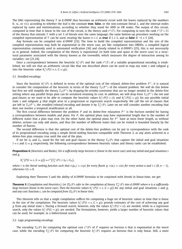
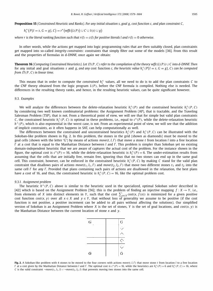
certain atoms are dropped from the problem [29,37]). Using this technique, we were able to compile theories with up to 10floors and 10 positions in less than a second. The problem in Fig. 1 is then solved optimally in milliseconds, expanding 65nodes. As a reference, a ‘blind’ search based on the non-informative admissible heuristic h0 that adds up all the uncollectedrewards, takes 27 seconds and expands 445,956 nodes. More results appear in Table 5 where it is shown that the heuristicis cost-effective in this case, and enables the optimal solution of problems that are not trivial.
B. Bonet, H. Geffner / Artificial Intelligence 172 (2008) 1579–1604 1593
Table 5Search results for Elevator with h0 and relaxed h+
c heuristics. Instance n-m-k refers to a problem with n floors, m positions and k elevators. Probleminstance and its optimal cost are shown, and for h0 and h+
c , the value of the heuristic at the initial state, the length of the optimal plan, the number ofexpanded nodes, and the search time in seconds. A dash means that the search did not finish within the limits of 2 hours and 2 Gb of memory
Problem c∗(P ) h0 backward with mutex relaxed h+c backward with mutex
h0(P ) len nodes time relaxed h+c (P ) len nodes time
4-4-2 −1 −14 6 3399 0.0 −3 6 15 0.06-6-2 −6 −28 15 67,722 3.5 −13 15 499 0.06-6-3 −6 −28 15 472,446 31.7 −15 15 2505 0.610-5-1 −3 −42 11 445,956 27.0 −6 11 65 0.010-5-2 −5 −42 – – – −21 32 66,486 16.710-10-2 −7 −63 – – – −22 23 194,069 109.6
9. Boosting the heuristic: Plan constraints
The formulation of the delete-based relaxation heuristic in logic along with its computational model based on a compiledd-DNNF formula, can be extended in a natural way to a more powerful class of heuristics that are not bound by thelimitations of the delete-relaxation. We consider one particular extension that results from taking constraints on plans intoaccount: these are constraints over the sets of actions and fluents that are allowed in a plan: plans that violate suchconstraints will be ruled out by assigning them infinite cost. We will be interested in plan constraints that are valid in aproblem in the sense that they are satisfied by some optimal plan. Making such constraints explicit has no effect on theoptimal cost of a problem but will boost the heuristic function that is obtained from it by capturing information that is lost inthe delete relaxation. For example, for suitable plan constraints, the new heuristic will be optimal for the Traveling SalesmanProblem (TSP), where the delete-relaxation heuristic h+
c , which is also exponential in the worst case (unless P = NP), yieldsthe poorer Minimum Spanning Tree (MST) lower bound.
9.1. Syntax and semantics
A plan constraint C is a propositional formula over the sets of actions and fluents A and F . A plan π for a problem Psatisfies a constraint C , written π | C , if C is true over the interpretation that makes true only the actions and fluents inπ and F (π); i.e.
π | C for C ∈ A ∪ F iff C ∈ π or C ∈ F (π),
π | ¬C iff π �| C,
π | C ∨ C ′ iff π | C or π | C ′,
π | C ∧ C ′ iff π | C and π | C ′.
Intuitively, a constraint p ∨ q when p and q are fluents is satisfied by π when π makes p or q true at some point in theexecution. Similarly, a constraint ¬p ∨ ¬q is satisfied when p, q, or both, are never made true by π . These plan constraintsthus, should not be confused with the mutex constraints (p,q) [11] that express a constraint over the truth of p and q atthe same time point. Plan constraints as defined are not as expressive as modal or temporal formulas, but are simple andsufficient for illustrating how the basic delete-relaxation heuristic can be improved.
Plan constraints are not used to modify the definition of plans but rather their costs, so that plans that do not complywith the constraints get an infinite cost:
Definition 10 (Constrained Plan Costs). The constrained cost c(π, C) of a plan π for a planning problem P extended with a setof plan constraints C is
c(π, C)def=
{c(π) if π | C
∞ otherwise.(14)
Definition 11 (Constrained Costs). The constrained optimal cost c∗(P , C) is
c∗(P , C)def= min
πc(π, C) (15)
where π ranges over the plans for P , and c∗(P , C) = ∞ if no plan for P satisfies C .
Plan constraints increase the expressive power of the planning language, yet we are interested in plan constraints thatare implicit in the sense that they have no effect on the cost of a problem:

1594 B. Bonet, H. Geffner / Artificial Intelligence 172 (2008) 1579–1604
Definition 12 (Valid Plan Constraints). A plan constraint C is implicit or valid in a problem P under a given cost function cwhen C is satisfied by some optimal plan if the problem admits a plan at all.
Clearly if C is a valid constraint for problem P under the cost function c, c∗(P , C) = c∗(P ). A sufficient condition for Cto be valid for P under any cost function is when C is satisfied by all plans for P , whether optimal or not. For example, theconstraint that prevents two moves away from the same city is true in all ‘plans’ that solve the Traveling Salesman Problem.On the other hand, the constraint that no block needs to be unstacked from two different blocks is a valid constraint in theBlocks World under the classical 0/1 cost function, but is not true in all plans and not even in all optimal plans (e.g., anoptimal plan that moves a block to the table and then moves this block to its target destination can often be transformedinto an optimal plan where the block is first moved on top of an irrelevant block instead).
The key point is that while valid plan constraints C do not affect the optimal cost of a problem P , they can potentiallyincrease the value of the delete-relaxation heuristic:
Definition 13 (Constrained Heuristic). The constrained delete-relaxation heuristic of a planning problem P extended with theplan constraints C is defined as
h+c (P , C)
def= c∗(P+, C) (16)
where P+ is the delete-relaxation of P .
The constrained delete-relaxation heuristic h+c (P , C) can be more informed than the plain delete-relaxation heuristic
h+c (P ) while remaining a lower bound on the true cost c∗(P ):
Theorem 14 (Admissibility and Boosting). Let C be a plan constraint that is valid in P under the cost function c. Then,
h+c (P ) � h+
c (P , C) � c∗(P , C) = c∗(P ),
where the two inequalities can be strict.
The first inequality h+c (P ) � h+
c (P , C) is direct and is always true as the second heuristic simply pushes the cost of someplans π in the relaxation P+ to infinite, while the equality c∗(P , C) = c∗(P ) is true from the validity of C . The heuristicvalue can only increase from h+
c (P ) to h+c (P , C) when C is a constraint valid in P but invalid in the delete-relaxation P+ .
Theorem 14 is important as it says that the value of the delete-relaxation heuristic h+c can be increased, while preserving
admissibility, by simply making explicit certain valid but implicit plan constraints. Before showing how to account forthe new heuristic h+
c (P , C) in the semantic and computational framework laid out above for h+c (P ), let us illustrate the
difference between the two heuristics over a concrete example.
Consider a problem P where an agent, initially at location L, has to pick up a package p at location L′ and return back toL with the package. If the available actions allow the agent to move from one location to the other, and pick up a packageif at the same location as the package, then a plan like
move(L, L′),pick(p, L′),move(L′, L)
is optimal for a cost c∗(P ) = 3. The optimal cost of the relaxation P+ , on the other hand, is c∗(P+) = 2 as in the absenceof deletes, the last action move(L′, L) is not needed in order to return to L. This means that the delete-relaxation heuristich+
c (P ) is 2 as well.Consider now the constraint C : move(L, L′) ⊃ move(L′, L). This constraint is valid in P : if the agent moves away from
the goal location then it has to get back to it. The delete-relaxation heuristic constrained with C can be shown to beh+
c (P , C) = c∗(P+, C) = 3, and hence strictly greater than the normal delete-relaxation heuristic h+c (P ) = c∗(P+) = 2. This
is because while any plan for P+ must include the actions move(L, L′) and pick(p, L′), the constraint C forces the actionmove(L′, L) to be in the plan too.
The example shows that the value of the delete-relaxation heuristic h+c (P ) can be boosted by making explicit certain
constraints that are otherwise implicit. We do not consider in this paper the problem of deriving or learning such constraintsautomatically. Our goal instead is to show that such constraints can be naturally incorporated in the framework presentedand that they can make a significant difference in relation to heuristics that are based on the delete-relaxation only.
9.2. Logical formulation and computation
Proposition 6 established the relation between the heuristic value h+c (P [I = s, G = g]), for any initial state s and goal
g , and the rank r∗(wffc(L(P )) ∪ I(s) ∪ g) of the propositional theory obtained from the logic program L(P ) encoding therelaxation P+ of P , and the literals I(s) ∪ g encoding the state s and goal g . The extension of this correspondence in thepresence of plan constraints C is straightforward:
B. Bonet, H. Geffner / Artificial Intelligence 172 (2008) 1579–1604 1595
Proposition 15 (Constrained Heuristic and Ranks). For any initial situation s, goal g, cost function c, and plan constraint C ,
h+c
(P [I = s, G = g], C
) = r∗(wffc(L(P )
) ∪ C ∪ I(s) ∪ g)
where r is the literal ranking function such that r(l) = c(l) for positive literals l and r(l) = 0 otherwise.
In other words, while the actions get mapped into logic programming rules that are then suitably closed, plan constraintsget mapped into so-called integrity constraints: constraints that simply filter out some of the models [36]. From this resultand the properties of formulas in d-DNNF, once again we obtain:
Theorem 16 (Computing Constrained Heuristics). Let Π(P , C) refer to the compilation of the theory wffc(L(P ))∪ C into d-DNNF. Thenfor any initial and goal situations s and g, and any cost function c, the heuristic value h+
c (P [I = s, G = g], C) can be computedfrom Π(P , C) in linear time.
This means that in order to compute the constrained h+c values, all we need to do is to add the plan constraints C to
the CNF theory obtained from the logic program L(P ), before the CNF formula is compiled. Nothing else is needed. Thedifferences in the resulting theory ranks, and hence, in the resulting heuristic values, can be quite significant however.
9.3. Examples
We will analyze the differences between the delete-relaxation heuristic h+c (P ) and the constrained heuristic h+
c (P , C)
by considering two well known combinatorial problems: the Assignment Problem (AP), that is tractable, and the TravelingSalesman Problem (TSP), that is not. From a theoretical point of view, we will see that for simple but valid plan constraintsC , the constrained heuristic h+
c (P , C) is optimal in these problems, i.e., equal to c∗(P ), while the delete-relaxation heuristich+(P ), which is also exponential in the worst case, is not. From an experimental point of view, we will see that the additionof implicit constraints, as it often happens in SAT, can help computationally as well.
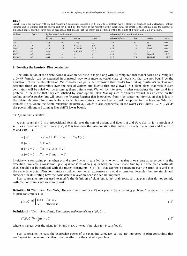
The differences between the constrained and unconstrained heuristics h+c (P ) and h+
c (P , C) can be illustrated with theSokoban-like problem shown in Fig. 2. In this problem, the stones in the grid (shown as diamonds) must be moved to thegoal cells (shown with the letter ‘G’) by means of actions move(t, l, l′) that move a stone t from location l into a free locationl′ at a cost that is equal to the Manhattan Distance between l and l′ . This problem is simpler than Sokoban yet no existingdomain-independent heuristic that we are aware of captures the actual cost of the problem. For the instance shown in thefigure, the optimal cost is c∗(P ) = 16, while the delete-relaxation heuristic is h+
c (P ) = 6. The under-estimation results fromassuming that the cells that are initially free, remain free, ignoring thus that no two stones can end up in the same goalcell. This constraint, however, can be enforced in the constrained heuristic h+
c (P , C) by making C stand for the valid planconstraint that disallows pairs of actions move(t1, l1, l′) and move(t2, l2, l′) that move two different stones t1 and t2 into thesame cell l′ for any l′ . Provided that plans containing such pairs of actions are disallowed in the relaxation, the best planshave a cost of 16, and thus, the constrained heuristic is h+
c (P , C) = 16, like the optimal problem cost.
9.3.1. Assignment problemThe heuristic h+(P , C) above is similar to the heuristic used in the specialized, optimal Sokoban solver described in
[42] which is based on the Assignment Problem [56]; this is the problem of finding an injective mapping f : X → Y , i.e.,from elements of X into distinct elements in Y , such that the cost
∑x∈X cost(x, f (x)) is minimized for a given positive
cost function cost(x, y) over all x ∈ X and y ∈ Y , that without loss of generality we assume to be positive (if the costfunction is not positive, a positive increment can be added to all pairs without affecting the solutions). Our simplifiedversion of Sokoban is an Assignment Problem where X is the set of stones, Y is the set of goal locations, and cost(x, y) isthe Manhattan Distance between the current location of stone x and y.
Fig. 2. A Sokoban-like problem with 4 stones to be moved to the four corners with actions move(t, l, l′) that move stone t from location l to a free locationl′ at a cost given by the Manhattan Distance between l and l′ . The optimal cost is c∗(P ) = 16, while the heuristics are h+
c (P ) = 6 and h+c (P , C) = 16, where
C is the valid constraint ¬move(t1, l1, l) ∨ ¬move(t2, l2, l) that prevents moving two stones into the same cell.
1596 B. Bonet, H. Geffner / Artificial Intelligence 172 (2008) 1579–1604
Any such assignment problem can be formulated into a planning problem through an encoding with fluents
assigned(x), free(y)
for each x ∈ X and y ∈ Y , and actions map(x, y) with precondition, add, and delete lists
P : free(y); A : assigned(x); D : free(y).
Initially, free(y) is true for all y ∈ Y , while assigned(x) must be true for all x ∈ X in the goal.It is easy to show that each plan of the resulting encoding corresponds to an assignment and that, for the cost function
c(map(x, y)) = cost(x, y), the optimal plans corresponds to the optimal assignments. Furthermore, by making explicit thevalid plan constraint C
¬map(x, y) ∨ ¬map(x′, y)
for all y ∈ Y and x, x′ ∈ X such that x �= x′ (not two x’s mapped into the same y), the heuristic h+c (P , C) is optimal.
Theorem 17 (Assignment Problem). Let P be the planning problem encoding an arbitrary assignment problem, and let C be the validplan constraint that prevents assigning two domain elements to the same target element. Then, the heuristic h+
c (P , C) is optimal; i.e.,h+
c (P , C) is equal to the cost of the optimal assignment.
The delete-relaxation heuristic h+c (P ), on the other hand, is not optimal and may not even reflect the cost of any as-
signment. Indeed, while h+c (P , C) yields the minimum of
∑x∈X cost(x, f (x)) over all the injective (one-to-one) functions
f : X → Y , h+c (P ) yields the minimum over all functions f : X → Y , injective or not.
This class of problems shows that valid plan constraints can be used for capturing structural information that is lostin the delete-relaxation without the need for bringing time indices back in the formulation. We will show that the samehappens in another combinatorial problem that unlike the Assignment Problem is intractable.
9.3.2. The Traveling Salesman problemWe consider now a problem harder than the Assignment Problem: the Traveling Salesman Problem (TSP), a well-known
combinatorial problem that surfaces in a number of applications and is known to be intractable [56]. Once again we willencode the TSP as a planning problem, and prove that for simple valid plan constraints C , the constrained heuristic h+
c (P , C)
is optimal while the unconstrained heuristic h+c (P ), which is also exponential in the worst case, is not. Moreover, we will
show that the latter captures the Minimum Spanning Tree (MST) lower bound, which unlike the TSP can be solved efficiently[56].
The TSP is the problem of finding a minimum cost tour in a given directed graph G = (V , E) extended with cost infor-mation c(x, y) on the edges (x, y) ∈ E which we assume to be positive (else positive increments can be added to all edgeswithout affecting the solutions). A tour is a path that starts and ends in the same vertex, visiting all other vertices in thegraph exactly once. The TSP problem can be encoded as a planning problem with the fluents
at(x), visited(x), not-visited(x),
for x ∈ V ′ , where V ′ = V ∪ {x f } and x f is an additional, dummy vertex that stands for a copy of the first vertex x0 in thetour, chosen arbitrarily from V . The actions move(x, y) for x ∈ V , y ∈ V ′ and x �= y, have precondition, add, and delete lists
P : at(x),not-visited(y); A : at(y),visited(y); D : at(x),not-visited(y).
The action costs c(move(x, y)) must be set to cost(x, y) if (x, y) ∈ E and y �= x f , to cost(x, x0) if y = x f and (x, x0) ∈ E , to0 if x = x0 and y = x f , and to ∞ otherwise. If the graph is sparse a more compact encoding results from using the set ofedges E to exclude actions move(x, y) when (x, y) is not in E . The theoretical results, however, apply to either encoding.Finally, the initial situation must be set to the atoms at(x0), visited(x0), not-visited(y) for all y ∈ V ′ , y �= x0, while the goalsituation must be set to visited(y) for all y ∈ V ′ .
It is easy to show that this encoding is correct; namely that if (x0, x1, . . . , xn, x0) is an optimal solution of a TSP, theaction sequence 〈move(x0, x1) . . . ,move(xn, x f )〉 is an optimal solution with the same cost in the corresponding planningproblem. More interestingly, we can prove that the heuristic h+
c (P , C) is optimal provided that C is the constraint that rulesout two moves away from the same vertex:
Theorem 18 (Optimality of Constrained h+c for TSP). Let T be a TSP, P and c stand for its planning encoding, and let C stand for the
valid plan constraint
¬move(x, y) ∨ ¬move(x, y′)
over the actions in P for all x and y �= y′ . Then, the heuristic h+c (P , C) is optimal; i.e., h+
c (P , C) is equal to the cost of the optimal TSPsolution.
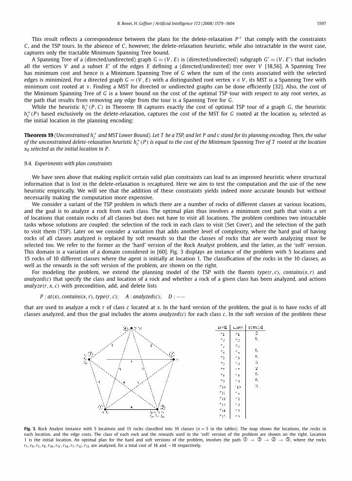
B. Bonet, H. Geffner / Artificial Intelligence 172 (2008) 1579–1604 1597
This result reflects a correspondence between the plans for the delete-relaxation P+ that comply with the constraintsC , and the TSP tours. In the absence of C , however, the delete-relaxation heuristic, while also intractable in the worst case,captures only the tractable Minimum Spanning Tree bound.
A Spanning Tree of a (directed/undirected) graph G = (V , E) is (directed/undirected) subgraph G ′ = (V , E ′) that includesall the vertices V and a subset E ′ of the edges E defining a (directed/undirected) tree over V [18,56]. A Spanning Treehas minimum cost and hence is a Minimum Spanning Tree of G when the sum of the costs associated with the selectededges is minimized. For a directed graph G = (V , E) with a distinguished root vertex v ∈ V , its MST is a Spanning Tree withminimum cost rooted at v . Finding a MST for directed or undirected graphs can be done efficiently [32]. Also, the cost ofthe Minimum Spanning Tree of G is a lower bound on the cost of the optimal TSP tour with respect to any root vertex, asthe path that results from removing any edge from the tour is a Spanning Tree for G .
While the heuristic h+c (P , C) in Theorem 18 captures exactly the cost of optimal TSP tour of a graph G , the heuristic
h+c (P ) based exclusively on the delete-relaxation, captures the cost of the MST for G rooted at the location x0 selected as
the initial location in the planning encoding:
Theorem 19 (Unconstrained h+c and MST Lower Bound). Let T be a TSP, and let P and c stand for its planning encoding. Then, the value
of the unconstrained delete-relaxation heuristic h+c (P ) is equal to the cost of the Minimum Spanning Tree of T rooted at the location
x0 selected as the initial location in P .
9.4. Experiments with plan constraints
We have seen above that making explicit certain valid plan constraints can lead to an improved heuristic where structuralinformation that is lost in the delete-relaxation is recaptured. Here we aim to test the computation and the use of the newheuristic empirically. We will see that the addition of these constraints yields indeed more accurate bounds but withoutnecessarily making the computation more expensive.
We consider a variant of the TSP problem in which there are a number of rocks of different classes at various locations,and the goal is to analyze a rock from each class. The optimal plan thus involves a minimum cost path that visits a setof locations that contain rocks of all classes but does not have to visit all locations. The problem combines two intractabletasks whose solutions are coupled: the selection of the rock in each class to visit (Set Cover), and the selection of the pathto visit them (TSP). Later on we consider a variation that adds another level of complexity, where the hard goal of havingrocks of all classes analyzed is replaced by soft rewards so that the classes of rocks that are worth analyzing must beselected too. We refer to the former as the ‘hard’ version of the Rock Analyst problem, and the latter, as the ‘soft’ version.This domain is a variation of a domain considered in [60]. Fig. 3 displays an instance of the problem with 5 locations and15 rocks of 10 different classes where the agent is initially at location 1. The classification of the rocks in the 10 classes, aswell as the rewards in the soft version of the problem, are shown on the right.
For modeling the problem, we extend the planning model of the TSP with the fluents type(r, c), contains(x, r) andanalyzed(c) that specify the class and location of a rock and whether a rock of a given class has been analyzed, and actionsanalyze(r, x, c) with precondition, add, and delete lists
P : at(x), contains(x, r), type(r, c); A : analyzed(c); D : −−that are used to analyze a rock r of class c located at x. In the hard version of the problem, the goal is to have rocks of allclasses analyzed, and thus the goal includes the atoms analyzed(c) for each class c. In the soft version of the problem these
Fig. 3. Rock Analyst instance with 5 locations and 15 rocks classified into 10 classes (n = 5 in the tables). The map shows the locations, the rocks ineach location, and the edge costs. The class of each rock and the rewards used in the ’soft’ version of the problem are shown on the right. Location1 is the initial location. An optimal plan for the hard and soft versions of the problem, involves the path 1! → 3! → 2! → 5!, where the rocksr1, r9, r5, r8, r10, r11, r14, r7, r12, r13 are analyzed, for a total cost of 18 and −18 respectively.

1598 B. Bonet, H. Geffner / Artificial Intelligence 172 (2008) 1579–1604
Table 6Compilation results for Rock Analyst with hard goals: problem instance and optimal costs shown along with the value of the heuristic at the initial state,and the time to compute the heuristic h2 and h+
c with and without the constraint C that rules out two moves away from the same location. For theheuristics h+
c , the size of the compilation in bytes is also shown. A dash means the theory did not compile within the limits of 1 hour and 1 Gb of memory
n c∗(P ) h2 h+c unconstrained h+
c constrained
h2(P ) time h+c (P ) time size h+
c (P , C) time size
4 13 7 0.2 12 0.0 2.2K 13 0.0 3.2K5 18 10 0.8 17 0.0 9.2K 18 0.0 12K6 18 6 2.1 18 0.1 56K 18 0.2 65K7 22 8 5.0 21 1.3 587K 22 1.4 392K8 23 7 10.6 22 18.3 6.3M 23 16.3 3.9M9 26 8 20.7 25 367.6 73M 26 1217.7 22M10 29 7 37.9 – – – – – –11 31 7 65.9 – – – – – –12 – 7 107.6 – – – – – –
atoms are given positive rewards (negative costs). We consider random problems with n locations, 2n non-empty classes,and 3n rocks, for n = 4,5, . . . ,12.
Table 6 shows the compilation results for the ‘hard’ version of the problem where rocks of all classes must be analyzed.The table displays the costs of the optimal tour, the values of the heuristics h+
c (P ) and h+c (P , C), where C is the constraint
that prevents two moves away from the same location,10 and the time and size of the compilation in d-DNNF. In addition, asa reference, the value of the h2 heuristic [39], along with the time for computing the heuristic for all atom pairs is reportedtoo. As it can be seen from the table, the theory with constraints results in optimal heuristic values h+
c (P , C) = c∗(P ),while the theory without constraints gives lower bounds h+
c (P ) � c∗(P ), which in these instances are quite accurate. Thecompilation of the theory with and without constraints scales up only up to the problem with the number of locationsn = 9, with the former producing smaller d-DNNF formula although not always in less time. The heuristic h2, on the otherhand, is quadratic and scales up to larger problems, although is not well informed, and results in a search that explores anexponentially larger number of nodes.
Table 7 shows the results of a regression search guided by these three heuristics. The search algorithm, as before, is A∗with the revised termination condition that ensures optimality in the presence of negative costs and a monotone heuristic.11
The three heuristics are extended with structurally mutex information so that states in the regression that include anunreachable atom pair are immediately pruned. Not surprisingly, the search with the constrained heuristic h+
c (P [G = g], C)
yields the best results with the least number of expanded nodes. Yet, once the compilation effort is taken into account,the standard h2 heuristic is best, managing to solve the instances with n = 10 and n = 11 that the other two heuristicscannot solve, even if they expand a much lower number of nodes. In each of the cases, the table shows also the lengthsof the optimal plans found; all these plans must have the same (optimal) cost but do not have to have the same length.It should be noted that while the heuristic h+
c (P [G = g], C) is optimal in this problem when g is the top goal, it is notnecessarily optimal over all the subgoals g′ that arise in the regression. This explains why the number of nodes expandedby the heuristic in the regression is sometimes larger than the number of actions in the optimal plan.
We also considered a ‘soft’ version of the problem where the fluents analyzed(c) are removed from the goal and are givenrewards (negative costs) randomly chosen between [−6,−1]. Table 8 shows the results for the compilation. Once again, theconstraints improve the size of the compilation, although not necessarily the time. The heuristic used as a reference is theheuristic h0 that is also admissible and simply adds up all the uncollected rewards. The heuristic values h0(P ) are muchless informed than h+
c (P ) and h+c (P , C) but much cheaper to compute.
Table 9 shows the results of the search. In this case, h+c (P ) and h+
c (P , C) do best, with the latter expanding a smallernumber of nodes in less time. The heuristic h0, as the heuristic h2 in the ‘hard’ version of the problem, requires an expo-nentially larger number of nodes to be explored scaling up to problems with n = 7. The other two heuristics scale up withthe compilation until n = 9.
10 This constraint is valid provided that all locations are connected and that the direct path between any two locations is not more costly than an indirectpath. These two conditions are true in the problems below.11 The search for optimal plans using the heuristic function h+
c extended with a set of constraints C raises two additional issues that need to be addressedthat we mention briefly here. First, for the heuristic to remain consistent during the search with constraints, search nodes must become triplets n = 〈s, t, v〉,where s and t stand as before for the progressed state and the set of atoms p encountered in the path to n from the root with cost c(p) �= 0, and the newcomponent v is the set of atoms p encountered along the same path that occur in C . The heuristic h(n) of the node n is then h+
ct(P [I = s], C v ), where
ct is a cost function like c but with c(p) = 0 if p ∈ t , and C v is a constraint like C but with p replaced by the boolean true (a similar representation isneeded for a regression search). Second, since the compilation of the theory wffc(L(P )) ∪ C ensures that the heuristic values h+
c (P [I = s, G = g], C) can becomputed in linear time for any state s, subgoal g , and cost function c, but not for any constraint C , in order to compute h(n) = h+
ct(P [I = s], C v ) in linear
time for any n = 〈s, t, v〉, a theory wffc(L(P )) ∪ C ′ slightly different than wffc(L(P )) ∪ C needs to be compiled, where C ′ is C but with all its variables xreplaced by copies x′ , along with the implications x ⊃ x′ . We omit the details and proofs of these extensions that are implemented in the planner.

B. Bonet, H. Geffner / Artificial Intelligence 172 (2008) 1579–1604 1599
Table 7Search results for Rock Analyst with hard goals: problem instance and optimal cost shown, along with the plan length, number of nodes expanded, andplan time in seconds, for the heuristics h2 and h+
c with and without the constraint C . A dash means that the search did not finish within the limits of1 hour and 2 Gb of memory
n c∗(P ) h2 h+ unconstrained h+c constrained
len nodes time len nodes time len nodes time
4 13 11 190 0.0 11 43 0.0 11 12 0.05 18 14 1982 0.0 14 161 0.0 13 13 0.06 18 16 5901 0.2 16 191 0.0 16 79 0.07 22 19 26,548 1.6 19 283 0.9 19 19 0.08 23 22 75,758 5.7 22 456 43.2 22 38 3.69 26 24 452,155 46.3 23 667 729.2 23 23 18.810 29 27 1,612,766 197.6 – – – – – –11 31 30 4,213,661 620.8 – – – – – –12 – – – – – – – – – –
Table 8Compilation results for Rock Analyst with soft goals: problem instance and optimal cost shown along with the value of the heuristic at the initial statewith the time in seconds needed to compute the heuristic h0 (sum of uncollected rewards) and h+
c with and without the valid constraint C that rules twomoves away from the same location. For the heuristics h+
c , the size of the compilation in bytes is also shown. A dash means the theory did not compilewithin the limits of 1 hour and 1 Gb of memory
n c∗ h0 h+c unconstrained h+
c constrained
h0(s0) time h+c (P ) time size h+
c (P , C) time size
4 −5 −18 0.0 −6 0.0 2.2K −5 0.0 3.2K5 −18 −36 0.0 −19 0.0 9.2K −18 0.0 12K6 −19 −37 0.0 −19 0.1 56K −19 0.2 65K7 −19 −40 0.0 −20 1.3 587K −19 1.4 392K8 −25 −48 0.0 −26 18.2 6.3M −25 16.4 3.9M9 −19 −44 0.0 −19 366.7 73M −19 910.3 23M10 – −54 0.0 – – – – – –11 – −76 0.0 – – – – – –12 – −64 0.0 – – – – – –
Table 9Search results for Rock Analyst with soft goals: problem instance and optimal cost shown, along with the plan length, number of nodes expanded, and plantime in seconds, for the heuristics h0 and h+
c with and without the constraint C . A dash means that the search did not finish within the limits of 1 hourand 2 Gb of memory
n c∗(P ) h0 h+c unconstrained h+
c constrained
len nodes time len nodes time len nodes time
4 −5 4 7959 0.3 8 53 0.0 4 5 0.05 −18 11 119,729 7.3 14 168 0.0 13 13 0.06 −19 13 1,461,436 168.9 14 461 0.3 14 77 0.17 −19 12 8,175,484 1363.7 17 131 1.2 17 33 0.28 −25 – – – 21 1653 262.5 20 36 7.99 −19 – – – 19 168 611.4 19 19 35.310 – – – – – – – – – –11 – – – – – – – – – –12 – – – – – – – – – –
10. Discussion
In this work we have used propositional logic in various forms (CNF, Logic Programs, d-DNNF), for defining admissibleheuristic for planning in the presence of costs and rewards that are computed by means of circuits that map situations intovalues in time that is linear in the circuit size. This circuit is a simple transformation of the d-DNNF formula encoding thedomain where ANDs and ORs are replaced by Adders and Min Operators, and whose output for any situation encodes thecost of the best model. In the worst case, the d-DNNF formula, and hence the evaluation circuit, can have a size that isexponential in the treewidth of the CNF encoding [21]. While this is a worst-case bound and the experiments show thata number of non-trivial problems can be solved by heuristics defined and computed in this way, it nonetheless expressesthe practical limitation of the formulation in its current form. A possible way to overcome this limitation is the use ofadditional relaxations able to map CNF theories into weaker theories of bounded treewidth that can be then compiled inpolynomial time and space. This is the approach we have taken recently in [58] for solving MinCostSAT problems. This typeof relaxation in a planning setting results in a family of tractable, admissible heuristics, computable by circuits, that captureinformation about the delete lists in the problem in the form of valid plan constraints. Preliminary experiments using theseheuristics are reported in [57].

1600 B. Bonet, H. Geffner / Artificial Intelligence 172 (2008) 1579–1604
The effective use of propositional logic in classical planning has been championed by Kautz and Selman in [43–45],where Strips problems P are mapped into CNF theories T (n) for a planning horizon n that are fed into state-of-the-art SATsolvers. The encoding ensures a correspondence between the logical models of T (n) and the plans for P . A similar approachbut in the context of Logic Programming, has been proposed in [27,46,62] where CNF encodings of planning problemsare replaced by Logic Programs whose Answer Sets, computed by state-of-the-art ASP Solvers, are in correspondence withthe target plans. Logic programs allow for more concise encodings although this does not translate necessarily into fastersolutions due to speed of current SAT solvers.
The differences between our use of logic for planning and these other approaches are basically three. First, we use logicfor defining and computing heuristics for planning, not for computing the plans themselves. This allows us to use morecompact encodings that do not require time indices or planning horizons. This is important because, the complexity of theencodings grows exponentially with the horizon, and except for the plan metric defined by the horizon, the optimality ofthe plans obtained is conditional on the horizon used.
Second, the resulting logical encoding is not solved using a SAT or ASP solver, but using a d-DNNF compiler. Once theproblem is compiled, the heuristic values for any search state are found in time that is linear in the compiled representation.Incidentally, the d-DNNF compiler can be thought of as a SAT solver with a suitable form of caching that computes allsolutions and leaves a ‘trace’ behind that enables the solution of other problems as well [38]. Another use of d-DNNFin planning is reported in [54], where heuristics for planning under incomplete information and no sensing (conformantplanning) are obtained using projections and model counts computable in linear-time over d-DNNF representations [25].
Third, the heuristics handle a richer cost structure where actions can have non-uniform costs, and penalties and rewardsmay be associated with fluents. The computation of optimal plans in rich cost structures has been pursued recently in [8,30,35] where planning problems are mapped into optimization variants of SAT, Answer Sets, or CSPs (Constraint SatisfactionProblems) like Weighted Max-SAT, Weighted ASP, and Weighted CSPs. A serious limitation of these approaches, however, isthat the optimality of the resulting plans is conditional on the horizon used. Moreover, increasing the planning horizon oneby one is no alternative because it is not clear when to stop, as plans with a larger makespan can potentially decrease theoverall cost.
Approaches for planning with preferences in the form of soft goals are reported in [7,60,64]. The latter two approaches,however, are not optimal for various reasons: in some cases, heuristic mechanisms are used to select the soft goals topursue, in others, a fixed planning horizon is assumed, and finally in others, a suboptimal Anytime A∗ search algorithm isused. The work in [7], on the other hand, presents an optimal planner for dealing with temporally extended preferencesbased on a branch-and-bound search, yet the lower bounds utilized are not sufficiently informed, and thus the search cannotbe run to completion in general.
The problems of selecting a subset of the soft goals to pursue along with the estimation of the cost for achieving themare tightly coupled. The heuristics developed in this paper tackle them both at the same time: the best model of the theoryselects the ‘soft goals’ that are to be pursued at the same time that it estimates the cost of achieving them. The heuristic isindeed optimal for this task when there are no deletes.
11. Summary
We have combined ideas from a number of areas, including search, planning, knowledge compilation, and answer setprogramming to develop
1. a cost model for planning that accommodates fluent penalties and rewards,2. a generalization of the admissible delete-relaxation heuristic h+
c for informing the search in the model,3. an account of the heuristic in terms of the rank of the best models of a suitable propositional theory obtained from the
strong completion of a logic program that does not require time indices or horizons,4. an approach that exploits this formulation along with the properties of d-DNNF formula for computing all heuristic
values h+c needed in the search in time linear in the size of the compilation,
5. a best-first algorithm able to use this heuristic, capable of handling negative heuristics and costs while ensuring opti-mality, and
6. an extension of the framework based on the use of valid plan constraints for boosting the values of the heuristic,overcoming some of the limitations of the delete-based relaxation.
We have also analyzed some of the properties of the resulting heuristics such as admissibility and monotonicity, as wellas some of the semantic differences between the heuristic h+
c (P ) and constrained heuristic h+c (P , C), showing for example
that the latter produces optimal costs in problems such as the Traveling Salesman Problem where the former yields only theMinimum Spanning Tree lower bound, even if both heuristics are exponential in the worst case. We have also implementedthese ideas in a planner that we tested on a number of problems, producing non-trivial results, including the best resultswe are aware of in some domains.
The computational bottleneck in this approach is the compilation of the CNF translation of the logic program into ad-DNNF formula. In [58] and [57], we report preliminary results of an additional relaxation method that maps the CNFformula into a weaker formula of bounded treewidth that can be compiled efficiently.

B. Bonet, H. Geffner / Artificial Intelligence 172 (2008) 1579–1604 1601
The results above do not have to be taken as a single package, and in particular it is possible to replace the compilationstep by an explicit computation of the best models for each of the states that arise in the search, using a Weighted SATor ASP solver. The appeal of the compilation-based approach, however, is that it yields what can be deemed as a circuit orevaluation network whose input is a situation and whose output, produced in linear-time, is an appraisal of the situation inthe form of its heuristic value. Some authors have associated evaluations of this type with the role played by emotions inreal agents [20,28].
Acknowledgements
We thank Adnan Darwiche for useful discussions about d-DNNF and for making his compiler available, and the anony-mous reviewers for useful comments. H. Geffner is partially supported by grant TIN2006-15387-C03-03 from MEC/Spainand B. Bonet by a grant from DID/USB/Venezuela. Our planner was built upon a planner by Patrik Haslum. Preliminaryexperiments were run on the Hermes Computing Resource at the Aragon Institute of Engineering Research (I3A), Universityof Zaragoza.
Appendix A. Proofs
We include proofs of the results in the paper whose derivation is not direct from the text.
Proof of Proposition 1. Any plan π for P is a plan for the relaxation P+ as well, and if F (π) and F +(π) stand for the setof atoms made true by π in P and in P+ respectively, clearly F (π) = F +(π). It follows then that any plan π in P is a planfor the relaxation P+ with the same cost, and hence that h+
c (P ) = c∗(P+) cannot be higher than c∗(P ). �Proof of Proposition 2. The correspondence between the plans of length n and the models of Tn(P ) for a sufficiently largen is established in [44]. In the worst case, this horizon can be exponential [15]. �Proof of Proposition 4. The proposition follows from the correspondence between the models of T +
n (P ) ∪ I0 ∪ Gn and theplans for P+[I = s, G = g]. The models M of T +
n (P ) ∪ I0 ∪ Gn are in 1–1 correspondence with the plans π for P+[I = s, G =g] for a sufficiently large n. Moreover, for the literal-ranking function given in the proposition, r(M) = c(π), as if the actiona occurs at time i in the plan, then ai is true in the model, and hence the contribution of this action to c(π) and r(M) isthe same. In addition, if a fluent p is made true by the plan at any one point, due to the absence of deletes, p must be truetoo at the end of the plan, and hence pn must be true in the model. Since r(pn) = c(p), fluents also contribute the sameterms to both c(π) and r(M). �Proof of Proposition 6. We establish a correspondence between the plans π for the P+([I = s, G = g]) and the models ofwffc(L(P ))∪ I(s)∪ g . An interpretation over the theory T = wffc(L(P ))∪ I(s)∪ g can be expressed as a pair (A, F ) of actionsA and fluents F . Moreover, in the models (A, F ) of wffc(L(P )), the set of fluents F is determined by the set of actions A asfrom the definition of wffc(L(P )), F is the unique minimal model of the logic program L(P ) ∪ A. The set of fluents F thatare true in such a model, that we call F (A), can be stratified into sets F0(A), F1(A), . . . , where F0(A) contains the heads pof rules p ← Pre(a),a in L(P ) such that a ∈ A and Pre(a) is empty, while Fi+1(A) contains the heads of the same rules witha ∈ A and Pre(a) becoming true at i (Pre(a) becomes true at i if some q ∈ Pre(a) is in Fi(A), and the other atoms r ∈ Pre(a),if any, are in Fk(A), for k � i).
Now, if (A, F ) is a best model of T such that for some actions a ∈ A, their preconditions are not all true in F , byconstruction of L(P ) and since c(a) � 0 it is possible to construct another model (A′, F ) of T , A′ ⊂ A, with these actionseliminated and with the same set of fluents, that is as good as (A, F ) and where all preconditions are satisfied. We wantto show that such a model (A′, F ) encodes a ‘parallel’ plan π for P+([I = s, G = g]) with the same cost. In the delete-relaxation, any parallel Strips plan can be serialized, keeping its cost, and also, any sequential plan can be parallelized bymoving the actions to the first time point where its preconditions hold. The parallel plan π that corresponds to (A′, F ) isdefined as the sequence of action sets A0, A1, . . . where Ai is the set of actions in A′ whose preconditions become true at iin F (A′), with the ‘set actions’ set(p) excluded. Clearly, π is a parallel plan that maps I = s into G = g as the preconditionsof each action in the plan are either true in s or are added by an earlier action (that no action deletes as P+ is delete-free),and it must include g as it ‘adds’ the same fluents as (A′, F ) that is a model of g . This shows that from a model (A, F ) ofwffc(L(P )) ∪ I(s) ∪ g we can go to a plan for P+([I = s, G = g]) with the same cost.
We are left to show the converse: that plans π for the P+([I = s, G = g]) translate into models of wffc(L(P )) ∪ I(s) ∪ gwith the same cost. For this we need to show that the interpretation (A, F ) where A contains all the actions in π as well asthe ‘set’ actions in I(s), and F is the set of atoms added by these actions is a model of wffc(L(P )) ∪ I(s)∪ g , or equivalently,that (A, F ) is a minimal model of the program L(P ) ∪ A ∪ I(s) that satisfies g . The latter is clear as g , being the goal, mustbe added by an action in π and hence must be part of F . For the former, it must be shown that the fluents p in F can bepartitioned into sets F0, F1, . . . , such that p ∈ F0 if it is the head of a rule p ← Pre(a),a in L(P ) such that a ∈ A and Pre(a)
is empty, and p ∈ Fi+1 if it is the head of one such rule with a ∈ A and Pre(a) becoming true at i. For this, it is sufficient

1602 B. Bonet, H. Geffner / Artificial Intelligence 172 (2008) 1579–1604
to parallelize the plan π into sets of actions A0, . . . , An , defining F0 as the set of fluents p true in s and Fi+1 as the set offluents that become true after an action in Ai is applied.
Since for each plan π of the problem P [I = s, G = g] we can find a model of the theory wffc(L(P )) ∪ I(s) ∪ g with thesame cost, and vice versa, the cost of the problem is equal to the cost of the theory. �Proof of Theorem 7. Direct from Theorem 3 and Proposition 6. �Proof of Proposition 8. Let n = 〈s, t〉 and n′ = 〈s′, t′〉 be two nodes such that n′ is the successor of n upon the applicationof action a. Let �t be the set t′ − t of fluents. Then, monotonicity means
h+ct
(P [I = s]) �
[c(a) + ∑
p∈�t c(p)
]+ h+
ct′(
P [I = s′]).The expression c(a) + ∑
p∈�t c(p) stands for the cost of applying action a plus the cost of the atoms p ∈ �t it introduces.Now, for the state s′′ that is the result of applying a on s in the relaxation P+ , the triangle inequality
h+ct
(P [I = s]) �
[c(a) + ∑
p∈�t c(p)
]+ h+
ct′(
P [I = s′′]).must hold due the definition of the heuristic h+
c and the principle of optimality: the cost of the best plan from s correspondsto the min value of the right-hand side expression over all the actions a applicable in s. At the same time, s′ ⊆ s′′ as s′ is s′′with some atoms true in s possibly deleted. It follows then that h+
ct′ (P [I = s′′]) � h+ct′ (P [I = s′]) as any plan for P+([I = s′])
must be a plan for P+([I = s′′]) with no greater cost. The first inequality then follows from the second one. �Proof of Proposition 9. We need to show that A* with a monotone heuristic and the revised termination condition producesoptimal plans even in the presence of negative costs. Monotonicity implies that the evaluation function f (n) = g(n) + h(n)
does not decrease along any search path n1,n2,n3, . . .; i.e., f (n1) � f (n2) � f (n2) � · · ·, and hence, that no node is expandedtwice. (Otherwise, if ni is expanded along a path with evaluation function f (ni) = C , when there is second path n0,n1, . . . ,niwith strictly less cost to ni that has not been fully expanded yet, there must be some node nk along this path in OPEN withf (nk) < C due to monotonicity, that should have been expanded instead.) Then, since the number of nodes is finite, therevised A* algorithm must eventually terminate with a solution (if the problem has a solution). From the definition of thetermination condition, this solution has the best cost among all the solutions found so far, and due to monotonicity, it hascost as good as the best solutions that can be found through the nodes currently in the OPEN list. �Proof of Theorem 14. The only non-trivial expression to prove is h+
c (P , C) � c∗(P , C), as h+c (P ) � h+
c (P , C) is direct, giventhat C simply pushes the cost of some plans in the relaxation P+ to ∞, while c∗(P , C) = c∗(P ) follows from the validity ofC . For proving h+
c (P , C) � c∗(P , C), it suffices to note that any plan π for P that complies with the constraints C is also aplan for the relaxation P+ that complies with C and has the same cost, as the set of fluents F (π) that become true as aresult of the application of the plan π is the same in P and P+ . �Proof of Proposition 15. Similar to the proofs of Proposition 6 and Theorem 7. �Proof of Theorem 16. Direct from Theorem 3 and Proposition 15. �Proof of Theorem. 17. We show that every assignment encodes a plan in the relaxation that complies with the constraintsand has the same cost, and that every plan in the relaxation that complies with the constraint C and has minimum cost,encodes an assignment with the same cost. So the cost of the best assignment is the cost of the best plan in the relaxationthat complies with the constraints. The first statement is direct, the actions map(x, y) for x assigned to y, ordered in anyway, form a plan for the relaxation that complies with C . For the second, a best plan in P+ that complies with C must haveat least one action map(x, y) for each x (due to the goal), no two actions map(x, y) and map(x′, y) for the same y (due toC ), and no two actions map(x, y) and map(x, y′) for the same x (as a better plan would be obtained by dropping one of thetwo actions that are assumed to have positive costs). The result is that every x is mapped into a unique y. �Proof of Theorem 18. We show a correspondence between the TSP tours and the plans for P+ that comply with theconstraints C in the theorem. If the tour is x0, x1, . . . , xn , x f , the action sequence move(x0, x1), . . . , move(xn, xn+1) withxn+1 = x f is clearly a plan that complies with C which has the same cost. Indeed, the first action is applicable in theinitial state, each action move(xi, xi+1) adds the precondition at(xi+1) required by following action (the other preconditionnot-visited(xi+1) is initially true and remains so until the first action move(xk, xi+1) is applied), and they all add the atomsvisited(x) in the goal that no action deletes.
In the other direction, we need to show that the edges (x, y) for the actions move(x, y) in a plan π for P+ that complieswith C , form a tour. For this let τ stand for the longest path 〈x0, x1, . . . , xm〉 starting at x0 such that move(xi, xi+1) is in

B. Bonet, H. Geffner / Artificial Intelligence 172 (2008) 1579–1604 1603
the plan. This path must be unique as the constraint C prevents the path from splitting into two or more paths. We haveto show then that 1) this path contains all xi , 2) no vertex xi , for i = 0, . . . ,m appears more than once, and 3) no othermove actions are in π . For the first, let us assume that there are vertexes not reached by this path, and let at(xk) be thefirst atom made true by π for a vertex xk not in τ . Now, xk is not x0 (else it would in τ ), and therefore there must be anaction move(xi, xk) in π with precondition at(xi) such that xi is in τ (else at(xk) would not be the first atom made true byπ not in τ ). Yet if xi ∈ τ , i < m is not possible, as the actions move(xi, xi+1) and move(xi, xk) are incompatible with C , whileif i = m, we could append the vertex xk to τ in contradiction with τ being the longest such sequence. So there is no suchvertex xk and 1) is proved. For 2), since the path τ is unique and visits all vertices including x f that has no successors, itcannot include a loop. Last for 3), actions move(xi, y) for y �= xi+1, cannot be in π as move(xi, y) and move(xi, xi+1) wouldcontradict C . At the same time, x f has no successors, and hence the problem includes no actions move(x f , y). �Proof of Theorem 19. We show that there is a correspondence between the Minimum (Directed) Spanning Trees rooted atx0 for the given graph and the best relaxed plans for the delete-relaxation P+ .
The relaxed plan associated with a Directed Spanning Tree rooted at x0 can be obtained by including the actionsmove(x, y) for the edges (x, y) in the Spanning Tree, taking the structure of the tree as the partial order among the ac-tions. It is simple to verify that such actions ordered in any way compatible with this partial order renders a plan for P+:all actions are applicable given the initial situation and the previous actions in the sequence, and all the goals visited(xi) forall i are achieved at the end.
Likewise, if G = (V , E) is the graph associated with a relaxed plan π for P+ by setting V to the set of vertices xi forthe atoms at(xi) achieved by π in P+ and E to the edges (xi, xk) such move(xi, xk) is in π , it follows that G is a DirectedSpanning Graph rooted at x0 for the original graph, which includes all of its vertexes, and paths to each one of them fromx0. In addition, if π is an optimal plan for P+ , then G must be actually an Spanning Tree for the original graph, as due tothe positive costs of the edges, and hence of the actions, π will not accommodate two actions move(xi, xk) and move(x j, xk)
leading to the same vertex xk . Thus every vertex in the original graph will be reachable from x0 by a single path.Finally, since every directed spanning tree translates into a plan for P+ of the same cost, and every optimal plan for P+
translates into a directed spanning tree with the same cost, then min directed spanning trees rooted at x0 have the samecost as the best plans for P+ . �References
[1] K.R. Apt, M. Bezem, Acyclic programs, in: D.H.D. Warren, P. Szeredi (Eds.), Proc. 7th Int. Conf. on Logic Programming, MIT Press, 1990, pp. 617–633.[2] C. Anger, K. Konczak, T. Linke, T. Schaub, A glimpse of answer set programming, Künstliche Intelligenz 19 (1) (2005) 12–17.[3] F. Bacchus, The 2000 AI planning systems competition, Artificial Intelligence Magazine 22 (3) (2001) 47–56.[4] J. Barwise (Ed.), Handbook of Mathematical Logic, North-Holland, 1977.[5] C. Baral, Knowledge Representation, Reasoning and Declarative Problem Solving, Cambridge University Press, 2003.[6] C. Boutilier, R. Brafman, C. Domshlak, H. Hoos, D. Poole, CP-nets: A tool for representing and reasoning with conditional ceteris paribus preference
statements, Journal of Artificial Intelligence Research 21 (2004) 135–191.[7] J. Baier, F. Bacchus, and S. McIlraith, A heuristic search approach to planning with temporally extended preferences, in: M. Veloso (Ed.), Proc. 20th Int.
Joint Conf. on Artificial Intelligence, 2007, pp. 1808–1815.[8] R.I. Brafman, Y. Chernyavsky, Planning with goal preferences and constraints, in: S. Biundo, K. Myers, K. Rajan (Eds.), Proc. 15th Int. Conf. on Automated
Planning and Scheduling, AAAI Press, 2005, pp. 182–191.[9] R. Ben-Eliyahu, R. Dechter, Propositional semantics for disjunctive logic programs, Annals of Mathematics and Artificial Intelligence 12 (1–2) (1994)
53–87.[10] D. Bertsekas, Dynamic Programming and Optimal Control, Athena Scientific, 1995 (2 vols).[11] A. Blum, M. Furst, Fast planning through planning graph analysis, Artificial Intelligence 90 (1997) 281–300.[12] B. Bonet, H. Geffner, Planning as heuristic search, Artificial Intelligence 129 (1–2) (2001) 5–33.[13] B. Bonet, H. Geffner, Heuristics for planning with penalties and rewards using compiled knowledge, in: P. Doherty, J. Mylopoulos, C. Welty (Eds.), Proc.
10th Int. Conf. on Principles of Knowledge Representation and Reasoning, AAAI Press, 2006, pp. 452–462.[14] B. Bonet, G. Loerincs, H. Geffner, A robust and fast action selection mechanism for planning, in: B. Kuipers, B. Webber (Eds.), Proc. 14th National Conf.
on Artificial Intelligence, AAAI Press, 1997, pp. 714–719.[15] T. Bylander, The computational complexity of propositional STRIPS planning, Artificial Intelligence 69 (1994) 165–204.[16] E. Clarke, O. Grumberg, D. Peled, Model Checking, MIT Press, 1999.[17] K. Clark, Negation as failure, in: H. Gallaire, J. Minker (Eds.), Logic and Data Bases, Plenum, 1978, pp. 293–322.[18] T. Cormen, C. Leiserson, R. Rivest, Introduction to Algorithms, MIT Press, 1990.[19] J. Culberson, J. Schaeffer, Pattern databases, Computational Intelligence 14 (3) (1998) 318–334.[20] A. Damasio, Descartes’ Error: Emotion, Reason, and the Human Brain, Quill, 1995.[21] A. Darwiche, Decomposable negation normal form, Journal of the ACM 48 (4) (2001) 608–647.[22] A. Darwiche, On the tractable counting of theory models and its applications to belief revision and truth maintenance, Journal of Applied Non-Classical
Logics 11 (1–2) (2001) 11–34.[23] A. Darwiche, A compiler for deterministic decomposable negation form, in: R. Dechter, M. Kearns, R. Sutton (Eds.), Proc. 18th National Conf. on Artificial
Intelligence, AAAI Press, 2002, pp. 627–634.[24] R. Dechter, Constraint Processing, Morgan Kaufmann, 2003.[25] A. Darwiche, P. Marquis, A knowledge compilation map, Journal of Artificial Intelligence Research 17 (2002) 229–264.[26] A. Darwiche, P. Marquis, Compiling propositional weighted bases, Artificial Intelligence 157 (1–2) (2004) 81–113.[27] Y. Dimopoulos, B. Nebel, J. Koehler, Encoding planning problems in non-monotonic logic programs, in: S. Steel, R. Alami (Eds.), Proc. 4th European
Conf. on Planning, in: LNCS, Springer, 1997, pp. 169–181.[28] D. Evans, P. Cruse (Eds.), Emotion, Evolution and Rationality, Oxford, 2004.

1604 B. Bonet, H. Geffner / Artificial Intelligence 172 (2008) 1579–1604
[29] S. Edelkamp, Planning with pattern databases, in: A. Cesta, D. Borrajo (Eds.), Proc. 6th European Conf. on Planning, in: LNCS, Toledo, Spain, Springer,2001, pp. 13–24.
[30] T. Eiter, W. Faber, N. Leone, G. Pfeifer, A. Polleres, Answer set planning under action costs, Journal of Artificial Intelligence Research 19 (2003) 25–71.[31] H. Geffner, Planning graphs and knowledge compilation, in: D. Dubois, C. Welty, M. Williams (Eds.), Proc. 4th Int. Conf. on Principles of Knowledge
Representation and Reasoning, AAAI Press, 2004, pp. 662–672.[32] H. Gabow, Z. Galil, T. Spencer, R. Tarjan, Efficient algorithms for finding minimum spanning trees in undirected and directed graphs, Combinatorica 6 (2)
(1986) 109–122.[33] B. Gazen, C. Knoblock, Combining the expressiveness of UCPOP with the efficiency of Graphplan, in: S. Steel, R. Alami (Eds.), Proc. 4th European Conf.
on Planning, in: LNCS, Springer, 1997, pp. 221–233.[34] M. Gelfond, V. Lifschitz, The stable model semantics for logic programming, in: R.A. Kowalski, K. Bowen (Eds.), Proc. 5th Int. Conf. on Logic Program-
ming, The MIT Press, 1988, pp. 1070–1080.[35] E. Giunchiglia, M. Maratea, Planning as satisfiability with preferences, in: R.C. Holte, A. Howe (Eds.), Proc. 22nd National Conf. on Artificial Intelligence,
AAAI Press, 2007, pp. 987–993.[36] H. Gallaire, J. Minker, J. Nicolas, Logic and databases: A deductive approach, ACM Computing Surveys 16 (2) (1984) 153–185.[37] P. Haslum, B. Bonet, H. Geffner, New admissible heuristics for domain-independent planning, in: M. Veloso, S. Kambhampati (Eds.), Proc. 20th National
Conf. on Artificial Intelligence, AAAI Press, 2005, pp. 1163–1168.[38] J. Huang, A. Darwiche, DPLL with a trace: From SAT to knowledge compilation, in: L.P. Kaelbling, A. Saffiotti (Eds.), Proc. 19th Int. Joint Conf. on Artificial
Intelligence, 2005, pp. 156–162.[39] P. Haslum, H. Geffner, Admissible heuristic for optimal planning, in: S. Chien, S. Kambhampati, C. Knoblock (Eds.), Proc. 6th Int. Conf. on Artificial
Intelligence Planning and Scheduling, AAAI Press, 2000, pp. 140–149.[40] J. Hoffmann, B. Nebel, The FF planning system: Fast plan generation through heuristic search, Journal of Artificial Intelligence Research 14 (2001)
253–302.[41] J. Hoffmann, Utilizing Problem Structure in Planning: A Local Search Approach, Lecture Notes in Computer Science, vol. 2854, Springer, 2003.[42] A. Junghanns, J. Schaeffer, Sokoban: Enhancing general single-agent search methods using domain knowledge, Artificial Intelligence 129 (1–2) (2001)
219–251.[43] H. Kautz, B. Selman, Planning as satisfiability, in: Proc. of 10th European Conf. on Artificial Intelligence, 1992, pp. 359–363.[44] H. Kautz, B. Selman, Pushing the envelope: Planning, propositional logic, and stochastic search, in: W. Clancey, D. Weld (Eds.), Proc. 13th National Conf.
on Artificial Intelligence, AAAI Press, 1996, pp. 1194–1201.[45] H. Kautz, B. Selman, Unifying SAT-based and Graph-based planning, in: T. Dean (Ed.), Proc. 16th Int. Joint Conf. on Artificial Intelligence, Morgan
Kaufmann, 1999, pp. 318–325.[46] V. Lifschitz, Answer set programming and plan generation, Artificial Intelligence 138 (2002) 39–54.[47] J.W. Lloyd, Foundations of Logic Programming, Springer-Verlag, 1984.[48] E. Lawler, A. Rinnooy-Kan (Eds.), The Traveling Salesman Problem: A Guided Tour of Combinatorial Optimization, Wiley, 1985.[49] F. Lin, Y. Zhao, ASSAT: Computing answer sets of a logic program by sat solvers, in: R. Dechter, M. Kearns, R. Sutton (Eds.), Proc. 18th National Conf.
on Artificial Intelligence, AAAI Press, 2002, pp. 112–117.[50] F. Lin, J. Zhao, On tight logic programs and yet another translation from normal logic programs to propositional logic, in: G. Gottlob (Ed.), Proc. 18th
Int. Joint Conf. on Artificial Intelligence, Morgan Kaufmann, 2003, pp. 853–858.[51] D. McDermott, Using regression-match graphs to control search in planning, Artificial Intelligence 109 (1–2) (1999) 111–159.[52] M.W. Moskewicz, C.F. Madigan, Y. Zhao, L. Zhang, S. Malik, Chaff: Engineering an Efficient SAT Solver, in: S. Malik, D. Blaauw (Eds.), Proc. 38th Design
Automation Conf., ACM Press, 2001.[53] B. Nebel, On the compilability and expressive power of propositional planning, Journal of Artificial Intelligence Research 12 (2000) 271–315.[54] H. Palacios, B. Bonet, A. Darwiche, H. Geffner, Pruning conformant plans by counting models on compiled d-DNNF representations, in: S. Biundo, K.
Myers, K. Rajan (Eds.), Proc. 15th Int. Conf. on Automated Planning and Scheduling, AAAI Press, 2005, pp. 141–150.[55] J. Pearl, Heuristics, Morgan Kaufmann, 1983.[56] C. Papadimitriou, K. Steiglitz, Combinatorial Optimization: Algorithms and Complexity, Dover Publications, 1998.[57] M. Ramírez, B. Bonet, H. Geffner, Logical encodings with no time indexes for defining and computing admissible heuristics for planning, in: Proc. 2007
ICAPS Workshop on Heuristics for Domain-Independent Planning, 2007.[58] M. Ramírez, H. Geffner, Structural relaxations by variable renaming and their compilation for solving MinCostSAT, in: C. Bessiere (Ed.), Proc. of 13th
Int. Conf. on Principles and Practice of Constraint Programming, in: Lecture Notes in Computer Science, vol. 4741, Springer, 2007, pp. 605–619.[59] S. Russell, P. Norvig, Artificial Intelligence: A Modern Approach, Prentice Hall, 1994.[60] D.E. Smith, Choosing objectives in over-subscription planning, in: S. Zilberstein, S. Koenig, J. Koehler (Eds.), Proc. 14th Int. Conf. on Automated Planning
and Scheduling, AAAI Press, 2004, pp. 393–401.[61] P. Simons, I. Niemela, T. Soininen, Extending and implementing the stable model semantics, Artificial Intelligence 138 (1–2) (2002) 181–234.[62] V.S. Subrahmanian, C. Zaniolo, Relating stable models and AI planning domains, in: L. Sterling (Ed.), Proc. 12th Int. Conf. on Logic Programming, MIT
Press, 1995, pp. 233–247.[63] S. Thiebaux, C. Gretton, J. Slaney, D. Price, F. Kabanza, Decision-theoretic planning with non-markovian rewards, Journal of Artificial Intelligence Re-
search 25 (2006) 17–74.[64] M. Van den Briel, R. Sanchez Nigenda, M.B. Do, S. Kambhampati, Effective approaches for partial satisfaction (over-subscription) planning, in: D.L.
McGuinness, G. Ferguson (Eds.), Proc. 19th National Conf. on Artificial Intelligence, AAAI Press, 2004, pp. 562–569.