arun debray - university of texas at austin · m392c notes: topics in algebraic topology arun...
TRANSCRIPT
M392C NOTES: TOPICS IN ALGEBRAIC TOPOLOGY
ARUN DEBRAYMAY 25, 2017
Git hash: 7ef915f (Updated 2017-05-25 14:15:47 -0500)
These notes were taken in UT Austin’s M392C (Topics in Algebraic Topology) class in Spring 2017, taught by AndrewBlumberg. I live-TEXed them using vim, so there may be typos; please send questions, comments, complaints, and correctionsto [email protected]. Alternatively, these notes are hosted on Github at https://github.com/adebray/equivariant_homotopy_theory, and you can submit a pull request. Thanks to Rustam Antia-Riedel, Gill Grindstaff, SeanTilson, and Yixian Wu for catching a few errors; to Andrew Blumberg, Ernie Fontes, Tom Gannon, Tyler Lawson, RichardWong, Valentin Zakharevich, an anonymous reader, and the users of the homotopy theory Mathoverflow chatroom for someclarifications and suggestions; and to Yuri Sulyma for adding some remarks and references.
CONTENTS
1. G-spaces: 1/17/17 22. Homotopy theory of G-spaces: 1/19/17 73. Elmendorf’s theorem: 1/24/17 114. Bredon cohomology: 1/26/17 145. Smith theory: 1/31/17 226. The localization theorem and the Sullivan conjecture: 2/2/17 257. Question-and-answer session: 2/2/17 298. Dualities: Alexander, Spanier-Whitehead, Atiyah, Poincaré: 2/7/17 339. Transfers and the Burnside category: 2/9/17 3610. Homotopy theory of spectra: 2/14/17 3911. The equivariant stable category: 2/16/17 4312. The Wirthmüller isomorphism: 2/21/17 4713. Tom Dieck splitting: 2/23/17 5014. Question-and-answer session II: 2/24/17 5315. The Burnside category and Mackey functors: 2/28/17 5616. Mackey functors: 3/2/17 5917. Brown representability: 3/7/17 6218. Eilenberg-Mac Lane spectra: 3/21/17 6519. Computations in RO(G)-graded cohomology theories: 3/23/17 6820. More computations and ring spectra: 3/28/17 7221. N∞-operads: 3/30/17 7522. Green functors and bispans: 4/11/17 7923. Tambara functors: 4/13/17 8224. The Evens norm: 4/18/17 8825. The HHR norm: 4/20/17 9126. Consequences of the construction of the norm map: 4/25/17 9527. Tate spectra: 4/27/17 9728. The slice spectral sequence: 5/2/17 10029. The homotopy fixed point spectral sequence: 5/15/17 102References 105
1
2 M392C (Topics in Algebraic Topology) Lecture Notes
Lecture 1.
G-spaces: 1/17/17
This class will be an overview of equivariant stable homotopy theory. We’re in the uncomfortable position wherethis is a big subject, a hard subject, and one that is poorly served by its textbooks. Algebraic topology is like this ingeneral, but it’s particularly acute here. Nonetheless, here are some references:
• Adams, “Prerequisites (on equivariant stable homotopy) for Carlsson’s lecture.” [Ada84]. This is old, andsome parts of it don’t reflect how we do things now.
• The Alaska notes [May96], edited by May, are newer, and are written by many authors. Some parts are agrab bag, and some parts (e.g. the rational equivariant bits) aren’t entirely right. The notes are also not atextbook.
• Appendix A of Hill-Hopkins-Ravenel [HHR16a]. This is a paper which resolved an old conjecture onmanifolds using equivariant stable homotopy theory, but let this be a lesson on referee reports: the authorswere asked to provide more background, and so wrote a 150-page appendix on this material. Theirsuffering is your gain: the appendix is a well-written introduction to equivariant stable homotopy theory,albeit again not a textbook.
There are arguably two very serious modern applications of equivariant stable homotopy theory:
• The first is trace methods in algebraic K-theory: Hochschild homology and its topological cousins areequipped with natural S1-actions (the same S1-action coming from field theory). This is how people otherthan Quillen compute algebraic K-theory.
• The other major application is Hill-Hopkins-Ravenel’s settling of the Kervaire invariant 1 conjecturein [HHR16a].
The nice thing is, however you feel about the applications, both applications require developing new theory inequivariant stable homotopy theory. Hill-Hopkins-Ravenel in particular required a clarification of the foundationsof this subject which has been enlightening.
In this class, we hope to cover the foundations of equivariant stable homotopy theory. On the one hand, this willbe a modern take, insofar as we emphasize the norm and presheaves on orbit categories (these will be explainedin due time), the modern emerging consensus on how to think of these things, different than what’s written intextbooks. The former is old, but has gained more attention recently; the latter is new. Moreover, there’s anincreasing sense that a lot of the foundations here are best done in∞-categories. We will not take this approachin order to avoid getting bogged down in∞-categories; moreover, this class is supposed to be rigorous. It willsometimes be clear to some people that∞-categories lie in the background, but we won’t talk very much aboutthem.
We’ll cover some old topics such as Smith theory and the Segal conjecture, and newer ones such as tracemethods and Hill-Hopkins-Ravenel, depending on student interest. We will not have time to discuss many topics,including equivariant cobordism or equivariant surgery theory.
Prerequisites. If you don’t know these prerequisites, that’s okay; it means you’re willing to read about them onyour own.
• Foundations of unstable homotopy theory at the level of May’s A Concise Course in Algebraic Topol-ogy [May99]. For example, we’ll discuss equivariant CW complexes, so it will help to know what a CWcomplex is.
• A little bit of category theory, e.g. found in Mac Lane [Mac78] or Riehl [Rie16].• This class will not require much in the way of simplicial methods (simply because it’s hard to reconcile
simplicial methods with non-discrete Lie groups), but you will want to know the bar construction. Anexcellent source for this is [Rie14, Chapter 4].
• A bit of abstract homotopy theory, e.g. what a model structure is. Good sources for model categories are[Rie14, Part III] and [Hov99].
If you don’t know these, feel free to ask the professor for references. His advisor suggested learning nonequivariantstable homotopy theory by reading Lewis-May-Steinberger’s book [LMS86] on equivariant stable homotopy theoryand letting G = ∗, but this may not appeal to everyone. In any case, perhaps this isn’t necessarily a good referencefor nontrivial groups.

1 G-spaces: 1/17/17 3
Unstable equivariant questions are very natural, and somewhat reasonable. But stable questions are harder;they ultimately arise from reasonable questions, but their formulations and answers are hard: even discussingthe equivariant analogue of π0S0 (see (13.1)) requires some representation theory — and yet of course it should.Thus there’s a lot of foundations behind hard calculations. There will be problem sets; if you want to learn thematerial (or are an undergrad), you should do the problem sets.
Categories of topological spaces. The category of topological spaces we consider is Top, the category of com-pactly generated, weak Hausdorff spaces (and continuous maps); we’ll also consider Top∗, the category of based,compactly generated, weak Hausdorff spaces and continuous, based maps. This is an important and old trick whicheliminates some pathological behavior in quotients. It’s reasonable to imagine that point-set topology shouldn’t beat the heart of foundational issues, but there are various ways to motivate this, e.g. to make Top more resemble atopos or the category of simplicial sets.
Definition 1.1. Let X be a topological space.
• A subset A ⊆ X is compactly closed if for every compact Hausdorff space Y and f : Y → X , f −1(A) isclosed.
• X is compactly generated if every compactly closed subset of X is closed.• X is weak Hausdorff if the diagonal map∆: X → X ×X is closed when X ×X has the compactly generated
topology.
The intuition behind compact generation is that the topology is determined by compact Hausdorff spaces. Theweak Hausdorff condition is strictly stronger than T1 (points are closed), but strictly weaker than being Hausdorff.Any space you can think of without trying to be pathological will meet these criteria.
There is a functor k from all spaces to compactly generated spaces which adds the necessary closed sets. This hasthe unfortunate name of k-ification or kaonification;1 by putting the compactly generated topology on X × X , wemean taking k(X × X ). There’s also a “weak Hausdorffification” functor w which makes a space weakly Hausdorff,which is some kind of quotient.2
When computing limits and colimits, it’s often desirable to compute them in the category of spaces and thenapply k and w to return to Top. This works correctly for limits, but for colimits, w is particularly badly behaved:you cannot compute the colimit in Top by computing it in Set and figuring out the topology. In general, you’llneed to take a quotient.
Nonetheless, there are nice theorems which make things work out anyways.
Proposition 1.2. Let Z = colim(X0 → X1 → X2 → . . . ) be a sequential colimit (sometimes called a telescope); ifeach X i is weak Hausdorff, then so is Z.
Proposition 1.3. Consider a diagram
Af //
B
C
where f is a closed inclusion. If A, B, and C are weakly Hausdorff, then BqA C is weakly Hausdorff.
These are the two kinds of colimits people tend to compute, so this is reassuring.One reason we require regularity on our topological spaces is the following, which is not true for topological
spaces in general.
Lemma 1.4. Let X , Y , and Z be in Top; then, the natural map
Map(X × Y, Z) 7−→Map(X ,Map(Y, Z))
is a homeomorphism.
1Kaonification is of course distinct from koanification, the process which makes statements more confusing.2The k functor is right adjoint to the forgetful map, which tells you what it does to limits.
4 M392C (Topics in Algebraic Topology) Lecture Notes
Enrichments. The categories Top and Top∗ are enriched over themselves (as are categories of G-spaces, whichwe’ll see soon). This merits a brief digression into enriched categories.
Definition 1.5. Let (V,⊗,1) be a symmetric monoidal category.3 Then, an enrichment of a category C over Vmeans
• for every x , y ∈ C, there is a hom-object C(x , y), which is an object in V,• for every x ∈ C, there is a unit V-morphism 1→ C(x , x),• composition C(x , y)⊗C(y, z)→ C(x , z) is associative and unital, and• the underlying category is recovered as C(x , y) =Map(1,C(x , y)).
A great deal of category theory can be generalized to enriched categories, including V-enriched functors,V-enriched natural transformations, V-enriched limits and colimits, and more. The canonical reference is Kel-ley [Kel84], available free and legally online. It covers just about everything we need except for the Day convolution,which can be read from Day’s thesis [Day70]. Another good source, with a view towards homotopy theory, is[Rie14, Chapter 3].
Definition 1.6. Let C and D be enriched over V. Then, an enriched functor F : C→ D is an assignment of objectsin C to objects in D and maps C(x , y)→D(F x , F y) that are V-morphisms, and commute with composition.
A category enriched over Top is called a topological category.
Exercise 1.7. Work out the definition of enriched natural transformations.
This brings us to the beginning.B ·C
Let G be a group. We’ll generally restrict to finite groups or compact Lie groups; this is not because these arethe only interesting groups, but rather because they are the only ones we really understand. If you can come upwith a good equivariant homotopy theory for discrete infinite groups, you will be famous. Throughout, keep inmind the examples Cp (the cyclic group of order p, sometimes also denoted Z/p), Cpn , the symmetric group Sn,and the circle group S1.
There’s a monad4 MG on Top which sends X 7→ G×X , and analogously a monad M∗G on Top∗ sending X → G+∧X .One can define the category of G-spaces GTop (resp. based G-spaces GTop∗) to be the category of algebras overMG (resp. M∗G). This is probably not the most explicit way to define G-spaces, but it makes it evident that GTopand GTop∗ are complete and cocomplete.
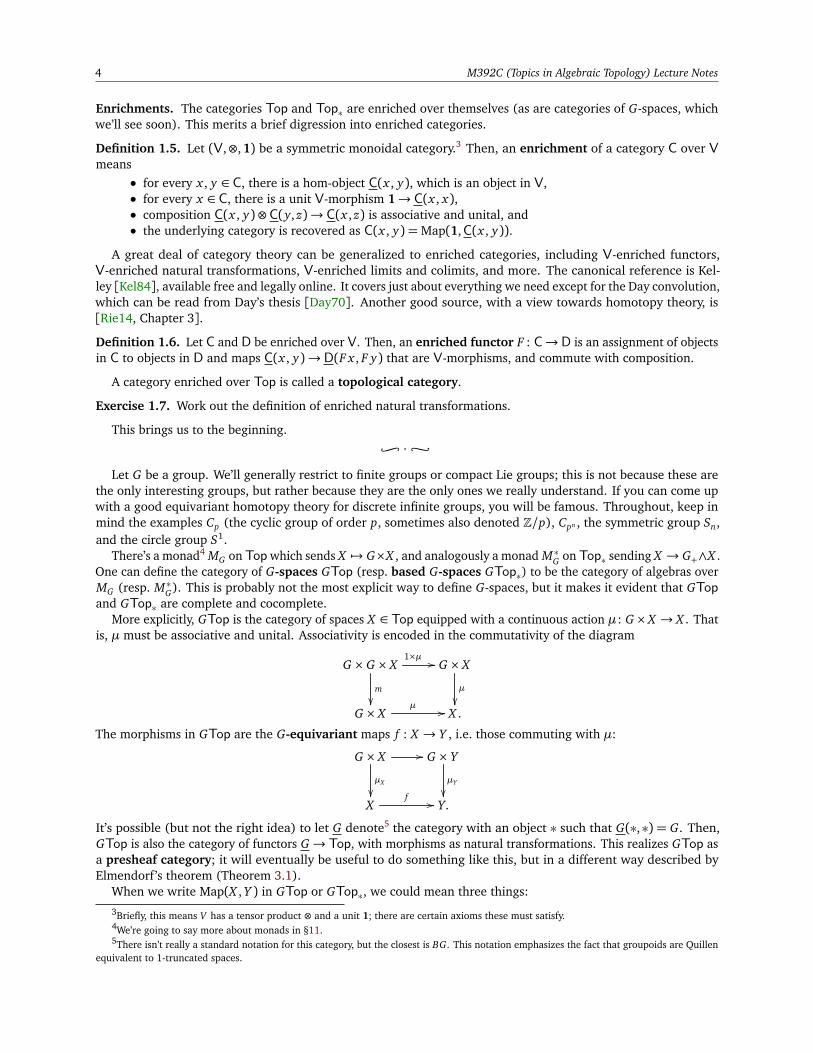
More explicitly, GTop is the category of spaces X ∈ Top equipped with a continuous action µ: G× X → X . Thatis, µ must be associative and unital. Associativity is encoded in the commutativity of the diagram
G × G × X1×µ //
m
G × X
µ
G × X
µ // X .
The morphisms in GTop are the G-equivariant maps f : X → Y , i.e. those commuting with µ:
G × X //
µX
G × Y
µY
X
f // Y.
It’s possible (but not the right idea) to let G denote5 the category with an object ∗ such that G(∗,∗) = G. Then,GTop is also the category of functors G→ Top, with morphisms as natural transformations. This realizes GTop asa presheaf category; it will eventually be useful to do something like this, but in a different way described byElmendorf’s theorem (Theorem 3.1).
When we write Map(X , Y ) in GTop or GTop∗, we could mean three things:
3Briefly, this means V has a tensor product ⊗ and a unit 1; there are certain axioms these must satisfy.4We’re going to say more about monads in §11.5There isn’t really a standard notation for this category, but the closest is BG. This notation emphasizes the fact that groupoids are Quillen
equivalent to 1-truncated spaces.
1 G-spaces: 1/17/17 5
(1) The set of G-equivariant maps X → Y .(2) The space of G-equivariant maps X → Y in the subspace topology of all maps from X → Y . As this
suggests, GTop admits an enrichment over Top (resp. GTop∗ admits an enrichment over Top∗).(3) The G-space of all maps X → Y , where G acts by conjugation: f 7→ g−1 f (g·). This realizes GTop as
enriched over itself, and similarly for GTop∗.
Each of these is useful in its own way: for constructions it may be important to be self-enriched, or to only look atG-equivariant maps. We will let MapG(X , Y ) or Map(X , Y ) denote (2) or its underlying set (1), and G Map(X , Y )denote (3).6
It turns out you can recover MapG from Map: the equivariant maps are the fixed points under conjugation ofall maps. This is written Map(X , Y )G =MapG(X , Y ).
Throughout this class, “subgroup” will mean “closed subgroup” unless specified otherwise.
Definition 1.8. Let X be a G-set and H ⊆ G be a subgroup. Then, the H-fixed points of X is the space X H :=x ∈ X | hx = x for all h ∈ H. This is naturally a WH-space, where WH = NH/H (here NH is the normalizer of Hin G).7
Definition 1.9. The isotropy group of an x ∈ X is Gx := h ∈ G | hx = x.
Isotropy groups are useful in the following two ways.
(1) Often, it will be helpful to reduce questions from GTop to Top using (−)H .(2) It’s also useful to induct over isotropy types.
Now, we’ll see some examples of G-spaces.
Example 1.10. Let H be a subgroup of G; then, the orbit space G/H is a useful example, because it corepresentsthe fixed points by H. That is, X H ∼= G Map(G/H, X ). These spaces will play the role of points when we buildthings such as equivariant CW complexes. (
Example 1.11. Let H ⊂ G as usual and U : GTop→ HTop be the forgetful functor. Then, U has both left andright adjoints:
• The left adjoint sends X to the balanced product G ×H X := G × X/ ∼, where (gh, x) ∼ (g, hx) for allg ∈ G, h ∈ H, and x ∈ X . Despite the notation, this is not a pullback! (In the based case, the balancedproduct is G+ ∧H X .) G acts via the left action on G. This is called the induced G-action on G ×H X .
• The right adjoint is MapH(G, X ) (or MapH(G+, X ) in the based case), the space of H-equivariant mapsG → X , with G-action (g f )(g ′) = f (g ′g). This is called the coinduced G-action on MapH(G, X ).8
Sometimes this is also denoted FH(G, X ). (
Remark. Here is a categorical perspective on “change of group.” Quite generally, a group homomorphism Gf−→H
induces adjunctions
GTop
f! //
f∗//
⊥
⊥HTopf ∗oo .
These are given by f!(X ) := H ×G X and f∗(X ) :=MapG(H, X ) for a G-space X , where H is given the structure of aG-space by f . When H = ∗, an H-space is just a space, and f!(X ) = XG is the space of orbits while f∗(X ) = X G is thespace of fixed points. Observe that similar statements hold for categories of modules, given a ring homomorphism
Rf−→S.In fact, these are both cases of very general abstract nonsense. Let BG denote the category with one object ∗
with Hom(∗,∗) = G; as we have said above, we can (naïvely) write GTop as the functor category TopBG . A group
homomorphism Gf−→H induces a functor BG
F−→BH (it is not quite true that the two are equivalent—think about
6Later, when we discuss G-spectra, we will use F(X , Y ) to denote function spectrum of X and Y as a G-spectrum, or FG(X , Y ) when Gneeds to be explicit.
7If H Å G, then X H is also a G/H-space.8This actually is a group action, since if a, b, g ∈ G, then (a(b f ))(g) = (b f )(ga) = f (gab) = (ab( f ))(g).
6 M392C (Topics in Algebraic Topology) Lecture Notes
why this is). Now f ∗ : HTop→ GTop is just restriction along F :
BG
F
f ∗(Y ) // Top
BHY
<<
According to abstract nonsense, restriction along F has left and right adjoints, called left and right Kan extensionalong F , respectively:
BG
F
X //
⇓η
Top
BHf!(X )=LanF X
<< BG
F
X //
⇑ε
Top
BHf∗(X )=RanF X
<<
These diagrams do not commute, but there are natural transformations Xη=⇒ f ∗ f!(X ) and f ∗ f∗(X )
ε=⇒X . When
H is the trivial group, BH is the trivial category, and it is known that left/right Kan extensions of a functor X alonga functor to the trivial category pick out the colimit/limit of X . That is, still viewing a G-space X as a functorBG→ Top, we have XG = colim
BGX and X G = lim
BGX .
For an example-driven introduction to Kan extensions, we recommend [Rie16, Chapter 6]. Like much ofcategory theory, this is ultimately all trivial, but it may be highly non-trivial to understand why it is trivial. (
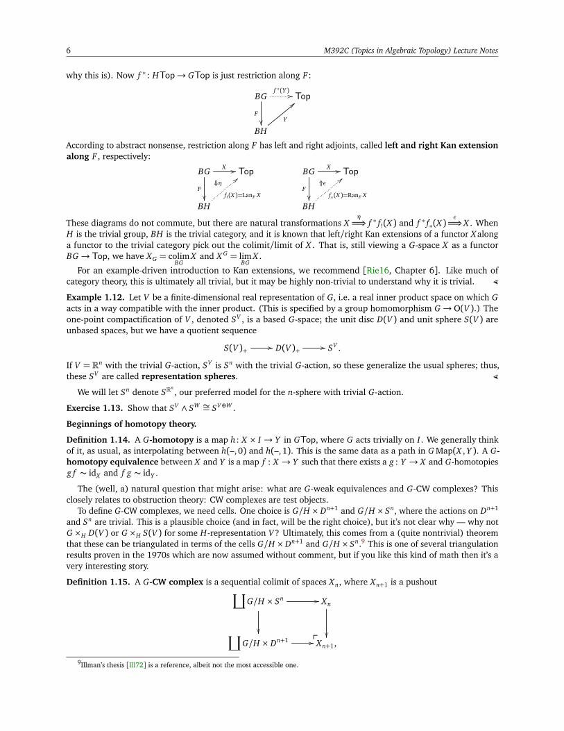
Example 1.12. Let V be a finite-dimensional real representation of G, i.e. a real inner product space on which Gacts in a way compatible with the inner product. (This is specified by a group homomorphism G→ O(V ).) Theone-point compactification of V , denoted SV , is a based G-space; the unit disc D(V ) and unit sphere S(V ) areunbased spaces, but we have a quotient sequence
S(V )+ // D(V )+ // SV .
If V = Rn with the trivial G-action, SV is Sn with the trivial G-action, so these generalize the usual spheres; thus,these SV are called representation spheres. (
We will let Sn denote SRn, our preferred model for the n-sphere with trivial G-action.
Exercise 1.13. Show that SV ∧ SW ∼= SV⊕W .
Beginnings of homotopy theory.
Definition 1.14. A G-homotopy is a map h: X × I → Y in GTop, where G acts trivially on I . We generally thinkof it, as usual, as interpolating between h(–, 0) and h(–,1). This is the same data as a path in G Map(X , Y ). A G-homotopy equivalence between X and Y is a map f : X → Y such that there exists a g : Y → X and G-homotopiesg f ∼ idX and f g ∼ idY .
The (well, a) natural question that might arise: what are G-weak equivalences and G-CW complexes? Thisclosely relates to obstruction theory: CW complexes are test objects.
To define G-CW complexes, we need cells. One choice is G/H × Dn+1 and G/H × Sn, where the actions on Dn+1
and Sn are trivial. This is a plausible choice (and in fact, will be the right choice), but it’s not clear why — why notG ×H D(V ) or G ×H S(V ) for some H-representation V? Ultimately, this comes from a (quite nontrivial) theoremthat these can be triangulated in terms of the cells G/H × Dn+1 and G/H ×Sn.9 This is one of several triangulationresults proven in the 1970s which are now assumed without comment, but if you like this kind of math then it’s avery interesting story.
Definition 1.15. A G-CW complex is a sequential colimit of spaces Xn, where Xn+1 is a pushout∐
G/H × Sn //
Xn
∐
G/H × Dn+1 // Xn+1,ð
9Illman’s thesis [Ill72] is a reference, albeit not the most accessible one.
2 G-spaces: 1/17/17 7
where H varies over all closed subgroups of G.
That is, it’s formed by attaching cells just as usual, though now we have more cells.This immediately tells you what the homotopy groups have to be: [G/H × Sn, X ], which by an adjunction game
is isomorphic to πn(X H). We let πHn (X ) := πn(X H). Thus, we can define weak equivalences.
Definition 1.16. A map f : X → Y of G-spaces is a weak equivalence if for all subgroups H ⊂ G, f∗ : πHn (X )→
πHn (Y ) is an isomorphism.
These homotopy groups have a more complicated algebraic structure: they’re indexed by the lattice of subgroupsof G and the integers. This is fine (you can do homological algebra), but some things get more complicated,including asking what the analogue of connectedness is! (We’ll broach this in Definition 2.8.)
One quick question: do we need all subgroups H? What if we only want finite-index ones? The answer, in avery precise sense, is that if you’re willing to use fewer subgroups, you get fewer cells G/H × Sn, and that’s fine,and you get a different kind of homotopy theory.
Finally, the Whitehead theorem (Corollary 2.12) is true for G-CW complexes. This follows for the same reasonas in May’s course: it follows word-for-word after proving the equivariant HELP (homotopy extension liftingproperty) lemma (Theorem 2.9) , which is true by the same argument as in the nonequivariant case.
We’ll next talk about presheaves on the orbit category, leading to Bredon cohomology.
Lecture 2.
Homotopy theory of G-spaces: 1/19/17
“It’s nice to write down, but oh so false.”
Last time, we saw the definition of a G-CW complex, but no examples were provided. Today, we’ll start with someexamples.
Recall that a G-CW complex is a sequential colimit X = colimn Xn, where Xn is formed by attaching cellsG/H ×Dn along maps G/H ×Sn−1→ Xn−1: just like the CW complexes we know and love, but with new cells G/Hindexed by the closed subgroups H ⊂ G. The idea is that you’re building up a space by attaching different spaceswith different isotropy groups (G/H has isotropy group H, just by construction).
Example 2.1 (Zero-dimensional complexes). The zero-dimensional complexes are G/H or disjoint unions qiG/Hi .This is an instance of the slogan that “orbits are points.” Keep in mind that if G is a compact Lie group, this mightnot be zero-dimensional in other, more familiar kinds of dimension. (
Example 2.2. Let S1 act on R2 by rotation along the origin. This also induces a Cn-action, as Cn ⊆ S1 as the nth
roots of unity. Let V denote this Cn-space.Let D(V ) denote the unit disc in V , and SV denote its one-point compactification, a representation sphere.
Then, D(V ) looks like wedges of pie, as the origin is fixed. On SV , the point at infinity is also fixed, so we obtain abeachball.
Now let’s consider V as an S1-space, and write down the CW structure on SV . There are two fixed points, andeach one is a 0-cell S1/S1 × ∗, but there is one 1-cell S1 × I attached to the endpoints (thought of as a meridianrotated around the sphere).
Now let’s consider the beachball for C2 on SV , where there are two hemispheres and C2 rotates by a half-turn.What’s the G-CW structure on this?
• There are two 0-cells C2/C2 × ∗, corresponding to the two fixed points, the north and south poles.• There is a single free 1-cell C2 × I , corresponding to the boundary of the hemispheres.• There is a single 2-cell C2 × D2. (
Last time, we discussed other prospective cells G ×H S(V ) and G ×H D(V ); these can be decomposed in termsof the actual cells we use. One point to observe about these cells is that G does not act on them by permutingnon-equivariant cells around, but rather in a more complicated way; there is virtue in the simplicity of the G-cellswe have chosen to work with.
Exercise 2.3. C2 also acts on S2 by the antipodal map, which has no fixed points. Write a C2-CW cell structure forthis C2-space.
8 M392C (Topics in Algebraic Topology) Lecture Notes
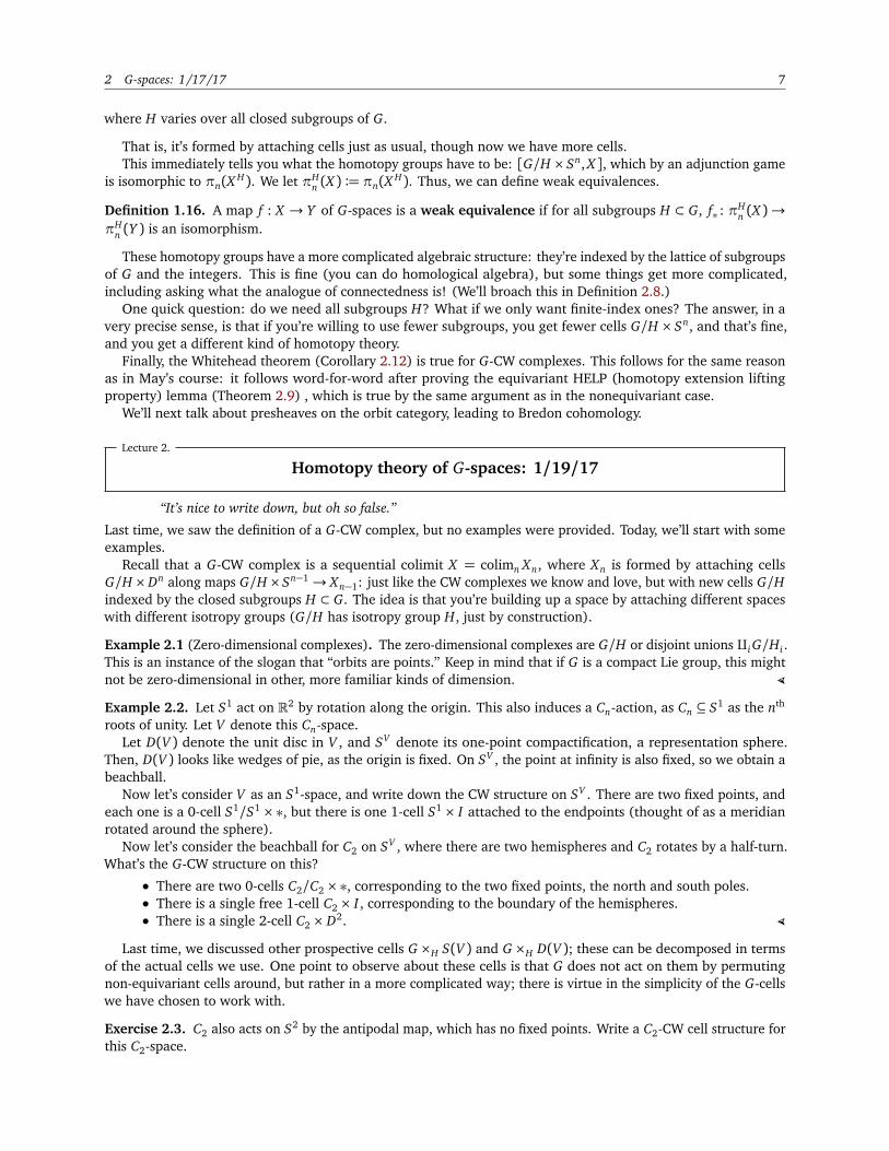
Example 2.4. The torus S1 × S1 has an S1-action given by z(z1, z2) = (zz1, z2). With this action, the torus can beviewed as an S1-CW complex with one 0-cell S1/e×∗ and one 1-cell S1 × [0, 1], with the attaching map sending 0and 1 to ∗. Note that the largest cell we used here was a 1-cell, whereas in the nonequivariant construction of thetorus, we are required to use a 2-cell. Check out Figure 1 for a picture. (
0-cellS1/e× ∗
1-cellS1/e× [0,1]
FIGURE 1. The S1-CW structure on the torus in Example 2.4. There is one 0-cell and one 1-cell.
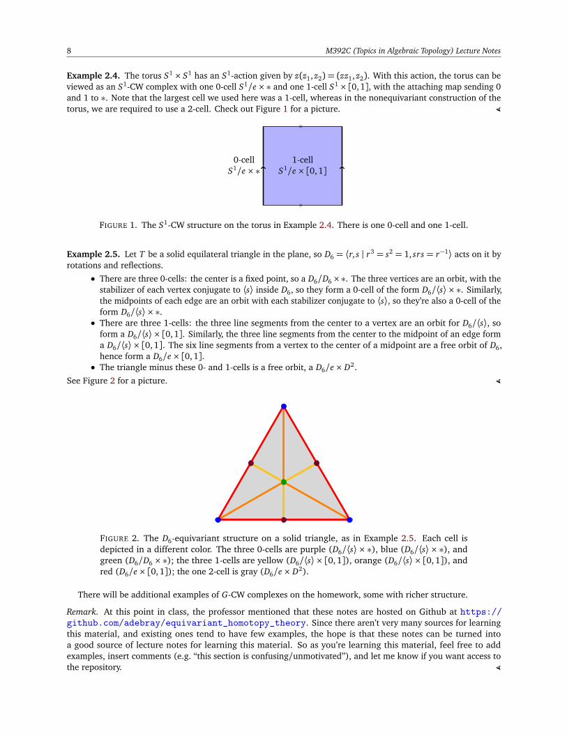
Example 2.5. Let T be a solid equilateral triangle in the plane, so D6 = ⟨r, s | r3 = s2 = 1, srs = r−1⟩ acts on it byrotations and reflections.
• There are three 0-cells: the center is a fixed point, so a D6/D6×∗. The three vertices are an orbit, with thestabilizer of each vertex conjugate to ⟨s⟩ inside D6, so they form a 0-cell of the form D6/⟨s⟩ × ∗. Similarly,the midpoints of each edge are an orbit with each stabilizer conjugate to ⟨s⟩, so they’re also a 0-cell of theform D6/⟨s⟩ × ∗.
• There are three 1-cells: the three line segments from the center to a vertex are an orbit for D6/⟨s⟩, soform a D6/⟨s⟩ × [0, 1]. Similarly, the three line segments from the center to the midpoint of an edge forma D6/⟨s⟩ × [0,1]. The six line segments from a vertex to the center of a midpoint are a free orbit of D6,hence form a D6/e× [0, 1].
• The triangle minus these 0- and 1-cells is a free orbit, a D6/e× D2.
See Figure 2 for a picture. (
FIGURE 2. The D6-equivariant structure on a solid triangle, as in Example 2.5. Each cell isdepicted in a different color. The three 0-cells are purple (D6/⟨s⟩ × ∗), blue (D6/⟨s⟩ × ∗), andgreen (D6/D6 × ∗); the three 1-cells are yellow (D6/⟨s⟩ × [0,1]), orange (D6/⟨s⟩ × [0,1]), andred (D6/e× [0, 1]); the one 2-cell is gray (D6/e× D2).
There will be additional examples of G-CW complexes on the homework, some with richer structure.
Remark. At this point in class, the professor mentioned that these notes are hosted on Github at https://github.com/adebray/equivariant_homotopy_theory. Since there aren’t very many sources for learningthis material, and existing ones tend to have few examples, the hope is that these notes can be turned intoa good source of lecture notes for learning this material. So as you’re learning this material, feel free to addexamples, insert comments (e.g. “this section is confusing/unmotivated”), and let me know if you want access tothe repository. (

2 Homotopy theory of G-spaces: 1/19/17 9
Remark.
(1) There is a technical issue of a G-CW structure on a product of G-CW complexes; namely, there are technicaldifficulties in cleanly putting a G-CW structure on G/H1×G/H2 involving triangulation. We won’t digressinto this: it’s straightforward for finite groups, but a theorem for compact Lie groups, and requiredrevisiting the foundations. Similarly, if H ⊂ G, we’d like the forgetful functor GTop → HTop to sendG-CW complexes to H-CW complexes. This is again possible, yet involves technicalities.
(2) A nicer fact is that computing the fixed points of a G-CW complex is straightforward. Recall that (–)H is aright adjoint, which can be seen by realizing it as the limit of the diagram
•
H
// Top.
Thus, we don’t expect it to commute with colimits in general. However, it does commute with manyimportant ones, as in the following proposition. (
Proposition 2.6. The fixed point functor (–)H commutes with
(1) pushouts where one leg is a closed inclusion, and(2) sequential colimits along closed inclusions.
This is great, because it means we can commute (–)H through the construction of a G-CW complex! In particular,on each cell,
(G/K × Dn)H ∼= (G/K)H × Dn,
so we need to understand (G/K)H ∼=MapG(G/H, G/K). We will return to this important point.
Two approaches to the Whitehead theorem. We’ll now discuss some homotopy theory of G-spaces and theWhitehead theorem. The first will be a hands-on proof using the HELP lemma. This is an elegant approach tounstable homotopy theory due to Peter May in which one lemma gives quick proofs of several theorems. In theequivariant case, it allows a quick reduction to the non-equivariant case; it will be useful to see a proof of thisnature. Ultimately, we will take a different approach involving model categories, and this will be the secondperspective.
Definition 2.7. Let X , Y ∈ Top and f : X → Y be continuous. Then, f is n-connected if πq( f ): πq(X )→ πq(Y )is an isomorphism when q < n and surjective when q = n.
We wish to generalize this to the equivariant case.
Definition 2.8. Let θ : conjugacy classes of subgroups of G → x ∈ Z | x ≥ −1.• A map f : X → Y of G-spaces is θ -connected if for all H ⊂ G, f H is θ (H)-connected.• A G-CW complex is θ -dimensional if all cells of orbit type G/H have (nonequivariant) dimension at mostθ (H).
Theorem 2.9 (Equivariant HELP lemma). Let A, X , Y , and Z be G-CW complexes such that A⊆ X is θ -dimensionaland let e : Y → Z be a θ -connected G-map. Given g : A→ Y , h: A× I → Z, and f : X → Z such that eg = hi0 andf i = hi1, there exist maps g : X → Y and h: X × I → Z that make the following diagram commute:
A
i0 // A× I
h
||
Ai1oo
g
Z Yeoo
X
f??
i0// X × I
h
bb
Xi1
oog
__
This is a massive elaboration of the idea of a Hurewicz cofibration. The best way to understand this is to proveit (though it’s not an easy proof).
10 M392C (Topics in Algebraic Topology) Lecture Notes
In the non-equivariant case, one reduces to working one cell at a time, inductively extending over the cells of Xnot in A.10 In this case, look at Sn−1 ⊆ Dn. Now you just do it: at this point, there’s no way to avoid writing downexplicit homotopies.
Exercise 2.10. Think about this argument, and then read the proof in [May99].
The equivariant case is very similar: in the same way, one can reduce to inductively attaching a single cell inthe case where X is a finite CW complex. This comes via a map G/H × Sn−1→ G/H × Dn, but the only interestingcontent is in the nonequivariant part, so we can reduce again to Sn−1 → Dn with trivial G-action! This allowsus to finish the proof in the same way. It also says that the homotopy theory of G-spaces is lifted from ordinaryhomotopy theory, in a sense that model categories will allow us to make precise.
The first consequence of Theorem 2.9 is:
Theorem 2.11. Let e : Y → Z be a θ -connected map and e∗ : [X , Y ]→ [X , Z] be the map induced by composition.• If X has dimension less than θ , e∗ is a bijection.11
• If X has dimension θ , e∗ is a surjection.
The proof is an exercise; filling in the details is a great way to get your hands on what the HELP lemma isactually doing. Hint: consider the pairs ∅→ X and X × S0→ X × I , and apply the HELP lemma.
Corollary 2.12 (Equivariant Whitehead theorem). Let e : Y → Z be a weak equivalence of G-CW complexes. Then,e is a G-homotopy equivalence.
Proof. This is also a standard argument: using Theorem 2.11, e∗ is a bijection, so we can pull back idZ ∈ [Z , Z] toan inverse (e∗)−1(idZ) ∈ [Z , Y ], which is a homotopy inverse to e.
One can continue and prove the cellular approximation theorem in this way, and so forth. We won’t do this,because we’ll approach it from a model-categorical perspective.
One thing that’s useful, not so much for this class as for enriching your life, is to learn how to approach thisfrom the perspective of abstract homotopy theory, learning about disc complexes and so forth. You can provetheorems such as the HELP lemma and its consequences in a general setting, and then specialize them to the casesyou need. This is a great way to “just do it” without needing model categories.
Anyways, we’ll now define a model structure on GTop and GTop∗. If you don’t know what a model category is,now is a good time to review.
Proposition 2.13. There is a model structure on GTop (and on GTop∗) defined by the following data.Cofibrations: The maps f : X → Y such that for all H ⊂ G, f H : X H → Y H is a cofibration.Weak equivalences: The maps f : X → Y such that for all H ⊂ G, f H : X H → Y H is a weak equivalence.
So we once again parametrize everything over subgroups of G and use fixed points. This is a cofibrantlygenerated model category; the cofibrations are specified by generators of acyclic cofibrations in a similar mannerto Top. That is, in Top, one can choose generators I = Sn−1→ Dn and J = Dn→ Dn × I; in GTop, we insteadtake IG = G/H × I and JG = G/H × J.
These are cells that we used to define G-CW complexes, and this is no coincidence: it’s a general fact aboutcofibrantly generated model categories that follows from the small object argument12 that cofibrant objects areretracts of “cell complexes” built from the things in I , and cofibrations are retracts of cellular inclusions of cellcomplexes. In this sense, CW complexes are inevitable.
The Whitehead theorem (Corollary 2.12) now falls out of the general theory of model categories.
Theorem 2.14 (Whitehead theorem for model categories). Let f : X → Y be a weak equivalence of cofibrant-fibrantobjects in a model category. Then, f is a homotopy equivalence.
In Top and GTop, all objects are fibrant, so this is particularly applicable.10This requires reducing to the case where X is a finite CW complex, but taking a sequential colimit recovers the theorem for all CW
complexes X .11We say that X has dimension less than θ if for all closed subgroups H ⊂ G, all cells of orbit type G/H have (nonequivariant) dimension
at most n for some n≤ θ (H).12The small object argument is a beautiful piece of basic mathematics that everybody should know. If you don’t know it, your homework is
to read enough about model categories to get to that point. In general, there may be large objects and transfinite induction, but for the case wecare about large cardinals won’t arise.
3 Homotopy theory of G-spaces: 1/19/17 11
The orbit category. We’ll begin talking about the orbit category in the rest of today’s lecture, and discuss the barconstruction next class.
Definition 2.15. The orbit category OG is the full subcategory of GTop on the objects G/H.
That is, its objects are the spaces G/H, where H ⊂ G is closed, and its morphisms are MapG(G/H, G/K) ∼=(G/K)H . These maps are the same thing as subconjugacy relations, i.e. those of the form
(2.16) gH g−1 ⊆ K ,
since for all h ∈ H, h(gK) = gK if and only if K = g−1hgK if and only if gH g−1 ⊆ K. A G-map f : G/H → G/Kis completely specified by what it does to the identity coset f (eH) = gK, and this g implies the subconjugacyrelation (2.16), since, as above, h(gK) = gK for all h ∈ H.
There’s another description of the orbit category.
Proposition 2.17. Let G be a finite group. Then, the orbit category OG is equivalent to the category of finite transitiveG-sets and G-maps.
The observation that ignites the proof is that if x ∈ X has isotropy group H, then its orbit space is isomorphic toG/H.
Definition 2.18. Given a G-space X , we obtain a presheaf on the orbit category, namely a functor X (–) : O opG → Top,
by sending G/H → X H . This assignment itself is a functor ψ: GTop→ Fun(O opG ,Top).
Proposition 2.19. Fun(O opG ,Top) has a projective model structure where the weak equivalences and fibrations are
taken pointwise.
The point is the following result, a revisionist interpretation of Elmendorf’s theorem. Elmendorf’s originalproof [Elm83] showed these two categories have the same homotopy theory, but his proof was more explicit anddid not use model categories.
Theorem 2.20 (Elmendorf [Elm83, Ste16]). ψ is the right adjoint in a Quillen equivalence; the left adjoint θ isevaluation at G/e.
The point is, these two model categories have the same homotopy theory.
Exercise 2.21. Check that evaluation at G/e is a left adjoint to ψ.
Lecture 3.
Elmendorf’s theorem: 1/24/17
“What’s bad about this proof?”“It appeals to machinery we didn’t develop in this class?”“No, that’s perfectly fine.”
We’ll start by reviewing the connection between the orbit category and G-sets.Let X be a finite G-set. Then, X is the coproduct (disjoint union) of a bunch of orbits:
X ∼=∐
i
G/Hi .
The way you see this is that for any x ∈ X , its orbit is isomorphic to G/Gx . This is yet another manifestation of theslogan that “orbits are points.” But it also implies that, rather than just presheaves on OG , one could work withcertain presheaves on the category of finite G-sets, and this perspective will turn out to be useful. By “certain” wemean a compatibility with orbits.
Last time, we talked about Elmendorf’s theorem in the form of Theorem 2.20. It’s also possible to state it in amore general form.
Theorem 3.1 (Elmendorf). The functor GTop → Fun(O opG ,Top) determined by X 7→
G/H 7→ X H
induces anequivalence of (∞, 1)-categories, where the weak equivalences on the left and right are specified by a family F .
Without delving into (∞, 1)-categories, this means• the homotopy categories are equivalent, and• homotopy limits and colimits behave identically.
12 M392C (Topics in Algebraic Topology) Lecture Notes
In other words, from the perspective of abstract homotopy theory, these are the same.
Definition 3.2. By a family of subgroupsF of G, we mean a collection of subgroups of G closed under conjugationand taking subgroups.
Examples include the set of all subgroups, the set of just the identity, and the set of finite subgroups. The latteris useful for some S1-equivariant spaces, where one tends to lose control of the S1-fixed points, but the finitesubgroups behave better.
Definition 3.3. Let F be a specified family of subgroups of G.
• In GTop, the weak equivalences specified by F are the maps f : X → Y such that f H : X H → Y H is a weakequivalence for all H ∈ F .
• For Fun(O opG ,Top), a weak equivalence specified by F is a pointwise weak equivalence at G/H for all
H ∈ F .
We’ll give two proofs of Theorem 3.1. The first will be model-categorical.
Recall13 if F : C//
⊥ D :Goo is a Quillen adjunction, then the left and right derived functors (LF,RG) is anadjunction on the homotopy categories (HoC,HoD). If K denotes fibrant replacement in D and Q denotescofibrant replacement in C, then the derived functors are LF = FQ and RG = GK .14
Definition 3.4. That (F, G) is a Quillen equivalence means that for any cofibrant X ∈ C and fibrant Y ∈ D, thenFX → Y is a weak equivalence iff its adjoint X → GY is.
This is equivalent to asking that (LF,RG) are equivalences of categories.This is a kind of curious way to look at an equivalence of categories. One says that G : D→ C creates the weak
equivalences of D if for every morphism f of D, f is a weak equivalence iff G f is.
Lemma 3.5. If G creates the weak equivalences of D and for all cofibrant X the unit map X → GFX is a weakequivalence, then (F, G) is a Quillen equivalence.
This is a useful tool for extending model categories along free-forgetful adjunctions; for example, if you have amodel category and want to understand abelian group or ring objects in this category, often their weak equivalencesare detected by the forgetful functor.
Proof sketch of Theorem 3.1. We want to apply Lemma 3.5 to the adjunction
Fun(O opG ,Top)
θ //⊥ GTopψoo ,
where θ : X 7→ X (G/e) is evaluation at G/e and ψ: Y 7→ Y H. The first condition, that ψ detects the weakequivalences, is straightforward, so we need to check that X 7→ X (G/e)H is a weak equivalence for all cofibrantX .
Cellular objects model the generating cofibrations, so cofibrant objects are retracts of cellular objects. Sinceweak equivalences are preserved under retracts, then we can check on cellular objects. Here it’s easier, since (–)H
commutes with the relevant colimits and is suitably cellular.
The missing steps in this proofs can be filled in by explicitly identifying the cofibrant objects in Fun(O opG ,Top).
These are free diagrams on the orbit category; not hard to write down, but messy enough to avoid on the chalkboard.
Remark. Elmendorf’s original proof of his theorem was in the 1980s and did not use model categories, even thoughQuillen had already introduced them at the time. Until the mid-1990s (30 years after [CITE ME: “Homotopicalalgebra”]), many homotopy theorists avoided them, thinking of them as formal gobbledygook. However, about thetime EKMM introduced a symmetric monoidal category of spectra, people began realizing they were unavoidable.
(
13If this is not review to you, then exercise: learn this material!14This does require cofibrant and fibrant replacement to be functorial, which is not true in every model category, but will be true for pretty
much everything we study.
3 Elmendorf ’s theorem: 1/24/17 13
You might not like the given proof of Elmendorf’s theorem because it’s extremely inexplicit: cofibrant replacementis an infinite process, and many of the steps involved are quite abstract. The next proof will be more explicit,building a (homotopical) right adjoint to ψ.
This proof will go through the bar construction, a categorical tool that’s extremely useful. References forit include May’s “Geometry of iterated loop spaces” [May72], Riehl’s monograph [Rie14], and Vogt’s “Tensorproducts of functors.”
Second proof of Theorem 3.1. Let M : OG → Top realize orbits as spaces: G/H is sent to the topological space G/H,and an equivariant map f is forgotten to a continuous map f .
Given an X ∈ Fun(O opG ,Top), let
Φ(X ) := |B•(X ,OG , M)|denote the geometric realization of the simplicial bar construction. Let’s be a little more explicit about this.B•(X ,OG , M) is a simplicial space that sends
[n] 7−→∐
G/Hn−1→···→G/H0
X (G/H0)×M(G/Hn−1).
As usual, the face maps are defined by composition, and the degeneracies by inserting the identity map. Since Gacts on M(–) simplicially (i.e., in a way compatible with the face and degeneracy maps), then |B•(X ,OG , M)| is aG-space (passing through the coend formula for the geometric realization).
If H ⊆ G, we want to understand Φ(X )H . Because the G-action passed through geometric realization,
Φ(X )H ∼= |B•(X ,OG , M H)| ∼= |B•(X ,OG , MapOG(G/H, –))|.
Let X (G/H) denote the constant simplicial space [n] 7→ X (G/H). Then, by general theory of the bar constructionfor any corepresented functor, there’s a simplicial map
(3.6) B•(X ,OG ,MapOG(G/H, –)) −→ X (G/H)
defined by composing and applying X , and this is a simplicial homotopy equivalence (you can write down aretraction).15 Thus, Φ(X )H ∼= X (G/H). In other words, Φ is a homotopy inverse, since taking H-fixed points ofΦ(X ) gives back what you started with.
Φ(X ) is still an infinite-dimensional object, but it’s much more explicit, and you can work with it.
Applications of this perspective. We’ll be able to use Elmendorf’s theorem to make some constructions thatwould be hard to imagine without the orbit category.
Definition 3.7. Let F be a family of subgroups of G. Then, the classifying space for F is specified by theuniversal property that if Z has F -isotropy, then [Z , EF ] has a unique element. An explicit construction is to leteEF denote the presheaf on the orbit category where
eEF (G/H) :=
¨
∗, H ∈ F∅, H 6∈ F ,
and let EF := Φ(eEF ).
If you unwind the definition, this is the bar construction applied to G in the category of G-spaces with weakequivalences given by F , meaning it deserves to be called a classifying space.
Another useful notion is the G-connected components.
Definition 3.8. Let X be a G-space and x ∈ X G . Let Yx be the presheaf on the orbit category sending H to theconnected component containing x ∈ X H . Then, the G-connected component of x is Φ(Yx).
The third useful application is defining Eilenberg-Mac Lane spaces. This will lead us to cohomology (and thento Smith theory and other things). These will be constructed by working pointwise, then applying Φ.
Definition 3.9. Let G be a finite group, A coefficient system is a presheaf X ∈ Fun(O opG ,Ab).16
15This is called an extra degeneracy argument in the literature. There’s an observation probably due to John Moore which approximatelysays that if you have a simplicial object with an extra degeneracy condition playing well with the preexisting ones, then it must be contractible;this argument is applied to the fiber of (3.6).
16For G a compact Lie group, the definition is almost the same, but we need to use Fun(hO opG ,Ab), taking presheaves on the homotopy
category. For finite groups these definitions coincide.
14 M392C (Topics in Algebraic Topology) Lecture Notes
Elmendorf’s theorem says that for any coefficient system, we have an Eilenberg-Mac Lane G-space. You could sayhere that (Bredon) cohomology is completely determined: cohomology is the things represented by Eilenberg-MacLane spaces. But it will be good to see it explicitly. Bredon cohomology is explicit, but there are serious drawbacks:it has poor formal properties, and you need a lot of geometric insight to compute things. We’ll later see that thisabelian category (meaning we can do homological algebra) is the wrong one; we’ll later see this is a Z-gradedcohomology theory (or rather graded on subgroups of Z); this will be the wrong answer, especially if you wantPoincaré duality, and the right answer uses a grading by the representation ring. But we’ll get there.
Remark. Another application of Elmendorf’s theorem, which we will not discuss in detail (unless we get to the slicefiltration), is Postnikov towers. They’re constructed in the same way, by either using the small object argument orkilling homotopy groups. (
Coefficient systems have an important role in Bredon cohomology, which is calculated with coefficients ina coefficient system, and whose construction makes use of a chain complex of coefficient systems. In this way,coefficient systems play the part in Bredon cohomology that abelian groups do in CW cohomology. Indeed,coefficient systems form an abelian category; it may be helpful to think of it as the category of “right OG-modules,”even if that isn’t literally true.
Here are some examples of coefficient systems (which are often denoted with underlines).
Example 3.10.
(1) Z will denote the constant coefficient system with coefficients in Z, i.e. the functor which sends allobjects to Z and all morphisms to idZ. You can replace Z with your favorite abelian group.
(2) For a G-space X , the coefficient system πn(X ) (n ≥ 2) sends G/H 7→ πnX H. This is an example ofa general formula: given a functor Top → Ab, we can compose to obtain a map Fun(O op
G ,Top) →Fun(O op
G ,Ab).(3) In the same way, Hn(X ) sends G/H 7→ Hn(X H ;Z). (
We will now define Bredon cohomology, due to Bredon [Bre67], which is the analogue of CW cohomology forG-CW complexes.
Definition 3.11. We first define a chain complex of coefficient systems C•(X ), which is the analogue of the CWchain complex. It sends an orbit G/H to the CW chains of X H .17
Let X be a G-CW complex and Xn denote its n-skeleton. Let
Cn(X ) := Hn(Xn, Xn−1;Z),
i.e. the coefficient system sending G/H 7→ Hn((X H)n, (X H)n−1;Z) = CCWn (X
H). The differential at G/H is theCW chain complex differential for X H , i.e. the connecting morphism in the long exact sequence of the triple((X H)n, (X H)n−1, (X H)n−2). One should check that this commutes with the bonding maps for Cn(X ), but it does, sothis works.
The Bredon cohomology with coefficients in a coefficient system M is
HnG(X ; M) := Hn
HomFun(O opG ,Ab)(C•(X ), M)
.
That is, we take the chains on X and compute the maps into M ; since Fun(O opG ,Ab) is an abelian category, this
is a cochain complex of abelian groups, and we can take its homology to obtain a sequence of abelian groups.We’ll continue to discuss Bredon cohomology next lecture, and introduce an axiomatic viewpoint. This is basic
and fundamental, but not too relevant to the rest of the class. It’s also good to calculate; there are surprisingly fewexamples out in the world.
Lecture 4.
Bredon cohomology: 1/26/17
“Smith’s theorem was proven by Smith, hence the name.”
17This requires knowing how to obtain a CW structure on X H given a G-CW structure on X . If G is finite, this is easy to see; for generalcompact Lie groups, though, this requires a triangulation argument. One wants the resulting coefficient system to be independent of the choiceof triangulation, but as in the nonequivariant case, this is proven via an axiomatic characterization of cohomology.
4 Bredon cohomology: 1/26/17 15
Today we’ll continue Bredon cohomology, and state a version of the Eilenberg-Steenrod axioms that characterize it.Then, we’ll turn to the circle of ideas around Smith theory, including the Sullivan conjecture (which we won’tprove, because it’s hard). Smith theory is about when one can recover H∗(X G) from algebraic information derivedfrom the G-action on X .
Let’s recall the definition of Bredon cohomology from last time: if X is a G-CW complex, let C∗(X ) denote thechain complex of coefficient systems (i.e. functors O op
G → Ab)
Cn(X )(G/H) := Hn((XH)n, (X H)n−1;Z).
The differential ∂ : Cn(X )→ Cn−1(X ) is the same as in CW cohomology, the connecting morphism in the long exactsequence for the triple (Xn, Xn−1, Xn−2); that ∂ 2 = 0 is something you have to check, though it’s not very difficult.
Using this chain complex, we define Bredon homology and cohomology.
• The Bredon cohomology with coefficients in a coefficient system M is
HnG(X ; M) := Hn(HomFun(O op
G ,Ab)(C∗(X ), M)).
We defined this last time.• For homology to be a covariant functor, we need the coefficient system M to be a functor OG → Ab rather
than O opG → Ab (e.g. H∗(X ) for a G-space X , which sends G/H 7→ Hn(X H)).18 With M such a coefficient
system, the Bredon homology with coefficients in M is
HGn (X ; M) := Hn(Cn(X )⊗OG
M).
By this tensor product, we mean a coend:
Cn(X )⊗OGM =
∫ G/H∈OG
Cn(X )(G/H)⊗M(G/H)
=⊕
G/H
Cn(X )(G/H)⊗M(G/H) /∼,
where if f ∈MapOG(G/H, G/K), ( f ∗ y, z)∼ (y, f∗z).
19
The whole philosophy of Bredon (co)homology is to understand equivariant cohomology and homology throughthe fixed-point sets and the lattice of subgroups of G.
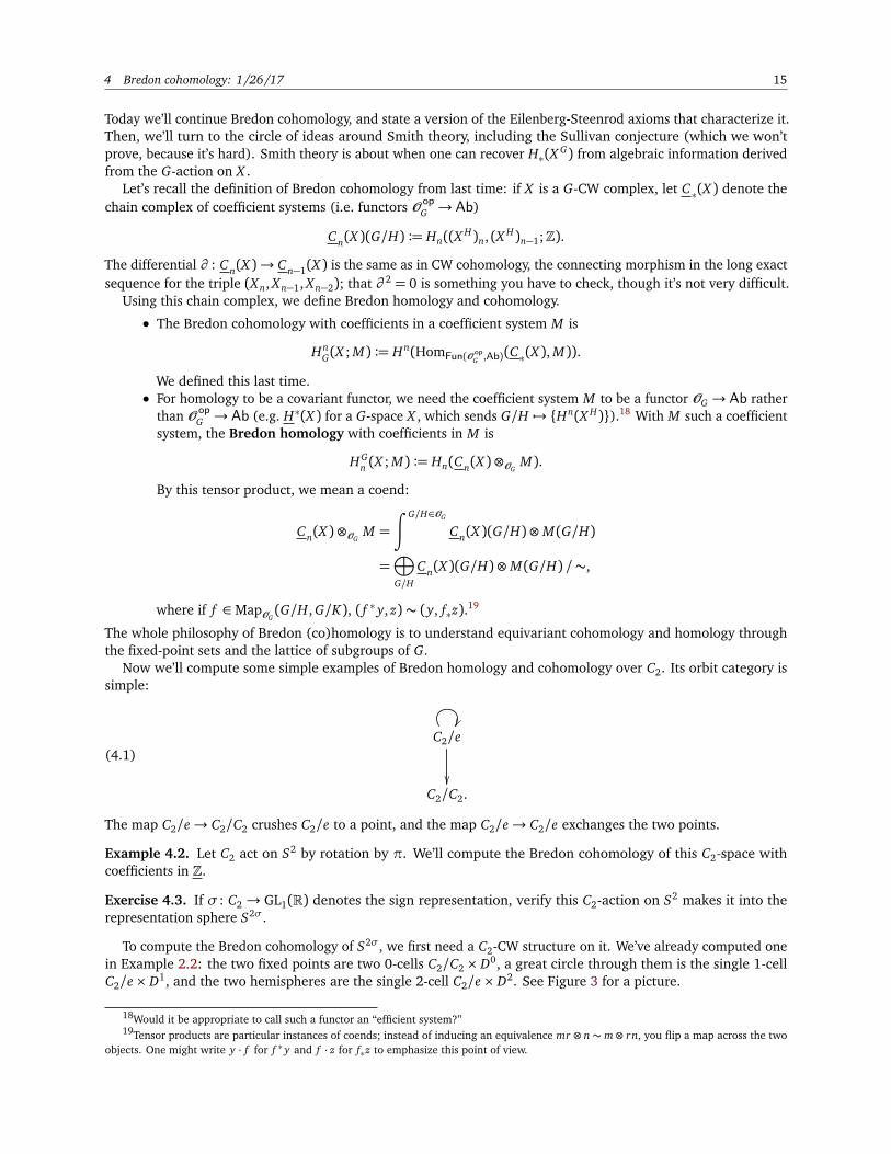
Now we’ll compute some simple examples of Bredon homology and cohomology over C2. Its orbit category issimple:
(4.1)C2/e
C2/C2.
The map C2/e→ C2/C2 crushes C2/e to a point, and the map C2/e→ C2/e exchanges the two points.
Example 4.2. Let C2 act on S2 by rotation by π. We’ll compute the Bredon cohomology of this C2-space withcoefficients in Z.
Exercise 4.3. If σ : C2 → GL1(R) denotes the sign representation, verify this C2-action on S2 makes it into therepresentation sphere S2σ.
To compute the Bredon cohomology of S2σ, we first need a C2-CW structure on it. We’ve already computed onein Example 2.2: the two fixed points are two 0-cells C2/C2 × D0, a great circle through them is the single 1-cellC2/e× D1, and the two hemispheres are the single 2-cell C2/e× D2. See Figure 3 for a picture.
18Would it be appropriate to call such a functor an “efficient system?”19Tensor products are particular instances of coends; instead of inducing an equivalence mr ⊗ n∼ m⊗ rn, you flip a map across the two
objects. One might write y · f for f ∗ y and f · z for f∗z to emphasize this point of view.

16 M392C (Topics in Algebraic Topology) Lecture Notes
FIGURE 3. A C2-CW structure on S2σ, the 2-sphere with a C2-action by rotation through 180.The two green dots are the two 0-cells C2/C2 × D0; the red circle is the single 1-cell C2/e× D1,and the gray hemispheres are the single 2-cell C2/e× D2.
Next we compute C∗(S2σ). A coefficient system is determined by a map M1→ M2 and an involution on M2. In
our case, C k(X )(C2/e) = Z⊕Z for k = 0, 1, 2, and the involution flips the two factors. Therefore we obtain a chaincomplex of coefficient systems which is
0 // Z⊕Zf1 // Z⊕Z
f2 // Z⊕Z // 0
at C2/e and
(4.4) 0 // 0 // 0 // Z⊕Z // 0
at C2/C2. Next we need to determine the differentials. By definition, these are determined by the cellular boundarymaps, i.e. the attaching maps. Let (x , y) denote the standard basis of Z⊕Z.
• f1 sends (x , y) 7→ (x + y, x + y).• f2 sends (x , y) 7→ (x − y, y − x),
Next, we compute the Hom from this coefficient system to the constant coefficient system Z. These groupsare evidently determined by what happens at the C2/e spot. For the first two terms, we are looking at mapsZ⊕Z→ Z that are equivariant (where g ∈ C2 acts by transposition on the left and trivially on the right). Such amap is determined by where it sends (1, 0), and so these two terms are isomorphic to Z. The last term is simply allhomomorphisms Z⊕Z→ Z⊕Z, which is isomorphic to Z⊕Z. Therefore, we have the cochain complex
0 // Z⊕Z // Z // Z // 0.
Computing the differentials, we find that the first map is (a, b) 7→ a+ b and the second map is 0.Taking the cohomology of this complex then produces
Hn(S2σ;Z) =
¨
Z, n= 0,2
0, otherwise.
Now, we’ll compute the Bredon homology of S2σ, again with coefficients in the constant functor valued in Z. Firstwe need to compute the tensor product C•(X )⊗OC2
Z:
Z2 Z2/⟨[1,−1]⟩
1−1
oo Z2/⟨[1,−1]⟩.0oo
Hence the Bredon homology of S2σ is
HC2
k (S2σ;Z) =
Z2, k = 0
Z, k = 2
0, otherwise.
TODO: shouldn’t it be Z, 0, Z? (
Remark. We’re used to reading off properties of a space from its cohomology, and this is still true here, if harder.For example, H0 tells us the number of connected components of S2/C2. (

4 Bredon cohomology: 1/26/17 17
Exercise 4.5. Generalize Example 4.2 to Snσ, the n-sphere with a C2-action given by a half-turn.
Example 4.6. Let C2 act on S2 by the antipodal action. We get a C2-CW structure of TODO. We’ll again computethe Bredon cohomology of S2 with coefficients in Z.
The chain complex C•(X ) is
Z2
0 11 0
Z2
1 −1−1 1
oo
0 11 0
Z2
1 11 1
oo
0 11 0
0
OO
0
OO
oo 0.
OO
oo
Now we need to take Hom(–,Z). In each degree we get a one-dimensional space of maps generated by (1, 1). Thedifferential ∂ : C0→ C1 sends
(1, 1) 7−→ (1,1)
1 −1−1 1
=
00
,
and the differential ∂ : C1→ C2 sends
(1,1) 7−→ (1, 1)
1 11 1
=
22
.
Hence the cochain complex is
Z 0 // Z 2 // Z,so the Bredon cohomology is
HkC2(S2;Z) =
Z, k = 0
Z/2, k = 1
0, otherwise,
which is exactly the cohomology of RP2 = S2/C2. (
This is no coincidence: if G acts freely on X , then the Bredon cohomology and homology is that of the quotient.
Exercise 4.7. Let G act freely on a CW complex X , let M : O opG → Ab, and let N : OG → Ab. Show that
H∗G(X ; M)∼= H∗(X/G; M(G/e)) and HG∗ (X ; N)∼= H∗(X/G; N(G/e)).
Corollary 4.8. If G acts on X trivially, H∗G(X ; M)∼= H∗(X ; M(e)), and similarly for homology.
Example 4.9. Let’s generalize to Cn. Let Cn act on S2 by rotation through an angle 2π/n. If V denotes the2-dimensional Cn-representation generated by a rotation through 2π/n, then this Cn-space is the representationsphere SV .
The C2-CW structure on S2σ from Example 4.2 generalizes to the “beachball” Cn-CW structure on SV :
• There are two 0-cells Cn/Cn × D0, which are the fixed points.• There is a single 1-cell Cn/e× D1, which is n equally spaced meridians.• There is a single 2-cell Cn/e× D2, which fills in the rest of the sphere.
We’ll first compute Bredon cohomology with respect to the trivial family F0 of subgroups of Cn, i.e. just Cnand e. The orbit category looks similar to the one for C2 (4.1), but there are more automorphisms of Cn/e:MapCn(Cn/e, Cn/e)∼= (Cn/e)e, so there are n of them. Namely, for 0≤ i < n, let ϕi send x 7→ x + i mod n; theseare equivariant, so we’ve found them all. Thus the orbit category for the trivial family of subgroups of Cn is
Cn/e
ϕ0,...,ϕn−1
Cn/Cn.
Since ϕ1 generates AutOCn(Cn/Cn), we’ll keep track of it and leave the rest of the ϕi implicit.

18 M392C (Topics in Algebraic Topology) Lecture Notes
First, we calculate C•(SV ). At Cn/e, this is just the CW chains for S2, but with the nonequivariant CW structure
induced by forgetting the Cn-action on SV . That is, there are two 0-cells, n 1-cells, and n 2-cells:
Z2 Znoo Zn.oo
At Cn/Cn, this is the CW chains for the fixed points, which are an S0:
Z2 0oo 0oo
just as in (4.4).Next we should figure out the bonding maps. Since the fixed points are the 0-skeleton, the maps in C0(S
V ) areall the identity. In degrees 1 and 2, ϕ∗1 : Zn→ Zn is the shift matrix sending the standard basis vector ei 7→ ei+1 mod n.
Next the differentials. Let e1 denote the north pole, e2 denote the south pole, f1, . . . , fn denote the 1-cells andg1, . . . , gn denote the 2-cells. Orient the 1-cells as pointing north and the 2-cells as counterclockwise if the northpole is at the top.
• For d : C1(SV )→ C0(S
V ), d( fi) = e1 − e2 and thus is the matrix
A :=
1 1 · · · 1−1 −1 · · · −1
.
• For d : C2(SV )→ C1(S
V ), d(gi) = fi+1 mod n − fi , so its matrix is
B :=
−1 11 −1
1.... . .
−1
.
Thus C•(X ) is
(4.10)Z2
id
ZnAoo
ϕ∗1
ZnBoo
ϕ∗1
Z2
id
OO
0oo
OO
0.oo
OO
Next we apply Hom(–,Z). The cochain complex is
Z2 d0// Z d1
// Z,
and the differentials are:
• d0 : Z2→ Z is the matrix
1 −1
.• d1 : Z→ Z is the zero map.
Hence
(4.11) HkG;F0(SV ) =
¨
Z, k = 0,2
0, otherwise.
It would also be good to compute the Bredon cohomology with respect to the complete family, but depending onn, this could get complicated. If n is prime, the complete and trivial families coincide, so we’re done. A slightlymore interesting example is n= p2, where p is prime. In this case the orbit category is
(4.12)
Cp2/e
Cp2tt
Cp2/Cp
Cp
Cp2/Cp2 .
4 Bredon cohomology: 1/26/17 19
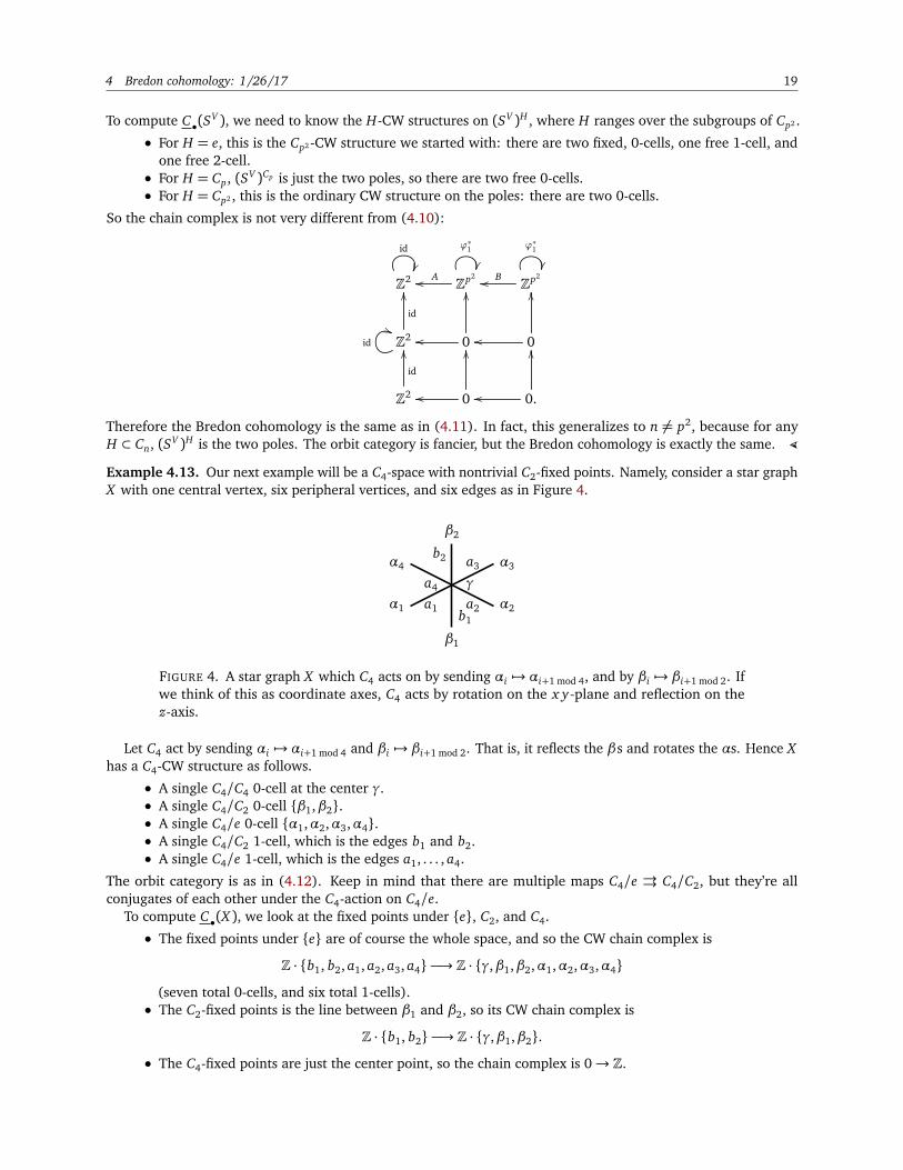
To compute C•(SV ), we need to know the H-CW structures on (SV )H , where H ranges over the subgroups of Cp2 .
• For H = e, this is the Cp2 -CW structure we started with: there are two fixed, 0-cells, one free 1-cell, andone free 2-cell.
• For H = Cp, (SV )Cp is just the two poles, so there are two free 0-cells.• For H = Cp2 , this is the ordinary CW structure on the poles: there are two 0-cells.
So the chain complex is not very different from (4.10):
Z2
id
Zp2Aoo
ϕ∗1
Zp2Boo
ϕ∗1
Z2
id
OO
id((
0oo
OO
0oo
OO
Z2
id
OO
0oo
OO
0.oo
OO
Therefore the Bredon cohomology is the same as in (4.11). In fact, this generalizes to n 6= p2, because for anyH ⊂ Cn, (SV )H is the two poles. The orbit category is fancier, but the Bredon cohomology is exactly the same. (
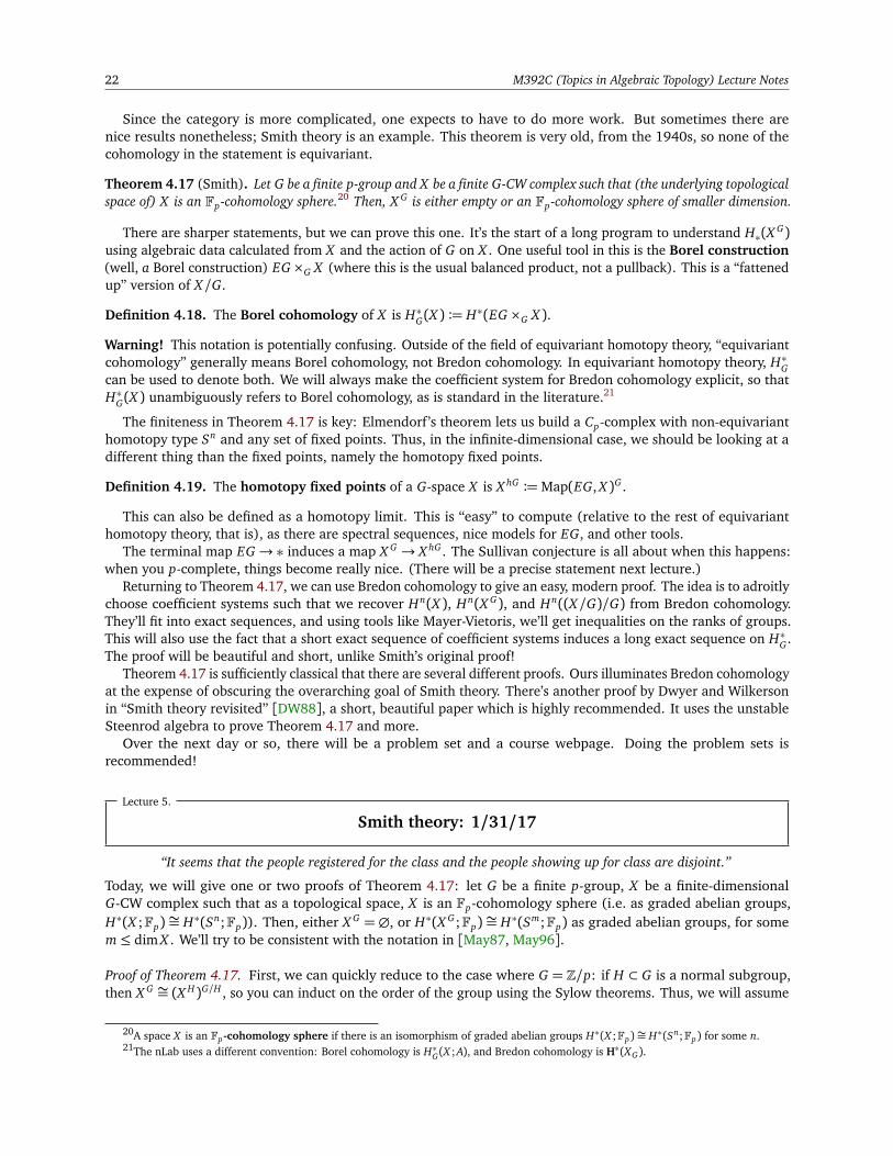
Example 4.13. Our next example will be a C4-space with nontrivial C2-fixed points. Namely, consider a star graphX with one central vertex, six peripheral vertices, and six edges as in Figure 4.
α3
α2
α4
α1
a3
a2
a4
a1
β2
β1
b2
b1
γ
FIGURE 4. A star graph X which C4 acts on by sending αi 7→ αi+1 mod 4, and by βi 7→ βi+1 mod 2. Ifwe think of this as coordinate axes, C4 acts by rotation on the x y-plane and reflection on thez-axis.
Let C4 act by sending αi 7→ αi+1 mod 4 and βi 7→ βi+1 mod 2. That is, it reflects the βs and rotates the αs. Hence Xhas a C4-CW structure as follows.
• A single C4/C4 0-cell at the center γ.• A single C4/C2 0-cell β1,β2.• A single C4/e 0-cell α1,α2,α3,α4.• A single C4/C2 1-cell, which is the edges b1 and b2.• A single C4/e 1-cell, which is the edges a1, . . . , a4.
The orbit category is as in (4.12). Keep in mind that there are multiple maps C4/e ⇒ C4/C2, but they’re allconjugates of each other under the C4-action on C4/e.
To compute C•(X ), we look at the fixed points under e, C2, and C4.
• The fixed points under e are of course the whole space, and so the CW chain complex is
Z · b1, b2, a1, a2, a3, a4 −→ Z · γ,β1,β2,α1,α2,α3,α4
(seven total 0-cells, and six total 1-cells).• The C2-fixed points is the line between β1 and β2, so its CW chain complex is
Z · b1, b2 −→ Z · γ,β1,β2.
• The C4-fixed points are just the center point, so the chain complex is 0→ Z.

20 M392C (Topics in Algebraic Topology) Lecture Notes
With bases for chain groups as above, the differentials are
dC4=
−1 −1 −1 −1 −1 −11 00 1
1 0 0 00 1 0 00 0 1 00 0 0 1
and dC2=
−1 −11 00 1
,
i.e. C•(X ) is
Z6C4
((Z7
dC4oo C4
vv
Z3C2
(( ?
OO
Z2?
OO
dC2oo C2
vv
Z?
OO
0.oo
OO
The C4-actions in the top row are the regular C4-representation on the subspace generated by the αi or the edgesthey touch. Similarly, the C2-actions in the middle row are the regular representations on the subspaces generatedby the β j and their edges. The inclusions in the diagram Zk ,→ Zm are as the first k components.
Applying Hom(–,Z), we get a cochain complex
Z3
−1 1 0−1 0 1
// Z2.
so the cohomology is that of a point, which is reassuring. (
Example 4.14. Let’s compute Bredon cohomology with coefficients in a non-constant coefficient system. For C2,this is the data of an abelian group A, an involution ϕ : A→ A, and a map Z→ A equivariant with respect to ϕ. Forexample, let’s take Z[i] with ϕ acting by complex conjugation, and call this coefficient system M . system.
Let C2 act on S2 by reflection across a meridian m; this is the representation sphere S1+σ. It has a C2-CWstructure as follows.
• One 0-cell e of the form C2/C2 × D0 at the north pole.• One 1-cell f of the form C2/C2 × D1, which is the meridian m.• One 2-cell g of the form C2/e× D2, which is everything else.
TODO: add picture.Let g1 and g2 denote the two nonequivariant 2-cells that make up g. Then, orient f and g such that ∂ f = e−e = 0
and ∂ g1 = ∂ g2 = f .Then, C•(S
1+σ) is
Z · e
id
Z · f
id
0oo Z · g1, g2
swap
(1 1 )oo
Z · e
id
OO
Z · f0oo
id
OO
0.oo
OO
Now we map to M . We have two copies of Hom(Z, M) = Z, and at degree 2 we get HomZ[C2](Z[C2],Z[i]), whichis free of rank 2. The cochain complex is
Z 0 // Z rank 1 // Z2,
so the Bredon cohomology is
HkC2(S1+σ; M) =
¨
Z, k = 0,2
0, otherwise.(

4 Bredon cohomology: 1/26/17 21
We want cohomology to have nice formal properties analogous to the Eilenberg-Steenrod axioms. We’ll think ofHG as a general G-equivariant cohomology theory of pairs Hn
G(X , A; M), but in our case this will just be HnG(X/A; M).
(1) H∗G should be invariant under weak equivalences: a weak equivalence X → Y should induce an isomor-
phism HnG(Y ; M)
∼=−→HnG(X ; M).
(2) Given a pair A⊆ X , we get a long exact sequence
· · · // HnG(X , A; M) // Hn
G(X ; M) // HnG(A; M) δ // Hn+1(X , A; M) // · · ·
(3) The excision axiom: if X = A∪ B, then
HnG(X/A; M)∼= Hn
G(B/(A∩ B); M).
(4) The Milnor axiom:
HnG
∨
i
X i; M
=∏
i
HnG(X i; M).
(5) Finally, for now we impose the dimension axiom: our points are orbits G/J , so we ask that Hn(G/H; M)is concentrated in degree 0.
Some of these are easier than others: Bredon cohomology is manifestly homotopy-invariant in the same ways asordinary cohomology, so invariance under weak equivalence and the Milnor axiom are immediate, and excisionfollows because if all spaces involved are CW complexes, X/A∼= B/(A∩ B).
What takes more work is the dimension axiom and the long exact sequence. We’ll show that Cn(X ) is a projectiveobject, and hitting projective objects with Hom produces a long exact sequence by homological algebra. (Recallthat an object P in a category where you can do homological algebra is projective if Hom(P, –) is exact, which isequivalent to maps to P lifting across surjections M P.)
Proof of the dimension and long exact sequence axioms. Observe that Cn(X ) splits as a direct sum of pieces Hn(G/H+∧Sn)∼= eH0(G/H) indexed by the cells G/H of X . At G/K , H0(G/H) = Z[π0(G/H)K]. This is a free abelian group,and we’ll directly use the lifting criterion to prove this is projective. That is, we’ll write down an isomorphism
ϕ : HomFun(O opG ,Ab)(H0(G/H), M)
∼=−→M(G/H).
This immediately proves H0(G/H) is projective: evaluating a coefficient system on an exact sequence produces anexact sequence, and we’ve shown Hom(H0(G/H), –) is evaluation of a coefficient system.
The map ϕ takes a homomorphism θ and applies it to idG/H , which produces something in M(G/H). Why isthis an isomorphism? The Yoneda lemma is a fancy answer, but you can prove it in a more elementary manner.
Exercise 4.15. Calculate that any θ ∈ HomFun(O opG ,Ab)(H0(G/H), M) is determined by where the identity id ∈
MapOG(G/H, G/H) is sent, implying ϕ is an isomorphism.
Thus, we’ve effectively calculated the value at G/H, proving the dimension axiom as well.
The Eilenberg-Steenrod axioms hold for Bredon homology, and the proof is the same.
Remark. Let’s foreshadow a little bit. In ordinary homotopy theory, one can show that the Eilenberg-Steenrodaxioms plus the value on points determine a cohomology theory, and this is still true in the equivariant case. Butthen one wonders about Brown representability and what happens when you remove the dimension axiom — andindeed there are lots of interesting examples of generalized equivariant cohomology theories. (
Exercise 4.16. We constructed a functor H : Fun(O opG ,Top)→ Fun(O op
G ,Ab). Show that HM represents HnG(–; M).
This slick definition of H is one of the advantages of working with presheaves on the orbit category.
Remark. You might also want to have a universal coefficient sequence, but it’s more complicated. The short exactsequence in ordinary homotopy theory depends on the existence of short projective resolutions. Here, we haveenough projectives and injectives, but resolutions are longer. Thus, taking an injective resolution of M and filteringthe resulting double complex, one obtains a spectral sequence
Extp,q(C∗(X ), M) =⇒ H p+qG (X ; M).
Warning: indexing might be slightly off.There’s a corresponding Tor spectral sequence. (
22 M392C (Topics in Algebraic Topology) Lecture Notes
Since the category is more complicated, one expects to have to do more work. But sometimes there arenice results nonetheless; Smith theory is an example. This theorem is very old, from the 1940s, so none of thecohomology in the statement is equivariant.
Theorem 4.17 (Smith). Let G be a finite p-group and X be a finite G-CW complex such that (the underlying topologicalspace of) X is an Fp-cohomology sphere.20 Then, X G is either empty or an Fp-cohomology sphere of smaller dimension.
There are sharper statements, but we can prove this one. It’s the start of a long program to understand H∗(X G)using algebraic data calculated from X and the action of G on X . One useful tool in this is the Borel construction(well, a Borel construction) EG×G X (where this is the usual balanced product, not a pullback). This is a “fattenedup” version of X/G.
Definition 4.18. The Borel cohomology of X is H∗G(X ) := H∗(EG ×G X ).
Warning! This notation is potentially confusing. Outside of the field of equivariant homotopy theory, “equivariantcohomology” generally means Borel cohomology, not Bredon cohomology. In equivariant homotopy theory, H∗Gcan be used to denote both. We will always make the coefficient system for Bredon cohomology explicit, so thatH∗G(X ) unambiguously refers to Borel cohomology, as is standard in the literature.21
The finiteness in Theorem 4.17 is key: Elmendorf’s theorem lets us build a Cp-complex with non-equivarianthomotopy type Sn and any set of fixed points. Thus, in the infinite-dimensional case, we should be looking at adifferent thing than the fixed points, namely the homotopy fixed points.
Definition 4.19. The homotopy fixed points of a G-space X is X hG :=Map(EG, X )G .
This can also be defined as a homotopy limit. This is “easy” to compute (relative to the rest of equivarianthomotopy theory, that is), as there are spectral sequences, nice models for EG, and other tools.
The terminal map EG→ ∗ induces a map X G → X hG . The Sullivan conjecture is all about when this happens:when you p-complete, things become really nice. (There will be a precise statement next lecture.)
Returning to Theorem 4.17, we can use Bredon cohomology to give an easy, modern proof. The idea is to adroitlychoose coefficient systems such that we recover Hn(X ), Hn(X G), and Hn((X/G)/G) from Bredon cohomology.They’ll fit into exact sequences, and using tools like Mayer-Vietoris, we’ll get inequalities on the ranks of groups.This will also use the fact that a short exact sequence of coefficient systems induces a long exact sequence on H∗G .The proof will be beautiful and short, unlike Smith’s original proof!
Theorem 4.17 is sufficiently classical that there are several different proofs. Ours illuminates Bredon cohomologyat the expense of obscuring the overarching goal of Smith theory. There’s another proof by Dwyer and Wilkersonin “Smith theory revisited” [DW88], a short, beautiful paper which is highly recommended. It uses the unstableSteenrod algebra to prove Theorem 4.17 and more.
Over the next day or so, there will be a problem set and a course webpage. Doing the problem sets isrecommended!
Lecture 5.
Smith theory: 1/31/17
“It seems that the people registered for the class and the people showing up for class are disjoint.”
Today, we will give one or two proofs of Theorem 4.17: let G be a finite p-group, X be a finite-dimensionalG-CW complex such that as a topological space, X is an Fp-cohomology sphere (i.e. as graded abelian groups,H∗(X ;Fp) ∼= H∗(Sn;Fp)). Then, either X G = ∅, or H∗(X G;Fp) ∼= H∗(Sm;Fp) as graded abelian groups, for somem≤ dim X . We’ll try to be consistent with the notation in [May87, May96].
Proof of Theorem 4.17. First, we can quickly reduce to the case where G = Z/p: if H ⊂ G is a normal subgroup,then X G ∼= (X H)G/H , so you can induct on the order of the group using the Sylow theorems. Thus, we will assume
20A space X is an Fp-cohomology sphere if there is an isomorphism of graded abelian groups H∗(X ;Fp)∼= H∗(Sn;Fp) for some n.21The nLab uses a different convention: Borel cohomology is H∗G(X ; A), and Bredon cohomology is H∗(XG).
5 Smith theory: 1/31/17 23
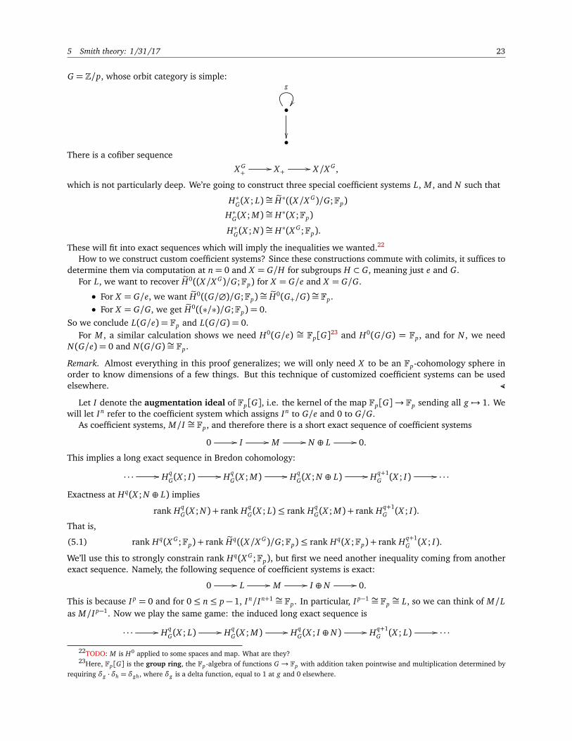
G = Z/p, whose orbit category is simple:
•
g
•
There is a cofiber sequence
X G+
// X+ // X/X G ,
which is not particularly deep. We’re going to construct three special coefficient systems L, M , and N such that
H∗G(X ; L)∼= eH∗((X/X G)/G;Fp)
H∗G(X ; M)∼= H∗(X ;Fp)
H∗G(X ; N)∼= H∗(X G;Fp).
These will fit into exact sequences which will imply the inequalities we wanted.22
How to we construct custom coefficient systems? Since these constructions commute with colimits, it suffices todetermine them via computation at n= 0 and X = G/H for subgroups H ⊂ G, meaning just e and G.
For L, we want to recover eH0((X/X G)/G;Fp) for X = G/e and X = G/G.
• For X = G/e, we want eH0((G/∅)/G;Fp)∼= eH0(G+/G)∼= Fp.• For X = G/G, we get eH0((∗/∗)/G;Fp) = 0.
So we conclude L(G/e) = Fp and L(G/G) = 0.For M , a similar calculation shows we need H0(G/e) ∼= Fp[G]
23 and H0(G/G) = Fp, and for N , we needN(G/e) = 0 and N(G/G)∼= Fp.
Remark. Almost everything in this proof generalizes; we will only need X to be an Fp-cohomology sphere inorder to know dimensions of a few things. But this technique of customized coefficient systems can be usedelsewhere. (
Let I denote the augmentation ideal of Fp[G], i.e. the kernel of the map Fp[G]→ Fp sending all g 7→ 1. Wewill let In refer to the coefficient system which assigns In to G/e and 0 to G/G.
As coefficient systems, M/I ∼= Fp, and therefore there is a short exact sequence of coefficient systems
0 // I // M // N ⊕ L // 0.
This implies a long exact sequence in Bredon cohomology:
· · · // HqG(X ; I) // Hq
G(X ; M) // HqG(X ; N ⊕ L) // Hq+1
G (X ; I) // · · ·
Exactness at Hq(X ; N ⊕ L) implies
rank HqG(X ; N) + rank Hq
G(X ; L)≤ rank HqG(X ; M) + rank Hq+1
G (X ; I).
That is,
(5.1) rank Hq(X G;Fp) + rank eHq((X/X G)/G;Fp)≤ rank Hq(X ;Fp) + rank Hq+1G (X ; I).
We’ll use this to strongly constrain rank Hq(X G;Fp), but first we need another inequality coming from anotherexact sequence. Namely, the following sequence of coefficient systems is exact:
0 // L // M // I ⊕ N // 0.
This is because I p = 0 and for 0≤ n≤ p− 1, In/In+1 ∼= Fp. In particular, I p−1 ∼= Fp∼= L, so we can think of M/L
as M/I p−1. Now we play the same game: the induced long exact sequence is
· · · // HqG(X ; L) // Hq
G(X ; M) // HqG(X ; I ⊕ N) // Hq+1
G (X ; L) // · · ·
22TODO: M is H0 applied to some spaces and map. What are they?23Here, Fp[G] is the group ring, the Fp-algebra of functions G → Fp with addition taken pointwise and multiplication determined by
requiring δg ·δh = δgh, where δg is a delta function, equal to 1 at g and 0 elsewhere.
24 M392C (Topics in Algebraic Topology) Lecture Notes
which impliesrank Hq
G(X ; N) + rank HqG(X ; I)≤ rank Hq
G(X ; M) + rank Hq+1G (X ; L),
i.e.
(5.2) rank Hq(X G;Fp) + rank HqG(X ; I)≤ rank Hq(X ;Fp) + rank Hq+1((X/X G)/G;Fp).
Let’s use this to prove
(5.3) rank eHq((X/X G)/G;Fp) +q+r∑
i=q
rank H i(X G;Fp)≤ rank eHq+r+1 +q+r∑
i=q
rank H i(X ;Fp).
Let
aq := rank Hq(X G;Fp)
bq := rank Hq(X ;Fp)
cq := rank Hq((X/X G)/G;Fp)
dq := rank HqG(X ; I).
Then, (5.1) and (5.2) sayaq + cq ≤ bq + dq+1 and aq + dq ≤ bq + cq+1.
Now, adding (5.1) for q even and (5.2) for q odd proves (5.3).When q = 0 and r is large, the finite-dimensionality of X implies that
(5.4)∑
i
rank H i(X G;Fp)≤∑
i
rank H i(X ;Fp).
This is already an interesting bound, especially relative to the amount of work we’ve put in.Specializing to X an Fp-cohomology sphere, (5.4) means
∑
i
rank H i(X G;Fp)≤ 2.
We want to show this sum isn’t 1 (so that we get the cohomology of a sphere) and that the top nonzero rank is atmost n. We will do this with another short exact sequence of coefficient systems:
0 // In+1 // In // L // 0.
From this, we get another long exact sequence. Applying the Euler characteristic, we obtain that
(5.5) χ(X ) = χ(X G) + peχ((X/X G)/G).
Hereeχ(Y ) :=
∑
i
(−1)i rank eH i(Y )
is the reduced Euler characteristic.Equation (5.5) already implies that χ(X )≡ χ(X G)mod p, so
∑
rank H∗(X G;Fp) 6= 1 in our case.
Exercise 5.6.(1) Think about choices of q and r that allow you to deduce m≤ n, finishing the proof.(2) Small changes need to be made to this argument when p = 2; what are they?
This is an appealing proof: some fairly simple calculations and a dash of formal theory very effectively led tothe result. We’ll give another proof with different advantages and disadvantages.
Smith theory naturally leads to questions about how to recover H∗(X G) algebraically from some equivariantcohomology theory on X . Last time, we introduced Borel cohomology H∗G(X ) := H∗(EG ×G X ), where EG is a freeG-space that’s nonequivariantly contractible (which is simple to construct with the bar construction or throughElmendorf’s theorem).
In the following, all cohomology is understood to have coefficients in Fp. Recall that the Bredon cohomologyof X is defined to be H∗G(X ) := H∗(EG ×G X ). For a subgroup H ⊂ G, let SH ⊂ H∗(BG) be the multiplicativeset generated by the classes in H2(BG) that are images of the Bockstein homomorphism H1(BG)→ H2(BG) ofthe elements that are nontrivial in H1(BH). This uses the fact that Borel cohomology is an H∗(BG)-module:H∗(EG ×G ∗)∼= H∗(EG/G) = H∗(BG), and using the terminal map X → ∗ we get a map H∗(BG)→ H∗(EG ×G X ).
6 Smith theory: 1/31/17 25
Theorem 5.7. Let G be a finite p-group and H ⊂ G be a subgroup. Then, there is an isomorphism S−1H H∗G(X )
∼=→S−1
H H∗G(XH).
There’s a rich theory of unstable modules over the Steenrod algebra Ap, which could fill a whole semester.There’s a functor Un which produces unstableAp-modules, in a sense by only keeping the unstable part.
Theorem 5.8 (Dwyer-Wilkerson [DW88]).
H∗(X G)∼= Fp ⊗H∗(BG) Un(S−1G H∗(EG ×G X )).
The proof uses arguments that were hard to think of, but easy to follow.We’ll use these theorems to prove Smith’s theorem using the Serre spectral sequence for
X // EG ×G X // BG.
This will be the nicest kind of spectral sequence argument: everything degenerates.Theorem 5.7 is an example of a general class of localization theorems in equivariant cohomology. In these
theorems, one considers the fiber sequence X G+ → X+ → X/X G , and wants to show that for some functor E,
E(X G+ )∼= E(X+). This boils down to showing E(X/X G) vanishes, which will always follow from showing that E
vanishes on G-spaces whose G-actions are free away from the basepoint. In general, this will reduce to consideringcells, so one considers E(G/H+ ∧
∨
α Sqα) for some wedge of spheres.In our case, E(G/H+ ∧
∨
α Sqα) is
S−1H H∗G
G/H+ ∧∨
α
Sqα
= S−1H H∗
EG ×G
G/H+ ∧∨
α
Sqα
Now, the term EG ×G G/H ∼= EG/H ∼= BH, so we have a piece that looks like H∗(BH), which is how BH insertsitself into the argument.
Exercise 5.9. Finish the Serre spectral sequence proof of Theorem 4.17. Hint: there’s a simple geometric reasonwhy the spectral sequence collapses, which is what makes this whole thing go.
Soon we’ll start talking about the stable category. As preparation for this, if you don’t already know it, it’s goodto remind yourself of it.
The Q&A session will be Thursday at 8:30 PM.
Lecture 6.
The localization theorem and the Sullivan conjecture: 2/2/17
“The number of children he had was a monotonically increasing function.”There are three goals in today’s lecture.
(1) We’ll discuss the localization theorem (Theorem 5.7) again, and prove it, providing a bit more context forwhere it came from.
(2) We’ll talk about the Sullivan conjecture (Theorem 6.5). This is really Sullivan’s attack on Adams’ conjecture,and is a very important story. We won’t prove the conjecture, because it’s hard, but the context around itwas a major motivation for a lot of the work in algebraic and geometric topology in the past 40 years.Sullivan wrote up some notes for a class of his at MIT, which have been published as [Sul05], and youshould read them: they are enlightening and contain all of the jokes he told in class!
(3) We’ll introduce the stable category, discussing Spanier-Whitehead duality and the Pontrjagin-Thomconstruction. If you want points (orbits) to have Spanier-Whitehead duals, you’re inexorably forced toconstruct this stable category.
The localization theorem. Recall that the Borel cohomology H∗(EG ×G X ) is an H∗(BG)-module, through themap EG×G X → EG×G ∗ = BG. Thus, we should compute H∗(BG) as a ring. In the case we care about, G = (Z/p)n;let’s start with n= 1.
There’s a nice geometric model for BZ/p as an “infinite-dimensional lens space:” let S∞ denote the unitsphere in an infinite-dimensional complex Hilbert space,24 and give it a Cp-action by z 7→ e2πi/pz. Then, theinfinite-dimensional lens space is S∞/Cp.
24Alternatively, you could choose S∞ to be the colimit of Sn for all n, through the inclusion Sn ,→ Sn+1 at the equator. These two choicesare not homeomorphic, but produce homotopy equivalent models of BZ/p.
26 M392C (Topics in Algebraic Topology) Lecture Notes
The quotient S∞ S∞/Cp is a covering map, and S∞ is contractible. The proof goes through some version ofthe Eilenberg swindle:
• There is a homotopy from idS∞ to s : (x1, x2, . . . ) 7→ (0, x1, x2, . . . ). In fact, it’s a straight-line homotopy.• There is a straight-line homotopy from s to (0, x1, . . . ) 7→ (1,0, 0, . . . ).
Thus S∞/Cp is the quotient of a contractible space by a free G-action, so it deserves to be called BZ/p.You can set up a cell structure on BZ/p as with finite-dimensional lens spaces, and therefore compute that
Hk(BZ/p)∼=
¨
Z/p, k even
0, k odd.
Using the universal coefficient theorem, you can then deduce that
Hk(BZ/p;Z/p)∼= Z/p
for all k. Now we want to deduce the ring structure.Recall that if
0 // M // L // N // 0is a short exact sequence, it induces a long exact sequence in cohomology:
· · · // Hk(–; M) // Hk(–; L) // Hk(–; N)β // Hk+1(–; M) // · · ·
Let’s apply this to the short exact sequences
0 // Z·p //
Z //
Z/p //
0
0 // Z/p·p // Z/p2 // Z/p // 0.
This is a map of short exact sequences, inducing a map of their long exact sequences.
(6.1)
· · · // Hq(X ;Z) //
Hq(X ;Z) //
Hq(X ;Z/p) //
Hq+1(X ;Z) //
· · ·
· · · // Hq(X ;Z/p) // Hq(X ;Z/p2) // Hq ∗ (X ;Z/p)β // Hq+1(X ;Z/p) // · · ·
The map β : Hq(X ;Z/p)→ Hq+1(X ;Z/p) will be called the Bockstein homomorphism, and is a simple exampleof a cohomology operation.
We now assume p is odd.
Lemma 6.2. If n is odd, the Bockstein for BZ/p is an isomorphism; if n is even, it’s 0.
Proof. First, observe that the diagram
Hn(BZ/p;Z)f // Hn(BZ/p;Z/p)
g //
β ((
Hn+1(BZ/p;Z)
π
// Hn+1(BZ/p;Z)
Hn+1(BZ/p;Z/p)
commutes, and the top row is exact.• If n is even, f is an isomorphism, so g = 0, so β = 0.• if n is odd, g and π are surjections, so β is a surjection between two Fp-vector spaces of the same rank, soβ is an isomorphism.
Next, a nice way to compute the cup product. The map BZ/p→ CP∞ is cellular, and is a homeomorphismwhen restricted to even-dimensional cells. As the cell structure determines the cup product structure, the cupproducts on Heven(BZ/p;Z/p) and Heven(CP∞; BZ/p)∼= Z/p[y1] agree. On the odd-dimensional cells, the cupproduct is graded commutative rather than strictly commutative, so we get an exterior algebra. Therefore weconclude that
H∗(BZ/p;Z/p)∼= Λ(x1)⊗Z/p[y1],

6 The localization theorem and the Sullivan conjecture: 2/2/17 27
where |x1|= 1, |y1|= 2, and β x1 = y1.By essentially the same argument, one can compute the cohomology ring for B(Z/p)n.
Proposition 6.3. As rings, there is an isomorphism
H∗(B(Z/p)n;Z/p)∼= Λ(x1, . . . , xn)⊗Z/p[y1, . . . , yn],
where β x i = yi .
Exercise 6.4. Figure out the slight changes needed for p = 2.
Recall that the localization theorem asserted that if G is a finite p-group, S−1H H∗(EG×G X )∼= S−1
H H∗(EG×G X G),where S is the multiplicative system generated by images of the Bockstein homomorphism in H∗(BG;Z/p). We’llprove this in the case when G is abelian.
We mentioned last time that it’s possible to inductively reduce to considering H∗(BH)⊗ H∗∨
Sqi
. It’s nowclear25 that something in S restricts to 0 in H∗(BH), completing the proof (in the abelian case).
The localization fails terribly for infinite nonabelian compact Lie groups G. For example, for any topologicalspace K , there exists a G-CW complex X such that X is nonequivariantly contractible, X is finite-dimensional, andX G ' K .
The Sullivan conjecture.
Theorem 6.5 (Sullivan conjecture). Let G be a finite, abelian p-group. Then, X hG → X G is an equivalence onp-completions.
Recall that X hG := Map(EG, X )G , so this asserts a weak equivalence (after p-completing) Map(EG, X )G →Map(∗, X )G .
By p-completion, we mean Bousfield localization at Fp cohomology. This produces the category of spaces whereequivalences are detected by H∗(–;Fp). The most familiar example of completion is rationalization, a localizationwhere equivalences are detected by rational homotopy groups, and one of Sullivan’s biggest achievements wasproviding a completely algebraic description of the rational homotopy category in [Sul77]. More broadly, he hadthe insight that to study a problem in homotopy theory, one could localize at Q and at each Fp and study eachpiece, which has been a very fruitful approach.
p-completion falls into the collection of basic life skills for homotopy theorists, so if you haven’t seen it before,you should read about it. The standard reference is [BK72b], but this is 500 pages and hard to read.
Sullivan’s conjecture is an algebro-geometric attack on the Adams conjecture. This was within Sullivan’s programto find algebraic models of manifolds. This is still being done today, and is what led Sullivan to think about stringtopology and related things.
Let X be a manifold. We first have the homotopical data of X , C∗(X ;Q) and C∗(X ;Fp), which are “commutativerings.”26 That X is a manifold means we can see Poincaré duality, which doesn’t appear in all E∞ dg algebras. Butwe still need some way to encode additional geometric obstructions, e.g. a way to encode the tangent and normalbundles.
It’s been an interesting, but as yet unsuccessful, attack to use a Frobenius algebra structure to try to obtain thisgeometric data. It’s neat to think about what the E∞ analogue of a Frobenius algebra is, and this is intimatelyrelated to Lurie’s approach to the cobordism hypothesis [Lur09], thinking about fully dualizable objects in asymmetric monoidal∞-category.
This circle of ideas is also related to surgery theory; there’s been lots of cool work by smart people in it, andL-theory was invented basically as an algebraic home for these geometric objects.
Sullivan was interested in the Adams conjecture because it says that one can identify the tangent bundle insideK-theory K(X ) with its Adams operations ψk, as fiberwise homotopy types.
Sullivan’s idea, motivated by Quillen, was to use the theory of étale homotopy types. This translates somequestions about scheme theory into homotopy theory. For example, if X is a variety (more generally a scheme),one can assign some profinite topological object, built out of something like a system of hypercovers.27 So ifyou take the profinite completion of the complex points X (C)∧, it has an action of the absolute Galois groupGal(Q/Q)— and another crazy interpretation of the Adams conjecture is that the profinite completion of K(X )
25TODO: I didn’t follow this proof in class.26They’re not literally commutative; instead, they’re E∞ dg algebras. They also have more structure as modules over the Steenrod algebra.27If you don’t know what this is, it’s an example of an extremely interesting construction which you should look up sometime.

28 M392C (Topics in Algebraic Topology) Lecture Notes
can be interpreted in this way, and has an action of (bZ)∗ (bZ is the Galois group of the maximal abelian extensionover Q). The conjecture is that this action is by the Adams operations.
There’s a deep and inadequately understood story (which could be an opportunity for you) connecting p-adicallycompleted complex K-theory KU∧p to number theory, specifically the Iwasawa algebra. Adams noticed this, but it’stoo interesting to be a coincidence.
Anyways, stable fiberwise homotopy types are invariant under this (bZ)∗-action, which led Sullivan to askquestions about (X (C)∧)hC2 versus X (R)∧. The references [Sul05, Sul74] are both excellent for this.
For reasons of scope, we can’t go into too much more detail, but you should definitely look this stuff up.The takeaway is that equivariant homotopy theory has been motivated by seemingly unrelated questions aboutmanifolds. There’s been a lot of interesting interplay between algebraic and geometric topology in the last halfcentury, and this is one of the cites of contact.
The stable category and stable phenomena. There are lots of ways to think about where stabilization comesfrom.
(1) The Freudenthal suspension theorem says that if X is nondegenerately based (meaning the based inclusionmap ∗ ,→ X is a cofibration) and n−1-connected, then πq(X )→ πq+1(ΣX ) is an isomorphism for q < 2n−1and a surjection when q = 2n−1.28 It’s easier to see that cohomology groups are stable under suspension,but this tells us that homotopy groups stabilize in a range that increases at about twice the rate thatthe connectivity of X does. Since ΣnX is at least n-connected, this suggests you could replace X by thesequence X ,ΣX , . . . ,ΣnX , . . . , and keep track of that instead, regarding it as a repository for the stablehomotopy groups πS
n(X ) := colimkπn+k(ΣkX ). One way to think of this is as formally making homotopytheory into a homology theory (which it isn’t a prioiri); you end up taking the same kind of colimit.
You could do this equivariantly: we have representation spheres. But it’s not entirely clear what to do.(2) Another perspective is that the stable category is the result of inverting the canonical map29
(6.6)k∨
i=1
X →k∏
i=1
X .
Again, this is something you can think about making precise; the stable category is the initial triangulatedcategory constructed from Top in which (6.6) is an isomorphism. In particular, this forces the homotopycategory to be additive.
Again, we could do this equivariantly.(3) Suppose we have a functor F from finite CW complexes to Top such that F(∗) = ∗, and suppose F
commutes with filtered colimits and preserves weak equivalences (e.g. if it’s topologically or simpliciallyenriched, for formal reasons). By taking colimits, we can obtain a functor bF from CW complexes to Top.We say F is excisive if it takes pushouts to pullbacks; this is an old perspective, which was used to showthe Dold-Thom theorem, that the infinite symmetric product SP∞ is a cohomology theory. In any case, ifF is excisive, F(Sn) represents a cohomology theory. Namely, the homotopy pushout
Sn //
Dn+1
Dn+1 // Sn+1
creates suspension, and via F , becomes a pullback creating Ω. Asking what the excisive functors are leadsto the stable category, and is also something you could do equivariantly.
(4) Another perspective: what is the Spanier-Whitehead dual of a point? Taking shifts, what’s the Spanier-Whitehead dual of Sn? Equivariantly, one wants to know the Spanier-Whitehead duals of G/H+. Thisis important for defining Poincaré duality, etc. Nonequivariantly, the best way to answer this is thePontrjagin-Thom construction, which not only answers this, but provides a deep understanding for whatthe stable homotopy groups of the spheres are. We’ll do this equivariantly next time, and it will tell uswhat the spheres are.
28The map comes from the loop-suspension adjunction, which gives us a unit X → ΩΣX , hence a map ΩqX → Ωq+1ΣX , and the map onhomotopy groups is π0 of that map. This is the based version of the mapping space and Cartesian product adjunction: ΣX := S1 ∧ X andΩX :=Map(S1, X ) are adjoint functors.
29The existence of this map follows from the universal property of the product.

7 The localization theorem and the Sullivan conjecture: 2/2/17 29
There’s a choice here: you could just say “let’s take the category of orthogonal G-spectra,” but having somemotivation for why we’re doing and what we’re doing is important.
Lecture 7.
Question-and-answer session: 2/2/17
Question 7.1. So, why does anyone care about Spanier-Whitehead duality?
One answer is that Spanier-Whitehead duality formally implies Poincaré duality. Poincaré duality is a remarkablefact about the cohomology of manifolds, which is one good reason to care.
Another is that it’s the real setting for the Euler characteristic — really. The Euler characteristic arises as a trace,and therefore some kind of categorical duality should appear.
Being more specific, let’s consider a closed symmetric monoidal category C with unit S (so secretly we’rethinking of the stable homotopy category). Spanier-Whitehead duality consists of two maps ε : X ∧ Y → S andM : S→ X ∧ Y , such that the composition
X ∼= S∧ X M∧id // X ∧ Y ∧ Xid∧(ετ)// X ∧ S∼= X
is the identity.Using an adjunction, you can show X ∼= F(Y,S) and Y ∼= F(X ,S), and so X is the dual of its dual. This has lots
of formal consequences, including Poincaré duality, the construction of things such as the Euler characteristic, andmore. The Spanier-Whitehead dual of X is often denoted DX .
Suppose that we’re in an algebraic category, say HQ-module spectra (the rational stable homotopy category).Then, HQ is the unit, so DX = C∗(X ;Q) (maps from X to Q). That is, the Spanier-Whitehead dual embeds theunstable homotopy theory of X , as long as you remember the E∞-ring structure on DX (which is bizarre, e.g. it’snot connective). There’s a quite nontrivial theorem that E∞ maps between DX and DY correspond to maps ofspaces between X and Y .
This sort of data is useful for algebraicizing manifolds, and that would be nice for classifying manifolds, agoal with fairly broad applications outside of homotopy theory. And Spanier-Whitehead duality has importantconsequences on this: Sullivan began it by showing [Sul77] that the E∞-ring structure on C∗(X ;Q) controls therationalization XQ, and Mandell [Man01] ended it by showing that the E∞ structure on C∗(X ;Fp) controls X∧p .
Question 7.2. What are some of the obstacles to extending equivariant homotopy theory to groups that aren’tcompact Lie groups?
One cornerstone of homotopy theory is the Pontrjagin-Thom construction, which depends on the weak Whitneyembedding theorem: that a manifold can be embedded in some high-dimensional RN . This still works equivariantlybut only for compact Lie groups — a G-manifold X can be embedded in some high-dimensional G-representation.This is again an important piece in the equivariant Pontrjagin-Thom construction, and its failure for noncompactgroups is one major reason things don’t work. There are other things that require compactness (e.g. descendingchain arguments). People have tried and not gotten anywhere.
In stable homotopy theory, there’s a modification of the orbit category into something called the Burnsidecategory, and we’ll see that it controls a lot of the stable homotopy theory of G-spaces. In fact, if you have somethingthat strongly resembles the Burnside category, you have something that looks like equivariant stable homotopytheory. Clark Barwick and his collaborators have been working on studying presheaves on things that look likeBurnside categories.
A lot of it boils down to the fact that compact Lie groups have a tractable representation theory.
Question 7.3. Recall EF , the classifying space for a family of subgroups. What is it used for?
If you want to focus attention on a family of subgroups, you play with EF . One common example is S1-spaces,in which there are many constructions that are fixed by the finite subgroups of S1, so having that family F ishelpful, and for this one can smash with EF .
There are various other applications. One is called isotropy separation, which splits up F into pieces that canbe detected with different kinds of isotropy subgroups, and one can induct on this in nice cases.
Question 7.4. What does it mean that K-theory and the Adams operations determine the tangent bundle?

30 M392C (Topics in Algebraic Topology) Lecture Notes
It’s a somewhat implicit statement: any possible algebraic statement about the tangent bundle can be translatedinto an equivalent statement in K(X ) that uses the Adams operations.
Question 7.5. How many notions of G-spectra are there?
One way you talk about equivariant stable homotopy theory is a universe, a countably infinite-dimensionalinner product space containing the irreducible representations you care about infinitely often. Then, you haveSpanier-Whitehead duality for G/H iff G/H embeds in the universe, and you get different flavors of homotopytheory depending on which universes you use. There are lots of models here — depending on what you mean,spectra objects or diagrams on OG might not be the right thing for naïve spectra; instead, you need transfers, soyou have to consider sheaves on the Burnside category.
The choice of universe also affects which suspensions you invert: if V is in your universe, you can invert ΣV .Of course, there are probably many different point-set models for stable homotopy, but they’ll give you the same
answer.
Question 7.6. Can you go over how to design a coefficient system such that its cohomology is something obtainedfrom X?
For example, let’s try to determine M such that H∗G(X ; M)∼= H∗(X ). The reason it suffices to determine whatM(G/H) is on all closed subgroups H ⊂ G is the dimension axiom!
So if G = Z/p, you can assign M(G/e) := H0(G/e) and M(G/G) := H0(G/G), and the map between them isH0 of the map G/e→ G/G.
Question 7.7. So far, we’ve mostly seen G-equivariant homotopy theory where G is a finite cyclic group. Is thereanything interesting for nonabelian groups, etc?
Part of the problem is that computing examples is not easy, and it gets much harder when you have a complicatedlattice of subgroups. [LMS86] is 500 pages, and there are scarcely any examples, because the computations fornontrivial examples are so hard!
Peter May invented this stuff and set a bunch of grad students to work on it, but there wasn’t a lot of buzz untilCarlsson proved the Segal conjecture, and then again more recently with Hill-Hopkins-Ravenel. So there haven’tbeen a lot of computations, period. If you do make an interesting computation with, say, the monster group, by allmeans write it up!
So for the most part people have studied cyclic groups and S1. There’s been a little discussion of dihedralactions, and some stuff with the symmetric groups.
There’s also some stuff done for profinite groups. This is in some sense easy to set up formally, especiallybecause you mostly care about finite-index subgroups. People who study Galois actions (e.g. Carlsson’s program tolift the Quillen-Lichtenbaum conjecture into this context) care about this.
Question 7.8. So we’ve spent some time looking at EG, a contractible space with a free G-action, and its quotientBG. What things do people do with these objects?
BG is a classifying space for principal G-bundles (and therefore for G = On or Un, also vector bundles of rankn). That is, homotopy classes of maps X → BG are identified with isomorphism classes of principal G-bundles onX . There’s a book by May, “Classifying spaces and fibrations,” which is excellent and goes into great detail on thisstuff. Because BUn classifies complex vector bundles of rank n, it’s used to construct complex K-theory (and samefor BOn and real K-theory).
In our case, smashing with EG is often a way to localize.A third reason to care about this is group cohomology and other purely algebraic stuff. The group cohomology
of G is the cohomology of BG, and there are plenty of applications of group cohomology.So though BG may be infinite-dimensional, it’s very simple homotopically.
Question 7.9. What’s going on with the construction to the right adjoint to the functorψ in the proof of Elmendorf’stheorem? What’s a coend?
Adrian said some stuff here; I wasn’t able to get it down. He motivated the bar construction as the thing whosehomotopy colimits are ordinary colimits, I think?
Anyways, our setup is that we have a presheaf on the orbit category X ∈ Fun(O opG ,Top) and want to produce
a G-space. The right adjoint30 to ψ is the geometric realization of the bar construction B•(X ,OG , M). The30Recall that the left adjoint was evaluation at G/e.

7 Question-and-answer session: 2/2/17 31
bar construction is a generalization of the bar resolution to compute the derived tensor product: the functorM : OG → Top sending G/H to the space G/H is thought of as a “right OG-module;” instead of tensoring a bunchof elements together, we get a bunch of arrows, meaning we can replace with a coproduct. In some sense, it wouldbe nice to take a tensor product with X , but we have to do so in a derived sense, hence the bar construction.
A coend is a functor that behaves like geometric realization: there’s two functors with opposite variance, andyou want to glue along their common edge, just like in geometric realization.
Question 7.10. How did Elmendorf formalize his proof, given that it was done before model categories wereavailable?
He didn’t: Elmendorf’s paper is eminently readable, and simply provides an equivalence of homotopy categories.It was not lifted into model categories unti much later. This stuff was all put into use fairly recently: for example,not that long ago, it was known to experts but not written down that a left Quillen adjoint that’s part of a Quillenequivalence preserves homotopy limits.
Here, someone asked about the Freudenthal suspension theorem, and this led to a digression.
Remark. Modern cryptography depends on some hardness assumptions, that some functions, such as the discretelog in a finite field, are hard to compute (but easy to check answers to). There’s a paper by Impagliazzo [Imp95]which asks what cryptography and security would look like if certain assumptions were false or true, with cutenames for different worlds. Imagine doing that for the Freudenthal suspension theorem — what if the stable rangewere at about n instead of about 2n? What if it were n/2? (
Question 7.11. In non-equivariant rational homotopy theory, there’s a standard, completely algebraic descriptionof the rational homotopy category. Does this also work for the rational equivariant homotopy category?
This is very hard — someone was working on this, but the work actually depended on an incorrect calculation,and some of it had to be redone. There are people working on an algebraic model for rational G-spectra, but thealgebraic models are very complicated.
Question 7.12. We’ve seen that representations of G play a huge role in equivariant homotopy theory; these couldbe thought of as relating to K-theory of BG (e.g. the representation ring RO(G) is KO0(BG)). More generally, doKO(BG) or MO(BG) play a special role “controlling” the G-equivariant stable category?
People certainly care about computing K-theory or bordism of BG. As to whether those control the G-equivariantstable category—that might be true, but I don’t think anything like that has been said.
Question 7.13. This question comes from GitHub: suppose you’re defining a coefficient system M over G = Cp.This is determined by M(Cp/e), M(Cp/Cp), and a map between them. How do you get the map?
The map is determined by functoriality: in the cases we used to prove Theorem 4.17, which is where thisquestion arose, M(Cp/e) and M(Cp/Cp) are both defined to be H0 of something, so the map between them is H0
of the map Cp/e→ Cp/Cp.
Question 7.14. Do you want to talk about the unstable Steenrod functor Un?
You don’t want to know.
Question 7.15. Does Un appear in the theorem as a technical necessity or for deep reasons?
It’s very deep, and there’s a whole theory of unstable modules over the Steenrod algebra. This involves someextra restrictions.
Question 7.16. So how many kids did Denis Sullivan have?
About 7 or 8 by the end of [Sul05]; one is now also a math professor. There are lots of other anecdotes in thenotes: once he was frustrated with some calculations he was doing, so he hurled the book into the Atlantic ocean.While he was on a boat to Oxford.
Question 7.17. Do we have any previews of the Clark school, besides what few things they’ve posted on the arXiv?
They’ve been doing some really hard stuff: the idea is that G-spectra should be presheaves of spectra on Burnsidecategories, or statements like G-spectra being the initial stable G-symmetric monoidal category. . . you know whatthe theorems should be, but the proofs are technical. Riehl-Verity technology should make some of this easier,hopefully.
32 M392C (Topics in Algebraic Topology) Lecture Notes
Question 7.18. What does it mean that “the Spanier-Whitehead dual of a point involves taking shifts?”
We’ve been a little careless about basepoints: this is really the pointed point, so S0; thus, we really should havesaid the Spanier-Whitehead duals of spheres.
Question 7.19. The Fruedenthal suspension theorem requires inclusion of the basepoint to be a cofibration. Ifyou add a disjoint basepoint, is that the case?
Yes. You can think of a cofibration as a slightly weaker version of a closed inclusion. This is no big technicalobstacle: the whisker construction replaces the basepoint with a line segment, so the homotopy theory isunchanged and the other end of the line segment can be a basepoint that’s cofibrantly included.
Question 7.20. What’s a natural example of a genuine G-spectrum of interest?
One is the equivariant sphere spectrum. Thinking of cohomology theories, there’s equivariant K-theory KUG ,different kinds of equivariant bordism, and KR (a genuine equivariant spectrum that’s built from K-theory).
Question 7.21. Is there an equivariant approach to de Rham theory, e.g. starting with manifolds and equivariantdifferential forms?
Rationally, this can work, but integrally there are issues. Relatedly, defining a G-manifold is not too hard, andthere are nice things like the equivariant tubular neighborhood theorem, but there are some subtleties.
Question 7.22. One of the interpretations of the homotopy category of a model category is localization at theweak equivalences. This suggests that one only needs to look at weak equivalences. So if you only specify weakequivalences, do you get a unique model category?
No, you might not get one at all, and if you do, it won’t be unique. What it means is (modulo some scaryset-theoretic issues) that the homotopy theory only depends on the weak equivalences. If you have a category withweak equivalences, you can form the Dwyer-Kan localization, an associated simplicial category, and then takethe associated quasicategory or∞-category. Under some hypotheses, you can then retreat to a model-categoricalstructure. One commonly heard analogy is that a model category is like choosing a basis for a vector space (wherethe basis-independent answer reflects the underlying∞-category).
Another perspective is that model categories are like axiomatic obstruction theory, axiomatizing the cellularinclusions (cofibrations) or extension questions common when considering CW theory.
Question 7.23. One way to define the stable category is to invert the canonical map from a finite wedge of thingsto a product of those things. How can we make this precise?
The goal is to localize with respect to something. There’s some set-theoretical issues that Bousfield was good ataddressing, but if you have a set of morphisms, you can localize with respect to them, and that’s what we’re doinghere. The Stacks project is a good resource for learning about localization.
The fact that finite wedges and finite products are the same is another way that spectra resemble abelian groups,for which finite products and finite coproducts agree.
Question 7.24. Where’s the best place to learn non-equivariant stable homotopy theory?
Adams’ book [Ada74], with good calculations, but its construction of the stable category isn’t so pleasant. Itmight be better to consider [MMSS01]. It assumes you already know why you care, then takes the historicalconstructions and shows how they all relate together. It may seem scary, but looking at the constructions showsthey’re all not so bad.
Adams’ infinite loop spaces book [Ada78] is good bedtime reading.
Question 7.25. We talked about the notion of an excisive functor, and there’s a notion of an excisive pair inunstable homotopy theory. Are the two related?
Both deserve the name “excisive” because they satisfy some sort of Mayer-Vietoris principle: excisive functorstake pushouts to pullbacks, for example.
Question 7.26. By RP∞, do we just mean the colimit of RPn over all n?
Yes, and also for CP∞. However, there are models for them based on the unit sphere in an infinite-dimensionalHilbert space modulo a Z/2 (resp. S1) action. This is homotopic to, but not homeomorphic to, the colimitrealizations of RP∞ and CP∞.
8 Question-and-answer session: 2/2/17 33
Lecture 8.
Dualities: Alexander, Spanier-Whitehead, Atiyah, Poincaré: 2/7/17
“The sun, it burns!”Pursuant to promises we made last lecture, today’s lecture is about duality. This is a reinvention of the original
construction of the stable category — Spanier’s original construction of spectra was motivated by answeringquestions on duality, and we’ll proceed similarly, if a bit ahistorically. Since we’re in the equivariant setting, theanswers will be slightly different.
Alexander duality is a tale as old as time, from what could be called the prehistory of algebraic topology.31
Theorem 8.1 (Alexander duality [Ale15]). Let K ⊂ Sn be compact, locally contractible, and nonempty.32 Then, Kand Sn \ K are Alexander dual in that there is an isomorphism
eHn−i−1(K;Z)∼= eHi(Sn \ K;Z).
The proof isn’t too hard, e.g. Hatcher does it. This is closely related to considering embeddings in Euclideanspaces, after you take the one-point compactification.
The good part of this proof is that it doesn’t depend on the embedding. But there are a few drawbacks:(1) K does not determine the homotopy type of Sn \ K . Knot theory is full of examples, and they tell you that
the issues arise for the fundamental group.(2) n can vary, and if you embed Sn ,→ Sn+1 as the equator, you get different statements.
Motivated by the second issue, Spanier defined the S-category in the 1950s.33
Definition 8.2. The S-category S is the category whose objects are the objects in Top and whose morphisms are
MapS(X , Y ) := colimn
MapTop(ΣnX ,ΣnY ).
By the Freudenthal suspension theorem, the hom-sets stabilize at some finite n. Spanier then defined S-duality,which we might call Spanier-Whitehead duality, by specifying that X and Y are S-dual if Y ∼= Sn \ X in theS-category.
Remark. The S-category has some issues: it’s neither complete nor cocomplete. We like gluing stuff together, sothis is unfortunate. (
Spanier proved that to every X → Sn, you can assign a dual DnX , that ΣDn = Dn+1, and Dn+1Σ= Dn. That is,duality commutes with suspension, so in S, every X → Sn has a unique S-dual: the duals inside Sn and Sn+1 arethe same in the S-category for sufficiently large n.
Spanier and Whitehead then asked one of their graduate students, Elon Lima, to formalize this S-category,leading to the first notion of the category of spectra.
An axiomatic setting for duality. The formal setting for duality is a closed symmetric monoidal category C.We’re not going to spell out the whole definition, but here are some important parts.
• C is symmetric monoidal, meaning there’s a tensor product ∧: C × C → C, which is (up to naturalisomorphism) associative and commutative, and has a unit S. Commutativity is ensured by the flip map
τ: X ∧ Y∼=→ Y ∧ X .
• There is an internal mapping object F(X , Y ) ∈ C for any X , Y ∈ C.• The functors –∧ X and F(X , –) are adjoint (just like the tensor-hom adjunction).
The unit and counit of the tensor-hom adjunction are used to define duality.
Definition 8.3. The evaluation map is the unit X ∧ F(X , Y ) → Y , and the coevaluation map is the counitX → F(Y, Y ∧ X ). The dual of X is DX = F(X , S).
You also get a natural map ν: F(X , Y )∧ Z → F(X , Y∧).
Exercise 8.4. Check that X ∼= F(S, X ), which follows directly from the axioms.31If you read between the lines, you can find it in Poincaré’s works, but it’s from the 1940s or 50s stated explicitly.32Classically, one works simplicially, picking a triangulation of Sn and letting K be a subpolyhedron.33The name “S-category” is somewhat misleading: in those days, suspension was sometimes denoted S instead of Σ to make typeseting
easier, and the S in S-category stood for suspension, not spheres.

34 M392C (Topics in Algebraic Topology) Lecture Notes
The adjoint of ε is a map X → DDX .There are a few good references for this: Dold-Puppe [DP61] is one, and [LMS86] is another, though it presents
a somewhat old way of doing things.
Definition 8.5. X ∈ C is strongly dualizable if there exists an η: S→ X ∧ DX such that the following diagramcommutes.
(8.6)
Sη //
X ∧ DX
τ
F(X , X ) DX ∧ X .
νoo
Here, the left-hand map comes from an adjunction to the identity idX : X ∼= X ∧ S→ X . The lower map is moreexplicitly ν: F(X , S)∧ X → F(X , X ).
Example 8.7. Let R be a commutative ring and C=ModR, and let X be a free R-module. If vi is a basis for Xand fi is the dual basis, then the map η: R→ X ⊗R HomR(X , R) is the map sending
1 7−→∑
vi ⊗ fi .
If you unravel what (8.6) is saying, it says that the map
x 7−→∑
i
fi(x)vi
must be the identity. Thus, X is strongly dualizable iff X is finitely generated and projective. That is, X is stronglydualizable iff it’s a retract of a free module, which is a perspective that will be useful later. (
Another way to think of this is that X is strongly dualizable with dual Y iff there exist maps ε : X ∧ Y → S andη: S→ X ∧ Y such that the compositions
X ∼= S ∧ Xη∧idX // X ∧ Y ∧ X
idX∧ε // X ∧ S ∼= X
and
Y ∼= Y ∧ SidY∧η // Y ∧ X ∧ Y
ε∧idY // S ∧ Y ∼= Y
are the identity.34 From this and a diagram chase, you get some nice results.
Proposition 8.8. If X and Y are dual, then there are isomorphisms Y∼=→ F(X , S) and X
∼=→ DDX .
To paraphrase Lang, the best way to learn this is to prove all the statements without looking at the proofs, likeall diagram chases.
If you like string calculus, you can think of these in terms of S- or Z-shaped diagrams. In this form, these resultsare sometimes known as the Zorro lemmas.
Another consequence of this formulation is that –∧ DX is right adjoint to –∧ X , so by uniqueness of adjointsthere’s a natural isomorphism –∧ DX ∼= F(X , –).
Atiyah duality. The Whitney theorem tells us that for any manifold M and sufficiently large n, there’s an embeddingM ,→ Rn. This means we can compute the Spanier-Whitehead dual of a manifold, which is the setting of Atiyahduality. We’ll assume M is compact.
By the tubular neighborhood theorem, there’s an ε > 0 and a tubular neighborhood Mε such that Mε is the discbundle of the normal bundle ν→ M .35
Thom’s thesis [Tho54] supplied an amazing connection between cobordism groups and the stable homotopygroups of the spheres by way of the Pontrjagin-Thom map Sn→ Rn/(Rn \Mε) (heuristically, crushing everythingoutside Mε), and Rn/(Rn \Mε)∼= D(V )/S(V ), the Thom space Tν of the normal bundle to M .
Thus, we get a sequence of mapsSn //Tν //Tν∧M+,
34In some presentations, this is how duality in a symmetric monoidal category is defined; the two approaches are equivalent.35Let E be a vector bundle, and choose a metric on E; then, the disc bundle D(E) is the subset of vectors with ‖x‖ ≤ 1, and the sphere
bundle S(E) is the subset of vectors with ‖x‖= 1. These are fiber bundles with fiber Dn and Sn−1, respectively.
8 Dualities: Alexander, Spanier-Whitehead, Atiyah, Poincaré: 2/7/17 35
whose composition is called the Thom diagonal. This should look remarkably like the duality map η. To constructε, let s : M → ν be the zero section; then, the composite
M ∆ //M ×Ms×id //ν×M .
has trivial normal bundle, and the Pontrjagin-Thom construction yields a map
Tν∧M+ −→ ΣnM+,
and projecting M to a point, we getε : Tν∧M+ −→ Sn.
The following theorem is nice, but quite nontrivial, at least from this approach.
Theorem 8.9 (Atiyah duality). η and ε exhibit Tν and M+ as n-dual in the S-category.
We’d like Tν and Σ−nM+ to be dual, but we don’t know how to show that yet. More accurately, let Σ∞ : Top→ Sbe the functor that sends spaces and maps to themselves, so it makes a little more sense to say that Σ∞M+ andΣ−nΣ∞Tν are dual in the S-category.
One surprising consequence is that the tangent bundle and normal bundle define stable homotopy invariantsthrough the Thom spectrum, which raises the question of what Tν looks like for particular examples.
Another is that we can immediately prove Poincaré duality, assuming the Thom isomorphism theorem. Namely,we can establish an isomorphism
(8.10) [DX , HZ]∼= [S, X+ ∧HZ].
Here, we’re using the corepresentability of cohomology: we know Hn(–,Z) is represented by K(Z, n), and stitchthese together (somehow) into HZ. So the left-hand side is H∗(DX ;Z), and the right-hand side is H∗(X ;Z).
Applying Theorem 8.9 to (8.10),[Σ−nTν, HZ]∼= Hm−∗(X ;Z).
If X is orientable, then the cohomology of the Thom spectrum is the same as the cohomology of X . The Thomisomorphism theorem establishes a degree shift that gets rid of the dependency on n, the dimension of ambientspace.
The equivariant setting. We’d like to establish Atiyah duality for G/H.
Definition 8.11. A G-manifold is a manifold M with a G-action by smooth maps.
The theorems of differential topology that we need hold for G-manifolds. Namely, there is an equivarianttubular neighborhood theorem, etc. In the smooth case, this goes back to the work of Andrew Gleason in the1930s, and in the PL case to Lashof in the 1950s. If you like manifold topology, these are really nice proofs to read,avoiding triangulation arguments.
We need one key fact.
Theorem 8.12 (Equivariant Whitney’s theorem [Mos57, Pal57]). Let M be a compact G-manifold. Then, there is aG-equivariant embedding M ,→ V , where V is some finite-dimensional real G-representation.
Now we proceed as before: all of the arguments are exactly the same, including the equivariant Pontrjagin-Thomconstruction.
But this means that suspension has to be smashing with SV , the representation sphere for V . So in order formanifolds to have duals (meaning, in order to establish Poincaré duality), we need an S-category whose morphismsare
MapS(X , Y ) := colimV
Map(ΣV X ,ΣV Y ),
where ΣV X := SV ∧ X . This is not sequential, but there is an equivariant Freudenthal suspension theorem thatstabilizes it.
Poincaré duality is one of the oldest results in algebraic topology, and if you don’t have it in your theory, whatare you even doing? So to obtain Poincaré duality, we are inexorably forced to smash with representation spheresthat G-manifolds embed in, namely finite-dimensional real representations. So many treatments of equivarianthomotopy theory start with defining ΣV and then they’re off to the races, but this is why they’re doing this. If youdon’t need Poincaré duality, then you could do something different.
As before, we want a diagram category akin to the orbit category, but we want Atiyah duality to manifest in it.
36 M392C (Topics in Algebraic Topology) Lecture Notes
Question 8.13. In this setting, what replaces the orbit category?
The naïve choice is the functor category from O opG to the equivariant S-category, but this doesn’t see enough:
it’s like only choosing the trivial representation. This is nontrivial to see, though.So we need extra structure in the orbit category, and this will come through extra structure in OG . We’ll add
extra maps between G/H and G/K called transfer maps.Let M be a G-manifold embedded in some G-representation V , ν be its normal bundle, and τ be its tangent
bundle. Then, τ⊕ ν is trivial, so the Thom construction applied to it is just smashing with SV . Thus, we obtain asequence of maps
(8.14) SV //Tν //T (ν⊕τ) //SV ∧M+.
Exercise 8.15. If you project M → ∗, you get a map SV → SV . Show that the degree of this map is the Eulercharacteristic χ(M).
If K ⊂ H are subgroups of G, then (8.14) defines a map SV → SV ∧ (H/K)+, and we can induce this to get a map
(G/H)+ ∧ SV −→ (G/K)+ ∧ SV .
These are the additional maps we need. We’ll go over them again next lecture, but these define the Burnsidecategory, which suffices to define the equivariant stable category! What’s really nice is how this derives from someof the oldest constructions and questions in homotopy theory: Thom’s thesis can be considered the beginning ofmodern homotopy theory.
Lecture 9.
Transfers and the Burnside category: 2/9/17
“The Burnside category is really nice, but the Sideburn category is a bit hairier.”
Today, we’re going to talk about the Burnside category. There are at least five ways of defining it: we’ll start withDefinition 9.2 and later provide an alternative, Definition 15.5. Today we’ll also talk about spectra; some thingswill be precise, and others will be made precise next time.
Recall that if M is a G-manifold, we can equivariantly embed it in a finite-dimensional real G-representation V ,so that we obtain a sequence of maps SV → Tν→ T (ν⊕τ)∼= SV ∧M+ = ΣV M+. (Here ν is the normal bundle ofM and τ is the tangent bundle.) Thinking of this as a transfer M → ∗, we’d like to do something similar for G/H.Namely, if K ⊂ H are subgroups of G, we’d like to define a transfer map G/K → G/H, a stable map (i.e. one thatlives in colimMap(ΣV G/H,ΣV G/K)). This will be a “wrong-way” map.
Applying G ×H – to H/K → ∗, we get a map G/K → G/H. The transfer for G/K → G/H is via the transferH/K → ∗, induced up from a map H/K ,→ V . Here, V is a G-representation, and the embedding is H-equivariant,where H acts on V by restriction. Thus, we obtain a map SV → SV ∧H/K .
We want to understand how induction works on H-spaces whose structure has been defined by restriction fromG-spaces.
Exercise 9.1. Show that if X is a G-space and i∗H X is the H-space defined by restriction, G ∧H i∗H X ∼= G/H+ ∧ X .
So our map G ∧H SV → G ∧H (SV ∧H/K+) is identified with a map G/H+ ∧ SV → G/K+ ∧ SV .
Consider the maps in HomOG(G/H1, G/H2) that are determined by subconjugacy, i.e. G/H1
∼=→ G/g−1H1 g →G/H2 (we assume g−1H1 g ⊂ H2). There’s a covariant functor from OG to the (equivariant) S-category which sendsa map f to its representative in the colimit, and we also have a contravariant functor: G/H1→ G/H2 takes thetransfer map, then the inverse of the conjugation isomorphism.
Definition 9.2. The Burnside category BG is the full subcategory of the S-category spanned by the orbits G/H.
It’s a theorem that every map in BG is a composition of two maps in the images of the two functors OG → Sdescribed above, which is pretty neat.
The Burnside category is enriched in Top, because the S-category is.
Definition 9.3. The algebraic Burnside category is π0(BG), which is enriched in Ab. A Mackey functor is afunctor π0BG → Ab.
9 Transfers and the Burnside category: 2/9/17 37
Mackey functors will be our replacement for coefficient systems. They arise in other contexts, so you could careabout Mackey functors without caring about equivariant stable homotopy theory (well, you probably secretly doanyways). For that reason, there are definitions of Mackey functors that are less homotopical.
We’d like to define the category of G-spectra to be “spectral Mackey functors,” i.e. functors from BG to spectra.We need to develop tools for this first: we haven’t developed a good model for spectra (in particular, a point-setmodel, not a model of the stable homotopy category), and we want these functors to be enriched, which willrequire some more work. We’ll now begin to develop the tools to surmount these problems.
Remark. Once we have a good category SpG of G-spectra, we can provide another, equivalent definition of theBurnside category, as the full subcategory of SpG spanned by Σ∞+ G/H. (
Recollections about transfers. One concrete example of a transfer map comes from a finite cover eX → X :summing over the fibers defines a transfer map H∗(eX ;Q)→ H∗(X ;Q).
Transfers also arise in group cohomology H∗(G; M), where M is a G-module. This is computed by resolving Zas a Z[G]-module by some resolution P•, then computing H∗(HomG(P•, M)). Now suppose H ⊂ G; there are twoadjoints to the restriction functor ModG →ModH .
• The left adjoint sends an H-module N 7→ Z[G]⊗Z[H] N . This is called the induced G-module IndGH N .
• The right adjoint sends N 7→MapH(Z[G], N). This is called the coinduced G-module, written CoIndGH N .
These definitions, and their names, should look familiar.Now suppose H ⊂ G is finite-index, e.g. when G is a finite group. Then
IndGH N ∼=
⊕
g∈G/H
gN and CoIndGH N ∼=
∏
g∈G/H
gN .
In an additive category, finite sums and finite products are isomorphic, so IndGH N ∼= CoIndG
H N . When G is finite,the analogous statement about TODO certain sums and products uniquely characterizes the equivariant stablecategory.36
So if H ⊂ G, we’d like to build a transfer map H∗(H; M) → H∗(G; M), where M is a G-module made anH-module by restricting. Induction is left adjoint to the restriction functor i∗H , so the counit of the adjunction is a
map η: IndGH i∗H M → M . In particular, H∗(H; M) ∼= H∗(G; IndG
H M)η→ H∗(G; M), and this is the desired transfer
map.As group cohomology H∗(G; M) is the cohomology of BG in the local system defined by M , you could ask
whether the transfer map is induced from a map BG→ BH (in Top). This is true, and the map is a fibration.37
Diagram spectra. This section is motivated by [MMSS01], an excellent paper that constructs the point-set stablecategory using diagram spectra. You should absolutely read this paper; it’s a masterwork of exposition and makingthings look simple and clear in retrospect.
The approach of diagram spectra is different from, but equivalent to, the approaches taken in [LMS86, May96].Our goal is to define a complete, cocomplete, symmetric monoidal category Sp such that
• the S-category is a full subcategory of Sp, and• there is a symmetric monoidal functor Σ∞ : Top→ Sp, which is left adjoint to a right adjoint Ω∞ : Sp→Top.
There’s a sense in which Sp is the smallest category satisfying these hypotheses, or that you get it by adding limitsand colimits to S. In particular, we are constructing a stable analogue of the category of topological spaces, not itshomotopy category.
Remark. Historically, Boardman constructed the stable homotopy category as a formal completion of the S-category.Then, people tried to find “point-set models,” stable model categories whose homotopy categories are isomorphicto Boardman’s category. There are several options, but explicit proofs that their homotopy categories are equivalentto Boardman’s are rare in the literature. (
36This is an instance of some life advice from Mike Hill: in order to avoid being confused by constructions in equivariant stable homotopytheory, try computing the analogous construction in group cohomology first. Group cohomology is very concrete, and so it’s definitely worththinking this through in this case.
37If you don’t restrict to finite subgroups, this is not quite true: if H ⊂ G is a subgroup of infinite index, the map in question only exists onthe spectrum level.
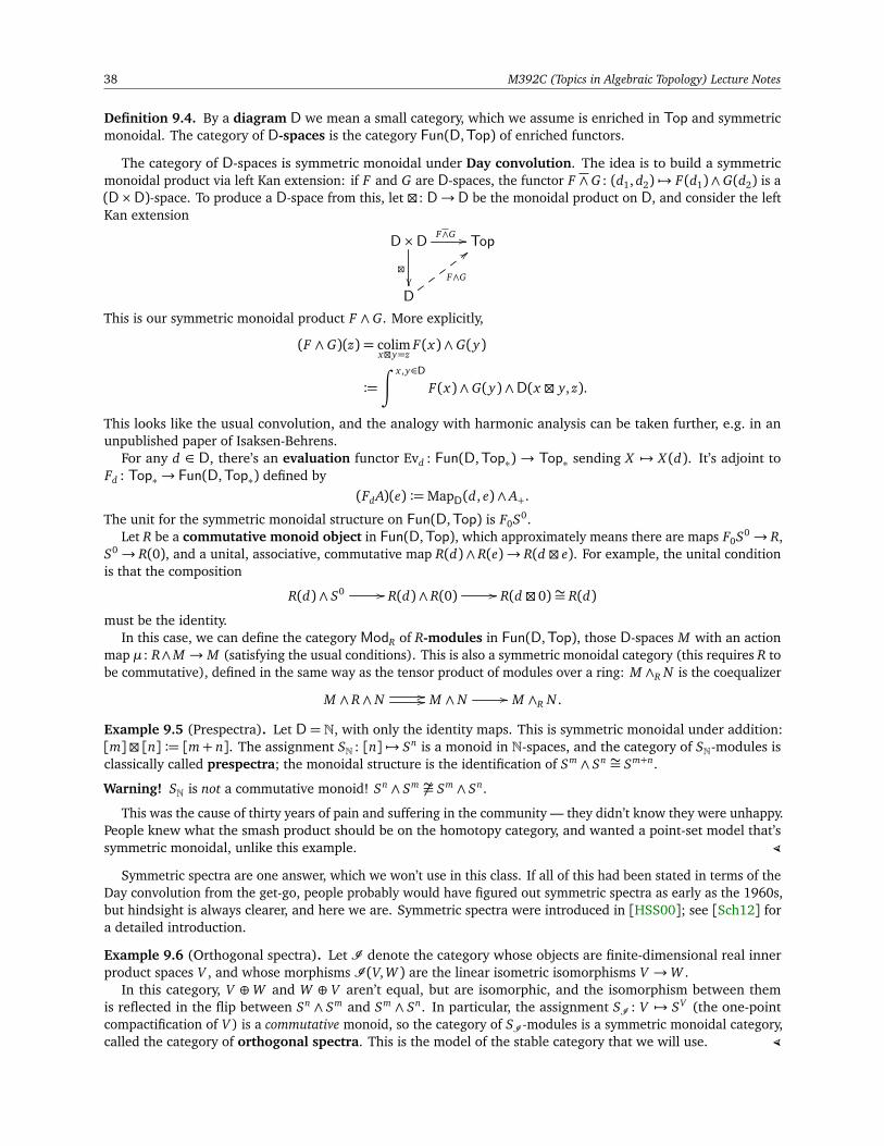
38 M392C (Topics in Algebraic Topology) Lecture Notes
Definition 9.4. By a diagram D we mean a small category, which we assume is enriched in Top and symmetricmonoidal. The category of D-spaces is the category Fun(D,Top) of enriched functors.
The category of D-spaces is symmetric monoidal under Day convolution. The idea is to build a symmetricmonoidal product via left Kan extension: if F and G are D-spaces, the functor F ∧ G : (d1, d2) 7→ F(d1)∧ G(d2) is a(D×D)-space. To produce a D-space from this, let : D→ D be the monoidal product on D, and consider the leftKan extension
D×D F∧G //
Top
D
F∧G
;;
This is our symmetric monoidal product F ∧ G. More explicitly,
(F ∧ G)(z) = colimxy=z
F(x)∧ G(y)
:=
∫ x ,y∈D
F(x)∧ G(y)∧D(x y, z).
This looks like the usual convolution, and the analogy with harmonic analysis can be taken further, e.g. in anunpublished paper of Isaksen-Behrens.
For any d ∈ D, there’s an evaluation functor Evd : Fun(D,Top∗) → Top∗ sending X 7→ X (d). It’s adjoint toFd : Top∗→ Fun(D,Top∗) defined by
(FdA)(e) :=MapD(d, e)∧ A+.
The unit for the symmetric monoidal structure on Fun(D,Top) is F0S0.Let R be a commutative monoid object in Fun(D,Top), which approximately means there are maps F0S0→ R,
S0→ R(0), and a unital, associative, commutative map R(d)∧ R(e)→ R(d e). For example, the unital conditionis that the composition
R(d)∧ S0 // R(d)∧ R(0) // R(d 0)∼= R(d)
must be the identity.In this case, we can define the category ModR of R-modules in Fun(D,Top), those D-spaces M with an action
map µ: R∧M → M (satisfying the usual conditions). This is also a symmetric monoidal category (this requires R tobe commutative), defined in the same way as the tensor product of modules over a ring: M ∧R N is the coequalizer
M ∧ R∧ N // // M ∧ N // M ∧R N .
Example 9.5 (Prespectra). Let D= N, with only the identity maps. This is symmetric monoidal under addition:[m] [n] := [m+ n]. The assignment SN : [n] 7→ Sn is a monoid in N-spaces, and the category of SN-modules isclassically called prespectra; the monoidal structure is the identification of Sm ∧ Sn ∼= Sm+n.
Warning! SN is not a commutative monoid! Sn ∧ Sm 6∼= Sm ∧ Sn.
This was the cause of thirty years of pain and suffering in the community — they didn’t know they were unhappy.People knew what the smash product should be on the homotopy category, and wanted a point-set model that’ssymmetric monoidal, unlike this example. (
Symmetric spectra are one answer, which we won’t use in this class. If all of this had been stated in terms of theDay convolution from the get-go, people probably would have figured out symmetric spectra as early as the 1960s,but hindsight is always clearer, and here we are. Symmetric spectra were introduced in [HSS00]; see [Sch12] fora detailed introduction.
Example 9.6 (Orthogonal spectra). Let I denote the category whose objects are finite-dimensional real innerproduct spaces V , and whose morphisms I (V, W ) are the linear isometric isomorphisms V →W .
In this category, V ⊕W and W ⊕ V aren’t equal, but are isomorphic, and the isomorphism between themis reflected in the flip between Sn ∧ Sm and Sm ∧ Sn. In particular, the assignment SI : V 7→ SV (the one-pointcompactification of V ) is a commutative monoid, so the category of SI -modules is a symmetric monoidal category,called the category of orthogonal spectra. This is the model of the stable category that we will use. (
10 Transfers and the Burnside category: 2/9/17 39
Example 9.7 (W -spaces). Let W be the category of finite CW complexes (with either all maps or cellular maps;it doesn’t really matter). W -spaces are already like spectra, in a sense, in that they’re modules over the identityfunctor i : W ,→ Top. There’s a map ϕ : A→Map(B, A∧B) sending a 7→ (b 7→ a∧ b), so if F is aW -space, we havea sequence of maps
Aϕ // Map(B, A∧ B) // Map(F(B), F(A∧ B)).
Taking its adjoint defines a mapA∧ F(B) −→ F(A∧ B),
so F is a module over i. (
The assignment n 7→ Rn defines a functor N→I , and therefore a functor from prespectra to orthogonal spectra;with the right model structures, this induces an equivalence of their homotopy category. Similarly, the assignmentV 7→ SV defines a functor I →W , hence a functor from orthogonal spectra to W -spaces, and this also will inducea homotopy equivalence.
Definition 9.8. A prespectrum is an Ω-prespectrum if for all n, Xn
∼=→ ΩmXm+n.
Definition 9.9. If X is a prespectrum and q ∈ Z, the qth homotopy group of X is
πq(X ) := colimnπn+qX (n).
A π∗-isomorphism of prespectra is a map that induces an isomorphism on all homotopy groups.
Notice that negative homotopy groups exist, and may be nontrivial.
Remark. This is one approach to defining the stable category, and is not the only one. In [Ada74] (which isan excellent book), Adams uses a more naïve viewpoint of “cells first, maps later” which doesn’t require suchabstraction, but it would be a huge mess to prove that his model is complete or cocomplete. The diagram spectraapproach rigidly separates point-set techniques (easy, but not as useful) from operations on the homotopy category(more useful, but harder), and this separation is often useful. The∞-categorical perspective mashes it all together,which can be confusing, but is the only setting in which you can prove things such as the stable category beinginitial. (
We’ll reintroduce G-actions soon, and this is pretty slick using orthogonal spectra: we can replace I with thecategory of finite-dimensional G-representations with invariant inner products. Orthogonal spectra also have areally nice homotopy theory relative to symmetric spectra (which have other advantages that don’t apply as muchto us).
Lecture 10.
Homotopy theory of spectra: 2/14/17
“But why point-set models?”“Are you serious? I just told you, like, a second ago!” – Zoolander (more or less)
Today, we’re going to discuss the homotopy theory of spectra in the nonequivariant setting. Last time, we discussedD-spaces, where D is a small topological category, and saw that the category of D-spaces is symmetric monoidal.We discussed a few examples:
• Consider D = N with all maps isomorphisms, as in Example 9.5. There’s a noncommutative monoidSN : n 7→ Sn, and the category of SN-modules is called prespectra SpN;38 it’s a monoidal category, but isnot symmetric.
• In Example 9.6, we considered D = I , the category whose objects are real finite-dimensional inner productspaces and whose morphisms are the linear isometric isomorphisms. Here, the monoid SI : V 7→ SV iscommutative, and the category of SI -modules, called orthogonal spectra SpI , is symmetric monoidal.
Those are the main examples for us, but there are others:• When D is the category of finite CW complexes, as in Example 9.7, we obtain W -spaces.• When D is the category of finite, based sets and based maps, as in Example 10.20, we recover Segal’sΓ -spaces.
38There are many different choices of notation for diagram spectra, as seen in [MMSS01] and [MM02], with various fancy decorations.

40 M392C (Topics in Algebraic Topology) Lecture Notes
Because these diagram categories are presheaves on nice categories, they inherit some good properties from Top∗;in particular, they are complete and cocomplete, and limits and colimits may be taken pointwise. This is also truefor categories of modules over monoids in D-spaces, though it requires more work to prove: computing colimits isa bit harder, just like how the free product of groups is more complicated than the direct product. Categories ofrings are not bicomplete, though.
We’ll use prespectra and orthogonal spectra to define Quillen equivalent models for the stable homotopy category.As such, familiar constructions from stable homotopy theory can be constructed as prespectra and orthogonalspectra.
Example 10.1 (Suspension spectra). Let X ∈ Top. The suspension spectrum of X , denoted Σ∞X , is the stablehomotopy type corresponding to the homotopy type of X .
• In prespectra, the suspension spectrum of X is Σ∞X : [n] 7→ Sn ∧ X . The SN-module structure is the dataof the structure maps Sm ∧ (Sn ∧ X )→ Sm+n ∧ X .
• To define an orthogonal spectrum E, one must define for each finite-dimensional real inner product spaceV a pointed space E(V ) with an O(V )-action and for each pair of such inner product spaces V and W , astructure map SV ∧ E(W )→ E(V ⊕W ) that’s O(V )×O(W )-equivariant.
Wanting to do this for every space forces our hand: we have to use the trivial action. The suspensionspectrum of X sends V 7→ SV ∧ X , where the O(V )-action is the usual action in the first componentand the trivial action in the second component. The structure maps SV ∧ SW ∧ X → SV⊕W ∧ X areO(V )×O(W )-equivariant, as desired.
The suspension spectrum of S0 is the sphere spectrum SN or SI . (
Example 10.2 (Eilenberg-Mac Lane spectra). If A is an abelian group, the Eilenberg-Mac Lane spectrum HA isthe spectrum that represents cohomology with coefficients in A. If in addition A is a commutative ring, HA is acommutative monoid in spectra, which defines the ring structure on A-cohomology.
• There is an identification K(A, n)∼=→ ΩK(A, n+ 1); let in : ΣK(A, n) → K(A, n+ 1) be its adjoint. As an
N-space, HA: [n] 7→ K(A, n); the map in makes it into a prespectrum. If A is also a commutative ring,one obtains maps K(A, m)∧ K(A, n)→ K(A, m+ n), and these satisfy the axioms to ensure that HA is acommutative ring spectrum.
• For orthogonal spectra, the construction is more complicated, since we must choose a model for K(A, n)with an On-action on it. In particular, we must assume A is countable. Given an inner product space V ,the A-linearization A[SV ] of SV is, as a set, A tensored with the reduced free abelian group on K (so thebasepoint maps to zero), topologized as the quotient
∞∐
k=0
Ak × (SV )k A[SV ], (a1, . . . , ak, x1, . . . , xk) 7−→k∑
j=1
a j · x j .
This is a model for K(A, dim V ), but has an O(V )-action induced from the O(V )-action on SV . The structuremap SV ∧ A[SW ]→ A[SV⊕W ] sends
(10.3) v ∧
∑
j
a j ·w j
7−→∑
j
a j · (v ∧w j),
and this is O(V ) × O(W )-equivariant, so defines an orthogonal spectrum. If A is a commutative ring,the ring spectrum structure on HA is defined by the multiplication maps µ: A[SV ]∧ A[SW ]→ A[SV⊕W ]sending
µ:
∑
i
ai x i
,
∑
j
b j y j
7−→∑
i, j
(ai b j)(x i ∧ y j),
and the unit maps e : SV → A[SV ] send x 7→ 1 · x . This construction is discussed in more detail in [Sch12,Example I.1.14] and [Sch17, Example V.1.9]. (
Example 10.4 (Thom spectra). TODO (
Definition 10.5. Let f : X → Y be a map of D-spaces (or prespectra or orthogonal spectra).
• f is a level equivalence if for all d ∈D, f (d): X (d)'→ Y (d) is a weak equivalence.
• f is a level fibration if for all d ∈D, f (d) is a fibration.
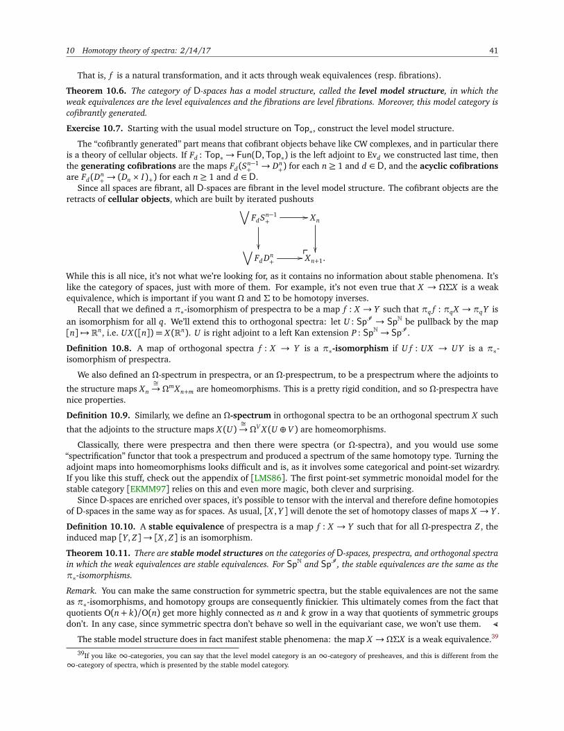
10 Homotopy theory of spectra: 2/14/17 41
That is, f is a natural transformation, and it acts through weak equivalences (resp. fibrations).
Theorem 10.6. The category of D-spaces has a model structure, called the level model structure, in which theweak equivalences are the level equivalences and the fibrations are level fibrations. Moreover, this model category iscofibrantly generated.
Exercise 10.7. Starting with the usual model structure on Top∗, construct the level model structure.
The “cofibrantly generated” part means that cofibrant objects behave like CW complexes, and in particular thereis a theory of cellular objects. If Fd : Top∗→ Fun(D,Top∗) is the left adjoint to Evd we constructed last time, thenthe generating cofibrations are the maps Fd(Sn−1
+ → Dn+) for each n≥ 1 and d ∈ D, and the acyclic cofibrations
are Fd(Dn+→ (Dn × I)+) for each n≥ 1 and d ∈D.
Since all spaces are fibrant, all D-spaces are fibrant in the level model structure. The cofibrant objects are theretracts of cellular objects, which are built by iterated pushouts
∨
FdSn−1+
//
Xn
∨
Fd Dn+
// Xn+1.ð
While this is all nice, it’s not what we’re looking for, as it contains no information about stable phenomena. It’slike the category of spaces, just with more of them. For example, it’s not even true that X → ΩΣX is a weakequivalence, which is important if you want Ω and Σ to be homotopy inverses.
Recall that we defined a π∗-isomorphism of prespectra to be a map f : X → Y such that πq f : πqX → πqY isan isomorphism for all q. We’ll extend this to orthogonal spectra: let U : SpI → SpN be pullback by the map[n] 7→ Rn, i.e. UX ([n]) = X (Rn). U is right adjoint to a left Kan extension P : SpN→ SpI .
Definition 10.8. A map of orthogonal spectra f : X → Y is a π∗-isomorphism if U f : UX → UY is a π∗-isomorphism of prespectra.
We also defined an Ω-spectrum in prespectra, or an Ω-prespectrum, to be a prespectrum where the adjoints to
the structure maps Xn
∼=→ ΩmXn+m are homeomorphisms. This is a pretty rigid condition, and so Ω-prespectra havenice properties.
Definition 10.9. Similarly, we define an Ω-spectrum in orthogonal spectra to be an orthogonal spectrum X such
that the adjoints to the structure maps X (U)∼=→ ΩV X (U ⊕ V ) are homeomorphisms.
Classically, there were prespectra and then there were spectra (or Ω-spectra), and you would use some“spectrification” functor that took a prespectrum and produced a spectrum of the same homotopy type. Turning theadjoint maps into homeomorphisms looks difficult and is, as it involves some categorical and point-set wizardry.If you like this stuff, check out the appendix of [LMS86]. The first point-set symmetric monoidal model for thestable category [EKMM97] relies on this and even more magic, both clever and surprising.
Since D-spaces are enriched over spaces, it’s possible to tensor with the interval and therefore define homotopiesof D-spaces in the same way as for spaces. As usual, [X , Y ] will denote the set of homotopy classes of maps X → Y .
Definition 10.10. A stable equivalence of prespectra is a map f : X → Y such that for all Ω-prespectra Z , theinduced map [Y, Z]→ [X , Z] is an isomorphism.
Theorem 10.11. There are stable model structures on the categories of D-spaces, prespectra, and orthogonal spectrain which the weak equivalences are stable equivalences. For SpN and SpI , the stable equivalences are the same as theπ∗-isomorphisms.
Remark. You can make the same construction for symmetric spectra, but the stable equivalences are not the sameas π∗-isomorphisms, and homotopy groups are consequently finickier. This ultimately comes from the fact thatquotients O(n+ k)/O(n) get more highly connected as n and k grow in a way that quotients of symmetric groupsdon’t. In any case, since symmetric spectra don’t behave so well in the equivariant case, we won’t use them. (
The stable model structure does in fact manifest stable phenomena: the map X → ΩΣX is a weak equivalence.39
39If you like ∞-categories, you can say that the level model category is an ∞-category of presheaves, and this is different from the∞-category of spectra, which is presented by the stable model category.
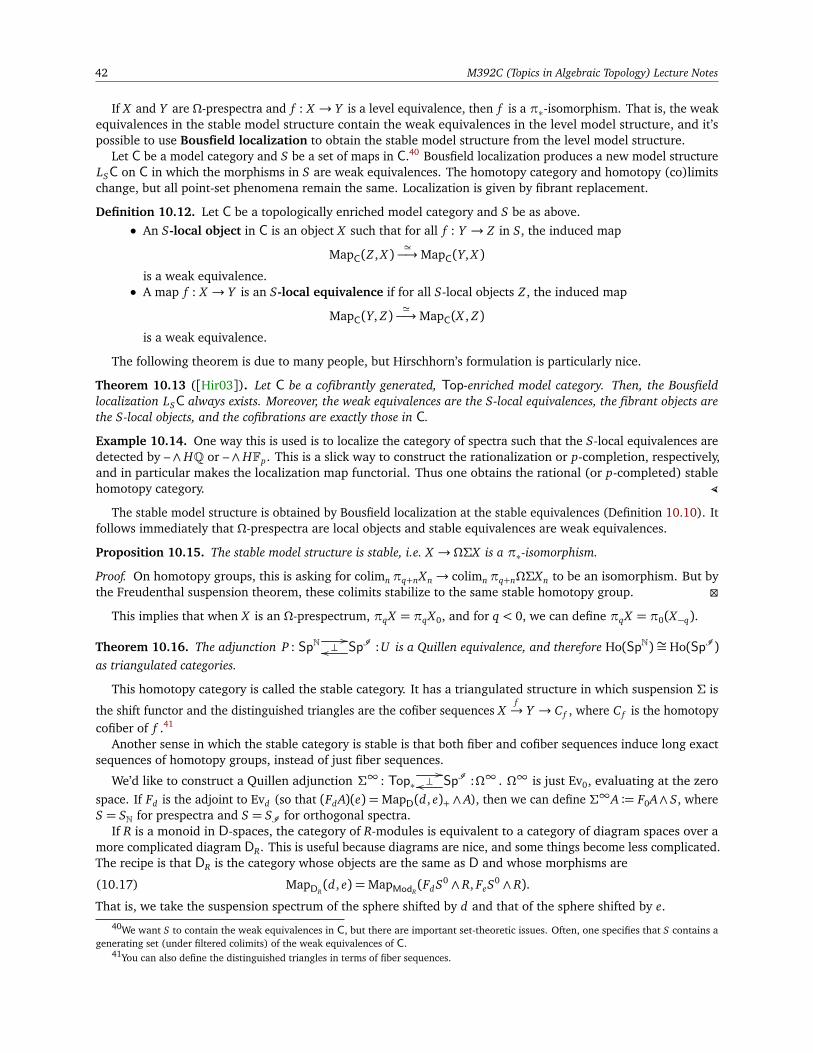
42 M392C (Topics in Algebraic Topology) Lecture Notes
If X and Y are Ω-prespectra and f : X → Y is a level equivalence, then f is a π∗-isomorphism. That is, the weakequivalences in the stable model structure contain the weak equivalences in the level model structure, and it’spossible to use Bousfield localization to obtain the stable model structure from the level model structure.
Let C be a model category and S be a set of maps in C.40 Bousfield localization produces a new model structureLSC on C in which the morphisms in S are weak equivalences. The homotopy category and homotopy (co)limitschange, but all point-set phenomena remain the same. Localization is given by fibrant replacement.
Definition 10.12. Let C be a topologically enriched model category and S be as above.• An S-local object in C is an object X such that for all f : Y → Z in S, the induced map
MapC(Z , X )'−→MapC(Y, X )
is a weak equivalence.• A map f : X → Y is an S-local equivalence if for all S-local objects Z , the induced map
MapC(Y, Z)'−→MapC(X , Z)
is a weak equivalence.
The following theorem is due to many people, but Hirschhorn’s formulation is particularly nice.
Theorem 10.13 ([Hir03]). Let C be a cofibrantly generated, Top-enriched model category. Then, the Bousfieldlocalization LSC always exists. Moreover, the weak equivalences are the S-local equivalences, the fibrant objects arethe S-local objects, and the cofibrations are exactly those in C.
Example 10.14. One way this is used is to localize the category of spectra such that the S-local equivalences aredetected by –∧HQ or –∧HFp. This is a slick way to construct the rationalization or p-completion, respectively,and in particular makes the localization map functorial. Thus one obtains the rational (or p-completed) stablehomotopy category. (
The stable model structure is obtained by Bousfield localization at the stable equivalences (Definition 10.10). Itfollows immediately that Ω-prespectra are local objects and stable equivalences are weak equivalences.
Proposition 10.15. The stable model structure is stable, i.e. X → ΩΣX is a π∗-isomorphism.
Proof. On homotopy groups, this is asking for colimnπq+nXn→ colimnπq+nΩΣXn to be an isomorphism. But bythe Freudenthal suspension theorem, these colimits stabilize to the same stable homotopy group.
This implies that when X is an Ω-prespectrum, πqX = πqX0, and for q < 0, we can define πqX = π0(X−q).
Theorem 10.16. The adjunction P : SpN//
⊥ SpI :Uoo is a Quillen equivalence, and therefore Ho(SpN)∼= Ho(SpI )as triangulated categories.
This homotopy category is called the stable category. It has a triangulated structure in which suspension Σ is
the shift functor and the distinguished triangles are the cofiber sequences Xf→ Y → C f , where C f is the homotopy
cofiber of f .41
Another sense in which the stable category is stable is that both fiber and cofiber sequences induce long exactsequences of homotopy groups, instead of just fiber sequences.
We’d like to construct a Quillen adjunction Σ∞ : Top∗//
⊥ SpI :Ω∞oo . Ω∞ is just Ev0, evaluating at the zerospace. If Fd is the adjoint to Evd (so that (FdA)(e) =MapD(d, e)+ ∧A), then we can define Σ∞A := F0A∧ S, whereS = SN for prespectra and S = SI for orthogonal spectra.
If R is a monoid in D-spaces, the category of R-modules is equivalent to a category of diagram spaces over amore complicated diagram DR. This is useful because diagrams are nice, and some things become less complicated.The recipe is that DR is the category whose objects are the same as D and whose morphisms are
(10.17) MapDR(d, e) =MapModR
(FdS0 ∧ R, FeS0 ∧ R).
That is, we take the suspension spectrum of the sphere shifted by d and that of the sphere shifted by e.40We want S to contain the weak equivalences in C, but there are important set-theoretic issues. Often, one specifies that S contains a
generating set (under filtered colimits) of the weak equivalences of C.41You can also define the distinguished triangles in terms of fiber sequences.
11 Homotopy theory of spectra: 2/14/17 43
Exercise 10.18. Show that for D= N, the structure maps for prespectra come out of (10.17) for R= SN. (This isan adjunction game.) The same is true for orthogonal spectra and SI .
This feels like a Spanier-Whitehead trick, but constructs the right category. In particular, in DR-spaces, Σ∞ isthe left adjoint to evaluating at 0.
It’s possible to bootstrap this to define model categories of ring spectra, i.e. algebras over SI .
Definition 10.19. Let T: SpI → SpI denote the free associative algebra monad, i.e.
TX :=∨
n≥0
X∧n,
so that the category ofT-algebras SpI [T] is the category of associative monoids in SpI . Similarly, let P: SpI → SpI
denote the free commutative algebra monad, so
PX :=∨
n≥0
X∧n/Σn,
where Σn denotes the action of the symmetric group by permutations; thus, the category of P-algebras SpI [P] isthe category of commutative monoids in SpI (i.e. commutative ring spectra).
The stable model structure on SpI induces one on SpI [T], in which the weak equivalences and fibrationsare detected by those in SpI . For SpI [P], the quotient makes things harder: it has a model structure wherethe weak equivalences are positive equivalences (so those which are detected by positive Ω-spectra, i.e. thosewhere X0→ ΩX1 need not be an equivalence). But this still doesn’t behave very well. Namely, if you try to set thetheory up for P to be the same as that for T, then you get that Ω∞Σ∞S0 is a commutative topological monoid.It’s a fact that any commutative topological monoid is a product of Eilenberg-Mac Lane spaces, and that Ω∞Σ∞S0
has nontrivial k-invariants. There’s a short paper by Lewis which addresses this [Lew91], showing that there arefive very reasonable axioms for the stable category that can’t all be true! So people decided to forget about lettingΣ∞ be left adjoint to evaluation at 0, and it’s okay, if not perfect.
Example 10.20 (Γ -spaces). Let D be the category of finite based sets and based maps, e.g. n+ = 0, 1, . . . , n with0 as the basepoint. D-spaces are called Γ -spaces, and agree with Segal’s notion of Γ -spaces, which are defineddifferently. The multiplication comes from the map ψ: 2+→ 1+ sending 1, 2 7→ 1.
Let di : n+→ 1+ send j 7→ δi j (i.e. 1 if i = j, and 0 otherwise). A Γ -space is special if the induced map
X (n+)ϕn−→∏
n
X (1+)
is a weak equivalence; it’s very special if in addition the composition
X (1+)× X (1+) X (2+)'ϕ2oo ψ∗ // X (1+)
induces a commutative monoid structure on π0X (1+).Kan extension defines a functor from D to the category of finite CW complexes, and working withπ∗-equivalences
of these, one obtains a model structure on the category of Γ -spaces. This is Quillen equivalent to the category ofconnective spectra, i.e. those whose negative homotopy groups vanish. (
In the equivariant case, there’s even more structure, and notions of “extra special” Γ -spaces. We’ll spend mostof our time on orthogonal G-spectra, which have nuances of their own, as we’ll see starting next time.
Lecture 11.
The equivariant stable category: 2/16/17
“May your first talk be more peaceful.”Today, we’ll discuss a model for the equivariant stable category, but first we’ll say something about algebras andmonads that went by quickly last time.
Last time, we introduced two monads T and P on SpI , defined as
TX :=∨
k≥0
X∧k PX :=∨
k≥0
X∧k/Σk.
Let’s delve into this a little more.

44 M392C (Topics in Algebraic Topology) Lecture Notes
Definition 11.1. A monad M on a category C is an endofunctor of C which is a monoid in the functor categoryFun(C,C).
That is, there’s a natural transformation µ: M2 → M and a unit, and µ is associative and unital in that therelevant diagrams commute.
There are lots of examples: we’ve already seen that if G is a group, the assignment X → G × X is a monad.More generally, algebraic structures can usually be obtained monadically.
Definition 11.2. Let M be a monad on C. Then, the category C[M] of algebras over M is the category whoseobjects are pairs X ∈ C and structure maps m: MX → X satisfying associativity and unitality for M , and whosemorphisms are the C-morphisms that are compatible with the structure maps.
The associativity diagram, for example, is
M2X m //
µ
MX
m
MX m // X .
We require this to commute.Lots of structures are monadic, e.g. groups are algebras over the free group monad in Set, and similarly for
abelian groups, rings, etc. Monads very generally come from free structures in algebra; they also arise from
adjunctions: an adjunction F : C//
⊥ D :Goo defines a monad GF , with the structure map defined by the unit mapG(FG)F → GF . Many monads arise in this way.
There is always a free-forgetful adjunction F : C//
⊥ C[M] :Uoo , which has to do with the Barr-Beck theorem.Suppose C is a model category. We’d like to lift this to a model structure on C[M]— when does C[M] have amodel structure where the weak equivalences are determined by the forgetful functor U?42 There are two issues.
(1) Since C is complete, so is C[M]: the arrows point the right way. But it’s not always cocomplete.(2) How do we define the model structure?
In order for C[M] to be cocomplete, we’ll use a criterion about preserving certain colimits. Since monads tendto arise from adjunctions, the criterion definitely won’t be true in general! There are seventeen versions of thiscriterion in Mac Lane, but we’ll only need one, following Hopkins and McClure.
Definition 11.3. Let f , g : X ⇒ Y be two maps. A reflexive coequalizer is a coequalizer for f and g togetherwith a simultaneous section s : Y → X for both f and g.
Exercise 11.4. Prove that if M preserves reflexive coequalizers, then C[M] is cocomplete. (This is hard, butworthwhile.)
Proposition 11.5 (Hopkins-McClure). Under very mild hypotheses, T and P preserve reflexive coequalizers.
See [EKMM97] for a proof. SpI satisfies these hypotheses, so we’ve addressed caveat (1).
Theorem 11.6 (Schwede-Shipley [SS00]). Under mild hypotheses, C[M] inherits a model structure from C, wherethe fibrations are detected by U, and the generating cofibrations are M applied to the generating cofibrations of C.
This is a very general theorem; the hard step is constructing a nice enough filtration on pushouts.
Warning! These hypotheses are met for the associative monad T, but are not met by the commutative monad P!This is another formulation of Lewis’ paradox: for commutative ring spectra, you have to change the underlyinghomotopy theory.
Remark. You might be used to thinking of these as the associative and commutative operads. Every operaddetermines a monad, and the operadic algebras become monadic algebras, but for P and T, the explicit form ofthe monad makes it easier to analyze from the monadic viewpoint. (
42This is not how we defined the model structure on G-spaces, but we’ll use it to define model structures on rings and module spectra.

11 The equivariant stable category: 2/16/17 45
Returning to diagram spectra, we’ve been putting a huge emphasis on strict symmetric monoidal structures,rather than just commutativity in the homotopy category. This is useful because it lets you do algebra: if R is a ringin the homotopy category, it’s very hard to control the category of modules, e.g. the cofiber of a map of modulesmay not even be a module, the cyclic bar construction isn’t a simplicial object, etc. Some people have tried to useoperads to fix this, and this is extremely hard: operadic ring spectra are fine, but their modules are not. In a sense,Lurie’s∞-categorical machinery is designed to do this in a more modern way.
A lot of modern homotopy theory has been importing algebraic constructions about rings into homotopy theory,replacing tensor products with smash products. This has been very useful, yet can be hard, and everything is muchmore tractable with a point-set symmetric monoidal structure.
G-spectra. In this context, we must talk about universes, making choices of which orbits G/H are dualizable.This is closely related to choosing representations V such that G/H ,→ V equivariantly.
Definition 11.7. A universe is a countably infinite-dimensional real inner product space with a G-action throughisometries. There is some collection R of irreducible representations such that U contains countably many copiesof each irreducible in R, and R always has all of the trivial representations.43
Sometimes we’ll ask for more structure, such as R being closed under tensor products. The inclusion of thetrivial representation is what makes this a strict generalization of ordinary stable homotopy theory: for example,if U = R∞ with the trivial G-action, the homotopy groups are the nonequivariant homotopy groups.44 Anothercommon choice of U is a complete universe, containing all irreducible representations infinitely often, so allorbits are dualizable.
G-prespectra were defined classically in a manner similar to prespectra. They mix point-set and homotopicaldata, which is a little odd.
Definition 11.8.• A G-prespectrum X is the data of a G-space X (V ) for every finite-dimensional subspace V ⊂ U and
G-maps SW ∧ X (V )→ X (V ⊕W ) for each pair V and W , such that the structure maps are associative.• A G-prespectrum is an Ω-prespectrum if for all V and W , the adjoint to the structure map is a homeo-
morphism: X (V )∼=→ ΩW X (V ⊕W ).
• The homotopy groups of a G-prespectrum are
πHq (X ) := colim
VπH
q ΩV X (V )
πH−q(X ) := colim
V⊃Rm
m>0
πH0 Ω
V−RmX (V ).
Here q ≥ 0, Rm denotes the trivial representation of dimension m, which we specified was in U , andV −Rn denotes the orthogonal complement.
Proposition 11.9. There is a model structure on G-prespectra where the weak equivalences are the stable equivalences(equivalently, π∗-isomorphisms).
The proof is identical to the nonequivariant case. One cool aspect of this is that homotopy groups are determinedby trivial representations, and we’ll see that for orthogonal G-spectra, this is also true at the point-set level. It’snice to not have to carry around the entire universe, just the trivial representations. We’ll use this philosophy inthe proof of Theorem 12.2.
Definition 11.10. The equivariant stable category (structured by U) is the homotopy category of G-prespectra.
This is the category in which we have Poincaré duality for the orbits G/H that embed in U . The functorsΣV := SV ∧ – and ΩV :=Map(SV , –) are inverse equivalences.
Remark. It would be nice to write down some sort of equivariant analogue of a triangulated structure on theequivariant stable category, but trying to get an RO(G)-grading (i.e. shifts by arbitrary representations of G) doesnot work except in ad hoc ways for G = C2. However, you can keep track of the action of the Picard group Pic(SpG)on the equivariant stable category. (
43Ideally, U should not contain other representations. Sometimes people are vague about this, where there may be other representationsand you ignore them, but it’s better to just not have them.
44More explicitly, this is a stabilization of the category of presheaves on BG. Depending on your definitions, this is more or less a tautology— stabilization in∞-categories is defined by taking spectrum objects.
46 M392C (Topics in Algebraic Topology) Lecture Notes
Orthogonal G-spectra. Let’s build a point-set model of the equivariant stable category. Let V and V ′ be finite-dimensional irreducible G-representations (by which we mean finite-dimensional subspaces of U), and let IG(V, V ′)be the linear, G-equivariant isometries.45
Definition 11.11. The complement bundle E(V, V ′) is the subbundle of the product bundle IG(V, V ′) × V ′
consisting of pairs ( f , x) such that x ∈ V ′ − f (V ). Let eIG(V, V ′) denote the Thom space of this bundle.
We’re trying to create spheres: eIG(V, V ′) should topologize SV ′− f (V ). For example, if V ⊂ V ′, this is isomorphicto O(V ′)∧O(V ′−V ) S
V ′−V .Let eIG denote the category whose objects are finite-dimensional subspaces V of U and whose morphisms are
eIG(V, V ′).
Definition 11.12. An orthogonal G-spectrum is a Top-enriched functor eIG → GTop. The category of orthogonalG-spectra is denoted SpG , or SpG
U if the universe needs to be explicit.
For the nonequivariant case, we defined D-spaces and spectra to be modules over a certain monoid in them,and then showed that you could think of them as diagram spaces for a more complicated diagram. Here, we’vedone this all at once — it’s simpler to define eIG than find a module in a simpler category of diagram spaces.
There is a forgetful functor U from SpG to the category of G-prespectra; we define a map f in SpG to be aπ∗-isomorphism if U f is a π∗-isomorphism. SpG is symmetric monoidal under Day convolution, just as before.
Theorem 11.13. SpG has a stable model structure in which the weak equivalences are π∗-isomorphisms, the fibrationsare levelwise fibrations, and the generating cofibrations are
FV
(G/H × Sn−1)+ −→ (G/H × Dn)+
.
Here, FV is adjoint to evaluation at V , as before.Moreover, the smash product is compatible with the model structure. If X is cofibrant, then X ∧ Y computes Tor
X ∧L Y . Another way to say this is that if X is cofibrant, X ∧ – preserves weak equivalences. The proof is wherecofibrantly generated model categories: X ∧ – is a colimit, so it commutes with colimits, and cofibrant objects areretracts of cell complexes, so you can reduce to the case where X is a single cell, which admits a direct proof. Onceagain the stable homotopy category behaves like homological algebra.
Example 11.14. Let X ∈ Sp. Then, “letting G act trivially on X ” defines a G-spectrum also denoted X , such thatfor any n-dimensional G-representation V , X (V ) is, as an On-space, equal to Xn. However, the G-action on X (V )need not be trivial: V and its G-invariant inner product determine a map G→ O(V ), and G acts on X (V ) throughthis map. Since the structure maps respect the G-action, this defines an orthogonal G-spectrum.
One important example is the equivariant sphere spectrum S: S(V ) = SV . It is the unit of SpG . (
Example 11.15 (Suspension spectra). Let X be a based G-space; then, the suspension spectrum of X , denotedΣ∞X , is the G-spectrum whose component on a G-representation V is
Σ∞X (V ) := X ∧ SV .
Given an equivariant map V → W , the structure map Σ∞X (V ) → Σ∞X (W ) is its one-point compactificationsmashed with idX .
In particular, if you give S0 the trivial G-action, Σ∞S0 ∼= S. (
Example 11.16 (Real K-theory). Real K-theory, as discovered by Atiyah [Ati66], is a less generic example.TODO (
We’ll discuss another important example, equivariant Eilenberg-Mac Lane spectra, in Construction 18.7.
Functors on SpG . Let H ⊂ G be a subgroup, so restriction defines a functor iH : SpG → SpH . Just as for G-spaces,iH has a left adjoint G+ ∧H – and a right adjoint FH(G+, –), and these are constructed space-wise.
Proposition 11.17. G+ ∧H – and FH(G+, –) are left (resp. right) Quillen functors.
45Unlike the nonequivariant case, we’re not taking isometric isomorphisms, so maps in IG(V, V ′) must be injective, but may have nontrivialcokernel.
12 The equivariant stable category: 2/16/17 47
Remark. You might worry what universe you end up in after applying iH — naïvely you get the H-representationsthat arise from restriction of G-representations, but you might want all H-representations. The way to address thisis to use a change-of-universe functor, which we’ll mention shortly. This is a good thing to not be sloppy about, but isannoying, and is why people try to get the universe out of the point-set category. In any case, as in group cohomology,induction and coinduction are isomorphic through the Wirthmüller isomorphism (Theorem 12.2). (
One thing that’s nice to do with G-spectra is take fixed points. There are three different ways to do this, namelyhomotopy fixed points, categorical fixed points, and geometric fixed points, and keeping them separate in yourhead is important.
SpG is a closed symmetric monoidal category, meaning it has internal function objects. This is true for D-spacesin general, with internal function objects
FD(X , Y )(n) := F(X , Y (n)).
This is exactly like the mapping complex of two chain complexes: you’re looking at chain maps from X to shifts ofY .
SpG is tensored and cotensored over G-spaces, meaning we can smash G-spectra with G-spaces, and takefunction objects from G-spaces to G-spectra: if A is a G-space, tensoring with A is A+ ∧ – applied levelwise, andcotensoring with A is F(A+, –) applied levelwise.
Definition 11.18.• The homotopy fixed points is the functor X 7→ F(EG+, X )G . (Here, EG+ is a G-space, so we’re using the
cotensor of G-spaces and G-spectra.)• The categorical fixed points is the functor (–)H : X 7→ F(G/H+, X ). As the notation suggests, this is
analogous to (–)H on G-spaces.
Warning! You might hope that (Σ∞A+)H = Σ∞AH+, so that fixed points of spaces lead to fixed points of spectra,
but this is not true. It has a more complicated description called tom Dieck splitting as a wedge of other pieces.
Definition 11.19. The geometric fixed points, denoted ΦH or also X gH , is the unique functor such that
(1) it’s (derived) symmetric monoidal: if X and Y are cofibrant, ΦH(X )∧ΦH(Y )∼=→ ΦH(X ∧ Y ).
(2) ΦH preserves homotopy colimits.(3) ΦHΣ∞X ∼= Σ∞X H .
Of course, uniqueness (up to a contractible space of choices) is a theorem, but it’s true. We’ll also give apreferred construction.
We’ll prove that categorical and geometric fixed points detect weak equivalences.
Theorem 11.20.(1) A map X → Y in SpG is a weak equivalence iff X H → Y H is a weak equivalence for all subgroups H ⊂ G.(2) A map X → Y in SpG is a weak equivalence iff ΦH X → ΦH Y is a weak equivalence for all subgroups H ⊂ G.
This leads one to consider diagrams on categorical or geometric fixed points: because of this perspective, onecan define Tate spectra using this philosophy, and this is particularly useful when applied to S1-spectra. It wasoriginally developed by John Greenlees, and has recently been repopularized and is being mined for applications,such as Nikolaus-Scholze’s description of topological cyclic homology.
We’re going to try to understand the equivariant stable category from a few other perspectives: the Wirthmüllerisomorphism is an analogue of the isomorphism between finite products and coproducts in spectra, and we’ll alsolearn more about tom Dieck splitting. You can also ask how the transfer maps we talked about characterize theequivariant stable category.
Lecture 12.
The Wirthmüller isomorphism: 2/21/17
Today, we’re going to talk about the Wirthmüller isomorphism and tom Dieck splitting. The Wirthmüllerisomorphism is the equivariant analogue of the nonequivariant statement that in the stable homotopy categoryHo(Sp), finite sums and products are equivalent:
(12.1)n∨
i=1
X i
∼=−→n∏
i=1
X i .

48 M392C (Topics in Algebraic Topology) Lecture Notes
This is a backbone of the stable category: among other things, it ensures Ho(Sp) is additive.Tom Dieck splitting is another important structural result about π∗G(Σ
∞X ). When X = S0, this is used tocompute the equivariant stable homotopy groups of the spheres (which is, of course, not completely known). Thiscan be used to recover the Burnside category.
Transfers play a key role in both of these results: it’s somewhat implicit in the Wirthmüller isomorphism, but ispretty explicit for tom Dieck splitting.
The Wirthmüller isomorphism. In this section, we assume G is a finite group. There is a more general statementfor compact Lie groups, but it’s more complicated.
Theorem 12.2 (Wirthmüller isomorphism). Let H be a subgroup of G and X be an object of SpH .46 Then, there is aπ∗-isomorphism G ∧H X
'→ FH(G, X ).
Exercise 12.3. Adapt the proof of (12.1) for nonequivariant spectra to show that the natural map from finitesums to finite products in SpG is also an isomorphism.
However, if you only have (12.1), you’ve described the category of G-spectra structured by a universe with onlytrivial representations!
Applying Theorem 12.2 to X = S0 computes the Spanier-Whitehead duals of orbits.
Corollary 12.4. In the situation of Theorem 12.2, Σ∞(G/H)+ ∼= FH(G, S0)∼= F((G/H)+, S0).
That is, Σ∞(G/H)+ is its own Spanier-Whitehead dual. The slogan is that orbits are self-dual in the equivariantstable category when G is finite.47
Recall that the forgetful map i∗H : SpG → SpH has a left and a right adjoint, respectively G ∧H – and FH(G, –).These spectrum-level constructions are induced by applying the space-level functors levelwise.
Exercise 12.5. Show that these definitions of G ∧H – and FH(G, –) are consistent with the structure maps.
There are three approaches to proving Theorem 12.2.
(1) One is a connectivity argument: show that on the space level, the maps get more and more highlyconnected.
(2) Another approach is to construct an explicit inverse, using a transfer map.(3) One can also set up a Grothendieck six-functor formalism to prove it, which sets up a general theory for
when a lax monoidal functor’s left and right adjoints coincide. See [FHM03, May03, BDS16] for a proofusing this approach; the first and the third papers set up general theory, and the second shows that itapplies to the Wirthmüller map. This makes interesting contact with base-change theory in algebraicgeometry.
Warning! The proof of Theorem 12.2 given in [LMS86] is incorrect, and the fix is nontrivial. It takes approach (2).
We’ll use a connectivity argument, which will introduce some tools we’ll find useful later.
Proof of Theorem 12.2 (X connected). Though we assume X is connected, the same proof can be adapted when Xis bounded-below. The theorem is true for general X , but this proof may not work in that case.
Let X ∈ HTop∗. Then, there’s a map θ : G ∧H X → FH(G, X ) defined by
θ (g1, x)(g2) =
¨
g2 g1 x , g2 g1 ∈ H∗, otherwise.
Exercise 12.6. Show that θ is a G-map.
θ induces a map θ : G∧H X → FH(G, X ) in SpG . We’ll show that it’s an equivalence by computing the connectivityof θ .
Let K ⊆ G, ρ be the regular representation of G, and m ∈ N. Then, we’ll compute the connectivity of
θm,K : (G ∧H ΣmρX )K −→ (GH(G,ΣmρX ))K .
46Here, we’re implicitly using the complete universe U to define SpG and SpH .47When G is a compact Lie group, there’s a degree shift arising from the tangent representation of G on the Lie algebra of H. TODO:
double-check this.
12 The Wirthmüller isomorphism: 2/21/17 49
When G is finite, the sequence (ρ, 2ρ, 3ρ, . . . ) is cofinal (i.e. the colimits are the same) in the filtered diagram offinite-dimensional representations of the complete universe U . Thus, to understand colimV⊂U Ω
VΣV X , it sufficesto understand what happens when V = mρ.
Exercise 12.7. The reason this is true is that when G is finite, the regular representation ρ contains a copy ofevery irreducible as a summand. Prove this by doing a character computation.
We’ll show the connectivity of θm,K is increasing in m, which means that πK∗ θ : πK
∗ (G ∧H X )→ πK∗ (FH(G, X )) is
an isomorphism.The calculation itself will use the K , H double coset decomposition of G to identify the K-fixed points as a sum
and as a product, and we understand the connectivity of both of these from nonequivariant homotopy theory.Let S ⊂ G be a set of representatives for the double coset partition of G, i.e. under the K ×H-action (k, h) · g =
k−1 gh. Then,
(12.8) (G ∧H Z)K =
∐
g∈S
(K gH)+ ∧H Z
!K
.
Either g−1K g ⊆ H or it isn’t.
• If g−1K g ⊆ H, then the action is only in Z , so ((K gH)+ ∧H Z)K = Z g−1K g .• If g−1K g 6⊆ H, then the action is free, so ((K gH)+ ∧H Z)K = ∗.
In particular (12.8) simplifies to
(G ∧H Z)K ∼=∨
g∈Sg−1K g⊆H
Z g−1K g .
Next we look at (FH(G, Z))K . If S is a set of representatives of the double cosets, so is S−1 := g−1 | g ∈ S, so wecan decompose
(FH(G, Z))K ∼=
FH
∐
g∈S
K g−1H, Z
!!K
∼=∏
g∈S
FH(K g−1H, Z)K
∼=∏
g∈S
Z (gK g−1)∩H ∼=∏
g∈S
Z (g−1K g)∩H .
This identification sends f 7→ f (g); the last equivalence is by using S−1 as the set of representatives instead of S.In particular, the space-level Wirthmüller isomorphism may be written
(12.9)∨
g∈Sg−1K g⊆H
Z g−1K g∼=−→∏
g∈S
Z (g−1K g)∩H .
This is nice-looking, but the indexing sets are slightly different. To overcome this, we’ll factor (12.9) as∨
g∈Sg−1K g⊆H
Z g−1K g ϕ1 //∏
g∈Sg−1K g⊆H
Z (g−1K g)∩H ϕ2 //
∏
g∈S
Z (g−1K g)∩H ,
where ϕ1 is the natural map from the sum to the product and ϕ2 is inclusion. Then, we will estimate theconnectivity of ϕ1 and ϕ2 separately in the case when Z = ΣmρX . Namely, we’d like to show that they’re both(m[G : K] +O(1))-connected.
First, what are the fixed points in (Smρ)g−1K g? This is a sphere whose dimension has been shrunk by K, so
smashing with it produces something m[G : K]-connected. Then, the usual argument about turning sums intoproducts says that ϕ1 is about 2m[G : K]-connected.
For ϕ2, what’s the connectivity of the missing factors in the domain? In this case, the connectivity is aboutm[G : K].

50 M392C (Topics in Algebraic Topology) Lecture Notes
Thus, the connectivity of θm,K is m([G, K] +O(1)),48 so the spectrum-level map θ is a πK∗ -isomorphism. More
precisely, the cofiber of θ : G ∧H X → FH(G, X ) has trivial πK∗ , and there’s a little bit to do here to check this.
Remark. Let’s see how this connects to the transfer. Let V be a G-representation such that there’s an embeddingG/H ,→ V . Then, we obtain an H-map G ∧H SV → SV that takes points in G \H to the basepoint. The adjoint ofthis map is the G-map G ∧H SV → FH(G, SV ).
On the other hand, we have a Pontrjagin-Thom map SV → G ∧H SV induced as follows: G/H ,→ V induces amap G ∧H D(V )→ V , and therefore a map SV → G ∧H D(V )/(G ∧H S(V ))∼= G ∧H SV . The observation is that thecomposition SV → G ∧H SV → SV is the identity (you can and should think about this: it’s possible to write downan explicit homotopy inverse). This motivates the slogan that “the Wirthmüller isomorphism is the inverse of thetransfer map,” which we’ll say more about later. (
Tom Dieck splitting. Tom Dieck splitting is a decomposition of the fixed points of a suspension G-spectrum, eitherof the statements
(Σ∞X )G ∼=∨
(H)⊆G
EWH+ ∧WH X H(12.10a)
π∗(Σ∞X )G ∼=
⊕
(H)⊆G
πWH∗
Σ∞EWH+ ∧WH X H
.(12.10b)
By (H) ⊆ G, we mean indexing over the conjugacy classes of subgroups of G. Here WH = NH/H as usual; if H Å G,then this is G/H. Tom Dieck splitting looks complicated; you might have hoped that Σ∞ and (–)G commute, butthey don’t, and this is how they don’t. But when X = S0, this tells you a decomposition of πG
∗ (S).We have a cofiber sequence, called the isotropy separation sequence,
EG+ //S0 //ÝEG,
which induces for any spectrum X a cofiber sequence
(12.11) (EG+ ∧ X )G //X G //(ÝEG ∧ X )G .
Take X = S= Σ∞S0, giving
(Σ∞EG+)G //SG //(Σ∞ÝEG)G .
There are three key observations; one is easy, one is harder, and the one was a major structural theorem.
• When X is a suspension spectrum, (12.11) splits.• The Adams isomorphism tells us the cofiber: (Σ∞EG+)G ' Σ∞BG+.• The last term is (ÝEG ∧ X )G ∼= ΦGX .
Tom Dieck proved tom Dieck splitting by inducting over isotropy sequences, adding one conjugacy class at a time.This is one of the two major methods of induction in equivariant homotopy theory (the other being induction overcells), and was a key step in the resolution of the Kervaire invariant 1 problem [HHR16a].
Lecture 13.
Tom Dieck splitting: 2/23/17
Today, we’ll again assume that G is a finite group. Some of today’s content extends to compact Lie groups, butit’s more complicated.
Last time, we saw the Wirthmüller isomorphism (Theorem 12.2), which we said can be used to create thetransfer maps. One consequence is Corollary 12.4, that orbits are self-dual under Spanier-Whitehead duality:D(G/H+) = Σ∞G/H+. You can use this to write down the transfer map: given subgroups K ⊆ H ⊆ G, we have the“right-way” map G/H → G/K, and therefore a map Σ∞(G/K+) ∼= D(G/K+)→ D(G/H+) ∼= Σ∞(G/H+). By theWirthmüller isomorphism, this is the same as a map F(G/K+, S)→ F(G/H+, S), which is exactly the transfer map!
This is a little circular; if you look carefully into the proof of Theorem 12.2, the transfer map is already there.But the point is more philosophical: the existence of transfers is the same thing as the Wirthmüller isomorphism.
Remark. Transfer maps can be studied in more generality, e.g. in the context of equivariant vector bundles onhomogeneous spaces. Rothenberg wrote some stuff, but [LMS86] is probably the best source. (
48TODO: I want to run through the connectivity carefully and ensure I made no typos.

13 Tom Dieck splitting: 2/23/17 51
Today we’ll talk about tom Dieck splitting. There are several closely related versions of the statement, thoughgoing between them requires a deep result called the Adams isomorphism. We’ll return to that point later.49
Anyways, we’ll prove the version in (12.10b).When X = S0, this “computes” the equivariant stable homotopy groups of the spheres, and one consequence is
that
(13.1) πG0 (Σ
∞S0)∼=⊕
(H)⊆G
Z,
i.e. it’s free on the conjugacy classes of subgroups of G.As a consequence of the proof of (12.10b), the generators are given by the Euler characteristics S→ Σ∞G/H+→
S.50 This lets us identify homotopy classes of stable maps G/H1→ G/H2; since we defined the Burnside categoryto be the full subcategory of SpG on Σ∞G/H+, this amounts to the computation of π0BG .
Define an abelian group A whose generators are diagrams of the form
(13.2) G/H1 G/Kθ1oo θ2 //G/H2,
and for which two diagrams G/H1 ← G/K → G/H2 and G/H1 ← G/K ′ → G/H2 are equivalent if there is anisomorphism f : G/K → G/K ′ such that the following diagram commutes.
G/K
o f
θ2
((θ1
vvG/H1 G/H2.
G/K ′θ ′1
hh
θ ′2
66
The point is that there’s an isomorphism ψ: A∼=→ πH1
0 (Σ+G/H2), the group of stable maps G/H1→ G/H2. We’llcalculate these maps in the algebraic Burnside category π0(BG). The isomorphism ψ takes a diagram of theform (13.2) to the composite Σ∞+ G/H1→ Σ∞+ G/K → Σ∞+ G/H2, where the first map is the transfer for θ1 and thesecond is Σ∞θ2.
Exercise 13.3. Show that ψ is an isomorphism.
This is really nice: we have a nice combinatorial description of the stable maps coming from the structure of G.But what’s the composition?
The above is more or less true for G a compact Lie group. But what follows really requires G to be finite.It seems natural to play double coset games here, but this quickly turns into a notational mess. But if you know
about spans, there’s only one thing it should be, which is the pullback:
G/K ×G/H2G/K ′
G/K ′
G/H3.
G/K
G/H2
G/H1
This is true, and we’ll give a real proof later. The upshot is really cool: we have a complete combinatorial descriptionof the algebraic Burnside category, including composition. This leads one to Mackey functors: equivariant stablehomotopy theory is controlled by a pair of functors out of the orbit category, one covariant and one contravariant,and Mackey functors are nice examples of these.
Remark. We’ve been tacitly assuming a complete G-universe for this, but what if you’d prefer to leave out certainsuspensions ΣV ? In the case of an incomplete G-universe U , you only consider the orbits G/H ,→ U , and build theincomplete Burnside category and incomplete Mackey functors in this way. (
Now let’s prove tom Dieck splitting.
49TODO: I missed one version of the splitting.50TODO: I didn’t understand this.

52 M392C (Topics in Algebraic Topology) Lecture Notes
Proof of (12.10b). We’ll approach this inductively and look a single summand at a time, producing a map
(13.4) πWH∗
Σ∞EWH+ ∧ X H
−→ πG∗ (Σ
∞X ).
Recall that WH = NH/H, so we can define a sequence
(13.5) πWH∗
Σ∞EWH+ ∧ X H θ1 // πNH
∗
Σ∞EWH+ ∧ X H θ2 // πNH
∗ (Σ∞EWH+ ∧ X ),
where θ1 is induced by restriction πWH∗ → π
NH∗ , and θ2 is induced from the inclusion X H ,→ X . The Wirthmüller
isomorphism induces an isomorphism on homotopy groups πH∗ (X )
∼=→ πG∗ (G ∧H X ) (by an adjunction game), so we
can extend (13.5) with maps
πNH∗ (Σ
∞EWH+ ∧ X )θ3
∼=// πG∗ (G ∧NH Σ
∞EWH+ ∧ X )θ4 // πG
∗ (Σ∞X ).
Here, θ4 is the adjoint of the NH-map Σ∞EWH+ ∧ X → Σ∞X that crushes EWH→ ∗. Thus, our goal is to provethat θ2 θ1 and θ4 are isomorphisms.
Recall that a Z-graded homology theory on G-spaces is a collection of functors Eq : GTop→ Ab for q ∈ Z thatare homotopy invariant and such that
Eq
∨
k
Xk
∼=⊕
k
Eq(Xk),
and a map f : X → Y induces a long exact sequence
(13.6) · · · // Eq(X ) // Eq(Y ) // Eq(C f ) δ // Eq−1(X ) // · · ·
The key observation is that both sides of (12.10b) specify Z-graded homology theories.
Definition 13.7. An X ∈ GTop is concentrated at a conjugacy class H if for all K not in the conjugacy class ofH in G, X K is contractible.
Theorem 13.8. Let h: Eq → Eq be a natural transformation of Z-graded homology theories. If h is an isomorphismon all X concentrated at a conjugacy class, then h is an isomorphism.51
This leads to a very innovative proof, invented by tom Dieck, whose pedagogical importance is just as significantas the theorem statement: we’ll set up a sequence of families of subgroups of G
e=F0 ⊆F1 ⊆F2 ⊆ · · · ⊆ Fn = H ⊆ G
such that Fi is built from Fi−1 by adding a conjugacy class not already present. Then, we can induct on i, andsince G is finite, this must terminate. This is one of the key techniques of induction in equivariant homotopy theory,along with cellular induction.
Proof of Theorem 13.8. Let’s induct: suppose that Fi =Fi−1 ∪ (K) for some K ⊆ G, and consider any G-space X .There is a natural map f : X ∧ EFi−1→ X ∧ EFi , and its cofiber C( f ) is concentrated at K!
Suppose that Eq(X ∧ EFi−1)∼=→ Eq(X ∧ EFi−1). By hypothesis, Eq(C( f ))
∼=→ Eq(C( f )), since C( f ) is concentratedat K. Now, by the long exact sequence (13.6) and the five lemma, the map Eq(X ∧ EFi)→ Eq(X ∧ EFi) is anisomorphism.
Now, to prove tom Dieck splitting, it suffices to show that the map we defined (the direct sum of (13.4) over allconjugacy classes) is an isomorphism when X is concentrated at a single conjugacy class (H).
First, we’ll show that if X is concentrated at (H) and K 6∈ (H), then (13.4) is trivial for K. Let’s considerΣ∞EWK+ ∧ X K . Look at the space SV ∧ EWK+ ∧ X K , and let’s consider its L-fixed points for L ⊆ K. If L = e,then (X K)L is contractible, and otherwise, (EWK+)L is contractible, so the smash product is always contractible.We conclude that Σ∞EWK+ ∧ X K is contractible, and therefore that
πWK∗
Σ∞EWK+ ∧ X K
= 0.
Now we’ve reduced to showing that (13.4) is an isomorphism when X is concentrated at H, i.e. that (13.5) is anisomorphism (its components aren’t) and that θ4 is an isomorphism.
51The analogue of this theorem for Z-graded cohomology theories is also true.
14 Tom Dieck splitting: 2/23/17 53
Let’s first tackle θ4.52 This uses an important piece of technology: suppose X and Y are G-spaces and H ⊆ G isnormal. Then, there is a restriction map
ρH : MapG(X , Y ) −→MapG/H(X H , Y H).
This map appears in an essential way in the definition of topological cyclic homology.53
Lemma 13.9. Suppose Y is concentrated at (H); then, the restriction map ρH : MapG(X , Y )→MapG/H(X H , Y H) isan acyclic fibration.
We’ll prove this next time with cellular induction; in any case, we only need that ρH is a weak equivalence.Anyways, we want to show that (13.5) is an isomorphism, so we’ll use the restriction map to define an inverse
πNH∗ (Σ
∞EWH+ ∧ X )→ πWH∗ (Σ
∞EWH+ ∧ X H). That is, consider
[Sn+mρNH , SmρNH ∧ EWH+ ∧ X ]
and take the H-fixed points on both sides; Lemma 13.9 ensures this is an isomorphism.
As this is a statement about stable homotopy groups, it’s desirable to have a spectrum-level equivalence whichreduces to this isomorphism; the statement is (12.10a), but the proof is different.
Lecture 14.
Question-and-answer session II: 2/24/17
Question 14.1. Are orthogonal spectra the same as diagram G-spectra indexed on all finite-dimensional represen-tations of G? If so, what are the advantages of working with only orthogonal representations? Is orthogonalityneeded to make sense of Ω-spectra?
Much of it is that the representations in question often come with a natural inner product. Also, it’s useful totake orthogonal complements sometimes. Nonetheless, it’s probably not strictly necessary.
Question 14.2. What conditions need to be put on a diagram category D such that D-spectra are Quillen equivalentto orthogonal spectra?
It’s hard to be precise about this, but one thing that’s common to all of them is an embedding of N into Dproducing an adjunction between the forgetful functor and the prolongation functor. We used the forgetful functorto define the homotopy groups. So if you can embed N into it, it’s probably OK, but it’s doubtful that a complete,explicit classification exists. Γ -spaces are kind of strange, though.
Question 14.3. There are geometric fixed-points, homotopy fixed-points, and categorical fixed-points. What’s theintuition for what these three constructions are doing?
Recall that the categorical fixed points are (–)H = F(Σ+G/H, –), which tom Dieck splitting tells us is complicatedand hard to compute in general. The homotopy fixed points F(EG+, –)G are more computable: there’s a spectralsequence arising from the filtration of BG. Geometric fixed points ΦH X , which satisfy the property ΦHΣ∞X ∼=Σ∞X H (and are uniquely characterized by this, being strong symmetric monoidal, and preserving homotopycolimits), have nice properties.
You can also analyze them in terms of what they do to S−V , i.e. the Spanier-Whitehead dual of SV : geometricfixed points will send it to S−V H
, whereas categorical fixed points will look more like a tom Dieck splitting.It’s possible to write every spectrum as a colimit of suspension spectra, and this “canonical presentation” is a
good way to dissect the differences between these fixed points. We might talk more about this later.Both the categorical and geometric fixed points detect weak equivalences, so you could use, e.g. the geometric
fixed points to define homotopy groups.Tate spectra fit into this story: the Tate spectrum X tC of X fit into a homotopy pullback diagram (27.5) where
the other three corners are the three kinds of fixed points. This looks like an arithmetic square, and this analogycan be made precise.
Question 14.4. Is there a similar story for coinvariants? Are there categorical, homotopical, and geometriccoinvariants?
52TODO: I got confused and should fix this.53The new construction of TC by Nikolaus-Scholze manages to avoid this in a way that is considerably more natural.

54 M392C (Topics in Algebraic Topology) Lecture Notes
Not really, so far: Lewis and May remark that the construction you would write down is hard to control, andhard to derive. It’s possible that new work on the foundations of equivariant homotopy theory could enable abetter answer, but nothing’s been done right now.
Question 14.5. Are there notions of naïve and genuine G-spaces? (This question was asked in the homotopytheory chatroom on MathOverflow.)
The terminology is less common than that of naïve and genuine G-spectra; in some sense, it’s a little weird tobe using terms like “genuine” and “naïve” in the first place to describe mathematical objects. In any case, by agenuine G-space, we mean a functor out of the orbit category, but a naïve G-space would be a functor out of thecategory containing just G/e, so capturing only the theory of spaces over BG.
On the subject of mathematical literature, the HULK smash product [Man12] is possibly the best mathematicaljoke of all time.
Question 14.6. You’ve said that Hill-Hopkins-Ravenel [HHR16a] has significantly affected the direction of equi-variant stable homotopy theory. Can you elaborate on this?
There’s been some interest in S1-equivariant methods, but a big piece has been a focus on computations, nowthat some computations look possible. The use of trace methods is also exciting. There’s some work on relatingequivariant homotopy theory to motivic homotopy theory, which looks exciting.
Another generalization is to global homotopy theory; Stefan Schwede has a program for setting this up. One ofthe eventual payoffs will be an equivariant TMF, which Lurie has sketched a construction of.
Question 14.7. Has the Tannakian formalism been applied to this context? Maybe instead of a universe ofrepresentations, it would be easier to take a category.
This hasn’t really been considered; it might be interesting, and it might be hard to work with.
Question 14.8. If you like to think of spectra as infinite loop spaces, what changes in the equivariant case?
For G a finite group, everything is the same: you can use Γ -G-spaces or ΓG-spaces (which are different notions forthe same thing by Theorem 25.1); you can use functors from Γ to G-spaces, and a few other ones. Then, loop spacescome from a E∞-operad action; for technical reasons you may need to assume there are trivial representations inthe universe.
In the case of compact Lie groups, nobody really knows how to set up the theory of infinite loop spaces. Inparticular, being an E∞-G-space is not the same as being the zero space of a G-spectrum.
One way to think about this is that on the space level, the E∞ operad controls the transfers. The issue is thatwe only know how to handle finite-index transfers and norms; maybe you should put them in freely, but you getweird obstructions. There’s lots of interesting questions to be asked here, but they are hard and likely not worthyour time.
Question 14.9. What is a cyclotomic spectrum?
Fix a prime p; a p-cyclotomic spectrum is an S1-spectrum X together with data of an equivalence with itsCp-geometric fixed points as S1-spectra.
Recall that the loop space of X is LX :=Map(S1, X ). Its suspension spectrum is an example of a cyclotomicspectrum: there is an identification ΦCp(Σ∞+ LX )∼= Σ∞+ (LX )Cp ∼= Σ∞+ LX .
If X is an S1-spectrum, we can take X Cpn ∼= (X Cp)Cpn−1 → (ΦCp X )Cpn−1 → X Cpn−1 , and the homotopy limit of thesemaps is topological cyclic homology.
Question 14.10. What are cyclonic spectra?
It’s not a standard term, and the professor didn’t remember off the top of his head.
Question 14.11. Is there an analogue of the regular representation in stable homotopy theory?
The answer is, not really. This relates to the complicated structure of tom Dieck splitting — even in the case forcompact Lie groups, where the proofs we gave don’t completely generalize, there are versions of the Wirthmüllerisomorphism and tom Dieck splitting that have shifts by the tangent representation at the identity coset of G/H.This shift pops up again and again.
Question 14.12. What is currently happening in EDAG? What roadblocks are currently in the way?

15 Question-and-answer session II: 2/24/17 55
When you look at TMF, especially with level structure, it really looks like there should be some underlyingequivariant spectrum, and it would be nice to have a way to make this explicit.
There are issues with localization behaving poorly, and∞-operads were introduced to make things behavebetter. It’s also conceptually interesting and cool how the action of an∞-operad controls what transfers it has,and suspension converts the transfers into norms, and you get a ring spectrum: it’s a nice conceptual picture thatexplains what’s going on.
Question 14.13. What applications have there been besides [HHR16a] and trace methods?
Both of those are good applications. A lot of the interesting work in chromatic homotopy theory regarding,e.g. homotopy fixed points of subgroups of the Morava stabilizer group, uses G-actions. Stable representationtheory of finite groups also uses this material. Goodwillie calculus also uses equivariant methods: Nick Kuhnproved in [Kuh04a] that the vanishing of extensions in the Taylor tower is equivalent to the vanishing of the Tatespectrum.
There’s an analogue of Goodwillie calculus for the equivariant setting, an “equivariant calculus;” since calculusis about passage from the unstable to the stable category, the equivariant stable category plays the analogous rolein equivariant calculus.
Completion with respect to the (Σ∞,Ω∞)-adjunction is important in calculus, in terms of a simplicial resolution,and it’s a little weird that you get the same answer if you complete with the correct or the trivial choice.54
Question 14.14. In a vague sense, the classification of groups splits into two parts: find the simple pieces (finitesimple groups) and figure out how to put then together (which is also hard). Algebraic K-theory throws out thesecond part: is there any way to understand the category of finitely-presented groups in this way?
Jeff Smith used a similar method in a different context, but it hasn’t been extremely fruitful. People haven’tlooked into the K-theory of finitely presented groups, and it might be interesting.
Question 14.15. What did you mean by the generators of πG0 (S
0) being Euler characteristics as a consequence oftom Dieck splitting?
πG0 (S
0) is equivariant homotopy classes of maps from S0 to itself. This is free on conjugacy classes — well, whatmaps generate? The answer is the composites of the maps S→ Σ∞G/H+ and the crush map back to S: these areEuler characteristics, in that these are equivariant analogues of the maps whose degrees give Euler characteristicsin the nonequivariant case?
Question 14.16. How much more bananas is the equivariant sphere than the sphere?
It’s way more complicated: it has ΩV SV in it for all V , and the decomposition is not nice. Maybe for specificgroups you can say something nice.
Question 14.17. Knowledge of facts about the sphere spectrum encodes information interesting in other fields.Does knowledge about the equivariant sphere spectrum tell us anything more than the equivariant generalizationsof those results?
Presently, no such applications are known.
Question 14.18. Under certain conditions, you can detect the homotopy groups of a spectrum by looking at the 0level. Can you do this for G-spectra by looking at the regular representation?
Better, in fact: in the case of an Ω-G-spectrum, you can compute the homotopy groups at the trivial representa-tion.
Question 14.19. What is the status of Grothendieck’s approach to homotopy theory?
That’s a good question; it’s not so clear. People like derivators, because they’re 2-categorical and thereforeeasier to deal with, but they might go away once the higher-categorical foundations get standardized.
Question 14.20. In equivariant homotopy theory, there are multiple kinds of suspension functor. How does onethen conclude that cofibers are the same as fibers up to some shift, if there are multiple choices of shift to make?
This is a great exercise for you to work out.54TODO: better word than “choice.”

56 M392C (Topics in Algebraic Topology) Lecture Notes
Lecture 15.
The Burnside category and Mackey functors: 2/28/17
Today, we’re going to finish the proof of tom Dieck splitting, at least on the level of homotopy groups (12.10b).We’ll defer the spectrum-level theorem (12.10a) to later.
We’ve reduced to showing that the composite
πWH∗ (Σ
∞EWH+ ∧ X H) //
θ1
**
πNH∗ (Σ
∞EWH+ ∧ X H)
πNH∗ (Σ
∞EWH+ ∧ X )∼= // πG
∗ (G ∧H Σ∞EWH+ ∧ X )
θ2 // πG∗ (X )
is an isomorphism when X is concentrated at the single conjugacy class (H) for G. The composite of the firsttwo maps is denoted θ1. We did this by showing that the two sides of the tom Dieck isomorphism are Z-gradedhomology theories, and therefore are determined by their values on spaces concentrated at single conjugacy classes.We’ll show separately that θ1 and θ2 are isomorphisms.
First let’s look at θ2, by looking at the spaces of the suspension spectrum for
G ∧NH
EWH+ ∧ X ∧ SVK
.
Fixed points do not commute with suspension on the spectrum level (after all, this is the content of tom Diecksplitting), but they do commute with the smash product for spaces, so this is also
(G ∧H EWH+)K ∧ X K ∧ SV K
.
If K 6∈ (H), then X K ' ∗, since X is concentrated at (H). If K ∈ (H), then (EWH+)K ' ∗, so either way what weobtain is an isomorphism for θ K
2 .For θ1, we needed to prove Lemma 13.9, that if H Å G and Y is concentrated at (H), then the restriction map
MapG(X , Y )→MapG/H(X H , Y H) is an isomorphism.
Proof of Lemma 13.9. The proof will proceed by cellular induction. Consider attaching a cell to a G-space Z toform a space Z , which is expressed by the pushout
G/K+ ∧ Sn−1 //
Z
G/K+ ∧ Dn // Z .ð
If we apply MapG(–, Y ) to this diagram, it becomes a pullback
MapG(G/K+ ∧ Sn−1, Y ) MapG(Z , Y )oo
MapG(G/K+ ∧ Dn, Y )
ψ1
OO
MapG(Z , Y ).oo
ψ2
OO
Since MapG(G/K+ ∧ Sn−1, Y )'Map(Sn−1, Y K), then ψ1 is trivial, so ψ2 is an isomorphism.Let
X0 := x ∈ X | Gx 6⊆ H ⊆ X .
Then, X \ (X0 ∪ X H) is built by attaching cells G/K+ ∧ Dn with K 6∈ (H).The cell attachment computation we just made tells us that it suffices to understand X0 ∪ X H , for which we use
a Mayer-Vietoris argument associated to the pullback
X0 ∪ X H X Hφ1oo
X0
OO
X0 ∩ X Hφ2oo
OO

15 The Burnside category and Mackey functors: 2/28/17 57
We again apply MapG(–, Y ); this time, the same argument shows that φ∗2 is an isomorphism. Now the map wewant factors as
MapG(X , Y ) // MapG(X0 ∪ X , Y ) // MapG(X H , Y ) // MapG/H(X H , Y H).
The last map comes from the adjunction, and in particular is a known weak equivalence. And by induction, thefirst two maps are weak equivalences.
We’ll use Lemma 13.9 to check that the map
πWH∗ (Σ
∞EWH+ ∧ X H)θ1−→ πNH
∗ (Σ∞EWH+ ∧ X )
is an isomorphism, by providing a map in the other direction. Specifically, this is a map of homotopy classes
[Sn+mρ,ΣmρEWH+ ∧ X ]θ1−→ [Sn+mρ,ΣmρEWH+ ∧ X ].
We’ve abused notation a bit here: on the left, ρ is the regular representation for NH, and on the right, it’s theregular representation for WH. Lemma 13.9 implies that the map going the other way is an isomorphism when Xis concentrated at (H):
[Sn+mρ, Smρ ∧ EWH+ ∧ X ]∼=−→ [Sn+mρH
, SmρH∧ EWH+ ∧ X H].
This is what we reduced the problem to, so we have completed the proof of tom Dieck splitting for π∗G(Σ∞X ) on
the level of homotopy groups.
The Burnside category. Let C be a small category with finite limits and finite coproducts. In C, consider thediagram
Xϕ1 //
Y
Z
ϕ2oo
X ′ // X ′ q Z ′ Z ′.oo
Both of these squares are pullbacks iff Y ∼= X q Z with ϕ1 and ϕ2 the universal maps. This tells us somethingabout how coproducts interact with pullbacks.
Definition 15.1. Let Span(C) be the category whose objects are those of C and whose morphisms HomSpan(C)(X , Y )are equivalences classes of diagrams
(15.2)
A
Y,Z
where X ← A→ Y and X ← A′ → Y are equivalent if there’s an isomorphism h: A∼=→ A′ such that the following
diagram commutes.
(15.3)
A
%%yyh
X Y
A′.
ee 99
Composition is defined by pullback of spans
A×Y A′
A′
Z .
A
YX

58 M392C (Topics in Algebraic Topology) Lecture Notes
Remark. If your category number55 is at least 2, you can construct Span(C) as a 2-category, where the 1-morphismsbetween X and Y are spans (15.2), and the 2-morphisms between X ← A → Y and X ← A′ → Y are thediagrams (15.3). (
There’s a sum on HomSpan(C)(X , Y ) given by the coproduct of X ← A→ Y and X ← A′ → Y , which define amap X ← Aq A′→ Y . You might worry whether this is compatible with composition, which is why we took themorphisms to be equivalence classes of spans.
This sum does not make Span(C) into an additive category, so let Span+(C) denote the preadditive completionof Span(C), i.e. HomSpan+(C)(X , Y ) is the Grothendieck group of HomSpan(C)(X , Y ).
Exercise 15.4. Show that the category GSetfin of finite G-sets and G-equivariant maps satisfy the axioms we askedof C.
Definition 15.5. The Burnside category BG is Span+(GSetfin).
In Definition 9.2, we defined the Burnside category differently, as the full subcategory of SpG on Σ∞G/H+;these two definitions are equivalent, and the content is that every finite G-set is a coproduct of orbits G/Ki .
Proposition 15.6. Let BG denote the full subcategory of SpG spanned by finite G-sets. Then, BG and π0BG areequivalent.
Proof. The functor in question sends T 7→ Σ∞T+ and a span
Zθ
τ
YX
to θ tr(τ), where tr is the transfer map. Because the transfer behaves well under composition, this is a functorSpan(GSetfin)→ π0BG , and therefore uniquely determines the functor BG → π0BG . This is essentially surjective(i.e. for objects), and we’ve already computed that it’s an isomorphism on hom sets.56
Definition 15.7. A Mackey functor is a functor BopG → Ab.
Restricting to spans of the form Xid← X → Y defines a covariant functor OG → BG , and restricting to spans of
the form Y ← Xid→ X defines a contravariant functor O op
G → BG . Composing with a Mackey functor F defines apair of functors O op
G → Ab and OG → Ab. We’ll denote the image of an f : X → Y under these functors as f ∗ andf∗, and given a pullback diagram
X ′f ′ //
g ′
X
g
Y ′
f // Y,
Mackey functors satisfy the Chevalley condition g∗ f∗ = f ′∗ (g′)∗.
Proposition 15.8. πH∗ (–) defines a Mackey functor.
The two functors OG ,O opG → Ab are evident, coming from the usual maps in the orbit category and the transfer
maps, but there are axioms to check.Let M be a Mackey functor. Then, there exists an object HM ∈ SpG , called the equivariant Eilenberg-Mac
Lane spectrum for M , whose homotopy groups π∗G are determined by M .
Definition 15.9. The cohomology of an X ∈ SpG with coefficients in a Mackey functor M is
Hn(X ; M) := [X ,ΣnHM],
which defines a Z-graded cohomology theory. Moreover, one can define an RO(G)-graded cohomology theory
HV (X ; M) := [X ,ΣV HM],
where V is a representation in U .55Freed [Fre09] defines the category number of a mathematician to be the largest n such that he or she can think hard about n-categories
for half an hour without getting a headache.56TODO: I think this was tom Dieck splitting, but want to make sure.
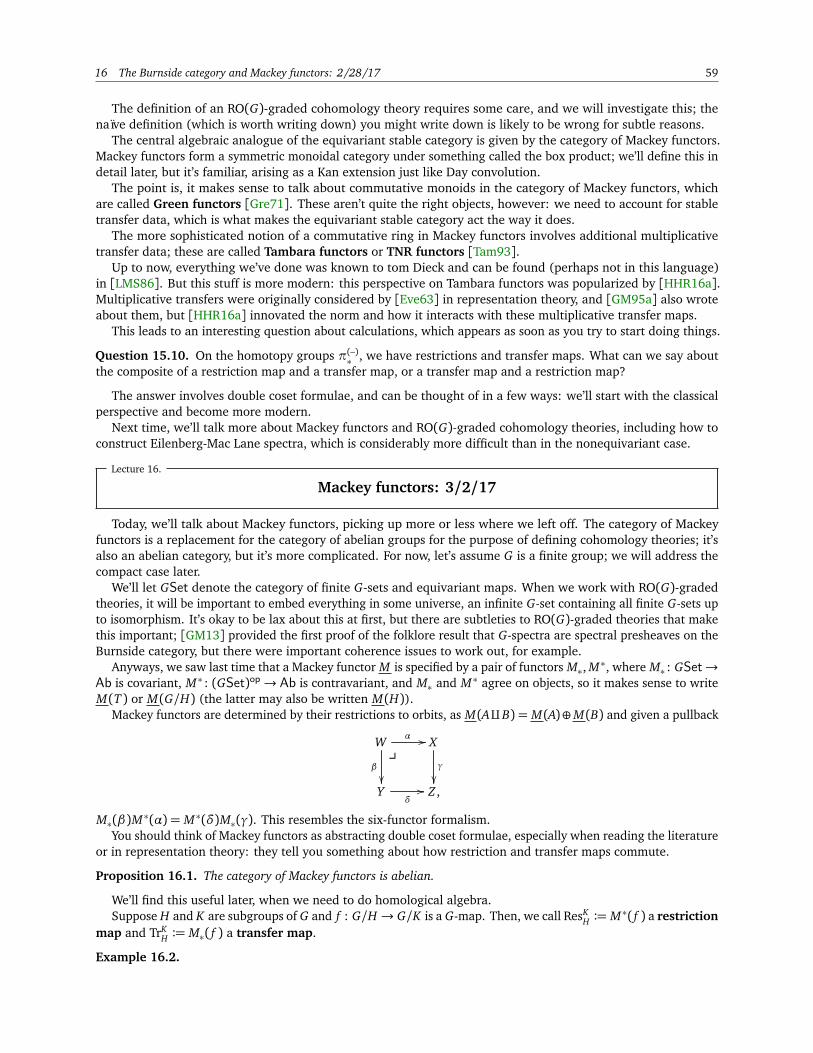
16 The Burnside category and Mackey functors: 2/28/17 59
The definition of an RO(G)-graded cohomology theory requires some care, and we will investigate this; thenaïve definition (which is worth writing down) you might write down is likely to be wrong for subtle reasons.
The central algebraic analogue of the equivariant stable category is given by the category of Mackey functors.Mackey functors form a symmetric monoidal category under something called the box product; we’ll define this indetail later, but it’s familiar, arising as a Kan extension just like Day convolution.
The point is, it makes sense to talk about commutative monoids in the category of Mackey functors, whichare called Green functors [Gre71]. These aren’t quite the right objects, however: we need to account for stabletransfer data, which is what makes the equivariant stable category act the way it does.
The more sophisticated notion of a commutative ring in Mackey functors involves additional multiplicativetransfer data; these are called Tambara functors or TNR functors [Tam93].
Up to now, everything we’ve done was known to tom Dieck and can be found (perhaps not in this language)in [LMS86]. But this stuff is more modern: this perspective on Tambara functors was popularized by [HHR16a].Multiplicative transfers were originally considered by [Eve63] in representation theory, and [GM95a] also wroteabout them, but [HHR16a] innovated the norm and how it interacts with these multiplicative transfer maps.
This leads to an interesting question about calculations, which appears as soon as you try to start doing things.
Question 15.10. On the homotopy groups π(–)∗ , we have restrictions and transfer maps. What can we say aboutthe composite of a restriction map and a transfer map, or a transfer map and a restriction map?
The answer involves double coset formulae, and can be thought of in a few ways: we’ll start with the classicalperspective and become more modern.
Next time, we’ll talk more about Mackey functors and RO(G)-graded cohomology theories, including how toconstruct Eilenberg-Mac Lane spectra, which is considerably more difficult than in the nonequivariant case.
Lecture 16.
Mackey functors: 3/2/17
Today, we’ll talk about Mackey functors, picking up more or less where we left off. The category of Mackeyfunctors is a replacement for the category of abelian groups for the purpose of defining cohomology theories; it’salso an abelian category, but it’s more complicated. For now, let’s assume G is a finite group; we will address thecompact case later.
We’ll let GSet denote the category of finite G-sets and equivariant maps. When we work with RO(G)-gradedtheories, it will be important to embed everything in some universe, an infinite G-set containing all finite G-sets upto isomorphism. It’s okay to be lax about this at first, but there are subtleties to RO(G)-graded theories that makethis important; [GM13] provided the first proof of the folklore result that G-spectra are spectral presheaves on theBurnside category, but there were important coherence issues to work out, for example.
Anyways, we saw last time that a Mackey functor M is specified by a pair of functors M∗, M∗, where M∗ : GSet→Ab is covariant, M∗ : (GSet)op→ Ab is contravariant, and M∗ and M∗ agree on objects, so it makes sense to writeM(T ) or M(G/H) (the latter may also be written M(H)).
Mackey functors are determined by their restrictions to orbits, as M(AqB) = M(A)⊕M(B) and given a pullback
Wù
α //
β
X
γ
Y
δ// Z ,
M∗(β)M∗(α) = M∗(δ)M∗(γ). This resembles the six-functor formalism.You should think of Mackey functors as abstracting double coset formulae, especially when reading the literature
or in representation theory: they tell you something about how restriction and transfer maps commute.
Proposition 16.1. The category of Mackey functors is abelian.
We’ll find this useful later, when we need to do homological algebra.Suppose H and K are subgroups of G and f : G/H → G/K is a G-map. Then, we call ResK
H := M∗( f ) a restrictionmap and TrK
H := M∗( f ) a transfer map.
Example 16.2.

60 M392C (Topics in Algebraic Topology) Lecture Notes
(1) Let X be a G-space. Then, π(–)n (X ), the functor sending G/H 7→ πHn (X ), is a Mackey functor: by the
Wirthmüller isomorphism and the fact that orbits are self-dual,
πHn (X )
∼= [Sn ∧ G/H+, X ]∼= [Sn, X ∧ G/H+],
so it’s clear how a map G/H → G/K induces both a right-way and a wrong-way map.(2) Let Z denote the constant Mackey functor in Z, which assigns Z to every object. The restriction maps
are all the identity, and the transfer G/H → G/K is multiplication by |H/K |.(3) The Burnside Mackey functor A(G) is defined by letting A(G)(G/H) be the Grothendieck group of the
symmetric monoidal category of finite H-sets under coproduct. The transfer and restriction maps comefrom induction and restriction, respectively, between HSet and KSet.
(4) The representation Mackey functor R(G) is defined by letting R(G)(G/H) be the Grothendieck group offinite-dimensional H-representations, with transfer and restriction given by Z[K]⊗Z[H] –. (
The representation Mackey functor contains the information of double coset formulae in representation theory.Namely, suppose H and K are subgroups of G contained in a common subgroup J ⊆ G. The universal property ofthe product gives us a pullback diagram
J/H × J/Kù
//
J/K
J/H // J/J .
If you apply induction to this, you obtain
(16.3)
G ×J (J/H × J/K) //
G ×J (J/K)∼= G/K
G/H // G/J .
As a finite G-set, J/H × J/K is a coproduct of orbits, determined by their stabilizers.
Exercise 16.4. Compute the stabilizer of a point in G/H × G/K , therefore proving that
J/H × J/K ∼=∐
X∈[H\J/K]
G/(H ∩ xK x−1).
This is good practice for working with double cosets, and how group-theoretically, they behave much like ordinarycosets.
Thus (16.3) becomes
(16.5)
∐
X∈[H\J/K]
G/(H ∩ xK x−1)f2 //
f1
G/K
G/H // G/J .
The point is that explicitly determining what f1 and f2 are will produce the double coset formulae. Since H∩ xK x−1
is a subgroup of K , we have a map G/(H ∩ xK x−1)→ G/H, and taking the coproduct over x ∈ [K\J/H] we obtainf1.
f2 is harder, but not much harder: after conjugating by x , we obtain a map G/(x−1H x ∩ K)→ G/K, so f2 isconjugation followed by the natural map.
This means that you can compute how ReskH and TrK
H interact by looking at the two ways around the diagramfrom G/H to G/K , using the restriction and transfer maps for contravariance and covariance, respectively.
(16.6) ResGK TrG
H =⊕
x∈H\G/KTrK
H∩xK x−1 cx ResHH∩xK−1 x ,
where cx is the conjugation map.

16 Mackey functors: 3/2/17 61
Remark. Some treatments define a Mackey functor directly in terms of the restriction and transfer maps withaxioms including the double coset formula (16.6). The more abstract approach we took follows [Dre71], whileolder treatments take the axiomatic approach. In general, the proofs of properties of Mackey functors are sketchedor left out in the literature, but [Web00] and [CITE ME: Devinatz] are pretty good references. (
RO(G)-graded cohomology theories. In the back of your mind, you should be wondering about the connectionbetween G-spectra, equivariant cohomology theories, and Mackey functors. In the nonequivariant setting, Brownrepresentability establishes an (almost) equivalence between spectra and cohomology theories. Equivariantly,things are very similar: G-spectra play the role of spectra, equivariant cohomology theories play the role ofcohomology theories, and, less tautologically, Mackey functors play the role of abelian groups. We’ll talk aboutrings later.
Roughly speaking, an RO(G)-graded cohomology theory should be some collection of functors Eα indexed byα ∈ RO(G) such that for any G-representation V , Eα(X )∼= Eα+V (ΣV X ), and any fixed α should satisfy the wedgeand cofiber axioms, taking wedge products to coproducts and cofiber sequences to long exact sequences.
The (well, an) issue that makes this tricky is that you can’t really work with isomorphism classes of repre-sentations, even though you need that to define RO(G). As a workaround, let’s fix a G-universe U and defineRO(G; U) to be the category whose objects are finite-dimensional representations V that embed equivariantly in Uand whose morphisms V →W are G-equivariant isometric isomorphisms.57 We say that two maps f , g : V →Ware homotopic if their one-point compactifications f , g : SV → SW are stably homotopic. We don’t have enoughstructure to set up a model category or anything, but we can define the homotopy category Ho(RO(G; U)) bypassing to homotopy classes of maps.
A finite-dimensional G-representation defines a suspension functor
ΣW : Ho(RO(G; U))×Ho(GTop) −→ Ho(RO(G; U))×Ho(GTop)
which sends(V, X ) 7−→ (V ⊕W,ΣW X ).
This feels a lot like ordinary SW -suspension, but we’re keeping track of the automorphisms of W .
Definition 16.7. An RO(G)-graded cohomology theory is a functor E : Ho(RO(G; U)) × Ho(GTop)op → Ab,where E(V, X ) is generally written EV (X ), together with isomorphisms
σW : EV (X ) −→ EV⊕W (ΣW X ),
such that for each V , EV (–) satisfies the wedge and cofiber axioms and for each isometric isomorphism α: W →W ′,the map
EV (X )σW //
σW ′
EV⊕W (ΣW X )
(id⊕α,id)
EV⊕W ′(ΣW ′
X )(id⊕id,α)// EV⊕W ′
(ΣW X ).
We further require that σ0 = id and the σW are transitive: σW σV = σV⊕W .
Definition 16.8. The formal differences of objects in RO(G; U) are equivalence classes of pairs (V, W ) of objectsin RO(G; U), where (V, W )∼ (V ′, W ′) if V ⊕W ′ ∼= V ′ ⊕W . The pair (V, W ) is also denoted V W .
We can extend an RO(G; U)-graded cohomology theory to formal differences by EVW (X ) := EV (ΣW X ).Let τ: V ⊕W →W ⊕ V be the transposition natural isomorphism. Then, the coherence condition on the σ(–)
means that the diagram
EV (ΣW X ) //
EV⊕W ′(ΣW⊕W ′X )
τ∗
EV ′(Σ
W ′X ) // EV ′⊕W (Σ
W ′⊕W X )
commutes.
57The data of the embedding V ,→ U is not used in RO(G; U). When we discuss multiplicative structures, this will change.

62 M392C (Topics in Algebraic Topology) Lecture Notes
Remark. When you add ring structures to this story, the coherence conditions become gnarlier: there’s a cocyclearising from the pentagon diagram for associativity. Unfortunately, this is not treated well in the literature; Lewis’thesis [Lew78] discusses it, but was not fully published. [LM06, Appendix A] talks about it, and [CITE ME: Dugger]worked it out in the abstract in the motivic setting. (
We’ll also need to talk about the equivalence between SpG and RO(G)-graded cohomology theories; one directionis Brown representability, and the other is more or less straightforward.
You may be asking why we use RO(G)-graded theories at all. One great reason is that there are known examplesof Z-graded cohomology theories that are extremely chaotic, but the RO(G)-graded theories have nice patterns.Another, more recent, realization is that in many cases the RO(G)-graded theories carry more useful information.However, of course, they’re extremely hard to compute.
Lecture 17.
Brown representability: 3/7/17
“I thought it was obvious, but it’s obviously not obvious.”
Today, we’re going to finish the additive correspondence between G-spectra and RO(G)-graded cohomologytheories, through Neeman’s proof of Brown representability. There will be no class Thursday, so we’ll resume afterspring break with some computations of RO(G)-graded cohomology theories, including ordinary cohomology andhopefully also twisted K-theory.
Anyways, recall that we defined RO(G)-graded cohomology theories EVG (X ) to be Mackey functors graded on
the category RO(G; U), where U is the ambient universe, together with isomorphisms σW : EVG (X )
∼= EV⊕WG (ΣW X ),
together with some additional data.Before we go on, though, we should talk a little about RO(G).
Definition 17.1. Let G be a group and R be a ring. Then, the representation ring of G over R is the Grothendieckconstruction applied to the category of finite-rank G-representations over R, i.e. the ring generated by isomorphismclasses of finite-rank G-representations over R, with the relations [V ⊕W ] = [V ]⊕ [W ] and [V ⊗W ] = [V ] · [W ].58
By the representation ring, we’ll mean RO(G) := R(G), the ring of real representations.
We can think of R(G) and C(G) as rings of characters: given a representation V , its character is the mapχV : G → R (or to C) where χV (g) = tr(g·). Since χV⊕W = χV + χW , χV⊗W = χV · χW , and for irreduciblerepresentations, χV = χW iff V ∼=W , then the characters detect isomorphism classes, so R(G) and C(G) can bethought of as the rings of functions G→ R (resp. C) that are characters.
Exercise 17.2.
(1) Compute C(G) for G = Cp, and then for Cm where m isn’t prime.(2) Harder: compute R(G) for the same G.
One of the important connections in ordinary stable homotopy theory is that cohomology theories are closelyrelated to spectra: every spectrum determines a cohomology theory, and up to a very small ambiguity, a cohomologytheory is represented by a spectrum.
Definition 17.3. Let E be a G-spectrum. Then, we define E-cohomology to be the functor EVG (X ) := [SV ∧ X , E]G .
This is an RO(G)-graded cohomology theory, but this is something to check. If you want to restrict your universe,there are some nuances that have to be overcome.
If you put in finite G-sets (basically points), what you get is a Mackey functor: considering maps out of Xensures the transfer maps have the correct variance.
That was the easy direction: the other direction requires Brown representability. This is originally due to[Bro62], and we’ll give Neeman’s interpretation [Nee96]. It works in any triangulated category, and is very closeto the small object argument, which already makes it a good thing.
Fix a triangulated category C that has small coproducts. The stable homotopy categories Ho(Sp) and Ho(SpG)are the examples to keep in mind.
58Not every element of R(G) is the class of a representation: some elements are formal differences of two representations. These elementsare sometimes called virtual representations.

17 Brown representability: 3/7/17 63
Definition 17.4. An x ∈ C is compact if for all countable coproducts over yi ∈ C,
MapC
x ,∐
i
yi
∼=∐
i
MapC(x , yi).
This is not the usual definition of compactness in category theory, which uses filtered colimits, but in thestable setting these are the same as coproducts, motivating our definition. For example, this definition does notcharacterize compact topological spaces.
Definition 17.5.• A generating set of a category C is a set T ⊆ ob(C) that detects zero, i.e. for all x ∈ C, x = 0 iff
MapC(z, x) = 0 for all z ∈ T . If C is triangulated, we additionally require T to be closed under shift.• C is compactly generated if it has a generating set consisting of compact objects.
We introduce these to skate around set-theoretic issues: at some point, we’d like to take a coproduct over allobjects in the category, but that’s too large. Instead, taking the coproduct over all generators will have the samepower, and is actually well-defined.
For example, dualizable spectra (resp. dualizable G-spectra) are a compact generating set for Ho(Sp) (resp.Ho(SpG)).
Theorem 17.6 (Brown representability [Bro62, Nee96]). Let C be a compactly generated triangulated category andH : Cop→ Ab be a functor such that
(1)
H
∐
i
X i
∼=∏
i
H(X i)
and(2) H sends exact triangles X → Y → Z → X [1] to long exact sequences
H(X ) // H(Y ) // H(Z) // H(X [1]) // H(Y [1]) // H(Z[1]) // H(X [2]) // · · ·
Then, H is representable, i.e. there’s an X ∈ C and a natural isomorphism HomC(–, X )→ H.
Proof. We’re going to build X inductively. Fix a generating set T for C of compact objects.In the base case, let
U0 :=∐
x∈T
H(x) and X0 :=∐
(α,t)∈U0α∈H(t)
t.
Thus,
H(X0) = H
∐
(α,t)∈U0
t
!
∼=∏
(α,t)∈U0
H(t),
and in particular there is a distinguished element α0 ∈ H(X0) which is α at the (α, t) factor. By the Yoneda lemma,α0 specifies a natural transformation θ0 : MapC(–, X0)→ H, and by construction, θ0 is surjective for each t ∈ T .
Now we induct: assume we have X i and αi specifying a natural transformation θi : MapC(–, X i)→ H. Then,define
Ui+1 :=∐
t∈T
ker(θi(t): MapC(t, X i)→ H(t)). and Ki+1 :=∐
( f ,t)∈Ui+1
t.
There’s a natural map Ki+1→ X i which applies f ; let X i+1 be its cofiber. Applying H, this produces a map
H(X i+1) // H(X i) // H(Ki+1),
and by construction, αi 7→ 0, so by exactness, we can lift to αi+1 ∈ H(X i+1). This αi+1 specifies a naturaltransformation θi+1 : MapC(–, X i+1)→ H, and the following diagram commutes:
MapC(–, X i)θi //
H
MapC(–, X i+1).θi+1
99
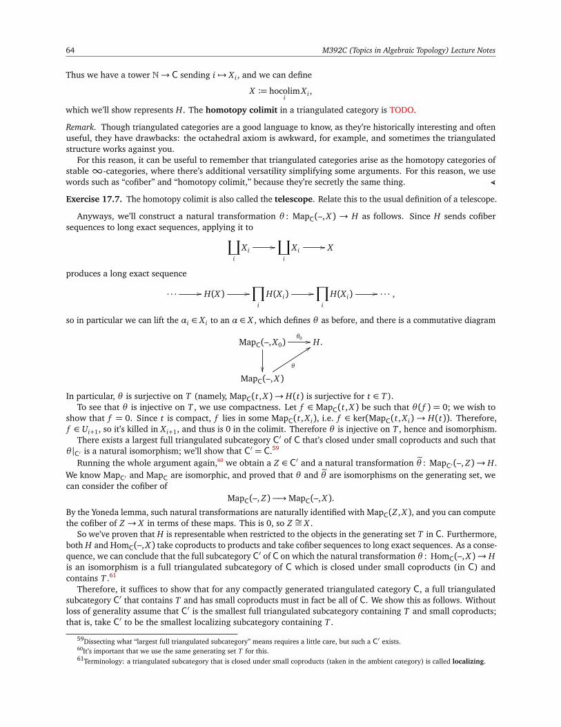
64 M392C (Topics in Algebraic Topology) Lecture Notes
Thus we have a tower N→ C sending i 7→ X i , and we can define
X := hocolimi
X i ,
which we’ll show represents H. The homotopy colimit in a triangulated category is TODO.
Remark. Though triangulated categories are a good language to know, as they’re historically interesting and oftenuseful, they have drawbacks: the octahedral axiom is awkward, for example, and sometimes the triangulatedstructure works against you.
For this reason, it can be useful to remember that triangulated categories arise as the homotopy categories ofstable∞-categories, where there’s additional versatility simplifying some arguments. For this reason, we usewords such as “cofiber” and “homotopy colimit,” because they’re secretly the same thing. (
Exercise 17.7. The homotopy colimit is also called the telescope. Relate this to the usual definition of a telescope.
Anyways, we’ll construct a natural transformation θ : MapC(–, X ) → H as follows. Since H sends cofibersequences to long exact sequences, applying it to
∐
i
X i//∐
i
X i// X
produces a long exact sequence
· · · // H(X ) //∏
i
H(X i) //∏
i
H(X i) // · · · ,
so in particular we can lift the αi ∈ X i to an α ∈ X , which defines θ as before, and there is a commutative diagram
MapC(–, X0)θ0 //
H.
MapC(–, X )θ
::
In particular, θ is surjective on T (namely, MapC(t, X )→ H(t) is surjective for t ∈ T).To see that θ is injective on T , we use compactness. Let f ∈ MapC(t, X ) be such that θ( f ) = 0; we wish to
show that f = 0. Since t is compact, f lies in some MapC(t, X i), i.e. f ∈ ker(MapC(t, X i)→ H(t)). Therefore,f ∈ Ui+1, so it’s killed in X i+1, and thus is 0 in the colimit. Therefore θ is injective on T , hence and isomorphism.
There exists a largest full triangulated subcategory C′ of C that’s closed under small coproducts and such thatθ |C′ is a natural isomorphism; we’ll show that C′ = C.59
Running the whole argument again,60 we obtain a Z ∈ C′ and a natural transformation eθ : MapC′(–, Z)→ H.We know MapC′ and MapC are isomorphic, and proved that θ and eθ are isomorphisms on the generating set, wecan consider the cofiber of
MapC(–, Z) −→MapC(–, X ).
By the Yoneda lemma, such natural transformations are naturally identified with MapC(Z , X ), and you can computethe cofiber of Z → X in terms of these maps. This is 0, so Z ∼= X .
So we’ve proven that H is representable when restricted to the objects in the generating set T in C. Furthermore,both H and HomC(–, X ) take coproducts to products and take cofiber sequences to long exact sequences. As a conse-quence, we can conclude that the full subcategory C′ of C on which the natural transformation θ : HomC(–, X )→ His an isomorphism is a full triangulated subcategory of C which is closed under small coproducts (in C) andcontains T .61
Therefore, it suffices to show that for any compactly generated triangulated category C, a full triangulatedsubcategory C′ that contains T and has small coproducts must in fact be all of C. We show this as follows. Withoutloss of generality assume that C′ is the smallest full triangulated subcategory containing T and small coproducts;that is, take C′ to be the smallest localizing subcategory containing T .
59Dissecting what “largest full triangulated subcategory” means requires a little care, but such a C′ exists.60It’s important that we use the same generating set T for this.61Terminology: a triangulated subcategory that is closed under small coproducts (taken in the ambient category) is called localizing.

18 Brown representability: 3/7/17 65
Now fix an object c ∈ C and consider the functor HomC(–, c). Applying the construction from above, we obtainan object z and a natural transformation HomC(–, z)→ HomC(–, c). By construction, the object z ∈ C′ — each X iis in C′, and so the homotopy colimit is too. Moreover, the map HomC(t, z)→ HomC(t, c) is an isomorphism forall t ∈ T .
The Yoneda lemma now implies that we have a map z→ c which corresponds to the natural transformationHomC(–, z)→ HomC(–, c). Consider the cofiber c/z. By the previous paragraph and the fact that HomC(t, –) takestriangles to long exact sequences, HomC(t, c/z) = 0 for all t ∈ T , and so c/z = 0. Therefore c and z are isomorphic.Since z is in C′, c ∈ C′. As c was chosen arbitrarily, we conclude that C and C′ coincide.
Next time, we’ll discuss what Brown representability means for G-spectra, and use it to define Eilenberg-MacLane spectra as the spectra representing certain cohomology theories. One fun fact about G-spectra is that everyZ-graded cohomology theory uniquely extends to an RO(G)-graded cohomology theory by taking shifts, but this isnot true for G-spaces!
Lecture 18.
Eilenberg-Mac Lane spectra: 3/21/17
“The large print giveth and the small print taketh away.”The big goal of today’s lecture is to construct Eilenberg-Mac Lane spectra: if M is a Mackey functor, we’ll producea G-spectrum HM which represents ordinary cohomology with coefficients in M . This will take some work, butwill have some nice payoffs. We’ll begin some computations: for G = C2, we’ll compute the Bredon cohomologyHC2(∗;Z) and HC2
(∗; A), where Z is the constant Z-valued Mackey functor and A is the Burnside Mackey functor(Example 16.2).
Last time, we proved Brown representability (Theorem 17.6) for triangulated categories, which are stable. Wealso want an unstable variant.
Theorem 18.1 (Unstable Brown representability). Let C denote the category of based, G-connected G-CW complexesand H : Ho(C)op→ Set be a functor such that
(1) H satisfies the wedge axioms, and(2) H takes homotopy pushouts to (weak) pullbacks.
Then, H is represented, and the converse is true.
Though we stated this theorem for H going to Set, it turns out all such functors factor through the forgetfulfunctor Ab→ Set, and therefore can be taken to be Ab-valued.
Warning! The basepoint and connectivity hypotheses are important: Brown representability does not hold in theunstable case if you fail to impose those requirements.
We can use Brown representability to prove the following result.
Proposition 18.2. Any RO(G)-graded cohomology theory is represented by a G-spectrum.
Proof. Let E be an RO(G)-graded cohomology theory. We can apply Brown representability to EVG (–) for each V ,
and the identification EVG (Σ
W X ) ∼= EV⊕WG (X ) gives rise to a homotopy class of structure maps on representing
objects, but there’s a coherence issue: we constructed G-spectra with actual structure maps, not homotopy classesof maps.
The usual way to solve this is with a trick: restrict attention to a cofinal indexing sequence Vn ,→ Vn+1 ,→Vn+2 ,→ . . . , and then observe that the homotopy theory of G-prespectra on this sequence is equivalent to Ho(SpG),which is guaranteed by cofinality: limits are preserved, and the homotopy groups are the same. This fixes thecoherence problem: we can pick a representative for each map and force transitivity. Then, we can left Kan extendback to an orthogonal G-spectrum.
This would be an exercise, except that maybe it’s a bit too hard to be one.
Question 18.3. Can we build an object of SpG directly? It would be nice not to worry about prespectra on acofinal sequence.
There are different ways to think about doing this. One approach goes through the model of the G-stablecategory as spectral presheaves.

66 M392C (Topics in Algebraic Topology) Lecture Notes
This provides the connection between cohomology theories on G-spaces and G-spectra, just like in the nonequiv-ariant world. They’re almost the same, except for the existence of phantom maps,62 just like in the nonequivariantcase. These are poorly understood, but of course we want to understand them better in the nonequivariant case.
Corollary 18.4. A Z-graded cohomology theory on SpG is represented by an object of SpG .
The proof is that ΣV and ΩV are inverse equivalences in Ho(SpG), so we can use them to extend to RO(G)-gradedtheories. Corollary 18.4 feels like a weird coincidence, but it’s a key technical result that we’ll use more than once.The unstable case is different, though.
Corollary 18.5. A Z-graded cohomology theory on GTop with coefficients in a coefficient system M extends to anRO(G)-graded theory iff M extends to (the contravariant part of) a Mackey functor.
Now we can build Eilenberg-Mac Lane spectra for a Mackey functor M . There will be two constructions: onemay be more satisfying. You might hope to use obstruction theory to build Eilenberg-Mac Lane spaces and chainthem together, but this is a mess. We’ll adopt one unfamiliar-looking approach, which always works, and also seea more familiar one.
Construction 18.6. Given M , we’ll construct a Z-graded cohomology theory on SpG; by Corollary 18.5, this isrepresented by an object of SpG , which will be HM .
Let X be a G-CW complex, and define Cn(X ) := πn(Xn/Xn−1) (where Xn is the n-skeleton of X ). Now we’llreplicate the construction of Bredon cohomology; in particular, the long exact sequence for the triple (Xn, Xn−1, Xn−2)induces a differential Cn(X )→ Cn−1(X ). If Mac denotes the category of Mackey functors, consider the cochaincomplex
HomMac(Cn(X ), M),
and take the cohomology of this cochain complex.This is represented by an Eilenberg-Mac Lane spectrum HM ∈ SpG , and one can calculate that
πHk (HM) =
¨
0, k 6= 0
M(G/H), k = 0.
From this perspective, it’s easy to show that H is functorial, which is nice. But you might wonder if it’s symmetricmonoidal: in the nonequivariant case, H(R⊗ S) ' HR∧ HS. This is false, and is one of the unfortunate thingsabout the equivariant setting.
Though the cohomology theory HM represents is explicit, the spectrum itself is not. Brown’s original proofof Brown representability [Bro62] looks a lot like Postnikov induction, which closely resembles one classicalconstruction of nonequivariant Eilenberg-Mac Lane spaces, which suggests a more explicit approach is possible.
Construction 18.7. One can build some Eilenberg-Mac Lane spectra via the equivariant Dold-Thom construction;this approach only works in certain settings (we’ll say which ones in a bit), but is interesting enough to mention.
First let’s discuss the nonequivariant case. Let Sp∞ : Top∗→ TopCMon be the free functor from based spacesto topological abelian monoids (i.e. adjoint to the forgetful functor). The proof of Dold-Thom amounts to checkthat Sp∞ is a fibrantW -space, which means checking that it takes homotopy pushouts to homotopy pullbacks. Wecan identify this with HZ.
We’ll now introduce the McCord construction. McCord’s original paper [McC69] is a good reference. NickKuhn has a talent for clarifying constructions and finding cool uses for them, and his paper [Kuh04b] on theMcCord construction is also great.
Let A be an abelian group and X be a based space. Let A⊗ X denote the free abelian topological monoid onpairs (a, x), written xa, subject to the relations
(1) ∗a = ∗,(2) x0 = ∗, and(3) xa x b = xa+b.
That is, Y inherits the quotient topology from the free abelian topological monoid.
62A phantom map is a nonzero morphism between spectra that’s not detected by any compact object. In particular, this means that asa natural transformation of cohomology theories, it’s 0, but arises from a nonzero morphism. These encode the non-uniqueness of Brownrepresentability.

18 Eilenberg-Mac Lane spectra: 3/21/17 67
Remark. The McCord construction can be carried out very generally, e.g. Kuhn [Kuh04b] uses a closely relatedmodel to analyze the categorical tensor product in ring spectra. (
One can prove a version of the Dold-Thom theorem that implies that A⊗ – is a model for HA. This is aW -space, and we can think of this as A⊗ Sn. There’s also a Γ -space n 7→ n⊗ A, and one can check this is fibrant,i.e. very special.
In our case, suppose M is a Z[G]-module, and that G is finite. We can extract a Mackey functor M(G/H) := M H ,where the transfer TrK
H sends
x 7−→∑
hH∈K/H
hx .
You can check this is a Mackey functor. The equivariant McCord construction produces Eilenberg-Mac Lanespectra for the Mackey functors that arise in this way; see dos Santos [dS03], dos Santos-Nie [dSN09], orShimakawa [Shi89].
If A is a based G-space and M is a Z[G]-module, then A⊗M is a G-space using the diagonal G-action. Whatyou obtain is an equivariant Γ -space. We haven’t talked much about these, and we won’t, but they’re interesting.Segal’s preprint on equivariant Γ -spaces [Seg78] is highly influential and widely circulated, but the statement hasa mistake (though the proof is correct).
Exercise 18.8. Find the mistake, and fix it. At this point, you have the background to do so.
[Shi89] wrote up the correction, and [Blu06] answers a related question about equivariant W -spaces.
Theorem 18.9. SV ⊗M is a model of HM.
So this construction is nice and explicit, but only works when G is finite, and for Mackey functors that arisefrom Z[G]-modules.
Understanding the Dold-Thom construction is equivalent to understanding infinite loop space theory, and forgeneral compact Lie groups we understand neither.
There aren’t many examples of calculations in Bredon cohomology, except for what people needed for otherthings: Stong has some lecture notes which might be published, and the motivic homotopy theorists (specificallyDugger and Voevodsky) used the C2-equivariant category as a model for the motivic setting, and wrote up somecalculations. See, e.g., [Lew88, Dug15].
The takeaway is that, even for groups such as C4, calculating the Bredon cohomology of a point would almostbe a paper. People probably know what it is, but it would be interesting to understand. The equivariant Steenrodand Dyer-Lashof algebras are also not understood well; Hill-Hopkins-Ravenel figured some of it out, but might nothave written all of it down. This would be hard to attack via a Cartan-style seminar, unfortunately.
Thus, it’s not at all trivial that we’re computing H∗C2(∗;Z). Recall that Z comes from the coefficient system
M(C2/C2)
M(C2/e),
OO
WW
but as a Mackey functor there’s also a transfer map f∗:
M(C2/C2)
f∗
M(C2/e).
f ∗
DD
γ
WW
Exercise 18.10. Show that the double coset formulae force f∗ f ∗ = 1+ γ and f ∗ f∗ = 2.63
For Z,63TODO: I’d like to double-check that I got this correct.
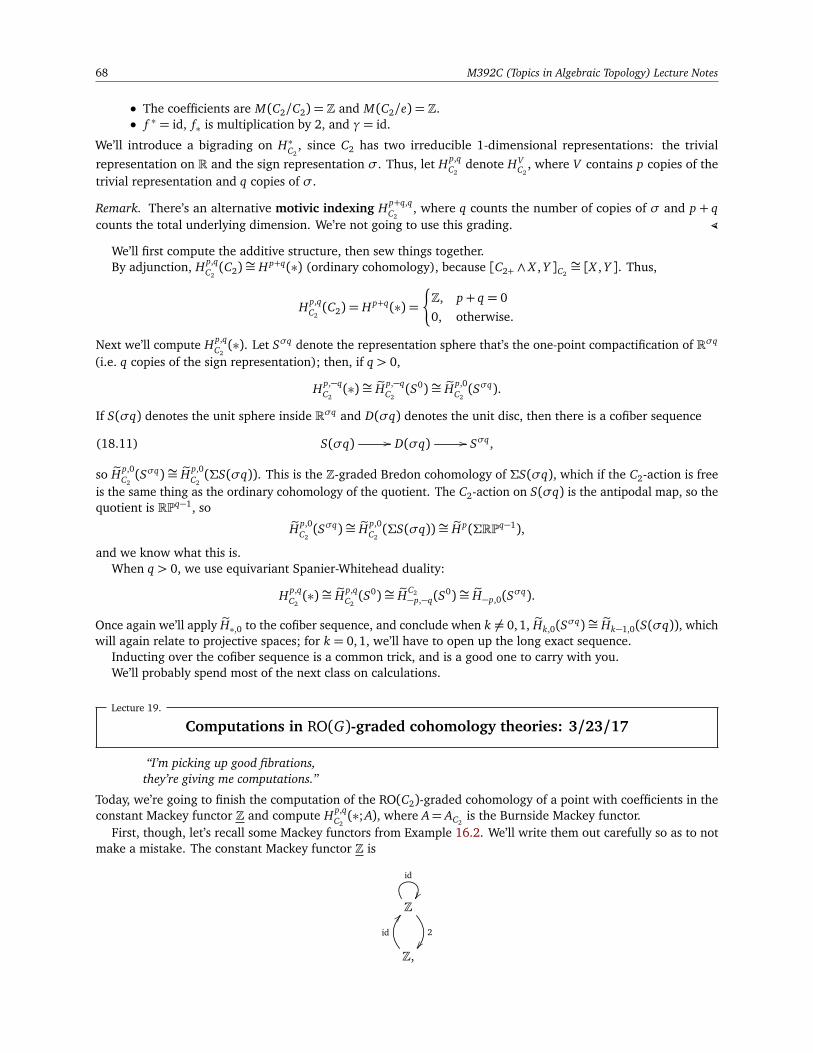
68 M392C (Topics in Algebraic Topology) Lecture Notes
• The coefficients are M(C2/C2) = Z and M(C2/e) = Z.• f ∗ = id, f∗ is multiplication by 2, and γ= id.
We’ll introduce a bigrading on H∗C2, since C2 has two irreducible 1-dimensional representations: the trivial
representation on R and the sign representation σ. Thus, let H p,qC2
denote HVC2
, where V contains p copies of thetrivial representation and q copies of σ.
Remark. There’s an alternative motivic indexing H p+q,qC2
, where q counts the number of copies of σ and p + qcounts the total underlying dimension. We’re not going to use this grading. (
We’ll first compute the additive structure, then sew things together.By adjunction, H p,q
C2(C2)∼= H p+q(∗) (ordinary cohomology), because [C2+ ∧ X , Y ]C2
∼= [X , Y ]. Thus,
H p,qC2(C2) = H p+q(∗) =
¨
Z, p+ q = 0
0, otherwise.
Next we’ll compute H p,qC2(∗). Let Sσq denote the representation sphere that’s the one-point compactification of Rσq
(i.e. q copies of the sign representation); then, if q > 0,
H p,−qC2(∗)∼= eH p,−q
C2(S0)∼= eH p,0
C2(Sσq).
If S(σq) denotes the unit sphere inside Rσq and D(σq) denotes the unit disc, then there is a cofiber sequence
(18.11) S(σq) // D(σq) // Sσq,
so eH p,0C2(Sσq)∼= eH p,0
C2(ΣS(σq)). This is the Z-graded Bredon cohomology of ΣS(σq), which if the C2-action is free
is the same thing as the ordinary cohomology of the quotient. The C2-action on S(σq) is the antipodal map, so thequotient is RPq−1, so
eH p,0C2(Sσq)∼= eH p,0
C2(ΣS(σq))∼= eH p(ΣRPq−1),
and we know what this is.When q > 0, we use equivariant Spanier-Whitehead duality:
H p,qC2(∗)∼= eH p,q
C2(S0)∼= eHC2
−p,−q(S0)∼= eH−p,0(S
σq).
Once again we’ll apply eH∗,0 to the cofiber sequence, and conclude when k 6= 0, 1, eHk,0(Sσq)∼= eHk−1,0(S(σq)), whichwill again relate to projective spaces; for k = 0,1, we’ll have to open up the long exact sequence.
Inducting over the cofiber sequence is a common trick, and is a good one to carry with you.We’ll probably spend most of the next class on calculations.
Lecture 19.
Computations in RO(G)-graded cohomology theories: 3/23/17
“I’m picking up good fibrations,they’re giving me computations.”
Today, we’re going to finish the computation of the RO(C2)-graded cohomology of a point with coefficients in theconstant Mackey functor Z and compute H p,q
C2(∗; A), where A= AC2
is the Burnside Mackey functor.First, though, let’s recall some Mackey functors from Example 16.2. We’ll write them out carefully so as to not
make a mistake. The constant Mackey functor Z is
Z
2
id
Z,
id
BB
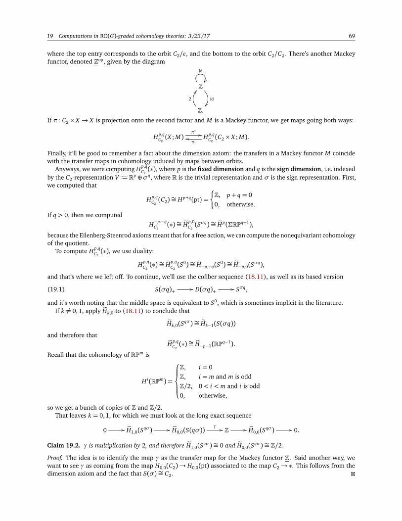
19 Computations in RO(G)-graded cohomology theories: 3/23/17 69
where the top entry corresponds to the orbit C2/e, and the bottom to the orbit C2/C2. There’s another Mackeyfunctor, denoted Zop, given by the diagram
Z
id
id
Z.
2
AA
If π: C2 × X → X is projection onto the second factor and M is a Mackey functor, we get maps going both ways:
H p,qC2(X ; M)
π∗ // H p,qC2(C2 × X ; M).
π!
oo
Finally, it’ll be good to remember a fact about the dimension axiom: the transfers in a Mackey functor M coincidewith the transfer maps in cohomology induced by maps between orbits.
Anyways, we were computing H p,qC2(∗), where p is the fixed dimension and q is the sign dimension, i.e. indexed
by the C2-representation V := Rp ⊕σq, where R is the trivial representation and σ is the sign representation. First,we computed that
H p,qC2(C2)∼= H p+q(pt) =
¨
Z, p+ q = 0
0, otherwise.
If q > 0, then we computed
H−p.−qC2
(∗)∼= eH p,0C2(Sσq)∼= eH p(ΣRPq−1),
because the Eilenberg-Steenrod axioms meant that for a free action, we can compute the nonequivariant cohomologyof the quotient.
To compute H p,qC2(∗), we use duality:
H p,qC2(∗)∼= eH p,q
C2(S0)∼= eH−p,−q(S
0)∼= eH−p,0(Sσq),
and that’s where we left off. To continue, we’ll use the cofiber sequence (18.11), as well as its based version
(19.1) S(σq)+ // D(σq)+ // Sσq,
and it’s worth noting that the middle space is equivalent to S0, which is sometimes implicit in the literature.If k 6= 0,1, apply eHk,0 to (18.11) to conclude that
eHk,0(Sqσ)∼= eHk−1(S(σq))
and therefore thateH p,q
C2(∗)∼= eH−p−1(RPq−1).
Recall that the cohomology of RPm is
H i(RPm) =
Z, i = 0
Z, i = m and m is odd
Z/2, 0< i < m and i is odd
0, otherwise,
so we get a bunch of copies of Z and Z/2.That leaves k = 0,1, for which we must look at the long exact sequence
0 //eH1,0(S
qσ) //eH0,0(S(qσ))
γ // Z //eH0,0(S
qσ) // 0.
Claim 19.2. γ is multiplication by 2, and therefore eH1,0(Sqσ)∼= 0 and eH0,0(Sqσ)∼= Z/2.
Proof. The idea is to identify the map γ as the transfer map for the Mackey functor Z. Said another way, wewant to see γ as coming from the map H0,0(C2)→ H0,0(pt) associated to the map C2→ ∗. This follows from thedimension axiom and the fact that S(σ)∼= C2.
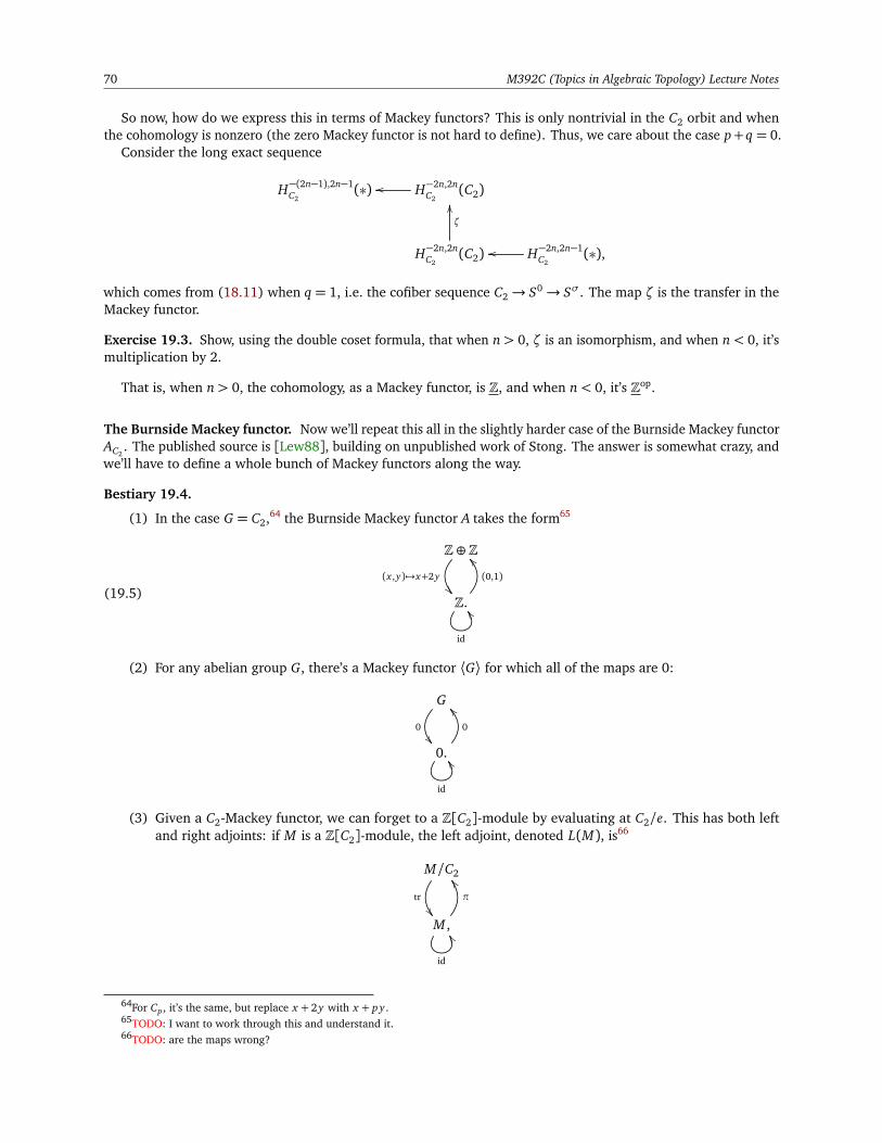
70 M392C (Topics in Algebraic Topology) Lecture Notes
So now, how do we express this in terms of Mackey functors? This is only nontrivial in the C2 orbit and whenthe cohomology is nonzero (the zero Mackey functor is not hard to define). Thus, we care about the case p+q = 0.
Consider the long exact sequence
H−(2n−1),2n−1C2
(∗) H−2n,2nC2
(C2)oo
H−2n,2nC2
(C2)
ζ
OO
H−2n,2n−1C2
(∗),oo
which comes from (18.11) when q = 1, i.e. the cofiber sequence C2→ S0→ Sσ. The map ζ is the transfer in theMackey functor.
Exercise 19.3. Show, using the double coset formula, that when n> 0, ζ is an isomorphism, and when n< 0, it’smultiplication by 2.
That is, when n> 0, the cohomology, as a Mackey functor, is Z, and when n< 0, it’s Zop.
The Burnside Mackey functor. Now we’ll repeat this all in the slightly harder case of the Burnside Mackey functorAC2
. The published source is [Lew88], building on unpublished work of Stong. The answer is somewhat crazy, andwe’ll have to define a whole bunch of Mackey functors along the way.
Bestiary 19.4.
(1) In the case G = C2,64 the Burnside Mackey functor A takes the form65
(19.5)
Z⊕Z
(x ,y)7→x+2yZ.
id
YY
(0,1)
]]
(2) For any abelian group G, there’s a Mackey functor ⟨G⟩ for which all of the maps are 0:
G
00.
id
YY
0
]]
(3) Given a C2-Mackey functor, we can forget to a Z[C2]-module by evaluating at C2/e. This has both leftand right adjoints: if M is a Z[C2]-module, the left adjoint, denoted L(M), is66
M/C2
tr
M ,
id
XX
π
ZZ
64For Cp , it’s the same, but replace x + 2y with x + p y .65TODO: I want to work through this and understand it.66TODO: are the maps wrong?
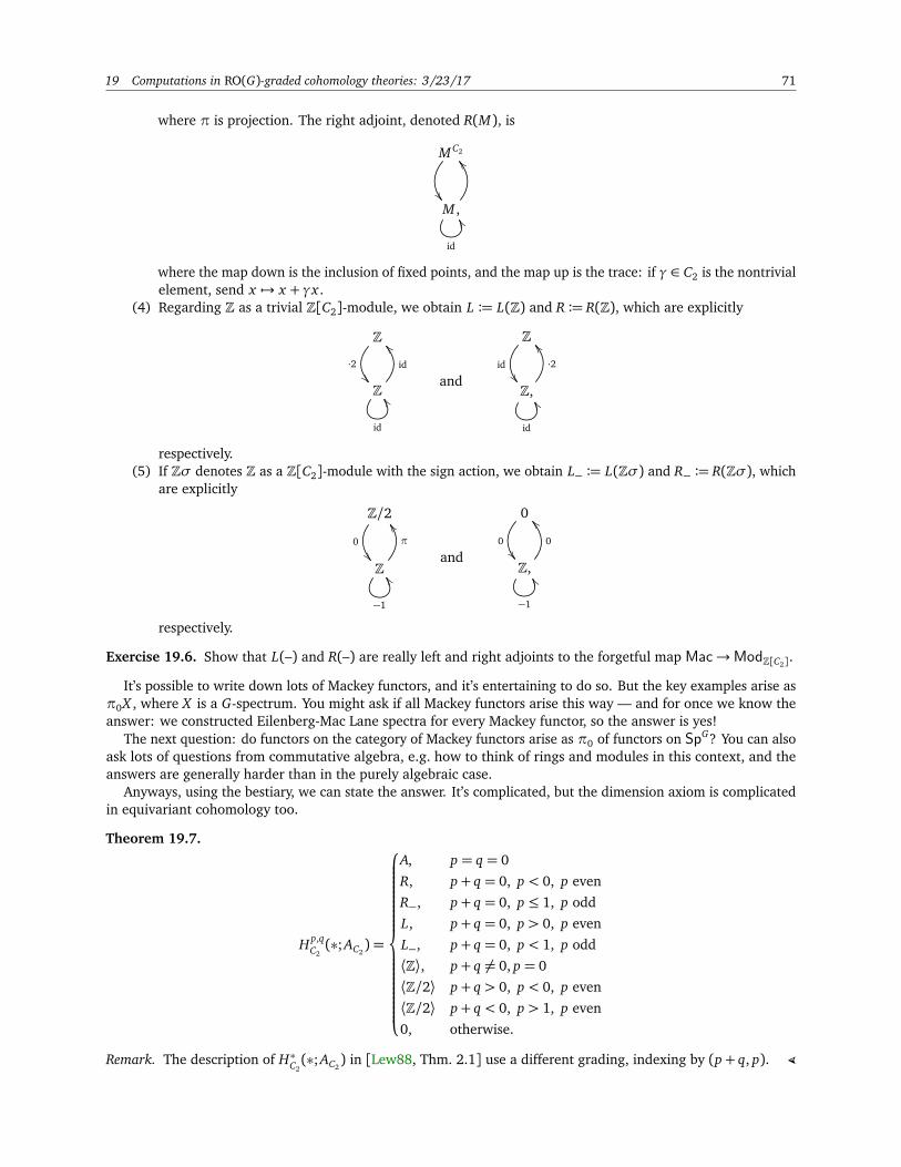
19 Computations in RO(G)-graded cohomology theories: 3/23/17 71
where π is projection. The right adjoint, denoted R(M), is
M C2
M ,
id
XX
\\
where the map down is the inclusion of fixed points, and the map up is the trace: if γ ∈ C2 is the nontrivialelement, send x 7→ x + γx .
(4) Regarding Z as a trivial Z[C2]-module, we obtain L := L(Z) and R := R(Z), which are explicitly
Z
·2Z
id
YY
id
]]
and
Z
idZ,
id
XX
·2
\\
respectively.(5) If Zσ denotes Z as a Z[C2]-module with the sign action, we obtain L− := L(Zσ) and R− := R(Zσ), which
are explicitly
Z/2
0
Z
−1
YY
π
ZZ
and
0
0Z,
−1
XX
0
]]
respectively.
Exercise 19.6. Show that L(–) and R(–) are really left and right adjoints to the forgetful map Mac→ModZ[C2].
It’s possible to write down lots of Mackey functors, and it’s entertaining to do so. But the key examples arise asπ0X , where X is a G-spectrum. You might ask if all Mackey functors arise this way — and for once we know theanswer: we constructed Eilenberg-Mac Lane spectra for every Mackey functor, so the answer is yes!
The next question: do functors on the category of Mackey functors arise as π0 of functors on SpG? You can alsoask lots of questions from commutative algebra, e.g. how to think of rings and modules in this context, and theanswers are generally harder than in the purely algebraic case.
Anyways, using the bestiary, we can state the answer. It’s complicated, but the dimension axiom is complicatedin equivariant cohomology too.
Theorem 19.7.
H p,qC2(∗; AC2
) =
A, p = q = 0
R, p+ q = 0, p < 0, p even
R−, p+ q = 0, p ≤ 1, p odd
L, p+ q = 0, p > 0, p even
L−, p+ q = 0, p < 1, p odd
⟨Z⟩, p+ q 6= 0, p = 0
⟨Z/2⟩ p+ q > 0, p < 0, p even
⟨Z/2⟩ p+ q < 0, p > 1, p even
0, otherwise.
Remark. The description of H∗C2(∗; AC2
) in [Lew88, Thm. 2.1] use a different grading, indexing by (p+ q, p). (
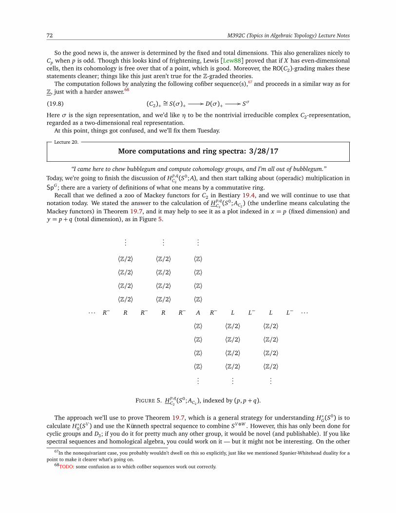
72 M392C (Topics in Algebraic Topology) Lecture Notes
So the good news is, the answer is determined by the fixed and total dimensions. This also generalizes nicely toCp when p is odd. Though this looks kind of frightening, Lewis [Lew88] proved that if X has even-dimensionalcells, then its cohomology is free over that of a point, which is good. Moreover, the RO(C2)-grading makes thesestatements cleaner; things like this just aren’t true for the Z-graded theories.
The computation follows by analyzing the following cofiber sequence(s),67 and proceeds in a similar way as forZ, just with a harder answer.68
(C2)+ ∼= S(σ)+ // D(σ)+ // Sσ(19.8)
Here σ is the sign representation, and we’d like η to be the nontrivial irreducible complex C2-representation,regarded as a two-dimensional real representation.
At this point, things got confused, and we’ll fix them Tuesday.
Lecture 20.
More computations and ring spectra: 3/28/17
“I came here to chew bubblegum and compute cohomology groups, and I’m all out of bubblegum.”Today, we’re going to finish the discussion of H p,q
C2(S0; A), and then start talking about (operadic) multiplication in
SpG; there are a variety of definitions of what one means by a commutative ring.Recall that we defined a zoo of Mackey functors for C2 in Bestiary 19.4, and we will continue to use that
notation today. We stated the answer to the calculation of H p,qC2(S0;AC2
) (the underline means calculating theMackey functors) in Theorem 19.7, and it may help to see it as a plot indexed in x = p (fixed dimension) andy = p+ q (total dimension), as in Figure 5.
......
...
⟨Z/2⟩ ⟨Z/2⟩ ⟨Z⟩
⟨Z/2⟩ ⟨Z/2⟩ ⟨Z⟩
⟨Z/2⟩ ⟨Z/2⟩ ⟨Z⟩
⟨Z/2⟩ ⟨Z/2⟩ ⟨Z⟩
· · · R− R R− R R− A R− L L− L L− · · ·
⟨Z⟩ ⟨Z/2⟩ ⟨Z/2⟩
⟨Z⟩ ⟨Z/2⟩ ⟨Z/2⟩
⟨Z⟩ ⟨Z/2⟩ ⟨Z/2⟩
⟨Z⟩ ⟨Z/2⟩ ⟨Z/2⟩...
......
FIGURE 5. H p,qC2(S0; AC2
), indexed by (p, p+ q).
The approach we’ll use to prove Theorem 19.7, which is a general strategy for understanding H∗G(S0) is to
calculate H∗0(SV ) and use the Künneth spectral sequence to combine SV⊕W . However, this has only been done for
cyclic groups and D3; if you do it for pretty much any other group, it would be novel (and publishable). If you likespectral sequences and homological algebra, you could work on it — but it might not be interesting. On the other
67In the nonequivariant case, you probably wouldn’t dwell on this so explicitly, just like we mentioned Spanier-Whitehead duality for apoint to make it clearer what’s going on.
68TODO: some confusion as to which cofiber sequences work out correctly.
20 More computations and ring spectra: 3/28/17 73
hand, the engine that lets [HHR16a] prove the Kervaire invariant 1 problem is a computation of RO((C2)n)-gradedcohomology of a point with coefficients in constant Mackey functors, which leads to the gap theorem, using amethod Doug Ravenel suggested in the 1970s, so who knows what you could discover?
In our calculation, we’ll exploit the cofiber sequence (19.8) heavily. The first example is the calculation ofH p,q
C2((C2)+).
Proposition 20.1.
H p,qC2((C2)+) =
¨
AC2, p+ q = 0
0, otherwise.
Proof sketch. Let M be an abelian group and M2 denote the Z[C2]-module M ⊕M , where the nontrivial elementof C2 acts by switching the factors.69
Exercise 20.2. Show that L(M2) = R(M2).
We’ll let MC2denote L(M2). If M is a Mackey functor, the notation MC2
means L(M(e)2).Observe that H p,q
C2((C2)+)∼= (H
p,qC2(S0)(e))C2
.
Using the long exact sequence associated to (19.8), the map
H p,q−1C2
(S0)∼= H p,qC2(Sσ) −→ H p,q
C2(S0)
is injective if p+ q 6= 1 and surjective when p+ q 6= 0, hence an isomorphism when p+ q 6= 0,1.Therefore, we conclude that there are 0s in the upper right and lower left quadrants (indexing by (p, p+q) as in
Figure 5): when H p,q−1C2
(S0)∼= H p,qC2(S0), we can pull the σ factors out of the representation and use the dimension
axiom.
Proposition 20.3. When p+ q = 1, we have
H p,qC2(S0)∼= coker
H p,q−1C2
((C2)+) −→ H p,q−1C2
(S0)
and when p+ q = −1,
H p,qC2(S0)∼= ker
H p,q+1C2
(S0) −→ H p,q+1C2
((C2)+)
.
We also have(H p,q
C2(S0))(e) = 0.
These follow from the long exact sequences for (19.8) in cohomology and homology, using the dualities
H p,qC2(S0)∼= HC2
−p,−q(S0) and H p,q
C2((C2)+)∼= HC2
−p,−q((C2)+).
Lemma 20.4. H1,−1C2(S0)∼= R−.
Proof. Once again we use the long exact sequence
H0,0C2(S0) // H0,0
C2((C2)+) // H1,0
C2(Sσ) // H1,0
C2(S0).
Since H0,0C2(S0) = A, H0,0
C2((C2)+) = AC2
, H1,0C2(Sσ)∼= H1,−1
C2(S0), and H1,0
C2(S0) = 0, then this long exact sequence is
actually
A // AC2// H1,−1
C2(S0) // 0,
from which the result follows.
Thus, the only piece left is the case when p+ q = 0.
Exercise 20.5. Compute H p,qC2(S0) when p + q = 0. This will again involve a manipulation of the long exact
sequence.
69TODO: I didn’t follow this proof at all.
74 M392C (Topics in Algebraic Topology) Lecture Notes
Exercise 20.6. What happens for other primes? Though it’s more difficult, it isn’t that different from the casewhere p = 2, and Hα still only depends on |α| and |αCp |. The key will be to use two cofiber sequences associatedto an irreducible Cp-representation V :
(Cp)+ // S0 // SV(20.7a)
(Cp)+ // S(V ) // Σ(Cp)+.(20.7b)
If you like computations, working through this will be enlightening.
Remark. This RO(G)-graded structure is a lot of extra data and pain, but there are good reasons for it: the nicesymmetry present in Figure 5 collapses into confusing data in the Z-graded theory, and freeness results that oughtto be true require the RO(G)-grading. (
Commutative ring spectra. Now, we’ll shift gears and talk about ring structures on G-spectra. This will leadeventually to multiplicative structures on RO(G)-graded cohomology theories, through Green functors (simpler)and Tambara functors (more sophisticated), but the topology comes from the algebra, so let’s start with the algebra.
By construction, SpG is symmetric monoidal: it’s a diagram category, and as such has a symmetric monoidalDay convolution. By a ring spectrum we mean a monoid in SpG , and by a commutative ring spectrum we meana commutative monoid.
One issue with this approach: why is there only one kind of ring? We found lots of different kinds of abeliangroups in SpG: different subcategories of OG or different universes U lead to different definitions. In other words,a choice of abelian group structure amounts to a choice of compatible transfers. We want a parallel story for rings,meaning we’ll want some sort of “multiplicative transfer” maps.
We’ll say this in two ways: first in an impressionistic way, then more formally.
Exercise 20.8. Show that in any symmetric monoidal category C (e.g. Sp, SpG , Ab), the coproduct in the categoryof commutative monoid objects in C is the same as the monoidal product in C.
This implies, for example, that the tensor product is the coproduct for rings. Commutative rings are tensoredover finite sets, and multiplication is encoded by maps of sets: given a finite set n, we let R⊗ n ∼= R∨n, and themultiplication map is the universal map R∨n→ R, i.e. the coproduct. The point is that this structure determines aring structure on an abelian group, so we can use it in less familiar settings.
In SpG , this says that equivariant multiplication should be controlled by tensoring with G-sets (at least when Gis a finite group): that is, if T and S are finite G-sets, we want a ring structure to be defined by maps
∨
T
R −→ R and∨
T
R −→∨
S
R.
This is where the other notions of rings come from: it’s reasonable to restrict to certain subcollections of finiteG-sets. In G-spaces, this amounts to choosing transfers, and for G-spectra, this amounts to choosing multiplicativetransfers, which are called norms; suspension will send transfers to norms.
Operadic multiplication will make this precise. SpG and GTop are enriched over GTop, so we’ll work withoperads in GTop.70
Definition 20.9. A G-operad is a collection of G ×Σn-spaces O(n) along with structure maps
sk,n : O(k)×O(n1)×O(n2)× · · · ×O(nk) −→ O(n1 + · · ·+ nk)
which are suitably equivariant, i.e. G-equivariant and equivariant under the permutations in Σn1+···+nkthat arise as
block permutations in (n1, . . . , nk), and are associative and unital.
You should think of the structure map sk,n as grafting leaves from O(n1), . . . , O(nk) onto a tree O(k).
Definition 20.10. Let O be a G-operad. An O-algebra, in either GTop or SpG , is an object X with structure maps
O(n)×ΣnX×n −→ X
compatible with the operadic multiplication. Here, × denotes the product in GTop or SpG .
Example 20.11.70There are more general settings you can work in, e.g. using operads in SpG or Sp in the stable setting. This is reasonable, but we won’t
need to do this.

21 More computations and ring spectra: 3/28/17 75
(1) Any operad in Top, such as the associative or commutative operads, defines a G-operad with trivialG-action.
(2) Let U be a G-universe, and O(n) be the space of linear isometries from U⊕n to U; the structure maps comefrom composition.71 This operad is called LU , the linear isometries operad. (
Definition 20.12 (Blumberg-Hill [BH15]). An N∞-operad72 is a G-operad O = O(n) such that(1) Σn acts freely on O(n) (one says O(n) is Σn-free), and(2) O(n) is a universal space for some family Fn of subgroups of G ×Σn containing H × 1 for all subgroups
H ⊆ G. That is, if Γ ⊂ G ×Σn,
O(n)Γ =
¨
∗, Γ ∈ Fn
∅, otherwise.
(3) O(n) is nonequivariantly contractible.73
That O(n) is Σn-free places strong constraints on Fn. For example, if Γ ∈ Fn, then Γ ∩ (1 ×Σn) = 1.
Lemma 20.13. Let Γ ⊆ G ×Σn be a subgroup. Then, the following are equivalent.(1) Γ ∩ (1 ×Σn) = 1.(2) Γ is the graph of a homomorphism, i.e. there’s an H ⊆ G and a group homomorphism p : H → Σn such that
Γ = (h, p(h)) | h ∈ H.
The proof is two lines, neither of which is too hard. In the context of a family Fn, subgroups therefore definemaps p : H → Σn and therefore H-set structures on n; such H-sets will be called admissible.
Example 20.14. The operadLU from Example 20.11 is N∞, which is a nontrivial fact: unlike for finite-dimensionalspaces, the space of linear isometries from Un to U is contractible. This is a nice thing to think through. The restof the axioms are easier. (
You might wonder whether the little discs operad appears in this context; it turns out that fitting everythingtogether into a colimit behaves poorly, and so one uses something else called the Steiner operad, which maybe willappear in these notes.
In the nonequivariant case, the linear isometries operad is a model for the E∞-operad. But in the equivariantcase, there are N∞-operads that aren’t the linear isometries operad, and this is a disturbing representation-theoreticfact.
Lecture 21.
N∞-operads: 3/30/17
“If you like it then you’d better put a ring [structure] on it.”Note: as much of the class will be in Regensburg for a conference next week, there will be no class next Tuesday orThursday.
Today, we’ll continue to discuss operadic multiplication on GTop and SpG . The goal is to figure out what theright notion of a multiplicative RO(G)-graded cohomology theory is — in the nonequivariant case, ring spectra arethe objects that represent multiplicative cohomology theories, and we want to discover the equivariant analogue.
Operadic multiplication is one way to approach this, an algebraic (or infinite loop space) approach to this bythinking of SpG as algebras in spaces.
In the nonequivariant case, Ω∞ defines an equivalence between connective spectra and grouplike E∞-spaces(X is grouplike if π0(X ) is a group). These are spaces that have homotopy coherent abelian group structures, andis a fancy way of saying that spectra behave like abelian groups. We want to do this equivariantly, and the bigquestion therein is: how do we operadically encode transfers?
Let’s first recall what’s going on in the nonequivariant case. We’ll think of connective spectra as infinite loopspaces: if X is an Ω-spectrum, X0
∼= ΩX1∼= Ω2X2
∼= · · · , and therefore is an n-fold loop space for all n.We want to recognize n-fold loop spaces: how do you know when X ' ΩnY for some Y ? One way to approach
this is to define a delooping construction B, and be able to use it n times. Beck (of Barr-Beck fame) provided an71Interestingly, there’s something important about spaces here: if you take chains, the operadic axioms fail.72The N in N∞ stands for “norm.”73This means that if you forget from G-spaces to spaces, N∞-operads become E∞-operads.
76 M392C (Topics in Algebraic Topology) Lecture Notes
answer in [Bec69]: (Σn,Ωn) define an adjunction Top Top, whose associated comonad is ΣnΩn and whoseassociated monad is ΩnΣn.
What Beck observed is that if X = ΩnY , X admits an action of the monad ΩnΣn:
ΩnΣn(ΩnY ) = Ωn(ΣnΩn)Yη // ΩnY,
where η: ΣnΩn→ id is the counit of the adjunction.
Theorem 21.1 (Beck [Bec69]). If B(Σm,ΩnΣn,ΩnY ) is the simplicial bar construction, i.e. the simplicial space
[q] 7−→ (Σm)(ΩnΣn)ΩnY,
then its geometric realization is equivalent to Ωn−mY :
|B(Σm,ΩnΣn,ΩnY )| ' Ωn−mY.
This recognition principle is nice: it means that if Z is any algebra over ΩnΣn, then Z is an n-fold loop space.Great! Except that we don’t know any ΩnΣn-algebras other than ΩnY : they don’t arise in nature.
Boardman-Vogt and May realized it’s convenient to work with operads Cn such that there’s a map of monadsfrom Cn→ ΩnΣn.
Definition 21.2. Let O be an operad. Then, O denotes the associated monad
X 7−→∨
nO(n)×Σn
X n.
The point is that algebras for the monad O are the same thing as algebras for the operad O, but the monadiccategory is easier to deal with. For example, you can use this construction to show that AlgO is complete andcocomplete under mild hypotheses on O.
Example 21.3. The little n-cubes operad C is the operad such that Cn(m) is the space of configurations of mdisjoint closed cubes in an n-dimensional cube. There is a map Cn→ ΩnΣn which arises from an action of Cn on
Cn(m)× (ΩnX )m→ ΩnX
The idea74 is, given m n-cubes inside a big n-cube, crush the boundary of each cube to a point, and send everythingoutside the little cubes to the basepoint. It’s not too hard to write this out explicitly. (
This is a fattened-up version of a configuration space, and so the topology of Cn(m) is already very interesting(and why the little n-cubes operad can be used to define En-algebras).
Now, given a connected Cn-space X , it’s possible to deloop through the bar construction:
X B(Cn, Cn, X )'oo θ1 // B(ΩnΣn, Cn, X )θ2 // ΩnB(Σn, Cn, X ).
The map B(Cn, Cn, X )→ X is the easy part: it’s an equivalence by standard methods, and should be thought of asthe free Cn-resolution of X . The map θ1 comes from the map Cn→ ΩnΣn, and is an equivalence. But θ2 is hard:it’s a theorem that geometric realization commutes with homotopy limits in this context, and uses the fact that X isconnected. But the point is, with all this setup, Cn-algebras can be delooped. This approach is studied in [May72].
Now, taking the sequential colimit along Cn → Cn+1 → ·· · , we get an E∞-operad whose algebras are calledE∞-spaces.
Definition 21.4. An operad O is an E∞-operad if O(n) is contractible for all n and Σn acts freely on each O(n).
Theorem 21.5. If X is an E∞-space and π0(X ) is a group, then X ∼= Ω∞Z for a spectrum Z.
That is, we can deloop X arbitrarily many times. This is the classical way to understand infinite loop spaces.Suppose f : O→ O′ is a map of operads. Then, we get functors between algebras in both directions: there’s
a pullback f ∗ : Top[O′] → Top[O] and a change of scalars operad B(O′, O, –): Top[O] → Top[O′]; the barconstruction model for this is a nice thing to have around.
74TODO: I don’t understand this.

21 N∞-operads: 3/30/17 77
When do these induce an equivalence on the categories of algebras? The answer for E∞-operads, is whenfn : O(n)→ O′(n) is a (nonequivariant) equivalence.75 But there’s always a map, given by the push-pull constructionon
O×O′
O′.O
So it really doesn’t matter which E∞-operad you use.
The equivariant case. What does this look like equivariantly? Last time (Definition 20.12), we defined N∞-operads to be those for which O(0) ' ∗, the Σn-action on O(n) is free, and O(n) ' EFn for some family Fn ofG ×Σn that contains H × 1.
We’re going to show that algebras for an N∞-operad O in Top will correspond to some kinds of G-spectrum withtransfer structures by Fn. If O =LU (the linear isometries operad in Example 20.11), then we get G-spectradictated by the universe U , but these are not the only examples.
This leaves a few questions.
(1) Why do we get transfer maps? How can we see this from the operadic structure?(2) What can we say about the collection Fn? You can’t just pick any of them: they have complicated
interrelationships.
Looking at the second question, suppose Γ ⊂ G ×Σn is such that Γ ∩ (1 ×Σn) = 1. We proved in Lemma 20.13that this is equivalent to Γ being the graph of a homomorphism ρ : H → Σn, which is equivalent to the data of anH-set of cardinality n. We called such H-sets admissible.
Definition 21.6. Let Cat denote the category of small categories and functors, and ⊗Cat denote the category ofsmall symmetric monoidal categories and strong monoidal functors.
• A categorical coefficient system is a functor O opG → Cat.
• A symmetric monoidal categorical coefficient system (SMCCS) is a functor O opG →⊗Cat.
Example 21.7. The most important example is Set, the functor sending G/H 7→ HSet, the category whose objectsare H-sets, morphisms are H-maps, and monoidal product is disjoint union. Set is a symmetric monoidal categoricalcoefficient system.
Similarly, Top denotes the functor sending G/H 7→ HTop, with monoidal product disjoint union. This is also asymmetric monoidal categorical coefficient system. (
Lemma 21.8. Let Fn be a collection of families of subgroups of G. Then, Fn arises from an N∞-operad iff it’s asub-SMCCS of Set.76
That is, these are exactly the functors sending G/H to admissible H-sets.
Definition 21.9. An indexing system I is a sub-SMCCS of Top which is
(1) closed under self-induction,(2) closed under Cartesian product,(3) closed under passage to self-objects, and(4) contains all trivial sets.
Here, self-induction means that if H/K ∈ I(H) and T ∈ I(K), then H ×K T ∈ I(H).
These axioms appear somewhat arbitrary, but there’s a nice categorical description in terms of bispans, andwe’ll talk about it next time.
Definition 21.10. Let O be an N∞-operad, so that it defines a collection of families Fn of subgroups of G. LetO denote the functor sending G/H to the collection of admissible H-sets for Fn.
Proposition 21.11. Let O be an N∞-operad; then, O is an indexing system.
75The commutative operad, for which O(n) = ∗ for all n, parametrizes commutative algebras, and it’s not E∞! This is a source of muchfrustration; for example, it’s the reason that you generally have to use a different model structure on categories of commutative ring spectra.
76TODO: did I get this right?
78 M392C (Topics in Algebraic Topology) Lecture Notes
We say that a map f : O → O′ of N∞-operads is a homotopy equivalence if it defines a G × Σn-homotopyequivalence O(n)→ O′(n) for all n.
Theorem 21.12. The assignment O 7→ O is a fully-faithful embedding from the homotopy category of N∞-operads tothe poset of indexing systems.
In fact, this can be upgraded to an equivalence of categories.
Theorem 21.13 (Rubin [Rub17]). The assignment O 7→ O is an equivalence of categories from the homotopy categoryof N∞-operads to the poset of indexing systems.
Partial proof of Proposition 21.11. It’s clear that trivial sets are admissible for an N∞-operad O.77
We want to show that O is closed under coproduct: if S and T are admissible H-sets, we’d like for S q T to beadmissible. Well, S is the graph of a pS : H → Σ|S| and T is the graph of PT : H → Σ|T |. Let ΓS be the associatedsubgroup of G ×Σ|S|, and define ΓT in the same way.
LetΓ := (h, pS(h)q pT (h)) | h ∈ H.
This acts on S q T , and gives it the structure of an admissible H-set. Given the map
O(2)×O(|S|)×O(|T |) −→ O(|S|+ |T |),
we’d like to show that the Γ -fixed point set of O(|S|+ |T |) is nonempty. But by hypothesis, (O(2)×O(|S|)×O(|T |)Γis nonempty, so we’re done.
The pattern of proof is the same for the rest of the conditions.
We’ve been talking about transfers, so let’s see why algebras over an N∞-operad have transfers.Let T be an admissible H-set. Then, the space of maps
G ×Σ|T |/ΓT −→ O(|T |)
is contractible.
Lemma 21.14.(G ×Σ|T |/ΓT )×Σ|T | X
|T | ∼= G ×H F(T, X ).
Thus, if X is an algebra over an N∞-operad O, we have maps
G ×H F(T, X ) // (G ×Σ|T |/ΓT )×Σ|T |X |T | // O(|T |)×Σ|T | X|T | // X ,
and this is where the transfer maps on π0(X ) come from.If X is a G-space and T is an H-set, let
N T X := G ×H F(T, i∗H X ).
Lemma 21.15. A map S→ T of H-sets induces a map NSX → N T X .
The proof is the same as for the construction of the transfer maps H/K → H/H: build this transfer, and theninduce up. In general, an H-map S→ T induces a map
F(T, i∗H X ) −→ F(S, i∗H X ).
Passing to fixed points and taking π0, this is precisely a system of transfers on π0.
Remark. One consequence of this is a conceptual description of the double coset formula: the restriction to K ′ of atransfer on T is just the transfer on iK ′T . We’ll unpack this next time. (
Another conceptual takeaway is that N∞-operads are the right way to discuss transfers in the equivariant setting.So we may as well port them to G-spectra, since they’re also enriched over G-spaces. But when you do this, youstumble upon one of the basic conundrums of equivariant homotopy theory.
Let X be a space. Then, X n is a Cn-space, where Cn acts by permuting the factors. The diagonal map∆: X → X n
induces an equivalence X ∼= (X n)Cn . The problem is to do this with spectra: we want a map Sp→ SpCn such thatwe have a diagonal.
77As a corollary, this means that if O is an N∞-operad, then i∗e O is an E∞-operad, where ie : Top→ GTop prescribes the trivial action.
22 N∞-operads: 3/30/17 79
The naïve approach is to send X 7→ X∧n, but what universe does X∧n live in? Naïvely, we’re in Un, which mapsback down to U . But in Un, we have good fixed-point behavior for representations of the form (V, V, . . . , V )— andonly for representations of this form. So it’s not clear how to make this work.
Bökstedt’s construction of THH [Bö87] needed something like this, and so Bökstedt did the minimal amountnecessary to get something to work. The technical solution to this uses ideas from group cohomology, specificallythe Evans norm. And figuring out how to make this work was one of the important new ideas in [HHR16a].
We’ll eventually get to ring spectra and spectra with norm maps, which encode a kind of twisted multiplication.
Lecture 22.
Green functors and bispans: 4/11/17
We’re going to pick up where we left off, discussing multiplicative structures on equivariant spectra. Asforeshadowed, we’ll describe them using N∞-operads, the natural equivariant generalizations of E∞-operads.Today, though, we’ll talk about the underlying algebra. For example, if X is a G-spectrum, we know π0(X ) is aMackey functor, and in fact π∗(X ) is a graded Mackey functor. Thus Mackey functors are our replacement forabelian groups in equivariant stable homotopy theory. There’s a very natural followup question.
Question 22.1. Suppose R is a commutative ring in orthogonal G-spectra. What structure does π0(R) have?
Recall that the category MacG of Mackey functors can be defined as the functor category Fun(BopG ,Ab) (i.e.
the enriched functor category; in particular, we ask for additive functors). The Burnside category BG admitsseveral descriptions, but we described it in Definition 9.2 as the category whose objects are orbits G/H and whosemorphisms are the homotopy classes of stable maps:
HomBG(G/H, G/K) := π0F(Σ∞G/H+,Σ∞G/K+).
One advantage of this approach is that functor categories of this sort automatically have a symmetric monoidalstructure defined by Day convolution. Namely, if C and D are symmetric monoidal categories, then Fun(C,D)admits a symmetric monoidal product whose multiplication is left Kan extension of the product in D along theproduct in C. Ab is symmetric monoidal under tensor product, and Bop
G is symmetric monoidal under Cartesianproduct, so MacG inherits a symmetric monoidal structure.
The Day convolution for Mackey functors is also called the box product, and has an explicit coend formula: ifM and N are Mackey functors, their box product is
M N(X ) =
∫ (Y,Z)∈BopG ×Bop
G
M(Y )⊗M(Z)⊗ BopG (X , Y × Z).
Coends are examples of coequalizers: in general, the coend of two functors F, G : C→D is the coequalizer of thediagram
∨
f :x→y∈CF(x)⊗ G(y)
id⊗ f //f ⊗id//∨
c∈CF(c)⊗ G(c).
This implies formally that the unit for the symmetric monoidal structure on MacG is the Burnside Mackey functorA, which is the functor MapBop
G(–, G/G).
We also obtained the morphisms G/H → G/K in the Burnside category as the Grothendieck group of a categoryof spans, which is equivalent to the category of G-sets over G/H.78 But this category is equivalent to the categoryof H-sets.
Now we can do the usual thing to define rings, just as we did in orthogonal (nonequivariant) spectra.
Definition 22.2.
• A (commutative) Green functor is a commutative monoid in (MacG ,, A).• A module M over a Green functor R is a Mackey functor together with an associative, unital action map
RM → M .
78TODO: this should depend on K , right? I’m probably missing something.
80 M392C (Topics in Algebraic Topology) Lecture Notes
Green functors are our first guess for the algebraic analogue of a commutative ring in SpG , and were originallyconsidered in [Gre71]. They’re a plausible guess: if O is an E∞-operad, we can regard it as a G-trivial G-operad,and SpG[O] is the category of G-spectra whose π0 is naturally a Green functor.
So what kind of structure do we get from this definition?
Proposition 22.3. A Mackey functor R is a Green functor iff all of the following are true:(1) R(G/H) is a commutative ring.(2) The restriction map resH
K : R(G/H)→ R(G/K) is a ring homomorphism, and hence R(G/K) is an R(G/H)-module.
(3) The transfer map trHK : R(G/K)→ R(G/H) is a map of R(G/H)-modules.
Condition (3) is also called Frobenius reciprocity, and implies the push-pull formula
trHK (x) · y = trH
K (x · resHK (y)).
Example 22.4. Let G = Cp for concreteness.(1) The constant Mackey functor Z is a Green functor with the usual ring structure on each copy of Z, and
mapsZ
idZ.
p
]]
The restriction map is on the right, and is a ring homomorphism, and the transfer, multiplication by p, isZ-linear.
(2) The Burnside Mackey functor is also a Green functor, which follows formally because it’s the unit for. When G = C2, its additive structure is given in (19.5). So what ring structure do we get on Z⊕Z?There are two isomorphism classes in the Grothendieck group, [C2/C2] and [C2/e]. The product tells us[C2/e]·[C2/e] = 2[C2/e], so the ring structure is Z[x]/(x2−2x). The restriction map Z[x]/(x2−2x)→ Zsends 1 7→ 1 and x 7→ 2, and the transfer map Z→ Z[x]/(x2 − 2x) sends 1 7→ x , which is linear. Thepush-pull formula tells us that in the Grothendieck group of finite G-sets,
[(H ×K X )× Y ] = [H ×K (X × i∗K Y )].
Since A is the unit, every Mackey functor is an A-module. Can we describe this action explicitly on ageneral Mackey functor M? We want compatible actions of A(G/H) on M(G/H), and this is a restriction-and-transfer construction: an element of A(G/H) is (the class of) a G/K ∈ GSet/(G/H), which comes withrestriction and transfer maps between G/K and G/H. Thus, for an x ∈ M(G/H), we can restrict it toM(G/K) and transfer it back to M(G/H) using those maps, and this defines the A(G/H)-action. (
Green functors are pretty cool, but we can and should expect more. Here’s one reason. Suppose R is an ordinaryring, or even a semiring, and let’s look at the structure on RX (here, RX :=Map(X , R)) for some sets X . A mapX → Y produces two kinds of maps t, n: RX → RY . The first, a transfer-like map, is defined by the formula
t( f )(y) :=∑
f (x)=y
r(x),
but we could also don( f )(y) :=
∏
f (x)=y
r(x),
and there’s no analogue of this in Green functors. The replacements are called Tambara functors (or TNRfunctors).79 Strickland’s paper [Str12] on Tambara functors is really nice: it’s complete and careful. Lewishas unpublished notes [Lew80] on Green functors, which are also good; you can find them, along with almosteverything else in equivariant homotopy theory, on Doug Ravenel’s website. Lewis’ notes owe a debt to McClure’sunpublished notes, which have been lost to history.
Remark. This is related to the theory of polynomial functors, which we won’t talk about. You can set this up ingreat abstraction; if you torture it, you can get it to output actual polynomials. Tambara functors are an exampleof polynomial functors. (
79TNR stands for “transfer, norm, restriction.”

22 Green functors and bispans: 4/11/17 81
Definition 22.5. Let C be a locally Cartesian closed category and X , Y ∈ C. Then, the category of bispans fromX to Y , denoted BispanC(X , Y ) is the category whose objects are diagrams
X Soo // T // Y
and whose morphisms are commutative diagrams
S //
ww ∼=
T
∼=
((X Y
S′ //
gg
T ′.
77
Example 22.6. We’ll care in particular about a few suggestively named bispans associated to a C-morphismf : S→ T :
(1) Let R f denote the bispan
T Sfoo id // S id // S.
(2) Let N f denote the bispan
S Sidoo f // T id // T.
(3) Let T f denote the bispan
S Sidoo id // Sf // T.
R f and T f will encode the restriction and transfer maps, respectively, in the underlying Mackey functor of aTambara functor.
One interesting question about bispans is when you can compose in the objects: is there a “composition map”
(22.7) BispanC(Y, Z)×BispanC(X , Y ) −→ BispanC(X , Z)?
To get this, we’ll need to actually look at what being a locally Cartesian closed category means. Specifically, itmeans that any map f : X → Y in C induces a pullback f ∗ : C/Y → C/X , and we require that this map has a left anda right adjoint, respectively called the dependent sum Σ f and the dependent product Π f , respectively. Thesecan be thought of (e.g. in Set) as coproducts (resp. products) indexed by the fibers.
Remark. There’s an interesting connection to homotopy type theory: one of the early big theorems in type theoryis that propositional calculus and lambda calculus are formally equivalent to the theory of locally Cartesian closedcategories, so there was a lot of research into importing these categorical notions into type theory.
The dependent sum and product are examples of base-change functors f∗ and f!; the given notation may beunfamiliar, but is standard in the category-theoretic literature. (
Example 22.8. Let’s see what this means in GSet. For a map f : X → Y , we want to compute Π f . If q : A→ Y isan object of GSet/X , then its dependent product is q′ : Π f A→ Y , where
Π f A= (y, s) | y ∈ Y, s : f −1(y)→ A such that q s = id.
That is, it’s elements of y along with sections of q above the fiber f −1(y). (
Tambara functors will be associated to a particular kind of diagram.
Definition 22.9. An exponential diagram in a locally Cartesian closed category C is any diagram isomorphic80
to one of the form
(22.10)
X
f
Aqoo X ×Y Π f Aevoo
π2
Y Π f A
q′oo Π f A.
This commutes.80This means in the category of diagrams of this shape, i.e. there are isomorphisms for every object in the diagram that commute with the
maps in the diagram.

82 M392C (Topics in Algebraic Topology) Lecture Notes
We can use this to build a diagram associated to two spans X ← A→ B→ Y and Y ← C → D→ Z: start with
(22.11)
X Aoo
B
Y Coo
Z D.oo
TODO: in class, we got confused and didn’t finish writing this diagram down. Anyways, you can use this (and inparticular the exponential map) to define the composition operation we asked for in (22.7). If we let 0 denote thebispan
X ∅oo // ∅ // Y
and 1 denote the bispan
X ∅oo // Y id // Y,
we get a semiring structure on the set of isomorphism classes of bispans. The sum of [X ← S → T → Y ] and[X ← S′→ T ′→ Y ] is
X S q S′oo // T q T ′ // Y,
and their product is
X (S ×Y T ′)q (S′ ×Y T )oo // T ×Y T ′ // Y,
and you can check 0 and 1 are the identities for the sum and product, respectively. When you see a semiring,you might think to take its Grothendieck group, and we will do this. We’ll eventually also consider “bispans with
coefficients,” i.e. those bispans X ← Sf→ T → Y where f is constrained to a subcategory D of C. You need a
condition on D for this to be a category,81 which is exactly the same as the condition for an indexing system! Sothere’s N∞-operads floating around, and hence from a categorical perspective, we’re forced to consider this notionof multiplication.
We’ll then discuss Tambara functors and how the multiplicative structure on π0 of a ring spectrum is a Tambarafunctor. Then, we’ll move to discussing the norm functor and some of its myriad uses.
Remark. Spans (sometimes also called correspondences) are useful in many different contexts. That bispans comeup is weirder: they’re certainly less ubiquitous. On the other hand, when you want one wrong-way map and tworight-way maps, it does seem like a good idea. (
Lecture 23.
Tambara functors: 4/13/17
Recall that we’ve been discussing the category BispanC(X , Y ) of bispans
(23.1) X Sfoo g // T h // Y,
with morphismsS //
ww ∼=
T
∼=
((X Y
S′ //
gg
T ′.
77
These can be used to understand polynomial functors, but the papers on polynomial functors are written in thelanguage of type theory and things internal to the relevant topos. This is fine, but it may be unfamiliar.
81The condition is that D is wide (i.e. contains all objects in C), closed under pullbacks, and closed under coproducts. TODO: I might havegotten an axiom wrong.
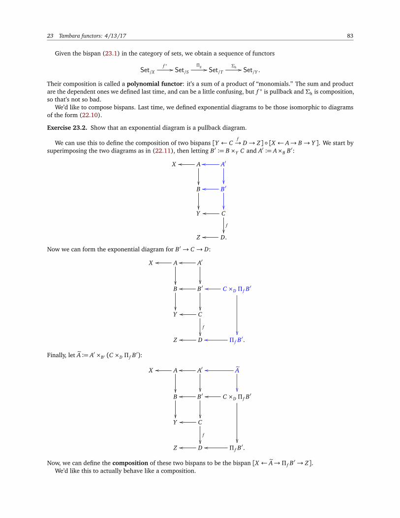
23 Tambara functors: 4/13/17 83
Given the bispan (23.1) in the category of sets, we obtain a sequence of functors
Set/Xf ∗ // Set/S
Πg // Set/TΣh // Set/Y .
Their composition is called a polynomial functor: it’s a sum of a product of “monomials.” The sum and productare the dependent ones we defined last time, and can be a little confusing, but f ∗ is pullback and Σh is composition,so that’s not so bad.
We’d like to compose bispans. Last time, we defined exponential diagrams to be those isomorphic to diagramsof the form (22.10).
Exercise 23.2. Show that an exponential diagram is a pullback diagram.
We can use this to define the composition of two bispans [Y ← Cf→ D→ Z] [X ← A→ B→ Y ]. We start by
superimposing the two diagrams as in (22.11), then letting B′ := B ×Y C and A′ := A×B B′:
X Aoo
A′oo
B
B′oo
Y Coo
f
Z D.oo
Now we can form the exponential diagram for B′→ C → D:
X Aoo
A′oo
B
B′oo
C ×D Π f B′oo
Y Coo
f
Z Doo Π f B′.oo
Finally, let eA := A′ ×B′ (C ×D Π f B′):
X Aoo
A′oo
eAoo
B
B′oo
C ×D Π f B′oo
Y Coo
f
Z Doo Π f B′.oo
Now, we can define the composition of these two bispans to be the bispan [X ← eA→ Π f B′→ Z].We’d like this to actually behave like a composition.

84 M392C (Topics in Algebraic Topology) Lecture Notes
Lemma 23.3. Composition with the identity bispan
Y Yidoo id // Y id // Y
is the identity, up to natural isomorphism.
Partial proof. Let [Xf← A
g→ B
h→ Y ] be some other bispan. Then, ΠidB ∼= B, and pulling back by the identity acts
as the identity, so B′ = B and A′ = A. Thus, Y ×Y ΠidB ∼= ΠidB = B and eA= A (again, we’re pulling back by theidentity map), so we obtain the diagram
X Afoo
g
Aidoo
g
Aidoo
g
B
h
Bidoo
h
Bidoo
Y Yidoo
id
Y Yidoo B.hoo
and therefore the composition is [X ← A→ B→ Y ] again, at least up to natural isomorphism.
Exercise 23.4. Finish the proof by checking composition with the identity on the right.
Remark. We’re working towards showing that isomorphism classes of bispans are the morphisms in a category. Ifyou don’t like taking isomorphism classes, you can use bispans on the nose, in which case you’ll get a bicategory. Ifyou like this, it’s an exercise to write this out carefully. In general, since working through this argument (at eithercategorical level) is a useful exercise, it’s not written down explicitly: if you work through this stuff, feel free toadd it to the notes.
That said, associativity is going to be a chore no matter how you go about it. (
Last time in Example 22.6, we defined three bispans R f , N f , and T f associated with a map f : S→ T .
Lemma 23.5. [Xf← A
g→ B
h→ Z] is isomorphic to the composition Th Ng R f .
Partial proof. Recall R f = [Xf← S
id→ S
id→ S] and Ng = [S
id← S
g→ T
id→ T]. We’ll show their composition is
(23.6) X Sfoo g // T id // T.
Pullbacks by the identity are the identity, so we can start with
X Sfoo
id
Sidoo
id
S
id
Sidoo
id
S Sidoo
g
T T.
idoo
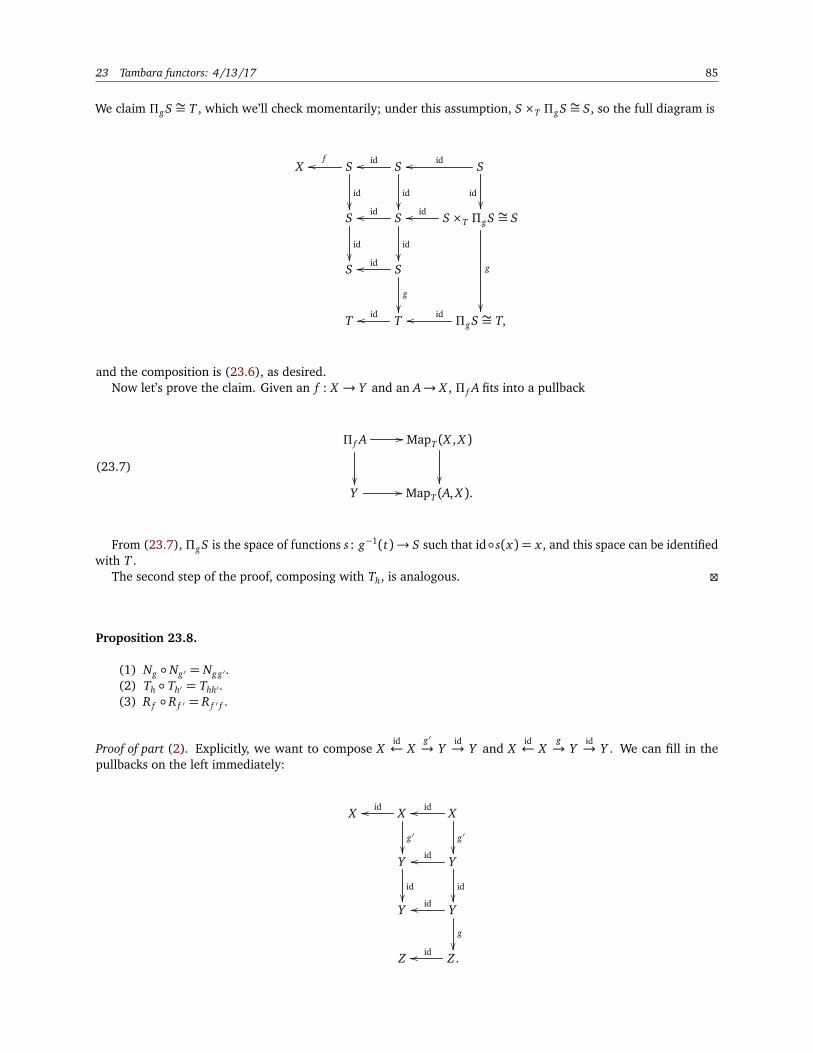
23 Tambara functors: 4/13/17 85
We claim ΠgS ∼= T , which we’ll check momentarily; under this assumption, S ×T ΠgS ∼= S, so the full diagram is
X Sfoo
id
Sidoo
id
Sidoo
id
S
id
Sidoo
id
S ×T ΠgS ∼= S
g
idoo
S Sidoo
g
T Tidoo ΠgS ∼= T,
idoo
and the composition is (23.6), as desired.Now let’s prove the claim. Given an f : X → Y and an A→ X , Π f A fits into a pullback
(23.7)
Π f A //
MapT (X , X )
Y // MapT (A, X ).
From (23.7), ΠgS is the space of functions s : g−1(t)→ S such that id s(x) = x , and this space can be identifiedwith T .
The second step of the proof, composing with Th, is analogous.
Proposition 23.8.
(1) Ng Ng ′ = Ng g ′ .(2) Th Th′ = Thh′ .(3) R f R f ′ = R f ′ f .
Proof of part (2). Explicitly, we want to compose Xid← X
g ′→ Y
id→ Y and X
id← X
g→ Y
id→ Y . We can fill in the
pullbacks on the left immediately:
X Xidoo
g ′
Xidoo
g ′
Y
id
Yidoo
id
Y Yidoo
g
Z Z .
idoo
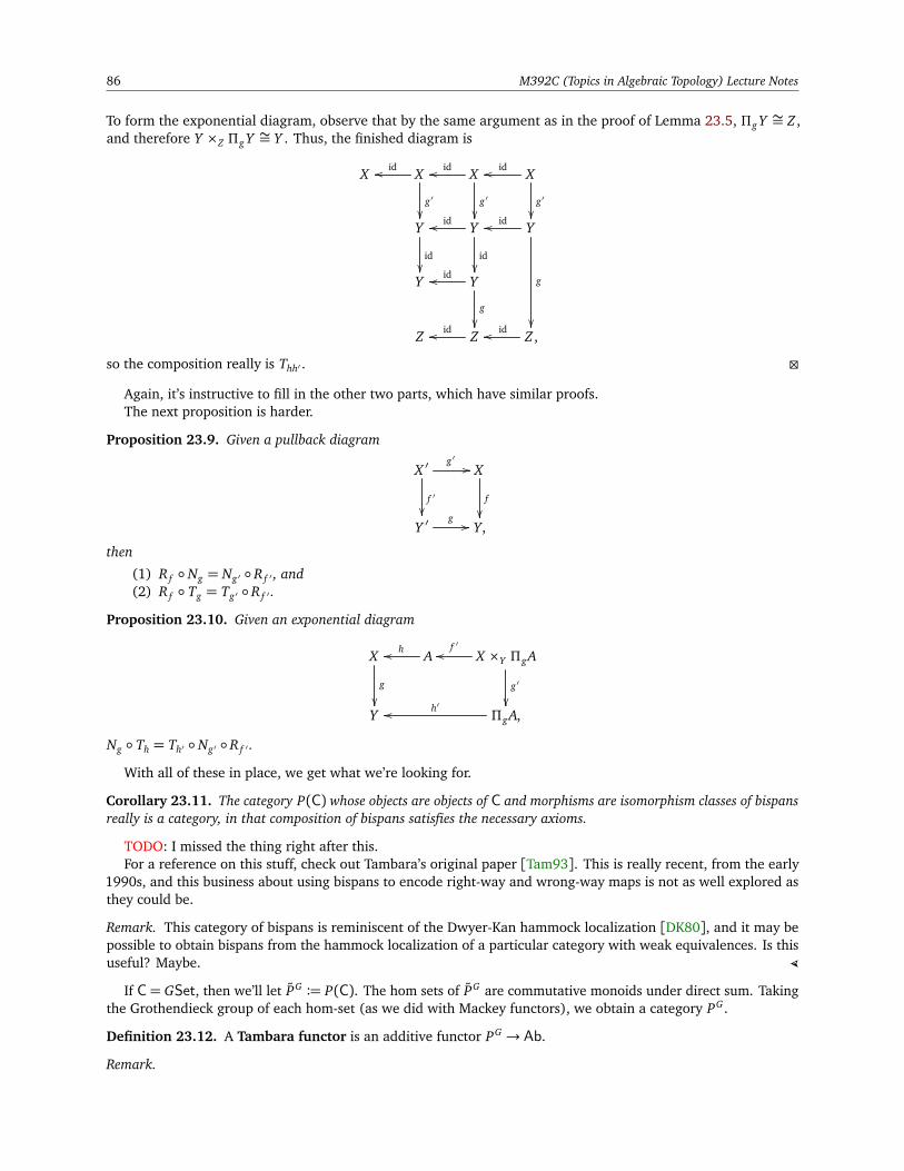
86 M392C (Topics in Algebraic Topology) Lecture Notes
To form the exponential diagram, observe that by the same argument as in the proof of Lemma 23.5, Πg Y ∼= Z ,and therefore Y ×Z Πg Y ∼= Y . Thus, the finished diagram is
X Xidoo
g ′
Xidoo
g ′
Xidoo
g ′
Y
id
Yidoo
id
Yidoo
g
Y Yidoo
g
Z Zidoo Z ,
idoo
so the composition really is Thh′ .
Again, it’s instructive to fill in the other two parts, which have similar proofs.The next proposition is harder.
Proposition 23.9. Given a pullback diagram
X ′g ′ //
f ′
X
f
Y ′
g // Y,
then
(1) R f Ng = Ng ′ R f ′ , and(2) R f Tg = Tg ′ R f ′ .
Proposition 23.10. Given an exponential diagram
X
g
Ahoo X ×Y ΠgAf ′oo
g ′
Y ΠgA,
h′oo
Ng Th = Th′ Ng ′ R f ′ .
With all of these in place, we get what we’re looking for.
Corollary 23.11. The category P(C) whose objects are objects of C and morphisms are isomorphism classes of bispansreally is a category, in that composition of bispans satisfies the necessary axioms.
TODO: I missed the thing right after this.For a reference on this stuff, check out Tambara’s original paper [Tam93]. This is really recent, from the early
1990s, and this business about using bispans to encode right-way and wrong-way maps is not as well explored asthey could be.
Remark. This category of bispans is reminiscent of the Dwyer-Kan hammock localization [DK80], and it may bepossible to obtain bispans from the hammock localization of a particular category with weak equivalences. Is thisuseful? Maybe. (
If C = GSet, then we’ll let PG := P(C). The hom sets of PG are commutative monoids under direct sum. Takingthe Grothendieck group of each hom-set (as we did with Mackey functors), we obtain a category PG .
Definition 23.12. A Tambara functor is an additive functor PG → Ab.
Remark.
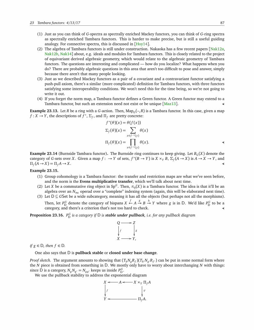
23 Tambara functors: 4/13/17 87
(1) Just as you can think of G-spectra as spectrally enriched Mackey functors, you can think of G-ring spectraas spectrally enriched Tambara functors. This is harder to make precise, but is still a useful guidinganalogy. For connective spectra, this is discussed in [Hoy14].
(2) The algebra of Tambara functors is still under construction. Nakaoka has a few recent papers [Nak12a,Nak12b, Nak14] about, e.g. ideals and modules for Tambara functors. This is closely related to the projectof equivariant derived algebraic geometry, which would relate to the algebraic geometry of Tambarafunctors. The questions are interesting and complicated — how do you localize? What happens when youdo? There are probably algebraic questions in this area that aren’t too difficult to pose and answer, simplybecause there aren’t that many people looking.
(3) Just as we described Mackey functors as a pair of a covariant and a contravariant functor satisfying apush-pull axiom, there’s a similar (more complicated) definition for Tambara functors, with three functorssatisfying some interoperability conditions. We won’t need this for the time being, so we’re not going towrite it out.
(4) If you forget the norm map, a Tambara functor defines a Green functor. A Green functor may extend to aTambara functor, but such an extension need not exist or be unique [Maz13]. (
Example 23.13. Let R be a ring with a G-action. Then, MapG(–, R) is a Tambara functor. In this case, given a mapf : X → Y , the descriptions of f ∗, Σ f , and Π f are pretty concrete:
f ∗(θ )(x) = θ ( f (x))
Σ f (θ )(x) =∑
x∈ f −1(y)
θ (x)
Π f (θ )(x) =∏
x∈ f −1(y)
θ (x). (
Example 23.14 (Burnside Tambara functor). The Burnside ring continues to keep giving. Let BG(X ) denote thecategory of G-sets over X . Given a map f : → Y of sets, f ∗(B → Y ) is X ×Y B, Σ f (A→ X ) is A→ X → Y , andΠ f (A→ X ) = Π f A→ X . (
Example 23.15.(1) Group cohomology is a Tambara functor: the transfer and restriction maps are what we’ve seen before,
and the norm is the Evens multiplicative transfer, which we’ll talk about next time.(2) Let X be a commutative ring object in SpG . Then, π0(X ) is a Tambara functor. The idea is that it’ll be an
algebra over an N∞ operad over a “complete” indexing system (again, this will be elaborated next time).(3) Let D ⊆ GSet be a wide subcategory, meaning it has all the objects (but perhaps not all the morphisms).
Then, let PGD denote the category of bispans X
f← A
g→ B
h→ Y where g is in D. We’d like PG
D to be acategory, and there’s a criterion that’s not too hard to check. (
Proposition 23.16. PGD is a category if D is stable under pullback, i.e. for any pullback diagram
Q //
f
Z
g
X // Y,
if g ∈D, then f ∈D.
One also says that D is pullback stable or closed under base change.
Proof sketch. The argument amounts to showing that (ThNgR f )(Th′Ng ′R f ′) can be put in some normal form wherethe N piece is obtained from something in D. We mostly only have to worry about interchanging N with things:since D is a category, Ng Ng ′ = Ng g ′ keeps us inside PG
D .We use the pullback stability to address the exponential diagram
X
f
Aoo X ×Y Π f A
ϕ
oo
Y Π f A.oo
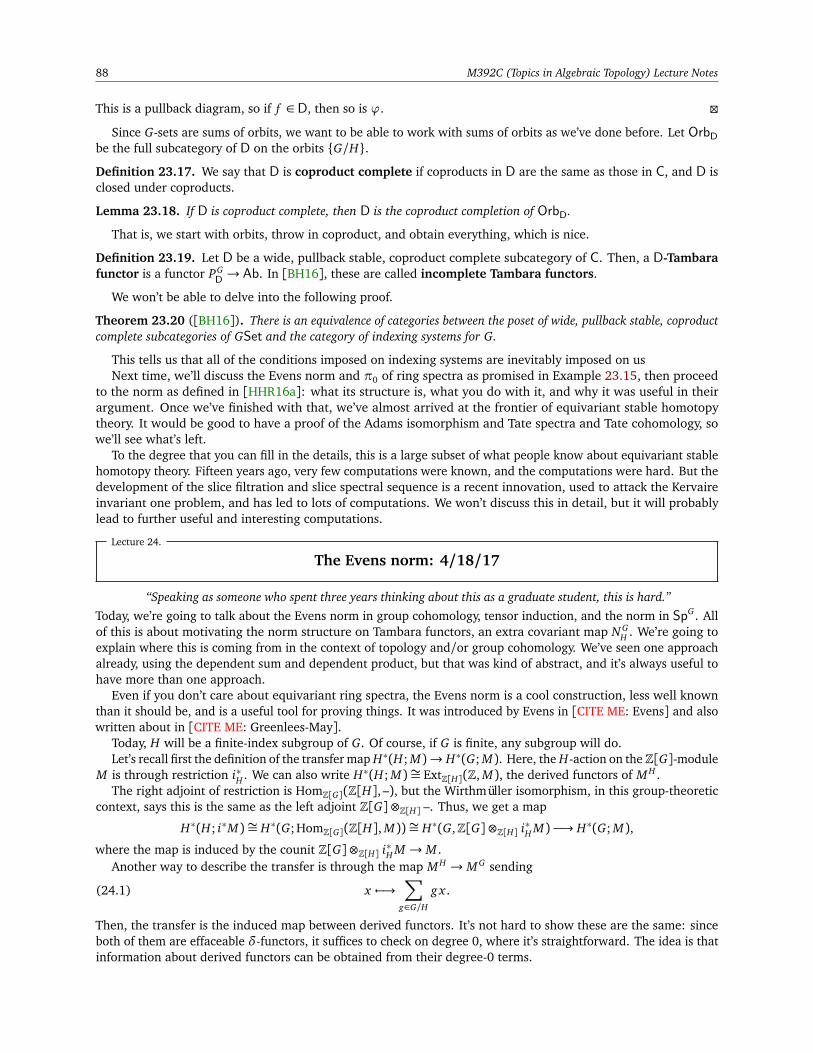
88 M392C (Topics in Algebraic Topology) Lecture Notes
This is a pullback diagram, so if f ∈D, then so is ϕ.
Since G-sets are sums of orbits, we want to be able to work with sums of orbits as we’ve done before. Let OrbDbe the full subcategory of D on the orbits G/H.
Definition 23.17. We say that D is coproduct complete if coproducts in D are the same as those in C, and D isclosed under coproducts.
Lemma 23.18. If D is coproduct complete, then D is the coproduct completion of OrbD.
That is, we start with orbits, throw in coproduct, and obtain everything, which is nice.
Definition 23.19. Let D be a wide, pullback stable, coproduct complete subcategory of C. Then, a D-Tambarafunctor is a functor PG
D → Ab. In [BH16], these are called incomplete Tambara functors.
We won’t be able to delve into the following proof.
Theorem 23.20 ([BH16]). There is an equivalence of categories between the poset of wide, pullback stable, coproductcomplete subcategories of GSet and the category of indexing systems for G.
This tells us that all of the conditions imposed on indexing systems are inevitably imposed on usNext time, we’ll discuss the Evens norm and π0 of ring spectra as promised in Example 23.15, then proceed
to the norm as defined in [HHR16a]: what its structure is, what you do with it, and why it was useful in theirargument. Once we’ve finished with that, we’ve almost arrived at the frontier of equivariant stable homotopytheory. It would be good to have a proof of the Adams isomorphism and Tate spectra and Tate cohomology, sowe’ll see what’s left.
To the degree that you can fill in the details, this is a large subset of what people know about equivariant stablehomotopy theory. Fifteen years ago, very few computations were known, and the computations were hard. But thedevelopment of the slice filtration and slice spectral sequence is a recent innovation, used to attack the Kervaireinvariant one problem, and has led to lots of computations. We won’t discuss this in detail, but it will probablylead to further useful and interesting computations.
Lecture 24.
The Evens norm: 4/18/17
“Speaking as someone who spent three years thinking about this as a graduate student, this is hard.”Today, we’re going to talk about the Evens norm in group cohomology, tensor induction, and the norm in SpG . Allof this is about motivating the norm structure on Tambara functors, an extra covariant map N G
H . We’re going toexplain where this is coming from in the context of topology and/or group cohomology. We’ve seen one approachalready, using the dependent sum and dependent product, but that was kind of abstract, and it’s always useful tohave more than one approach.
Even if you don’t care about equivariant ring spectra, the Evens norm is a cool construction, less well knownthan it should be, and is a useful tool for proving things. It was introduced by Evens in [CITE ME: Evens] and alsowritten about in [CITE ME: Greenlees-May].
Today, H will be a finite-index subgroup of G. Of course, if G is finite, any subgroup will do.Let’s recall first the definition of the transfer map H∗(H; M)→ H∗(G; M). Here, the H-action on theZ[G]-module
M is through restriction i∗H . We can also write H∗(H; M)∼= ExtZ[H](Z, M), the derived functors of M H .The right adjoint of restriction is HomZ[G](Z[H], –), but the Wirthmüller isomorphism, in this group-theoretic
context, says this is the same as the left adjoint Z[G]⊗Z[H] –. Thus, we get a map
H∗(H; i∗M)∼= H∗(G;HomZ[G](Z[H], M))∼= H∗(G,Z[G]⊗Z[H] i∗H M) −→ H∗(G; M),
where the map is induced by the counit Z[G]⊗Z[H] i∗H M → M .Another way to describe the transfer is through the map M H → M G sending
(24.1) x 7−→∑
g∈G/H
g x .
Then, the transfer is the induced map between derived functors. It’s not hard to show these are the same: sinceboth of them are effaceable δ-functors, it suffices to check on degree 0, where it’s straightforward. The idea is thatinformation about derived functors can be obtained from their degree-0 terms.
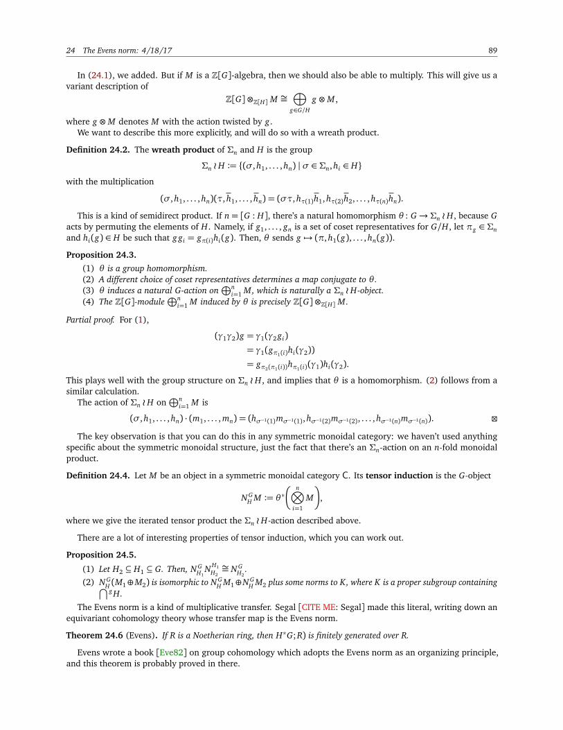
24 The Evens norm: 4/18/17 89
In (24.1), we added. But if M is a Z[G]-algebra, then we should also be able to multiply. This will give us avariant description of
Z[G]⊗Z[H] M ∼=⊕
g∈G/H
g ⊗M ,
where g ⊗M denotes M with the action twisted by g.We want to describe this more explicitly, and will do so with a wreath product.
Definition 24.2. The wreath product of Σn and H is the group
Σn oH := (σ, h1, . . . , hn) | σ ∈ Σn, hi ∈ H
with the multiplication
(σ, h1, . . . , hn)(τ, h1, . . . , hn) = (στ, hτ(1)h1, hτ(2)h2, . . . , hτ(n)hn).
This is a kind of semidirect product. If n = [G : H], there’s a natural homomorphism θ : G→ Σn oH, because Gacts by permuting the elements of H. Namely, if g1, . . . , gn is a set of coset representatives for G/H, let πg ∈ Σnand hi(g) ∈ H be such that g gi = gπ(i)hi(g). Then, θ sends g 7→ (π, h1(g), . . . , hn(g)).
Proposition 24.3.
(1) θ is a group homomorphism.(2) A different choice of coset representatives determines a map conjugate to θ .(3) θ induces a natural G-action on
⊕ni=1 M, which is naturally a Σn oH-object.
(4) The Z[G]-module⊕n
i=1 M induced by θ is precisely Z[G]⊗Z[H] M.
Partial proof. For (1),
(γ1γ2)g = γ1(γ2 gi)
= γ1(gπ1(i)hi(γ2))
= gπ2(π1(i))hπ1(i)(γ1)hi(γ2).
This plays well with the group structure on Σn o H, and implies that θ is a homomorphism. (2) follows from asimilar calculation.
The action of Σn oH on⊕n
i=1 M is
(σ, h1, . . . , hn) · (m1, . . . , mn) = (hσ−1(1)mσ−1(1), hσ−1(2)mσ−1(2), . . . , hσ−1(n)mσ−1(n)).
The key observation is that you can do this in any symmetric monoidal category: we haven’t used anythingspecific about the symmetric monoidal structure, just the fact that there’s an Σn-action on an n-fold monoidalproduct.
Definition 24.4. Let M be an object in a symmetric monoidal category C. Its tensor induction is the G-object
N GH M := θ ∗
n⊗
i=1
M
,
where we give the iterated tensor product the Σn oH-action described above.
There are a lot of interesting properties of tensor induction, which you can work out.
Proposition 24.5.
(1) Let H2 ⊆ H1 ⊆ G. Then, N GH1
N H1H2
∼= N GH2
.(2) N G
H (M1⊕M2) is isomorphic to N GH M1⊕N G
H M2 plus some norms to K, where K is a proper subgroup containing⋂
g H.
The Evens norm is a kind of multiplicative transfer. Segal [CITE ME: Segal] made this literal, writing down anequivariant cohomology theory whose transfer map is the Evens norm.
Theorem 24.6 (Evens). If R is a Noetherian ring, then H∗G; R) is finitely generated over R.
Evens wrote a book [Eve82] on group cohomology which adopts the Evens norm as an organizing principle,and this theorem is probably proved in there.
90 M392C (Topics in Algebraic Topology) Lecture Notes
Definition 24.7. The Evens norm is a map H p(H;R) → H pn(G;R) (where R is a Z[G]-algebra) which sends
α ∈ H p(H; R) to α⊗n in N GH R (with its Σn oH-action), then pulls back by θ ∗(α⊗n) to define the Evens norm of α.
We will assume α is in even degree: otherwise, there are factors (−1) to the sign of a permutation. The trick isthat instead of using the counit Z[G]⊗Z[H] i∗H M → M , we use the twisted counit
n⊗
i=1
R −→ R
coming from multiplication. The interesting piece is that this plays well with the G-action: it’s really a mapN G
H (i∗HR)→ R. In other words, it’s easy to get a map H p(H; M)→ H pn
(G; Rn), and we use the ring structure to getback to R. There’s a nice analogy of the norm as the multiplicative transfer, where we’ve replaced one counit withanother. From this perspective, the definition of an N∞-operad makes more sense.
More explicitly, let P• → R be a projective resolution of R as a Z[H]-module, so we obtain a resolutionP⊗n• → R⊗n→ R. Then, let ε : Q•→ R be a resolution of R as a Z[Σn]-object (induced from the Σn oH-action).82
We can join these into a resolution
Q• ⊗R P⊗n•
// R⊗R R⊗n // R,
and given some cocycle f : Pp → R, ε ⊗ f n is a cocycle for H pn whose cohomology class is the Evens norm of f .This is far from obvious, but comes from the fact that
(P⊗n• )np
// P⊗np
// R
produces cocycles for Hnp(H; R).83
Remark.
(1) The Evens norm satisfies a double coset formula, similarly to the transfer map.(2) The Evens norm is part of a Tambara functor structure where
G/H 7−→⊕
i=0
H2i(H; –).
(3) Multiplicative transfers, e.g. power operations, are ubiquitous, e.g. the Steenrod operations. In fact, onecan realize the Steenrod operations as a homotopical version of this norm construction, and this is afruitful approach to research for some homotopy theorists. The analogue of the twisted action is a mapEΣn ×Σn
X n→ X , which is used to construct the Steenrod operations. (
Now we want to talk about a norm map N GH : SpH → SpG . We know what we want to do, but the technicalities
are tricky.
“Definition” 24.8. The norm map N GH : SpH → SpG sends
M 7−→ θ ∗
∧
g∈G/H
M
,
which is the indexed smash product, in direct analogue with tensor induction.
The reason we use the smash product instead of the wedge sum is that spectra are already abelian groups. Theadditive analogue of this construction is the Wirthmüller isomorphism.
What makes this construction tricky is figuring out how to give∧
g∈G/H M a Σn o H-action. The issue is theuniverse.
Example 24.9. Let X ∈ Sp, and let’s consider N C2e X . If U is the universe we started with, X ∧ X is in U ⊕ U , and
the smash product is a Kan extension along U ⊕ U → U .If X is a space, C2 acts on X × X by switching the pairs. And we know the diagonal map x 7→ (x , x) defines
an isomorphism X∼=→ (N C2
e X )C2 . But if you have spectra instead, and the two universes are different, i.e. U1 ⊕ U2instead of U ⊕ U , which makes it hard to resolve. (
82Don’t we need to act on R⊕n, rather than R?83TODO: I didn’t follow this.

25 The Evens norm: 4/18/17 91
The solution is a trick, due to unpublished work of Lydakis and elucidated by [HHR16a]. Consider X in thetrivial H-universe, i.e. X is an H-object in Sp. Then there’s no problem: N C2
e X is a C2-object in Sp, or SpC2 withthe trivial universe. If we’re not keeping track of the equivariant universe, it’s easy to make sense of the mapN G
H : HSp→ GSp.The trick is the following point, which is extremely subtle: we can define N H
G : SpH → SpG by changing theuniverse from SpH to HSp (i.e. the trivial universe), then using the tensor induction to get to GSp (i.e. the trivialuniverse), then changing universe again to get back to SpG . As a point-set construction, well, sure, this is a functor.But the crazy thing is that this works: you can make this a homotopical functor such that its derived functor is theright thing.
We’ll discuss the change-of-universe map next time; this is a Kan extension along diagrams, which will makethis construction less sketchy.
Recall that SpG[P] denotes the category of commutative ring objects in G-spectra (sometimes also writtenCommH). We’ll show that N G
H : SpH[P] → SpG[P] is left adjoint to i∗H , and hence, if R is a commutative ringG-spectrum, we have a counit N G
H i∗HR→ R as we did in group cohomology.The principal player in [HHR16a] is obtained from this norm and a concrete C2-spectrum: in Definition 26.5,
we’ll define real bordism MR, the cobordism theory of stably almost complex manifolds with a C2-action by complexconjugation (there are some nuances to writing this down). Then, they consider the C8-theory N C8
C2MR, and do
a lot of hard work to show this detects the Kervaire invariant in the stable homotopy groups of spheres. Peopleare still working out the applications of this spectrum and this idea more generally, and you could count yourselfamong their numbers.
Lecture 25.
The HHR norm: 4/20/17
“Do I dare disturb the universe?”
Today, we’re going to discuss the construction and some properties of the HHR norm N GH : SpH → SpG and
N GH : SpH[P]→ SpG[P]. This is the left adjoint to i∗H (for commutative algebras), and is the basis for multiplicative
induction in the spectral setting. Thus it specializes to the norm in algebra.First, though, we’ll take a historical detour and discuss the difference between Γ -G-spaces and ΓG-spaces. This
arises from a reasonable question: what’s the analogue of a Γ -space in the equivariant context?Recall that Γ is the category of based finite sets and based maps, and the category of Γ -spaces is the functor
category Fun(Γ ,Top∗), as we discussed in Example 10.20. A special Γ -space X is the analogue of an abelian group:we ask that the induced map
X (n) −→n∏
i=1
X (1)
is an equivalence.In the equivariant setting, there are two things we can do:
• Γ -G-spaces are Γ -objects in GTop∗. These were introduced by Segal [Seg78].• Let ΓG be the category of finite based G-sets and all based maps, so it’s G-enriched, where G acts by
conjugation on the mapping space. Then, ΓG-spaces are the enriched functors ΓG → GTop∗. These wereintroduced by Shimakawa [Shi89].
Which of these is right? Turns out both are.
Theorem 25.1 (Shimakawa [Shi91]). These two categories are equivalent.
We can also line up the special conditions in a nice way. The proof uses that one weird trick in diagram spectra.The manifestation in orthogonal spectra means that the category of orthogonal spectra on the trivial universe isequivalent (on the point-set level) to orthogonal spectra on the complete universe! And in fact this is true for anyuniverse.
The reason this happens is that diagram spectra mix the point-set and homotopical data in a way that canbe confusing. Of course, the homotopy groups depend on the universe, so the homotopy theory and homotopycategory are genuinely different.

92 M392C (Topics in Algebraic Topology) Lecture Notes
Remark. You might be thinking that this is an artifact of one’s desire for concreteness and model categories, butthe∞-categorical view isn’t necessarily easier: yes, you don’t have to worry as much about point-set phenomena,and all functors are derived, but it’s a lot harder to infer the homotopy theory from first principles and you canwrite stuff down, but it’s not at all clear how to prove it’s the right thing.
To be sure, some of the difficulties in writing down the correct norm map were point-set in nature; but not allof them were. (
Since finite based sets are finite based G-sets (with G acting trivially), there is an inclusion Γ → ΓG , whichinduces a functor
R: Fun(ΓG , GTop∗) −→ Fun(Γ , GTop∗).It has a left adjoint
L : Fun(Γ , GTop∗) −→ Fun(ΓG , GTop∗),which is a Kan extension, explicitly given by the coend
LX =
∫ Γ
Hom(n, –)× X (–) =∐
n≥0
Map(n, S)× X (n)/∼,
where (s f , x)∼ (s, X ( f )x) for any Γ -morphism f : n→ m. The G-action is g[s, x] = [gs, g x].Now, L is an equivariant functor: if f : S→ T is a ΓG-morphism,
LX (g f g−1)[s, x] = [g f g−1s, x]
= g[ f g−1s, g−1 x]
= g LX ( f )[g−1s, g−1 x].
Exercise 25.2. Check that L and R are adjoint. This follows from essentially formal reasons.
Proposition 25.3. (L, R) are adjoint equivalences.
Proof. We need to check that the natural transformations id→ RL and LR→ id are natural isomorphisms. Thefirst is formal: we’re Kan extending along a full subcategory, and in this case id→ RL is always an equivalence.
Now, we want to recover X (S) from X (n), where |S|= n.84 Choose a bijection f : S→ n. The key is that thisdefines a map ρ : G→ Hom(n, n)∼= Σn, through the G-action on S. But now this looks familiar from the story ofG-operads. Why were we able to get away with indexing them on finite sets rather than on finite G-sets? Well,from the∞-categorical perspective, maybe it would be better, but we were able to get away with using just finitesets by the same trick!
So now we have a commutative diagram
Sf //
g
n
ρ(g)
S
f// n.
Endow X (n) with a new G-action85 via the map G × X (n)→ X (n) sending
g, x 7−→ X (ρ(g))(g x).
We’ll call this G-space X (n)ρ. This is another manifestation of a common principle from this class: just like finitesums and finite products are the same in the stable setting, in the equivariant stable setting, finite G-indexedsums and finite G-indexed products are the same. Since X (n) is a product of n copies of X (1), this is a G-indexedproduct.
Now, we claim that as G-spaces, X (S)∼= X (n)ρ.
Exercise 25.4. Prove this. There’s an obvious map, and you just have to check that it’s G-equivariant, like we didfor L above.
Assuming this exercise, we get that LR→ id is a natural isomorphism.
Now, what does it mean to be special in the equivariant setting?84We’re using n to denote both the set 1, . . . , n and its cardinality; hopefully they can be distinguished from context.85X (n) was already a G-space, but we’re putting a different G-action on it.

25 The HHR norm: 4/20/17 93
Definition 25.5.
• A special ΓG-space is one for which the natural map
X (S)∼=−→∏
S
X (1)
is an equivalence.• A special Γ -G-space is one for which the natural map
X (S)∼=−→
n∏
i=1
X (1)
is an equivalence86 — not just of G-spaces, but for the family of subsets H ⊂ G×Σn such that H∩(e,σ) =∅.87
The definition for Γ -G-spaces again is reminiscent to the operadic story: we’re asking for homomorphisms.
Exercise 25.6. Show that under the equivalence of Proposition 25.3, these two notions of special objects areidentified.
Remark.
(1) You can run the rest of Segal’s story: there’s a notion of a very special Γ -G-space or ΓG-space, which is acondition on fixed points, and using similar machinery as before, you can turn very special objects intoconnective genuine G-spectra.
(2) We didn’t discuss the homotopy theory of these two categories: the natural notions of fibrancy for ΓG-spacesand G-Γ -spaces are different. This is analogous to the difference between the naïve homotopy groups ofG-spectra on the trivial universe, and the more sophisticated homotopy groups that you could define onthem, and which agree with the homotopy groups of G-spectra on the complete universe. This is reallysaying something about Kan extensions and diagram spaces. (
We’re going to do some constructions with orthogonal spectra now, so let’s recall how orthogonal G-spectra aredefined, especially since we covered it rather quickly.88
Recall that if V and V ′ are real G-representations on inner product spaces, we defined IG(V, V ′) to be theG-space of linear isometries V → V ′. We defined JG(V, V ′) to be the Thom space for E ⊆ IG(V, V ′)×V ′→ IG(V, V ′),where E is the orthogonal complement
E := ( f , x) | x ∈ V − f V.
When V ⊆ V ′, you can write this explicitly as
JG(V, V ′) = O(V ′)+ ∧O(V ′−V ) SV ′−V .
Now, let JG be the category whose objects are G-representations on finite-dimensional real inner product spacesand whose morphism spaces are JG(V, V ′) as we defined them. In particular, there’s a composition law JG(V ′, V ′′)×JG(V, V ′)→ JG(V, V ′′) and a symmetric monodial product
( f , x) + ( f ′, x ′) = ( f + f ′, x + x ′)
(g, y)( f , x) = (g f , g x + y).
The unit is (id, 0).Now, we were able to define SpG = Fun(JG , GTop∗), and we saw this has a symmetric monoidal structure.One important point is that the Yoneda lemma implies
(25.7)∨
V,W
S−W ∧ JG(V, W )∧ X (V ) // //∨
V
S−V ∧ X (V ) // X
is a coequalizer of X in terms of representable objects. This is true in general for presheaves, and in thiscontext, [HHR16a] call it the tautological presentation of X .
86TODO: I might have gotten this criterion wrong.87This is what Segal missed.88TODO: there may be notational inconsistencies with the first time orthogonal spectra were covered, which I should fix at some point.

94 M392C (Topics in Algebraic Topology) Lecture Notes
Now we’ll introduce the point-set change-of-universe functor SpG[U ′] → SpG[U], where U and U ′ are G-universes. Let
IUU ′X (V ) := JG(Rn, V )∧O(n) X (Rn),
where dim V = n. If W is a p-dimensional G-representation, the action of JG(V, W ) on this comes through thediagram
JG(V, W )∧ JG(Rn, V )∧O(n) X (Rn)
JG(Rn, W )∧O(n) X (Rn) // JG(Rp, W )∧O(p) J ′G(R
n,Rp)∧O(n) X (Rn) // JG(Rp, W )∧O(p) X (Rp).
Exercise 25.8. Show that IUU ′ I
U ′U = id. This is not hard. Also, check that IU
U ′ is strong symmetric monoidal.
Thus, for any U and U ′, SpG[U] and SpG[U ′] are equivalent! This is true for the same reason as Proposition 25.3.
Remark. It’s also quick to check that IR∞
U is the forgetful functor. (
Let U be a complete H-universe and eU be a complete G-universe. Then, we’ll define N GH : SpH
U → SpGeU
by
X 7−→ I eUR∞θ∗
∧
G/H
X
IR∞
U X .
Here θ is the wreath action we introduced last time. This functor is clearly strong symmetric monoidal, and turnsout to be left-adjoint to i∗H : SpG
eU[P]→ SpH
U [P], i.e. on the categories of commutative algebras.The miracle is that this can be derived in the usual model structure by cofibrant replacement, so it’s homotopically
the right thing. We won’t prove this; it’s one of the technically hardest parts of [HHR16a]: it’s not a left adjoint onmodules, so it doesn’t commute with colimits, and one has to carefully analyze what it does to pushouts.
There are a few key facts:
• N GH is symmetric monoidal.
• N GH S−V = S− IndG
H V .• There’s a diagonal map ΦH X → ΦGN G
H X , and it’s an equivalence. In fact, when X is cofibrant, this is apoint-set equivalence!
We’ll begin showing this by describing ΦG , which is a strong symmetric monoidal functor such that if Z is a space,ΦG(S−V ∧ Z) ∼= S−V G
∧ ZG . In the ∞-categorical sense, it commutes with colimits, but this is not true in thepoint-set case; in any case, mirroring the tautological presentation (25.7), ΦGX is the coequalizer
∨
V,W
S−W G∧ JG(V, W )G ∧ X (V )G // //
∨
V
S−V G∧ X (V )G // ΦGX .
It’s not too hard to check this is the same as the model described in [CITE ME: Mandell-May]. We’ll use thisdescription to construct the diagonal map. Using the fact that ZH ∼= (N G
H Z)G ,
ΦGN GH S−V ∼= ΦG
S− IndGH V
∼= S−V H ∼= ΦHS−V .
Therefore we have an isomorphism
ΦH(S−V ∧ Z)∼=−→ ΦGN G
H (S−V ∧ Z).
Applying this termwise to the tautological construction, we obtain a map
∨
V,W
S−W H∧ IH(V, W )G ∧ X (V )H ////
∨
V
S−V GH ∧ X (V )H // ΦGN G
H X ,
hence by the universal property of the coequalizer, a map ΦH G→ ΦGN GH X .
26 The HHR norm: 4/20/17 95
Lecture 26.
Consequences of the construction of the norm map: 4/25/17
“The genuine equivariant model is always the most painful of the two options.”Today we’re going to talk about some applications of the norm map, including why π0 of an E∞-ring spectrum is aTambara functor and how the norm construction interacts with the resolution of the Kervaire invariant 1 problem.In the next two classes we’ll talk about the Tate construction and the Tate spectral sequence; the last class is moreopen, and we can talk about current directions in research or anything else.
Over the summer, there will be more work on the notes: if you did any exercises while working this materialout, feel free to include them, even if they’re very rough. If anything is unclear or not useful or you have any othercomments, feel free to leave them in the notes.
Today, R will be a commutative ring in orthogonal G-spectra, i.e. an object of SpG[P]. The forgetful functorfrom G-ring spectra to H-ring spectra is lax symmetric monoidal and has a left adjoint, which is the HHR norm;it was known that this left adjoint existed for a long time, and that it wasn’t the same adjoint as for G-spectrawithout a ring structure, but it wasn’t understood how to think of it until recently.
One consequence is the existence of the counit η: N GH i∗HR→ R. If X ∈ SpH , then R0
H(X ) = [X , i∗HR]H , so thenorm provides us with a map R0
H(X ) → R0G(N
HG X ): given a map f : X → i∗HR, norm it and apply the counit:
ε N GH ( f ): N G
H X → N GH i∗HR→ R. This and a few similar constructions are reminiscent of the Evens norm: if V is an
H-representation and X = SV , this is a map R0H(S
V )→ R0G(N
GH SV ) = R0
G(SIndG
H V ), and these are homotopy groups:R0
H(SV ) = [SV , i∗HR] = πV (i∗HR), so we obtain a map πV (i∗HR)→ πIndG
H V (R).For example, if A is a G-space, given a map f : Σ∞A→ i∗HR, we can construct a map R0
H(i∗HA)→ R0
G(A) sendingΣ∞A→ Σ∞N G
H A, which is homeomorphic to N GHΣ
∞A (here this is the norm map on spaces); then, using f , mapto N G
H i∗HR then to R by the counit.
Exercise 26.1. This is nearly saying that π0R= R0(–) is a Tambara functor; check that this is really the case.
There’s lots of things to check: figuring out why the double coset formula holds is work, though not tooconceptually hard if you’ve followed everything so far. The original papers are complicated, because this check isinevitably notation-heavy.
On the other hand, there’s a converse:
Theorem 26.2 (Ullman [Ull12]). All Tambara functors arise as π0R for some ring spectrum R, e.g. an Eilenberg-MacLane spectrum. However, there is no Eilenberg-Mac Lane functor that is symmetric monoidal.
Remark. There’s a cool connection between the structures of Tambara functors and Witt vectors. For example,[CITE ME: Hesselholt-Madsen] identify π0THH and π0THHCpn with certain rings of Witt vectors. This fits into abigger picture. (
N∞-operads come back. We used them to specify which transfer maps you have, and here they will controlwhich norm maps you get. There are some complicated questions here: distributivity of norm and transfer maps isintricate, and the interactions between two different N∞-operads, neither of which is complete, is not writtendown.
The rough idea is that any commutative G-ring spectrum should be characterized by having certain norm mapsN G
H i∗H X → X .
Lemma 26.3. Let T be an admissible H-set for an N∞-operad O. Then,
(G ×Σ|T |/ΓT )+ ∧Σ|T | X|T | ∼= G+ ∧H
∧
i
N HKi
i∗KiX .
The idea is that we can write T as a coproduct of orbits H/Ki .Using this lemma, since T is admissible, we get a map G×Σ|T |/Γ|T |→ O(|T |), and therefore if X is an O-algebra
(i.e. is in SpG[O]), this becomes a map
G+ ∧H
∧
N HKi
i∗KiX // O(|T |)∧Σ|T | X
|T | // X ,
so for X an N∞-algebra over O, N GH : SpH[O] SpG[O] : i∗H is homotopical whenever G/H is admissible. In this
case, π0X is an incomplete Tambara functor: we asked for it to contain the norm maps for O, and we have toaccept certain other ones.
96 M392C (Topics in Algebraic Topology) Lecture Notes
If instead A is an N∞-algebra in G-spaces, then Σ∞+ A is an N∞-algebra in SpG , and is in fact the spectral groupring (also denoted S[A]). The multiplication comes from the isomorphism
O(n)×Σn(Σ∞+ A)n ∼= Σ∞+ (O(n)×Σn
An).
Remark. The nonequivariant analogue of this is called the spherical group ring of a space M , S[ΩM] := Σ∞+ ΩM .It’s worth thinking about the similarities between these two cases. (
What ends up happening is that Σ∞+ takes transfers to norms, which is a good slogan to remember.We can also look at what happens to the units of a commutative ring spectrum. Nonequivariantly, let R be a
commutative ring spectrum. Its group of units was initially defined as the space GL1R that fits into the pullbackdiagram
(26.4)
GL1Rù
//
Ω∞R
(π0Ω
∞R)× // π0Ω∞R.
This definition makes sense for any A∞-ring spectrum, but behaves better when R is commutative.
Fact.(1) If R is an E∞-ring spectrum, then GL1R is an E∞-space, and therefore extends to a spectrum called gl1R.(2) GL1 is (homotopically) the right adjoint to Σ∞+ . (
This relates to the theory of orientations, and in fact this was originally considered for this purpose by DennisSullivan, and expanded on by [May77]. The modern approach was written down in [ABG+14a, ABG+14b]. PeterMay has three articles [May09a, May09b, May09c] from the 2009 Banff conference about these things that areparticularly clear.
Another characterization of GL1R is as the homotopy automorphisms of R in the category of R-modules:GL1R= LAutModR
(R).Anyways, there’s an analogous construction in the equivariant setting [CITE ME: ???], where you have to work
out (26.4) for all fixed points simultaneously. But this works out, and you can show that GL1 sends norms totransfers, which makes sense.
An outline of the Kervaire invariant 1 proof. Of course, this is the proof in [HHR16a]. Kervaire [Ker60]connected his invariant to the stable homotopy groups of spheres, and therefore was able to show that every10-dimensional smooth manifold has Kervaire invariant zero, then produced a PL manifold with Kervaire manifold1 (hence a nonsmoothable manifold).
Browder [Bro69] managed to connect this to elements θ j ∈ πs2 j+1−2(S), so that a manifold of Kervaire invariant
one exists in a certain dimension iff there’s a differential in the Adams spectral sequence showing that θ j 6= 0.The proof idea was concocted by Ravenel in the 1970s, but the tools to implement it weren’t available until
very recently. The idea is to construct a designer cohomology theory Ω meeting the following criteria.(1) Ω is multiplicative, therefore admitting a map S→ Ω such that the image of θ j is nonzero.(2) The homotopy groups πiΩ are zero in degrees 0< i < 4.(3) π∗Ω∼= π∗+256Ω.
These suffice: the idea is that for j ≥ 7, θ j is detected by Ω, but lands in degree between 0 and 4 mod 256, somust be zero.
Remark. For a while, people suspected there were infinitely many dimensions in which manifolds with Kervaireinvariant 1 existed, which would have simplified a lot of Adams spectral sequence calculations. One manifestationof this was Cohen’s “doomsday conjecture” [Mil71], which Mahowald [Mah77] showed was false. (
Then, Hill, Hopkins, and Ravenel constructed Ω as N C8C2
MR[κ−1]: take real bordism, norm it up from C2 to C8,and then invert something (an analogue of the Bott element), and they showed it meets the desired criteria.
Definition 26.5 (Real cobordism). Real cobordism MR is a C2-spectrum originally defined by Landweber [Lan67].We’ll provide a construction for it as an orthogonal C2-spectrum due to Schwede [Sch16].
Consider the spaceMUn := EU(n)+ ∧U(n) S
Cn,
27 Consequences of the construction of the norm map: 4/25/17 97
where U(n) is the group of unitary matrices. Then, MUn is a C2-space, where the action is by complex conjugation.89
We’ll use these spaces to define a C2-ring spectrum. First, the decomposition Cn+m ∼= Cn ⊕ Cm inducesa multiplication map MUn ∧ MUm −→ MUn+m, and the map U(n) → B(U(n), U(n),∗) defines a map SC
n→
EU(n)×U(n) SCn
; together, these define C2-equivariant structure maps SCn∧MUm→MUn+m.
This is very close to the definition of an orthogonal ring spectrum, but indexed on complex representationsrather than real ones. One of the lessons of this class is that the diagram you index spectra by doesn’t matter allthat much, and there’s a way to turn these unitary spectra into orthogonal ones.
Namely, using the decomposition C= R⊕ iR, we can define
MRn :=Map(iRn, MUn),
where On and C2 both act by conjugation. The structure maps for MUn factor as
Sn ∧ S iRn∧MUk −→MUn+k,
where C2 acts on Rn by the sign representation and on MUN by complex conjugation.Now, we get an object MR ∈ SpC2 called real cobordism.
MRV :=Map(S iV , EU(VC)+ ∧U(V (C)) SVC),
where VC := V ⊗R C.
Real cobordism relates to usual cobordism spectra in nice ways: the geometric fixed points ΦC2MR∼=MO, andi∗C2
MR=MU.From here, one uses spectral sequences to compute that Ω satisfies the various criteria, including the homotopy
fixed point spectral sequence and the slice spectral sequence (which we’ll discuss in Theorem 29.5 and (28.3),respectively).
Lecture 27.
Tate spectra: 4/27/17
Today (and possibly next lecture): Tate spectra. Next week, we’ll talk about the slice spectral sequence andfuture research directions.
Tate spectra are the spectral analogue of Tate cohomology in group cohomology. This is yet another instance ofa fruitful phenomenon: group cohomology is an important source of inspiration in equivariant homotopy theory.By looking at group cohomology in the right way, we found Mackey functors, the Wirthmüller isomorphism,norms, Tambara functors, and more (though some of these were hard to see from group cohomology first). Groupcohomology is a nice testing ground, because of its concreteness: there are elements and you can add and multiplythings!
Remark. The definitive reference on Tate spectra is Greenlees-May [GM95b], which builds on [ACD89]. Thelatter is lower-tech, but is more direct and has nice ideas. Another good reference is [HM03, §4], a section ofHesselholt-Madsen’s paper about the algebraic K-theory of local fields.
The reason you can find Tate spectra in an a priori unrelated paper is that they are important for computingalgebraic K-theory via trace methods: it’s possible to compute algebraic K-theory from topological cyclic homologyand topological Hochschild homology, and the computation passes through iterated Tate spectral sequences. Thebest examples for the use of Tate spectra were until quite recently from the literature on trace methods, e.g. almostall of Hesselholt-Madsen’s papers.
There’s also a connection between Tate spectra and chromatic homotopy theory: like the redshift conjectureasserts that algebraic K-theory raises chromatic height, Tate spectra seem to have blueshift, lowering by a chromaticlevel. (
Let M be a k[G]-module. Then, the algebraic orbits are MG := k⊗k[G] M , and the algebraic fixed points areM G := Homk[G](k, M). We’ll define a map N : MG → M G , which is called a norm map, but it’s more like a transfermap. Namely, there’s a distinguished element in k[G], NG :=
∑
g∈G g, and N is multiplication by NG:
N : x 7−→∑
g∈G
g x .
89Here, EU(n) = B(U(n), U(n),∗) is a contractible space with a free U(n)-action, and the quotient is BU(n) = B(∗, U(n),∗).

98 M392C (Topics in Algebraic Topology) Lecture Notes
This lands in M , but is clearly a fixed point.
Exercise 27.1. Show that this is independent of the choice of representative for x ∈ MG .
This is slightly less obvious, but not hard.We’ll think of N as a map H0(G; M)→ H0(G; M), which “sews together” group homology and group cohomology
with coefficients in M . Nonetheless, it’s an interesting object in its own right. What we’ll get is
(27.2a) ÒH i(G; M) =
¨
H i(G; M), i ≥ 1
H−i−1(G; M), i ≤ −2,
and for i = 0, 1 there’s an exact sequence
(27.2b) 0 //ÒH−1(G; M) // H0(G; M) N // H0(G; M) //
ÒH0(G; M) // 0.
You can build this by forming complete resolutions: beginning with a pair P∗ → k and k → I∗, respectively aprojective and an injective resolution of k as a k[G]-module, and you can sew these together by truncating I∗ anddualizing to k→ P∗, then connecting them along k.90
Another construction is to let eP∗ be the mapping cone of a projective resolution P∗→ k of k as a k[G]-module.This extends to a sequence
P∗ // k //eP∗ // ΣP∗ // · · ·
Definition 27.3. Using this, define the Tate cohomology ÒH∗(G; M) is the cohomology of the complex
(eP∗ ⊗Hom(P∗, M))G .
To see that this agrees with (27.2a) and (27.2b), use the long exact sequence and a comparison
(P∗ ⊗Hom(P∗, M))G ∼= (P∗ ⊗M)G ∼= (P∗ ⊗M)G .
We’d like to imitate this construction topologically. The analogue of the projective resolution of k is EG+ → S0
which collapses everything to the non-basepoint. Let ÝEG be the cofiber of this map. Thus we get a map
X ∼= F(S0, X ) −→ F(EG+, X ),
and thus obtain a diagram of cofiber sequences:
(27.4)
EG+ ∧ X //
X
//ÝEG ∧ X
EG+ ∧ F(EG+, X ) // F(EG+, X ) //
ÝEG ∧ F(EG+, X ).
Using the Adams isomorphism,91 you can check that
(EG+ ∧ X )G ∼= XhG .
Now, apply (–)G to (27.4), and you obtain
(27.5)
XhG//
∼=
X G
ù
// ΦGX
XhG
N // X hG // X tG .
The map N is the canonical orbits-to-fixed-points map. The spectrum in the lower right, X tG , is called the Tatespectrum of X .
Remark.
90TODO: make precise.91We haven’t discussed the Adams isomorphism in this class, but you can also show this directly: the idea is that smashing with EG+ makes
things free, hence you just have to check on underlying spaces, and taking F(EG+, –) makes it cofree, so you can work with that.

27 Tate spectra: 4/27/17 99
(1) The fact that the right-hand square is a pullback diagram means that you can recover X G from ΦGX . Forexample, if G = Cp, so there’s only one nontrivial subgroup, you can describe the homotopy theory ofG-spectra diagramatically, since geometric fixed points capture weak equivalences. This philosophy is putto work in Saul Glassman’s papers.
(2) The right-hand square looks like an arithmetic square or fracture square, and this is a perspective worthtaking seriously. (
Definition 27.6. The free homotopy type or Borel homotopy type of a G-spectrum X is the homotopy type ofEG+ ∧ X .92
If you make the action free, you lose some information, but often enough remains to be useful. In particular,the bottom row of (27.5) is a cofiber sequence, so X tG only depends on the free homotopy type of X .
Remark. Since EG+ is a space, it has a diagonal, and (EG × EG)+ ∼= EG+, so it’s a ring, and therefore (–)tG is laxmonoidal. It’s a bit of a chore to make this precise.
The Tate spectrum construction is not functorial in G; however, it does define a Mackey functor [GM95b]. (
This construction now leads to the Tate spectral sequence.93 The filtrations on ÝEG and EG combine to producta filtration on ÝEG ∧ F(EG+, X ).94 Namely, let Er be a CW filtration of EG and eEr be a CW filtration of ÝEG. Let
X r,s := eEr ∧ F(E/E−s−1, X )
X r,s := hocolim0≤x≤r0≤y≤s
X x ,y
X t :=⋃
r+s=tX r,s.
Definition 27.7. The Tate spectral sequence is the spectral sequence induced from X t. It is a conditionallyconvergent spectral sequence
E2s,t = ÒH
s(G;πt X ) =⇒ πs+t XtG .
Remark. Conditionally convergent spectral sequences may be somewhat unfamiliar, and are less well behaved.Boardman’s “Conditionally convergent spectral sequences” [Boa99] is a great paper separating the informationof a spectral sequence into a structural piece and a calculational piece (using homotopy limits). Conditionalconvergence means the structural part exists. Boardman also proves a spectral sequence comparison theorem forconditionally convergent spectral sequences! Hesselholt-Madsen [HM92] make heavy use of a nonconvergentspectral sequence to make calculations about the S1-Tate spectrum of the image-of-J spectrum, which is a reallyinteresting use of nonconvergence. Their papers in general are a masterclass in thinking with spectral sequences,and this one is particularly accessible. (
The Tate spectral sequence has a relationship to the homotopy fixed-point spectral sequence, which you mightexpect.
There’s an alternate construction of the Tate spectral sequence using the Greenlees filtration of ÝEG:
E′r :=
¨
Er , r ≥ 0
DEr , r ≤ 0.
(Here, DEr =Map(Er ,S).) Then, you can smash using E′r instead of Er , and this was Greenlees’ original constructionof the Tate spectral sequence.
Let’s analyze the E1 term a bit more. There’s an isomorphism
X r/X r−1∼=∨
sWr,s,
92Borel homotopy types capture the naïve notion of equivariant spectra, namely spectra with a G-action or spectra over BG. They havesome nice properties, e.g. their homotopy fixed points are the same as their ordinary fixed points [MNN17, Prop. 6.19], and are often usefuloutside homotopy theory, such as in [FH16].
93In this argument, we’ll make nice (co)fibrancy assumptions, e.g. that X is fibrant and EG+ is cofibrant; a careful treatment would makethe (co)fibrant replacements explicit.
94One unpleasant aspect of this construction is that, though these filtrations are both cellular, and the maps in (27.4) can be made cellular.But if you do this, it’s extremely hard to see the multiplicative structure. Ongoing work of [CITE ME: Blumberg-Mandell] is trying to resolvethis.
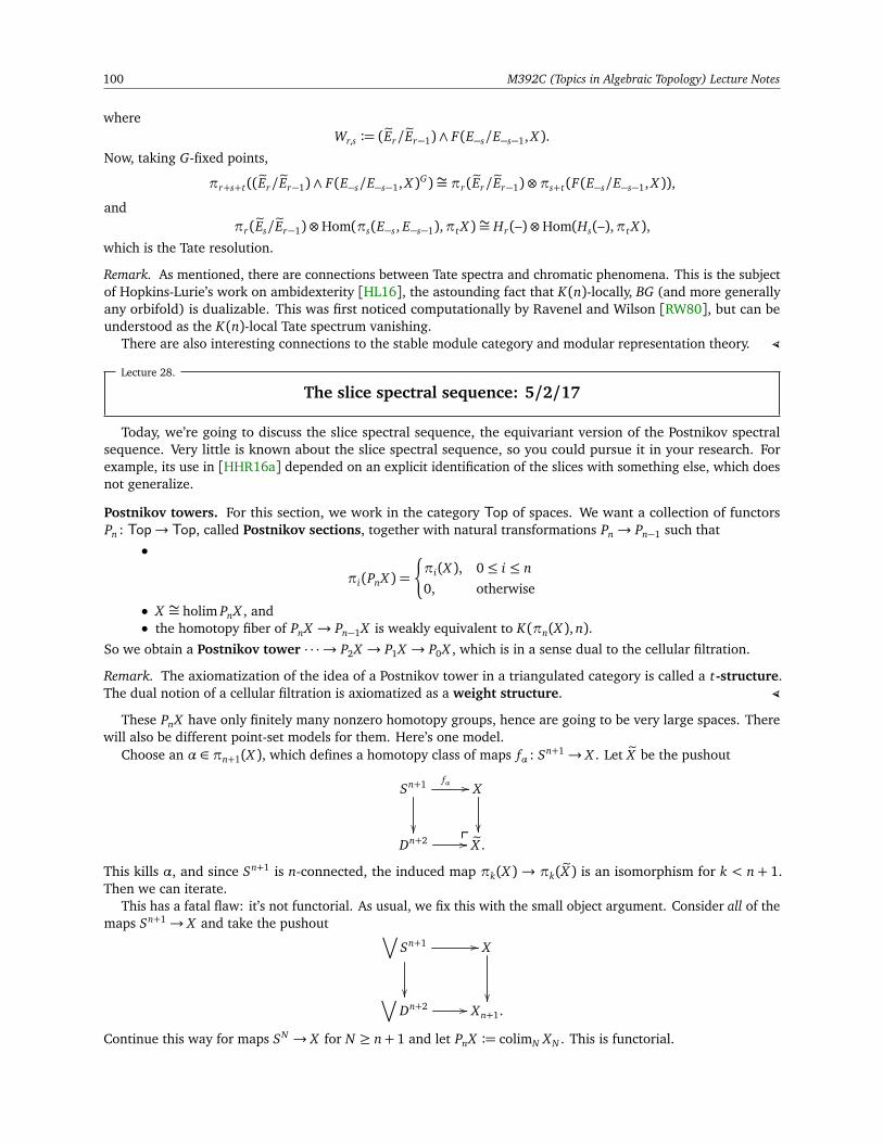
100 M392C (Topics in Algebraic Topology) Lecture Notes
whereWr,s := (eEr/eEr−1)∧ F(E−s/E−s−1, X ).
Now, taking G-fixed points,
πr+s+t((eEr/eEr−1)∧ F(E−s/E−s−1, X )G)∼= πr(eEr/eEr−1)⊗πs+t(F(E−s/E−s−1, X )),
andπr(eEs/eEr−1)⊗Hom(πs(E−s, E−s−1),πt X )∼= Hr(–)⊗Hom(Hs(–),πt X ),
which is the Tate resolution.
Remark. As mentioned, there are connections between Tate spectra and chromatic phenomena. This is the subjectof Hopkins-Lurie’s work on ambidexterity [HL16], the astounding fact that K(n)-locally, BG (and more generallyany orbifold) is dualizable. This was first noticed computationally by Ravenel and Wilson [RW80], but can beunderstood as the K(n)-local Tate spectrum vanishing.
There are also interesting connections to the stable module category and modular representation theory. (
Lecture 28.
The slice spectral sequence: 5/2/17
Today, we’re going to discuss the slice spectral sequence, the equivariant version of the Postnikov spectralsequence. Very little is known about the slice spectral sequence, so you could pursue it in your research. Forexample, its use in [HHR16a] depended on an explicit identification of the slices with something else, which doesnot generalize.
Postnikov towers. For this section, we work in the category Top of spaces. We want a collection of functorsPn : Top→ Top, called Postnikov sections, together with natural transformations Pn→ Pn−1 such that
•
πi(PnX ) =
¨
πi(X ), 0≤ i ≤ n0, otherwise
• X ∼= holim PnX , and• the homotopy fiber of PnX → Pn−1X is weakly equivalent to K(πn(X ), n).
So we obtain a Postnikov tower · · · → P2X → P1X → P0X , which is in a sense dual to the cellular filtration.
Remark. The axiomatization of the idea of a Postnikov tower in a triangulated category is called a t-structure.The dual notion of a cellular filtration is axiomatized as a weight structure. (
These PnX have only finitely many nonzero homotopy groups, hence are going to be very large spaces. Therewill also be different point-set models for them. Here’s one model.
Choose an α ∈ πn+1(X ), which defines a homotopy class of maps fα : Sn+1→ X . Let eX be the pushout
Sn+1 fα //
X
Dn+2 //
eX .ð
This kills α, and since Sn+1 is n-connected, the induced map πk(X )→ πk(eX ) is an isomorphism for k < n+ 1.Then we can iterate.
This has a fatal flaw: it’s not functorial. As usual, we fix this with the small object argument. Consider all of themaps Sn+1→ X and take the pushout
∨
Sn+1 //
X
∨
Dn+2 // Xn+1.
Continue this way for maps SN → X for N ≥ n+ 1 and let PnX := colimN XN . This is functorial.
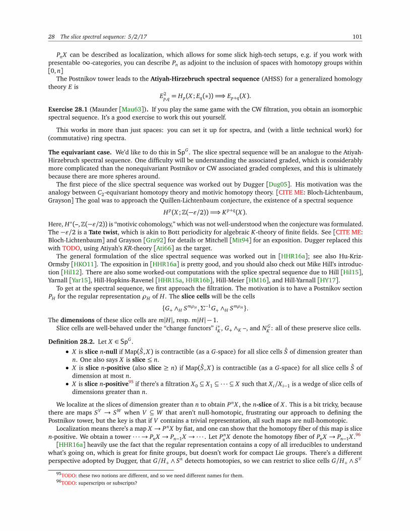
28 The slice spectral sequence: 5/2/17 101
PnX can be described as localization, which allows for some slick high-tech setups, e.g. if you work withpresentable∞-categories, you can describe Pn as adjoint to the inclusion of spaces with homotopy groups within[0, n]
The Postnikov tower leads to the Atiyah-Hirzebruch spectral sequence (AHSS) for a generalized homologytheory E is
E2p,q = Hp(X ; Eq(∗)) =⇒ Ep+q(X ).
Exercise 28.1 (Maunder [Mau63]). If you play the same game with the CW filtration, you obtain an isomorphicspectral sequence. It’s a good exercise to work this out yourself.
This works in more than just spaces: you can set it up for spectra, and (with a little technical work) for(commutative) ring spectra.
The equivariant case. We’d like to do this in SpG . The slice spectral sequence will be an analogue to the Atiyah-Hirzebruch spectral sequence. One difficulty will be understanding the associated graded, which is considerablymore complicated than the nonequivariant Postnikov or CW associated graded complexes, and this is ultimatelybecause there are more spheres around.
The first piece of the slice spectral sequence was worked out by Dugger [Dug05]. His motivation was theanalogy between C2-equivariant homotopy theory and motivic homotopy theory. [CITE ME: Bloch-Lichtenbaum,Grayson] The goal was to approach the Quillen-Lichtenbaum conjecture, the existence of a spectral sequence
H p(X ;Z(−ε/2)) =⇒ K p+q(X ).
Here, H∗(–,Z(−ε/2)) is “motivic cohomology,” which was not well-understood when the conjecture was formulated.The −ε/2 is a Tate twist, which is akin to Bott periodicity for algebraic K-theory of finite fields. See [CITE ME:Bloch-Lichtenbaum] and Grayson [Gra92] for details or Mitchell [Mit94] for an exposition. Dugger replaced thiswith TODO, using Atiyah’s KR-theory [Ati66] as the target.
The general formulation of the slice spectral sequence was worked out in [HHR16a]; see also Hu-Kriz-Ormsby [HKO11]. The exposition in [HHR16a] is pretty good, and you should also check out Mike Hill’s introduc-tion [Hil12]. There are also some worked-out computations with the splice spectral sequence due to Hill [Hil15],Yarnall [Yar15], Hill-Hopkins-Ravenel [HHR15a, HHR16b], Hill-Meier [HM16], and Hill-Yarnall [HY17].
To get at the spectral sequence, we first approach the filtration. The motivation is to have a Postnikov sectionPH for the regular representation ρH of H. The slice cells will be the cells
G+ ∧H SmρH ,Σ−1G+ ∧H SmρH .
The dimensions of these slice cells are m|H|, resp. m|H| − 1.Slice cells are well-behaved under the “change functors” i∗K , G+ ∧K –, and N G
K : all of these preserve slice cells.
Definition 28.2. Let X ∈ SpG .
• X is slice n-null if Map(S, X ) is contractible (as a G-space) for all slice cells S of dimension greater thann. One also says X is slice ≤ n.
• X is slice n-positive (also slice ≥ n) if Map(S, X ) is contractible (as a G-space) for all slice cells S ofdimension at most n.
• X is slice n-positive95 if there’s a filtration X0 ⊆ X1 ⊆ · · · ⊆ X such that X i/X i−1 is a wedge of slice cells ofdimensions greater than n.
We localize at the slices of dimension greater than n to obtain PnX , the n-slice of X . This is a bit tricky, becausethere are maps SV → SW when V ⊆ W that aren’t null-homotopic, frustrating our approach to defining thePostnikov tower, but the key is that if V contains a trivial representation, all such maps are null-homotopic.
Localization means there’s a map X → PnX by fiat, and one can show that the homotopy fiber of this map is slicen-positive. We obtain a tower · · · → PnX → Pn−1X → ·· · . Let Pn
n X denote the homotopy fiber of PnX → Pn−1X .96
[HHR16a] heavily use the fact that the regular representation contains a copy of all irreducibles to understandwhat’s going on, which is great for finite groups, but doesn’t work for compact Lie groups. There’s a differentperspective adopted by Dugger, that G/H+ ∧ Sn detects homotopies, so we can restrict to slice cells G/H+ ∧ SV
95TODO: these two notions are different, and so we need different names for them.96TODO: superscripts or subscripts?
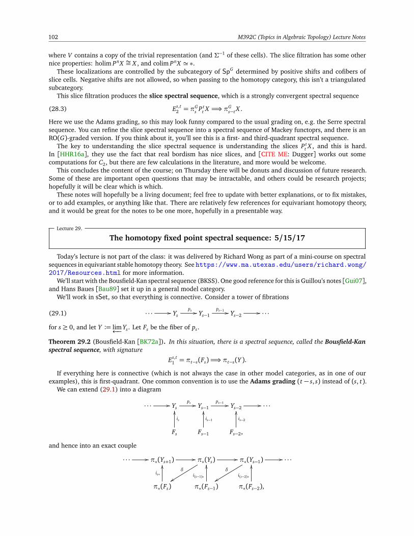
102 M392C (Topics in Algebraic Topology) Lecture Notes
where V contains a copy of the trivial representation (and Σ−1 of these cells). The slice filtration has some othernice properties: holim PnX ∼= X , and colim PnX ' ∗.
These localizations are controlled by the subcategory of SpG determined by positive shifts and cofibers ofslice cells. Negative shifts are not allowed, so when passing to the homotopy category, this isn’t a triangulatedsubcategory.
This slice filtration produces the slice spectral sequence, which is a strongly convergent spectral sequence
(28.3) Es,t2 = π
Gs P t
t X =⇒ πGs−t X .
Here we use the Adams grading, so this may look funny compared to the usual grading on, e.g. the Serre spectralsequence. You can refine the slice spectral sequence into a spectral sequence of Mackey functoprs, and there is anRO(G)-graded version. If you think about it, you’ll see this is a first- and third-quadrant spectral sequence.
The key to understanding the slice spectral sequence is understanding the slices P tt X , and this is hard.
In [HHR16a], they use the fact that real bordism has nice slices, and [CITE ME: Dugger] works out somecomputations for C2, but there are few calculations in the literature, and more would be welcome.
This concludes the content of the course; on Thursday there will be donuts and discussion of future research.Some of these are important open questions that may be intractable, and others could be research projects;hopefully it will be clear which is which.
These notes will hopefully be a living document; feel free to update with better explanations, or to fix mistakes,or to add examples, or anything like that. There are relatively few references for equivariant homotopy theory,and it would be great for the notes to be one more, hopefully in a presentable way.
Lecture 29.
The homotopy fixed point spectral sequence: 5/15/17
Today’s lecture is not part of the class: it was delivered by Richard Wong as part of a mini-course on spectralsequences in equivariant stable homotopy theory. See https://www.ma.utexas.edu/users/richard.wong/2017/Resources.html for more information.
We’ll start with the Bousfield-Kan spectral sequence (BKSS). One good reference for this is Guillou’s notes [Gui07],and Hans Baues [Bau89] set it up in a general model category.
We’ll work in sSet, so that everything is connective. Consider a tower of fibrations
(29.1) · · · // Ysps // Ys−1
ps−1 // Ys−2// · · ·
for s ≥ 0, and let Y := lim←−Ys. Let Fs be the fiber of ps.
Theorem 29.2 (Bousfield-Kan [BK72a]). In this situation, there is a spectral sequence, called the Bousfield-Kanspectral sequence, with signature
Es,t1 = πt−s(Fs) =⇒ πt−s(Y ).
If everything here is connective (which is not always the case in other model categories, as in one of ourexamples), this is first-quadrant. One common convention is to use the Adams grading (t − s, s) instead of (s, t).
We can extend (29.1) into a diagram
· · · // Ysps // Ys−1
ps−1 // Ys−2// · · ·
Fs
is
OO
Fs−1
is−1
OO
Fs−2,
is−2
OO
and hence into an exact couple
· · · // π∗(Ys+1) // π∗(Ys) //
δ
yy
π∗(Ys−1)δ
yy
// · · ·
π∗(Fs)
is∗
OO
π∗(Fs−1)
i(s−1)∗
OO
π∗(Fs−2),
i(s−2)∗
OO

29 The homotopy fixed point spectral sequence: 5/15/17 103
and the differentials are the compositions of the maps π∗(Fs)→ π∗(Ys)→ π∗(Fs+1):
· · · // π∗(Ys+1) // π∗(Ys) //
δ
yy
π∗(Ys−1)δ
yy
// · · ·
π∗(Fs)
is∗
OO
oo π∗(Fs−1)
i(s−1)∗
OO
d1
oo π∗(Fs−2).
i(s−2)∗
OO
d1
oo oo
Taking homology, we’ll get a differential d2 that jumps two steps to the left, then d3 three steps to the left, and so on.After you check that Im(dr) ⊂ ker(dr), you can define Es,s+1
r := ker(dr)/ Im(dr). Let As := Im(π0(Ys+r)→ π0(Ys)),and let Z s,s
r := (is)−1∗ (As). Then, Es,s
r+1 = Z s,sr /dr(Es−r,s−r+1
r ).
Remark. One important caveat is that for i ≤ 2, πi does not produce abelian groups, but rather groups or just sets!This means that a few of the columns of this spectral sequence don’t quite work, but the rest of it is normal, andthe degenerate columns can still be useful. This is an example of a fringed spectral sequence. (
Bousfield and Kan cared about this spectral sequence because it allowed them to write down a useful long exactsequence, the r th derived homotopy sequence: let πiY
(r) := Im(πi(Yn+r)→ πi(Yn)); then, there’s a long exactsequence
· · · // πt−s−1Y (r)s−r−1// Es,t
r+1// πt−sY
(r)s
δ // πt−sY(r)
s−1// Es+r,t+r+1
r+1// πt−s+1Y (r)s
// · · ·
You can do something like this in general given a spectral sequence, though you need to know how to obtain itfrom the exact couple.
Remark. When r = 0, Es,t1 = πt−s(Fs), and so the first derived homotopy sequence is the long exact sequence of
homotopy groups of a fibration. (
One nice application is to Tot towers (“Tot” for totalization).
Definition 29.3. Let X • be a cosimplicial object in sSet. Then, its totalization is the complex
Tot(X •) := sSet(∆•, X •),
i.e.Totn(X
•) := sSet(skn∆•, X •).
Here (skn∆•)n := skn∆
m.
Thenlim←−Totn(X
•) = Tot(X •),
reconciling the two definitions.
Exercise 29.4. In the Reedy model structure, Totn(X •)→ Totn−1(X •) is a fibration.
Assuming this exercise, we can apply the Bousfield-Kan spectral sequence.One place this pops up is that if C , D ∈ C and X•→ C is a simplicial resolution in a simplicial category C,97 then
HomC(X•, D) is a cosimplicial object, and this spectral sequence can be used to compute homotopically meaningfulinformation about sSet(C , D).
We can use this formalism to derive the homotopy fixed point spectral sequence. Recall (Definition 11.18)that if X is a G-spectrum, its homotopy fixed points is the nonequivariant spectrum X hG := F((EG)+, X )G , i.e.the spectrum G-equivariant maps (EG)+→ X .98 The bar construction gives us a simplicial resolution of (EG)+,producing a cosimplicial object that can be plugged into the Bousfield-Kan spectral sequence. Specifically, we writeEG = B•(G, G,∗), add a disjoint basepoint, and then take maps into X .
Theorem 29.5. If X is a G-spectrum, there’s a spectral sequence, called the homotopy fixed-point spectral sequence,with signature
Ep,q2 = H p(G,πq(X )) =⇒ πq−p(X
hG).
TODO: discuss the multiplicative structure.
97Meaning that after geometrically realizing, there’s an equivalence.98Notationally, this is the function spectrum of maps from Σ∞(EG)+ to X , or you can use the fact that spectra are cotensored over spaces.

104 M392C (Topics in Algebraic Topology) Lecture Notes
Example 29.6. The first example is really easy. Let k be a field, and consider the Eilenberg-Mac Lane spectrumHk. Let G act trivially on k; we want to understand π∗(HkhG). The homotopy fixed-points spectral sequence isparticularly simple:
Ep,q2 = H p(G;πq(Hk)) =
¨
H p(G; k), q = 0
0, otherwise.
Since this is a single row,99 all differentials vanish, and this is also the E∞ page. So we just have to computeH p(G; k) for k ≥ 0.
For example, if G = Z/2 and k = F2, then H∗(Z/2;F2) = H∗(RP∞;F2) = F2[x], |x | = 1. There are no extensionissues, since there’s only one nonzero term in each total degree. Thus,
π−p(HkhG) = H p(G; k).
If you let G = Z/2 and k be any field of odd characteristic, then H∗(Z/2; k) = k in degree 0, so the homotopygroups of HkhZ/2 are all trivial except for π0, which is k. (
Remark. The homotopy fixed points of X are related to the Tate spectrum through a fiber sequence (27.5),and the homotopy fixed point spectral sequence has a similar-looking signature to the Tate spectral sequence(Definition 27.7):
Ep,q2 = H p(G,πq(X )) =⇒ πq−p(X
hG)
Ep,q2 = ÒH p(G;πq(X )) =⇒ πq−p(X
tG).
As Tate cohomology puts group homology and group cohomology together, you might expect there’s a thirdsimilar-looking spectral sequence, and you’re right:
E2p,q = Hp(G,πq(X )) =⇒ πq−p(XhG)
This is called the homotopy orbit spectral sequence. (
TODO: the cofiber sequence XhG → HhG → X tG induces a morphism of multiplicative spectral sequences fromthe homotopy fixed point spectral sequence to the Tate spectral sequence. You can use this, as in [HS14, Prop. 11],to show that KRtC2 ' ∗ and therefore KRhC2 ' KRhC2
. Does the homotopy orbit spectral sequence fit into this?Would we have to grade it cohomologically?
Example 29.7. Let C2 act on S1 by reflection. Then, πi(S1) is trivial unless i = 1, in which case we get Z. Hence,
Ep,q2 =
¨
H p(C2;Z), q = 1
0, otherwise.
Under the isomorphism Z[C2]∼= Z[x]/(x2 − 1), the Z[C2]-module structure on Z is the map Z[C2]→ Z sendingx 7→ −1, i.e. C2 acts on Z through the nontrivial action. We’ll let Zσ denote Z with this action, and Z denotethe integers with the trivial C2-action. To compute the group cohomology, we need to compute a free resolutionP•→ Z as a trivial Z[C2]-module:100
· · · // Z[C2]·(x−1) // // Z[C2]
·(x+1) // Z[C2]·(x−1) // Z[C2]
x 7→1 // Z // 0.
Now we compute HomZ[C2](P•,Zσ):
· · · Zoo Z−2oo Z0oo Z.−2oo
Taking homology, we conclude that
H p(C2,Zσ) =
¨
Z/2, p > 0 odd
0, otherwise.
The spectral sequence degenerates at page 2, but we haven’t yet calculated π∗((S1)hC2)— (S1)hC2 is a space, socannot have negative-degree homotopy groups. But since this is a fringed spectral sequence, the stuff in negative
99It’s a single row in the usual grading, and a single diagonal line with slope −1 in the Adams grading.100TODO: why was this again?

References 105
degrees doesn’t apply to the calculation of homotopy groups, and q− p = 0, 1 mixes together in a complicated way.In this case, it tells us that π0((S1)hC2) = Z/2 and the higher homotopy groups vanish.101 (
Example 29.8. Atiyah [Ati66] showed that complex conjugation places a C2-equivariant structure on KU; theresulting C2-spectrum is called KR-theory, and denoted KR. Its homotopy fixed points are real K-theory:
Theorem 29.9. KRhC2 = KO.
Playing with the homotopy fixed-point spectral sequence for KR, as in [HS14], is a good way to become morefamiliar with it. TODO: let’s say more about this. (
Question 29.10. It should be possible to do something similar with KSp and i 7→ −i, j 7→ − j, and k 7→ −k. If wetake homotopy fixed points with respect to the last two, do we end up with KU? If we take homotopy fixed pointswith respect to all three, do we get KO?
Exercise 29.11. The analogous result doesn’t hold for Eilenberg-Mac Lane spectra. Let C2 act on Z[i] by complexconjugation, making Z[i] into a Z[C2]-module. This data determines a Mackey functor Z[i] and therefore anEilenberg-Mac Lane C2-spectrum HZ[i] as in Theorem 18.9.
Though Z[i]C2 = Z, run the homotopy fixed-point spectral sequence to show that HZ[i]hC2 6' HZ.
There are some other examples of calculations with this spectral sequence, including Bruner-Greenlees [BG10]and Hill-Hopkins-Ravenel [HHR15b, HHR16a].
References
[ABG+14a] Matthew Ando, Andrew J. Blumberg, David Gepner, Michael J. Hopkins, and Charles Rezk. An∞-categorical approach to R-linebundles, R-module Thom spectra, and twisted R-homology. Journal of Topology, 7(3):869–893, 2014. http://onlinelibrary.wiley.com/doi/10.1112/jtopol/jtt035/epdf. 96
[ABG+14b] Matthew Ando, Andrew J. Blumberg, David Gepner, Michael J. Hopkins, and Charles Rezk. Units of ring spectra, orientations, andThom spectra via rigid infinite loop space theory. Journal of Topology, 7(4):1077–1117, 2014. https://arxiv.org/pdf/1403.4320.pdf. 96
[ACD89] A. Adem, R. L. Cohen, and W. G. Dwyer. Generalized Tate homology, homotopy fixed points and the transfer. In Mark Mahowaldand Stewart Priddy, editors, Algebraic Topology, volume 96 of Contemporary Mathematics, pages 1–13. American MathematicalSociety, 1989. 97
[Ada74] J.F. Adams. Stable Homotopy and Generalized Homology. Chicago Lectures in Mathematics. The University of Chicago Press, 1974.32, 39
[Ada78] J.F. Adams. Infinite Loop Spaces. Number 90 in Annals of Mathematics Studies. Princeton University Press, 1978. 32[Ada84] J.F. Adams. Prerequisites (on equivariant stable homotopy) for Carlssons’s lecture. In Ib H. Madsen and Robert A. Oliver, editors,
Algebraic Topology Aarhus 1982, chapter 25, pages 483–532. Springer Berlin Heidelberg, 1984. http://people.virginia.edu/~mah7cd/Conferences/Vietnam2013/AdamsPreReqs.pdf. 2
[Ale15] J. W. Alexander. A proof of the invariance of certain constants of analysis situs. Transactions of the American Mathematical Society,16(2):148–154, 1915. http://www.maths.ed.ac.uk/~aar/papers/alex13.pdf. 33
[Ati66] M. F. Atiyah. K-theory and reality. The Quarterly Journal of Mathematics, 17:367–386, 1966. 46, 101, 105[Bau89] Hans Joachim Baues. Algebraic Homotopy. Cambridge Studies in Advanced Mathematics. Cambridge University Press, 1989. 102[BDS16] Paul Ballmer, Ivo Dell’Ambrogio, and Beren Sanders. Grothendieck-Neeman duality and the Wirthmüller isomorphism. Compos-
ito Mathematica, 152(8):1740–1776, 2016. https://www.math.ucla.edu/~balmer/research/Pubfile/GN-duality.pdf. 48
[Bec69] Jon Beck. On H-spaces and infinite loop spaces. In Peter J. Hilton, editor, Category Theory, Homology Theory and Their ApplicationsIII: Proceedings of the Conference held at the Seattle Research Center of the Battelle Memorial Institute, June 24–July, 19, 1968 VolumeThree, pages 139–153. Springer Berlin Heidelberg, Berlin, Heidelberg, 1969. http://dx.doi.org/10.1007/BFb0081961. 76
[BG10] Robert R. Bruner and J.P.C. Greenlees. Connective Real K-Theory of Finite Groups. Mathematical Surveys and Monographs. AmericanMathematical Society, 2010. 105
[BH15] Andrew J. Blumberg and Michael A. Hill. Operadic multiplications in equivariant spectra, norms, and transfers. Advances inMathematics, 285:658–708, 2015. 75
[BH16] Andrew Blumberg and Michael A. Hill. Incomplete Tambara functors. 2016. https://arxiv.org/pdf/1603.03292.pdf. 88[BK72a] A.K. Bousfield and D.M. Kan. The homotopy spectral sequence of a space with coefficients in a ring. Topology, 11(1):79–106,
1972. 102[BK72b] Aldridge K. Bousfield and Daniel M. Kan. Homotopy Limits, Completions and Localizations. Number 304 in Lecture Notes in
Mathematics. Springer Berlin Heidelberg, 1972. http://link.springer.com/book/10.1007%2F978-3-540-38117-4.27
101TODO: can we calculate (S1)hC2 explicitly and see this?
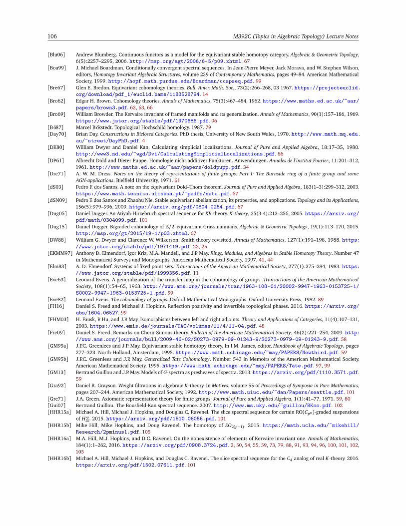
106 M392C (Topics in Algebraic Topology) Lecture Notes
[Blu06] Andrew Blumberg. Continuous functors as a model for the equivariant stable homotopy category. Algebraic & Geometric Topology,6(5):2257–2295, 2006. http://msp.org/agt/2006/6-5/p09.xhtml. 67
[Boa99] J. Michael Boardman. Conditionally convergent spectral sequences. In Jean-Pierre Meyer, Jack Morava, and W. Stephen Wilson,editors, Homotopy Invariant Algebraic Structures, volume 239 of Contemporary Mathematics, pages 49–84. American MathematicalSociety, 1999. http://hopf.math.purdue.edu/Boardman/ccspseq.pdf. 99
[Bre67] Glen E. Bredon. Equivariant cohomology theories. Bull. Amer. Math. Soc., 73(2):266–268, 03 1967. https://projecteuclid.org/download/pdf_1/euclid.bams/1183528794. 14
[Bro62] Edgar H. Brown. Cohomology theories. Annals of Mathematics, 75(3):467–484, 1962. https://www.maths.ed.ac.uk/~aar/papers/brown3.pdf. 62, 63, 66
[Bro69] William Browder. The Kervaire invariant of framed manifolds and its generalization. Annals of Mathematics, 90(1):157–186, 1969.https://www.jstor.org/stable/pdf/1970686.pdf. 96
[Bö87] Marcel Bökstedt. Topological Hochschild homology. 1987. 79[Day70] Brian Day. Constructions in Biclosed Categories. PhD thesis, University of New South Wales, 1970. http://www.math.mq.edu.
au/~street/DayPhD.pdf. 4[DK80] William Dwyer and Daniel Kan. Calculating simplicial localizations. Journal of Pure and Applied Algebra, 18:17–35, 1980.
http://www3.nd.edu/~wgd/Dvi/CalculatingSimplicialLocalizations.pdf. 86[DP61] Albrecht Dold and Dieter Puppe. Homologie nicht-additiver Funktoren. Anwendungen. Annales de l’institut Fourier, 11:201–312,
1961. http://www.maths.ed.ac.uk/~aar/papers/doldpupp.pdf. 34[Dre71] A. W. M. Dress. Notes on the theory of representations of finite groups. Part I: The Burnside ring of a finite group and some
AGN-applications. Bielfield University, 1971. 61[dS03] Pedro F. dos Santos. A note on the equivariant Dold–Thom theorem. Journal of Pure and Applied Algebra, 183(1–3):299–312, 2003.
https://www.math.tecnico.ulisboa.pt/~pedfs/note.pdf. 67[dSN09] Pedro F. dos Santos and Zhaohu Nie. Stable equivariant abelianization, its properties, and applications. Topology and its Applications,
156(5):979–996, 2009. https://arxiv.org/pdf/0804.0264.pdf. 67[Dug05] Daniel Dugger. An Atiyah-Hirzebruch spectral sequence for KR-theory. K-theory, 35(3-4):213–256, 2005. https://arxiv.org/
pdf/math/0304099.pdf. 101[Dug15] Daniel Dugger. Bigraded cohomology of Z/2–equivariant Grassmannians. Algebraic & Geometric Topology, 19(1):113–170, 2015.
http://msp.org/gt/2015/19-1/p03.xhtml. 67[DW88] William G. Dwyer and Clarence W. Wilkerson. Smith theory revisited. Annals of Mathematics, 127(1):191–198, 1988. https:
//www.jstor.org/stable/pdf/1971419.pdf. 22, 25[EKMM97] Anthony D. Elmendorf, Igor Kriz, M.A. Mandell, and J.P. May. Rings, Modules, and Algebras in Stable Homotopy Theory. Number 47
in Mathematical Surveys and Monographs. American Mathematical Society, 1997. 41, 44[Elm83] A. D. Elmendorf. Systems of fixed point sets. Transactions of the American Mathematical Society, 277(1):275–284, 1983. https:
//www.jstor.org/stable/pdf/1999356.pdf. 11[Eve63] Leonard Evens. A generalization of the transfer map in the cohomology of groups. Transactions of the American Mathematical
Society, 108(1):54–65, 1963. http://www.ams.org/journals/tran/1963-108-01/S0002-9947-1963-0153725-1/S0002-9947-1963-0153725-1.pdf. 59
[Eve82] Leonard Evens. The cohomology of groups. Oxford Mathematical Monographs. Oxford University Press, 1982. 89[FH16] Daniel S. Freed and Michael J. Hopkins. Reflection positivity and invertible topological phases. 2016. https://arxiv.org/
abs/1604.06527. 99[FHM03] H. Fausk, P. Hu, and J.P. May. Isomorphisms between left and right adjoints. Theory and Applications of Categories, 11(4):107–131,
2003. https://www.emis.de/journals/TAC/volumes/11/4/11-04.pdf. 48[Fre09] Daniel S. Freed. Remarks on Chern-Simons theory. Bulletin of the American Mathematical Society, 46(2):221–254, 2009. http:
//www.ams.org/journals/bull/2009-46-02/S0273-0979-09-01243-9/S0273-0979-09-01243-9.pdf. 58[GM95a] J.P.C. Greenlees and J.P. May. Equivariant stable homotopy theory. In I.M. James, editor, Handbook of Algebraic Topology, pages
277–323. North-Holland, Amsterdam, 1995. https://www.math.uchicago.edu/~may/PAPERS/Newthird.pdf. 59[GM95b] J.P.C. Greenlees and J.P. May. Generalized Tate Cohomology. Number 543 in Memoirs of the American Mathematical Society.
American Mathematical Society, 1995. https://www.math.uchicago.edu/~may/PAPERS/Tate.pdf. 97, 99[GM13] Bertrand Guillou and J.P. May. Models of G-spectra as presheaves of spectra. 2013. https://arxiv.org/pdf/1110.3571.pdf.
59[Gra92] Daniel R. Grayson. Weight filtrations in algebraic K-theory. In Motives, volume 55 of Proceedings of Symposia in Pure Mathematics,
pages 207–244. American Mathematical Society, 1992. http://www.math.uiuc.edu/~dan/Papers/seattle.pdf. 101[Gre71] J.A. Green. Axiomatic representation theory for finite groups. Journal of Pure and Applied Algebra, 1(1):41–77, 1971. 59, 80[Gui07] Bertrand Guillou. The Bousfield-Kan spectral sequence. 2007. http://www.ms.uky.edu/~guillou/BKss.pdf. 102[HHR15a] Michael A. Hill, Michael J. Hopkins, and Douglas C. Ravenel. The slice spectral sequence for certain RO(Cpn )-graded suspensions
of HZ. 2015. https://arxiv.org/pdf/1510.06056.pdf. 101[HHR15b] Mike Hill, Mike Hopkins, and Doug Ravenel. The homotopy of EO2(p−1). 2015. https://math.ucla.edu/~mikehill/
Research/2pminus1.pdf. 105[HHR16a] M.A. Hill, M.J. Hopkins, and D.C. Ravenel. On the nonexistence of elements of Kervaire invariant one. Annals of Mathematics,
184(1):1–262, 2016. https://arxiv.org/pdf/0908.3724.pdf. 2, 50, 54, 55, 59, 73, 79, 88, 91, 93, 94, 96, 100, 101, 102,105
[HHR16b] Michael A. Hill, Michael J. Hopkins, and Douglas C. Ravenel. The slice spectral sequence for the C4 analog of real K-theory. 2016.https://arxiv.org/pdf/1502.07611.pdf. 101
References 107
[Hil12] Michael A. Hill. The equivariant slice filtration: a primer. Homology, Homotopy and Applications, 14(2):143–166, 2012. https://intlpress.com/site/pub/files/_fulltext/journals/hha/2012/0014/0002/HHA-2012-0014-0002-a009.pdf. 101
[Hil15] Michael A. Hill. On the fate of η3 in higher analogues of real bordism. 2015. https://arxiv.org/pdf/1507.08083.pdf.101
[Hir03] Philip S. Hirschhorn. Model Categories and Their Localizations. Number 99 in Mathematical Surveys and Monographs. AmericanMathematical Society, 2003. 42
[HKO11] P. Hu, I. Kriz, and K. Ormsby. The homotopy limit problem for Hermitian K-theory, equivariant motivic homotopy theory and motivicreal cobordism. Advances in Mathematics, 228(1):434–480, 2011. http://www.math.lsa.umich.edu/~ikriz/ar1012.pdf.101
[HL16] Michael Hopkins and Jacob Lurie. Ambidexterity in K(n)-local stable homotopy theory. 2016. http://www.math.harvard.edu/~lurie/papers/Ambidexterity.pdf. 100
[HM92] Lars Hesselholt and Ib Madsen. The S1-Tate spectrum for J . In Samuel Gitler, editor, Papers in honor of Jose Adem, volume 37,pages 215–240, 1992. 99
[HM03] Lars Hesselholt and Ib Madsen. On the K-theory of local fields. Annals of Mathematics, 158(1):1–113, 2003. http://annals.math.princeton.edu/wp-content/uploads/annals-v158-n1-p01.pdf. 97
[HM16] Michael A. Hill and Lennart Meier. The C2-spectrum Tmf1(3) and its invertible modules. 2016. https://arxiv.org/pdf/1507.08115. 101
[Hov99] Mark Hovey. Model Categories. Mathematical Surveys and Monographs. American Mathematical Society, 1999. 2[Hoy14] Rolf Hoyer. Two topics in stable homotopy theory. PhD thesis, The University of Chicago, 2014. 87[HS14] Drew Heard and Vesna Stojanoska. K-theory, reality, and duality. Journal of K-theory, 14(3):526–555, 2014. https://arxiv.
org/abs/1401.2581. 104, 105[HSS00] Mark Hovey, Brooke Shipley, and Jeff Smith. Symmetric spectra. J. Amer. Math. Soc, 13:149–208, 2000. http://www.math.
uiuc.edu/K-theory/0265/symm.pdf. 38[HY17] Michael A. Hill and Carolyn Yarnall. A new formulation of the equivariant slice filtration with applications to Cp-slices. 2017.
https://arxiv.org/pdf/1703.10526.pdf. 101[Ill72] Sören Illman. Equivariant Algebraic Topology. PhD thesis, Princeton University, 1972. http://archive.numdam.org/ARCHIVE/
AIF/AIF_1973__23_2/AIF_1973__23_2_87_0/AIF_1973__23_2_87_0.pdf. 6[Imp95] R. Impagliazzo. A personal view of average-case complexity. In Proceedings of Structure in Complexity Theory. Tenth Annual IEEE
Conference, pages 134–147. IEEE, 1995. 31[Kel84] G.M. Kelley. Basic Concepts in Enriched Category Theory. Number 64 in Lecture Notes in Mathematics. Cambridge University Press,
1984. http://www.tac.mta.ca/tac/reprints/articles/10/tr10.pdf. 4[Ker60] Michael Kervaire. A manifold which does not admit any differentiable structure. Commentarii Mathematicii Helvetici, 34:257–270,
1960. http://www.maths.ed.ac.uk/~aar/papers/kervarf.pdf. 96[Kuh04a] Nicholas J. Kuhn. Tate cohomology and periodic localization of polynomial functors. Inventiones mathematicae, 157(2):345–370,
2004. https://arxiv.org/pdf/math/0307173.pdf. 55[Kuh04b] Nick Kuhn. The McCord model for the tensor product of a space and a commutative ring spectrum. In Gregory Arone, John
Hubbuck, Ran Levi, and Michael Weiss, editors, Categorical Decomposition Techniques in Algebraic Topology, volume 215 of Progressin Mathematics, pages 213–235. Birkhäuser Basel, 2004. https://arxiv.org/pdf/math/0202042.pdf. 66, 67
[Lan67] Peter S. Landweber. Fixed point free conjugations on complex manifolds. Annals of Mathematics, 86(3):491–502, 1967. https://www.jstor.org/stable/pdf/1970612.pdf. 96
[Lew78] L. Gaunce Lewis. The Stable Category and Generalized Thom Spectra. PhD thesis, The University of Chicago, 1978. 62[Lew80] L. Gaunce Lewis. The theory of Green functors. 1980. http://web.math.rochester.edu/people/faculty/doug/
otherpapers/Lewis-Green.pdf. 80[Lew88] L. Gaunce Lewis. The RO(G)-graded equivariant ordinary cohomology of complex projective spaces with linear Z/p actions. In
Tammo tom Dieck, editor, Algebraic Topology and Transformation Groups, volume 1361 of Lecture Notes in Mathematics, pages53–122. Springer Berlin Heidelberg, 1988. 67, 70, 71, 72
[Lew91] L. Gaunce Lewis. Is there a convenient category of spectra? Journal of Pure and Applied Algebra, 73(3):233–246, 1991. 43[LM06] L. Gaunce Lewis and Michael A. Mandell. Equivariant universal coefficient and Künneth spectral sequences. Proceedings of the
London Mathematical Society, 92(2):505–544, 2006. https://arxiv.org/abs/math/0410162. 62[LMS86] L. Gaunce Lewis Jr., J. Peter May, and Mark Steinberger. Equivariant Stable Homotopy Theory. Number 1213 in Lecture Notes
in Mathematics. Springer Berlin Heidelberg, 1986. https://www.math.uchicago.edu/~may/BOOKS/equi.pdf. 2, 30, 34,37, 41, 48, 50, 59
[Lur09] Jacob Lurie. On the classification of topological field theories. Current Developments in Mathematics, 2008:129–280, 2009.http://www-math.mit.edu/~lurie/papers/cobordism.pdf. 27
[Mac78] Saunders Mac Lane. Categories for the Working Mathematician. Number 5 in Graduate Texts in Mathematics. Springer-Verlag NewYork, 1978. 2
[Mah77] Mark Mahowald. A new infinite family in 2πs∗. Topology, 16(3):249–256, 1977. 96
[Man01] Michael A. Mandell. E∞-algebras and p-adic homotopy theory. Topology, 40(1):43–94, 2001. http://hopf.math.purdue.edu/Mandell/einf.pdf. 29
[Man12] Michael A. Mandell. The smash product for derived categories in stable homotopy theory. Advances in Mathematics, 230(4–6):1531–1556, 2012. https://arxiv.org/pdf/1004.0006.pdf. 54
[Mau63] C.R.F. Maunder. The spectral sequence of an extraordinary cohomology theory. Mathematical Proceedings of the Cambridge Philosoph-ical Society, 59(3):567–574, 1963. https://www.cambridge.org/core/services/aop-cambridge-core/content/view/S0305004100037245. 101
108 M392C (Topics in Algebraic Topology) Lecture Notes
[May72] Peter May. The Geometry of Iterated Loop Spaces. Number 271 in Lecture Notes in Mathematics. Springer-Verlag, 1972. https://www.math.uchicago.edu/~may/BOOKS/geom_iter.pdf. 13, 76
[May77] Peter May. E∞-ring spaces and E∞-ring spectra. Lecture Notes in Mathematics. Springer-Verlag Berlin Heidelberg, 1977. https://www.math.uchicago.edu/~may/BOOKS/e_infty.pdf. 96
[May87] J. P. May. A generalization of Smith theory. Proceedings of the American Mathematical Society, 101(4):728–730, 1987. https://math.uchicago.edu/~may/PAPERS/57.pdf. 22
[May96] Peter May, editor. Equivariant Homotopy and Cohomology Theory, volume 91 of CBMS Regional Conference Series in Mathematics.American Mathematical Society, 1996. https://www.math.uchicago.edu/~may/BOOKS/alaska.pdf. 2, 22, 37
[May99] Peter May. A Concise Course in Algebraic Topology. Chicago Lectures in Mathematics. The University of Chicago Press, 1999.https://www.math.uchicago.edu/~may/CONCISE/ConciseRevised.pdf. 2, 10
[May03] J.P. May. The Wirthmüller isomorphism revisited. Theory and Applications of Categories, 11(5):132–142, 2003. https://www.emis.de/journals/TAC/volumes/11/5/11-05.pdf. 48
[May09a] J.P. May. The construction of E∞ ring spaces from bipermutative categories. Geometry & Topology Monographs, 16:283–330, 2009.https://www.math.uchicago.edu/~may/PAPERS/Final2.pdf. 96
[May09b] J.P. May. What are E∞ ring spaces good for? Geometry & Topology Monographs, 16:331–365, 2009. https://www.math.uchicago.edu/~may/PAPERS/Final3.pdf. 96
[May09c] J.P. May. What precisely are E∞ ring spaces and E∞ ring spectra? Geometry & Topology Monographs, 16:215–282, 2009.https://www.math.uchicago.edu/~may/PAPERS/Final1.pdf. 96
[Maz13] Kristen Mazur. On the Structure of Mackey Functors and Tambara Functors. PhD thesis, University of Virginia, 2013. https://sites.lafayette.edu/mazurk/files/2013/07/Mazur-Thesis-4292013.pdf. 87
[McC69] M.C. McCord. Classifying spaces and infinite symmetric products. Transactions of the American Mathematical So-ciety, 146:273–298, 1969. http://www.ams.org/journals/tran/1969-146-00/S0002-9947-1969-0251719-4/S0002-9947-1969-0251719-4.pdf. 66
[Mil71] James Milgram. Problems presented to the 1970 AMS symposium on algebraic topology. In A. Liulevicius, editor, Algebraic Topology,volume 22 of Proceedings of Symposia in Pure Mathematics, pages 187–201. American Mathematical Society, 1971. 96
[Mit94] Stephen A. Mitchell. On the Lichtenbaum-Quillen conjectures from a stable homotopy-theoretic viewpoint. In Gunnar E. Carlsson,Ralph L. Cohen, Wu-Chung Hsiang, and John D. S. Jones, editors, Algebraic Topology and Its Applications, pages 163–240. SpringerNew York, New York, NY, 1994. 101
[MM02] M.A. Mandell and J.P. May. Equivariant orthogonal spectra and S-modules. Number 755 in Memoirs of the American MathematicalSociety. American Mathematical Society, 2002. https://www.math.uchicago.edu/~may/PAPERS/MMMFinal.pdf. 39
[MMSS01] M. A. Mandell, J. P. May, S. Schwede, and B. Shipley. Model categories of diagram spectra. Proceedings of the London MathematicalSociety, 82(2):441–512, 2001. https://www.math.uchicago.edu/~may/PAPERS/mmssLMSDec30.pdf. 32, 37, 39
[MNN17] Akhil Mathew, Niko Naumann, and Justin Noel. Nilpotence and descent in equivariant stable homotopy theory. Advances inMathematics, 305:994–1084, 2017. https://arxiv.org/pdf/1507.06869.pdf. 99
[Mos57] G. D. Mostow. Equivariant embeddings in Euclidean space. Annals of Mathematics, 65(3):432–446, 1957. https://www.jstor.org/stable/pdf/1970055.pdf. 35
[Nak12a] Hiroyuki Nakaoka. Ideals of Tambara functors. Advances in Mathematics, 230(4–6):2295–2331, 2012. https://arxiv.org/pdf/1101.5982.pdf. 87
[Nak12b] Hiroyuki Nakaoka. On the fractions of semi-Mackey and Tambara functors. Journal of Algebra, 352(1):79–103, 2012. https://arxiv.org/pdf/1103.3991.pdf. 87
[Nak14] Hiroyuki Nakaoka. The spectrum of the Burnside Tambara functor on a finite cyclic p-group. Journal of Algebra, 398:21–54, 2014.https://arxiv.org/pdf/1301.1453.pdf. 87
[Nee96] Amnon Neeman. The Grothendieck duality theorem via Bousfield’s techniques and Brown representability. Journal of the AmericanMathematical Society, 9(1):205–236, 1996. https://www.jstor.org/stable/2152846. 62, 63
[Pal57] Richard S. Palais. Imbedding of compact, differentiable transformation groups in orthogonal representations.Journal of Mathematics and Mechanics, 6(5):673–678, 1957. http://vmm.math.uci.edu/PalaisPapers/ImbeddingCmpctDiffTransfGrpsInOrthogReps.pdf. 35
[Rie14] Emily Riehl. Categorical Homotopy Theory. Cambridge University Press, 2014. http://www.math.harvard.edu/~eriehl/cathtpy.pdf. 2, 4, 13
[Rie16] Emily Riehl. Category Theory in Context. Aurora: Dover Modern Math Originals. Dover Publications, 2016. http://www.math.jhu.edu/~eriehl/context.pdf. 2, 6
[Rub17] Jonathan Rubin. On the realization problem for N∞ operads. 2017. https://arxiv.org/pdf/1705.03585.pdf. 78[RW80] Douglas C. Ravenel and W. Stephen Wilson. The Morava K-theories of Eilenberg-MacLane spaces and the Conner-Floyd conjecture.
American Journal of Mathematics, 102(4):691–748, 1980. https://web.math.rochester.edu/people/faculty/doug/mypapers/emspace.pdf. 100
[Sch12] S. Schwede. Symmetric spectra. 2012. http://www.math.uni-bonn.de/~schwede/SymSpec-v3.pdf. 38, 40[Sch16] S. Schwede. Lectures on equivariant stable homotopy theory. 2016. http://www.math.uni-bonn.de/~schwede/
equivariant.pdf. 96[Sch17] S. Schwede. Global homotopy theory. 2017. http://www.math.uni-bonn.de/~schwede/global.pdf. 40[Seg78] G. Segal. Some results in equivariant homotopy theory. 1978. 67, 91[Shi89] Kazuhisa Shimakawa. Infinite loop G-spaces associated to monoidal G-graded categories. Publ. Res. Inst. Math. Sci., 25(2):239–262,
1989. https://www.ems-ph.org/journals/show_abstract.php?issn=0034-5318&vol=25&iss=2&rank=3. 67, 91[Shi91] Kazuhisa Shimakawa. A note on ΓG -spaces. Osaka J. Math., 28(2):223–228, 1991. https://projecteuclid.org/download/
pdf_1/euclid.ojm/1200783054. 91

References 109
[SS00] Stefan Schwede and Brooke E. Shipley. Algebras and modules in monoidal model categories. Proceedings of the London MathematicalSociety, 80(2):491–511, 2000. http://www.math.uni-bonn.de/people/schwede/AlgebrasModules.pdf. 44
[Ste16] Marc Stephan. On equivariant homotopy theory for model categories. Homology, Homotopy and Applications, 18(2):183–208,2016. https://arxiv.org/pdf/1308.0856.pdf. 11
[Str12] Neil Strickland. Tambara functors. 2012. https://arxiv.org/pdf/1205.2516.pdf. 80[Sul74] Denis Sullivan. Genetics of homotopy theory and the Adams conjecture. Annals of Mathematics, 100(1):1–79, 7 1974. http:
//math1.unice.fr/~cazanave/Gdt/ImJ/Sullivan.pdf. 28[Sul77] D. Sullivan. Infinitesimal Computations in Topology. Number 47 in Publications mathématiques de l’I.H.É.S. 1977.
http://archive.numdam.org/ARCHIVE/PMIHES/PMIHES_1977__47_/PMIHES_1977__47__269_0/PMIHES_1977__47__269_0.pdf. 27, 29
[Sul05] Denis Sullivan. Geometric Topology: Localization, Periodicity, and Galois Symmetry. Number 8 in K-Monographs in Mathematics.Springer Verlag, 2005. http://www.maths.ed.ac.uk/~aar/books/gtop.pdf. 25, 28, 31
[Tam93] Daisuke Tambara. On multiplicative transfer. Comm. Algebra, 21(4):1393–1420, 1993. 59, 86[Tho54] René Thom. Quelques propriétés globales des variétés differentiables. PhD thesis, University of Paris, 1954. http://www.maths.
ed.ac.uk/~aar/papers/thomcob.pdf. 34[Ull12] John Ullman. Tambara functors and commutative ring spectra. 2012. https://arxiv.org/pdf/1304.4912.pdf. 95[Web00] Peter Webb. A guide to Mackey functors. In M. Hazewinkel, editor, Handbook of Algebra, volume 2 of Handbook of Algebra, pages
805–836. North-Holland, 2000. http://www-users.math.umn.edu/~webb/Publications/GuideToMF.pdf. 61[Yar15] Carolyn Yarnall. The slices of Sn ∧HZ for cyclic p-groups. 2015. https://arxiv.org/pdf/1510.02077. 101