arxiv:gr-qc/9509036v4 12 apr 1996
TRANSCRIPT
arX
iv:g
r-qc
/950
9036
v4 1
2 A
pr 1
996
preprint - UTF 361gr-qc/9509036
A Bisognano-Wichmann-like Theorem in a Certain
Case of a Non Bifurcate Event Horizon related to an
Extreme Reissner-Nordstrom Black Hole
Valter Moretti 1
Dipartimento di Fisica, Universita di Trento and Istituto Nazionale di Fisica Nucleare,Gruppo Collegato di Trento,Via Sommarive 14 I-38050 Povo (TN) Italy
Stefan Steidl 2
Institut fur Theoretische Physik der Universitat Innsbruck, Victor-Franz-Hess-Haus,Technikerstraße 25/2 A-6020 Innsbruck Austria
July-August-September 1995
Abstract:Thermal Wightman functions of a massless scalar field are studied within the frame-work of a “near horizon” static background model of an extremal R-N black hole.This model is built up by using global Carter-like coordinates over an infinite set ofBertotti-Robinson submanifolds glued together. The analytical extendibility beyondthe horizon is imposed as constraints on (thermal) Wightman’s functions defined ona Bertotti-Robinson sub manifold. It turns out that only the Bertotti-Robinson vac-uum state, i.e. T = 0, satisfies the above requirement. Furthermore the extensionof this state onto the whole manifold is proved to coincide exactly with the vacuumstate in the global Carter-like coordinates. Hence a theorem similar to Bisognano-Wichmann theorem for the Minkowski space-time in terms of Wightman functionsholds with vanishing “Unruh-Rindler temperature”. Furtermore, the Carter-like vac-uum restricted to a Bertotti-Robinson region, resulting a pure state there, has van-ishing entropy despite of the presence of event horizons. Some comments on the realextremal R-N black hole are given.
PACS number(s): 04.62.+v, 04.70.Dy, 11.10.Wx
1e-mail: [email protected]: [email protected]
1
Introduction
In a space-time with non empty intersection event horizons, i.e. Rindler-Schwarzschild-like space-time, several methods for determining the possible equilibrium state of a scalarfield propagating therein exist. They select one special temperature only, the Rindler-Unruh-Hawking temperature. These theorems use the KMS condition [1] and the HaagNarnhofer Stein principle (i.e., the ”Haag scaling prescription”) [2, 3] or demand a sta-tionary and Hadamard behaviour of the Wightman functions [4].These theorems can not be employed in the case of an extremal Reissner-Nordstrom blackhole due to the appearence of a null surface gravity as well as a non-bifurcate event hori-zons. In fact the future event horizon and the past event horizon do not intersect there.However, Anderson, Hiscock and Loranz [5] proved that only the Reissner-Nordstrom vac-uum state has a regular stress-tensor on the horizon and thus only this state is a possibleequilibrium state in the framework of semiclassical quantum gravity. Finally, in recentworks [10, 6], Moretti shows that the Haag Narnhofer and Stein principle for the behaviourof Wightman’s function on the horizon of a black hole results to be unable to determinethe really admissible thermal quantum states in the case of an extremal R-N black hole,but a further development of the previous principle, the Hessling principle 3[12, 10, 6]determines only the Reissner-Nordstrom quantum vacuum as physically admissible (i.e.T = 0). Similar result, but using very different analysis, appeared in [7]. These facts seemto improve the topological result obtained by the method of the elimination of conicalsingularities from the Euclidean, time extended manifold, which accepts any value of thetemperature for a R-N black hole[9, 11].Almost all the previously mentioned papers deal with quantum field states at least definedin a certain space-time region (boundary included) bounded by event horizons, e.g. theexternal region of a black hole.On the other hand, it is obvious that the classical field is not blocked by the horizons andthus it seems to be necessary to demand the existence of global extensions of physicallysensible quantum field states. This request result to be satisfyed by the Minkowski vac-uum in the Rindler wedge theory and by the Hartle-Hawking state in the Schwarzschildblack hole theory.As well-known, the extremal Reissner-Nordstrom manifold can be maximally extendedinto Carter’s manifold and thus it seems to be interesting to study quantum field statesdefined on the whole Carter manifold (if they exist).In this paper, we shall study a “near horizon” model of Carter’s and Reissner-Nordstrommanifolds. Following an algebraic approach to quantum field theory and starting fromKMS quantum states initially defined in a Reissner-Nordstrom-like submanifold only, weshall study the existence of analytical extensions beyond the horizons of their Wightmanfunctions and thus in the whole Carter-like manifold.In particular, as our first result, we shall prove the possibility of an algebraic quantumfield formulation on our manifold despite of the fact that this is non globally hyperbolic.Moreover, as our second result, we shall prove that only the approximated vacuum statecorresponding to the Reissner-Nordstrom vacuum state (with zero temperature) can be
3Roughly speaking, these two principles correspond respectively to a weaker and a stronger versionof a Quantum Einstein’s Equivalence Principle. They require a weaker and a stronger “Minkowskianbehaviour” of two point Wightman functions in the limit of vanishing geodesical distance between thearguments.
2
extended beyond the horizons.Furthermore we shall see that there exists a relation between our model-manifold endowedwith Bertotti-Robinson sub-manifolds and Minkowski space-time endowed with the well-known couple of Rindler wedges. These two structures act as “toy models” of two differentkinds of black holes: the extremal R-N black hole and the eternal Schwarzschild blackhole respectively. Implementing this analogy, as our third result, we shall recover theequivalent of the the Bisognano-Wichmann theorem for the Minkowski space-time[27]. Inthis contest, the analog of the Minkowski vacuum is the vacuum defined with respectto the global Carter-like coordinates of our manifold. The β = 2π-Rindler-KMS statecorresponds to the vacuum of the R-N-like coordinates.Thus, an important difference arises. The analog of the Rindler-Unruh temperature isnow zero and thus no KMS prescription appears, but the stationarity of the state remains,i.e., the functional dependency of only the difference of the temporal arguments.In Section 1 we shall introduce the well-known Carter representation for a maximallyanalytically extendible manifold for an extremal R-N black hole. Furthermore, we shallperform the necessary approximations in order to deal with a neighbourhood of the hori-zon.In Section 2, using approximated Carter coordinates and the Bertotti-Robinson metric,we shall construct a “near horizon” toy model of Carter’s manifold which results to be nonglobally hyperbolic. We shall prove that it is possible to define a quantum field theory.Finally, we shall study the analytical extension of Wightman’s functions beyond the hori-zons proving also a Bisognano-Wichmann-like theorem in terms of Wightman functions.In Section 3, we shall point out our conclusions and we shall look at the real extremalR-N black hole.
1 Carter’s Manifold and Approximations near its Hori-
zons
The general form of Reissner-Nordstrom black-hole metric is given by [22]
ds2 = −(
1− 2M
r+
Q2
r2
)2
dt2 +1
(
1− 2Mr
+ Q2
r2
)2dr2 + r2
(
dθ2 + sin2 θdϕ2)
,
where M is the mass and Q the charge of the black hole. We are interested in extremalcase Q = M . Thus we have
ds2 = −(
1− M
r
)2
dt2 +1
(
1− Mr
)2dr2 + r2
(
dθ2 + sin2 θdϕ2)
.
For sake of simplicity, we shall chose an extremal black hole of unit mass by a suit-able choice of the units of measure. In addition, we shall use the abbreviation dΩ2 :=(
dθ2 + sin2 θdϕ2)
. Thus, our metric reads
ds2 = −(
1− 1
r
)2
dt2 +1
(
1− 1r
)2dr2 + r2dΩ2 . (1)
3
As well-known, the above chart does not cover the whole manifold as ds2 is singularat r = 1. This inconvenience can be avoided, following the Schwarzschild case, by intro-ducing Kruskal-like coordinates4, i.e., Carter’s coordinates [14]. These define a maximallyanalytically extended manifold obtained from the R-N manifold (r > 1). To begin with,we introduce two functions u(t, r) and w(t, r) by
u = r∗ + t , (2)
w = r∗ − t , (3)
where r∗ is given by the invertible function of r > 1
r∗(r) =∫
dr(
1− 1r
)2 = rr − 2
r − 1+ 2 ln |r − 1| . (4)
Let us introduce Carter’s coordinates in the Reissner-Nordstrom manifold T,R, θ, ϕ[14]5 through the equations
u = − cot (T +R) , (5)
w = +cot (T − R) , (6)
and thus
2T = cot−1(w)− cot−1(u) , (7)
2R = − cot−1(w)− cot−1(u) , (8)
where T ∈]− π/2,+π/2[ and R ∈]0, π[. The metric in Eq.(1) reads now
ds2 = Q(
−dT 2 + dR2)
+ r2dΩ2 , (9)
where Q is given by
Q =(
1− 1
r
)2
csc2 (T +R) csc2 (T −R) . (10)
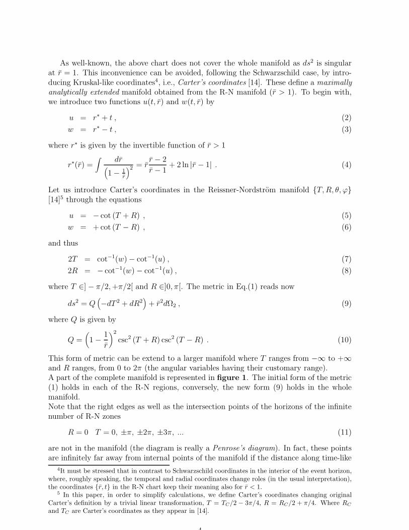
This form of metric can be extend to a larger manifold where T ranges from −∞ to +∞and R ranges, from 0 to 2π (the angular variables having their customary range).A part of the complete manifold is represented in figure 1. The initial form of the metric(1) holds in each of the R-N regions, conversely, the new form (9) holds in the wholemanifold.Note that the right edges as well as the intersection points of the horizons of the infinitenumber of R-N zones
R = 0 T = 0, ±π, ±2π, ±3π, ... (11)
are not in the manifold (the diagram is really a Penrose’s diagram). In fact, these pointsare infinitely far away from internal points of the manifold if the distance along time-like
4It must be stressed that in contrast to Schwarzschild coordinates in the interior of the event horizon,where, roughly speaking, the temporal and radial coordinates change roles (in the usual interpretation),the coordinates r, t in the R-N chart keep their meaning also for r < 1.
5 In this paper, in order to simplify calculations, we define Carter’s coordinates changing originalCarter’s definition by a trivial linear transformation, T = TC/2 − 3π/4, R = RC/2 + π/4. Where RC
and TC are Carter’s coordinates as they appear in [14].
4
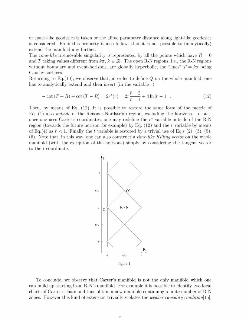
or space-like geodesics is taken or the affine parameter distance along light-like geodesicsis considered. From this property it also follows that it is not possible to (analytically)extend the manifold any further.The time-like irremovable singularity is represented by all the points which have R = 0and T taking values different from kπ, k ∈ ZZ. The open R-N regions, i.e., the R-N regionswithout boundary and event-horizons, are globally hyperbolic, the “lines” T = kπ beingCauchy-surfaces.Returning to Eq.(10), we observe that, in order to define Q on the whole manifold, onehas to analytically extend and then invert (in the variable r)
− cot (T +R) + cot (T −R) = 2r∗(r) = 2rr − 2
r − 1+ 4 ln |r − 1| , (12)
Then, by means of Eq. (12), it is possible to restore the same form of the metric ofEq. (1) also outside of the Reissner-Nordstrom region, excluding the horizons. In fact,once one uses Carter’s coordinates, one may redefine the r∗ variable outside of the R-Nregion (towards the future horizon for example) by Eq. (12) and the r variable by meansof Eq.(4) as r < 1. Finally the t variable is restored by a trivial use of Eq.s (2), (3), (5),(6). Note that, in this way, one can also construct a time-like Killing vector on the wholemanifold (with the exception of the horizons) simply by considering the tangent vectorto the t coordinate.
T
O’
R - N
R
O
π
0
−π
0 π / 2 π
− π / 2
π / 2
figure 1
To conclude, we observe that Carter’s manifold is not the only manifold which onecan build up starting from R-N’s manifold. For example it is possible to identify two localcharts of Carter’s chain and thus obtain a new manifold containing a finite number of R-Nzones. However this kind of extension trivially violates the weaker causality condition[15],
5

hence it is not clear whether a quantum field theory can be defined there6.
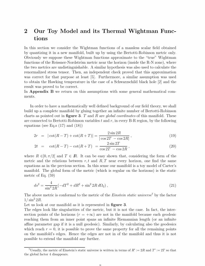
Now we shall consider an approximated metric near the horizons. In the shaded regionnear the horizons represented in figure 2, the metric (9) can be approximated by a staticmetric
ds2 ∼ ds20 :=4
sin2 2R(−dT 2 + dR2) + dΩ2 . (13)
The vector ∂T defines an approximated time-like Killing vector near the horizons.In the same region, but considering R-N coordinates, ds2 can be approximated by theBertotti-Robinson metric [21], as well-known [8]. Thus we have
ds2 ∼ ds2BR :=−dt2 + dr2 + dΩ2
r2, (14)
where
r := −r∗ if R > T or (15)
r := +r∗ if R < T . (16)
O
Tπ
0 π
figure 2
R
1 > r = const.
1 < r = const.
t = const.
π / 2
− π / 2
π / 2 W
UO’
Finally, in the considered region, the transformation law between r, t and R, T is
2r ∼ | cot(R− T ) + cot(R + T )| = 2 sin 2R
| cos 2T − cos 2R| , (17)
2t ∼ cot(R− T )− cot(R + T ) =2 sin 2T
cos 2T − cos 2R, (18)
All the previous approximations are carefully examined in Appendix A (see also [8]).
6However, Kay et al. investigated the possibilities of a QFT in similar backgrounds [16, 20] recently.
6
2 Our Toy Model and its Thermal Wightman Func-
tions
In this section we consider the Wightman functions of a massless scalar field obtainedby quantizing it in a new manifold, built up by using the Bertotti-Robinson metric only.Obviously we suppose these Wightman functions approximate to the “true” Wightmanfunctions of the Reissner-Nordstrom metric near the horizon (inside the R-N zone), wherethe two metrics are undistinguishable. A similar hypothesis was also used to calculate therenormalized stress tensor. Then, an independent check proved that this approximationwas correct for that purpose at least [5]. Furthermore, a similar assumption was usedto obtain the Hawking temperature in the case of a Schwarzschild black hole [2] and theresult was proved to be correct.In Appendix B we return on this assumptions with some general mathematical com-ments.
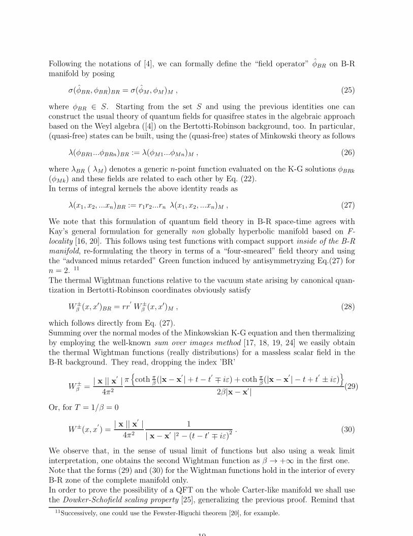
In order to have a mathematically well defined background of our field theory, we shallbuild up a complete manifold by gluing together an infinite number of Bertotti-Robinsoncharts as pointed out in figure 3. T and R are global coordinates of this manifold. Theseare connected to Bertotti-Robinson variables t and r, in every B-R region, by the followingequations (see Eq.s (17) and (18))
2r = | cot(R− T ) + cot(R + T )| = 2 sin 2R
| cos 2T − cos 2R| , (19)
2t = cot(R− T )− cot(R + T ) =2 sin 2T
cos 2T − cos 2R, (20)
where R ∈]0, π/2[ and T ∈ IR. It can be easy shown that, considering the form of themetric and the relations between r, t and R, T near every horizon, one find the sameequations as in the previous section. In this sense our manifold is a toy model of Carter’smanifold. The global form of the metric (which is regular on the horizons) is the staticmetric of Eq. (59)
ds2 =4
sin2 2R(−dT 2 + dR2 + sin2 2R dΩ2) , (21)
The above metric is conformal to the metric of the Einstein static universe7 by the factor1/ sin2 2R.Let us look at our manifold as it is represented in figure 3.The edges look like singularities of the metric, but it is not the case. In fact, the inter-section points of the horizons (r = +∞) are not in the manifold because each geodesicreaching them from an inner point spans an infinite Riemannian length (or an infiniteaffine parameter gap if it is a null geodesic). Similarly, by calculating also the geodesicswhich reach r = 0, it is possible to prove the same property for all the remaining pointson the manifold’s edges. Hence the edges are not in of the manifold and thus it is notpossible to extend the manifold any further.
7Usually, the metric of Einstein’s static universe is written in terms of R′ := 2R and T ′ := 2T so thatthe global factor 4 disappears.
7

r =
r =
r =
R
r = 0
r = 0
figure 3
r = 0
U
W
B - R
B - R
B - R
r = 0
r = 0
T
Finally we stress that passing to the Euclidean time tE = it and using r, tE coordi-nates, no conical singularity arises for any choice of the Euclidean time period β8. Hence,following [9] and [11], we should accept all the values of the temperature of the KMSstates defined inside of a B-R zone.
It is possible to compare Carter’s manifold to Kruskal manifold in the following sense.Let us consider Kruskal manifold. There, the metric looks like that of a Rindler space ifSchwarzschild’s coordinates are used, or, that of a Minkowski space if Kruskal’s coordi-nates are adopted. Also, the transformation laws between these two coordinate systemslocally resemble the corresponding transformation laws in the Minkowski manifold. Fur-thermore, near the horizon, the Kruskal time defines an approximated time-like Killingvector which becomes a global time-like Killing vector in the Minkowski space-time.Considering Carter’s manifold, the same features will arise. We have to consider Carter’scoordinates as Kruskal’s coordinates, our global Carter-like model as a Minkowski’s mani-fold and Bertotti-Robinson manifold as a Rindler wedge. Then, near the horizons, Carter’smetric looks like that of Bertotti-Robinson if we use Reissner-Nordstrom coordinates, orthe metric conformal to the Einstein static metric if we used Carter’s coordinates and soon. In particular, the approximated time-like Killing vector near the horizon in Carter’smanifold becomes an exact time-like Killing vector in our Carter-like global manifold.Roughly speaking, the quantum field theory in a Rindler wedge on the background of a
8The point r = 0 which (which is a conical singularity of the Euclidean manifold in the Rindler orSchwarzschild cases) does not belong to the manifold now.
8

Minkowski space-time appears as a simplified quantum field theory in a Schwarzschildspace-time on the background of a Kruskal manifold. The coincidence of the Unruh-Rindler state with the Minkowski vacuum (Bisognano-Wichmann theorem) appears asa simplified version of the coincidence of β = 4π-Schwarzschild-KMS state 9 with theHartle-Hawking state. It is reasonable to expect a similar situation for a quantum fieldtheory on the Carter manifold.In the following we want to implement a part of this idea proving, as our third result, theequivalent of the Bisognano-Wichmann theorem in our Carter-like manifold.Like Carter’s manifold, our Carter-like manifold is not globally hyperbolic [15, 22] be-cause near the edge r = 0 it is possible to find a pair of points p, q with J+(p) ∩ J−(q)not closed and thus not compact; furthermore, differently from Carter’s manifold, all the“patch manifolds” (B-R zones) are non globally hyperbolic. We shall prove, that insideany of these regions as well as in the whole Carter-like manifold, a “quasi-standard”quasifree scalar field theory can be defined.
2.1 Possibility of a QFT
In order to point out the possibility of a QFT on our manifolds, we shall follow thealgebraic approach used in [4] based on Weyl algebra.First we consider the B-R submanifolds. From now on, we shall understand x0, x1, x2, x3
(posing also t := x0, x ≡ (x1, x2, x3) and r :=| x |) as Minkowski coordinates in Minkowskispace as well as Bertotti-Robinson coordinates in the Bertotti-Robinson space.Let us start by considering that a very simple connection between the solutions of themassless Klein-Gordon equation in Minkowski space and in the Bertotti-Robinson spaceexists. If φ(x, t)M indicates a generic C∞ solution with compact spatial support of themassless Minkowskian K-G equation, then
φ(x, t)BR = rφ(x, t)M , (22)
where r > 0, t ∈ IR and φ(x, t)BR is a solution of the massless Bertotti-Robinson K-Gequation of the same order of smoothness but without compact spatial support in general.In order to build up the Weyl algebra [26, 23, 4], we have to consider the following bilinearsymplectic form or indefinite scalar product
σ(φ1, φ2) :=∫
t=const.φ1
↔
∇µφ2 nµ√h dx1dx2dx3 , (23)
where n is the normal (and normalized) vector to the Cauchy surface t =constant and his the determinant of the induced metric on this surface.In the case of Minkowski space the above surfaces are Cauchy surfaces, but this is nottrue in the case of Bertotti-Robinson space and thus we can not deal with the standardtheory. However, if we decide to restrict the possible vector space S of solutions of theK-G equation by considering only the scalar fields on the left hand side of Eq. (22)10, weshall trivially find the following identity
σ(φBR1, φBR2)BR = σ(φM1, φM2)M . (24)
9Using opportune units of measure.10Roughly speaking, this is similar to a boundary condition requirement on the fields solutions of the
K-G equation in the B-R manifold.
9
Following the notations of [4], we can formally define the “field operator” φBR on B-Rmanifold by posing
σ(φBR, φBR)BR = σ(φM , φM)M , (25)
where φBR ∈ S. Starting from the set S and using the previous identities one canconstruct the usual theory of quantum fields for quasifree states in the algebraic approachbased on the Weyl algebra ([4]) on the Bertotti-Robinson background, too. In particular,(quasi-free) states can be built, using the (quasi-free) states of Minkowski theory as follows
λ(φBR1...φBRn)BR := λ(φM1...φMn)M , (26)
where λBR ( λM) denotes a generic n-point function evaluated on the K-G solutions φBRk
(φMk) and these fields are related to each other by Eq. (22).In terms of integral kernels the above identity reads as
λ(x1, x2, ...xn)BR := r1r2...rn λ(x1, x2, ...xn)M , (27)
We note that this formulation of quantum field theory in B-R space-time agrees withKay’s general formulation for generally non globally hyperbolic manifold based on F-locality [16, 20]. This follows using test functions with compact support inside of the B-Rmanifold, re-formulating the theory in terms of a “four-smeared” field theory and usingthe “advanced minus retarded” Green function induced by antisymmetryzing Eq.(27) forn = 2. 11
The thermal Wightman functions relative to the vacuum state arising by canonical quan-tization in Bertotti-Robinson coordinates obviously satisfy
W±
β (x, x′)BR = rr′
W±
β (x, x′)M , (28)
which follows directly from Eq. (27).Summing over the normal modes of the Minkowskian K-G equation and then thermalizingby employing the well-known sum over images method [17, 18, 19, 24] we easily obtainthe thermal Wightman functions (really distributions) for a massless scalar field in theB-R background. They read, dropping the index ’BR’
W±
β =| x || x′ |
4π2
π
coth πβ(|x− x
′ |+ t− t′ ∓ iε) + coth π
β(|x− x
′ | − t+ t′ ± iε)
2β|x− x′| (29)
Or, for T = 1/β = 0
W±(x, x′
) =| x || x′ |
4π2
1
| x− x′ |2 − (t− t′ ∓ iε)2
. (30)
We observe that, in the sense of usual limit of functions but also using a weak limitinterpretation, one obtains the second Wightman function as β → +∞ in the first one.Note that the forms (29) and (30) for the Wightman functions hold in the interior of everyB-R zone of the complete manifold only.In order to prove the possibility of a QFT on the whole Carter-like manifold we shall usethe Dowker-Schofield scaling property [25], generalizing the previous proof. Remind that
11Successively, one could use the Fewster-Higuchi theorem [20], for example.
10

the static Einstein’s universe is globally hyperbolic and thus a standard algebraic QFTcan be defined there. Following Dowker and Schofield [25], let us suppose to have twostatic metrics which are conformally related
ds2 = g00(x)(dx0)2 + gij(x)dx
idxj (31)
and
ds′2 = g
′
00(x)(dx0)2 + g
′
ij(x)dxidxj , (32)
where
g′
µν = λ2(x)gµν (33)
and let us consider the solutions of the respective Klein-Gordon-like equations(
+ ξR+m2)
φ(x) = 0 (34)
and(
′
+ ξR′
+(
ξ − 1
6
)
′(
λ−2)
+m2λ−2)
φ′
(x) = 0 , (35)
where R is the scalar curvature. Then, the solutions of the Klein-Gordon equations aboveare connected to each other by the Dowker-Schofield scaling property [25]
φ(x) = λ(x)φ′
(x) , (36)
In our case, we consider ds′2 as the metric of Einstein’s static universe and ds2 as the
metric of Eq. (21). Thus λ2 = sin2 2R.The fields propagating in the whole Carter-like manifold satisfy the Klein-Gordon equation(34) with m = 0 and R = 0. In fact the metric of Eq. (21) has vanishing scalar curvature.We are free to choose ξ = 1/6 (conformal coupling). Thus, if φESU is a solution ofthe massless, conformally coupled Klein-Gordon equation in Einstein’s Static Universe(≡’ESU ’), the field
φ(R, T )CEU := sin 2R φ(R, T )ESU , (37)
will satisfy the massless, minimally coupled Klein-Gordon equation with the metric (21)(’CEU ’≡ ’Conformal to Einstein’s Universe’). Due to Eq.(37), one finds also
σ(φCEU1, φCEU2)CEU = σ(φESU1, φESU2)ESU . (38)
Like in the previous case, it is possible to find an algebraic (quasi-)standard field theory forthe metric (21) by starting from the vector space S ′ of K-G solutions defined by Eq. (37),while the right hand side covers the vector space of (conformally coupled) K-G solutionsin the Einstein’s static universe of the class C∞12.Finally, the Wightman functions satisfy (T = 1/β ≥ 0)
W±
β (X,X′
)CEU = sin2 2R sin2 2R′
W±
β (X,X′
)ESU . (39)
Similar identities hold for any kind of Green functions.
12It is not necessary to demand a spatial compact support because the spatial section of Einstein’sstatic universe is compact as well known, being homeomorfic to S3. Moreover, the observation above onKay’s F-locality remains valid also in this case.
11

2.2 Extendibility beyond the Horizons
In order to obtain final Wightman functions which are defined also when the two argu-ments are on opposite sides of a horizon and furthermore, Wightman functions whichare defined on the whole manifold, we shall study whether it is possible to analyticallyextend the previous Bertotti-Robinson Wightman functions. We shall find this possibilityholding in the case of T = 1/β = 0 only.Taking into account the existence of a global time-like Killing vector ∂T , we expect tofind a time-translationally invariant function also with respect to the global time T , as ithappens for the Minkowski vacuum in the Rindler wedge theory.Our main idea is to consider the case ε = 0, avoiding light-like correlated arguments,understanding the Wightman functions as proper functions; furthermore to keep fixedan argument in the interior of a certain fixed B-R region and posing the second nearthe (future or past) event horizon. Finally we want to translate the Wightman functionfrom R-N variables into variables R, T (which are regular on the horizon) and to checkwhether the obtained function of the second argument is analytically extendible beyondthe horizon into an other B-R region.Obviously we have to perform an analogous procedure which starts in the latter regionand extends the function into the former region. It is reasonable to demand that theobtained extended functions are the same in both cases.
First we consider the simple case T = 1/β = 0. Starting from Eq. (30) and passing tovariables R and T by means of Eq.s (19) and (20) in the case ε = 0 it arises
W±(X,X′
)BR =(4π2)−1 sin 2R sin 2R
′
(cos 2R − cos 2R′)2 + | sin 2R − sin 2R′|2 − 4 sin2(T − T ′), (40)
where sin2R means the 3-vector parallel to x carrying a length | sin 2R|.This formula holds when both arguments belong to the interior of the same B-R region.It is now evident that, keeping one point fixed inside a B-R zone (but not on the hori-zon), the above function is analytic in the second variable, also on the horizon. HenceEq. (40) can be analytically extended for arguments inside of two different B-R zones,too. It is important to note that the resulting function is invariant under T−translations.We also observe that the validity of the Haag, Narnhofer and Stein scaling prescription[2, 3, 26, 10] as well as the Hessling prescription [12, 10] is quite straightforward to proveemploying the form in Eq.(40) of Wightman functions; the same result was proved in [10],but by applying a different coordinate frame.We return to the above function later in order to discuss its interpretation as distributionafter restoring the ε-prescription.
Let us consider the case β= finite and look for possible analytical continuations onthe whole manifold. We have to translate the right hand side of Eq. (29) into R and T inthe case ε = 0 (we shall drop the index BR everywhere).We shall analyze separately the different terms which appear therein.First we translate the external factor
F (x, x′
) :=| x || x′ ||x− x
′| . (41)
12

when both arguments remain in the same B-R region (for example, in the B-R regioncontaining the R-axis). In terms of the global coordinates this reads
F (X,X′
) =
∣
∣
∣
∣
∣
cos 2T − cos 2R
sin 2Rn− cos 2T
′ − cos2R′
sin 2R′n
′
∣
∣
∣
∣
∣
−1
, (42)
where we used the notation
n :=x
rand n
′
:=x
′
r′(43)
Keeping fixed one argument X′
away from the horizon (T′
= ±R′
) and considering thefunction of the remaining argument X , one can demonstrate that there exists a regionwhich crosses a part of the horizon where the absolute value in the expression (42) doesnot vanish. Eq. (42) defines an analytic function in this region. Furthermore one finds thesame function starting from the opposite side of the horizon. However, it is important topoint out that the translational time invariance is lost. It is also obvious that the coth inthe remaining part of the Wightman function does not cancel these “bad” terms. Hence,for T = 1/β > 0, it is not possible to extend the thermal B-R states to stationary states(thermal or not) of the global time T .Still choosing both arguments in the same B-R region (for example in the B-R regioncontaining the R-axis), we analyse the two different arguments of the coth in the case ofW+
β in Eq.(29)
A±(x, x′
) := [|x− x′ | ± (t− t
′
)] . (44)
We shall prove they produce a discontinuity in the Wightman functions if we supposeEq.(29), translated into Carter-like coordinates, holds also when the arguments stay onthe opposite side of an horizon.Stepping over to global null coordinates and rearranging them in a more useful form wefind
A±(X,X′
) =1
2(cotU + cotW )×
×
√
√
√
√1 +
(
cotU ′ + cotW ′
cotU + cotW
)2
− 2
(
cotU ′ + cotW ′
cotU + cotW
)
cos θ +
± 1
2[cotU − cotW − (cotU
′ − cotW′
)] , (45)
where θ is the angle between n and n′
defined above; furthermore, U′
, W′
and the associ-ated angular coordinates are fixed while U , W and the corresponding angular coordinatesare varying. In particular we want to reach the future horizon, W → 0+. In this way wefind
cothA−(W ) → 1 ,
and
cothA+(W ) → coth
[
cotU − 1 + 2 cos θ
2cotU
′
+1− 2 cos θ
2cotW
′
]
.
13
Supposing Eq.(45) makes sense also when its arguments are on opposite sides of the futurehorizon, we calculate the limit as the argument X approaches the future horizon from theregion T > R while the argument X
′
is fixed in the region R > T . By this way we obtain
cothA−(W ) → −1 ,
and
cothA+(W ) → coth
[
cotU − 1 + 2 cos θ
2cotU
′
+1− 2 cos θ
2cotW
′
]
.
Thus a discontinuity appears which propagates directly into the final form of the functionW+
β (X,X′
) because all the other functions used to build up W+β are continuous on the
horizon, and in particular F (X,X′
) is not vanishing there. Hence, we cannot supposethe general validity of Eq. (45) on the whole manifold sic et simpliciter. Then, anotherchance is to calculate a Taylor series (in several variables) of the running argument onthe horizon, using the limits of the derivatives towards the horizon, when both argumentsstay inside of the same region. If the convergence radius is not zero this determines anextension of W+(X,X
′
) beyond the horizon.If we examine the W -derivative we obtain for W → 0+
∂n
∂W ncothA−(W ) → 0 ,
and
∂n
∂W ncothA+(W ) → finite expression
It arises from the result of the former limit that the convergence radius of the Taylor seriesof the function A−(X,X
′
) (X′
fixed) vanishes on the horizon and thus it is not possibleto reconstruct the function on both sides of the horizon with the help of just this Taylorseries. The function does not admit any analytical extension beyond the horizon. It issimple to conclude that also the function W+
β (X,X′
) (β < +∞) can not be analyticallyextended beyond the horizon analytically.Here, it is important to remind that the B-R KMS states with β > 0 (as well as the B-Rvacuum state at T = 1/β = 0) satisfy the HNS prescription also on the horizon [10], but(differently from the vacuum state) they carry an infinite renormalized stress tensor onthe horizon [5] and they do not satisfy Hessling’s prescription [10, 6].
2.3 A Bisognano-Wichmann-like Theorem
Now we return to the case β = 0. We shall prove a Bisognano-Wichmann-like theorem asour third result.We interpret the Wightman functions defined in Eq. (30) as distributions working onfour-smeared functions [23, 26, 4, 16, 20] with support enclosed in the B-R considered re-gion. It is possible to prove that these Wightman functions coincide with the Wightmanfunctions of the vacuum state defined by quantizing with respect to the global coordinatesR and T when we restrict the latter in the interior of a R-N sub-manifolds.By the GNS theorem or similar theorems [26, 4] we are able to extend this property from
14

the Wightman functions onto the respective quantum states. This fact corresponds to theBisognano-Wichmann theorem in Minkowski space-time [27]. In this sense the analog tothe Unruh-Rindler temperature in the “B-R wedges” is exactly T = 1/β = 0 and thus theKMS conditions does not appear, but the dependence of t− t
′
remains in the Wightmanfunctions of the analog to the β = 2π-Rindler-KMS state. The β = 2π-Rindler-KMSstate corresponds to the B-R vacuum now and the Minkowski vacuum is represented bythe Carter-like global vacuum.
We shall prove our theorem employing the following way. First, we shall expressWightman functions in therms of Feynman propagators, then, we shall prove that thecoincidence inside of B-R submanifolds of the Feynman propagators involves the coinci-dence of Wightman functions there. Finally, we shall prove the coincidence of Feynmanpropagators.We can extract the Wightman functions from the Feynman propagator using well-knownproperties working in static, globally hyperbolic space-times [23, 26]. In the case of theB-R space-time and also in the case of our complete Carter-like manifold, the followingidentities arise directly from the analog identities which hold in the respective conformalrelated ultrastatic manifold, using Eq.s (22) and (37).Let us start with the first part of the proof. In general coordinates
iGF = θ(τ − τ′
)W+ + θ(τ′ − τ)W− = θ(τ − τ
′
)W+ + θ(τ′ − τ)W+∗ ,
where GF denotes the Feynman propagator. It arises from the above identity
iθ(τ − τ′
)GF = θ(τ − τ′
)W+ and iθ(−τ + τ′
)GF = θ(−τ + τ′
)W+∗ , (46)
and thus:
W± = iθ(±(τ − τ′
))GF − iθ(±(τ′ − τ))G∗
F . (47)
Suppose now the coincidence of Carter-like propagator and Bertotti-Robinson propagatorwere proved inside of a B-R sub manifold, then, the coincidence of Wightman functionsfollows as well. In fact, whenever the arguments of the Wightman functions are space-like related, the field operators commute and thus W+ ≡ W− ≡ GF from the previousformulas. Then, the coincidence of Wightman functions follows from the coincidence ofFeynman propagators. On the other hand, if the arguments of the Wightman functionsare time-like or light-like related, the functions θ(T − T
′
) and θ(t − t′
) which appear inEq.(47) as well as in the Feynman propagators trivially coincide and thus the Wightmanfunctions coincide, too.We have to prove the coincidence of Feynman propagators in the remaining of this section.The Feynman propagator of a massless field in the Minkowski space-time is well-known(see for example [13]). Taking into account Eq. (22) we get
GF (x, x′
)BR =−i
4π2
rr′
|x− x′ |2 − (t− t′)2
− rr′
4πδ(|x− x
′ |2 − (t− t′
)2) . (48)
We introduce the Feynman propagator in Carter-like manifold. This can be calculatedfrom Feynman propagator in the Einstein’s static universe with spatial radius ρ = 1(which is our case) for a conformally coupled scalar field. We report this in Appendix
C.
GF (T − T′
,R,R′
)CEU =
15
i sin 2R sin 2R′
4π2
1
2− 2 cosσ − 4 sin2(T − T ′)+
+sin 2R sin 2R
′
4π
∑
n∈ZZ
σ + 2πn
sin σδ((2T − 2T
′
)2 − (σ + 2nπ)2) , (49)
where σ is the minimal geodesical length between the points determined by R and R′ ona 3−sphere S3. Using our coordinates X ≡ (R, θ, ϕ) on the above 3-sphere, it is possibleto prove that σ satisfies
2− 2 cosσ(X,X) = (cos 2R − cos 2R′
)2 + | sin 2R − sin 2R′ |2 . (50)
Now we prove that, in the interior a B-R submanifold, the Feynman propagator previouslyevaluated coincides with the Feynman propagator in Eq. (48). In order to prove thiscoincidence in a B-R zone, it is sufficient to demonstrate the following identity
sin 2R sin 2R′∑
n∈ZZ
1
4π
σ + 2πn
sin σδ((2T − 2T
′
)2 − (σ + 2nπ)2) =
=rr
′
4πδ(|x− x
′ |2 − (t− t′
)2) . (51)
In fact, the first term on the right hand side of Eq. (49) trivially coincides with the firstterm on the right hand side of Eq. (48) if one uses Eq. (50). This is nothing but Eq.(40).Let us prove identity (51), reminding that both arguments belong to the interior of a R-Nzone and noting that the minimal geodesical length σ is contained in the interval [0, π]and thus sin σ = | sin σ|.
sin 2R sin 2R′∑
n∈ZZ
1
4π
σ + 2πn
sin σδ((2T − 2T
′
)2 − (σ + 2nπ)2) =
∑
n∈ZZ
sin 2R sin 2R′
(σ + 2πn)
4π sin(σ + 2πn)
[
δ(σ + 2πn− (2T − 2T′
))
2(σ + 2πn)+
δ(σ + 2πn+ (2T − 2T′
))
2(σ + 2πn)
]
=
=sin 2R sin 2R
′
4πδ(−2 cosσ + 2 cos(2T − 2T
′
)) =
=sin 2R sin 2R
′
4πδ
(
−2 cosσ + 2 cos(2T − 2T′
)
sin 2R sin 2R′sin 2R sin 2R
′
)
=
=sin 2R sin 2R
′
4πδ
(
|x− x′|2 − (t− t
′
)2
rr′sin 2R sin 2R
′
)
.
We used Eq.(40) (holding inside of any B-R region) once again in the argument of thedelta function.
16
Considering t as the integration variable and keeping r, t′
, r′
fixed, using standard ma-nipulations on delta function, we find that the above term can also be written as
1
4πrr
′
δ(|x− x′|2 − (t− t
′
)2) .
We just obtained the second term on the right hand side of Eq. (48), i.e., we proved thecoincidence of GF BR and GF CEU in the interior of a B-R zone.
Just two technical notes to conclude.First, we write Wightman functions of the Carter-like manifold in a more concise form.Using the identity
1
x± iε= Pv
1
x∓ iπδ(x)
where Pv denotes the principal value and taking into account that the first term on theright hand side of Eq. (49) is to be understood just in the sense of the principal value[23], it arises from Eq. (47)
W±(T − T′
,R,R′
)CEU =
sin 2R sin 2R′
4π2
1
2− 2 cosσ − 4 sin2(T − T ′ ∓ iε). (52)
Finally, we can also observe that the coincidence of the Wightman functions (in a B-Rzone) in the case of ε = 0 is equivalent to the coincidence of the Hadamard functionstherein. We can calculate the Hadamard functions as
G(1) := W+ +W− .
In the case of the B-R metric, the Hadamard function reads (to be understood in thesense of the principal value)
G(1)(x, x′
)BR =1
2π2
rr′
|x− x′ |2 − (t− t′)2
, (53)
on the other hand, in the case of the global metric, the Hadamard function reads
G(1)(X,X′
) =
=sin 2R sin 2R
′
2π2
1
2− 2 cosσ − 4 sin2(T − T ′). (54)
These functions coincide as proved above in Eq.(40).
17

3 Conclusions and Outlooks on Exact Extremal R-N
Black Holes
The most important result of this paper is the proof of the coincidence of the globalCarter-like vacuum and the Bertotti-Robinson vacuum. Notice that the global vacuumwhich is represented by a pure state also inside of a B-R submanifold, has vanishingentropy there, despite of the presence of horizons. This is probably due to the fact thatthe horizons do not separate different spatial regions differently from the Minkowski-Rindler and Kruskal-Schwarzshild case. In these latter cases the whole spatial Cauchysurface at t = 0 (where t is the Minkowski or Kruskal time) is separated into two Cauchysurfaces within two (Rindler or Schwarzschild) wedges. Let us consider the Minkowkiancase. Formally employing a von Neumann approach, this separation of the MinkowskiCauchy surface involves a “separation” of the field Hilbert space which results to be atensorial product of two Hilbert spaces related with the two Rindler wedges. Then, a purestate (with vanishing entropy) of the whole Hilbert space appears as a mixed state (witha non vanishing entropy) in each factor Hilbert space. However, in our case the situationis more complicated due to the fact that the T = 0 surface is not a Cauchy surface.Another point is the following. Supposing that physically sensible KMS (including the caseT = 1/β = 0) quantum states are analytically extendible on the whole manifold, we haveto accept only T = 0 as possible temperature without the use of further physical requests.This fact arises regardless of all the topological consideration on conical singularities inthe Euclidean formulation. In fact, our manifold does not produce conical singularitiesfor any choice of the Euclidean time period β and thus, in the framework of the Euclideanformalism, one should accept every value for the temperature to be possible.We expect that it should be possible to develop further the analogy between Minkowskispace-time and our model in order to prove the above coincidence of vacuum states alsofor the case of the extremal Reissner-Nordstrom space-time and the Carter space-time.In the case of the extremal R-N black hole, the hardest problem is to deal with thetime-like singularity in the region beyond the horizon. It is not possible to develop astandard quantum field theory there. However it seems to be possible to employ a moregeneral theory based on the Kay F-locality [16, 20] (or something similar) inside themanifold resulting from Carter’s manifold by excluding all the points belonging to thetime-like singularity. Following this way, it should be possible to define a global advanced-minus-retarded fundamental solution which agrees to that one defined inside of each B-Rmanifold.13 Using Carter’s coordinate, the idea is to analytically extend beyond thehorizons the (thermal) Hadamard function built up inside of a B-R region, defining aglobal Wightman function and thus a global quantum state.We expect that only the B-R vacuum defines a similar global extension. Furthermore, ifthis is proved to be correct, following the results in [29], no quantum one loop corrections(generally singular) which arise from the (massless scalar) fields propagating outside ofthe extremal R-N black hole, need to be added to the gravitational entropy.
13Remind that this “Green function” does not depend on the considered quantum state.
18

Acknowledgements
We would like to thank Luciano Vanzo for his bright lectures on several topics of thispaper as well as Marco Toller, Sergio Zerbini and Giuseppe Nardelli for many helpfulhints.Stefan Steidl would like to thank the Dipartimento di Fisica dell’Universita di Trento forits kind hospitality during his stay in Trento and especially the persons mentioned above,including also Guido Cognola, for the cordial atmosphere they provided.
Appendix A. Approximations near the Horizons in
Carter’s Map
Let us consider ds2 in Eq.(9) as the quadratic form
ds2x(X) := gµν(x) dXµ dXν ,
where dXµ ≡ (dT, dR, dθ, dϕ) are the components of the 4-vector X at x ≡ (T,R, θ, ϕ).In order to deal with the approximated metric near different points on the horizon, weshall consider the following expansion as r → 1 (i.e. near the horizons) which arises fromthe definition of r∗ (Eq.(17))
(
1− 1
r
)2
=1
r∗2(1 +O((r − 1) ln |r − 1|)) , (55)
and also, trivially
r = 1 + (r − 1) = 1 +O(r − 1) . (56)
Let us define the approximated form of the above metric
ds20x(X) :=1
r∗2csc2(R + T ) csc2(R− T ) (−dT 2 + dR2) + dΩ2(X) , (57)
where we posed also dΩ2(X) := dθ2 + sin2 θ dϕ2.Thus, it holds by definition
ds2x(X) = ds20x(X) + (ds20x(X)− dΩ2(X))OX((r − 1) ln |r − 1|)) +OX(r − 1)dΩ2(X) .
Taking the leading order only as r → 1 we have
ds2x(X) ∼ ds20x(X) .
The metric ds20 can be written in a more useful form by employing the formula
1
r∗2csc2(R + T ) csc2(R − T ) =
1
sin2 2R; (58)
in this way we find the static metric of Eq.(13)
ds20x(X) :=4
sin2 2R(−dT 2 + dR2) + dΩ2 (59)
The vector field ∂T defines an approximated Killing vector inside the regions where ds20approximates to ds2.
19

From now on, we shall drop the index x and the explicit dependence from X for sake ofsimplicity.
Let us specify the regions, in Carter’s picture, where we may employ the previousapproximated form of the metric using Carter’s coordinates as well as R-N coordinates.We start by considering the part of the future horizon between the origin O and itsopposite point O
′
(see figure 2). We define the coordinate W and U in the two regions
R− T =: W ∼ 0 R > T or R < T (60)
R + T =: U finite . (61)
By using Eq. (12) one finds that, fixing ε > 0, r → 1± uniformly in U ∈ [ε, π/√2 − ε] as
W → 0±. We conclude that it is possible to use the form of the metric of Eq.s (57) and(59).Let us consider the form of the metric in the considered region employing R-N coordinates.We shall find the Bertotti-Robinson metric. We start by consider that ds2 reads in termsof U and W Carter’s null coordinates
ds2 ∼ 1
r∗2 sin2W sin2 UdUdW + dΩ2 . (62)
Employing the following identities
du =1
sin2 UdU ,
dw =1
sin2WdW
and
du dw =1
sin2W sin2 UdUdW ;
and translating into R-N null coordinates, we finally find
ds2 ∼ 1
r∗2du dw + dΩ2 . (63)
Thus, in coordinates r∗, t, the metric of Eq.(62) reads [8, 5, 10]
ds2 ∼ −dt2 + dr∗2
r∗2+ dΩ2 =
−dt2 + dr2 + r2dΩ2
r2, (64)
where we posed r := −r∗ if R > T , or r := r∗ if R < T .This metric is the well-known Bertotti-Robinson metric [21].
Now, let us consider the regions near the extremal points of the horizon. We start byconsidering the “origin” O ≡ (R = 0, T = 0)14
T ∼ 0 , T > 0 ,
R ∼ 0 , R > 0 . (65)
14Really O is a 2-sphere.
20

We observe that r∗ and r are defined in terms of R and T . r reaches uniformly its value1 in the sense of IR2 when (R, T ) → (0, 0) in any wedge of the form (ε > 0)
R > (1− ε) | T | , T > 0 , (66)
or, inside the region beyond the future horizon
R
ε> T > (1 + ε)R , R > 0 T > 0 . (67)
Thus we can use Eq. (59) for the approximated metric.We can notice another interesting fact. By means of Eq. (58), we also obtain in theseregions
Q =1
R2+O(R, T ) ,
where O(R, T ) is an infinitesimal function as (R, T ) → (0, 0). Thus, the metric insideof the considered wedges, employing the leading order approximation as (R, T ) → (0, 0),reads
ds2 ∼ 1
R2
(
−dT 2 + dR2)
+ 1 dΩ2 ,
or
ds2 ∼ 1
R2
(
−dT 2 + dR2 +R2 dΩ2
)
. (68)
We found the Bertotti-Robinson metric also in Carter’s coordinates.It can easily be proved by hand that the above approximation also holds in the R-N region,dropping the constraint T 6= 0. Furthermore, due to the symmetry of the manifold, similarcalculations can be performed for T < 0. Thus the B-R metric, in the limit of “little” Rand T , holds for all the wedges of the form
R > (1− ε) | T | , R > 0 (69)
and
R
ε>| T |> (1 + ε)R , R > 0 . (70)
Let us consider the form of the metric in R-N coordinates in the region defined by Eq. (65).Keeping the divergent leading order in R and T in Eq. (65), Eq.(12) reads
r∗ = − 1
2(T +R)+
1
2(T − R)+O(R, T ) ∼ R
T 2 − R2(R > 0) ; (71)
for the coordinate t we obtain similarly
t = − 1
2(T +R)− 1
2(T −R)+O(R, T ) ∼ − T
T 2 −R2(T > 0) . (72)
It follow from these
R2 − T 2 ∼ (r∗2 − t2)−1 (73)
21

Using the latter three equations, we can write R and T in Eq.(68) in terms of t andr := −r∗ in the R-N region, or r := r∗ beyond the horizon. Thus, we recover theapproximated form of the metric also in R-N coordinates in the respective regions. Infact, we get the (dominant order approximated) inverse relations of Eq.s (71) and (72)
R ∼ r∗
t2 − r∗2(74)
T ∼ − t
t2 − r∗2. (75)
Substituting these results in Eq. (68) we find the Bertotti-Robinson metric once again
ds2 ∼ −dt2 + dr2 + r2dΩ2
r2. (76)
Let us examine the metric near the “point” at infinity (really a 2-sphere):O
′ ≡ (T = π2, R = π
2).
We shall just sketch the approximation because this is very similar to the previous one.Starting from the ansatz
T =π
2− T , (77)
R =π
2± R , (78)
which implies dT 2 = dT 2 and dR2 = dR2 and considering the limit (R, T ) → (0, 0) as inthe previous case, we find
Q ∼ 1
R2, (79)
whatever the sign in front of R may be.For r∗ we obtain the formula
r∗ ∼ ±R(
T 2 − R2) . (80)
We see that, in order to restore the Bertotti-Robinson metric, the only possible choice forthe sign in front of R is −. In fact, this guarantees that r∗ tends to −∞ (i.e. r → 1+) as(R, T ) → (0, 0) and T > R ( coming from the interior of the R-N region ). On the otherhand this also guarantees that r∗ → +∞ (i.e. r → 1−) when T < R, which is when thehorizon is approached from outside of the R-N region.Therefore, if we change coordinates T → T + π
2and R → R + π
2we find the Bertotti-
Robinson metric in terms of T ≪ 1 and R ≪ 1 within wedges of T and R similar to thosepreviously found.It can easily be proved that by translating the obtained metric into R-N coordinatest, r, θ, ϕ and using usual approximations, the metric results to be the Bertotti-Robinsonmetric as in the previous case.In the first case we used the null coordinates U , W and u, w, respectively, instead of theusually employed space-like and time-like ones used near O and O
′
. However we can pointout how the first case formally includes the remnant ones if we do the limit U → 0+ orU → π− in Eq. (62) and translate the result into the variables R and T .
22
Furthermore we studied the manifold near a particular future horizon, but obviously, dueto the evident symmetries of Carter’s manifold, we may repeat all the previous calcula-tions for all the event horizons (past or future) therein.
Finally, let us consider the form in Eq. (1) of the metric, i.e., the metric directly ex-pressed in R-N coordinates in the R-N region and in the region containing the irremovablesingularity.It is easy to prove that, keeping t ∈ IR fixed, the metric transforms into the B-R metricas r → 1± ( or r → +∞ ).Looking at figure 2 one recovers this path to approach the horizon as falling into thelimit point O for r > 1 or into the limit point O
′
for r < 1. Still looking at figure 2, wesee that, in order to reach the remaining points of the horizon also the variable t mustbe increased or decreased, respectively, towards ±∞. Using the R-N picture, these pathsapproach the vertical line r = 1 but “cross” it only at infinity (in time).
Appendix B. Approximated Wightman Functions
In section 2 we supposed the Bertotti-Robinson Wightman functions approximate to theReissner-Nordstrom Wightman functions near the horizons because the Bertotti-Robinsonmetric approximates to the Reissner-Nordstrom metric there. However, the normalizationof normal modes usually used defining the Wightman functions depends on the integrationover the whole spatial manifold and not only on the region near the horizon. Thus, ourhypothesis requires further explanations.We shall prove that it is possible to overcome this problem, at least formally, dealing withstatic metrics and KMS states. In fact in this case one recovers by the KMS condition [2](x ≡ (τ,x))
< φ(x1)φ(x2) >β =i
2π
∫ +∞
−∞
G(τ1 + τ,x1 | τ2,x2)eβω
eβω − 1eiωτ dτdω , (81)
where the distribution G is the commutator of the fields. This distribution is uniquelydetermined [2] by the fact that it is a solution of the Klein-Gordon equation in botharguments, vanishes for equal times τ1 = τ2 and is normalized by the “local” condition
gττ√−g
∂
∂τ1G(x1, x2) |τ1=τ2= δ3(x1,x2) (82)
The above 3-delta function is usually understood as
δ3(x1,x2) = 0 for x1 6= x2∫
δ3(x1,x2) dx2 = 1
By the previous, spatially “local” formulas we expect that the function G calculated withthe “true” static metric becomes the function G calculated by using the approximatedstatic form of the metric inside of a certain static region δΣ × IR (where τ ∈ IR) as δΣshrinks around a 3-point. Considering (δΣ, τ0) as a Cauchy surface, the above result shouldcome out inside of the “diamond-shaped” four-region causally determined by (δΣ, τ0) atleast. But, studying the form of the light cones near event horizons of the form |x| = r0
23
and τ ∈ IR, it can be simply proved that this four-region will tend to contain the wholeτ−axis if δΣ approaches the event horizons.In the same way, using Eq. (81), we could expect such a property for thermal Wightmanfunctions, too. The case of zero temperature, regarded as the limit β → +∞, is included.In the case of an extremal R-N black hole, the Bertotti-Robinson metric approximates tothe R-N metric along any horizon, for r > 1 and r < 1 at any time t ∈ IR. This factsimply follows from the discussion in Section 1.
Appendix C. Feynman Propagator in the Carter-like
Manifold
Let us start from the Feynman propagator of a scalar field propagating in the Einstein’sstatic universe. We shall prove Eq.(49) for the Feynman propagator on the conformallyrelated Carter-like manifold using Eq.(37).Camporesi [28], employing heat kernel methods15, obtained the following Feynman prop-agator for a scalar conformally coupled field
GF (T − T ′, σ)m =
im
8π
∑
n∈ZZ
σ + 2πn
sin σ
H(2)1 (m[(2T − 2T
′
)2 − (σ + 2nπ)2 − iε]1/2)
[iε− (2T − 2T ′)2 + (σ + 2nπ)2]1/2, (83)
where m is the mass of the field, σ is the minimal geodesical length between two pointson S3 and H
(2)1 is a Hankel function of the second kind of order 1. Furthermore, using our
coordinates X ≡ (R, θ, ϕ) on the above 3-sphere, it is possible to prove that σ satisfies
2− 2 cosσ(X,X) = (cos 2R − cos 2R′
)2 + | sin 2R − sin 2R′ |2 .
Let us to consider the massless case as the limit m → 0+ in Eq. (83). We find
GF (T − T ′, σ) =
− 1
4π
∑
n∈ZZ
σ + 2πn
sin σ
i
π[(2T − 2T ′)2 − (σ + 2nπ)2]− δ((2T − 2T
′
)2 − (σ + 2nπ)2)
.
We can explicitly carry out the summation over the terms which do not contain deltafunctions obtaining
− 1
4π
∑
n∈ZZ
σ + 2πn
sin σ
i
π[(2T − 2T ′)2 − (σ + 2nπ)2]=
=−1
4π2 sin σ
i
4
cot
[
2T − 2T′ − σ
2
]
− cot
[
2T − 2T′
+ σ
2
]
=
15Remind that our coordinates are not those which are usually used to describe S2 also Einstein’s staticuniverse as they contain a factor 2.
24
=−i
16π2csc
2T − 2T′ − σ
2csc
2T − 2T′
+ σ
2=
i
4π2
1
2 cos(2T − 2T ′)− 2 cosσ=
=i
4π2
1
2− 2 cosσ − 4 sin2(T − T ′).
Finally, using Eq.(37), we may prove Eq.(49)
GF (T − T′
,R,R′
)CEU =
i sin 2R sin 2R′
4π2
1
2− 2 cosσ − 4 sin2(T − T ′)+
+sin 2R sin 2R
′
4π
∑
n∈ZZ
σ + 2πn
sin σδ((2T − 2T
′
)2 − (σ + 2nπ)2) .
25
References
[1] Kubo R 1957J. Math. Soc. Jpn. 12 570,
Martin P C, Schiwinger J 1959Phys. Rev. 115 1342,
Haag R, Hugenholtz N M and Winnink M 1967Commun. Math. Phys 5 215
[2] Haag R, Narnhofer H, Stein U 1984Commun. Math. Phys. 94 219
[3] Fredenhagen K, Haag R 1987Commun. Math. Phys. 108 91
[4] Kay B S and Wald R M 1991Phys. Rep. 207 49
[5] Anderson P R, Hiscock W A, Loranz D J 1995Phys. Rev. Lett. 74 4365, gr-qc/9504019
[6] Moretti V 1995Hessling’s Quantum Equivalence Principle and the Temperature of an ExtremalReissner-Nordstrom Black Hole, preprint - UTF 363 October 1995 gr-qc/9510016,published as a part of [10].
[7] Vanzo L 1995Radiation from the Extremal Black Holes, preprint - UTF November 1995 gr-qc/9510011
[8] Carter B 1973Black Holes (eds. C. DeWitt and B.S. DeWittNew York: Gordon and Breach)
[9] Hawking S W, Horowitz G T, Ross S F 1995Entropy, Area, and Black Hole Pairs Phys.Rev.D 51 4302, gr-qc/9409013
[10] Moretti V 1995Wightman Function’s Behaviour on the Event Horizon of an Extremal Reissner-Nordstrom Black Hole, Class. Quant. Grav. to apperar hep-th/9506142 .
[11] Ghosh A, Mitra PTemperatures of extremal black holes gr-qc/9507032
[12] Hessling H 1994 Nuc. Phys. B 415 243
[13] Itzykson C, Zuber J B 1985Quantum Field Theory (Singapore: McGraw-Hill)(or any other manual on Quantum Field Theory.) see also:
26
Narlikar J V and Padmanabhan T 1986Gravity, gauge Theories and Quantum Cosmology (Dordrecht: D.Reidel PublishingCompany)
[14] Carter B 1966Phys. Lett. 21 423
[15] Wald R N 1984General Relativity (Chicago: The University of Chicago Press)
[16] Kay B 1992Rev. Math. Phys. Speciale Issue 167
[17] Fulling S A and Ruijsenaars S N M 1987Phys. Rep. 152 135
[18] Mahan G D 1990Many-Particle Physics (New York an London: Plenum press)
[19] Kapusta L I 1989Finite-temperature field theory (Cambridge: Cambridge University Press)
[20] Fewster C J, Higuchi A 1995Quantum Field Theory on Certain Non-Globally Hyperbolic Spacetimes, BUTP-95/31gr-qc/9508051
[21] Bertotti B 1959Phys. Rev. 116 1331andRobinson I 1959Bull. Acad. Pol. Sci. 7 351
[22] Hawking S W and Ellis G F R 1973The Large Scale Structure of the Space-Time. (Cambridge: Cambridge UniversityPress)
[23] Fulling S A 1989Aspects of Quantum Field Theory in Curved Space-Time. (Cambridge: CambridgeUniversity Press)
[24] Moretti V, Vanzo L 1995Thermal Wightman Functions and Renormalized Stress Tensors in the Rindler Wedge,preprint - UTF 352 hep-th/9507139 to be published on Phys. Lett. B
[25] Dowker J S and Schofield J P 1988Phys. Rev. D 38 3327
[26] Haag R 1992Local Quantum Physics (Berlin: Springer-Verlag) and references therein.
27
[27] Bisognano J J and Wichmann 1976J. Math. Phys. 17 303
Sewell G L 1980Phys.Lett. 79 A 23
Sewell G L 1982 Ann of Phys 141 201see alsoHaag R 1992Local Quantum Physics (Berlin: Springer-Verlag) and references thereinandTakagi S 1986 Progr. Theor. Phys. Suppl. 88 and references therein.
[28] Camporesi R 1990Phys. Rep. Harmonic Analysis and Propagators on Homogeneous Spaces 196 3
[29] Mitra P., 1995Black Hole Entropy: Departure from Area Law, gr-qc/9503042and Cognola G, Vanzo L, Zerbini S 1995One-loop Quantum Corrections to the Entropy for an Extremal Reissner-NordstromBlack-Hole Phys.Rev.D52 4548-4553, hep-th/9504064
28