arX

iv:g

r-qc

/971

1084

v1 2

7 N

ov 1

997

Varying G and Other Constants

John D. Barrow

Astronomy CentreUniversity of Sussex

Brighton BN1 9QJUK

June 28, 2018

Abstract

We review recent progress in the study of varying constants and

attempts to explain the observed values of the fundamental physical

constants. We describe the variation of G in Newtonian and relativis-

tic scalar-tensor gravity theories. We highlight the behaviour of the

isotropic Friedmann solutions and consider some striking features of

primordial black hole formation and evaporation if G varies. We dis-

cuss attempts to explain the values of the constants and show how

we can incorporate the simultaneous variations of several ’constants’

exactly by using higher-dimensional unified theories. Finally, we de-

scribe some new observational limits on possible space or time varia-

tions of the fine structure constant.

1 Introduction

In this overview of some aspects of varying constants we will begin by con-sidering the time variation of the gravitational ’constant’ G in Newtonianand relativistic theories of gravity. Although the Newtonian situation is usu-ally ignored, it provides a number of instructive parallels and contrasts withthe more complex situation that prevails in scalar-tensor generalisations ofgeneral relativity. We will focus upon the behaviour of the cosmological solu-tions in these theories and provide prescriptions for generating the isotropicFriedmann solutions to any version of a scalar-tensor gravity theory.

1

Next, we shall highlight the unusual situation that seems to be created if aprimordial black hole forms in the very early stages of a universe in which G ischanging with time. Then we shall go on to consider some of the speculativeideas that have been put forward to explain the values of the constantsof Nature. We shall discuss the problem of the simultaneous variation ofseveral ’constants’ and describe how this situation can be modelled usingsimple scaling invariances of physics or by exploiting the structure of unifiedhigher-dimensional theories of the fundamental interactions. One of the mostinteresting quantities to appear in these discussions is α, the fine structureconstant. In the final section, we describe some new observational limits onany possible space or time variations in the fine structure constant that canbe deduced from spectroscopic observation of molecular and atomic hydrogenabsorption lines from the gas around radio-loud quasars.

2 Some Background to Varying G

The study of gravitation theories in which Newton’s gravitational constantvaries in space and time has many motivations. It began in 1935 with theproposal by Milne of a theory of gravitation with two time standards (onefor gravitational processes, the other for atomic processes) in which the masswithin the particle horizon, Mh ∝ c3G−1t, remains constant with respect to t-time, led to the prediction that G ∝ t in this time. The idea became of widerinterest in 1937 with the ’Large Numbers Hypothesis’ of Dirac (1937a,b 1938),that the ubiquity of certain large dimensionless numbers, with magnitudesO(1039), which were known to arise in combinations of physical constants andcosmological quantities (Weyl 1919, Zwicky 1939, Eddington 1923) was nota coincidence but a consequence of an underlying relationship between them(Barrow and Tipler 1986, Barrow 1990a). This relationship required a lineartime variation to occur in the combination e2G−1mN (where e is the electroncharge, mN the proton mass, and G the Newtonian gravitation constant) andDirac proposed that it was carried byG ∝ t−1, (Chandrasekhar 1937, Kothari1938) This led to a range of new geological and palaeontological argumentsbeing brought to bear on gravitation theories and cosmological models (Jor-dan 1938, 1952, Teller 1948, Dicke 1957, 1964, Gamow 1967a,b). Brans andDicke (1961) refined the scalar-tensor theories of gravity first formulated byJordan and, motivated by apparent discrepancies between observations andthe weak-field predictions of general relativity in the solar system, proposed

2

a generalization of general relativity that became known as Brans-Dicke the-ory. As the solar system and binary pulsar observations have come intoclose accord with the predictions of general relativity so the scope for a the-ory of Brans-Dicke type to make a significant difference to general relativityin other contexts, notably the cosmological, has been squeezed into the veryearly universe. However, more general theories with varying G exist, in whichthe Brans-Dicke parameter is no longer constant (Barrow 1993a). These the-ories possess cosmological solutions which are compatible with solar-systemgravitation tests (Hellings 1984, Reasenberg 1983, Shapiro 1990, Will 1993),gravitational lensing (Krauss and White 1992), and the constraints fromwhite-dwarf cooling (Vila 1976, Garcia-Berro et al 1995). The crucial rolethat scalar fields may have played in the very early universe has been high-lighted by the inflationary universe picture of its evolution. A scalar field, φ,which acts as the source of the gravitational coupling, G ∼ φ−1, is a possiblesource for inflation and would modify the form of any inflation that occursas a result of the universe containing weakly coupled self-interacting scalarfields of particle physics origin. There have been brief periods when exper-imental evidence was claimed to exist for a non-Newtonian variation in theNewtonian inverse-square law of gravitation at low energies over laboratorydimensions (Fischbach et al 1986) and speculations that non-Newtonian grav-itational behaviour in the weak-field limit might explain the flatness of galaxyrotation curves (Bekenstein and Meisels 1980, Milgrom 1983, Bekenstein andMilgrom 1984, Bekenstein and Sanders 1994) usually cited as evidence for theexistence of non-luminous gravitating matter in the Universe. Most recently,particle physicists have discovered that space-times with more than four di-mensions have special mathematical properties which make them compellingarenas for self-consistent, finite, anomaly-free, fully-unified theories of fourfundamental forces of Nature (Green and Schwarz 1984). Our observationof only three large dimensions of space means that some dimensional segre-gation must have occurred in the early moments of the universal expansionwith the result that all but three dimensions of space became static and con-fined to very small dimensions ∼ 10−33cm. Any time evolution in the meansize of any extra (> 3) space dimensions will be manifested as a time evo-lution in the observed three-dimensional coupling constants (Freund 1982,Marciano 1984, Kolb, Perry and Walker 1986, Barrow 1987). The effect ofthis dimensional reduction process is to create a scalar-tensor gravity theoryin which the mean size of the extra dimensional behaves like a scalar field.In particular, low-energy bosonic superstring theory bears a close relation to

3

a particular limit of Brans-Dicke theory (see section 4).However, despite these interconnections with modern ideas in the cosmol-

ogy of the early universe, the theoretical investigation of gravity theories withtime-varying G is still far from complete and, aside from the solar system andbinary pulsar observations (Will 1993), there are few general observationalrestrictions on scalar-tensor theories which are clear-cut.

3 Newtonian Varying G

We shall begin by investigate Newtonian gravity theories with varying G,pointing out the relationships that these simple solutions have to the morecomplicated solutions of scalar-tensor gravity theories. In the past there hasbeen very little discussion of the Newtonian case (see Barrow 1996). Theexceptions are the rediscoveries of Meshcherskii’s theorem (1893, 1949): forexample, by Batyrev (1941,1949), Vinti (1974), Savedoff and Vila (1964), Du-val, Gibbons and Horvathy (1991), McVittie (1978) and Lynden Bell (1982).These authors all recognised the equivalence of the Newtonian gravitationalproblem with time-varying G to the problem with constant G and varyingmasses.

Newtonian gravitation is a potential theory that is derived from the axiomthat the external gravitational potential due to a sphere of mass M be equalto that of a point of mass M. This fixes the potential to be equal to

Φ(r) =A

r+Br2 (1)

where A and B are constants; A = −GM and B = 16Λ, where Λ is the cos-

mological constant of Einstein. This argument shows how the cosmologicalconstant arise naturally in Newtonian theory, as it does in general relativity.Unless otherwise stated, we shall set the cosmological constant term zero(B = 0 = Λ). In section 3.2 we shall discuss how its interpretation differsfrom a p = −ρ fluid when G is not constant and prove some restricted cosmicno hair theorems.

Consider the Newtonian N-body problem with a time-varying gravita-tional ’constant’ G(t). If the N bodies have masses mj and position vectorsrj then

4

d2rjdt2

= −∑

G(t)mkrj − rk

|rj − rk|3. (2)

Now, if we have a solution, rj(t), of these equations with G = G0 independentof time, then,

rj(t) = (t + b

t0)rj(−

t2ot + b

+ c) (3)

is an exact solution of the equations (1) with

G(t) = G0 ×(

t0t− c

)

(4)

where b, c and t0 are constants with t0 6= 0. Thus, given any solution of a grav-itational problem (for example the output from a cosmological N-body grav-itational clustering simulation) with constant G we can immediately writedown an exact solution in which G varies inversely with time. For example,suppose we take the simplest Newtonian cosmological model with zero totalenergy, when G = Go is constant. Then, the expansion scale factor of theuniverse is

r ∝ t2/3. (5)

By the theorem we have that

r(t) = (t+ b

t0)(− t2o

t + b+ c)2/3 (6)

when G(t) varies as

G(t) = G0 ×(

t0t− c

)

; t0 6= 0 (7)

and so r(t) ∝ t1/3 as t→ ∞.The result (4) is also useful for modelling small variations in G over short

timescales. If we expand an arbitrary analytic form for G(t) to first order int then

G(t) = G0 + G0t+ ....O(t2) ≈ G0(1− tG0/G0)−1 (8)

and this has the form (4).

5

This result, a consequence of the scale invariance of the inverse-squarelaw of force, was first found by Meshcherskii (1893). It has often beenrediscovered and elaborated. Duval, Gibbons and Horvathy (1991) haveexplored its existence in a wider context and displayed similar invariancesof the non-relativistic time-dependent Schrodinger equation with Coulombpotential (see also Barrow and Tipler 1986) which enables solutions withtime-varying electron charge (e2 ∝ t) to be generated by transformation ofknown exact solutions with constant values of e. In the next section we shallprove a generalization of Meshcherskii’s theorem for cases where the pressureis non-zero and the equation of state has perfect fluid form.

3.1 Newtonian Cosmologies with G(t) ∝ t−n

We adopt the standard generalization of Newtonian cosmology (Milne andMcCrea 1934, Heckmann and Schucking 1955, 1959) to include matter withnon-zero pressure and a perfect fluid equation of state. We shall confine ourattention to isotropic Newtonian solutions. This is of particular interest forthe real universe in the recent past but we also know that anisotropic New-tonian cosmological models are not well posed in the sense that there areinsufficient Newtonian field equations to fix the evolution of all the degreesof freedom (there are no propagation equations for the shear anisotropies(Barrow and Gotz 1989a)) and this incompleteness must be repaired by sup-plementing the theory with extra boundary conditions or by importing shearpropagation equations from a complete relativistic theory, like general rela-tivity (Evans 1974, 1978, Shikin 1971, 1972), or by ignoring the evolution ofthe shear anisotropy (Narlikar 1963, Narlikar and Kembhavi 1980, Davidsonand Evans 1973, 1977).

Consider a homogeneous and isotropic universe with expansion scale fac-tor r(t). The material content of the universe is a perfect fluid with pressure,p, and density ρ, obeying an equation of state (where the velocity of lighthas been set equal to unity)

p = (γ − 1)ρ; 0 ≤ γ ≤ 2, (9)

with γ constant. If G = G(t) then the equation of motion for r(t) is

r(t) = −G(t)Mr2

= −4πG(t)(ρ+ 3p)r

3. (10)

The mass conservation equation is

6

ρ+ 3r

r(ρ+ p) = 0. (11)

Hence, we have

ρ =Γ

r3γ; Γ ≥ 0, constant. (12)

We shall initially be interested in power-law variations of G(t) of the form

G(t) = G0

(

t0t

)n

(13)

so we have

r = −λt−nr1−3γ (14)

where λ is a constant defined by

λ =4πG0t

n0 (3γ − 2)Γ

3(15)

so the sign of λ is determined by the sign of 3γ − 2, as in isotropic generalrelativistic cosmologies. Hence, accelerating universes (r > 0) arise when3γ > 2 regardless of whether G varies or not. However, these acceleratinguniverses need not solve the horizon and flatness problems in the way thatconventional inflationary universes do; that depends upon the value of n.

A generalization of Meshcherskii’s theorem can be proved for the casewith p = (γ − 1)ρ. If r(t) is a solution with G = G0 constant, then (Barrow1996),

r(t) = (t+ b

t0)r(− t2o

t + b+ c) (16)

with b, c, and t0 6= 0, constants, is an exact solution of (14) with

G(t) = G0 ×(

t0t− c

)4−3γ

; t0 6= 0. (17)

These results provide a Newtonian analogue to the conformal properties ofrelativistic scalar-tensor theories. We can draw a number of general conclu-sions from them. As t→ ∞ we have

r(t) → t, if c 6= 0, ∀γ (18)

7

r(t) → t

t0r

(

−t20t

)2/3γ

, if c = 0 and γ 6= 0. (19)

In particular, if we take the solutions with constant G = G0 to be the zero-curvature Friedmann solutions then, when c 6= 0, we have

r(t) ∝ t2/3γ , if γ 6= 0 (20)

r(t) ∝ exp[H0t], H0 constant, if γ = 0, (21)

and the solutions with G(t) ∝ t3γ−4 at large time have the form

r(t) ∝ t(3γ−2)/3γ , if γ 6= 0 6= c

r(t) ∝ t, if γ 6= 0, c = 0 (22)

r(t) ∝ t exp

[

H0(c−t20t)

]

→ t, if γ = 0, ∀c. (23)

These are particular solutions only, of course, and their properties need notbe shared by the general solutions for a given value of n or γ. The γ = 0solution, (23), does not exhibit inflation and is asymptotic to the solution ofthe equation r = 0. This is a result of the very rapid decay of G(t) ∝ t−4.

When γ = 4/3 there is no possible time-variation of G which preserves thescaling invariance and for other positive values of γ the expansion is slowerthan in universes with constant G; power-law inflation does not occur in thevarying-G solutions when 0 < γ < 2/3.

Equation (14) describes motion under a time-dependent force for whichthere need exist no time-independent energy integral. Therefore we cannotwrite down a Friedmann equation for r in the usual way. However, thereexists a class of particular exact solution with simple power-law form:

r(t) ∝ t(2−n)/3γ ; γ 6= 0 (24)

ρ(t) =(2− n)(3γ − 2 + n)

12πG0γ2tn0 (3γ − 2)t2−n

=(2− n)(3γ − 2 + n)

12πγ2(3γ − 2)G(t)t2(25)

so ρ ≥ 0 requires that

8

(2− n)(3γ − 2 + n)

(3γ − 2)≥ 0. (26)

Clearly, when n = 0, these solutions reduce to the familiar zero-curvature(zero energy) solutions of general relativistic (Newtonian) cosmology withconstant G. They describe expanding universes so long as n < 2. Theyare particular solutions because they do not possess the full complement ofarbitrary constants of integration that specify the general solution. Solutionsof this sort suggest that there may exist more general solutions that behave atearly times like a solution of the form (24) with one value of n = n1 for t ≤ t1and with another value n = n2 for t ≥ t1. A ’bouncing’ solution would haven1 > 2 and n2 < 2, for example, with t1 << t0. There are many examplesof scalar-tensor gravity theories with cosmological models that display thisearly-time behaviour (Barrow 1993b, Barrow and Parsons 1996).

We shall not go on to discuss the general solutions of the Newtonianevolution equation and the circumstances under which they approach theseparticular solutions. Such a analysis can be found in Barrow (1996).

3.2 Inflationary universe models with p = −ρ

Scalar-tensor gravity theories have provided an arena in which to explorevariants of the inflationary universe theory first proposed by Guth (1981) inwhich inflation is driven by the slow evolution of some weakly-coupled scalarfield. The scalar field from which the gravitational coupling is derived can inprinciple be the scalar field from which the gravitational coupling is derivedor it can influence the form of inflation produced by some other explicitscalar matter field. A number of studies have been made of the behaviour ofinflation in scalar-tensor gravity theories (Mathiazhagen and Johri 1984, Laand Steinhardt 1989, Barrow and Maeda 1990, Steinhardt and Accetta 1990,Garcia-Bellido, Linde and Linde 1994, Barrow and Mimoso 1994, Barrow1995). The non-linear master equation governing the evolution for r(t) hasinteresting behaviour in the inflationary cases where r > 0.

The particular power-law solutions (24)-(26) with 2 ≥ γ > 0 expand whenn < 2. Although they accelerate with time (r > 0) whenever 3γ − 2 < 0, theexpansion only provides a possible solution of the horizon problem when

2− n > 3γ > 0. (27)

9

So, in the case of radiation (γ = 4/3) the horizon problem can be solved ifn < −2 in the early stages of the expansion.

In the most interesting case, when γ = 0, and ρ is constant, the perfect-fluid matter source mimics the behaviour of a slowly rolling scalar field whoseevolution is dominated by its self-interaction potential. When γ = 0 themaster evolution equation (14) is linear in r

r = −λt−nr (28)

with λ < 0. We are interested in determining the asymptotic behaviour ofthis equation as t→ ∞ for all values of n in order to determine when there isasymptotic approach to the usual de Sitter solution that obtains when n = 0.The solutions fall into three classes according to the value of n. For n < 2,the solutions asymptote towards the WKB approximation as t→ ∞

r(t) ∼ tn/4 exp

2H0t2−n

2

2− n

; n < 2 (29)

where the constant Hubble parameter, H0, is given by

H20 ≡ −λ = −4πG0t

n0 (3γ − 2)Γ

3(30)

which is positive for 3γ − 2 < 0.For n > 2 the asymptote is

r(t) ∼ t ; n > 2. (31)

In fact, this is a particular case of a stronger result that does not assumethat G(t) is a power-law. The asymptote r ∼ t results whenever G(t) fallsfast enough to satisfy (Cesari 1963)

∞∫

t | G(t) | dt <∞. (32)

When n = 2 the asymptote is

r(t) ∼ tα (33)

α =1

2(1 +

√1 + 4A)

A ≡ 8πG0ρ

3tn0> 0.

10

Thus we see that if G(t) falls off faster than t−2 the solutions of eqn. (34)approach those of r = 0 and no inflation occurs. By contrast, if G(t) fallsoff more slowly that t−2, grows (n < 0), or remains unchanged (n = 0), theninflationary solutions of the form (29) arise. We notice that in the absenceof G-variation (n = 0) this solution reduces to the well known de Sitter ex-pansion (r(t) ∝ exp H0t) familiar in general relativistic models of inflationwith a constant vacuum energy density or positive cosmological constant.When 0 < n < 2 it produces a form of sub-exponential inflation which isfamiliar from studies of scalar-tensor gravity theories with varying G(t) andmodels of intermediate inflation studied in general relativistic cosmologiescontaining a wide range of scalar fields, (Barrow 1990b, Barrow and Saich1990, Barrow and Liddle 1993). If n < 0 there is super-exponential inflation.

There is a Newtonian ’no hair’ theorem in the general case where noparticular form is assumed for the time-variation of G(t) because we canmake use of the general asymptotic properties of the evolution equation. Wehave already given this result for cases where G(t) falls off faster than t−2

as t → ∞ in eqns. (31)-(32), and as t−2 in eqn. (33). In the case where thefall-off is slower than t−2 we have a WKB approximation

r(t) ∼ c [G(t)]−1

4 exp

ω∫

[G(t)]1

2 dt

(34)

as t→ ∞, where ω3 = 1 and c is a constant, so long as

∣

∣

∣t2G(t)∣

∣

∣→ ∞ as t→ ∞. (35)

Clearly, eqn. (29) gives this asymptote in the special case that G(t) ∝ t−n

with n < 2 when we choose the ω = 1 part of the linear combination ofsolutions.

When G is constant in general relativity and in Newtonian gravitationthe presence of a perfect fluid with an equation of state p = −ρ is equivalentto the addition of a cosmological constant to the field equations. However,in Newtonian gravitation with varying G and in scalar-tensor generalizationsof general relativity, these two are no longer equivalent. If we had includeda cosmological constant term in the Newtonian gravitational equation (10),it would become

r(t) = −4πG(t)(ρ+ 3p)r

3+

Λr

3(36)

11

and we can see that the choice p = −ρ = constant, using (11), only makes thefirst term on the right-hand side of (36) equivalent to the term ∝ Λr if G(t) isconstant. Clearly, the late-time may not be dominated by the cosmologicalconstant term when G(t) ∝ t−n and n < 0. We will not investigate thebehaviour for general γ here, see Barrow (1996).

4 Relativistic scalar-tensor theories

Newtonian gravitation permits us to ’write in’ an explicit time variation ofG without the need to satisfy any further constraint. However, in generalrelativity the geometrical structure of space-time is determined by the sourcesof mass-energy it contains and so there are further constraints to be satisfied.Suppose that we take Einstein’s equation in the form (c ≡ 1)

Gab = 8πGT a

b (37)

where Gab and T a

b are the Einstein and energy-momentum tensors, as usual,but imagine that G = G(t). If we take a covariant divergence ;a of thisequation the left-hand side vanishes because of the Bianchi identities, T a

b;a = 0if energy-momentum conservation is assumed to hold, hence ∂G/∂xa = 0always. In order to introduce a time-variation of G we need to derive thespace and time variations from some scalar field, ψ which then contributes astress tensor T a

b (ψ) to the right-hand side of the gravitational field equations.We can express this structure by a choice of lagrangian, linear in the

curvature scalar R, that generalizes the Einstein-Hilbert lagrangian of generalrelativity with,

L = −f(ψ)R +1

2∂aψ∂

aψ + 16πLm (38)

where Lm is the lagrangian of the matter fields. The choice of the functionf(ψ) defines the theory. When ψ is constant this reduces, after rescalingof coordinates, to the Einstein-Hilbert lagrangian of general relativity. (Weignore, for simplicity the possibility of including a cosmological ’constant’term which can now be a function of the scalar field ψ). For historical reasonsscalar-tensor theories have not been written with a gravitational lagrangianof this simple form (Bergmann 1968, Steinhardt and Accetta 1990, Holmanet al 1991) but have followed the formulation introduced by Brans and Dicke

12

(1961). This can be obtained from (38) by a non-linear transformation of ψand f . Define a new scalar field φ, and a new coupling function ω(φ) by

φ = f(ψ) (39)

ω(φ) =f

2f ′2

then (75) becomes

L = −φR +ω(φ)

φ∂aφ∂

aφ+ 16πLm. (40)

This has the Brans-Dicke form. The Brans-Dicke theory arises as the specialcase

Brans−Dicke : ω(φ) = constant; f(ψ) ∝ ψ2. (41)

However, in general, there exists an infinite number of these theories definedby the choice of ω(φ). One of the reasons for renewed interest in scalar-tensor gravity theories of this form is the relationship that exists between thegravitational part of lagrangian (i.e. excluding Lm) for Brans-Dicke theoryand the low-energy effective action for bosonic string theory, which can bewritten as (Callan et al 1985)

Lsst = exp(−2χ)(R + 4χ,aχ,a −1

12H2) (42)

where χ is the dilaton field and H2 ≡ HabcHabc, where Habc is the totally

antisymmetric 3-form field. If we identify φ = exp(−2χ) then Lsst is identicalto the Brans-Dicke lagrangian, (40), when ω = −1. However, differencesarise in the couplings of the scalar fields to other forms of matter in the twotheories.

The field equations that arise by varying the action associated withL in (40) with respect to the metric, gab, and φ separately, gives the fieldequations,

Gab =−8π

φTab −

ω(φ)

φ2

[

φ,aφ,b −1

2gabφ,iφ

,i]

(43)

−φ−1[

φ,a;b − gabφ]

13

[3 + 2ω(φ)]φ = 8πT aa − ω′(φ)φ,iφ

,i (44)

where the energy-momentum tensor of the matter sources obeys the conser-vation equation

T ab;a = 0. (45)

These field equations reduce to those of general relativity when φ (and henceω(φ)) is constant, in which case the Newtonian gravitational constant isdefined by G = φ−1. An interesting feature of these equations is clear byinspection: when the trace of the energy-momentum tensor vanishes (thisincludes vacuum and radiation-dominated solutions as important particularcases) any solution of general relativity is a particular solution of the scalar-tensor theory with φ (and hence G) constant.

These equations are also conformally related to general relativity whenthe trace T a

a = 0. If we conformally transform the metric

gab → Ω−2gab (46)

with Ω = φ1/2 and define Ψ by

Ψ =∫

√

2ω(φ) + 3

2

dφ

φ(47)

then the conformally transformed theory is general relativity with a mattersource consisting of a scalar field Ψ with a potential V (Ψ). This conformalinvariance can be exploited to produce powerful solution-generating proce-dures for scalar-tensor theories (Barrow 1993a, Barrow and Mimoso 1994,Barrow and Parsons 1996). One can regard Meshcherskii’s theorem and itsgeneralization proved above in (16)-(17) as Newtonian analogues of theseconformal invariances.

Although the coupling function ω(φ) is unconstrained by the structure ofscalar-tensor gravity theories, its choice determines the form of the cosmo-logical models in the theory and the form of the weak-field limit. Typically,the weak-field solar-system predictions of scalar tensor gravity theories havethe following relationship to those of general relativity (GR)

ω(φ) weak field result ≈ (GR result)×[

1 +O

(

ω′

ω3

)]

. (48)

14

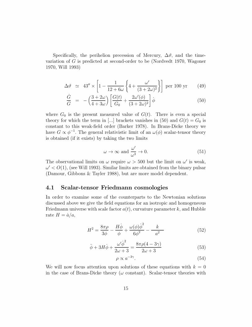
Specifically, the perihelion precession of Mercury, ∆ϑ, and the time-variation of G is predicted at second-order to be (Nordvedt 1970, Wagoner1970, Will 1993)

∆ϑ ≃ 43′′ ×[

1− 1

12 + 6ω

4 +ω′

(3 + 2ω)2

]

per 100 yr (49)

G

G= −

(

3 + 2ω

4 + 3ω

)

[

G(t)

G0+

2ω′(φ)

(3 + 2ω)2

]

φ (50)

where G0 is the present measured value of G(t). There is even a specialtheory for which the term in [...] brackets vanishes in (50) and G(t) = G0 isconstant to this weak-field order (Barker 1978). In Brans-Dicke theory wehave G ∝ φ−1. The general relativistic limit of an ω(φ) scalar-tensor theoryis obtained (if it exists) by taking the two limits

ω → ∞ andω′

ω3→ 0. (51)

The observational limits on ω require ω > 500 but the limit on ω′ is weak,ω′ < O(1), (see Will 1993). Similar limits are obtained from the binary pulsar(Damour, Gibbons & Tayler 1988), but are more model dependent.

4.1 Scalar-tensor Friedmann cosmologies

In order to examine some of the counterparts to the Newtonian solutionsdiscussed above we give the field equations for an isotropic and homogeneousFriedmann universe with scale factor a(t), curvature parameter k, and Hubblerate H = a/a,

H2 =8πρ

3φ− Hφ

φ+ω(φ)φ

2

6φ2 − k

a2(52)

φ+ 3Hφ+ω′φ

2

2ω + 3=

8πρ(4− 3γ)

2ω + 3(53)

ρ ∝ a−3γ . (54)

We will now focus attention upon solutions of these equations with k = 0in the case of Brans-Dicke theory (ω constant). Scalar-tensor theories with

15

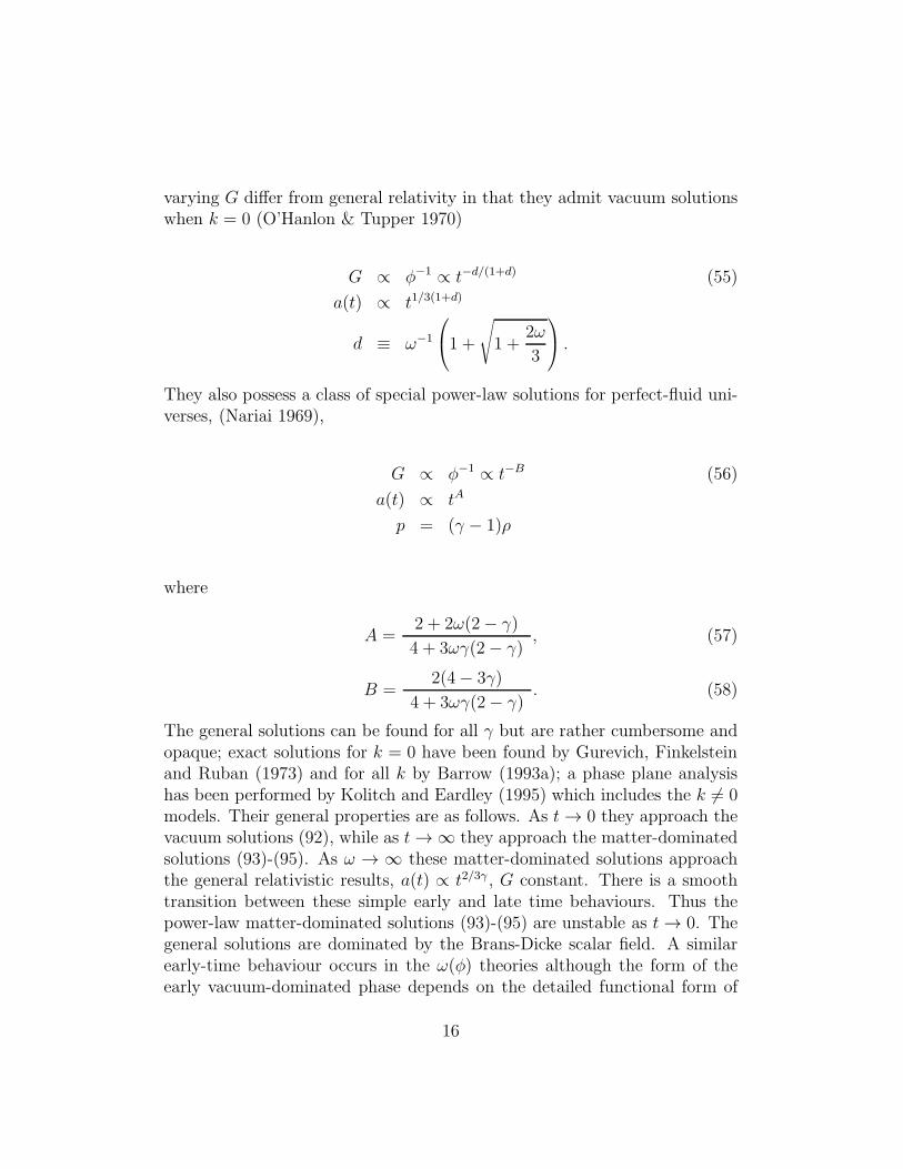
varying G differ from general relativity in that they admit vacuum solutionswhen k = 0 (O’Hanlon & Tupper 1970)

G ∝ φ−1 ∝ t−d/(1+d) (55)

a(t) ∝ t1/3(1+d)

d ≡ ω−1

1 +

√

1 +2ω

3

.

They also possess a class of special power-law solutions for perfect-fluid uni-verses, (Nariai 1969),

G ∝ φ−1 ∝ t−B (56)

a(t) ∝ tA

p = (γ − 1)ρ

where

A =2 + 2ω(2− γ)

4 + 3ωγ(2− γ), (57)

B =2(4− 3γ)

4 + 3ωγ(2− γ). (58)

The general solutions can be found for all γ but are rather cumbersome andopaque; exact solutions for k = 0 have been found by Gurevich, Finkelsteinand Ruban (1973) and for all k by Barrow (1993a); a phase plane analysishas been performed by Kolitch and Eardley (1995) which includes the k 6= 0models. Their general properties are as follows. As t→ 0 they approach thevacuum solutions (92), while as t→ ∞ they approach the matter-dominatedsolutions (93)-(95). As ω → ∞ these matter-dominated solutions approachthe general relativistic results, a(t) ∝ t2/3γ , G constant. There is a smoothtransition between these simple early and late time behaviours. Thus thepower-law matter-dominated solutions (93)-(95) are unstable as t→ 0. Thegeneral solutions are dominated by the Brans-Dicke scalar field. A similarearly-time behaviour occurs in the ω(φ) theories although the form of theearly vacuum-dominated phase depends on the detailed functional form of

16

ω(φ), (see Barrow 1993a, 1993b, Barrow and Mimoso 1994, Damour andNordvedt 1993, Serna and Alimi 1996, and Barrow and Parsons 1996 fordetails).

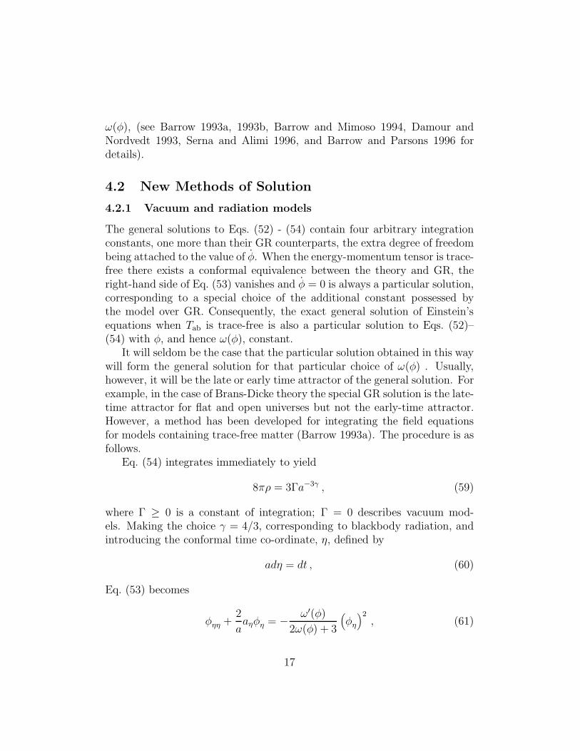
4.2 New Methods of Solution

4.2.1 Vacuum and radiation models

The general solutions to Eqs. (52) - (54) contain four arbitrary integrationconstants, one more than their GR counterparts, the extra degree of freedombeing attached to the value of φ. When the energy-momentum tensor is trace-free there exists a conformal equivalence between the theory and GR, theright-hand side of Eq. (53) vanishes and φ = 0 is always a particular solution,corresponding to a special choice of the additional constant possessed bythe model over GR. Consequently, the exact general solution of Einstein’sequations when Tab is trace-free is also a particular solution to Eqs. (52)–(54) with φ, and hence ω(φ), constant.

It will seldom be the case that the particular solution obtained in this waywill form the general solution for that particular choice of ω(φ) . Usually,however, it will be the late or early time attractor of the general solution. Forexample, in the case of Brans-Dicke theory the special GR solution is the late-time attractor for flat and open universes but not the early-time attractor.However, a method has been developed for integrating the field equationsfor models containing trace-free matter (Barrow 1993a). The procedure is asfollows.

Eq. (54) integrates immediately to yield

8πρ = 3Γa−3γ , (59)

where Γ ≥ 0 is a constant of integration; Γ = 0 describes vacuum mod-els. Making the choice γ = 4/3, corresponding to blackbody radiation, andintroducing the conformal time co-ordinate, η, defined by

adη = dt , (60)

Eq. (53) becomes

φηη +2

aaηφη = − ω′(φ)

2ω(φ) + 3

(

φη

)2, (61)

17

where subscript η denotes a derivative with respect to conformal time. Thisintegrates exactly to give,

φηa2 = 31/2A(2ω(φ) + 3)−1/2 ; A const. (62)

We now employ the variable (suggested by the conformal invariance) usedby Lorenz-Petzold (1984) to study Brans-Dicke models,

y = φa2 , (63)

to re-write the scalar-tensor version of the Friedmann equation, Eq. (52), as

(yη)2 = −4ky2 + 4Γy +

1

3

(

φη

)2a4(2ω(φ) + 3) . (64)

Dividing Eq. (62) by Eq. (63), and using Eq. (62), we obtain the coupledpair of differential equations

φη

φ= 31/2Ay−1(2ω(φ) + 3)−1/2 , (65)

(yη)2 = −4ky2 + 4Γy + A2 . (66)

We may now obtain the general solution for a particular choice of ω(φ), givenk. Integrating Eq. (65) yields y(η) which, in conjunction with ω(φ), impliesφ(η) and, without further integration, a(η) from Eq. (63). If Eq. (60) canbe integrated and inverted we may compute φ(t) and a(t), so completing thesolution. The vacuum models are obtained by setting Γ = 0.

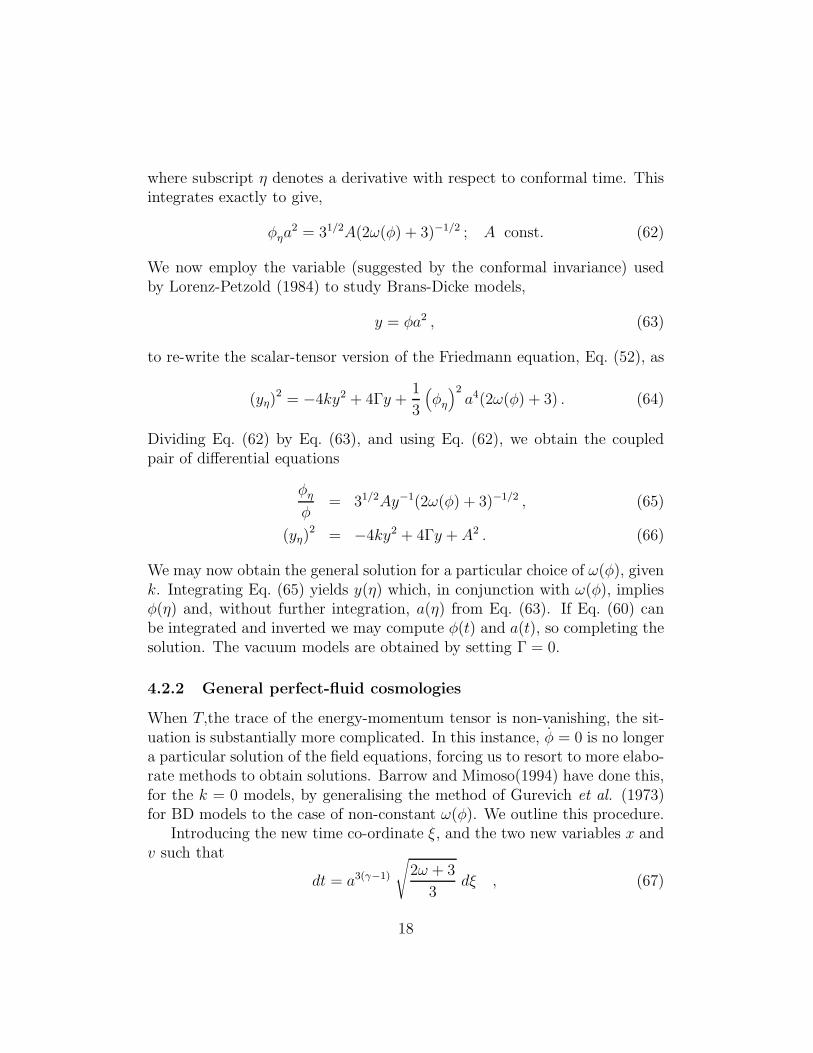
4.2.2 General perfect-fluid cosmologies

When T,the trace of the energy-momentum tensor is non-vanishing, the sit-uation is substantially more complicated. In this instance, φ = 0 is no longera particular solution of the field equations, forcing us to resort to more elabo-rate methods to obtain solutions. Barrow and Mimoso(1994) have done this,for the k = 0 models, by generalising the method of Gurevich et al. (1973)for BD models to the case of non-constant ω(φ). We outline this procedure.

Introducing the new time co-ordinate ξ, and the two new variables x andv such that

dt = a3(γ−1)

√

2ω + 3

3dξ , (67)

18

x ≡[

φa3(1−γ)(

a3)

ξ

]

, (68)

v ≡[

a3(2−γ)φξ

]

, (69)

and confining attention to the k = 0 models, Eqs. (52)-(54) transform to

(

2

3x+ v

)2

=(

2ω + 3

3

)

[

v2 + 4Γφa3(2−γ)]

, (70)

vξ = Γ (4− 3γ) , (71)

and

xξ = 3Γ [(2− γ)ω + 1] +3

2

(

2

3(2ω + 3)x+ v

)

ωξ , (72)

where subscript-ξ represents a derivative with respect to ξ-time. Eqs. (71)and (72) integrate easily to yield

v = Γ(4− 3γ) (ξ − ξ1) , (73)

x =3

2

[

−v +√2ω + 3

(

C + Γ(2− γ)∫ ξ

ξ1

√2ω + 3 dξ

)]

, (74)

C is an integration constant and ξ1 fixes the origin of ξ-time. Noting therelation

3

aφaξφξ =

1

φ2

(

φξ

)23φ

a

aξφξ

=1

φ2

(

φξ)2 x

v, (75)

and differentiating y, with respect to ξ, yields

(

φξ

φ

)

ξ

+

[

3γ − 4

2+

1

ξ − ξ1fξ(ξ)

] (

φξφ

)2

=1

ξ − ξ1

φξ

φ, (76)

where a new function f(ξ), is defined by

f(ξ) ≡∫ ξ

ξ1

3(2− γ)

2Γ(4− 3γ)

√

2ω(φ) + 3

[

C + Γ(2− γ)∫ ξ

ξ1

√

2ω(φ) + 3 dξ

]

dξ .

(77)Solving Eq. (76), we have the solution

ln

(

φ

φ0

)

=∫ ξ

ξ1

ξ − ξ1g(ξ)

dξ , (78)

19

with g(ξ) simply related to f(ξ) by

g(ξ) ≡ f(ξ) +3γ − 4

4(ξ − ξ1)

2 +D , (79)

where D is a constant of integration. Eq. (75) immediately reveals a simpleformula for the scale-factor:

a3 = a30

(

g

φ

)1

2−γ

; a0 constant . (80)

Finally, the scalar-tensor coupling function ω(φ) is given as a function of fby

2ω (φ(ξ)) + 3 =4− 3γ

3(2− γ)2(f ′)2

[

f + 4−3γ3(2−γ)2

f0] , (81)

where f0 is another arbitrary constant.An important benchmark is provided by the behaviour of the BD theory,

where ω(φ) = ω0 = constant. In this case, the generating function, f(ξ), isgiven by a quadratic in ξ:

fBD(ξ) =3(2− γ)

2Γ(4− 3γ)

√2ω0 + 3

[

C ξ +Γ(2− γ)

2ξ2

√2ω0 + 3

]

. (82)

Hence, in general (C 6= 0 6= Γ) when γ 6= 4/3 , 2, we see that fBD ∝ ξ2

as ξ → ∞ and fBD ∝ ξ as ξ → 0, where dt ∝ a3(γ−1)dξ. If we chooseC = 0 then fBD ∝ Γξ2 as ξ → 0. The choice C = 0 restricts the solutionto the special ‘matter-dominated’ solutions (termed ‘Machian’ by Dicke, seeWeinberg (1972)) which were first found for all perfect-fluids by Nariai (1969).If C 6= 0 then the early-time behaviour is dominated by the dynamics of theφ-field; such solutions are termed ‘φ-dominated’ (or ‘non-Machian’ by Dicke).

Therefore if we choose a generating function g(ξ) that grows slower thanξ2 as ξ → ∞ it will produce a theory that approaches BD at late times(φ →constant, ω(φ) → constant), whilst if g(ξ) decreases slower than ξ asξ → 0 then the theory will approach the behaviour of φ-dominated BDtheory at early-times. This means that we will find new (non-BD) late-time behaviours by studying generating functions which increase faster thang(ξ) = ξ2 as ξ → ∞ and new (non-BD) early-time behaviour by pickinggenerating functions which decrease slower than g(ξ) = ξ as ξ → 0 or ξ →ξmin (if there is no zero of ξ at the minimum of a(t)).

20

4.3 Comparing Newtonian and Relativistic Cosmolo-

gies

It is now possible to consider some of the similarities and differences thatexist between the Newtonian cosmologies with varying G and their curvedspace-time counterparts. We recall that the special Newtonian power-lawsolutions (24) have the form G ∝ t−n with scale factor r ∝ t(2−n)/3γ . This isidentical to the Brans-Dicke solution when p = 0 and

n =2

4 + 3ω. (83)

In fact, for any choice of ω(φ) dust universes have

φa3 → t2 (84)

which corresponds to Newtonian solutions with G ∝ t−n and scale factorr ∝ t(2−n)/3 .

The vacuum solutions have a slightly different structure. If we identify

n =d

d+ 1(85)

then we have

a(t) ∝ t1/3(1+d) ∝ t(1−n)/3. (86)

However, there is no general correspondence for other equations of state.Most notably, Brans-Dicke radiation-dominated universes (γ = 4/3) are thesame as in general relativity, G = constant and a(t) ∝ t1/2, and differ fromthe radiation solutions. In general, the Newtonian solutions are the same asthe Brans-Dicke matter-dominated solutions only if we make the choice

n =2(4− 3γ)

4 + 3ωγ(2− γ). (87)

Also, as can be seen from the right-hand side of the φ(t) evolution equa-tion, (90), the effective sign of the gravitational coupling changes sign fromnegative to positive when γ becomes greater than 4/3.

The Newtonian inflationary solutions with γ = 0, given in eqn. (29), donot have direct counterparts in Brans-Dicke gravity theories. However, scalartensor theories with

21

2ω + 3 ∝ φh (88)

have solutions of similar form as t → ∞ with (Barrow and Mimoso 1994,Barrow and Parsons 1996)

G ∝ φ−1 ∝ t−2/(2h+1) (89)

and the scale factor evolves as

a(t) ∝ t(h−1)/3(2h+1) exp

At2h/(2h+1)

. (90)

Thus, with 2h + 1 > 0, we have ω → ∞ and ω′/ω3 → 0 as t → ∞and general relativity is approached in the weak-field limit. These solutionsare not of identical form to the Newtonian solutions with G ∝ t−n andn = 2/(2h+ 1).

5 Gravitational memory

The process of primordial black hole formation in a cosmological model withvarying G creates an interesting problem. We know (Hawking 1972) thatblack holes in scalar-tensor gravity theories are identical to those occurringin general relativity. Suppose, for simplicity, that a Schwarzschild black holeforms in the very early universe at a time tf when the gravitational couplingG(tf) differs from the value G(t0) that we observe at the present cosmictime, t0. This black hole will have an horizon size Rf = 2G(tf)M ∼ tfwhen it forms. We now ask what happens to this black hole during thesubsequent evolution of the universe as the value of G changes with time inthe background universe (Barrow 1992, Barrow and Carr 1996).

There appear to be two alternatives. The value of G(t) on the scale ofthe even horizon could change at the same rate as that in the backgrounduniverse. But this would imply that the black hole was changing with time.Thus it could not be one of the black holes defined in general relativity, asrequired. Moreover, if G < 0,the horizon area (Ahor) would decrease withtime and so would the associated entropy which is given by (Kang 1996)

Sbh =Ahor × φhor

4

22

where φhor = G−1hor determines the value of G on the horizon. Alternatively,

there might be a process of ’gravitational memory’ (Barrow 1992) whereinthe scalar field determining G remains constant on the scale of the blackhole horizon whilst changing in the cosmological background. That is atany moment of cosmic time there would be a space variation in G. Thishas dramatic implications for the Hawking evaporation of primordial blackholes. For the lifetime and temperature of an evaporating black hole will bedetermined by the value of G(tf) at the time when it formed rather than bythe value G(t0) we observe in the universe today: the black hole ’remembers’the value of G at the time of its formation. Hence, its Hawking lifetime willbe τ bh ∼ G2

fM3 and its temperature Tbh ∼ G−1

f M−1.Black holes which explode today are those whose Hawking lifetime is

equal to the present age of the universe. This fixes their masses to be

Mex ≃ 4× 1014 ×(

G(t0)

G(tf)

) 2

3

gm

and their temperature when the explode is therefore given by

Tex ≃ 24×(

G(t0)

G(tf)

)1

3

MeV.

Clearly, if there has been significant change in the value of G sincetf ∼ 10−23s then the physical characteristics of exploding black holes canbe very different from those predicted under the assumption that G doesnot change (Hawking 1974). Quite modest amounts of time evolution atunobservably early times can shift the spectral range in which we would seethe evaporation products out of the gamma-ray band. This means that weshould be looking for the evidence of black hole evaporation in other partsof the electromagnetic spectrum. A more detailed study of the observationalevidence, seen is this light, is given by Barrow and Carr (1996).

6 Origins of the Values of Constants

In recent years there has been a good deal of speculation about mechanismsfor explaining the values of the fundamental constants. At one time it waswidely believed that some ultimate Theory of Everything would eventually

23

tell us that the constants could have one, and only one, set of logically self-consistent values. Such a simple scenario now seems less and less likely (Bar-row 1991). There are so many sources of randomness in the process whichendow the fundamental constants with their low-energy values, and the pa-rameters likely to be fixed by a Theory of Everything are so far removed fromour three-dimensional physical constants, that many new possibilities mustbe taken seriously. The non-uniqueness of the ground state of any Theoryof Everything would mean that fundamental constants could take on manyself-consistent sets of values. We would have to use anthropic constraintsin order to understand those that we observe. This creates new interpreta-tional problems. Our underlying Theory of Everything would have quantumgravitational characteristics and its predictions about constants would havea probabilistic form. Although, formally, there would be a most probablevalue for the low-energy measurement of a quantity like the fine structureconstant, such a value might be irrelevant for observational purposes (Bar-row 1994). We would only be interested in the range of values for which theevolution of complexity, in the form that we call ’life’, is possible. This maywell confine us to a subset of values which, a priori, is extremely improbable.This shows that in order to make a correct comparison of the probabilisticpredictions of such a theory with observation we would need to know everydependence of processes which can lead to the evolution of complexity on thevalues of the constants of Nature.

The fact that the observed values of many of the constants of Nature fallwithin a very narrow range for which life appears to be possible has eliciteda variety of interpretations:

(i) Good luck: the constants are what they are and could be no otherway. The range which allows intelligent observers to evolve and persist isnarrow and we are very lucky that our universe falls within that range. Nomatter how improbable this sate of affairs we could observe it to be no otherway.

(ii) Life is inevitable: we have been misled by our limited knowledge ofcomplexity into thinking that life is restricted to universes spanned by a verynarrow range of values for the constants. In fact, life may be a widespreadinevitability in the phase space of all possible values of the constants. Evenour own form of carbon-based life may exist in other novel forms which ex-ploit the possibilities provided by the recently discovered fullerene chemistry.complexity of the sort that we call life may also exist in quite different formsto those we are accustomed to: for example, existing in velocity space rather

24

than in position space.(iii)All possibilities exist: whether through the actualisation of quantum-

mechanical many-worlds, the realisation of all logically consistent Theoriesof Everything, or some elaboration of the self-reproducing universe scenar-ios, every possible permutation of the values of the constants exists in someuniverse. We live in one of the subset which allows life to exist. It is alsopossible that the ensemble of possibilities is played out in a single infiniteUniverse and we inhabit one of the life-supporting parts of it.

(iv) Cosmic fine tuning: some physical process brings about approachto a particular set of values for the constants over long periods of time,perhaps through many cycles of cosmic evolution. The attracting set may bepredictable in certain respects.

The last of these four possibilities has attracted some interest recently.Harrison (1995) made the amusing suggestion that the fine tuning of theconstants may be the end result of successive intelligent interventions bybeings able to create universes in the laboratory (something discussed inthe literature even by ourselves! Farhi and Guth (1987)).Aware that cer-tain combinations of the values of fundamental constants raise the probabil-ity of life evolving, and able to engineer these values at inception, succes-sive generations would tend to find themselves inhabiting universes in whichlife-supporting combinations obtained to high precision. Although Harrisonrefers to his as a ’natural selection’ of universes, it is more akin to artificialselection, or forced breeding.

Linde (1990) has proposed generalisations of the self-reproducing eternalinflationary universe in which the values of the fundamental constants changefrom generation to generation. Although unobservable, this scheme has themerit of being a by-product of the standard chaotic inflationary universescenario.

A third scenario of this sort, which has attracted a surprising amount ofattention is that proposed by Smolin (1992) who suggested that a bounce,or quantum tunnelling, occurs at all final black-hole-collapse singularitieswhich transforms them into initial singularities for new expanding universes.During this process the constants of Nature undergo small random changes.It is expected therefore that selection pressure will act so as to maximise theblack holes produced in universes as time goes on (no weighting of the volumetaking part in this reproduction process is introduced though, as is the casein the self-reproducing inflationary universes). Thus, if our universe is theresult of the action of this selection process over many cycles of collapse

25

and re-expansion, in which the constants have lost memory of any initialconditions they may have had, then Smolin argues that we would expectto be near a local maximum in the black-hole production. Hence, small

changes in the constants of Nature should in general take us downhill fromthis local maximum and always reduce the amount of black hole production.By conducting such thought-experiments the general consistency of the ideacan be tested.

We make three remarks about this speculative scenario. First, it is notclear that is as sharply predictive and testable as claimed. We should only ex-pect to find ourselves residing near a local maximum in the space of constantsif that maximum also provides conditions which permit living observers toexist. If those condition are unusual then we might have to exist in one ofthe improbable universes far from the local maxima. We can only deter-mine if this is the case by having a complete understanding of the necessaryand sufficient conditions for living complexity to exist. Second, putting thisobjection to one side, there may well be small changes in the values of the con-stants which significantly increase the production of black holes. For exam-ple a small (70KeV ) strengthening of the strong interaction would bind thedineutron and the diproton (helium-2), so providing a direct H +H → He2

channel for nuclear burning. massive stars would run through their evolu-tion very rapidly and end as black holes far sooner and with higher likelihoodthan at present (see Dyson 1971, Barrow 1987). Third, we might ask whythere should be any local maxima at all for variations in certain constants.Variation would proceed to states of higher gravitational entropy by alwaysincreasing the value of Sbh ∝ GM2, and this would be effected by a randomwalk upwards through (over long time averaged) increasing values of G.

Finally, we should note that any scheme which relies upon random changesin the constants of Nature occurring at the endpoint of gravitational collapsemust beware of the consequences of changes which prevent future collapsesfrom occurring. A specific example is seen in the case of closed universesoscillating under the requirement that their total entropy increase from cycleto cycle. There, one finds that any positive cosmological constant (no matterhow small in value) which remains constant (or falls slowly enough on aver-age) from cycle to cycle ultimately stops the sequence of growing oscillationsand leaves the Universe in a state of indefinite expansion which asymptotestowards the de Sitter state (Barrow and Dabrowski 1995). In Smolin’s sce-nario one might consider that if the curvature of space or the value of thecosmological constant, or the magnitude of vacuum stresses associated with

26

scalar fields which violate the strong energy condition, were to change at thecollapse event in ways that prevented future collapse of some or all of theUniverse, then gradually the fraction of the Universe which could gravitation-ally collapse and evolve the values of its constants by random reprocessingwould shrink asymptotically to zero. Evolution would cease. This Universewould have ’died’.

7 Simultaneous Variations of Many Constants

The subject of varying constants is of particular current interest becauseof the new possibilities opened up by the structure of unified theories, likestring theory and M-theory, which lead us to expect that additional compactdimensions of space may exist. Although these theories do not require tradi-tional constants to vary, they allow a rigorous description of any variations tobe provided: one which does not merely ‘write in’ the variation of constantsinto formulae derived under the assumption that they do not vary. This self-consistency is possible because of the presence of extra dimensions of spacein these theories. The ‘constants’ seen in a three-dimensional subspace ofthe theory will vary at the same rate as any change occurring in the extracompact dimensions. In this way, consistent simultaneous variations of dif-ferent constants can be described and searches for varying constants providea possible observational handle on the question of whether extra dimensionsexist (Marciano, 1984, Barrow 1987, Damour & Polyakov 1994).

Prior to the advent of theories of this sort, only the time variation ofthe gravitational constant could be consistently described using scalar-tensorgravity theories, of which the Brans-Dicke theory is the simplest example.The modelling of variations in other ‘constants’ was invariably carried out byassuming that the time variation of a constant quantity, like the fine structureconstant, could just be written into the usual formulae that hold when it isconstant. One way of avoiding this situation is to exploit the invarianceproperties of the non-relativistic Schrodinger equation for atomic structure,which allow it to be written in dimensionless form when atomic (’Hartree’)units are chosen. It can be shown (Barrow and Tipler 1986) that any solutionwith an energy eigenvalue E, arising when the fine structure constant is αand the electron mass is me,must be related to a solution defined by a E, α′,and m

′

e by the relation

27

E

α2mec2=

E ′

α′2m′ec

2(91)

where c is the velocity of light.The possibility of linked variations in low-energy constants as a result

of high-energy unification schemes has the added attraction of providing amore powerful means of testing those theories (Marciano 1984, Kolb, Perry,& Walker, 1986, Barrow 1987, Dixit & Sher 1988, Campbell & Olive 1995).

Higher-dimensional theories typically give rise to relationships of the fol-lowing sort

αi(m∗) = AiGm2∗= Biλ

n(ℓpl/R)k;n, k constants (92)

α−1i (µ) = α−1

i (m∗)−π−1

∑

Cij [ln(m∗/mj) + θ(µ−mj) ln(mj/µ)] + ∆i

where αi(..) are the three gauge couplings evaluated at the correspondingmass scale; µ is an arbitrary reference mass scale, m∗ is a characteristicmass scale defining the theory (for example, the string scale in a heteroticstring theory); λ is some dimensionless string coupling; ℓpl = G−1/2 is thePlanck length, and R is a characteristic mean radius of the compact extra-dimensional manifold; Cij are numbers defined by the particular theoriesand the constants Ai and Bi depend upon the topology of the additional( > 3) dimensions. The sum is over j = leptons, quarks, gluons, W±, Zand applies at energies above µ ∼ 1GeV (Marciano 1984). The term ∆i

corresponds to some collection of string threshold corrections that arise inparticular string theories or an over-arching M theory (Antoniadis & Quiros1996). They contain geometrical and topological factors which are specifiedby the choice of theory. By differentiating these two expressions with respectto time (or space), it is possible to determine the range of self-consistentvariations that are allowed. In general, for a wide range of super-symmetricunified theories, the time variation of different low-energy constants will belinked by a relationship of the form (where we consider β to denote the timederivative of β etc.)

δ0β

β= δ1

G

G+∑

δ2iαi

α2i

+ δ3m∗

m∗

+∑

δ4jmj

mj+ δ5

λ

λ+ ... (93)

where β ≡ me/mpr (Drinkwater et al 1997). It is natural to expect that allthe terms involving time derivatives of ‘constants’ will appear in this relation

28

unless the constant δ prefactors vanish because of supersymmetry or someother special symmetry of the underlying theory. This relation shows that,since we might expect all terms to be of similar order (although there maybe vanishing constant δ prefactors in particular theories), we might expectvariations in the Newtonian gravitational ‘constant’, G/G, to be of orderα/α2.

8 Varying alpha – New Observational Limits

Quasar absorption systems present ideal laboratories in which to search forany temporal or spatial variation in the assumed fundamental constants ofNature. Such ideas date back to the 1930s, with the first constraints fromspectroscopy of QSO absorption systems arising in the 1960s. An historicalsummary of the various propositions is given in Varshalovich & Potekhin(1995) and further discussion of their theoretical consequences is given inBarrow & Tipler (1986).

Recently, we have considered the bounds that can be placed on the varia-tion of the fine structure constant and proton g factor from radio observationsof atomic and molecular transitions in high redshift quasars (Drinkwater etal 1997). To do this we exploited the recent dramatic increase in quality ofspectroscopic molecular absorption at radio frequencies, of gas clouds at in-termediate redshift, seen against background radio-loud quasars. Elsewhere,we will consider the implications of simultaneous variations of several ‘con-stants’ and show how these observational limits can be used to constraina class of inflationary universe theories in which small fluctuations in thefine-structure constant are predicted to occur.

The rotational transition frequencies of diatomic molecules such as CO areproportional to h/(Ma2) where M is the reduced mass and a = h2/(mee

2) isthe Bohr radius. The 21 cm hyperfine transition in hydrogen has a frequencyproportional to µpµB/(ha

3), where µp = gpeh/(4mpc), gp is the proton g-factor and µB = eh/(2mec). Consequently (assuming mp/M is constant)the ratio of a hyperfine frequency to a molecular rotational frequency isproportional to gpα

2 where α = e2/(hc) is the fine structure constant. Anyvariation in y ≡ gpα

2 would therefore be observed as a difference in theapparent redshifts: ∆z/(1 + z) ≈ ∆y/y. Redshifted molecular emission ishard to detect but absorption can be detected to quite high redshifts (seereview by Combes & Wiklind, 1996). Recent measurements of molecular

29

absorption in some radio sources corresponding to known HI 21 cm absorptionsystems give us the necessary combination to measure this ratio at differentepochs.

Common molecular and HI 21 cm absorptions in the radio source PKS1413+135 have previously been studied by Varshalovich & Potekhin (1996).They reported a difference in the redshifts of the CO molecular and HI 21 cmatomic absorptions which they interpreted as a mass change of ∆M/M =(−4 ± 6) × 10−5 but as we show above this comparison actually constrainsgpα

2, not mass. Furthermore they used overestimates of both the valueand error. They used the Wiklind & Combes (1994) measurement whichhad the CO line offset from the HI velocity by −11 kms−1; a corrected COmeasurement (Combes & Wiklind, 1996) shows there is no measurable offset.Furthermore, Varshalovich & Potekhin (1996) used the width of the HI linefor the measurement uncertainty. Even allowing for systematic errors the trueuncertainty is at least a factor of 10 smaller so these data in fact establish alimit of order 10−5 or better. This potential for improved limits has promptedthe present investigation: previous upper limits on change in α are of order∆α/α ≈ 10−4 (Cowie & Songalia, 1995; Varshalovich, Panchuk & Ivanchik,1996).

8.1 Comparison of HI and molecular systems

Our new more accurate redshift estimates (Drinkwater et al 1997) give amolecular redshift of 0.684680±0.000006 and an a 21cm redshift of 0.684684±0.000006 for the source 0218 + 357 and a molecular redshift of 0.246710 ±0.000005 and a 21cm redshift of 0.246710±0.000004 for the source 1413+135.We can therefore combine the uncertainties in quadrature to give 1-sigmaupper limits on the redshift differences. These give |∆z/1 + z| < 5 × 10−6

(1.5 kms−1) for both sources.We must still consider the possibility that the molecular and atomic ab-

sorption arises in different gas clouds along the line of sight. This couldexplain any observed difference. However there is no measurable differencebetween the two velocities in our data, so we are probably detecting the samegas. The alternative would be that there was a change in the frequencies butthat in both cases it was exactly balanced by the random relative velocity ofthe two gas clouds observed. We consider this very unlikely because of thesmall 1Kms−1 dispersion within single clouds.

We can now use the limits to ∆z/1 + z with the relationship to derive

30

1-sigma limits on any change in y = gpα2: |∆y/y| < 5×10−6 at both z = 0.25

and z = 0.68. These are significantly lower than the previous best limit of1 × 10−4 by Varshalovich & Potekhin (1996) (it was quoted as a limit onnucleon mass, but it actually refers to gpα

2).As there are no theoretical grounds to expect that the changes in gp and

α2 are inversely proportional, we obtain independent rate-of-change limits of|gp/gp| < 2 × 10−15 y−1 and |α/α| < 1× 10−15 y−1 at z = 0.25 and |gp/gp| <1×10−15 y−1 and |α/α| < 5×10−16 y−1 at z = 0.68 (forH0 = 75 kms−1 Mpc−1

and q0 = 0 assumed here). These new limits are stronger than the previous1 sigma limit of |α/α| < 8× 10−15 y−1 at z ≈ 3 (Varshalovich et al. 1996).

The most stringent laboratory bound on the time variation of α comesfrom a comparison of hyperfine transitions in Hydrogen and Mercury atoms(Prestage et al. 1995), |α/α| < 3.7 × 10−14y−1, and is significantly weakerthan our astronomical limit. The other strong terrestrial limit that we haveon time variation in α comes from the analysis of the Oklo natural reactorat the present site of an open-pit Uranium mine in Gabon, West Africa.A distinctive thermal neutron capture resonance must have been in place1.8 billion years ago when a combination of fortuitous geological conditionsenriched the subterranean Uranium-235 and water concentrations to levelsthat enabled spontaneous nuclear chain reactions to occur (Maurette 1972).Shlyakhter (1976, 1983) used this evidence to conclude that the neutronresonance could not have shifted from its present specification by more than5 × 10−4eV over the last 1.8 billion years and, assuming a simple model forthe dependence of this energy level on coupling constants like α, derived alimit in the range of |α/α| < (0.5–1.0) × 10−17y−1. The chain of reasoningleading to this very strong bound is long, and involves many assumptionsabout the local conditions at the time when the natural reactor ran, togetherwith modelling of the effects of any variations in electromagnetic, weak, andstrong couplings. Recently, Damour & Dyson (1997) have provided a detailedreanalysis in order to place this limit on a more secure foundation. Theyweaken Shlyakhter’s limits slightly but give a 95% confidence limit of −6.7×10−17y−1 < α/α < 5.0 × 10−17y−1. However, if there exist simultaneousvariations in the electron-proton mass ratio this limit can be weakened.

These limits provide stronger limits on the time variation of α than theastronomical limits; however, the astronomical limits have the distinct advan-tage of resting upon a very short chain of theoretical deduction and are moreclosely linked to repeatable precision measurements of a simple environment.The Oklo environment is sufficiently complex for significant uncertainties to

31

remain.Unlike the Oklo limits, the astronomical limits also allow us to derive up-

per limits on any spatial variation in α. Spatial variation is expected from thetheoretical result that the values of the constants would depend on local con-ditions and that they would therefore vary in both time and space (Damour& Polyakov 1994). The two sources for which we derived limits, 0218+357and 1413+135, are separated by 131 degrees on the sky, so together with theterrestrial result, we find the same values of α to within |∆α/α| < 3 × 10−6

in three distinct regions of the universe separated by comoving separationsup to 3000Mpc. Limits on spatial variation of gpα

2me/mp were previouslydiscussed by Pagel (1977, 1983) and Tubbs & Wolfe (1980). We have im-proved on their limits by some 2 orders of magnitude but as our sources areat lower redshift, they are not causally disjoint from each other.

The high-redshift measurements are now approaching the best terrestrialmeasurements based on the Oklo data. These could be further improvedby a factor of 2–5 with additional observations that would not be difficultto perform such as fitting the atomic and molecular data simultaneously,remeasuring the HI absorptions at higher spectral resolution.

8.2 Inflation

Inflation is something of a two-edged sword when it comes to discussingvariations in constants. On the one hand there are potentials with multiplevacuum states which allow different parts of the universe to find themselvesinheriting different suites of fundamental constants, with quite different val-ues. On the other hand, if, as inflation leads us to expect, the whole ofour observable universe is contained within the inflated image of a singlecausally connected region, then we should expect fundamental constants toreflect that single origin and to display spatial uniformity to very high pre-cision. The key question is what precisely is that precision? A bench markfor the amplitude of possible variations is provided by the amplitude of tem-perature fluctuations in the microwave background, ∆T/T ≃ 10−5. Wewould expect fluctuations in the fine structure constant created at the endof inflation to have an almost constant curvature spectrum (because of thetime-translation invariance of almost de Sitter inflation) with an amplitudebelow that of 10−5. An interesting feature of the new astronomical observa-tions described above is that, for the first time, they take the observationallimits on spatial variations in α ( |∆α/α| < 3×10−6) into that regime where

32

they may be constraining the underlying theories more strongly than are theCOBE observations.

Acknowledgements

The author acknowledges support by a PPARC Senior Fellowship. Someof the work described here was carried out in collaboration with BernardCarr, Michael Drinkwater, Victor Flambaum, Jose Mimoso, Paul Parsonsand John Webb. I am most grateful to them for their contributions. Iwould also like to thank Norma Sanchez for her encouragement and heradministrative assistants in Erice for their assistance in Erice.

References

Antoniadis I., Quiros M., 1996, Large Radii and String Unification, preprint.Barker B.M., 1978, Ap. J., 219, 5Barrow J.D., 1987, Phys. Rev., D 35, 1805Barrow J.D., 1990a, in Modern Cosmology in Retrospect, eds., Bertotti

B., Balbinot R., Bergia S., Messina A., pp67-93, Cambridge UP, CambridgeBarrow J.D., 1990b, Phys. Lett., B235, 40Barrow J.D., 1991, Theories of Everything, Oxford UP, Oxford.Barrow J.D., 1992, Phys. Rev. D 46, R3227Barrow J.D., 1993a, Phys. Rev., D 47, 5329Barrow J.D., 1993b, Phys. Rev., D 48, 3592Barrow J.D., 1994, The Origin of the Universe, Basic Books, NY.Barrow J.D., 1995, Phys. Rev., D 51, 2729Barrow J.D., 1996, MNRAS 282, 1397Barrow J.D., Carr B.J., 1996, Phys. Rev. D54, 3920.Barrow J.D., Dabrowski M.P.,1995 MNRAS 275, 850Barrow J.D., Gotz G., 1989a, Class. Quantum Gravity, 6, 1253Barrow J.D., Liddle A.R., 1993, Phys. Rev., D 47, R5219Barrow J.D., Maeda K., 1990, Nucl. Phys. B341, 294Barrow J.D., Mimoso J.P., 1994, Phys. Rev., D 50, 3746Barrow J.D., Parsons P., 1996, Phys. Rev., D 000,000Barrow J.D., Saich P., 1990, Phys. Lett. B 249, 406Barrow J.D., Tipler F.J., 1986, The Anthropic Cosmological Principle,

Oxford UP, OxfordBatyrev A.A., 1941, Astron. Zh. 18, 343Batyrev A.A., 1949, Astron. Zh. 26, 56Bekenstein J.D., Meisels A., 1980, Phys. Rev., D 22, 1313Bekenstein J.D., Milgrom M., 1984, Ap. J., 286, 7Bekenstein J.D., Sanders R.J., 1994, Ap. J., 429, 480

33

Bergmann P.G., 1968, Int. J. Theo. Phys., 1, 25Brans C., Dicke R.H., 1961, Phys. Rev., 24, 925Callan C.G., Friedan D., Martinec E.J., Perry, M.J., 1985, Nucl. Phys.,

B262, 597Campbell B.A., Olive, K.A., 1995, Phys.Lett. B, 345, 429Cesari L., 1963, Asymptotic Behavior and Stability Problems in Ordinary

Differential Equations, 2nd. edn., Springer-Verlag, BerlinChandrasekhar S., 1937, Nature, 139, 757Combes, F., Wiklind, T., 1996, in Cold Gas at High Redshift, eds. M.Bremer,

P. van der Werf, H. Rottgering, and C. Carilli, Kluwer: Dordrecht, p. 215Cowie L.L., Songalia A., 1995, ApJ, 453, 596Damour, T., Gibbons G.W., Taylor J.H., 1988, Phys. Rev. Lett., 61,

1151Damour T., Nordtvedt K., 1993, Phys. Rev., D 48, 3436Damour T., Dyson F., 1997, Nucl. Phys. B, 480, 37Damour T., Polyakov A.M., 1994, Nucl. Phys. B, 423, 596Davidson W., Evans A.B., 1973, Int. J. Theo. Phys., 7, 353Davidson W., Evans A.B., 1977, Comm. Roy. Soc. Edin. (Phys. Sci.),

10, 123Dicke R.H., 1957, Rev. Mod. Phys. 29, 355Dicke R.H., 1964, in Relativity, Groups and Topology, eds. De Witt C.,

De Witt B., pp. 163-313, Gordon & Breach, New YorkDirac P.A.M., 1937a, Nature, 139, 323Dirac P.A.M., 1937b, Nature, 139, 1001Dirac P.A.M., 1938, Proc. Roy. Soc., A 165, 199Dixit V.V., Sher, M., 1988, Phys.Rev.D, 37, 1097Drinkwater M., Webb J., Barrow J.D., Flambaum V., 1997, MNRAS (in

press)Duval C., Gibbons G., Horvathy P., 1991, Phys. Rev., D 43, 3907Dyson, F., 1971, Sci. American (Sept.) 225, 25Eddington A.S., 1923, The Mathematical Theory of Relativity, Cambridge

UP, London.Evans A.B., 1974, Nature, 252, 109Evans A.B., 1978, MNRAS, 183, 727Farhi E., Guth A., 1987, Phys. Lett. B 183, 149Fischbach E., et al, 1986, Phys. Rev. Lett., 56, 3Freund P.G.O., 1982, Nucl. Phys., B209, 146Gamow G., 1967a, Phys. Rev. Lett., 19, 759

34

Gamow G., 1967b, Phys. Rev. Lett., 19, 913Garcia Bellido J., Linde A., Linde D., 1994, Phys. Rev., D 50, 730Garcia-Berro E., Hernanz M., Isern J., Mochkovitch R., 1995, MNRAS,

277, 801Green M., Schwarz J.H., 1984, Phys. Lett., B149, 117Gurevich L.E., Finkelstein A.M., Ruban V.A., 1973, Astrophys. Sp. Sci.

22, 231Guth A.H., 1981, Phys. Rev., D23, 347Harrison, E.R., 1995, QJRAS 36, 193Hawking S.W., 1972 Commun. Math. Phys. 25, 167 (1972)Hawking S.W. 1974 Nature 248, 30Heckmann O., Schucking E., 1955, Z. Astrophysik, 38, 95Heckmann O., Schucking E., 1959, Handbuch der Physik 53, 489Hellings R.W., 1984, in General Relativity and Gravitation, eds. Bertotti

B., de Felice F., Pascolini A., Reidel, DordrechtHolman R., Kolb E.W., Vadas S., Wang Y., 1991, Phys. Rev., D 43, 3833Jordan P., 1938, Naturwiss., 26, 417Jordan P., 1952, Schwerkraft und Weltall, Grundlagen der Theor. Kos-

mologie, Braunschweig, Vieweg and SohnKang G, 1996, Phys. Rev. D 54, 7483Kolb E.W., Perry M.J., Walker T.P., 1986, Phys. Rev., D 33, 869Kothari D.S., 1938, Nature, 142, 354Kolitch S.J., Eardley D.M., 1995, Ann. Phys. (NY), 241, 128Krauss L.M., White M., 1992, Ap. J., 394, 385La D., Steinhardt P.J., 1989, Phys. Rev. Lett., 62, 376Linde, A., 1990, Inflation and Quantum Cosmology, Academic Press, NYLorentz-Petzold D., 1984, Astrophys. Sp. Sci., 98, 249Lynden-Bell D., 1982 Observatory 102, 86Marciano W.J., 1984, Phys. Rev. Lett., 52, 489Maurette M., 1972, Ann. Rev. Nuc. Part. Sci. 26, 319Mathiazhagen C., Johri V.B., 1984, Class. Quantum Gravity, 1, L29McVittie G.C., 1978, MNRAS, 183, 749Meshcherskii I.V., 1893, Astron. Nach., 132, 129Meshcherskii I.V., 1949, Works in the Mechanics of Bodies of Variable

Mass, Moscow-Leningrad Publ. House, MoscowMilgrom M., 1983, Ap. J., 270, 365Milne E., McCrea W.H., 1934, Quart. J. Math., 5, 73Nariai H., 1969, Prog. Theo. Phys. 42, 544

35

Narlikar J.V., 1963, MNRAS, 126, 203Narlikar J.V., Kembhavi A.K., 1980, Fund. Cosmic Phys., 6, 1Nordvedt K., 1968, Phys. Rev. D169, 1017O’Hanlon J., Tupper B.O.J., 1970, Nuovo Cim. 137, 305Pagel B.E.J., 1977, MNRAS 179, 81PPagel B.E.J., 1983, Phil. Trans. Roy. Soc. A, 310, 245Prestage J.D., Tjoelker R.L., Maleki, L., 1995, Phys. Rev. Lett., 74, 3511Reasenberg R.D., 1983, Phil. Trans. Roy. Soc. Lond., A310, 227Savedoff M.P., Vila S., 1964, AJ 69, 242Serna A., Alimi J.M., 1996, Meudon preprint ’Scalar Tensor Cosmological

Models’Shapiro I., 1990, in General Relativity and Gravitation, eds. Ashby N.,

Bartlett D., Wyss W., Cambridge UP, CambridgeShikin I.S., 1971, Sov. Phys. JETP, 32, 101Shikin I.S., 1972, Sov. Phys. JETP, 34, 236Shlyakhter A.I., 1976, Nature 264, 340Shlyakhter A.I., 1983, Direct test of the time-independence of fundamen-

tal nuclear constants using the Oklo natural reactor, ATOMKI Report A/1Smolin, L., 1992, Classical and Quantum Gravity 9, 173Steinhardt P.J., Accetta F.S., 1990, Phys. Rev. Lett., 64, 2740Teller E., 1948, Phys. Rev., 73, 801Tubbs A.D., Wolfe A.M., 1980, ApJ, 236, L105Varshalovich D. A., Potekhin A. Y., 1995, Space Science Review, 74, 259Varshalovich D. A., Potekhin A. Y., 1996, Pis’ma Astron. Zh., 22, 3Varshalovich D.A., Panchuk V.E., Ivanchik A.V., 1996, Astron. Lett.,

22, 6Vila S.C., 1976, ApJ., 206, 213Vinti J.P., 1974, MNRAS, 169, 417Wagoner R.V., 1970, Phys. Rev., D 1, 3209Weinberg, S.,1972, Gravitation and Cosmology, Wiley, NYWeyl H., 1919, Ann. Physik, 59, 129Wiklind T., Combes F., 1994, A&A, 286, L9Wiklind T., Combes F., 1996, A&A, 315, 86Will C.M., 1993, Theory and Experiment in Gravitational Physics, 2nd

edn., Cambridge UP, CambridgeZwicky F., 1939, Phys. Rev., 55, 726

36