askari-nasab h. & awuah-offei k. 106- 1 106 open pit

Askari-Nasab H. & Awuah-Offei K. 106- 1

106

Open pit optimisation using discounted economic block values

Hooman Askari-Nasab and Kwame Awuah-Offei1 Mining Optimization Laboratory (MOL) University of Alberta, Edmonton, Canada

Abstract

Strategic mine planning and the management of the future cash flows are a vital core of surface mining operations. The time dimension, which is an integral part of the scheduling problem, is not embedded in traditional ultimate pit outline optimisation algorithms. This study explores the validity of the theorem that a pit outline determined by an optimal long-term schedule algorithm is constrained by the conventional Lerchs and Grossmann’s (LG) optimised pit outline. This hypothesis was investigated through a case study using the intelligent open pit simulator (IOPS) founded on agent-based learning theories. The optimal push-back schedule was determined using IOPS prior to determination of the optimised final pit outline. The economic block values were discounted with respect to the allocated extraction time, followed by final pit limits optimisation using LG algorithm.

1. Introduction

The mine planning process defines the ore body depletion strategy over time. The planning of an open pit mine considers the sequential nature of the exploitation to determine the order of block extraction in order to maximise the generated cash flow throughout the mine life. The optimal plan must determine the optimised ultimate pit limits and the mining schedule, however such an objective results in a computationally intractable problem. Therefore, the conventional optimum design of the final pit limits either based on graph theory (Lerchs and Grossmann, 1965; Zhao and Kim, 1992) or network flow algorithm (Johnson and Barnes, 1988; Yegulalp and Arias, 1992) aims at maximising the total profit rather than the total discounted cash flow. Traditionally, the process of open pit long-term scheduling includes first, finding the final pit limits which maximises the profit based on Lerchs and Grossmann’s (1965) algorithm (LG). The ultimate pit limit design is usually followed by a life-of-mine (LOM) schedule. The goal of this schedule is to maximise the net present value of the operation within the predetermined LG ultimate pit limits constrained by mining, processing, geological, and technical limitations.

1 Assistant Professor, Department of Mining & Nuclear Engineering, University of Missouri-Rolla, USA,


Whittle (1989) outlined the complexity of the time aspect of the exploitation as: (i) the pit outline with the highest value cannot be determined until the block values are known; (ii) the block values are not known until the mining sequence is determined; and (iii) the mining sequence cannot be determined unless a pit outline is available. To overcome this complex problem a number of research attempts have been made to optimise the production planning and pit limit problems, simultaneously.

Tolwinski and Underwood (1992) and Elveli (1995) used a method that combines dynamic programming, stochastic optimisation, and artificial intelligence with heuristic rules to obtain ultimate pit limit and production planning concurrently. Denby et al. (1996) employed genetic algorithm and simulated annealing by generation of random pit population and assessment of a fitness function to acquire the production and final pit concurrently. Erarslan and Celebi (2001) used a simulative optimisation approach to tackle the same problem.

Various models based on mixed integer programming mathematical optimisation have been used to solve the long-term open-pit scheduling problem (Caccetta and Hill, 2003; Ramazan and Dimitrakopoulos, 2004; Dagdelen and Kawahata, 2007). The mixed integer linear programming models theoretically have the capability to consider diverse mining constraints such as multiple ore processors and multiple material stockpiles and blending constraints. The applications of mixed integer programming models result in production schedules generating near theoretical optimal net present values. In practice, formulating a real size mine production planning problem by including all the blocks as integer variables will simply exceed the capacity of the current commercial mathematical optimisation solvers. Various methods of aggregation have been used to reduce the number of integer variables that are required to formulate the mine planning problem with mixed integer programming techniques. Ramazan and Dimitrakopoulos (2004) illustrated a method to reduce the number of binary integer variables by setting waste blocks as linear variables instead of integer variables. Ramazan et al. (2005) presented an aggregation method based on fundamental tree concepts to reduce the number of integer variables in the mixed integer programming formulation.

Caccetta and Hill (2003) have mathematically proven that obtaining the production schedule of a mine by first determining the final pit outline and then generating the schedule is sound. Their theorem considers an open pit mine in which all constraints have a non-negative upper bound and a zero lower bound. They have proven that any final contour generated by an optimal schedule would be a subset of the contour generated by the application of the LG algorithm. Dogbe and Frimpong (2004) employed a discounted economic block value to account for time in the pit optimisation process. They conducted a case study by dynamic programming LG algorithm for a two-dimensional pit. The authors concluded that discounting has no effect on the optimal pit contour although the reported pit value is overstated if the economic block values would be used instead of the discounted block values.

In a series of publications the authors developed intelligent agent-based theoretical framework for open pit mine planning (IOPS) (Askari-Nasab et al., 2005; Askari-Nasab, 2006; Askari-Nasab et al., 2007; Askari-Nasab and Szymanski, 2007; Askari-Nasab et al., 2008) comprising algorithms based on reinforcement learning (Sutton and Barto, 1998) and stochastic simulation models founded on modified elliptical frustum (Askari-Nasab et


al., 2004; Askari-Nasab et al., 2007). IOPS has a component that simulates practical mining push-backs over the mine life. An intelligent agent interacts with the push-back simulator to generate an optimal push-back schedule using reinforcement learning. IOPS has been designed for long-term scheduling of large scale open pit mines. Traditional mine scheduling methods such as mixed integer linear programming focus on finding the sequence of extraction of individual blocks while meeting mining and processing constraints. Formulating a real size mine production planning problem by including all the blocks as decision variables will lead to a computationally intractable problem. To overcome the size problem, IOPS learns the optimal sequence of mine layouts expansions by simulating mining cuts instead of examining individual blocks. Simulation of mining cuts leads to reducing the number of variables formulating the problem. However, combining blocks into mining cuts will reduce the freedom of block variables analysed by the reinforcement learning algorithm. Simulating the mining cuts instead of individual blocks will affect the optimality of the IOPS solution. The notion of optimality in IOPS and throughout this paper is based on the assumption of using mining cuts as decision variables instead of individual blocks. However, considering the scale of the open pit mine planning problem and the numerous iterations that IOPS uses to simulate feasible push-backs, this approach will converge to a valid optimal push-back schedule. Given that IOPS handles push-backs, therefore it is not a proper tool for mid-range and short-range scheduling. IOPS could be coupled by mixed integer linear programming solvers to tackle short-range scheduling problems.

In this paper we will utilize the IOPS to scrutinize Caccetta and Hill (2003) theorem through a case study. The primary objective of this paper is to investigate whether the optimal long-term schedule is indeed constrained by the conventional LG ultimate pit layouts. IOPS is utilized to generate an optimal yearly push-back schedule without a predetermined final pit layout. IOPS assigns a time value to each block in the geological block model based on the optimal push-back schedule. Afterwards, the economic value of each block is discounted with respect to the extraction schedule (DEBV).

Next, the ultimate pit limit design using the LG algorithm with discounted economic block values (DEBV) and undiscounted economic block values (UEBV) are carried out, followed by comparison of results. The idea behind this approach is that, traditional pit optimisation algorithms assume that all blocks in the geological block model will be mined at the same time. In this sense, certain marginal ore blocks that may be classified as economic based on undiscounted economic block model by LG algorithm may in fact become uneconomical, given the excavation time difference between the waste blocks that precede the marginal ores.

Fig. 1 illustrates the stages of the study. In the following section IOPS theoretical framework and its implementation is reviewed. Subsequently, the ultimate pit limit design of an iron ore deposit with DEBV and UEBV are compared and results are presented and discussed. Finally, the conclusions are drawn and the potential and significance of the intelligent mine planning framework in assessing uncertainty in mine planning is discussed as future work.


Figure 1 – Stages of the study.

2. Theoretical framework and models

2.1. Intelligent open pit planning framework

The theoretical framework, model development, and implementation of the intelligent agent-based open pit mine planning simulator (IOPS) are documented in detail in Askari-Nasab, 2006 (2006). Implementation of IOPS models were in MATLAB® and Java® programming language. Following is a review of the theoretical framework developed in previous studies. In the present study IOPS is used to schedule the push-back design of an iron ore deposit to assess the effect of discounted economic block values on the optimal ultimate pit limits.

The intelligent planning framework comprise independent, interactive and interrelated subsystems with processes, using reinforcement learning as the main engine to maximise the net present value of mining operations. The main integral parts of the theoretical framework are as follows: (i) environment: consists of geological block model and economic block model; (ii) simulation: open pit production simulator that captures the discrete dynamics of open pit layout expansion, and materials transfer with the respective annual cash flows. The simulation model consists of a number of interrelated subsystems. The development and performance of the simulation components are discussed in details in previous papers (Askari-Nasab, 2006; Askari-Nasab et al., 2007); (iii) agent: The simulated results are transferred to the intelligent open pit agent where a Q-learning algorithm (Sutton and Barto, 1998) serves as the engine. The production simulator passes the respective amount of ore, waste, and the cash flows of the production periods to the agent. Development of the intelligent agent mine planning architecture is based on mathematically idealised forms of reinforcement learning problem. The main concepts of optimality and the models in this study are developed and adapted from Sutton & Barto (1998) and Wooldridge (2002) . Fig. 2 illustrates the mine planning intelligent agent architecture.

The pit geometry evolution is viewed as series of snapshots over time. The agent and the simulation interact at each sequence of discrete time steps, 1,...,t n= . The simulation of the mining operation starts with the initial box cut at state, tt Ss ∈−1 , and the agent responds by choosing the next pushback, tt Aa ∈−1 , to be performed in this stage. As a result of this action, the simulation and environment can respond with a number of possible states.


However, only one state will actually result. On the basis of this second state of the environment, the agent again chooses an action to perform. The environment responds with one of a set of possible actions available, the agent then chooses another action, and so on. More specifically, the learning agent and simulation interact at each of a sequence of discrete time steps. At each time step , the agent receives some representation of the open pit’s state,

t

ts S∈ , where is the set of possible push backs. On the basis of , the agent selects an action, , where

S S

( )ta A s∈ t ( )tA s is the set of changes possible in the pit geometry in state ts . One time step later, in part as a consequence of its action, and interaction with the block model the agent receives a numerical reward, which is the cash flow of that period of mining operation, . As the result the agent finds itself in a new state, 1tr R+ ∈ 1ts + . At each time step, the agent implements a mapping from states to probabilities of selecting each possible action. This mapping is called the agent's policy and is denoted by, tπ , where

( , )t s aπ is the probability that if ta a= ts s= .

Figure 2- Intelligent mine planning agent model as a reinforcement learning problem.

Reinforcement learning methods specify how the agent changes its policy as a result of its experience. The agent's goal is to maximise the total amount of reward it receives over the


long run. The objective is to maximise the expected return, where the return (see Fig. 2), tR given by equation (1), is defined as a specific function of the immediate reward sequence. In equation (1), γ is the discount factor and is a number between 0 and 1; is the numerical reward, which is the cash flow of the simulated push-back in period t; The discount factor describes the preferences of an agent for current rewards over future rewards. When

tr

γ is close to 0, rewards in the distant future are viewed as insignificant. in equation (2) is the discount rate for time slice, .

it

21 2 3 1

0...

Tk k

t t t t t k t kk

R r r r r rγ γ γ γ+ + + + + +=

= + + + + =∑ 1+ (1)

Where: i+

=1

1γ (2)

Almost all reinforcement learning algorithms are based on estimating value functions--functions of states that estimate how good it is for the agent to be in a given state or how good it is to perform a given action in a given state. The notion of "how good" here is defined in terms of expected return. Accordingly, value functions are defined with respect to particular policies. Following one of the push-back designs the open pit will expand to the status of , , or . The value of state under policy'

1s'2s '

3s s π , denoted by , is the expected return or the NPV, when starting in and following the policy thereafter, until reaching the final pit limits. For the Markov Decision Process representing the open pit dynamics in Fig. 2, can be defined as equation (3).

( )V sπ

s

( )V sπ

10( ) { | } { | }k

t t t k tkV s E R s s E r s sπ

π π γ∞+ +=

= = = ∑ = (3)

{ }Eπ denotes the expected NPV given that the agent follows policy π , and is any time

step. The policy

t

π is the current production schedule. The function V π is called the state-value function for policyπ . Similarly, the value of taking action in state under a policy

a sπ , denoted is defined as the expected NPV of the operation starting from

, taking the action , and thereafter following the current schedule (policy ( , )Q s aπ

s a π ). Theoretically the interaction between the agent and the environment is a non-terminating process. In practice, the infinity sign in equation (3) represents a large number of simulation iterations. Qπ is called the action-value function for policyπ given by equation (4).

10( , ) { | , } { | ,k

t t t t k t tkQ s a E R s s a a E r s s a aπ

π π γ∞+ +=

= = = = = }=∑ (4) The Q-learning algorithm is used in this study to directly approximate the optimal action-value function denoted by equation (4), which is the optimal mine pushback design.

2.2. Algorithm development

Fig. 3 illustrates the detailed flow chart of the intelligent optimal mine planning algorithm based on Q-learning algorithm. The steps of the algorithm are as follows:


Step 1

The algorithm starts with (i) arbitrarily initializing the , which is the expected discounted sum of future monetary returns of expanding the open pit from status to the by choosing the push-back and following an optimal policy thereafter; (ii) set the number of simulation trials that the algorithm is run. In other words the number of times that the open pit dynamics are being simulated from the initial box cut to the extent that all the ore in the model is depleted.

( , )Q s aS

'S a

Step 2 The push-back simulator captures the open pit layout evolution as a result of the material movement. At this stage the algorithm stochastically simulates a number of practical push-back designs for the next production period. The result of the simulation is push-backs

that satisfy the tonnage production of the next period. Following each of these

push-backs , the open pit will expand to the status of

k

1 2, ,..., ka a a

1 2, ,..., ka a a ' ' '1 2, ,..., ks s s . The value of

state s under policyπ , denoted is the expected return or the NPV of the sequence, when starting in

( )V sπ

s and following the policy thereafter until reaching the boundary that all the ore in the model is depleted.

Figure 3- Open pit Q-learning algorithm.


Step 3

Simulated push-backs are fitted on the economic block model, where the cash-flows of each push-back is returned to the program.

1 2, ,..., ka a a

1 2, ,..., kr r r

Step 4 The epsilon greedy algorithm is called (Sutton and Barto, 1998). The action selection rule is to select the action or one of the actions with highest estimated action value, that is, to select the push-back at time step with the highest cash flow. The algorithm behaves greedily most of the time, which means it will select a push-back with the highest cash-flow among . But every once in a while, say with small probability

t

1 2, ,..., kr r r ε , instead the algorithm selects an action at random, independently of the action-value estimates of the push-back. Subsequently the chosen push-back is implemented and the agent finds itself in pit status and observes the cash flow . 'S r

Step 5 After being initialized to arbitrary numbers in step 1, Q-values are estimated on the basis of the experience. At this stage the algorithm updates based upon the previous experience as follows:

( , )Q s a

'1 1 1( , ) ( , ) [ max ( , ) ( , )]t t t t t t t t taQ s a Q s a r Q s a Q s aα γ+ + +← + + − (5) where Q is the action-value function; α is a step-size parameter; is the open pit geometrical state; is the possible push-backs at stage ; is the cash flow of the simulated push-back;

tS

ta S 1+trγ is the discount factor. After updating the Q-values the algorithm

moves to the next push-back and this process continues until it reaches the final pit limits. The algorithm will start the next iteration of the push-back simulation by a random initial starting point in the pit. The number of iterations of simulation is controlled by the user. The algorithm is guaranteed to converge to the correct Q-values with the probability one under the assumption that the environment is stationary and depends on the current state and the action taken in it. Every state-action pair continues to be visited. Once these values have been learned, the optimal action from any state is the one with the highest Q-value.

Economic block modelling: The profit from mining a block depends on the value of the block and the costs incurred in mining and processing. The cost of mining a block is a function of its spatial location, which characterises how deep the block is located relative to the surface and how far it is relative to its final dump. The spatial factor can be applied as a mining cost adjustment factor for each block according to its location to the surface. The economic block value of each block is given by equation (6).

MCTPCTPregTEBV OO ×−×−×××= )( (6) Where = amount of ore in the block (tonne), OT g = grade (%), = recovery, the proportion of product recovered by processing the ore (%),

reP = the price obtainable per

unit of product sold ( ), = the cost of mining a tonne of waste ( ), = cost per tonne of mining the material as ore and processing it ( ),

1$ −× tonne MC 1$ −× tonnePC 1$ −× tonne T = total


amount of ore and waste in the block )( WO TT + (tonne), and = amount of waste in the block (tonne).

wT

The objective function of final pit outline optimisation is to maximise the pit value given by equation (7) subject to safe slope constraints in all regions of the pit. All the current ultimate pit optimisation algorithms maximise equation (7). In other words the algorithms don’t take into account the time aspect of extraction.

∑∑∑= = =

=nr

x

nc

y

nl

zxyzpit EBVUval

1 1 1 (7)

where = undiscounted pit value, pitUval x = block index in rows (northing), y = block index in columns (easting), z = block index in levels (elevation), nr = number of blocks in rows (x direction), = number of blocks in columns (y direction), and = number of blocks in levels (z direction). If the sequence of block extraction would have been known, then the pit optimisation objective function would have been to maximise the value of equation (8), which includes the temporal nature of mining operation. The economic value of each block is discounted with respect to its extraction time, t.

nc nl

∑∑∑= = = +

=nr

x

nc

y

nl

zt

xyzpit i

EBVDval

1 1 1 )1( (8)

where = discounted pit value, = discount rate, and = time period in which the block is removed. IOPS was used to schedule the sequence of extraction. Each block was allocated a time attribute representing the extraction period. The economic value of each block was discounted with respect to the time attribute allocated by the IOPS schedule.

pitDval i t

3. Case study: an iron ore pit outline optimisation using discounted block values

A case study of an iron ore deposit was carried out to assess Caccetta and Hill (2003) theorem, which states that obtaining the production schedule of a mine by first determining the final pit outline and then generating the schedule is sound. In this case study we used the IOPS to generate a yearly push-back schedule based on the input geological block model with no pit limits defined. The optimal schedule of the push-backs yielded the period of extraction of each block. The economic block values were discounted with respect to the scheduled periods. Afterwards, LG algorithm was used to find the ultimate pit limits for the discounted and undiscounted blocks models and then the results were compared.

Stage 1- geological block modelling: The deposit comprises two anomalous zones that are joined in depth. The southern part has a greater cover of rock and overburden than the northern side. The average cover of overburden and rock in the deposit is 156 meters. The southern part shows greater magnetic intensity. The iron ore deposit is set in a metamorphic complex of probable Paleozoic age which trends in a west-northwesterly direction. The metamorphic belt occurs as a series of discontinuous strike-parallel belts of rocks separated and interrupted by major block faults and regional thrust faults.

The general shape of the deposit is a tabular form elongated in a north-south direction. Fig. 4 illustrates collar of 139 exploration drillholes which were used in this study with the total


length of 44,896 meters and the outline of the orebody. The overall exploration area is about 2,200m north-south by about 1,700m east-west. Maximum vertical thickness of ore is 139m on the east side of the deposit and the minimum vertical thickness is 1.5 m on the southwest side of the deposit. All, but one, drillholes are drilled vertically. Drillhole collars are surveyed and there were no in-hole surveys. Assay data have been taken for total iron (percent Fe), iron oxide (percent FeO), phosphorus (percent P), and sulphur (percent S) on the crude ore feed. Processing plant is based on magnetic separators, therefore the main criterion in selecting ore to be sent to the concentrator is the magnetic weight recovery (percent MWT) of iron ore measured by Davis Tube tests (Murariu and Svoboda, 2003). In this study MWT% was the basis for all the calculations, grade tonnage curves, average grades reported. Resources and reserves are also classified based on MWT%.

Drillhole compositing was carried out by first, grouping consecutive drillhole records of similar rock types together, and then the grades’ composites were calculated.

Figure 4- Plan view of the deposit and the location of drillholes.

Three types of ore (top magnetite, oxide, and bottom magnetite) are classified in the deposit. Table 1 summarises the different rock types with their respective densities. Kriging was used, to estimate the percentage of Fe, FeO, P, S, and MWT in constructing the geological block model (Deutsch, 2002). The small blocks represent a volume of rock


equal to 25m×25m×15m. The model contains 883,200 blocks that makes a model framework with dimensions of 160X×120Y×46Z blocks.

Table 1 – Rock types modelled in the study. Waste Ore

Rock Type Density

( ) 3−×mtonne Rock Type Density

( ) 3−×mtonneAlluvial overburden 1.85 Top Magnetite 4.13 Gneiss 2.65 Oxide 4.13 Quartz Schist 2.65 Bottom Magnetite 4.16 Undefined waste 2.65

Stage 2 - economic block modelling and sequencing by IOPS: The initial estimate of the block model indicates that the resource contains in excess of 620 million tonnes of magnetic iron ore. Further detailed studies are required to classify the resource into inferred, indicated, and measured categories. Fig. 5 illustrates the cutoff grade – tonnage curve. The average grade above cut-off varies between 73% and 81% magnetic iron ore (MWT). Since the processing plant is based on magnetic separators, the efficiency of the plant has a crucial effect on the recoverable amount of iron ore and consequently on the cutoff grade.

Figure 5- Cutoff grade-tonnage curve.

The intelligent open pit simulator, IOPS, (Askari-Nasab and Szymanski, 2007) was used to schedule the extraction sequence and to allocate extraction time tags to each block. IOPS was run for 3000 iterations with different scenarios of mining starting points with the following economic and technical parameters: (i) mining cost = $2.02 ; (ii) 1−tonne


processing cost = $4.65 ; (iii) selling price = $112 (Fe); (iv) maximum mining capacity = 150 ; (v) mining recovery = 95%; (vi) processing recovery = 90%; and (vii) annual discount rate = 10%. Slope stability and geo-mechanical studies recommended the following overall slopes in different areas of the future open pit: northern wall 41 degrees; eastern wall 42 degrees; southern wall 39 degrees; and the western wall 46 degrees.

1−tonne 1−tonne1−× yeartonnemillion

IOPS was used to simulate the optimal push-back schedule without a predefined final pit outline. The yearly push-back schedule was generated over sixty three years, with a mining rate of 150 . Since no final limits were defined the sixty three years is representing the time that is required to extract all the blocks within the block model enforcing feasible slope constraints. The optimal push-back schedule, with the maximised total discounted cash flow, was used to allocate an extraction time label to each block. Subsequently, the economic values of blocks were discounted with respect to the extraction time of each block within the schedule.

1−× yeartonnemillion

Stage 3 – optimal final pit limit design: The final pit limit design was carried out based on the LG algorithm using the Whittle software (1998-2007). The same economic and technical parameters applied in IOPS were used at this stage. IOPS discounted block model file contains the discounted economic value and an extraction time tag. To compare the models under the exact same circumstances block models were exported to the Whittle software as value models rather than grade block models. Value block models contain the economic value of each block in addition to the geological and grade information. The optimisation is carried out based on the pre-calculated block values. Two block models were the input into the LG algorithm: the original undiscounted economic block model, and the discounted economic block model generated by IOPS. Bench Phases technique, which incorporates the use of successively deeper benches was used to optimise the ultimate pit outline. In this technique, initially, only the top bench is considered for optimisation. A pit optimisation is performed and if there are any blocks worth mining they would constitute the next pit shell. Next, a bench is added and a pit optimisation is performed again and the results represent the next pit shell. The process of adding benches and optimising is repeated until a series of nested pits reach the final optimised pit limits.

4. Results and discussion

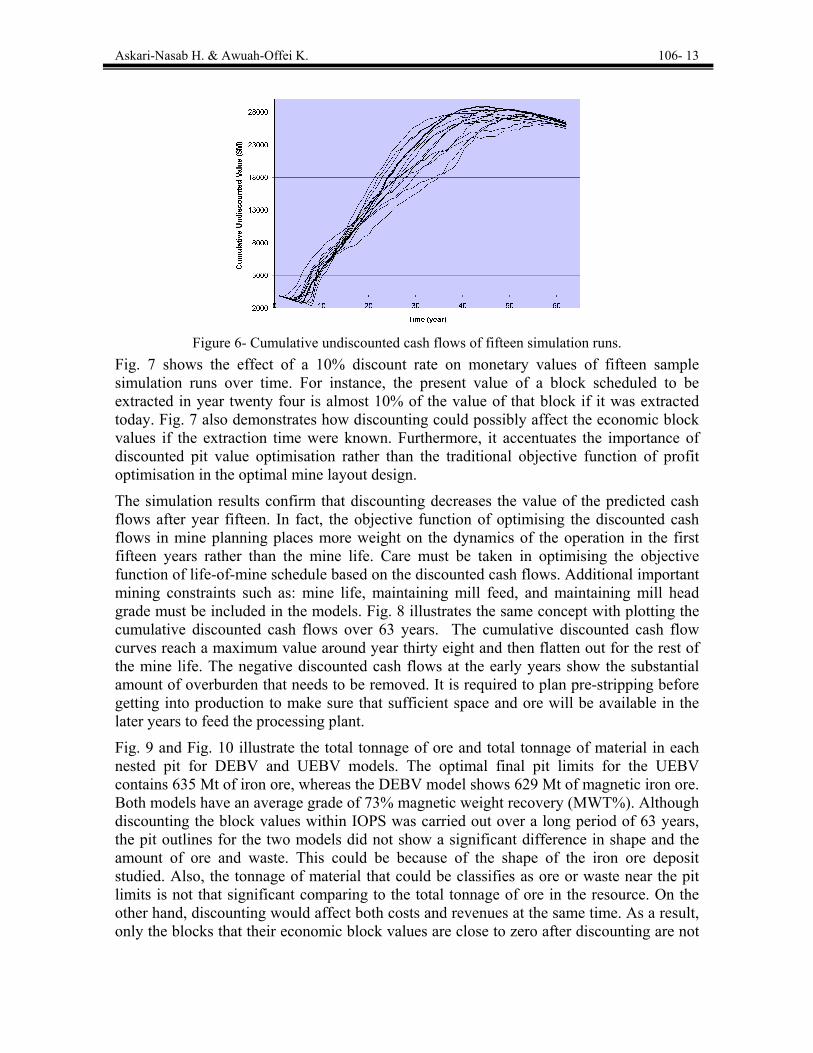
Fig. 6 illustrates the cumulative undiscounted cash flow of fifteen sample push-back simulation iterations out of 3000 iterations over 63 years. A range of feasible mining starting points and different push-back scenarios were simulated by IOPS. The learning agent interacts with the push-back simulation runs to generate the optimal push-back schedule. Given that the final pit limits is not defined at this stage, the simulation generates push-backs with increase in the cumulative cash flows until it reaches a climax where the cost of mining exceeds the generated revenue. Fig. 6 also demonstrates how the cumulative cash flows start declining when the pushback simulation passes the possible final pit limits.


Figure 6- Cumulative undiscounted cash flows of fifteen simulation runs.

Fig. 7 shows the effect of a 10% discount rate on monetary values of fifteen sample simulation runs over time. For instance, the present value of a block scheduled to be extracted in year twenty four is almost 10% of the value of that block if it was extracted today. Fig. 7 also demonstrates how discounting could possibly affect the economic block values if the extraction time were known. Furthermore, it accentuates the importance of discounted pit value optimisation rather than the traditional objective function of profit optimisation in the optimal mine layout design.

The simulation results confirm that discounting decreases the value of the predicted cash flows after year fifteen. In fact, the objective function of optimising the discounted cash flows in mine planning places more weight on the dynamics of the operation in the first fifteen years rather than the mine life. Care must be taken in optimising the objective function of life-of-mine schedule based on the discounted cash flows. Additional important mining constraints such as: mine life, maintaining mill feed, and maintaining mill head grade must be included in the models. Fig. 8 illustrates the same concept with plotting the cumulative discounted cash flows over 63 years. The cumulative discounted cash flow curves reach a maximum value around year thirty eight and then flatten out for the rest of the mine life. The negative discounted cash flows at the early years show the substantial amount of overburden that needs to be removed. It is required to plan pre-stripping before getting into production to make sure that sufficient space and ore will be available in the later years to feed the processing plant.

Fig. 9 and Fig. 10 illustrate the total tonnage of ore and total tonnage of material in each nested pit for DEBV and UEBV models. The optimal final pit limits for the UEBV contains 635 Mt of iron ore, whereas the DEBV model shows 629 Mt of magnetic iron ore. Both models have an average grade of 73% magnetic weight recovery (MWT%). Although discounting the block values within IOPS was carried out over a long period of 63 years, the pit outlines for the two models did not show a significant difference in shape and the amount of ore and waste. This could be because of the shape of the iron ore deposit studied. Also, the tonnage of material that could be classifies as ore or waste near the pit limits is not that significant comparing to the total tonnage of ore in the resource. On the other hand, discounting would affect both costs and revenues at the same time. As a result, only the blocks that their economic block values are close to zero after discounting are not


considered within the pit limits for the discounted model. Fig. 11 demonstrates the anticipated value difference between the undiscounted and discounted pit values.

Figure 7- Discounted annual cash flows of fifteen simulation runs.

Figure 8- Cumulative discounted cash flows of fifteen simulation runs.

Figure 9- Tonnage of ore in the discounted and undiscounted nested pits.


Figure10- Total tonnage of material in the discounted and undiscounted nested pits.

Figure 11- Undiscounted and discounted pit values.

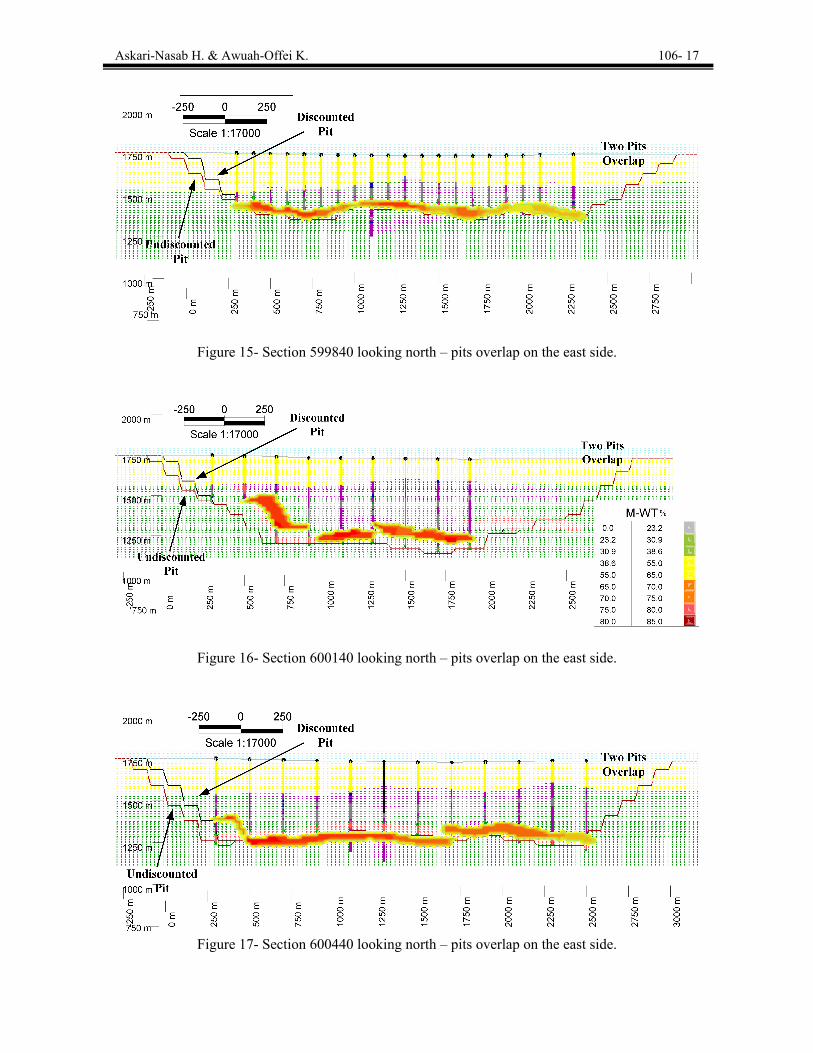
The investigation of the shape of the final pit limits on cross sections in various directions revealed an overlap of two pits in most of the areas. Fig. 12 to 14 illustrate cross sections of the deposit with the final pit outlines based on the UEBV and DEBV models looking west. The legend is representing the iron ore grade based on MWT%. The two final pits lie on top of each other on the northern part of the deposit. On the southern part of the deposit the two pits separate and have more difference in shape as they progress in the eastern direction. Fig. 15 to 17 demonstrate the deposit and the pit outlines looking north. The UEBV and DEBV pits completely overlap on the eastern side and there is a small difference on the western wall.

The differences between the two outlines are due to the fact that the decrease in economic block values because of discounting in certain marginal areas is more than the effect of discounting on the cost of removing some of the overlying waste blocks, which are not within the same extraction period. In fact, the revenue generated by the marginal ore blocks are discounted with a higher rate comparing to the waste blocks positioned at an earlier extraction period. As a result in the LG algorithm the revenue generated by the marginal ore blocks can not cover the costs of removing the waste covering them.


Figure 12- Section 98000 looking west- two pits completely overlap.

Figure 13- Section 98300 looking west- two pits overlap on the northern side.

Figure 14- Section 98500 looking west – the difference gets larger.


Figure 15- Section 599840 looking north – pits overlap on the east side.




The effect of discounting could have an impact on the optimised final outlines of larger deposits with a smaller annual production targets. The shape of the final pit limits would have a direct effect on the reserves and average grades reported. As a matter of fact the impact of the time aspect of extraction would influence how resources and reserves are classified. The results of the case study are an evidence for how using the classical approach could result in overestimation of reserves. Furthermore, the case study validates that the optimal long term schedule is constrained by the conventional ultimate pit layouts. It also, confirms Caccetta and Hill (2003) theorem stated in the introduction.

5. Conclusions

The paper investigated the validity of the theorem presented by Caccetta and Hill (2003) through a case study using the intelligent agent-based mine planning simulator (IOPS)(Askari-Nasab et al., 2005; Askari-Nasab, 2006; Askari-Nasab et al., 2007; Askari-Nasab and Szymanski, 2007; Askari-Nasab et al., 2008). Caccetta and Hill (2003) theorem states that a final pit limits designed directly by using an optimal long-term schedule will result in a pit outline that is a subset of the conventional final pit layouts generated by the Lerchs Grossmann’s (LG) algorithm. The study has been based on the fact that if the optimal schedule is known, then the extraction time of each block would also be known. Given the extraction time, the block values could be discounted. Then, the present value of blocks would be used in determining the pit outline using the LG algorithm. The resultant pit outline using the discounted block values would be based on the maximum present value of the pit rather than the maximum profit. A comparative analysis between the undiscounted and discounted models would then reveal the variation between the two outlines. The intelligent agent-based mine planning simulator, IOPS, was used to determine the optimal push-back schedule prior to determining the final pit outline. The resultant push-back schedule was used to construct a discounted economic block model; this block model was used as input to the LG algorithm.

A case study of an iron ore deposit was completed on a tabular deposit extended in a north-south direction with 139 exploration drillholes. The processing plant was founded on magnetic separators. Consequently, magnetic weight recovery (MWT) of iron ore was used as the main criterion for defining ore. Drillhole compositing was taken place based on similar rock types with three types of ore: top magnetite, oxide, and bottom magnetite. Kriging was used to build the geological block model containing 883,200 blocks that makes a model framework with dimensions of 160X×120Y×46Z blocks. Three thousand iterations of simulation runs using IOPS with a mining capacity of 150

generated a push-back schedule over 63 years. Given that, no final limits were defined the sixty three years is not the mine life and it is representing the time that is required to extract all the blocks within the block model enforcing feasible slope constraints. Afterwards, the block values were discounted with respect to the IOPS optimal schedule. Bench phases technique was used to determine the final pit limits using the LG algorithm for the discounted and undiscounted models.

1−× yeartonnemillion

The optimal final pit limits for the undiscounted model includes 635 Mt of iron ore, where the discounted model showed 629 Mt of magnetic ore. Both models had an average grade of 73% magnetic weight recovery (MWT%). Although discounting the block values within IOPS was carried out over a long period of 63 years, the pit outlines for the two models did


not show a significant difference in shape and the amount of ore and waste. The differences between the two outlines are due to the fact that the decrease in economic block values because of discounting in certain marginal areas is more than the effect of discounting on the cost of removing some of the overlying waste blocks, which are not within the same extraction period. In fact, the revenue generated by the marginal ore blocks are discounted with a higher rate comparing to the waste blocks positioned at an earlier extraction period.

Examination of the shape of the pit on cross sections demonstrated overlap of two pits in most of the areas with deviations in the southern and eastern side of the pit. The analyses and comparisons of the results demonstrate that indeed the optimal long term schedule is constrained by the conventional ultimate pit layouts. Therefore, obtaining the optimal production schedule of a mine by first determining the final pit outline and then generating the schedule is a valid practice. However, this could overstate the reserves of larger deposits with a smaller annual production targets and might lead to over-capacity design.

The intelligent agent framework used in this study provides a powerful basis for addressing the real size open pit mine planning problems. Further focused research is underway to develop and test the models based on intelligent agents to include more critical mine planning variables such as: optimised cut-off grades, mill feed requirements, blending parameters, and stockpile constraints into the intelligent mine planning framework. Stochastic simulation as one of the major entities of the developed models has the ability to address the random field and stochastic variables involved in mine planning. The intelligent agent framework has the capability to be extended for the optimal integration of mining and mineral processing systems, and development of a framework to quantify uncertainty relevant to mine planning and engineering design.

6. References

[1] Askari-Nasab, H., (2006), "Intelligent 3D interactive open pit mine planning and optimization", PhD Thesis Thesis, © University of Alberta, Edmonton, Canada, Pages 167.

[2] Askari-Nasab, H., Awuah-Offei, K., and Frimpong, S., (2004), "Stochastic simulation of open pit pushbacks with a production simulator", in Proceedings of CIM Mining Industry Conference and Exhibition, © Edmonton, Alberta, Canada, pp. on CD-ROM.

[3] Askari-Nasab, H., Frimpong, S., and Awuah-Offei, K., (2005), "Intelligent optimal production scheduling estimator", in Proceedings of 32nd Application of Computers and Operation Research in the Mineral Industry, © Taylor & Francis Group, London, Tucson, Arizona, USA, pp. 279-285.

[4] Askari-Nasab, H., Frimpong, S., and Szymanksi, J., (2007), "Modeling open pit dynamics using discrete simulation", International Journal of Mining, Reclamation and Environment, Vol. 21, 1, pp. 35- 49.


[5] Askari-Nasab, H., Frimpong, S., and Szymanksi, J., (2008), "Investigating the continuous time open pit dynamics", The Journal of the South African Institute of Mining and Metallurgy, Vol. 108, 2, pp. 61-73.

[6] Askari-Nasab, H. and Szymanski, J., (2007), "Open pit production scheduling using reinforcement learning", in Proceedings of 33rd International Symposium on Computer Application in the Minerals Industry (APCOM), © GECAMIN LTDA, Santiago, Chile, pp. 321-326.

[7] Caccetta, L. and Hill, S. P., (2003), "An application of branch and cut to open pit mine scheduling", Journal of Global Optimization, Vol. 27, November, pp. 349 - 365.

[8] Caccetta, L. and Hill, S. P., (2003), "An application of branch and cut to open pit mine scheduling", Journal of Global Optimization, Vol. 27, November, pp. 349-365.

[9] Dagdelen, K. and Kawahata, K., (2007), "Oppurtunities in Multi-Mine Planning through Large Scale Mixed Integer Linear Programming Optimization", in Proceedings of 33rd International Symposium on Computer Application in the Minerals Industry (APCOM), © GECAMIN LTDA, Santiago, Chile, pp. 337-342.

[10] Denby, B., Schofield, D., and Hunter, G., (1996), "Genetic algorithms for open pit scheduling - extension into 3-dimensions", in Proceedings of 5th International Symposium on Mine Planning and Equipment Selection, © A.A.Balkema/Rotterdam/Brookfield, Sao Paulo, Brazil, pp. 177-186.

[11] Deutsch, C. V., (2002), "Geostatistical reservoir modeling", © Oxford University Press, New York, Pages 162 - 166.

[12] Dogbe, G. and Frimpong, S., (2004), "Integrated open pit optimization with periodic material scheduling", in Proceedings of CIM Mining Industry Conference and Exhibition, © Edmonton, pp. CD ROM.

[13] Elveli, B., (1995), " Open pit mine design and extraction sequencing by use OR and AI concepts", International Journal of Surface Mining, Reclamation and Environment, Vol. 9, pp. 149-153.

[14] Erarslan, K. and Celebi, N., (2001), "A simulative model for optimum open pit design", The Canadian Mining and Metallurgical Bulletin, Vol. 94, October, pp. 59-68.

[15] Gemcom Software International, I., (1998-2007), "Whittle strategic mine planning software", ver. 4.00, Vancouver, B.C.: Gemcom Software International.

[16] Johnson, T. B. and Barnes, R. J., (1988), "Application of the maximal flow algorithm to ultimate pit design", in Engineering design : better results through


operations research methods, Vol. 8, Publications in operations research series, R. R. Levary, Ed. New York, © North-Holland, pp. xv, 713.

[17] Lerchs, H. and Grossmann, I. F., (1965), "Optimum design of open-pit mines", The Canadian Mining and Metallurgical Bulletin, Transactions, Vol. LXVIII, pp. 17-24.

[18] Murariu, V. and Svoboda, J., (2003), "The applicability of Davis tube tests to ore separation by drum magnetic separators", Physical Separation in Science and Engineering, Vol. 12, 1, pp. 1-11.

[19] Ramazan, S., Dagdelen, K., and Johnson, T. B., (2005), "Fundamental tree algorithm in optimising production scheduling for open pit mine design", Mining Technology : IMM Transactions section A, Vol. 114, 1, pp. 45-54.

[20] Ramazan, S. and Dimitrakopoulos, R., (2004), "Traditional and new MIP models for production scheduling with in-situ grade variability", International Journal of Surface Mining, Reclamation & Environment, Vol. 18, 2, pp. 85-98.

[21] Sutton, R. S. and Barto, A. G., (1998), "Reinforcement Learning, An Introduction", © The MIT Press, Cambridge, Massachusetts, Pages 432.

[22] Tolwinski, B. and Underwood, R., (1992), "An algorithm to estimate the optimal evolution of an open pit mine", in Proceedings of 23rd APCOM Symposium, © SME, Littleton, Colorado, University of Arizona, pp. 399 - 409.

[23] Whittle, J., (1989), "The facts and fallacies of open-pit design," in Manuscript, Whittle Programming Pty Ltd. North Balwyn, Victoria, Australia

[24] Wooldridge, M., (2002), "An Introduction to Multi-Agent Systems", © John Wiley and Sons Limited, Chichester, UK, Pages 348.

[25] Yegulalp, T. M. and Arias, J. A., (1992), "A fast algorithm to solve the ultimate pit limit problem", in Proceedings of 23rd APCOM Symposium, © AIME, Littleton, Colorado, pp. 391-397.

[26] Zhao, Y. and Kim, Y. C., (1992), "A new optimum pit limit design algorithm", in Proceedings of 23rd APCOM Symposium, © SME, Littleton, Colorado, University of Arizona, pp. 423-434.

askari-nasab h. & awuah-offei k. 106- 1 106 open pit

Documents