assessing drought cycles in spi time series using a ... · correspondence to: e. moreira...

Nat. Hazards Earth Syst. Sci., 15, 571–585, 2015

www.nat-hazards-earth-syst-sci.net/15/571/2015/

doi:10.5194/nhess-15-571-2015

© Author(s) 2015. CC Attribution 3.0 License.

Assessing drought cycles in SPI time series using a Fourier analysis

E. E. Moreira1, D. S. Martins2, and L. S. Pereira3

1CMA – Center of Mathematics and Applications, Faculty of Sciences and Technology, Nova University of Lisbon,

2829-516 Caparica, Portugal2Institute Dom Luiz, Faculty of Sciences, University of Lisbon, 1749-016 Lisbon, Portugal3LEAF, Research Center for Landscape, Environment, Agriculture and Food, Institute of Agronomy, University of Lisbon,

1349-017 Lisbon, Portugal

Correspondence to: E. Moreira ([email protected])

Received: 28 February 2014 – Published in Nat. Hazards Earth Syst. Sci. Discuss.: 23 April 2014

Revised: 23 February 2015 – Accepted: 24 February 2015 – Published: 13 March 2015

Abstract. In this study, drought in Portugal was assessed us-

ing 74 time series of Standardized Precipitation Index (SPI)

with a 12-month timescale and 66 years length. A cluster-

ing analysis on the SPI Principal Components loadings was

performed in order to find regions where SPI drought char-

acteristics are similar. A Fourier analysis was then applied to

the SPI time series considering one SPI value per year rela-

tive to every month. The analysis focused on the December

SPI time series grouped in each of the three identified clus-

ters to investigate the existence of cycles that could be related

to the return periods of droughts. The most frequent signif-

icant cycles in each of the three clusters were identified and

analysed for December and the other months. Results for De-

cember show that drought periodicities vary among the three

clusters, pointing to a 6-year cycle across the country and a

9.4-year cycle in central and southern Portugal. Both these

cycles likely show the influence of the North Atlantic Os-

cillation (NAO) on the occurrence and severity of droughts

in Portugal. Relative to other months it was observed that

cycles varied according to the common occurrence of pre-

cipitation: for the rainy months – November, December and

January – cycles are similar to those for December; for the

dry months – May to September – where the lack of precipi-

tation masks the occurrence of drought, the dominant cycles

are of short duration and cannot be related to the NAO or

other large circulation indices to explain drought variability;

for the transition months – February, March, April and Octo-

ber – 6-year and 3-year cycles were identified, the latter be-

ing more strongly apparent in central and southern Portugal.

NAO influence is again identified relative to the 6-year cy-

cles. The short cycles are apparently associated with positive

SPI, thus with wetness, not drought. Overall, results confirm

the importance of the NAO as a driving force for dry and wet

periods.

1 Introduction

The cyclicity of climatic and Earth surface processes such as

precipitation, streamflow and droughts is the object of a vari-

ety of studies aimed at better understanding their variability

and identifying possible driving forces. With this objective,

some studies aimed at the reconstruction of past climate se-

ries to allow a better analysis of past and present droughts.

This was the case for a study used to reconstruct drought

time series with historical data (1502–1899) relative to the

south-eastern Mexico, that led to the discovery of cycles of

several periodicities likely related to the El Niño–Southern

Oscillation (ENSO) and solar activity (Mendoza et al., 2006).

Another example is a study using historical data from Sicily,

from 1565 to 1915, that also identified several periodicities

of droughts, particularly related to solar cycles (Piervitali and

Colacino, 2001).

Studies referring to recent time series of precipitation,

streamflow and drought indices are of particular interest for

understanding the influences of large scale indices of atmo-

spheric circulation on drought occurrence and severity. To

assess the cyclicity of drought occurrence, various methods

can be used and applied to those time series, such as various

approaches to the Fourier analysis (Rodrigo et al., 2000; Ya-

dava and Ramesh, 2007), also called spectral analysis (Bordi

et al., 2004a, b; Mitra et al., 1991; Telesca et al., 2013),

Published by Copernicus Publications on behalf of the European Geosciences Union.

572 E. Moreira et al.: Assessing drought cycles in SPI time series using Fourier analysis

and the wavelet transform analysis (Labat, 2006; Prokoph et

al., 2012; Li et al., 2013). Fourier analysis uses the Fourier

decomposition of series and the periodogram device (Pol-

lock, 1999; Bloomfield, 2000) with the aim of finding cycles

within a given time series.

Research generally aims at finding a better explanation of

time and space variability of the processes and relating the

detected cycles with the periodicity of sea-surface anomalies,

solar cycles or large-scale indices of atmospheric circulation.

Studies with annual or monsoon precipitation data series of-

ten identified cycles of around 11 years which were related to

solar activity cycles (Mazzarella and Palumbo, 1992; Mitra

et al., 1991; Yadara and Ramesh, 2007; Chattopadhyay and

Chattopadhyay, 2011). Studies on solar cycles were reported

by Tsiropoula (2003) and Hathaway (2010). The cycle of so-

lar activity is characterized by the rise and fall in the number

and surface area of sunspots ranging between 9 and 13 years

and averaging 11 years (Hathaway, 2010).

Streamflow periodicities could also be related to solar cy-

cles (e.g. Prokoph et al., 2012). A streamflow study rela-

tive to Europe (Labat, 2006) has shown interannual 4- to

5-year, 14-year and multidecadal 25- and 50-year oscilla-

tions. Gómiz-Fortis et al. (2011) studied streamflow vari-

ability in the Ebro basin and found that respective oscilla-

tion have different periodicity among the sub-regions con-

sidered. Rodríguez-Puebla et al. (1999) used 50-year series

of 3-month cumulated precipitation in the Iberian Peninsula

and applied principal component analysis (PCA). They de-

tected that the North Atlantic Oscillation (NAO) was the ma-

jor source of interannual variability in winter precipitation

and observed that the time series of precipitation and the

NAO had a common peak at about 8 years while showing a

significant coherence. An analysis of rainfall variability rel-

ative to southern Spain found an alternation of wet and dry

periods, with various periodicities, that allowed authors to

identify the NAO among the most possible causal mecha-

nisms in the region (Rodrigo et al., 2000). The precipitation

variability study by Lucero and Rodríguez (2002) stated that

“the first principal component of the transformed bidecadal

component of annual rainfall anomalies attains its positive

(negative) peak about 3 years before the bidecadal compo-

nent of NAO reaches its negative (positive) peak”.

Bordi et al. (2004a) using PCA applied to SPI with 24-

month timescale (SPI-24) for the Elba basin and Sicily found

significant peaks for periodicities of 9.6 years for Sicily and

12.0–9.6 years for Elbe basin. However, significant relations

with the NAO or the ENSO were not found. In addition, other

relevant peaks were close to the 11-year solar cycle. Telesca

et al. (2013) used the SPI with various timescales and ap-

plied a spectral analysis to each local time series in the Ebro

basin, Spain. For both the SPI-12 and 24, authors found cy-

cles of 3.1, 4.1, 5.3, 8.8 and 17.6 years for most locations.

The 3–5-year band was considered to be related to the NAO

(Telesca et al., 2013). Various studies show that cyclicity can

be found for precipitation, streamflow and droughts and that

different methodological approaches lead to coherent results,

with observed cycles relating well with those of the NAO,

the AO and the ENSO, as well as with solar cycles. The

detected cyclicity varies among sub-regions identified with

PCA and cluster analysis. That cyclicity is both observed

for Europe and elsewhere. The precipitation study by Liang

et al. (2011) applied to Northwest China identified signifi-

cant periods of 2.3 and 3.3 years, i.e. not very different from

results by Bordi et al. (2004b) that characterized droughts

with SPI-24 and studied their variability with PCA in east-

ern China. The application of a spectral analysis to a prin-

cipal component led to the detection of peaks characterizing

the interdecadal, decadal and interannual variability. A broad

band peak was found for the interannual timescale of 3.7–

4.0 years; other peaks lie near 6.9–8 up to 16 years and larger.

Results by Liu et al. (2013) using the PDSI, also detected

cycles of 3–5, 5–7 and 8–10 years throughout the Qinghai

Province. Li et al. (2013) used clustering to define drought

sub-regions in Southwest China with SPI and observed dis-

tinctive temporal evolution patterns of droughts in each sub-

region. The cycles varied from 2–3 years to 5–7 years.

The results of a previous study with log-linear models ap-

plied to droughts in southern Portugal showed the existence

of a long-term periodicity that could reflect the natural vari-

ability of the climate (Moreira et al., 2006). This long-term

periodicity was expressed by the alternation between long

periods with high and low frequencies of severe and extreme

droughts. A recent study using ANOVA-like inference cou-

pled with log-linear models applied to 10 long series across

Portugal also suggested a cyclic behaviour of droughts with

periodicity ranging from 26 to 30 years, mostly for the sites

in central and southern Portugal (Moreira et al., 2012). These

studies suggested using Fourier analysis to detect the various

cycles that contribute to the variability of droughts. More-

over, since cyclicity varies from one region to another (Bordi

et al., 2004a, b, 2006; Raziei et al., 2009; Santos et al., 2010;

Telesca et al., 2013), the use of PCA and cluster analysis has

been considered for identifying possible regions within the

country.

Recently, Martins at al. (2012) used PCA applied to the

SPI-12 to identify the main spatial and temporal patterns of

precipitation and drought in Portugal. This approach could

then be combined with the Fourier analysis to verify if the

cycles would change with the considered region.

Considering the review presented, the objective of this

study is to detect the cyclicity of droughts defined through

the SPI-12 and to observe when that cyclicity varies among

identified regions within the country. On one hand, the anal-

ysis focused on the month of December, in the middle of the

rainy season, and the cyclicity of negative peaks of the SPI-

12, which indicate the possible cyclicity of droughts and any

possible influence on drought occurrence of large-scale in-

dices of atmospheric circulation. On the other hand, it was

also aimed at analysing the cyclicity of the SPI-12 for the

other months in the year, i.e. the dry and transition months.

Nat. Hazards Earth Syst. Sci., 15, 571–585, 2015 www.nat-hazards-earth-syst-sci.net/15/571/2015/

E. Moreira et al.: Assessing drought cycles in SPI time series using Fourier analysis 573

In contrast to Santos et al. (2010) and Telesca at al. (2013),

the adopted approach applies Fourier analysis individually

to each SPI-12 time series and an analysis of frequency on

the significant cycles found inside each sub-region was per-

formed in the following. Furthermore, a correspondence is

sought between the minima of the sinusoidal functions and

the moderate, severe and extreme drought events.

2 Data, SPI, clustering and Fourier analysis

2.1 Base information

The data consists of monthly precipitation time series from

1941 to 2006 (66 years) of 74 sites across Portugal (Fig. 1).

Data from weather stations were obtained from the meteo-

rological services (IPMA) and those of rainfall stations re-

fer to the environmental services (SNHIR). Data quality was

assessed using the Kendall autocorrelation test, the Mann–

Kendall trend test and the homogeneity tests of Mann Whit-

ney for the mean and the variance (Helsel and Hirsch, 1992).

To estimate missing values of monthly precipitation, mainte-

nance of variance extension techniques were applied (Hirsch,

1982; Vogel and Stedinger, 1985). These data sets, previously

used in other studies (e.g. Paulo et al., 2012; Martins et al.,

2012; Raziei et al., 2014) were completed with techniques

described by Rosa et al. (2010). Series retained did not have

more than 250 gaps and all series covered the referred period

of 66 years.

Precipitation based drought indices are the first indicators

of droughts, since hydrological droughts may emerge sev-

eral months after a meteorological drought has been initiated

(Wilhite and Buchanan-Smith, 2005). The Standardized Pre-

cipitation Index, SPI (McKee et al., 1993, 1995), which is

often used for identification of drought events and to eval-

uate their severity through well-defined drought classes, is

adopted in this study following results obtained in previ-

ous studies characterizing droughts in Portugal (Paulo and

Pereira, 2006; Santos et al., 2010; Martins et al., 2012).

The SPI is widely used because it is standardized and

therefore allows a reliable comparison between different lo-

cations and climates (Mishra and Singh, 2010). It may be

computed on shorter or longer timescales, which reflect dif-

ferent lags in the response of the water cycle to precipitation

anomalies (Steinemann et al., 2005). In addition, due to its

standardization, its range of variation is independent of the

aggregation timescale of reference, as well as the particu-

lar location and climate. The 12-month timescale, as well as

larger timescales, identifies anomalous dry and wet periods

of relatively long duration and relates well with the impacts

of drought on the hydrologic regimes and water resources of

a region (Vicente-Serrano, 2006), or to the effects of fluctua-

tion in rainfall over short intervals (Mishra and Singh, 2010).

Shorter timescales of less than 6 months are more useful

for detecting agricultural droughts and while longer ones,

Figure 1. Spatial distribution of the meteorological stations (×) and

rainfall stations (N) used in the study and delimitation of drought

clusters; (* station included in cluster 3).

i.e. larger than 24 months, may be useful for considering im-

pacts on groundwater resources. For the Portuguese condi-

tions, where a dry summer period of nearly 6 months occurs,

droughts impacting the hydrologic regime are better assessed

using the 12-month timescale (Paulo and Pereira, 2006; San-

tos et al., 2010). Hence, previous studies on drought variabil-

ity and drought class transitions were performed with the SPI

12-month (Moreira et al., 2006, 2012; Martins et al., 2012).

Therefore, time series of SPI with a 12-month timescale

(SPI-12) were computed from the 74 monthly precipitation

time series. The respective monthly drought classes were

then computed based on Table 1.

The computation of the SPI index (Guttman, 1999) in a

given year i and calendar month j , for a k timescale was

performed with the following steps: (i) calculation of a cu-

mulative precipitation series

Xk(i,j), i = 1, . . .,n;j = 1, . . .,12,k = 1,2, . . .,12, . . .

for that calendar month j , where each term is the sum of

the actual monthly precipitation with the precipitation of the

k-1 past consecutive months; (ii) fitting of a gamma distri-

www.nat-hazards-earth-syst-sci.net/15/571/2015/ Nat. Hazards Earth Syst. Sci., 15, 571–585, 2015


Table 1. SPI drought class classification (McKee et al., 1993).

Drought Time in

Code classes SPI values category (%)

1 Non-drought SPI≥ 0

2 Near normal −1<SPI< 0 34.1

3 Moderate −1.5<SPI≤−1 9.2

4 Severe −2<SPI≤−1.5 4.4

5 Extreme SPI≤−2 2.3

bution function F(x) to the monthly series; (iii) computing

the non-exceedance probabilities corresponding to the cumu-

lative precipitation values; (iv) transforming those probabili-

ties into the values of a standard normal variable, which are

actually the SPI values. For example, when k = 12 months,

the SPI in December includes the effect of precipitation in

December and in the previous 11 months. For the climate of

Portugal, SPI-12 values of December are considered a good

reference for drought monitoring because this month is cen-

tral in the rainy season; thus, when droughts occur the effect

of lack of precipitation in the previous months is then well

detected. In contrast, selecting a summer month, for instance

July, which falls in the dry season where precipitation is al-

most non-existent, the dryness identified may not be signif-

icant for drought monitoring despite the fact that the SPI-12

in July considers the effect of all precedent 11 months. In this

study, the main focus of the Fourier analysis was on the SPI-

12 for December, where the significant cycles retained for

continental Portugal are discussed (Sect. 3.2). Additionally,

a discussion of the drought cycles found using the SPI-12

for the remaining months, January–November, is provided in

Sect. 3.3.

In order to identify regions with the same spatial and tem-

poral patterns of droughts, a PCA on the SPI-12 was per-

formed and followed by a K-means clustering of the PC load-

ings provided by the PCA. The adoption of PCA followed by

a cluster analysis is justified by the need to take into consid-

eration the spatial variability of the periodicity that droughts

may assume. The PCA is a method commonly used in studies

of climate and is often applied to drought indices and precip-

itation to identify their patterns (Bordi et al., 2004a, b, 2006;

Raziei et al., 2009; Santos et al., 2010). This method allows

reduction of the original dimensionality of the data through

forming new uncorrelated variables that are linear combina-

tions of the original ones and explain a large portion of the

total variance (Sharma, 1996). Here, the PCA was applied in

the S-mode (Richman, 1986), using the 74 SPI-12 time se-

ries in order to capture the drought variability which shows

the co-variability between stations considering its time vari-

ability (Martins et al., 2012). Furthermore, to identify regions

with different drought variability, the varimax rotation was

used (Raziei et al., 2009).

The loadings obtained from the PCA, which represent the

correlation between the original data and the principal com-

ponents series, were then submitted to a cluster analysis. This

classification method is used to detect variables that are more

similar to each other and categorize them together in different

clusters (Sharma, 1996). From the various types of methods,

the K-means clustering was used herein since it is suitable

for climate data and also facilitates comparison of the results

with previous studies that used the same method (Santos et

al., 2010).

2.2 Fourier analysis of SPI-12 time series

Regular or near-regular cycles are often encountered in na-

ture. The Fourier analysis methodology can be referred to as

a method for uncovering hidden periodicities and, in particu-

lar, extracting regular cyclical components from the time se-

ries when the quantity of data is not excessively large. Fourier

analysis is a method based upon the Fourier decomposition

of a series, which is a matter of explaining the series entirely

as a composition of sinusoidal functions. This originates in

the idea that, over a finite interval, any analytic function can

be approximated, to whatever degree of accuracy is desired,

by taking a weighted sum of sine and cosine functions (Pol-

lock, 1999).

Letm= n/2 if n is even orm= (n−1)/2 if n is odd, with

n the number of observations in a time series. The general

model for a cyclic fluctuation would include the frequencies,

ωj = (2πj)/n, j = 0, . . .,m which are equally spaced in the

interval [0, π ] and take the form

yt =

m∑j=0

{αj,1 sin

(ωj t

)+αj,2 cos

(ωj t

) }+ et ,

where t represents time, αj,1 and αj,2, j = 0, . . .,m are es-

timable parameters and et , t = 1, . . .,n are independent and

identically distributed random variables with null mean value

and variance σ 2, representing the residual element which is

called the white noise process (Pollock, 1999).

The factor θj =√α2j,1+α

2j,2, j = 0, . . .,m, is the ampli-

tude of the j th periodic component and indicates the impor-

tance of that component within the sum. The parameters αj,1and αj,2, j = 0, . . .,m are estimated using the least squares

method and the expressions for their estimators are given by

(Pollock, 1999)

α̃0,2 =

∑nt=1yt

n; α̃j,1 =

2∑nt=1sin(ωj t)yt

n;

α̃j,2 =2∑nt=1cos(ωj t)yt

n,j = 1, . . .,m.

Then an estimator for θj , θ̃j , can be obtained and a statistic

to test the significance of the j th periodic component is given

by (Fisher, 1929; Nowroozi, 1967)

gj =θ̃2j∑m

i=1θ̃2i

,j = 1, . . .,m.



The total sample variance is given by∑mj=1

θ̃2j

2and the pro-

portion of that variance which is attributable to the periodical

component at frequency ωj isθ̃2j

2.

In order to provide a graphical representation of the sam-

ple variance decomposition, the elements of the total vari-

ance must be scaled by a factor of n. The graph of the func-

tion Ij =nθ̃2j

2is known as the classical periodogram (Pol-

lock, 1999). The graphic representation of Ij for j = 1, . . .,m

(Fig. 2), allows one to detect the existence of relevant peri-

odic components of the time series, as well as the importance

of each one. The wavelength, i.e. the period in time units of

the j-th periodic component, is given by pj = n/j .

In the current study, the number of observations is n= 66

in all locations, thusm= 33. For each of the studied time se-

ries, the Ij for j = 1, . . .,m was calculated and graphically

represented in order to visualize the highest peaks, which

correspond to the leading periodic components of the time

series. The observation of several high peaks indicates the

existence of several periodic components with different pe-

riods. However, in general, few of those peaks represent a

strong periodical signal that cannot be assigned to statistical

fluctuations in a merely white noise process.

The assessment of the statistical significance of a peak

involves testing the null hypothesis, H0, that the observed

time series are purely white noise against the alternative,H1,

stating that a periodic signal is present there. The statistical

distribution of the periodogram is well known for the even-

sampling case, which corresponds to equally spaced obser-

vations (Scargle, 1982). The most important result is that if

the observations in the time series are pure Gaussian noise

the Ij ,j = 1, . . .,m are independent and exponentially dis-

tributed. In this situation, it is reliable to use the false alarm

probability to assess the statistical significance of the highest

peaks in the periodogram, which states that if Z=max (Ij ),

j = 1, . . .,m is a maximum value of the periodogram, then

the probability for Z being over the set of the m periodogram

values is given by

Pr(Z > z)= 1− [1− exp(−z)]m.

So, a threshold z0 can be used for detecting if a peak is sig-

nificant, which is defined as

z0 =−ln[1− (1−p0)(1/m)],

where p0 is the false alarm probability, a fixed small value

usually selected between 0.01 and 0.1 (Scargle, 1982). For

instance, in the “Reguengos” December SPI-12 time series

(Fig. 2) the highest peak is attained for j = 11(I11 = 9.05),

which corresponds to a periodic component with a 6-year

period. Choosing a false alarm probability of 0.1, with the

number of periodical components m= 33, the value z0 ob-

tained is 5.75, which allows one to conclude that the peak

is significant. In this time series, two other peaks are signif-

icant, those for j = 2 and j = 7 corresponding to sinusoidal

0

1

2

3

4

5

6

7

8

9

10

0 2 4 6 8 10 12 14 16 18 20 22 24 26 28 30 32

j=2;pj=33 j=7;pj=9.4

j=11;pj=6

a)

-3

-2

-1

0

1

2

3

19

40

19

42

19

44

19

46

19

48

19

50

19

52

19

54

19

56

19

58

19

60

19

62

19

64

19

66

19

68

19

70

19

72

19

74

19

76

19

78

19

80

19

82

19

84

19

86

19

88

19

90

19

92

19

94

19

96

19

98

20

00

20

02

20

04

SPI

R²=33%

R²=14%

b)

Figure 2. Reguengos: (a) graph of Ij , j = 1, . . .,33; (b) SPI De-

cember values (grey dots) vs. fitted sinusoidal wave of 6-year period

(dashed line) vs. fitted model resulting from summing up the waves

with period 6, 9.4 and 33 years (black line).

waves with 33- and 9.4-year periods (Fig. 2). If one consid-

ers a false alarm probability of 0.01 instead of 0.1, then only

the peak for j = 11 with a 6-year period can be considered

significant.

The fitted sinusoidal function of 6-year period is presented

in Fig. 2 simultaneously with the Reguengos time series and

obviously has the best goodness of fit to the time series

among all other periodic components, R2= 0.14 (dashed

line). For a better goodness of fit between the sinusoidal

wave and the time series, the cycles corresponding to the

significant peaks in the periodogram can be summed up,

thus j = 2+ 7+ 11, to build a general model for a non-

regular cyclic fluctuation. In Fig. 2, the wave resulting from

summing up the significant cycles with periods 6, 9.4 and

33 years (black line) is also represented. Some improvement

of the goodness of fit is then obtained, with R2= 0.33.



1

2

3

4

5

1941

1942

1944

1945

1946

1948

1949

1951

1952

1953

1955

1956

1958

1959

1961

1962

1963

1965

1966

1968

1969

1970

1972

1973

1975

1976

1978

1979

1980

1982

1983

1985

1986

1987

1989

1990

1992

1993

1995

1996

1997

1999

2000

2002

2003

2004

Dro

ugh

t cl

asse

s

year

all

1

2

3

4

5

1941

1942

1944

1945

1946

1948

1949

1951

1952

1953

1955

1956

1958

1959

1961

1962

1963

1965

1966

1968

1969

1970

1972

1973

1975

1976

1978

1979

1980

1982

1983

1985

1986

1987

1989

1990

1992

1993

1995

1996

1997

1999

2000

2002

2003

2004

Dro

ugh

t cl

asse

s

year

cluster 1

1

2

3

4

5

194

119

42

194

419

45

194

6

194

819

49

195

1

195

2

195

319

55

195

6

195

8

195

919

6119

62

196

319

65

196

6

196

8

196

919

70

197

2

197

319

75

1976

197

8

197

919

80

198

2

198

3

198

519

86

198

7

198

919

90

199

219

93

199

519

96

1997

199

9

200

020

02

200

3

200

4

Dro

ugh

t cl

asse

s

year

cluster 2

1

2

3

4

5

1941

1942

1944

1945

1946

1948

1949

1951

1952

1953

1955

1956

1958

1959

1961

1962

1963

1965

1966

1968

1969

1970

1972

1973

1975

1976

1978

1979

1980

1982

1983

1985

1986

1987

1989

1990

1992

1993

1995

1996

1997

1999

2000

2002

2003

2004

Dro

ugh

t cl

asse

s

year

cluster 3

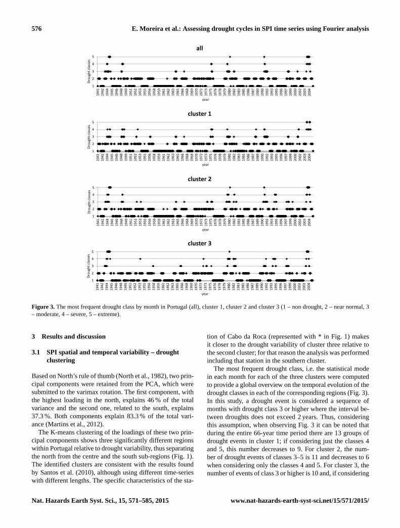
Figure 3. The most frequent drought class by month in Portugal (all), cluster 1, cluster 2 and cluster 3 (1 – non drought, 2 – near normal, 3

– moderate, 4 – severe, 5 – extreme).

3 Results and discussion

3.1 SPI spatial and temporal variability – drought

clustering

Based on North’s rule of thumb (North et al., 1982), two prin-

cipal components were retained from the PCA, which were

submitted to the varimax rotation. The first component, with

the highest loading in the north, explains 46 % of the total

variance and the second one, related to the south, explains

37.3 %. Both components explain 83.3 % of the total vari-

ance (Martins et al., 2012).

The K-means clustering of the loadings of these two prin-

cipal components shows three significantly different regions

within Portugal relative to drought variability, thus separating

the north from the centre and the south sub-regions (Fig. 1).

The identified clusters are consistent with the results found

by Santos et al. (2010), although using different time-series

with different lengths. The specific characteristics of the sta-

tion of Cabo da Roca (represented with * in Fig. 1) makes

it closer to the drought variability of cluster three relative to

the second cluster; for that reason the analysis was performed

including that station in the southern cluster.

The most frequent drought class, i.e. the statistical mode

in each month for each of the three clusters were computed

to provide a global overview on the temporal evolution of the

drought classes in each of the corresponding regions (Fig. 3).

In this study, a drought event is considered a sequence of

months with drought class 3 or higher where the interval be-

tween droughts does not exceed 2 years. Thus, considering

this assumption, when observing Fig. 3 it can be noted that

during the entire 66-year time period there are 13 groups of

drought events in cluster 1; if considering just the classes 4

and 5, this number decreases to 9. For cluster 2, the num-

ber of drought events of classes 3–5 is 11 and decreases to 6

when considering only the classes 4 and 5. For cluster 3, the

number of events of class 3 or higher is 10 and, if considering



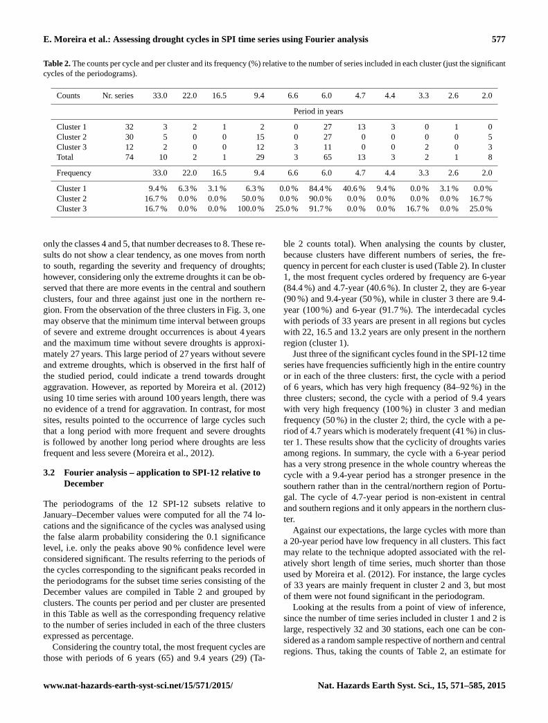
Table 2. The counts per cycle and per cluster and its frequency (%) relative to the number of series included in each cluster (just the significant

cycles of the periodograms).

Counts Nr. series 33.0 22.0 16.5 9.4 6.6 6.0 4.7 4.4 3.3 2.6 2.0

Period in years

Cluster 1 32 3 2 1 2 0 27 13 3 0 1 0

Cluster 2 30 5 0 0 15 0 27 0 0 0 0 5

Cluster 3 12 2 0 0 12 3 11 0 0 2 0 3

Total 74 10 2 1 29 3 65 13 3 2 1 8

Frequency 33.0 22.0 16.5 9.4 6.6 6.0 4.7 4.4 3.3 2.6 2.0

Cluster 1 9.4 % 6.3 % 3.1 % 6.3 % 0.0 % 84.4 % 40.6 % 9.4 % 0.0 % 3.1 % 0.0 %

Cluster 2 16.7 % 0.0 % 0.0 % 50.0 % 0.0 % 90.0 % 0.0 % 0.0 % 0.0 % 0.0 % 16.7 %

Cluster 3 16.7 % 0.0 % 0.0 % 100.0 % 25.0 % 91.7 % 0.0 % 0.0 % 16.7 % 0.0 % 25.0 %

only the classes 4 and 5, that number decreases to 8. These re-

sults do not show a clear tendency, as one moves from north

to south, regarding the severity and frequency of droughts;

however, considering only the extreme droughts it can be ob-

served that there are more events in the central and southern

clusters, four and three against just one in the northern re-

gion. From the observation of the three clusters in Fig. 3, one

may observe that the minimum time interval between groups

of severe and extreme drought occurrences is about 4 years

and the maximum time without severe droughts is approxi-

mately 27 years. This large period of 27 years without severe

and extreme droughts, which is observed in the first half of

the studied period, could indicate a trend towards drought

aggravation. However, as reported by Moreira et al. (2012)

using 10 time series with around 100 years length, there was

no evidence of a trend for aggravation. In contrast, for most

sites, results pointed to the occurrence of large cycles such

that a long period with more frequent and severe droughts

is followed by another long period where droughts are less

frequent and less severe (Moreira et al., 2012).

3.2 Fourier analysis – application to SPI-12 relative to

December

The periodograms of the 12 SPI-12 subsets relative to

January–December values were computed for all the 74 lo-

cations and the significance of the cycles was analysed using

the false alarm probability considering the 0.1 significance

level, i.e. only the peaks above 90 % confidence level were

considered significant. The results referring to the periods of

the cycles corresponding to the significant peaks recorded in

the periodograms for the subset time series consisting of the

December values are compiled in Table 2 and grouped by

clusters. The counts per period and per cluster are presented

in this Table as well as the corresponding frequency relative

to the number of series included in each of the three clusters

expressed as percentage.

Considering the country total, the most frequent cycles are

those with periods of 6 years (65) and 9.4 years (29) (Ta-

ble 2 counts total). When analysing the counts by cluster,

because clusters have different numbers of series, the fre-

quency in percent for each cluster is used (Table 2). In cluster

1, the most frequent cycles ordered by frequency are 6-year

(84.4 %) and 4.7-year (40.6 %). In cluster 2, they are 6-year

(90 %) and 9.4-year (50 %), while in cluster 3 there are 9.4-

year (100 %) and 6-year (91.7 %). The interdecadal cycles

with periods of 33 years are present in all regions but cycles

with 22, 16.5 and 13.2 years are only present in the northern

region (cluster 1).

Just three of the significant cycles found in the SPI-12 time

series have frequencies sufficiently high in the entire country

or in each of the three clusters: first, the cycle with a period

of 6 years, which has very high frequency (84–92 %) in the

three clusters; second, the cycle with a period of 9.4 years

with very high frequency (100 %) in cluster 3 and median

frequency (50 %) in the cluster 2; third, the cycle with a pe-

riod of 4.7 years which is moderately frequent (41 %) in clus-

ter 1. These results show that the cyclicity of droughts varies

among regions. In summary, the cycle with a 6-year period

has a very strong presence in the whole country whereas the

cycle with a 9.4-year period has a stronger presence in the

southern rather than in the central/northern region of Portu-

gal. The cycle of 4.7-year period is non-existent in central

and southern regions and it only appears in the northern clus-

ter.

Against our expectations, the large cycles with more than

a 20-year period have low frequency in all clusters. This fact

may relate to the technique adopted associated with the rel-

atively short length of time series, much shorter than those

used by Moreira et al. (2012). For instance, the large cycles

of 33 years are mainly frequent in cluster 2 and 3, but most

of them were not found significant in the periodogram.

Looking at the results from a point of view of inference,

since the number of time series included in cluster 1 and 2 is

large, respectively 32 and 30 stations, each one can be con-

sidered as a random sample respective of northern and central

regions. Thus, taking the counts of Table 2, an estimate for



the probability that the return period of droughts is 6 years

in cluster 1 is given by 27/32= 84.4 %. In cluster 2 that es-

timate is 27/30= 90 %. Relative to cluster 3, the probability

estimates of 91.7 and 100 % respectively of the return period

of droughts being 6 and 9.4 years is likely overestimated be-

cause the number of time series in the sample is only 12 and

their spatial distribution is not the best; thus the sample may

not be representative of the population, even taking into ac-

count that cluster 3 is small. However, for the entire country a

reliable estimate for the probability of a 6-year return period

is given by 65/74= 87.8 %.

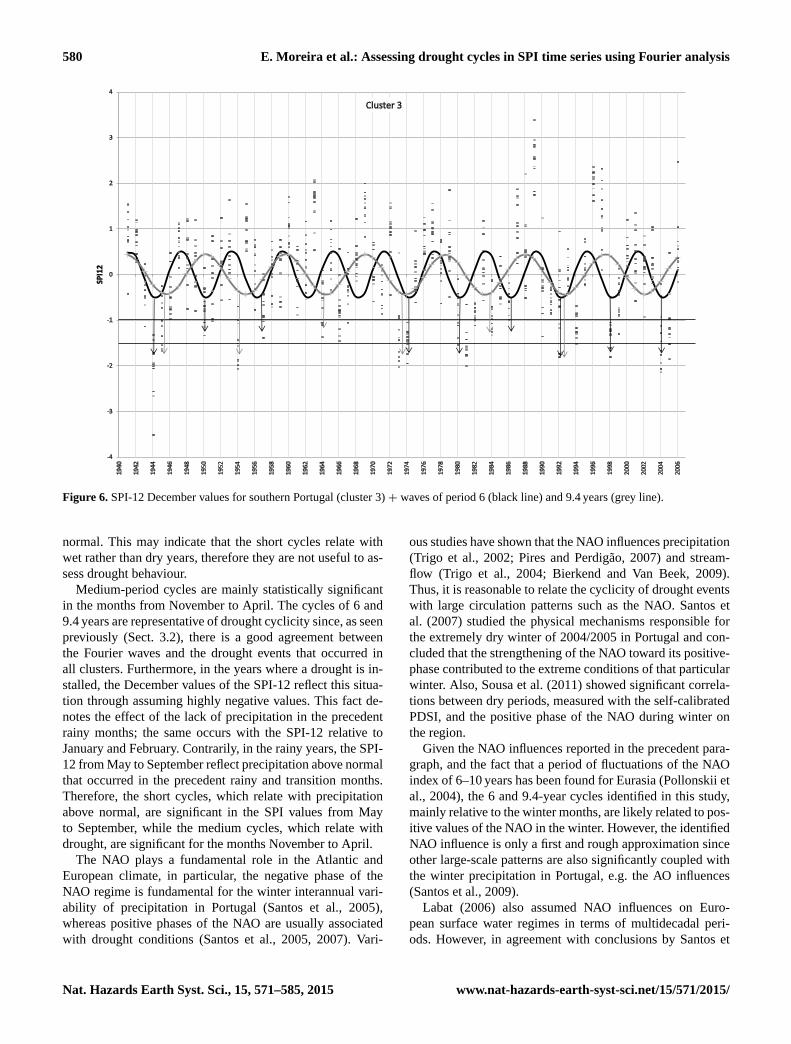
In Figs. 4, 5 and 6, the time series for the SPI-12 relative to

December for the three clusters are shown with superposing

the most frequent waves: one of 4.7-year period in cluster 1,

another of 6-year period in clusters 1, 2 and 3, and a wave

of 9.4-year period in clusters 2 and 3. A correspondence be-

tween the minima of the waves and the SPI upper borders for

moderate drought (−1) and for severe and extreme drought

(−1.5) is established through arrows placed in these figures.

In Fig. 4, relative to cluster 1, one can observe that the wave

of 6-year period has 11 minima and nearly all of them co-

incide with events of moderate (−1.5<SPI<−1) or severe

and extreme droughts (SPI<−1.5). Just one drought event,

in 1957, was missed by the wave. Therefore, a good visual

agreement exists between the minima of the sinusoidal wave

of 6-year period and the events of moderate or more severe

droughts that occurred during the study period. Relative to

the wave of 4.7-year period in cluster 1, from a total of 14

minima about 11 coincide with events of moderate, severe

and extreme drought. The degree of agreement for this wave

is less good than for the one with a 6-year period.

For cluster 2 (Fig. 5) a good agreement between the min-

ima of the 6-year period wave and the events of moderate,

severe and extreme droughts was observed; as for cluster 1,

the same drought event of 1957 was missed by the wave.

As for the wave of 9.4-year period, six out of a total of

seven minima coincide with events of moderate, severe and

extreme droughts. For cluster 3 (Fig. 6), the visual agree-

ment between the wave of 6-year period and the drought

events is not as good as for the previous clusters, with three

of the minima not coinciding with drought events and with

two events of moderate drought and one of severe drought

missed by the wave. Relative to the 9.4-year wave, one out

of the seven minima does not correspond with a drought

event. Furthermore, two moderate and one severe and ex-

treme drought events are missed by the wave. However, this

less good agreement for cluster 3 may be due to the low num-

ber of time series included there. In general, a visual relation

can be established between the Fourier waves and the events

of drought that occurred in each cluster during the study pe-

riod. The correspondence between the sinusoidal waves and

the drought cyclicity is not perfect because cycles in nature

are only near-regular, thus not providing for a full agreement

with regular waves.

3.3 Application of Fourier analysis to SPI-12 time

series relative to the rainy, transition and dry

months

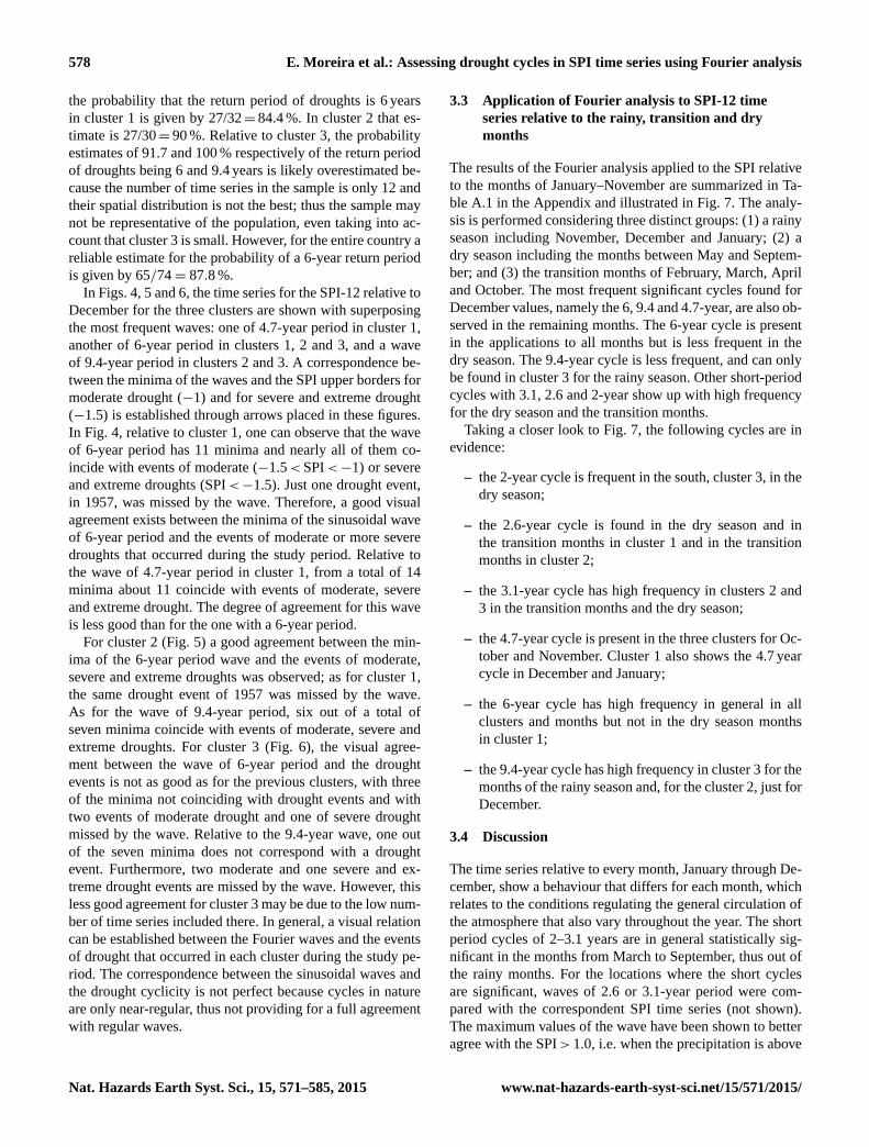
The results of the Fourier analysis applied to the SPI relative

to the months of January–November are summarized in Ta-

ble A.1 in the Appendix and illustrated in Fig. 7. The analy-

sis is performed considering three distinct groups: (1) a rainy

season including November, December and January; (2) a

dry season including the months between May and Septem-

ber; and (3) the transition months of February, March, April

and October. The most frequent significant cycles found for

December values, namely the 6, 9.4 and 4.7-year, are also ob-

served in the remaining months. The 6-year cycle is present

in the applications to all months but is less frequent in the

dry season. The 9.4-year cycle is less frequent, and can only

be found in cluster 3 for the rainy season. Other short-period

cycles with 3.1, 2.6 and 2-year show up with high frequency

for the dry season and the transition months.

Taking a closer look to Fig. 7, the following cycles are in

evidence:

– the 2-year cycle is frequent in the south, cluster 3, in the

dry season;

– the 2.6-year cycle is found in the dry season and in

the transition months in cluster 1 and in the transition

months in cluster 2;

– the 3.1-year cycle has high frequency in clusters 2 and

3 in the transition months and the dry season;

– the 4.7-year cycle is present in the three clusters for Oc-

tober and November. Cluster 1 also shows the 4.7 year

cycle in December and January;

– the 6-year cycle has high frequency in general in all

clusters and months but not in the dry season months

in cluster 1;

– the 9.4-year cycle has high frequency in cluster 3 for the

months of the rainy season and, for the cluster 2, just for

December.

3.4 Discussion

The time series relative to every month, January through De-

cember, show a behaviour that differs for each month, which

relates to the conditions regulating the general circulation of

the atmosphere that also vary throughout the year. The short

period cycles of 2–3.1 years are in general statistically sig-

nificant in the months from March to September, thus out of

the rainy months. For the locations where the short cycles

are significant, waves of 2.6 or 3.1-year period were com-

pared with the correspondent SPI time series (not shown).

The maximum values of the wave have been shown to better

agree with the SPI> 1.0, i.e. when the precipitation is above



Figure 4. SPI-12 December values for northern Portugal (cluster 1) + waves of period 4.7 years (grey line) and 6 years (black line).

Figure 5. SPI-12 December values for central/southern Portugal (cluster 2) + waves of period 6 (black line) and 9.4 years (grey line).



Figure 6. SPI-12 December values for southern Portugal (cluster 3) + waves of period 6 (black line) and 9.4 years (grey line).

normal. This may indicate that the short cycles relate with

wet rather than dry years, therefore they are not useful to as-

sess drought behaviour.

Medium-period cycles are mainly statistically significant

in the months from November to April. The cycles of 6 and

9.4 years are representative of drought cyclicity since, as seen

previously (Sect. 3.2), there is a good agreement between

the Fourier waves and the drought events that occurred in

all clusters. Furthermore, in the years where a drought is in-

stalled, the December values of the SPI-12 reflect this situa-

tion through assuming highly negative values. This fact de-

notes the effect of the lack of precipitation in the precedent

rainy months; the same occurs with the SPI-12 relative to

January and February. Contrarily, in the rainy years, the SPI-

12 from May to September reflect precipitation above normal

that occurred in the precedent rainy and transition months.

Therefore, the short cycles, which relate with precipitation

above normal, are significant in the SPI values from May

to September, while the medium cycles, which relate with

drought, are significant for the months November to April.

The NAO plays a fundamental role in the Atlantic and

European climate, in particular, the negative phase of the

NAO regime is fundamental for the winter interannual vari-

ability of precipitation in Portugal (Santos et al., 2005),

whereas positive phases of the NAO are usually associated

with drought conditions (Santos et al., 2005, 2007). Vari-

ous studies have shown that the NAO influences precipitation

(Trigo et al., 2002; Pires and Perdigão, 2007) and stream-

flow (Trigo et al., 2004; Bierkend and Van Beek, 2009).

Thus, it is reasonable to relate the cyclicity of drought events

with large circulation patterns such as the NAO. Santos et

al. (2007) studied the physical mechanisms responsible for

the extremely dry winter of 2004/2005 in Portugal and con-

cluded that the strengthening of the NAO toward its positive-

phase contributed to the extreme conditions of that particular

winter. Also, Sousa et al. (2011) showed significant correla-

tions between dry periods, measured with the self-calibrated

PDSI, and the positive phase of the NAO during winter on

the region.

Given the NAO influences reported in the precedent para-

graph, and the fact that a period of fluctuations of the NAO

index of 6–10 years has been found for Eurasia (Pollonskii et

al., 2004), the 6 and 9.4-year cycles identified in this study,

mainly relative to the winter months, are likely related to pos-

itive values of the NAO in the winter. However, the identified

NAO influence is only a first and rough approximation since

other large-scale patterns are also significantly coupled with

the winter precipitation in Portugal, e.g. the AO influences

(Santos et al., 2009).

Labat (2006) also assumed NAO influences on Euro-

pean surface water regimes in terms of multidecadal peri-

ods. However, in agreement with conclusions by Santos et



0%

10%

20%

30%

40%

50%

60%

70%

80%

90%

100%3

3.0

22

.0

16

.5

9.4

6.6

6.0

5.5

4.7

4.4

3.3

3.1

2.8

2.6

2.0

Cluster 1

Nov

Dec

Jan

0%

10%

20%

30%

40%

50%

60%

70%

80%

90%

100%

33

.0

22

.0

16

.5

9.4

6.6

6.0

5.5

4.7

4.4

3.3

3.1

2.8

2.6

2.0

Cluster 1

Feb

Mar

Apr

Oct

0%

10%

20%

30%

40%

50%

60%

70%

80%

90%

100%

33

.0

22

.0

16

.5

9.4

6.6

6.0

5.5

4.7

4.4

3.3

3.1

2.8

2.6

2.0

Cluster 1

May

Jun

Jul

Aug

Set

0%

10%

20%

30%

40%

50%

60%

70%

80%

90%

100%

33

.0

22

.0

16

.5

9.4

6.6

6.0

5.5

4.7

4.4

3.3

3.1

2.8

2.6

2.0

Cluster 2

Nov

Dec

Jan

0%

10%

20%

30%

40%

50%

60%

70%

80%

90%

100%

33

.0

22

.0

16

.5

9.4

6.6

6.0

5.5

4.7

4.4

3.3

3.1

2.8

2.6

2.0

Cluster 2

Feb

Mar

Apr

Oct

0%

10%

20%

30%

40%

50%

60%

70%

80%

90%

100%

33

.0

22

.0

16

.5

9.4

6.6

6.0

5.5

4.7

4.4

3.3

3.1

2.8

2.6

2.0

Cluster 2

May

Jun

Jul

Aug

Set

0%

10%

20%

30%

40%

50%

60%

70%

80%

90%

100%

33

.0

22

.0

16

.5

9.4

6.6

6.0

5.5

4.7

4.4

3.3

3.1

2.8

2.6

2.0

Cluster 3

Nov

Dec

Jan

0%

10%

20%

30%

40%

50%

60%

70%

80%

90%

100%

33

.0

22

.0

16

.5

9.4

6.6

6.0

5.5

4.7

4.4

3.3

3.1

2.8

2.6

2.0

Cluster 3

Feb

Mar

Apr

Oct

0%

10%

20%

30%

40%

50%

60%

70%

80%

90%

100%

33

.0

22

.0

16

.5

9.4

6.6

6.0

5.5

4.7

4.4

3.3

3.1

2.8

2.6

2.0

Cluster 3

May

Jun

Jul

Aug

Set

Figure 7. Frequencies relative to each cluster per period cycle, gathered in three groups: November, December and January (wet season);

February, March and April (transition months); and May–September (dry season).

al. (2010), periodicities of more than 10 years, more fre-

quent in the northern region, are difficult to relate with the

NAO. This was also concluded by Kücük et al. (2009) for

Turkey. Following the results reported by Tsiropoula (2003)

and Hathaway (2010), these multidecadal cycles may relate

to solar cycles.

4 Conclusions

Three main sub-regions characterized by different drought

variability were identified by combining principal compo-

nent analysis applied to SPI-12 time series with cluster anal-

ysis. A Fourier analysis was then applied to all SPI-12 time-

series included in the three sub-regions or clusters defined.

This approach differs from those that normally apply the

spectral analysis on the principal components of the studied

variables. Herein the Fourier analysis is applied individually

to each SPI time series and the frequency of the significant

cycles is analysed for each cluster.

The Fourier analysis, used to search for significant cycles

that could relate to return periods of droughts, was performed

using a SPI-12 time series respective to each month. The re-

sults of this analysis for the SPI-12 relative to December val-

ues are of particular interest since they are a good indica-

tor for drought monitoring for the Portuguese climatic con-

ditions.

Results show that drought periodicities vary among the

three sub-regions and differ when different months are con-

sidered for the Fourier analysis. For the SPI-12 relative to

December, the main cycles identified are: (i) a cycle with a

6-year period compatible with NAO influences, doubtless the

most frequent across the country and, that generally shows a

good agreement with the range time of the drought events

that occurred in each region; (ii) the cycle of 9.4 years, also

likely related to the NAO, but that loses importance from

south to north, where it is nearly non-existent; (iii) the cy-

cle with a small period of 4.7 years, that is fairly frequent in

the northern region but is not significant in the central and

southern regions.

These results point to northern and southern Portugal hav-

ing different climatic influences that cause the strong pres-

ence of cycles with periodicities in the range of 6–10 years

in the time series of central/southern regions. As for the cy-

cles of SPI-12 in the remaining months, the results show that

the 4.7, 6, 9.4-year cycles can also be found but their fre-

quency varies with latitude (cluster) and with the month that

is considered. From October to January, the 4.7-year cycle is

evident in all clusters; the 6-year cycle is also frequent, but

it cannot be found in the dry season in the north, cluster 1;



the 9.4-year cycle is also quite frequent, but only in the rainy

months.

Shorter cycles, 2–3 years, are identified and are significant

in the dry months in the south and in the transition months

in the north and centre. However they seem to be associ-

ated with cycles related to wetness, i.e. SPI> 1.0, instead

of drought. The adopted methodology, simpler than other

more complex techniques such as the wavelet transform anal-

ysis, allowed a good understanding and interpretation of the

drought periodicity. Furthermore, the Fourier analysis may

also be useful in long term drought prediction as it may pro-

vide an estimative relative to the return periods of drought

events.

Overall, results are in agreement with other studies applied

to Portugal and the Iberian Peninsula despite differences in

the methodological approaches. Further studies to improve

the understanding of teleconnections between drought in-

dices and large-scale atmospheric circulation indices for Por-

tugal and the Mediterranean are being developed with the

aim of improving the predictability of droughts and support-

ing related risk management.



Appendix A

Table A1. Frequency of the cycles (%) relative to the number of series included in each cluster (just the significant cycles of the peri-

odograms).

Period 33.0 22.0 16.5 9.4 6.6 6.0 5.5 4.7 4.4 3.3 3.1 2.8 2.6 2.0

Jan

Cluster 1 6.3 % 3.1 % 3.1 % 0.0 % 0.0 % 87.5 % 0.0 % 37.5 % 28.1 % 0.0 % 0.0 % 0.0 % 31.3 % 0.0 %

Cluster 2 20.0 % 0.0 % 0.0 % 20.0 % 0.0 % 83.3 % 0.0 % 0.0 % 3.3 % 0.0 % 0.0 % 0.0 % 33.3 % 3.3 %

Cluster 3 25.0 % 0.0 % 0.0 % 66.7 % 50.0 % 83.3 % 0.0 % 0.0 % 0.0 % 0.0 % 8.3 % 0.0 % 16.7 % 16.7 %

Feb

Cluster 1 6.3 % 3.1 % 3.1 % 0.0 % 0.0 % 78.1 % 0.0 % 6.3 % 0.0 % 0.0 % 21.9 % 0.0 % 12.5 % 0.0 %

Cluster 2 20.0 % 0.0 % 0.0 % 0.0 % 0.0 % 70.0 % 0.0 % 0.0 % 0.0 % 0.0 % 46.7 % 0.0 % 40.0 % 0.0 %

Cluster 3 25.0 % 0.0 % 0.0 % 16.7 % 41.7 % 83.3 % 0.0 % 0.0 % 0.0 % 0.0 % 100.0 % 0.0 % 16.7 % 8.3 %

Mar

Cluster 1 3.1 % 3.1 % 3.1 % 0.0 % 0.0 % 46.9 % 3.1 % 3.1 % 3.1 % 0.0 % 34.4 % 0.0 % 84.4 % 0.0 %

Cluster 2 10.0 % 0.0 % 0.0 % 0.0 % 0.0 % 63.3 % 26.7 % 0.0 % 0.0 % 0.0 % 30.0 % 0.0 % 80.0 % 0.0 %

Cluster 3 25.0 % 0.0 % 0.0 % 16.7 % 8.3 % 66.7 % 25.0 % 0.0 % 0.0 % 0.0 % 58.3 % 0.0 % 25.0 % 16.7 %

Apr

Cluster 1 3.1 % 3.1 % 6.3 % 0.0 % 0.0 % 37.5 % 3.1 % 3.1 % 6.3 % 0.0 % 12.5 % 0.0 % 78.1 % 0.0 %

Cluster 2 13.3 % 0.0 % 0.0 % 0.0 % 0.0 % 60.0 % 36.7 % 3.3 % 0.0 % 0.0 % 43.3 % 0.0 % 50.0 % 3.3 %

Cluster 3 25.0 % 0.0 % 0.0 % 33.3 % 8.3 % 66.7 % 25.0 % 0.0 % 0.0 % 16.7 % 58.3 % 0.0 % 8.3 % 33.3 %

May

Cluster 1 3.1 % 3.1 % 6.3 % 0.0 % 0.0 % 12.5 % 3.1 % 9.4 % 15.6 % 0.0 % 12.5 % 0.0 % 84.4 % 0.0 %

Cluster 2 13.3 % 0.0 % 0.0 % 0.0 % 0.0 % 40.0 % 10.0 % 6.7 % 0.0 % 0.0 % 36.7 % 0.0 % 26.7 % 10.0 %

Cluster 3 16.7 % 0.0 % 0.0 % 16.7 % 8.3 % 50.0 % 16.7 % 0.0 % 0.0 % 8.3 % 41.7 % 0.0 % 16.7 % 75.0 %

Jun

Cluster 1 3.1 % 3.1 % 6.3 % 0.0 % 0.0 % 12.5 % 3.1 % 12.5 % 15.6 % 0.0 % 0.0 % 0.0 % 84.4 % 0.0 %

Cluster 2 10.0 % 0.0 % 0.0 % 3.3 % 0.0 % 30.0 % 16.7 % 0.0 % 0.0 % 0.0 % 46.7 % 0.0 % 23.3 % 16.7 %

Cluster 3 16.7 % 0.0 % 0.0 % 16.7 % 8.3 % 41.7 % 16.7 % 0.0 % 0.0 % 8.3 % 41.7 % 0.0 % 0.0 % 83.3 %

Jul

Cluster 1 3.1 % 3.1 % 6.3 % 0.0 % 0.0 % 12.5 % 3.1 % 3.1 % 18.8 % 0.0 % 0.0 % 0.0 % 84.4 % 0.0 %

Cluster 2 10.0 % 0.0 % 0.0 % 3.3 % 0.0 % 23.3 % 10.0 % 0.0 % 0.0 % 0.0 % 46.7 % 0.0 % 30.0 % 16.7 %

Cluster 3 16.7 % 0.0 % 0.0 % 16.7 % 8.3 % 41.7 % 16.7 % 0.0 % 0.0 % 16.7 % 50.0 % 0.0 % 0.0 % 83.3 %

Aug

Cluster 1 3.1 % 3.1 % 6.3 % 0.0 % 0.0 % 9.4 % 0.0 % 6.3 % 18.8 % 0.0 % 9.4 % 0.0 % 68.8 % 0.0 %

Cluster 2 10.0 % 0.0 % 0.0 % 3.3 % 0.0 % 16.7 % 6.7 % 3.3 % 0.0 % 0.0 % 46.7 % 0.0 % 20.0 % 20.0 %

Cluster 3 16.7 % 0.0 % 0.0 % 16.7 % 8.3 % 33.3 % 16.7 % 0.0 % 0.0 % 8.3 % 50.0 % 0.0 % 0.0 % 83.3 %

Sep

Cluster 1 6.3 % 3.1 % 6.3 % 0.0 % 0.0 % 15.6 % 0.0 % 15.6 % 15.6 % 0.0 % 0.0 % 0.0 % 96.9 % 0.0 %

Cluster 2 13.3 % 0.0 % 0.0 % 10.0 % 0.0 % 36.7 % 23.3 % 0.0 % 0.0 % 0.0 % 23.3 % 0.0 % 23.3 % 13.3 %

Cluster 3 16.7 % 0.0 % 0.0 % 25.0 % 0.0 % 41.7 % 25.0 % 0.0 % 0.0 % 0.0 % 33.3 % 8.3 % 0.0 % 83.3 %

Oct

Cluster 1 3.1 % 3.1 % 3.1 % 0.0 % 0.0 % 15.6 % 0.0 % 40.6 % 12.5 % 0.0 % 0.0 % 3.1 % 90.6 % 0.0 %

Cluster 2 13.3 % 0.0 % 0.0 % 13.3 % 0.0 % 43.3 % 10.0 % 43.3 % 3.3 % 0.0 % 20.0 % 10.0 % 13.3 % 0.0 %

Cluster 3 16.7 % 0.0 % 0.0 % 16.7 % 0.0 % 75.0 % 8.3 % 33.3 % 0.0 % 0.0 % 8.3 % 8.3 % 0.0 % 8.3 %

Nov

Cluster 1 6.3 % 3.1 % 6.3 % 0.0 % 0.0 % 50.0 % 0.0 % 71.9 % 0.0 % 0.0 % 3.1 % 12.5 % 6.3 % 0.0 %

Cluster 2 16.7 % 0.0 % 0.0 % 20.0 % 0.0 % 66.7 % 0.0 % 66.7 % 0.0 % 13.3 % 16.7 % 3.3 % 0.0 % 0.0 %

Cluster 3 16.7 % 0.0 % 0.0 % 41.7 % 0.0 % 91.7 % 0.0 % 91.7 % 0.0 % 16.7 % 0.0 % 0.0 % 0.0 % 16.7 %

Dec

Cluster 1 9.4 % 6.3 % 3.1 % 6.3 % 0.0 % 84.4 % 0.0 % 40.6 % 9.4 % 0.0 % 0.0 % 0.0 % 3.1 % 0.0 %

Cluster 2 16.7 % 0.0 % 0.0 % 50.0 % 0.0 % 90.0 % 0.0 % 0.0 % 0.0 % 0.0 % 0.0 % 0.0 % 0.0 % 16.7 %

Cluster 3 16.7 % 0.0 % 0.0 % 100.0 % 50.0 % 91.7 % 0.0 % 0.0 % 0.0 % 16.7 % 0.0 % 0.0 % 0.0 % 25.0 %



Acknowledgements. This work was partially supported by

the Fundação para a Ci%ncia e a Tecnologia (Portuguese

Foundation for Science and Technology) through the project

UID/MAT/00297/2013 (Centro de Matemática e Aplicações) and

the project PTDC/GEO-MET/3476/2012 (Predictability assess-

ment and hybridization of seasonal drought forecasts in Western

Europe), and the scholarship SFRH/BD/92880/2013 provided by

FCT to D. Martins is acknowledged.

Edited by: M.-C. Llasat

Reviewed by: three anonymous referees

References

Bierkens, M. F. P. and Van Beek, L. P. H.: Seasonal predictability

of European discharge: NAO and hydrological response time, J.

Hydrometeorol., 10, 953–968, 2009.

Bloomfield, P.: Fourier Analysis of Time Series. An Introduction, J.

Wiley & Sons, New York, 2000.

Bordi, I., Fraedrich, K., Gerstengarbe, F.-W., Werner, P. C., and

Sutera, A.: Potential predictability of dry and wet periods: Sicily

and Elbe-Basin (Germany), Theor. Appl. Climatol., 77, 125–138,

2004a.

Bordi, I., Fraedrich, K., Jiang, J. M., and Sutera, A.: Spatiotemporal

variability of dry and wet periods in eastern China, Theor. Appl.

Climatol., 79, 81–91, 2004b.

Bordi, I., Fraedrich, K., Petitta, M., and Sutera, A.: Large-scale

assessment of drought variability based on NCEP/NCAR and

ERA-40 re-analyses, Water Resour. Manage., 20, 899–915,

2006.

Chattopadhyay, S. and Chattopadhyay, G.: The possible association

between summer monsoon rainfall in India and sunspot numbers,

Int. J. Remote Sens., 32, 891–907, 2011.

Fisher, R. A.: Tests of significance in harmonic analysis, Proc. R.

Soc. Lond. A, 125, 54–59, doi:10.1098/rspa.1929.0151, 1929.

Gómiz-Fortis, S. R., Hidalgo-Muñoz, J. M., Argüeso, D., Esteban-

Parra, M. J., and Castro-Díez, Y.: Spatio-temporal variability in

Ebro river basin (NE Spain): Global SST as potential source of

predictability on decadal time scales, J. Hydrol., 409, 759–775,

2011.

Guttman, N. B.: Accepting the standardized precipitation index: A

calculation algorithm, J. Am. Water Resour. Assoc., 35, 311–

322, 1999.

Hathaway, D. H.: The solar cycle. Living Rev, Solar Phys. 7, avail-

able at: http://www.livingreviews.org/lrsp-2010-1 (last access:

October 2013), 2010.

Helsel, D. R. and Hirsch, R. M.: Statistical Methods in Water Re-

sources. Elsevier, Amsterdam, 522 pp., 1992.

Hirsch, R. M.: A comparison of four streamflow record extension

techniques, Water Resour. Res., 18, 1081–1088, 1982.

Kücük, M., Kahya, E., Cengiz, T. M., and Karaca M.: North Atlantic

Oscillation influences on Turkish lake levels, Hydrol. Process.,

23, 893–906, 2009.

Labat, D.: Oscillations in land surface hydrological cycle, Earth

Planet. Sci. Lett., 242, 143–154, 2006.

Li, B., Su, H., Chen, F., Li, S., Tian, J., Qin, Y., Zhang, R., Chen, S.,

Yang, Y., and Rong, Y.: The changing pattern of droughts in the

Lancang River Basin during 1960–2005, Theor. Appl. Climatol.,

111, 401–415, 2013.

Liang, L., Li, L., and Liu, Q.: Precipitation variability in Northeast

China from 1961 to 2008, J. Hydrol., 404, 67–76, 2011.

Liu, Z., Zhou, P., Zhang, F., Liu, X., and Chen, G.: Spatiotempo-

ral characteristics of dryness/wetness conditions across Qinghai

Province, Northwest China, Agr. Forest. Meteorol., 182, 101–

108, 2013.

Lucero, O. A. and Rodríguez, N. C.: Spatial organization in Europe

of decadal and interdecadal fluctuations in annual rainfall, Int. J.

Climatol., 22, 805–820, 2002.

Martins, D. S., Raziei, T., Paulo, A. A., and Pereira, L. S.:

Spatial and temporal variability of precipitation and drought

in Portugal, Nat. Hazards Earth Syst. Sci., 12, 1493–1501,

doi:10.5194/nhess-12-1493-2012, 2012.

Mazzarella, A. and Palumbo, F.: Rainfall fluctuations over Italy and

their association with solar activity, Theor. Appl. Climatol., 45,

201–207, 1992.

McKee, T. B., Doesken, N. J., and Kleist, J.: The relationship of

drought frequency and duration to time scales, in: 8th Conference

on Applied Climatology, Am. Meteorol. Soc. Boston, 179–184,

1993.

McKee, T. B., Doesken, N. J., and Kleist, J.: Drought monitoring

with multiple time scales, in: 9th Conference on Applied Clima-

tology, Am. Meteor. Soc., Boston, 233–236, 1995.

Mendoza, B., Velasco, V. and Jáuregui, E.: A study of historical

droughts in Southeastern Mexico, J. Climate, 19, 2916–2934,

2006.

Mishra, A. K. and Singh, V. P.: A review of drought concepts, J.

Hydrol., 391, 202–216, 2010.

Mitra, K., Mukherji, S., and Dutta, S. N.: Some indications of 18·6

year LUNI-Solar and 10–11 year solar cycles in rainfall in North-

West India, the plains of Uttar Pradesh and North-Central India,

Int. J. Climatol., 11, 645–652, 1991.

Moreira, E. E., Paulo, A. A. Pereira, L. S., and Mexia, J. T.: Anal-

ysis of SPI drought class transitions using loglinear models, J.

Hydrol., 331, 349–359, 2006.

Moreira, E. E., Mexia, J. T., and Pereira, L. S.: Are drought oc-

currence and severity aggravating? A study on SPI drought class

transitions using log-linear models and ANOVA-like inference,

Hydrol. Earth Syst. Sci., 16, 3011–3028, doi:10.5194/hess-16-

3011-2012, 2012.

North, G. R., Bell, T. L., and Cahalan, R. F.: Sampling errors in

the estimation of empirical orthogonal functions, Mon. Weather

Rev., 110, 699–706, 1982.

Nowroozi, A. A.: Table for Fisher’s test of significance in harmonic

analysis, Geophys. J. Int., 12, 517–520, 1967.

Paulo, A. A. and Pereira, L. S.: Drought concepts and characteri-

zation: comparing drought indices applied at local and regional

scales, Water Int., 31, 37–49, 2006.

Paulo, A. A., Rosa, R. D., and Pereira, L. S.: Climate trends and be-

haviour of drought indices based on precipitation and evapotran-

spiration in Portugal, Nat. Hazards Earth Syst. Sci., 12, 1481–

1491, doi:10.5194/nhess-12-1481-2012, 2012.

Piervitali, E. and Colacino, M.: Evidence of drought in western

Sicily during the period 1565–1915 from liturgical offices, Clim.

Change, 49, 225–238, 2001.


http://dx.doi.org/10.1098/rspa.1929.0151

http://www.livingreviews.org/lrsp-2010-1

http://dx.doi.org/10.5194/nhess-12-1493-2012

http://dx.doi.org/10.5194/hess-16-3011-2012




Pires, C. A. and Perdigão, R. A. P.: Non-gaussianity and asymmetry

of the winter monthly precipitation estimation from the NAO,

Mon. Weather Rev., 135, 430–448, 2007.

Pollock, D. S. G.: A Handbook of Time-Series Analysis. Signal Pro-

cessing and Dynamics, Academic Press, London, 1999.

Polonskii, A. B., Basharin, D. V., Voskresenskaya, E. N., and Wor-

ley, S.: North Atlantic Oscillation: description, mechanisms, and

influence on the Eurasian climate, Phys. Oceanogr., 14, 96–113,

2004.

Prokoph, A., Adamowski, J., and Adamowski, K.: Influence of the

11-year solar cycle on annual streamflow maxima in Southern

Canada, J. Hydrol., 442, 55–62, 2012.

Raziei, T., Saghafian, B., Paulo, A. A., Pereira, L. S., and Bordi, I.:

Spatial patterns and temporal variability of drought in Western

Iran, Water Res. Manage., 29, 439–455, 2009.

Raziei, T., Martins, D., Bordi, I., Santos, J., Portela, M., Pereira,

L., and Sutera, A.: SPI Modes of Drought Spatial and Tempo-

ral Variability in Portugal: Comparing Observations, PT02 and

GPCC Gridded Datasets, Water Resour. Manage., 29, 487–504,

doi:10.1007/s11269-014-0690-3, 2014.

Richman, M. B.: Rotation of principal components, J. Climatol. 6,

293–335, 1986.

Rodrigo, F. S., Esteban-Parra, M. J., Pozo-Vazques, D., and Castro-

Diez, Y.: Rainfall variability in southern Spain on decadal to cen-

tennial time scales, Int. J. Climatol., 20, 721–732, 2000.

Rodríguez-Puebla, C., Encinas, A. H., and Sáenz, J.: Winter

precipitation over the Iberian peninsula and its relationship

to circulation indices, Hydrol. Earth Syst. Sci., 5, 233-244,

doi:10.5194/hess-5-233-2001, 2001.

Rosa, R., Paulo, A., Matias, P., Espírito Santo, M., and Pires, C.:

Tratamento da qualidade das séries de dados climáticos quanto

a homogeneidade, aleatoriedade e tendência e completagem de

séries de dados, in: Gestão do Risco em Secas, edited by: Pereira,

L. S., Mexia, J. T., and Pires, C. A. L., Métodos, Tecnologias e

Desafios, Edições Colibri, CEER, 119–139, 2010.

Santos, J. A., Corte-Real, J., and Leite, S. M.: Weather regimes and

their connection to the winter rainfall in Portugal, Int. J. Clima-

tol., 25, 33–50, 2005.

Santos, J. A., Corte-Real, J., and Leite, S.: Atmospheric large-scale

dynamics during the 2004/2005 winter drought in Portugal, Int.

J. Climatol., 27, 571–586, 2007.

Santos, J. A., Andrade, C., Corte-Real, J., and Leite, S.: The role

of large-scale eddies in the occurrence of winter precipitation

deficits in Portugal, Int. J. Climatol., 29, 1493–1507, 2009.

Santos, J. F., Pulido-Calvo, I., and Portela, M.: Spatial and tempo-

ral variability of droughts in Portugal, Water Resour. Res., 46,

W03503, doi:10.1029/2009WR008071, 2010.

Scargle, J. D.: Studies in astronomical time series, II. Sta tistical

aspects of spectral analysis of unevenly spaced data, Astrophys.

J., Part 1, 263, 835–853, 1982.

Sharma, S.: Applied Multivariate Techniques, John Wiley & Sons,

512 pp., 1996.

Sousa, P. M., Trigo, R. M., Aizpurua, P., Nieto, R., Gimeno, L.,

and Garcia-Herrera, R.: Trends and extremes of drought indices

throughout the 20th century in the Mediterranean, Nat. Haz-

ards Earth Syst. Sci., 11, 33–51, doi:10.5194/nhess-11-33-2011,

2011.

Steinemann, A. C., Hayes, M. J., and Cavalcanti, L. F. N.: Drought

indicators and triggers, in: Drought and Water Crises, edited by:

Wilhite, D. A., CRC Press, Boca Raton, 71–92, 2005.

Telesca, L., Vicente-Serrano, S. M., and López-Moreno, J. I.: Power

spectral characteristics of drought indices in the Ebro river basin

at different temporal scales, Stoch. Environ. Res. Risk Assess.,

27, 1155–1170, 2013.

Trigo, R. M., D., Osborn, T. J., and Corte-Real, J. M.: The North

Atlantic Oscillation influence on Europe: climate impacts and as-

sociated physical mechanisms, Clim. Res., 20, 9–17, 2002.

Trigo, R. M., Pozo-Vázquez, D., Osborn, T. J., Castro-Díez, Y.,

Gámiz-Fortis, S., and Esteban-Parra, M. J.: North Atlantic Oscil-

lation influence on precipitation, river flow and water resources

in the Iberian Peninsula, Int. J. Climatol., 24, 925–944, 2004.

Tsiropoula, G.: Signatures of solar activity variability in meteoro-

logical parameters, J. Atmos. Solar-Terrest. Phys., 65, 469–482,

2003.

Vicente-Serrano, S. M.: Differences in spatial patterns of drought on

different time scales: An analysis of the Iberian Peninsula, Water

Resour. Manage., 20, 37–60, 2006.

Vogel, R. M. and Stedinger, J. R.: Minimum variance streamflow

record augmentation procedures, Water Resour. Res., 21, 715–

723, 1985.

Wilhite, D. A. and Buchanan-Smith, M.: Drought as hazard: Under-

standing the natural and social context, in: Drought and Water

Crises, edited by: Wilhite, D. A., CRC Press, Boca Raton, 3–29,

2005.

Yadava, M. G. and Ramesh, R.: Significant longer-term periodic-

ities in the proxy record of the Indian monsoon rainfall, New

Astronomy, 12, 544–555, 2007.


http://dx.doi.org/10.1007/s11269-014-0690-3


http://dx.doi.org/10.1029/2009WR008071


assessing drought cycles in spi time series using a ... · correspondence to: e. moreira...

Documents