Assessing the Ecological Impact of the Antarctic Ozone Hole

Using Multi-sensor Satellite DataDan Lubin, Scripps Institution of OceanographyKevin Arrigo, Dept. of Geophysics, Stanford UniversityOsmund Holm-Hansen, Scripps Institution of Oceanography

Enhancement of UV Flux at Antarctic Surface

•Measured since 1988•NSF UV Monitoring Program

Palmer StationMcMurdo StationUshuaia, ArgentinaBarrow, AKSan Diego, CAhttp://www.biospherical.com

10-4

10-3

10-2

10-1

100

101

102

290 300 310 320 330 340 350 360

Palmer Station UV Solar Spectra

Day 296 16:00 Z (210 DU, ovc)Day 326 13:00 Z (334 DU, clear)Day 296 Theoretical Clear Sky

spec

tral

irra

dian

e (m

icro

wat

ts c

m-2

nm

-1)

wavelength (nm)

The Antarctic Marine Food Web

Primary Production

Grazing by Krill (Euphausia superba)

Higher Predators(leopard seals, orcas)

Field Work on Ecological Effects•Began in late 1980s, primarily at Palmer Station, west of Antarctic Peninsula

•Smith et al. (Science, 1990) ICECOLORS: 2-4% reduction in primary production in marginal ice zone (MIZ)

•Holm-Hansen et al. (Photochem. Photobiol., 1993), reduction < 1% integrated over entire Southern Ocean

Need for Satellite-Based Assessment•Comprehensive field work is expensive, limited in time and place.

•Previous estimates of total impact on Southern Ocean primary production are rough extrapolations from point measurements to larger areas.

•Satellite data now offer complete coverage of the Southern Ocean for evaluating key forcing factors.

Surface UVR Algorithm Developmentco-locating TOMS, AVHRR, SSM/I in 3 regions

•Sea ice more influential than clouds on TOA UV radiance.•Parameterization of UV sea ice albedo as function of sea ice concentration.•Method developed to use TOMS and SSM/I alone.•see Lubin and Morrow, JGRd (2001).

AVHRR

cloud ID using near-IR (3.5 m) channel

Seasonal variability in sea ice concentration

1 Sep1992

1 Oct1992

1 Aug1992

1 Nov1992

1 Dec1992

1 Jan1992

10010 20 30 40 50 60 70 80 900Sea ice concentration (%)

A B

C D

E F

Total Column Ozonefrom TOMS

Sea Ice Concentrationfrom SSM/I

Cloud Effective Optical Depthfrom TOMS Reflectivity

UV-A (315-400 nm) Fluxfrom -Eddington model

UV-B (280-315 nm) Fluxfrom -Eddington model

10 -8

10 -7

10 -6

10 -5

10 -4

10 -3

10 -2

280 300 320 340 360 380 400 420

Action Spectra

bio

log

ica

l we

igh

ting

fu

nct

ion

wavelength (nm)

Photoinhibtion in AntarcticPhytoplankton (Neale et al., 1998)

Erythema(McKinlay & Diffey, 1987)

Biologically Weighted Flux(photoinhibition in phytoplankton)

Comparison with Palmer Station UV Monitor Data

y = 1.005x - 10.354

R2 = 0.88

0

300

600

900

1200

0 300 600 900 1200

Measured 305 nm daily dose (J m -2 nm-1)

0

200

400

600

800

1000

1200

Dec 1992

Date

MeasuredModeled

Nov 1992Oct 1992

A B

Geographic Assessment of Enhanced UV Fluxes

• Spectral flux weighted by action spectrum for photoinhibition in Antarctic phytoplankton

• Define climatological UVR:– in terms of mean cloud attenuation, sea ice, 1979 total ozone

– evaluate 20-year standard deviation

• Enhancement: where photoinhibition flux exceeds climatological mean by 2 or more

• Geographically significant enhancement: where the enhanced fluxes intersect biomass as determined by SeaWiFS

• Lubin et al., GRL 2004

UVR Enhancement at Palmer Station, Spring 1992

0

0.01

0.02

0.03

0.04

0.05

0.06

240 260 280 300 320 340 360

A. Comparison with NSF UV Monitor

satellitemeasured

305

nm fl

ux (

W m

-2 n

m-1

)

day number of 19920.0002

0.0004

0.0006

0.0008

0.0010

0.0012

0.0014

0.0016

240 260 280 300 320 340 360

B. Criteria for Enhanced UVR

1992 satellite doseclimatological satellite doseclimatological dose + 1.96 sigmaclear sky dose

dose

ra

te (

wei

ght

ed

W m

-2)

day number of 1992

100

150

200

250

300

350

400

450

240 260 280 300 320 340 360

C. Total Column Ozone

19921979

Dob

son

units

day number of 1992

0

20

40

60

80

100

240 260 280 300 320 340 360

D. Sea Ice Concentration

1992climatological

day number of 1992

conc

entr

atio

n (%

)

Use of SeaWiFS to Locate Phytoplankton Biomass

0

5

10

15

20

25

30

35

80 85 90 95

Fraction of Southern Ocean BiomassUnder Enhanced UV Photoinhibition Flux

SeptemberOctoberNovemberDecember

mon

thly

ave

rage

bio

mas

s fr

actio

n

year

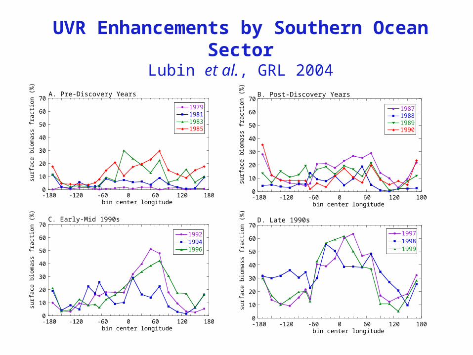
UVR Enhancements by Southern Ocean SectorLubin et al., GRL 2004

0

10

20

30

40

50

60

70

-180 -120 -60 0 60 120 180

1979198119831985

surf

ace

biom

ass

frac

tion

(%)

bin center longitude

A. Pre-Discovery Years

0

10

20

30

40

50

60

70

-180 -120 -60 0 60 120 180

1987198819891990

surf

ace

biom

ass

frac

tion

(%)

bin center longitude

B. Post-Discovery Years

0

10

20

30

40

50

60

70

-180 -120 -60 0 60 120 180

199219941996

surf

ace

biom

ass

frac

tion

(%)

bin center longitude

C. Early-Mid 1990s

0

10

20

30

40

50

60

70

-180 -120 -60 0 60 120 180

199719981999

surf

ace

biom

ass

frac

tion

(%)

bin center longitude

D. Late 1990s

Spectral Flux at the Sea Surface

• Edd and Edi are direct and diffuse components• surface reflection divided into direct and diffuse components,

both of which are sum of specular reflection and reflectance from sea foam

• sea foam reflectance a function of wind stress• Fresnel’s law for specular reflection

Ed (,0, t) 1 d Edd (,0 , t) 1 i Edi( ,0 ,t)

dr 0.5sin2( w )

sin2( w )

tan 2( w )

tan 2( w )

In-Water Optics

• Beer’s law for spectral flux penetration

• Diffuse attenuation coefficient Kd(z) partitioned into components describing attenuation by pure water, phytoplankton, detritus, and chromophoric dissolved organic matter.

Ed (z ) Ed (0 )e K (z)z

Kd (z) Kdw Kdp(z) KdDet(z) KdCDOM (z)

In-Water Optics - Components

Kdw(z) bbw(z) aw(z)

Kdp(z) bbp(z) ap

* (z)Chla(z)

KdDet(z) aDet (440, z)eS1( 400)

KdCDOM(z) aCDOM(400,z)eS2 ( 400)

•Pure Water: coefficents from Smith & Baker (1981)

•Plankton (chlorophyll) from Sathyendranath et al. (1989)

•Detritus from work by Arrigo et al. (1998)

•CDOM from work by Mitchell and Holm-Hansen (1991); Arrigo et al. (1998)

Phytoplankton Production

• G is phytoplankton growth rate (d-1) calculated from temperature and light availability

• C/Chl a is the phytoplankton C:Chl a mass ratio (50)

• Beff is effective phytoplankton concentration

• G is modeled in terms of a temperature-dependent maximum rate and a light limitation term

PP(z, t) G(z, t) CChla Beff (z, t)

G(z, t) G0ekT( z) 1 exp

PUR(z, t)

Ek

Cumulative Exposure to UVR

• Throughout the day, the physiological inactivation of algal biomass (effective biomass Beff) is expressed by reducing Beff with increasing UVR exposure.

• At dawn, Beff(z,t) is set = Chl a (z,t)

• Vertical mixing: simulated by averaging Beff over MLD, then applying this average to each layer within MLD

Beff (z, t) Beff (z, t t)e Hinh (z,t )

Hihn(z, t) A()Ed (, z, t)ddt280nm

700nm

t 0

t

Comparison with Field Observations:% decrease in C-fixation relative to no UVR

64 S, 72 W MODEL ICECOLORS

1979 1992 ozone hole 1990

Surface

+UVA+UVB 55 59 4 56-77+UVA 48 48 0 45-65+UVB 21 30 9 8-20

5 m depth

+UVA+UVB 40 43 3 35-80+UVA 36 36 0 15-42+UVB 11 16 5 21-60

Station A59.19 S, 56.89 E

04 October

1992, UVA+B1979, UVA+B1992, UVA1979, UVA1992, UVB1979, UVB

12:0012:3013:0013:3014:0014:3015:00

1992, UVA+B1979, UVA+B1992, UVA1979, UVA1992, UVB1979, UVB1992, No UV1979, No UV

12:0012:3013:0013:3014:0014:3015:00

0 0.05 0.10 0.15 0.20

0 0.05 0.10 0.15 0.200 0.05 0.10 0.15

Hinh Beff (mg Chl a m-3)

0

5

10

15

20

25

30

0

5

10

15

20

25

30

0

5

10

15

20

25

30

Beff (mg Chl a m-3)

0 0.5 1.0 1.5 2.0 2.5 3.0

Daily production (mg C m-3)

0

10

20

30

40

50

60

70

80

90

100

A B

DC

•Photoinhibition dose Hinh varies with time and depth, 30% greater in exp. run than control at surface

•Assess individual contributions of UV-B and UV-A

•Substantial UV-A contribution to Hinh and Beff

•Panel B: 1979 (control)

•Panel C: 1992 (exp.)

Total Change in Primary Production

Temporal Variation in Primary Production Loss

over Southern Ocean

-0.1

0.0

0.1

0.2

0.3

0.4

0.5

0.6

0.7

0

5

10

15

20

25

% loss in production

% decrease in ozone

R = 0.85

Aug Sep Oct Nov Dec

Date

0

50

100

150

200

250

300

350

1979

1992

A

B

Major Conclusion of Small Impact• Surface UVR-induced losses of primary production can be several percent,

with large UV-B component• When integrated to 0.1% light depth, loss of primary production throughout

Southern Ocean, due to enhanced UV-B, is < 0.25%• Major reasons: strong UV-B attenuation with depth, location of most ozone

depletion over Antarctic continent, temporal mismatch between maximum ozone loss and maximum phytoplankton abundance

• Several sensitivity analyses did not alter this conclusion:– changing MLD and mixing time– temperature dependence of primary production– Photoacclimation parameter Ek, specifying saturation of photosynthesis– detrital and CDOM absorption– phytoplankton absorption– variability in Action Spectrum– Instantaneous versus cumulative exposure to UVR

Necessary Future Work•Improve parameterizations throughout model

in-water radiative transfer, processes very near sea ice

•Repeat experiments for even deeper and longer-lasting ozone holes of late 1990s

•Consider regional ecosystem effects