assessing the supplier role of selected fresh produce

Assessing the Supplier Role of Selected Fresh Produce Value Chains in the United States

Houtian Ge

Department of Agricultural Economics, Sociology and Education

The Northeast Regional Center for Rural Development

Penn State University

[email protected]

Patrick Canning

Economic Research Service

U.S. Department of Agriculture

[email protected]

Stephan J. Goetz

Department of Agricultural Economics, Sociology and Education

The Northeast Regional Center for Rural Development

Penn State University

[email protected]

Agnes Perez

Economic Research Service

U.S. Department of Agriculture

[email protected]

Abstract: This article identifies through simulation analysis the optimal locations of regional

fresh produce assembly hubs in the U.S. In contrast to much of the literature, we introduce

economies of scale into the model and annual production statistics are disaggregated into four

seasonal segments to more accurately account for the highly variable geographic disposition of

annual fresh produce production. The hub optimization problem is formulated as a mixed integer

linear programming model with the objective of minimizing total costs associated with fresh

produce assembly and hub operations. Our results suggest that scale economies have a

significant effect on the optimal solutions of hub numbers, locations and sizes. This article

provides a replicable empirical framework to conduct impact and cost assessments for regional

and local food systems.

Key words: Operations research, facility location, optimization, simulation, fresh produce

The views expressed here are those of the authors, and may not be attributed to the Economic

Research Service, the U.S. Department of Agriculture, or Penn State University. Partial funding

under USDA NIFA grant no. 2011-68004-30057 and under a cooperative agreement with ERS is

gratefully acknowledged.

mailto:[email protected]

mailto:[email protected]

1

Introduction

Food insecurity is a serious challenge for millions of Americans (Coleman-Jensen, Nord and

Singh 2013), and interest among consumers and private and public decision makers in the

sustainability of food supply chains is increasing as domestic and worldwide population grows

(Nicholson, Gómez and Gao 2011). Consequently, the structure and optimization of key

agricultural supply chains is of growing importance (King et al. 2010).

The U.S. Department of Agriculture (USDA) administers or is examining a variety of policies

and programs to (i) accommodate the growing demand for food that accompanies population

growth, (ii) enhance food access and affordability for low-income communities, and (iii)

encourage sustainable growth of the food system. To accomplish these goals while also

benefiting food system participants, USDA seeks to strengthen regional and local food systems.

Developing regional food hubs is an important component of this strategy. In 2009, the USDA

launched the “Know Your Farmer, Know Your Food” initiative to strengthen the connection

between farmers and consumers while supporting local and regional food systems.

Demand for locally grown food has increased dramatically in the last decade (Jablonski, et al.

2011). As policymakers, researchers, and practitioners seek new opportunities to support food

security and rural development, interest in regional and local food systems continues to grow

(Boys and Hughes 2013; Brown and Miller 2008; Clancy 2010; King et al. 2010; Martinez et al.

2010; O'Hara and Pirog 2013). The role of small- and medium-scale producers in developing

local and regional food systems has attracted renewed attention especially, as their importance in

supplying food markets has gained recognition (Darby et al. 2008; Low and Vogel 2011).

Despite the purported potential of local food systems to increase farm sales, particularly for

small and mid-scale producers, and support rural economic development, producers face a lack

of distribution infrastructure and services and limited marketing capacity (Brown et al., 2014).

Many farmers and ranchers – especially smaller operations – are challenged by the lack of

distribution and processing infrastructure of appropriate scale that would give them wider access

to retail, institutional, and commercial foodservice markets (Martinez et al. 2010). These small-

and medium-scale producers are too small to compete effectively in traditional wholesale supply

chains and often lack the volume and consistent supply needed to attract retail and foodservice

2

customers. Furthermore, due to limited staff or lack of experience, they are not always able to

devote the attention necessary to develop successful business relationships and linkages with key

wholesale buyers or have the resources to develop effective marketing strategies.

Regional food hubs are seen as an effective way to overcome these infrastructural and market

barriers and provide growers with cost-effective product consolidation and distribution (Low et

al. 2015; Tropp 2008). USDA’s Agricultural Marketing Service (AMS) defines food hubs as “a

centrally located facility with a business management structure facilitating the aggregation,

storage, processing, distribution, and/or marketing of locally/regionally produced food products.”

(www.ams.usda.gov/AMSv1.0/FoodHubs). For smaller and mid-sized producers who wish to

scale up their operations or diversify their market channels, food hubs offer a combination of

services that allows them to take advantage of the growing demand for locally and regionally

grown food in large volume markets that would be difficult or impossible to access on their own.

From this point of view, food hubs create new marketing opportunities for farmers and ranchers

to expand their markets, providing a critical supply chain link for rural communities and farmers

to reach consumers interested in purchasing local products.

This paper examines the roles and potential market impacts of regional food hub development

through consideration of assembly (as opposed to distribution) hub locations in selected fresh

produce value chains in the United States. Fresh produce suppliers -- comprising shippers,

importers, wholesalers, distributors, and brokers -- provide a range of marketing services for

domestic and international growers supplying fresh produce to U.S. markets, and to their retail

and foodservice customers serving the U.S. market (Cook, 2011). The annual U.S. retail value of

fresh produce reflects costs distributed roughly equally among the farm value, the value of

supplier services, and the value of services from retailing and foodservice establishments

(Canning 2011). Whereas research on and analysis of the production and retailing segments of

fresh produce value chains is extensive and produce assembler studies have been limited and

narrow in scope, leaving a gap in our understanding of these important value chains.

To narrow this gap, this research characterizes and models transportation and supplier logistic

(TSL) services in selected U.S. fresh produce markets, focusing on commodities that are highly

perishable (i.e., excluding commodities that can keep fresh in long term cold storage such as

3

apples and cabbage). We solve for both the scale and locations of these TSL hubs that minimize

total costs of assembling and distributing U.S. production to final markets. Outputs from this

model include assembler cost functions that characterize scale economies across fresh produce

TSL hubs, and shipping cost functions that characterize the impedance-based transportation costs

for shipments between production nodes and supplier hubs.

Literature Review

Hub-and-spoke networks have become an important field of discrete location research (Camargo

and Miranda 2012). Direct transportation of flows between pairs of origin-destination nodes is

usually extremely costly. As an alternative, flows from different origins but addressed to the

same destination can be consolidated at transshipment nodes, known as hubs, prior to be routed,

sometimes via other hubs, towards their destinations. Hubs are then responsible for flow

aggregation and redistribution. Hub location modeling is common in air transportation,

telecommunication, ground freight transportation and other transportation scenarios (Aros-Vera,

Marianov and Mitchel 2013; Horner and O’Kelly 2001; Dantrakul, Likasiri and Pongvuthithum

2014; Jouzdani, Sadjadi and Fathian 2013). These applications of hub location modeling in the

literature have shed light on network optimization and helped pave the way for a more complete

methodological framework to study hub network design.

In the past decade, growing attention has also been given to the need for and importance of

conducting more empirical studies related to the supply chain for local food products

(Abatekassa and Peterson 2011). In this area, the regional food hub concept has sparked strong

interest from a wide array of food system planners, researchers and policy makers. There exists a

substantial discussion in the literature regarding the role of regional and local food hubs in

improving market access for producers along with their potential for expanding the availability

of fresh food in communities, including underserved communities (Alumur and Kara 2008;

Campbel, Ernst and Krishnaoorthy 2002; Feenstra et al. 2011; Jablonski, Schmit and Kay 2015;

O’Hara and Pirog 2013). These data driven models were built with the goal to look for patterns

and practices that are consistent enough to be used as viable regional distribution solutions for

local food marketing.

4

Two recent studies by Etemadnia et al. (2013, 2015) formulate hub location problems as

mathematical programming models that minimize total network costs which include costs of

transporting goods and locating facilities. Computational experiments were conducted to identify

the optimal hub numbers and locations in food supply chain systems. While the method and

analysis contribute to the analysis of optimization of local food systems, these studies impose

strong simplifications on the operational level which are directly related to the solution of facility

location. First, they use annual production data and neglect seasonal differentials in production

which can affect the hub operational strategies- and generate heterogeneous costs across

marketing seasons. To effectively formulate the system patterns and structure, annual network

costs should be derived from the sum of components of seasonal costs. Second, they assumed

homogeneous operation costs across hubs with varying handling capacities. As an economic

phenomenon common in fresh supply chain system, economic scale effects play an essential role

in shaping the optimal network configuration. The lack of scale effects in the models means

generated solutions are likely to deviate from representative experimental conditions that ought

to be used to reach an optimum. This study relaxes these assumptions and develops more

realistic models that fit the supply chain context.

The Effects of Scale Economies

Economies of scale play a fundamental role in network design (Camargo, Miranda and Luna,

2009; Horner and O’Kelly, 2001). To understand the actual operating cost patterns and identify

empirical evidence of scale effects inherent in hub operations, we collect and analyze data on the

scope and scale of food hub operations. Based on 2007 Economic Census data regarding county

and state level fresh produce sale values and corresponding operational cost, we compiled data

for geotype=02 (state or equivalent) and 03 (county ) and obtained 108 observations. Four

hierarchy quartiles are defined based on sale values of hubs: 0.05-0.20 billion dollars, 0.2-0.5

billion, 0.5-1 billion and 1 billion above. For each quartile, the relationship between the hub

operation cost (independent variable (X)) and the sale value of the hub (dependent variable) is

regressed (Table 1).

5

Table 1. Regression Results for Scale Effect of Economies (Fresh Produce)

Quartiles Variables Coefficients t Stat P-value F R

Square

obs.

Quartile 1 Intercept 1068.4 0.235 0.816 48.35 0.659 27

X Variable 0.217**

6.954 0.000


X Variable 0.206**

4.729 0.000


X Variable 0.180**

4.163 0.0003


X Variable 0.176**

34.52 0.000

Note: **

significant at 5% level

The operational costs are broken into fixed and variable (or marginal) costs. Fixed costs include

hub establishment and maintenance, machinery, equipment and so on that are independent of

volume of products handled. They remain constant in a quartile. Variable costs include wages,

utilities and other sources of costs used in handling products. In these regressions, the fixed costs

are the intercept terms and the variable costs are the coefficients of variables. Regression results

show fixed costs (intercept) increase with the scale of hub, and on the contrary, the marginal

costs decrease with the scale of hub, i.e., the more products handled, the less the marginal cost

for one unit increase in the volume handled. The operational cost for per dollar sale value

handled is $0.217, $0.206, $0.180 and $0.176 from lower quartile 1 (with smaller sale value) to

upper quartile 4 (with larger sale value). In this manner, handling cost of a shipper hub is based

on the amount of product flow carried by the hub and is endogenously responsive to flow by

rewarding the shipper for greater volumes shipped. Under cost minimization principles, the

number and scale of facilities to be established typically becomes an endogenous decision. Based

on these regression results, this study embodies the economic scale effect into the models and

demonstrates how it leads to differing spatial network structures.

6

The Problem Statement and Methodology

The objective of this study is to identify and profile supplier roles of fresh produce value chains

and collect and analyze data on the scope and scale of supplier operations in order to more

clearly understand their potential role and impact in the U.S. food system. To do this, a model is

built to identify the optimal number, scale and locations for TSL hubs for fresh produce sourced

from growers located in multiple U. S. counties. We formulate the hub optimization problem as

a mixed integer linear programming model with the objective of minimizing total costs

associated with product assembly and hub operations. The optimization problem is subject to

constraints to ensure that total production by region and average per unit supplier and shipping

costs meet observed statistics. The following notations are introduced for the models.

I={1,2,3,4} denotes four marketing seasons in a year;

F={1,2,3…,f} denotes a set of production locations;

S={1,2,3,…,s} denotes a set of hub candidate locations;

c ∈ 𝐶 denotes capacity level of assembly hubs; each capacity level has an interval span;

𝑥𝑖,𝑓,𝑠 denotes quantity shipped from production location f to hub location f in marketing season i;

𝑝𝑖,𝑓 denotes production at production location f in marketing season i;

𝑧𝑐,𝑠 denotes an integer variable = 1 if location s is a hub with capacity c, and 0 otherwise;

𝑑𝑓,𝑠 denotes distance between production location f to hub location s (impedance miles) ;

t denotes fixed transportation cost ($ per thousand pound impedance mile);

DT denotes distance threshold between production locations and hub locations (impedance

miles);

𝑈𝑐,𝑠1 denotes maximum capacity of c level hub in location s;

𝑉𝑐,𝑠1 denotes minimum capacity of c level hub in location s;

𝑈𝑐,𝑠2 denotes maximum quantity of products handled at c level hub in location s during all

marketing seasons;

7

𝑉𝑐,𝑠2 denotes minimum quantity of products handled at c level hub in location s during all

marketing seasons;

TCs denotes total annual hub s operation costs, and

TC = ∑sTCs denotes annual hub operation costs nationwide.

A TSL hub facility of capacity c is costly to build and maintain. The annual opportunity costs of

equity financing, interest costs of debt financing, and replacement costs of physical and

economic depreciation are born by owners regardless of TSL services produced; denote these as

fixed setup and maintenance costs, ℎ𝑐0 . In addition, for each unit of produce handled up to the

capacity to which the hub facility is built, a per unit handling cost is incurred; denote these as

marginal costs, ℎ𝑐1. For any region s where a TSL produce hub facility of capacity c is located,

total handling charges from assembling commodities for distribution are:

1) 𝑇𝐶𝑠 = ℎ𝑐,𝑠0 + ℎ𝑐.𝑠

1 ∙ 𝑄𝑠

where Q,s = ∑i∊I ∑f∊F 𝑥𝑖,𝑓,𝑠 , and 𝑥𝑖,𝑓,𝑠 denotes the quantity of produce grown in production node

location f and shipped to hub s in marketing season i. Produce hub investors are assumed to

choose from a finite number, C, of possible hub capacities to build a TSL produce hub. Each hub

size has a maximum capacity constraint, ℎ𝑐𝑚𝑎𝑥, which determines the maximum quantity of

production that can be transported to the hub across four marketing seasons.

Produce assembly at hub location s involves shipments from surrounding production and import

regions (or nodes) via a domestic freight network that connects all nodes and hubs. All shipments

are assumed to be transferred by land using trucks, and the transportation cost is a function of

travel distance (impedance miles). This cost may be paid by the grower/importer or the supplier,

and is reflected in the fob supplier price1,

2) ∑ ∑ ∑ {𝑡 ∙ 𝑑𝑓,𝑠 ∙ 𝑥𝑖,𝑓,𝑠}𝑠∈𝑆𝑓∈𝐹𝑖∈𝐼 ,

where 𝑡 ∙ 𝑑𝑓,𝑠 is the unit transportation cost for shipments between growing/import node f and

hub location s.

1 Free-on-board (fob) supplier price is the unit cost that buyers of fresh produce from hub o are charged assuming

the buyer pays (or is charged separately) all freight costs to ship their purchase to the buyers location.

8

Transportation costs between node pairs are usually defined to be proportional to the distance

between nodes. However, transportation costs are also subject to constraints, e.g., road condition,

speed reduced on evening commute, traffic jams and congestion which influence travel time and

speed (Novaco, Stokols and Milanesi 1990). This involves the concept of impedance. To

evaluate the transportation costs between production nodes and hubs, each link in the network is

assigned an impedance value other than actual mileage. Impedance represents a measure of the

amount of resistance, or cost, required to traverse a path in a network, or to move from one

element in the network to another. High impedance values indicate more resistance to

movement. For this study, we use version 3 of the national multi-modal impedance network

database (http://cta.ornl.gov/transnet/SkimTree.htm).

For a national fresh produce transportation and supplier logistics system, optimal TSL hub scales

and locations are determined by minimizing total costs of TSL hub operations plus shipping

costs of moving all domestically grown fresh produce to a TSL hub. The objective function and

system constraints of a model to solve this problem are given in equations 3 to 9.

Minimize

3) 𝑇𝐶 = ∑ ∑ {(ℎ𝑐,𝑠0 + ℎ𝑐,𝑠

1 ∙ 𝑄𝑠) ∙ 𝑍𝑐,𝑠}𝑠∈𝑆𝑐∈𝐶 + ∑ ∑ ∑ {𝑥𝑖,𝑓,𝑠 ∙ 𝑑𝑓,𝑠 ∙ 𝑡 }𝑠∈𝑆𝑓∈𝐹𝑖∈𝐼

Subject to:

4) ∑ 𝑥𝑖,𝑓,𝑠𝑠∈𝑆 = 𝑝𝑖,𝑓 ∀ 𝑖, 𝑓

5) 𝑍𝑐,𝑠 ∈ {1,0} ∀ 𝑐, 𝑠

6) ∑ 𝑍𝑐,𝑠𝑐∈𝐶 ≤ 1 ∀ 𝑠

7) ∑ 𝑥𝑖,𝑓,𝑠𝑓∈𝐹 ≤ ∑ 𝑍𝑐,𝑠𝑈𝑐,𝑠1

𝑐 ∀𝑖, 𝑠

8) ∑ 𝑥𝑖,𝑓,𝑠𝑓∈𝐹 ≥ ∑ 𝑍𝑐,𝑠𝑉𝑐,𝑠1

𝑐 ∀ 𝑖, 𝑐, 𝑠

9) ∑ ∑ 𝑥𝑖,𝑓,𝑠 ≤𝑓∈𝐹𝑖∈𝐼 𝑍𝑐,𝑠𝑈𝑐,𝑠2 ∀ 𝑐, 𝑠

10) ∑ ∑ 𝑥𝑖,𝑓,𝑠𝑓∈𝐹𝑖∈𝐼 ≥ 𝑍𝑐,𝑠𝑉𝑐,𝑠2 ∀ 𝑐, 𝑠

11) 𝑥𝑖,𝑓,𝑠 ≥ 0 ∀ 𝑖, 𝑓, 𝑠

http://cta.ornl.gov/transnet/SkimTree.htm

9

The objective function (3) minimizes total cost. Equation (4) ensures that in each marketing

season the total quantity transported from production region f to all hubs S are equal to total

quantity produced in region f in the season. That is, all products must be assembled into hubs

across marketing seasons. Equation (5) provides the binary condition—build/do not build, while

equation (6) guarantees that the total number of hubs built in hub location s is not more than 1.

Equations (7) and (8) ensure that products will not be transported to any hub location s unless a

hub is installed and there is sufficient capacity to handle all products transported to hub s in

marketing season i. Equations (9) and (10) define the quantity handling threshold for a hub to

enjoy a certain level of scale effect. Equation (11) ensures that shipments only flow from farms

to hubs and not vice versa.

Data

The National Agricultural Statistics Service (NASS) of the U.S. Department of Agriculture

(USDA) reports State level annual production statistics for 21 different fresh market vegetable

crops across 37 States (USDA/NASS, 2009). The 2007 statistics are allocated to counties in

these States based on harvested county acreage, using table 30 in the 2007 Census of Agriculture

(USDA/NASS, 2009b). For States not covered in the annual NASS reports but that are covered

in the Census, harvested acreage data from the Census are multiplied by yield per acre data in

nearby States to impute production. To overcome data suppressions in the Census data, a

constrained maximum likelihood mathematical programming model was used. The model

minimizes adjustments to the variance weighted initial estimates of suppressed data to align

these estimates with the adding up requirements of the hierarchical data in table 30. This

hierarchy includes requirements that the sum of harvested crop acreage across all commodities

equal the published county-wide total harvested vegetable acreage, and that the sum of harvested

acreage for specific crops across all counties in a State equal the published statewide total for

each crop. By simultaneously solving a State/County model and a National/State model for the

same commodities, the model produces maximum likelihood estimates of all suppressed county

harvested acreage statistics. The same approach was used for estimates of fresh market fruit

production in U.S. counties, based on annual production statistics of 34 different fresh market

fruit and berry crops across 43 States (U.S. Department of Agriculture, 2009c, 2009d), and tables

10

31 and 32 of the Census (USDA/NASS, 2009b). Combined production for the subset of these 55

crops produced in each county are converted to a common unit (1,000 lbs) and summed to a

single production statistic per county. County-to-county shipping costs are based on Oak Ridge

National Laboratory multi-modal impedance network data product, and average shipping costs

statistics published by AMS. Empirical estimates of fixed and per unit marginal handling costs

for each capacity choice are obtained from regression analysis of data in the Economic Census of

Wholesale Trade.

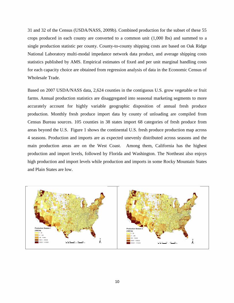
Based on 2007 USDA/NASS data, 2,624 counties in the contiguous U.S. grow vegetable or fruit

farms. Annual production statistics are disaggregated into seasonal marketing segments to more

accurately account for highly variable geographic disposition of annual fresh produce

production. Monthly fresh produce import data by county of unloading are compiled from

Census Bureau sources. 105 counties in 38 states import 68 categories of fresh produce from

areas beyond the U.S. Figure 1 shows the continental U.S. fresh produce production map across

4 seasons. Production and imports are as expected unevenly distributed across seasons and the

main production areas are on the West Coast. Among them, California has the highest

production and import levels, followed by Florida and Washington. The Northeast also enjoys

high production and import levels while production and imports in some Rocky Mountain States

and Plain States are low.

11

Source: Authors. In blank counties, no survey data are reported.

Experimental Setting, Results and Analysis

The models assume varying costs for establishing and maintaining hubs with different capacities

and different unit costs for handling products in those hubs. The capacity of a hub is the

maximum quantity that can be handled in any one of the four marketing seasons. Hubs with

larger capacity can handle a larger quantity of products than hubs with smaller capacity during

marketing seasons. It is assumed that a hub must handle a minimal level of product quantity to

achieve a certain level of scale effect. Four different thresholds for quantity of products handled

at hubs during four marketing seasons are defined and named as Quartiles 1-4 (unit: thousand

pounds):

Quartile 1: 100,000 and below

Quartile 2: 100,001-500,000

Quartile 3: 500,001-2,000,000

Quartile 4: 2,000,000 and above

Regression results reported in table 1 are incorporated into these model simulations, where they

inform alternative hypothetical hub cost parameters. Thus, annually attributed hub fixed costs

Figure 1: Distribution of Fresh Produce Production in the U.S. across Seasons

Note: Season 1 is January – March, Season 2 is April – June, etc.

12

(h0) for handling quantity defined in four quartiles are $80,000, $120,000, $240,000 and

$400,000 respectively in models allowing for varying scales of hubs across quartiles. Following

the regression pattern of operating cost in the previous section, hubs handling a higher quantity

of products enjoy lower variable handling costs. The marginal handling costs (h1) used in this

model are calibrated as a ratio of 10% of their counterparts in regressions (table 1). Our goal is to

test the sensitivity of the model solution to the scale effect and we are aware that the magnitude

of the marginal handling cost significantly influences the model solutions, and that these costs

will be calibrated in a future iteration of this research.

In order to identify the effect of scale economies on the optimal solutions of the problem, we

design five experimental models. We assume different values of the marginal handling costs for

each of five models: the marginal cost margins (marginal cost difference between two adjacent

quartiles) are $0, $0.5, $1, $1.5, $2 for models 1-5 respectively. The fixed costs and marginal

costs for hubs in each quartile in each model are list in Table 2:

Table 2. Fixed Costs and Marginal Costs for Hubs

Quartiles

Fixed Costs (US$)

Marginal Costs (US$/1,000 lbs handled by hub)

Models 1-5 Model 1 Model 2 Model 3 Model 4 Model 5

1 80,000 22 22 22 22 22

2 120,000 22 21.5 21 20.5 20

3 240,000 22 21 20 19 18

4 400,000 22 20.5 19 17.5 16

Using the model reported in equations (3) to (9) and the set of parameter values and data, model

simulations for models 1 to 5 allows us to generate data for the hub location problem. The

optimization problem is compiled in GAMS and solved using CPLEX. All computational

executions were performed on a High Performance Computing System. Next we present the

results of computational experiments and conduct our analysis.

The hub numbers at each quartile across models change significantly due to the scale effect. As

shown in Table 2, the hub numbers in quartile 1 are negatively related to the marginal cost

13

margin and, on the contrary, the hub numbers in Quartiles 3 and 4 are positively related to the

marginal cost margin. The hub numbers in Quartile 2 do not change consistently across models.

The locations and scales (capacity) of these hubs in each model are shown in Figures 1-5. The

hub capacity is presented by the maximum quantity of product handled across the four marketing

seasons.

Table 2. The Number of hubs at Each Quartile across Models

Model 1 Model 2 Model 3 Model 4 Model 5

Quartile 1 367 254 190 142 111

Quartile 2 139 130 148 145 132

Quartile 3 45 51 51 59 60

Quartile 4 12 31 34 36 38

Total 563 466 423 382 341

Figure 2. Hub Locations for Model 1 (constant marginal cost across quartiles)

14

Figure 3. Hub Location for Model 2


15


Figure 6. Hub Locations for Model 5

16

With the scale effect, hubs handling a larger quantity of products enjoy lower marginal handling

costs. The merging of smaller hubs into larger hubs leads to handling cost savings. As shown in

Figure 7, compared with Model 1, the total quantity handled in Quartiles 1-3 hubs decreases for

models with scale effect (Models 2-4) while the total quantity handled in Quartile 4 hubs

increases. Among models with scale effect, the total quantity handled in Quartiles 1-2 hubs

decreases with the magnitude of the marginal cost margin and meanwhile the total quantities

handled in Quartiles 4 increase with the marginal cost margin. The change in quantity handled in

Quartile 3 hubs remains ambiguous when the marginal cost margin increases.

It is not surprising that the average quantity handled in each quartile continuously decreases as

the marginal cost margin widens from Model 2 to Model 5 (Figure 8). In this study, we set

minimum and maximum capacity constraints for each quartile. As the marginal cost margin

between quartiles increases, the incentives to establish more hubs with larger capacity become

stronger. To obtain the full benefit of economies of scale, distribution of products among hubs

becomes strategic in order to reduce the handling costs. Figures 9-12 show the quantity handled

at each individual hub in each quartile across models (in ascending order). As Figures 10-12

show, the number of hubs meeting the minimum threshold to enter Quartiles 2-4 increases with

the marginal cost margin, so that the average quantity handled in Quartiles 2-4 hubs approach the

minimum threshold. Although the total quantity handled in Quartile 4 hubs increases from Model

1 to Model 5, the total quantity handled in these hubs increases at a lower rate than the increase

in the number of hubs in the same model. As a result, the average quantity handled in these

hubs drops when the marginal handling cost margin increases.

17

Figure 7. Total Quantity Handled at Each Quartile across Models

Qu

anti

ty (

10

00

lb)

Qu

anti

ty (

10

00

lb)

Figure 8. Average Quantity Handled at Each Quartile across Models

18

Figure 9. Quantity Handled at Quartile 4 Hubs across

Models Models

Hubs

Qu

anti

ty (

10

00

lb)

Figure 10. Quantity Handled at Quartile 2 Hubs across Models

hubs

Qu

anti

ty (

10

00

lb)

19

The marginal cost between quartiles provides incentives for transporting products longer in order

to build upper quartile hubs which take advantage of the scale effect. As shown in Table 3, the

transportation costs increase with the marginal cost margin between quartiles. There is a tradeoff

between increased transportation costs and handling costs saved as a result of the scale effect.

Our model is designed to determine the optimal balance.

Hubs

Figure 11. Quantity Handled at Quartile 3 Hubs across Models

Qu

anti

ty (

10

00

lb)

Hubs

Figure 12. Quantity Handled at Quartile 4 Hubs across

Models Models

Qu

anti

ty (

10

00

lb)

20

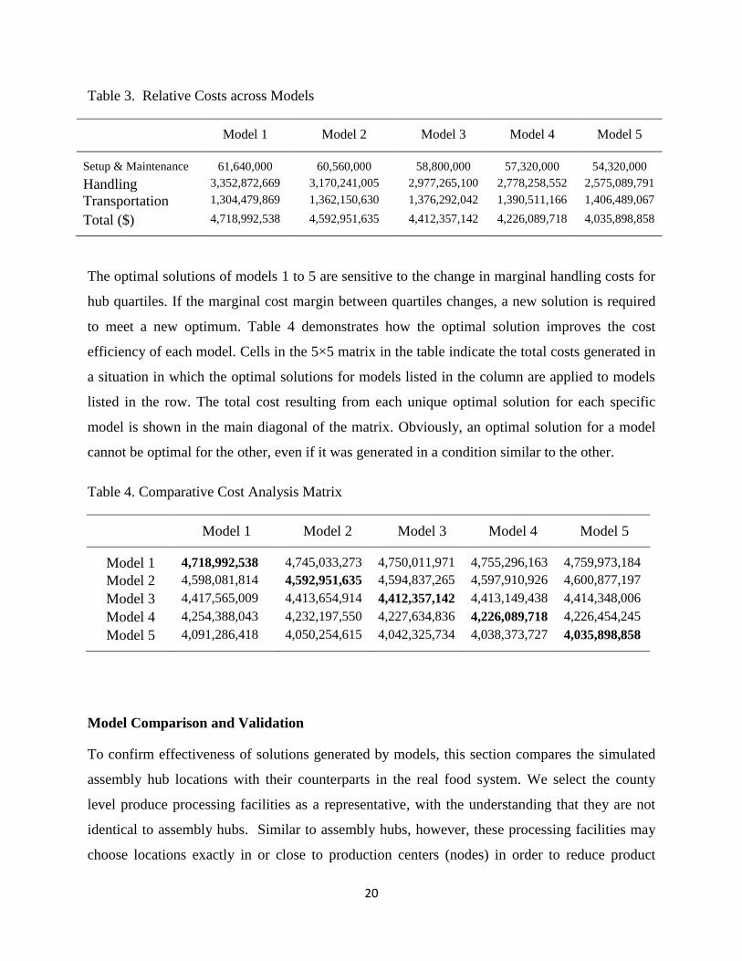
Table 3. Relative Costs across Models


Setup & Maintenance 61,640,000 60,560,000 58,800,000 57,320,000 54,320,000

Handling 3,352,872,669 3,170,241,005 2,977,265,100 2,778,258,552 2,575,089,791

Transportation 1,304,479,869 1,362,150,630 1,376,292,042 1,390,511,166 1,406,489,067

Total ($) 4,718,992,538 4,592,951,635 4,412,357,142 4,226,089,718 4,035,898,858

The optimal solutions of models 1 to 5 are sensitive to the change in marginal handling costs for

hub quartiles. If the marginal cost margin between quartiles changes, a new solution is required

to meet a new optimum. Table 4 demonstrates how the optimal solution improves the cost

efficiency of each model. Cells in the 5×5 matrix in the table indicate the total costs generated in

a situation in which the optimal solutions for models listed in the column are applied to models

listed in the row. The total cost resulting from each unique optimal solution for each specific

model is shown in the main diagonal of the matrix. Obviously, an optimal solution for a model

cannot be optimal for the other, even if it was generated in a condition similar to the other.

Table 4. Comparative Cost Analysis Matrix


Model 1 4,718,992,538 4,745,033,273 4,750,011,971 4,755,296,163 4,759,973,184

Model 2 4,598,081,814 4,592,951,635 4,594,837,265 4,597,910,926 4,600,877,197

Model 3 4,417,565,009 4,413,654,914 4,412,357,142 4,413,149,438 4,414,348,006

Model 4 4,254,388,043 4,232,197,550 4,227,634,836 4,226,089,718 4,226,454,245

Model 5 4,091,286,418 4,050,254,615 4,042,325,734 4,038,373,727 4,035,898,858

Model Comparison and Validation

To confirm effectiveness of solutions generated by models, this section compares the simulated

assembly hub locations with their counterparts in the real food system. We select the county

level produce processing facilities as a representative, with the understanding that they are not

identical to assembly hubs. Similar to assembly hubs, however, these processing facilities may

choose locations exactly in or close to production centers (nodes) in order to reduce product

21

transportation time and costs; from there, processed products are transported to distribution

centers or delivered directly to consumers. Due to their common characteristics and similar

functionalities, assembly hubs and processing facilities are comparable in terms their locations.

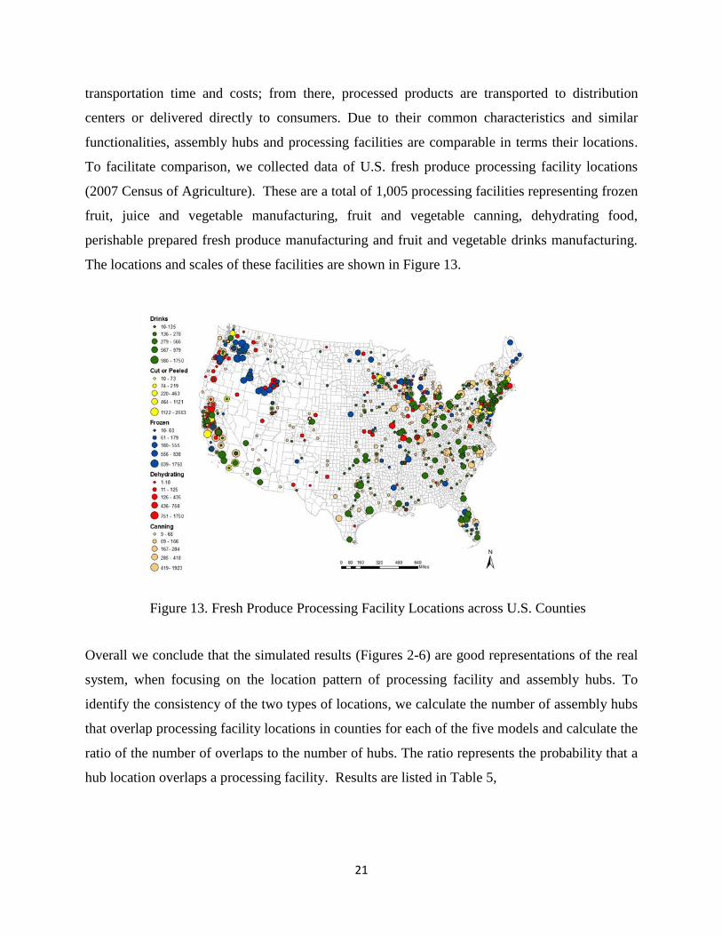
To facilitate comparison, we collected data of U.S. fresh produce processing facility locations

(2007 Census of Agriculture). These are a total of 1,005 processing facilities representing frozen

fruit, juice and vegetable manufacturing, fruit and vegetable canning, dehydrating food,

perishable prepared fresh produce manufacturing and fruit and vegetable drinks manufacturing.

The locations and scales of these facilities are shown in Figure 13.

Overall we conclude that the simulated results (Figures 2-6) are good representations of the real

system, when focusing on the location pattern of processing facility and assembly hubs. To

identify the consistency of the two types of locations, we calculate the number of assembly hubs

that overlap processing facility locations in counties for each of the five models and calculate the

ratio of the number of overlaps to the number of hubs. The ratio represents the probability that a

hub location overlaps a processing facility. Results are listed in Table 5,

Figure 13. Fresh Produce Processing Facility Locations across U.S. Counties

22

Table 5: Overlapping County Locations

Overlaps Hubs Ratio

Model 1 417 563 0.74

Model 2 404 466 0.87

Model 3 369 423 0.88

Model 4 342 382 0.91

Model 5 324 341 0.95

While there is a significant decrease in hub numbers from models 1-5, the number of overlapping

locations only slightly decreases. As a result, the overlap ratio increases from model 1 to model

5. Especially the ratio increases with a large margin from model 1 to model 2. There is a higher

ratio of location overlaps for models with scale effect than the model with no scale effect. The

models with scale effects better approximate the real system.

It is not surprising that our solutions do not perfectly duplicate and actual processing locations.

Based on the nature of the simulation, the divergence between them stems from the following

factors:

1. Our models are solved under certain assumptions about operational uncertainties, e.g.,

given requirement and constraints for hub operations, scale effects and transportation

cost. This study does not duplicate the environments which the real systems faced when

they emerged.

2. Our models are solved allowing for only economics incentives, but the real systems may

emerge under incentives beyond economic ones, such as social or political incentives.

The implemented optimization algorithms in this model do not address these possible

social or political characteristics inherent in real systems.

3. Our solutions are optimal but the real system may not be. Agriculture is undergoing

extreme change. The economic and operational environments keep evolving across time.

The agricultural supply chain system is actually vulnerable to the environment evolution.

23

Allowing for this, currently the real system may no longer be optimal, even if it once

was.

For the third reason, our model solutions may provide useful information to make improvements

in the overall efficiency of the logistics of the network.

Conclusions

Facility location is a well-established research area within operations research. The application

of hub location models has long been under discussion in regional and local food system studies

due to their presumed potential contribution to the sustainability of food supply chains. This

study provides a replicable empirical framework to conduct impact and cost assessments for

regional and local food systems. Overall the simulated results reflect the real system well.

We explore the idea of endogenous hub location on the fresh produce value chain. To overcome

limitations in the literature, we integrate an economy of scale effect into our models. By

collecting detailed expenditure and sales information from county statistics in the U.S., we

identify the pattern of scale effect inherent in hub operations and apply a cost of operation

function that rewards economies of scale on quantities handled in different hierarchy quartiles.

The hub optimization problem was mathematically formulated as a mixed integer linear

programming model with an objective to minimize the total costs associated with produce

assembly and hub operations. We designed several experiments to assess the scale effect of

economies in the network and visualized the results. Our results provide strong evidence that

scale effects have a significant impact on hub location solutions. Under different marginal cost

assumptions, produce transportation is re-routed to take advantage of cost saving, and thus the

structure of the network is reshaped. When the marginal handling cost margin increases between

a different hierarchy of hubs, more hubs with large capacity emerge while the number of small

capacity hubs diminishes.

Given the current policy environment, the research is timely and can provide valuable insights

into assessing the role and potential impacts of new regional food hub infrastructure investments,

as well as the costs and potential market outcomes of such investments. Such information is

24

currently lacking and is needed to help inform decisions of the various stakeholders interested in

regional food hub infrastructure investment.

Our model has several limitations that suggest topics for future investigation. Addressing scale

effect of economies by explicitly considering it as a cost in the objective function yields a more

realistic modeling approach. But specification of a suitable cost function allowing for scale

effects is not easy. In this study, empirical estimates of fixed and per unit marginal handling

costs for each capacity choice are informed by regression analysis of data based on a limited

number of observations and are based on a rough, initial classification. To fully advance the

modeling of these types of economic issues, more investigation is needed to better understand

the pattern of scale effect of economies and its influence on hub operation costs.

Our model only accounts for the early portion of the fresh produce supply chain, i.e., from the

point of origin to the point of assembly. Points of distribution and points of consumption are not

taken into consideration in the model. In this sense, the model abstracts from the actual U.S.

fresh produce value chain system and the complexity within it is reduced when compared to

reality. Incorporating all these components in a model helps to generate hub location solutions

that better mirror the actual set of decisions within the supply chain systems. Furthermore, based

on the nature of this study, the extension of seasonal production data to monthly production data

facilitates identifying the dynamics of the cycle of operating costs and helps generate solutions

more compatible with actual situation of fresh produce supply chain systems. Overcoming these

limitations can allow models to even more realistically simulate actual hub locations. We will

explore this in future research.

References

Abatekassa, G., and H.C. Peterson. 2011. “Market Access for Local Food through the

Conventional Food Supply Chain.” International Food and Agribusiness Management Review

14(1):63-82.

Alumur, S., and B.Y. Kara. 2008. “Network Hub Location Problems: The State of the Art.”

European Journal of Operational Research 190: 1–21.

25

Aros-Vera, F., V. Marianov and J. E. Mitchell. 2013. “p-Hub approach for the Optimal Park-and-

Ride Facility Location Problem.” European Journal of Operational Research, 226(2): 277- 285.

Boys, K.A., and D.W. Hughes. 2013. “A Regional Economics-Based Research Agenda for Local

Food Systems.” Journal of Agriculture, Food Systems, and Community Development 3(4):145–

150.

Brown, C. and M. Stacy. 2008. The Impacts of Local Markets: A Review of Research on

Farmers Markets and Community Supported Agriculture (CSA). American Journal of

Agricultural Economics 90(5): 1296-1302.

Brown J.P., S.J. Goetz, M.C. Ahearn and C. Liang. 2014. Linkages Between Community-

Focused Agriculture, Farm Sales, and Regional Growth. Economic Development Quarterly

28(1): 5-16.

Camargo, R.S., and G. Miranda. 2012. “Addressing Congestion On Single Allocation Hub-and-

Spoke Networks.” PesquisaOperacional 32(3):465-496.

Camargo, R.S., G. Miranda, and H.P.L. Luna. 2009. “Benders Decomposition for Hub Location

Problems with Economies of Scale.” Transportation Science 43(1):86–97.

Campbell, J.F., A.T. Ernst, and M. Krishnamoorthy. 2002. “Hub Location Problems.” In Z.

Drezner and H.W. Hamacher, 1st ed. Facility Location: Applications and Theory. Springer,

pp.373–407.

Canning, P. 2011. A Revised and Expanded Food Dollar Series: A Better Understanding of Our

Food Costs. Washington, D.C.: U.S. Department of Agriculture, Economic Research Service,

Economic Research, Rep. 114, February.

Coleman-Jensen, A., M. Nord, and A. Singh. 2013. Household Food Security in the United

States in 2012. Washington D.C., U.S. Department of Agriculture, Economic Research Service,

Economic Research. Rep. 155, September.

Cook, R. 2011. “Fundamental Forces Affecting U.S. Fresh Produce Growers and Marketers.”

Choices 26(4): 4th Quarter.

Darby, K., M.T. Batte, E. Stan and R. Brian. 2008. Decomposing Local: A Conjoint Analysis of

Locally Produced Foods. American Journal of Agricultural Economics 90(2): 476-486.

Dantrakul, S., C. Likasiri, and R. Pongvuthithum. 2014. “Applied p-median and p-center

Algorithms for facility Location Problems.” Expert Systems with Applications 41(8): 3596-3604.

Etemadnia, H., S.J. Goetza, P. Canning, and M.S. Tavallali. 2015. “Optimal Wholesale Facilities

Location within the Fruit and Vegetables Supply Chain With Bimodal Transportation Options:

An LP-MIP Heuristic Approach.” European Journal of Operational Research 244(2):648-661.

26

Etemadnia, H., A.Hassan, S. Goetz, and K. Abdelghany. 2013. “Wholesale Hub Locations In

Food Supply Chain Systems.” Journal of Transportation Research Board. 2379:80-89..

Feenstra, G., P. Allen, S. Hardesty, J. Ohmart, and J. Perez. 2011. “Using a Supply Chain

Analysis to Assess the Sustainability of Farm-to-Institution Programs.” Journal of Agriculture,

Food Systems, and Community Development 1(4):69-85.

Horner, M.W., and M.E. O’kelly. 2001. “Embedding Economies of Scale Concepts for Hub

Network Design.” Journal of Transport Geography 9(4):255-265.

Jablonski, B.B.R., J. Perez-Burgos, and M.I. Gómez. 2011. “Food Value Chain Development in

Central New York: CNY Bounty.” Journal of Agriculture, Food Systems, and Community

Development 1(4):129–141.

Jablonski, B.B.R., T.M. Schmit, and D. Kay. 2015. “Assessing the Economic Impacts of Food

Hubs to Regional Economies: a framework including opportunity cost.” Working Paper, Charles

H. Dyson School of Applied Economics and Management, Cornell University, Ithaca, New

York, USA.

Jouzdani, J., S.J. Sadjadi, and M. Fathian. 2013. “Dynamic Dairy Facility Location and Supply

Chain Planning under Traffic Congestion and Demand Uncertainty: A Case Study of Tehran.”

Applied Mathematical Modelling 37(18-19):8467–8483.

King, R., M. Boehlje, M. Cook, and S. Sonka. 2010. Agribusiness Economics and Management.

American Journal of Agricultural Economics 92(2): 554-570.

King, R., M.S. Hand, G. DiGiacomo, K. Clancy, M.I. Gómez, S.D. Hardesty, L. Lev, and E.W.

McLaughlin. 2010. Comparing the Structure, Size, and Performance of Local and Mainstream

Food Supply Chains. Washington, D.C.: U.S. Department of Agriculture, Economic Research

Service, Economic Research, Rep. 99, June.

Low, S., A. Adalja, E. Beaulieu, N. Key, S. Martinez, L. Melton, A. Perez, K. Ralston, H.

Stewart, S. Suttles and S. Vogel. 2015. Trends in U.S. Local and Regional Food Systems: A

Report to Congress. Washington, D.C.: U.S. Department of Agriculture, Economic Research

Service, Economic Research, Rep. 68, January.

Low, S.A., and S. Vogel. 2011. Direct and Intermediated Marketing of Local Foods in the

United States. Washington, D.C.: U.S. Department of Agriculture, Economic Research Service,

Economic Research, Rep. 128, November.

Martinez, S., M. Hand, M.D. Pra, S. Pollack, K. Ralston, T. Smith, S. Vogel, S. Clark, L. Lohr,

S. Low and C. Newman. 2010. Local Food Systems: Concepts, Impacts, and Issues. Washington

DC: U.S. Department of Agriculture, Economic Research Service, Economic Research, Rep. 97,

May.

27

Nicholson, C.F., M.I. Gómez, and O.H. Gao. 2011. “The Costs of Increased Localization for a

Multiple-Product Food Supply Chain: Dairy in the United States.” Food Policy 36(2):300–310.

Novaco, R.W., D. Stokols, and L. Milanesi. 1990. “Objective and Subjective Dimensions of

Travel Impedance as Determinants Of Commuting Stress.” American Journal of Community

Psychology 18(2):231-257.

Oak Ridge National Laboratory, Center for Transportation Analysis website


O’Hara, J., and R. Pirog. 2013. “Economic Impacts of Local Food Systems: Future Research

Priorities.” Journal of Agriculture, Food Systems, and Community Development 3(4): 35-42.

Tropp D. 2008. The Growing Role of Local Food Markets: Discussion. American Journal of

Agricultural Economics 90(5): 1310-1311.

U.S. Department of Agriculture.2009a. Vegetables–2008 Summary, NASS Vg 1-2(09),

Washington DC, January.

U.S. Department of Agriculture. 2009b. United States Data (Chapter 2) in 2007 Census of

Agriculture, NASS, Washington DC, February.

U.S. Department of Agriculture. 2009c. Noncitrus Fruits and Nuts-2008 Summary. NASS Fr Nt

1-3(09). Washington DC, May.

U.S. Department of Agriculture. 2009d. Citrus Fruits–2009 Summary. NASS Fr Nt 3-1(09),

Washington DC, May.


assessing the supplier role of selected fresh produce

Documents