assessment of flutter speed on long span bridges...assessment of flutter speed on long span bridges...

Assessment of flutter speed on long span bridges

M. Papinutti1, J. Kramer Stajnko1, R. Jecl1, A. Štrukelj1, M. Zadravec2 & J. Á. Jurado3 1Faculty of Civil Engineering, University of Maribor, Slovenia 2Faculty of Mechanical Engineering, University of Maribor, Slovenia 3School of Civil Engineering, University of Coruña, Campus de Elviña, Spain

Abstract

In this paper it is shown how to calculate flutter speed on the example of the Great Belt East Bridge in Denmark. Two numerical approaches are shown for prediction of the aeroelastic phenomena on bridges. In the computational fluid dynamics (CFD) simulation turbulence model based on Reynolds Average Navies Stokes (RANS) approach, two-equation shear stress turbulence (SST) models were chosen. Although the SST model needs more computer resources compared to the k-ω and k-ε models, it is still affordable with multi-processing personal computers. In this paper extracted flutter derivatives in the force vibration procedure are shown. Flutter derivatives are later used in the hybrid method of flutter. Final flutter speed was calculated based on flutter derivatives from fluid structure interaction extraction and experimental extraction. Flutter velocity was also determined with a free vibration of deck at the middle of the bridge. The deck section of unit length was clamped into springs and dampers. Flutter speed was reached with time increasing of wind speed until large oscillations occurred. The general procedure of how to formulate the fluid structure interaction and necessary stapes for flutter analysis of the bridge is shown in this paper. Numerically extracted flutter derivatives are compared based on the final flutter speed to experimental measurements of the deck section. Keywords: bridge aeroelasticity, long span bridge, flutter derivatives, numerical simulation, fluid structure interaction, computational fluid dynamics.

Fluid Structure Interaction VII 61

www.witpress.com, ISSN 1743-3509 (on-line) WIT Transactions on The Built Environment, Vol 129, © 2013 WIT Press

doi:10.2495/ 3FSI1 00 16

1 Bridge aeroelasticity

The aeroelastic stability of line-like slender structures, such as suspension and cable-stay bridges is verified by calculating the critical wind speed. Light structures are sensitive to aeroelastic phenomena like galloping, divergence and flutter. Therefore the aeroelastic properties of the bridge deck section are needed and are commonly determined in wind tunnel tests. The bridge structural parameters have to be calculated and, furthermore, more aeroelastic parameters must be measured. The phase of projecting flutter speed can be estimated fully with a computational approach. In general, aeroelastic studies are time consuming and quicker calculations could be done with fluid structure interaction (FSI) analysis. For an aeroelastic response in the hybrid method we need linearized flutter derivatives to close dynamic equations and the dynamic response of structure. The hybrid method is a very useful tool for optimization, sensitivity analysis and flutter speed calculations. A multimodal response could be captured, but in our example we captured only the vertical and torsional degree of freedom. Two different methods exist for the extraction of flutter derivatives – free and forced vibration testing. For our investigation, the force vibration test was simulated with commercial software Ansys 14 for computational fluid dynamics (CFD). A presentation of extraction of flutter derivatives will be presented by FSI simulation with a force vibration test. Results of flutter derivatives will be imported into the hybrid method for calculating the flutter speed. The second possibility is to cut a unit length of bridge deck segment at one-quarter or one-half of the bridge and investigate the aeroelastic response. We clamped the segment in springs, dampers and assigned a proper modal mass for chosen frequencies. Under different wind velocities we observed oscillations of the deck. Independent from hybrid results in frequency domain, a time domain FSI was calculated for the clamped deck section.

2 Flutter

It is shown that the fundamental torsional vibration mode dominantly involves flutter instability for bluff cross sections like low slenderness ratio (B/D) rectangular sections or H-shape sections or stiffened truss sections. The flutter instability [1] is known as the torsional flutter, as in the case of Tacoma Narrow failure, whereas the fundamental torsional mode and any first symmetric or asymmetric heaving mode usually couples mechanically at single frequency with the streamlined cross sections known as the coupled flutter or the classical flutter. Coupled flutter was studied previously on the aerodynamics of airplane’s airfoil wings and later developed for bridge line-like structures. It is interesting that the coupled flutter has occurred in the case of the Great Belt East Bridge in Denmark with a streamlined deck section. The following section will describe basic equations of flutter, based on which later flutter speed is calculated.

62 Fluid Structure Interaction VII


2.1 Equations of flutter

Aeroelastic forces are linearized as a function of the movements and speeds of the board, analogously to the forces occurring in the Theodorsen theory [2]. The expressions for lift and the moment forces are

12

(1)

12

(2)

where is the average wind speed, is the width of the section, ρ is the density of air and / is the reduced frequency. Circular frequency is 2 in units / and the frequency units are in 1/ . So called flutter derivatives , with 1 . . . 4 are functions of reduced frequency . Moment force , along the X-axis which produces torsional rotation along the deck. Lift force causes lift of the deck and is important for flutter coupling between the rotational and vertical movement. Drag forces are neglected for simplification and small participation factors to flutter speed, but can be important for long suspension [3]. Classical flutter occurs when vertical and torsional vibrations have natural frequencies close together and a larger mass is activated in each mode shape. Heaving and torsional motion equations of the flutter, where is the vertical motion and the torsional motion can be expressed with following

z t z t z t12

(3)

θ t θ t θ t 12

(4)

where is mass, is structural damping and is stiffness of mode i. Introducing / , non-dimensional time variable , first order

and second-order differentials of time we get equations of flutter

22 2

1z

2 2θ 0

(5)



2 21z

(6)

2 K2 2

θ 0

The solution of the system is in determining which must be zero. The determinant of eqns (5) and (6) can be expanded and grouped by real and imaginary parts as follows

Det Δ Δ 0 (7)

As a result, the flutter motion differential equations of the heaving-torsional system have been transformed to two polynomial equations with ω-variable. The critical state of circular frequency or flutter frequency is when the sum of real and imaginary parts are zero [4].

2.2 Extraction of flutter derivatives by force vibration procedure

Considering flutter as an aeroelastic stability problem, the motion of the bridge deck at the stability border is assumed to be a sinusoidal motion with constant amplitude. For forced vibration tests of the unit length deck, a smaller scale is used. Pure sinusoidal oscillation according to the mathematical assumption can be realized. The bridge deck involves two types of deformation: bending and twist. Based on the analytical theory of Theodorsen, a modified theory is introduced by Starossek [5, 6]. Mathematical expressions are used for determination of modal parameters [7, p. 34]. The harmonic behaviour of the system is introduced, by the use of expression for sinusoidal motion and exponential damping in

yzθ

y

z

θ

(8)

where is the sinusoidal lateral motion [m], the vertical sinusoidal motion [m] and is the rotation [m], is the frequency [rad], is the time variable [s] and y, z and θ are amplitudes of lateral, vertical and rotational movement. The forces described by the lift and moment coefficients are expected to vary in a similar way. A phase difference, between the motion and the load ψ is described by phase angle [rad] in eqns (9) and ((10).

z θθ

z

(9)

z θθ

z (10)



Phase angles are between 0 ψ π/2 and are calculated based on the fitted sinusoidal curve to each deck force and later phase difference between the sinusoidal motion and movement is calculated in eqn. (11).

Im

Imθ

Reθ

(11)

Re

Imz

Imθ

Reθ

Rez

2.2.1 Phase angle The phase angle is the delay of the load from motion. Load and motion are correlated as expected, as a positive clock wise rotation results in a positive moment and an upward lift (Figure 1). The time interval found in this particular case (in Figure 2) is approximately 0.35 rad for the lift and 0.12 rad for the moment. The phase difference is converted from time interval to radians as [7, p. 32] (eqn. (12)).

Figure 1: Global coordinate system of the bridge (left), Scalan sign convention used in the analysis of the flutter instability (right).

Figure 2: Lift force and vertical oscillation for illustration of the phase shift for the case with a reduced velocity 10 for force oscillation of frequency 0.129 1/ and wind speed 80 .

V

Fy y

z

Fz

θ F

Z

Y

V

ZX

Y



2

(12)

where is the time interval of the phase shift. Considering equation (11), the unknown is the phase shift ψ, which can be found with the time interval between the motion and the load as shown in Figure 3.

Figure 3: Aerodynamic forces for vertical oscillation z 15 m, 10, 0.129 1/s, 80 m/s.

In the example flutter derivatives for vertical motion , , , and for rotational motion , , , as a function of reduce frequencies K are calculated. Two different amplitudes were used for vertical force motion z0.05 m and z 0.15 m. For rotation, θ 5° and θ 15° are used and compared with different phase angles. It is of main importance to calculate phase angels and derivatives. Results for the four most important flutter derivatives are shown in Figure 4. Furthermore, phase angles are listed in Table 1 and the differences between amplitudes are shown in Table 2.

Table 1: Phase shifts ψ for rotational oscillation θ 5° and vertical oscillation z 5 cm.

Reduce frequency K 1 3 6 10 15 Frequency of oscillation 1,290 0,430 0,215 0,129 0,086

Lift Rotational oscillation θ 5°

1,03 0,95 0,65 0,35 0,19 Drag -0,51 -0,26 0,05 0,16 0,19 Moment 0,39 0,17 0,16 0,12 0,09 Lift Vertical

oscillation z 5 cm

0,27 0,76 1,35 1,46 1,43 Drag -1,44 -1,58 -1,38 -1,37 -1,39 Moment -1,54 -1,54 -1,45 -1,44 -1,46

2.2.2 Aerodynamic coefficients

Aerodynamic coefficients are calculated in the first stage of CFD simulations. Aerodynamic coefficients for stationary and non-stationary simulations are very similar but not the same. Usually the stationary solution underestimates forces on



Table 2: Difference for different amplitudes of rotational θ /θ and vertical z /z oscillation in % .

Reduce frequency K 1 3 6 10 15

Lift Rotation

-8,79% 0,15% -0,21% -0,67% -1,39% Drag 12,29% -2,44% 4,99% -2,74% -2,17% Moment 28,77% 0,77% -0,19% -0,13% -0,01% Lift

Vertical -40,65% 0,88% 0,05% 0,04% 7,08%

Drag 1,25% 0,14% 0,34% -0,02% -8,70% Moment 0,00% 0,00% 0,00% 0,00% 0,00%

Figure 4: Extracted flutter derivatives from experiments and FSI calculated by force vibration test.

deck. Aerodynamic non-stationary coefficients are the result of average force in time. For our investigation, aerodynamic forces on deck are calculated from stationary simulation. The drag aerodynamic coefficient 0.044, lift aerodynamic coefficient 0.197 and moment aerodynamic coefficient 0.050 are calculated from forces on the deck section at wind speed 80 / .

2.3 Flutter derivatives

The results are validated by comparison with wind tunnel tests, from ref. [8], focusing on the two-dimensional case. It is evident that amplitude does not significantly influence the results; it mostly influences the drag force. Instabilities of extraction were noticed also at higher amplitudes of rotations, where the vortex from leading travelling along the deck influenced the results. Flutter derivatives are compared to experimental data and it is possible to observe good agreement. The results are shown in Figure 4. Better agreement can be reached with a 3D mesh, denser mesh and another more accurate turbulence model.

-2

0

2

4

6

0 5 10 15

K=V/ωB

A2-expA3-expA2-FSIA3-FSI

-12

-10

-8

-6

-4

-2

00 5 10 15

K=V/ωB

H1-expH4-expH1-FSIH4-FSI



3 Direct simulation of fluid structure interaction of flutter

Different possibilities of moving meshes are possible to define rigid body motion. Two examples of the mathematical model are shown in Figure 5.

Figure 5: Different models for FSI analysis. Model for flutter derivatives extraction (left), direct FSI simulation of flutter (right).

3.1 Turbulence model

In RANS equations instantaneous fluctuations are modelled by a closure model. The most popular are the one and two equation models that are computationally cheap. The most economic approach is RANS flow modelling for computing complex turbulent industrial flows. RANS models are suitable for many engineering applications and typically provide the level of accuracy required. Since none of the models is universal, the most suitable turbulent model is an important decision in a given application. It influences the aerodynamic force which strongly influences the mechanism of energy transfer into motion, while the dynamic turbulence force from vortex shedding does not have a big influence on flutter. More complex RANS is the shear stress turbulence (SST) model. The transition SST model is based on the coupling of the SST transport equations

I N L E T

Mesh motion of rigid body

Deformable mesh

O U T L E T

Inflation layer Inflation layer

Rigid body-deck

Fixed mesh

Mesh motion of rigid body

I N L E T

O U T L E T

Rigid body-deck

Mesh motion of rigid body Mesh motion of rigid body

Deformable mesh Deformable mesh

Deformable mesh



with two other transport equations; one for the intermittency and one for the transition onset criteria, in terms of the momentum-thickness Reynolds number. An ANSYS empirical correlation covers standard bypass transition as well as flows in low free-stream turbulence environments. In addition, a very powerful option is included to allow us to enter our own user-defined empirical correlation. It was used to control the transition onset momentum thickness Reynolds number equation, which was used to match results of flutter derivatives. The mesh of our investigation is three-dimensional, while boundary conditions are set in a way that the symmetry condition defines equations to solve two-dimensions which is computationally cheaper [9]. Computation time is cheaper for 2D mesh and does not have a big influence for a line-like structure computed in RANS models.

3.2 Mathematical model of FSI

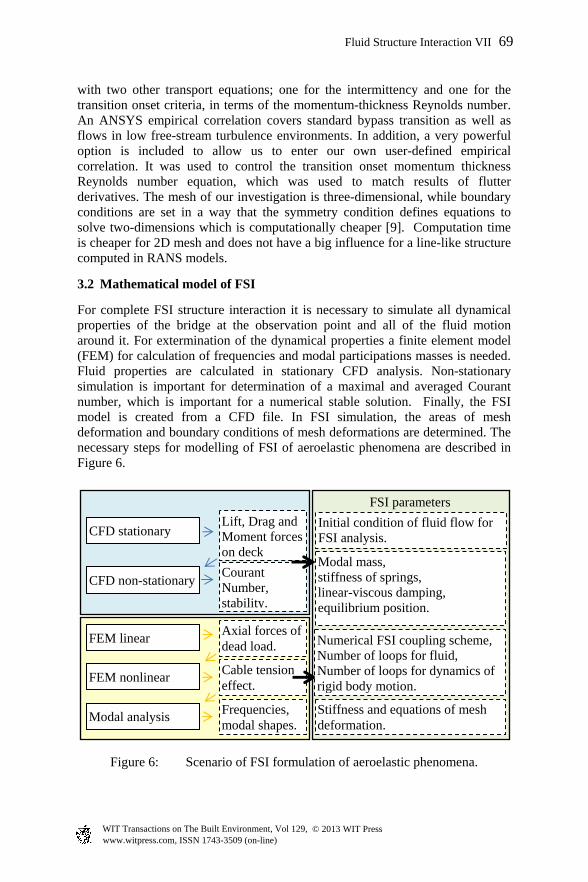
For complete FSI structure interaction it is necessary to simulate all dynamical properties of the bridge at the observation point and all of the fluid motion around it. For extermination of the dynamical properties a finite element model (FEM) for calculation of frequencies and modal participations masses is needed. Fluid properties are calculated in stationary CFD analysis. Non-stationary simulation is important for determination of a maximal and averaged Courant number, which is important for a numerical stable solution. Finally, the FSI model is created from a CFD file. In FSI simulation, the areas of mesh deformation and boundary conditions of mesh deformations are determined. The necessary steps for modelling of FSI of aeroelastic phenomena are described in Figure 6.

Figure 6: Scenario of FSI formulation of aeroelastic phenomena.

Simulation FSI parameters

Initial condition of fluid flow for FSI analysis.

Modal mass, stiffness of springs, linear-viscous damping, equilibrium position.

Stiffness and equations of mesh deformation.

CFD stationary Lift, Drag and Moment forces on deck

CFD non-stationary Courant Number, stability.

FEM linear Axial forces of dead load.

Modal analysis

Cable tension effect.

FEM nonlinear

Frequencies, modal shapes.

Numerical FSI coupling scheme, Number of loops for fluid, Number of loops for dynamics of rigid body motion.



Simulation is made at /2 of the main span of the bridge. The model is simplified for a coordinate system of rigid body movement. The centre of mass and shear centre are the origin of the shear centre. The origin of inertia forces, spring forces, damping and aerodynamic forces are calculated on the origin of the coordinate system in the shear centre. A system of two degrees of freedom is simulated with rigid body formulation in Ansys CEL language; modal mass, viscoelastic damper, and linear spring are defined in Figure 7. The results in Figure 8 are updated each time, when the fluid flow is calculated, rigid body deformation is calculated in the next loop.

Figure 7: Mathematical model programmed in Ansys CEL language.

Figure 8: Aeroelastic response of the deck at the midpoint of the bridge.

Large oscillations occur when the wind speed is around 80 m/s. Large rotational and vertical movements occur until the mathematical model becomes unstable. Instability occurs when one of the control cells has negative volume and a simulation is stopped.

-6

-4

-2

0

2

4

6

Spe

ed

[m

/s]

Time [s]

Angular velocity of the Deck

75 m/s60 m/s 65 m/s 70 m/s 80

Spring elastic force

Mass inertia force

Structural damping

Aeroelastic damping

Resultant damping force

1 DOF forces on system

6.00 m Rigid deck section

13.50 m

3.00 m

1.33 m

S. C.

C. G.

3.06 m 2.35 m

9.50 m9.50 m

Kz vertical springand ξz damper

Lift balance

≡S. C.≈ C. G.

Balance moment

z

y

Kθ rotational spring and ξθ damper

Mass

2 DOF FSI mathematical model



3.2.1 Finite element model FEM was made in software SAP2000. Cables, pylons and deck were modelled as line elements. Cable deformation for dead load was calculated with a SAP cable wizard program. Second order analysis was used for proper catching of the tension stiffening effect of the main cables. Because stiffness was calculated on a deformed FEM model it is not correct. To match correct stiffness pre-tensioning of main cables at the original position is done, so that dead load displacement is zero. Dynamical properties are considered in Figure 9 for investigation of first symmetric vertical mode 0.602 rad/s and first symmetrical torsional mode is 1.836 rad/s. At the centre of the bridge the first symmetrical vertical and first symmetrical torsional modes were investigated at the 1 m weight deck section.

Figure 9: First symmetrical vertical mode 2 and symmetrical torsional mode 39.

Masses and springs for fluid structure interaction are calculated from the FEM model. The modal mass is calculated for the unit length of FSI analysis 1 . The FEA model has a span between the two nodes 25.38 . Spectral displacement normalized on mass matrix from eigenvectors gives an activated mass at i-degree of freedom

m (13)

4 Results and conclusion

In this paper all steps of evaluating flutter speed were presented. The main question was the critical wind speed for this system. Our main goal was to apply advanced numerical programs for fluid structure interaction to asses flutter speed. An example of the Great Belt East Bridge was investigated to compare results of the two different methods. The critical wind speed was calculated in three different ways. The result of flutter derivatives from the experimental data was compared to FSI calculated flutter derivatives and the final result of flutter speed. The third way was the FSI analysis with the ANSYS software. The wind speed was increased step-by-step until the critical wind speed was found. Alternatively, considering the complexity of the problem, an approximation of 2D mesh and section in the middle of the bridge as rigid-body formulation was

2D cut



investigated. First, the aerodynamic derivatives were extracted from a 2D CFD simulation and the critical wind speed was evaluated using an updated method afterwards. The critical wind speeds obtained with three different methods are in good agreement. The results of FSI simulation show a slightly lower value of wind speed, which seems to be good coincidence in this complex simulation. Naturally, the inflow velocity steps should be more accurate in order to capture the flutter speed more precisely. In addition to that, the 2D mesh should be extended into the 3D mesh. Also multimodal response should be captured for a correct estimation of flutter speed. Furthermore, the method has potential for the evaluating of flutter speed in phase of construction where no experimental data are available. Extraction of flutter derivatives is in good agreement with the experimental data. Critical wind speed from flutter derivatives from wind tunnel testing gives flutter speed 91m/s and flutter derivatives from FSI extraction gives final wind speed 97 m/s. Flutter speed from direct FSI analysis is around 80 m/s.

Acknowledgements

We are deeply grateful to Profs S. Hernandez, J. Á. Jurado and their colleagues from the University of La Coruña in Spain for their help. M. Papinutti owes his most sincere gratitude to his mentors J. K. Stajnko and A. Štrukelj for all their support.

References

[1] Matsumoto, M., Shirato, H., Yagi, T., Shijo, R., Eguchi, A., Tamaki, H., Effects of aerodynamic interface between heaving and torsional vibration of the bridge decks: the case of Tacoma Narrows Bridge, Journal of Wind Engineering and Industrial Aerodynamics, 1547–1557, 2003.

[2] Scanlan, R.H., Airfoil and bridge deck flutter derivatives. Journal of Engineering Mechanics Division, ASCE. 97, 6, 1990.

[3] Jurado J. Á., Hernández, S., Theories of Aerodynamic Forces on Decks of Long Span Bridges. J. of Bridge Eng. 5, n1 8–13, 2000.

[4] Le, T.H., Nguyen, D.A., Bridge aeroelasticity in frequency domain. Airfoil and bridge deck flutter derivatives, 1992. http://uet.vnu.edu.vn /~thle/Bridge%20aeroelastic%20analysis_notsubmit.pdf

[5] Starossek, U., Brueckendynamik, Vieweg, Braunschweig/Germany. [6] Starossek, U., Prediction of bridge flutter through use of finite elements.

Structural Engineering Review, Vol. 5, No. 4, pp. 301–307, 1993. [7] Kenneth, S., Robert, S. Investigation on Long-span suspension bridges

during erection, The Great Belt East Bridge, p. 34. [8] Tanaka H., Aeroelastic stability of suspension bridges during erection.

Structural Engineering International. Journal of the International Association for Bridge and Structural Engineering (IABSE). Vol. 8, No. 2, pp. 118–123, 1998.

[9] Ansys help tutorial for CFX 14, Ansys software for multiphasic computational dynamics, 2012.



assessment of flutter speed on long span bridges...assessment of flutter speed on long span bridges...

Documents