asset substitution, debt overhang, and optimal capital ... · asset substitution, debt overhang,...
TRANSCRIPT
Asset Substitution, Debt Overhang, and Optimal Capital Structure
by
Jyh-Bang Jou1, and Tan (Charlene) Lee2
1 Massey University Albany Campus, Department of Economics and Finance, North Shore
City, 0745, New Zealand, phone: 64-9-4140800 ext. 9429, fax: 64-9-4418156, e-mail: [email protected].
2 Auckland University of Technology, Department of Finance, Auckland 1142, New Zealand, phone: 64-9-921-9999 ext. 5051, fax: 64-9-921-9940, e-mail: [email protected].
1
Asset Substitution, Debt Overhang, and Optimal Capital Structure
Abstract
This article uses a contingent-claims valuation method to compare debt financing,
investment, and risk choices of a firm adopting the second-best strategy with those of a
firm adopting the first-best strategy. The former bears the agency costs, as conjectured by
Jensen and Meckling (1976) and Myers (1977), because it chooses suboptimal investment
timing and risk levels, while the latter is able to avoid them. For plausible parameter values,
we find that the second-best firm that takes on more debt will under-invest and bear
excessive risk. We also find that the agency costs of debt are 15.8% of the first-best firm
value, which is higher than that found by Leland (1998) and Mauer and Sarkar (2005).
Keywords: Asset Substitution; Bankruptcy; Debt Overhang; Financial Structure;
Irreversible Investment; Limited Liability
JEL No: G13; G32; G33.
2
Since the publication of the seminal works by Jensen and Meckling (1976) and Myers
(1977), researchers in finance have paid much attention to two agency problems resulting
from debt financing. Jensen and Meckling (1976) point out the asset substitution problem;
i.e., after debt is in place, equity holders will undertake overly risky projects because the
payoff to them resembles the payoff from a call option on firm value. Myers, on the other
hand, points out the debt overhang problem; i.e., after debt is in place, equity holders will
pass up those projects which have positive net present values, but mostly benefit the debt
holders. While the existing literature investigates these two agency problems separately,
this article will investigate them in a unified model.3 In particular, this article will address
two issues. First, does the existence of debt lead to these two agency problems? Second, as
compared to a hypothetical firm that is able to avoid these two agency problems, how does
a firm that suffers from these problems differ in adopting operating and financial strategies,
and how large is the agency cost of debt?
To address these two issues, we consider a firm, which not only has an option to
undertake an irreversible investment project at any time, but also issues bonds without a
stated maturity. After engaging in the investment project, at each instant the firm receives
one unit of output whose price is stochastic over time. The firm must, however, also pay
3 This article significantly differs from Mao (2003), which investigates both the debt overhang and asset
substitution problem in a one-period framework. Mao assumes that a firm issues debt before choosing the investment scale in period 0. The firm then liquidates in period 1. Unlike our article, Mao abstracts from taxes and bankruptcy costs. Furthermore, our article allows a firm to separate its choices of investment timing and investment risk, while Mao assumes that the investment risk is positively correlated with the investment scale.

3
tax-deductible coupons to debt holders. Two types of firms are considered. The first-best
firm chooses the investment timing and, at this optimal timing, simultaneously issues
bonds and chooses the risk level of the investment. The second-best firm issues bonds first,
followed by choosing the timing and risk level of the investment. The value of each firm is
a function of the stochastic output price and management’s optimal operating and financial
policies. The optimal operating policy for each firm is characterized by an endogenously
determined trigger output price. When this trigger level is reached, the firm exercises the
investment option and simultaneously chooses the risk level. The optimal financial policy
involves the choice of debt level and an endogenously determined bankruptcy trigger.
When issuing bonds, the first-best firm trades the tax advantages of debt against the
bankruptcy costs, while the second-best firm trades the tax advantages of debt against the
sum of the bankruptcy costs and the agency costs conjectured by Jensen and Meckling
(1976) and Myers (1977). Finally, for both firms, the bankruptcy trigger is chosen to
maximize equity value after debt is in place.
We find that the second-best firm, which takes on more debt, tends to delay
investment, i.e., debt overhang arises. This is because an increase in the debt level reduces
the residual claim to equity holders. Consequently, both their option value from waiting
and their value from investing are reduced. Given that the reduction in the latter is more
significant, equity holders will, therefore, delay investment.

4
We also find that the second-best firm that takes on more debt tends to choose a
higher risk level, i.e., asset substitution arises. This is because an increase in the debt level
forces equity holders to declare bankruptcy earlier, which leads to two effects that conflict
with each other. First, the firm’s probability of bankruptcy increases. To avoid getting
nothing in the event of bankruptcy, equity holders will be prone to exercise a more risky
project. Second, the range of states of nature over which the firm is solvent will shrink.
This reduces the equity holders’ value from adding risk, thus discouraging equity holders
from exercising an overly risky project. Nevertheless, the first effect more than offsets the
second, thus inducing equity holders to choose a higher risk level of investment.
As compared to the first-best firm, the second-best firm chooses sub-optimal
investment timing and risk levels, thus bearing the agency costs of debt conjectured by
Jensen and Meckling (1976) and Myers (1977). Given plausible parameter values, our
article finds that the agency cost, as a percentage of the net value of the first-best firm, is
15.8%. This is higher than that obtained in Leland (1998), 1.37%, and Mauer and Sarkar
(2005), 1.5%, because both articles focus on only one type of agency cost of debt, while
we allow for two types of agency costs of debt.
Earlier articles that employ a contingent-claims valuation method to investigate the
agency problem conjectured by Myers (1977) include, Mello and Parsons (1992), Mello,
Parsons and Triantis (1995), Fries, Miller and Perraudin (1997), Mauer and Ott (2000), Jou

5
and Lee (2004), and Mauer and Sarkar (2005). The last three have also investigated
whether an increase in debt leads to under-investment, with Mauer and Ott (2000) and Jou
and Lee (2004) supporting this hypothesis, while Mauer and Sarkar (2005) reject it.
Mauer and Sarkar (2005) further interpret their over-investment result as a form of
asset substitution. They find that, given any price level, a firm will accept an investment
project whose risk level is lower than a critical level. They show that the firm that
maximizes the market value of equity (the second-best firm) will tolerate a higher critical
level of risk than the firm that maximizes the total firm value (the first-best firm). They
find that the agency cost of the asset substitution problem is insignificant (1.5%), yet this
agency conflict significantly affects optimal leverage choice because the second-best firm
has an optimal debt-to-firm value ratio equal to 39%, while the first-best firm has a ratio
equal to 66%.
Previous articles that employ a contingent-claims valuation method to investigate the
issue of asset substitution include Leland (1998) and Ericcson (2000).4 Our article differs
from them in the following respects. First, they assume that firm value is exogenously
4 Two earlier articles build a one-period model to investigate the issue of asset substitution. Gavish and Kalay (1983) assume that stochastic firm value is affected by a parameter that represents the risk level. While a higher risk level increases the firm’s value to equity holders, such an effect has an ambiguous relation with the debt level. As a result, the agency cost of debt resulting from asset substitution is not increasing monotonically with the leverage ratio. Green and Talman (1986) argue that Gavish and Kelly fail to allow the risk level to be endogenously determined. Allowing this, they find that a firm that issues more bonds will choose a higher level of risk and, thus, will suffer more costs from the asset substitution problem. These two papers, however, do not investigate how the agency costs of debt affect the choice of debt levels. By contrast, a recent article by Vanden (2008) shows how structured financing can be used to solve the asset substitution problem.

6
given and, thus, is independent of financial structure, while we assume that investment
timing and financial structure decisions interact and that firm value is, therefore,
endogenously determined. Second, they assume that a firm can endogenously choose two
levels of risk. In contrast, we assume that a firm bears more investment costs when taking a
higher level of risk in an investment. As a result, when choosing an optimal level of risk,
the firm trades this cost against the benefit in increasing firm value resulting from adding
more risk.
We organize the remaining sections as follows. In Section II, we construct the basic
model that focuses on the valuation of both the first- and second-best firms. The
investment, financing, risk, and bankruptcy decisions of these two firms are derived in
Section III. Section III also outlines the effects of changes in the corporate tax rate,
bankruptcy cost, the expected growth rate of output price, and the cost elasticity of risk on
investment timing, financing, risk, and bankruptcy decisions. Section IV presents the
numerical analysis. We conclude by offering testable implications in the last section.
1. The Model
Consider the first- and second-best firms. The former chooses the timing of the investment,
and simultaneously issues bonds and chooses the risk level of the investment at this
optimal timing. Implicitly, we assume that the first-best firm is able to contract (or
otherwise pre-commit) the investment timing, the debt structure, and the risk level strategy

7
ex ante. The second-best firm, by contrast, issues bonds first, followed by exercising the
investment option and choosing the risk level simultaneously, such that the firm’s manager
can act on behalf of the equity holders after the debt is in place. We will explore how these
two firms differ in terms of their investment timing, debt financing, risk level, and
bankruptcy choices.5
Consider a firm, either the first- or second-best firm, which has a privileged right to
undertake an investment project and to choose the risk level of that project. The firm also
issues bonds without a stated maturity, and it will not adjust its leverage until the moment
of bankruptcy.6 After engaging in this project, at each instant, the firm receives one unit of
output, incurs no operating costs, and must pay a fixed amount of coupons to debtholders,
denoted by b . Supposing that ( )P t denotes the output price, then net earnings to equity
holders are given by:
(1 )( ( ) ),P t b− τ − (1)
where τ is the corporate income tax rate. Equation (1) indicates that losses are fully offset,
which is an approximation of the current US tax system, which allows for a partial loss
5 We extend the article of Jou and Lee (2004), which applies the model commonly used in the real options
literature (see, for example, Fries et al., 1997; Mauer and Ott, 2000; and Sundaresan and Wang, 2007). Jou and Lee compare the investment timing, financing, and bankruptcy decisions between the first- and second-best firms. The first-best firm simultaneously issues bonds and exercises the investment option, while the second-best firm issues bonds before exercising the investment option. Jou and Lee thus investigate how the agency cost of the kind conjectured by Myers (1977) affects the optimal level of debt. We, however, also allow for the agency cost arising from the asset substitution problem (Jensen and Meckling, 1976).
6 Following Leland (1994) and Mauer and Ott (2000), one can easily admit a finite average debt maturity by assuming that debt does not have a stated maturity, but is continuously retired at par at a constant rate.

8
offset through both carry-back and carry-forward provisions. Equation (1) also indicates
that coupon payments are tax-deductible, thus giving leverage a tax advantage.
The output price ( )P t follows a geometric Brownian motion given by:
( ) ( ) ( ) Ω( ),dP t P t dt P t d t= μ + σ (2)
with the expected growth rate of ( )P t , μ , the instantaneous volatility of that growth rate,
σ , and a standard Wiener Process Ω( )t . The standard literature on optimal capital
structure typically assumes that σ is a constant. A firm may, however, choose among
several investment projects that have different levels of risk, as indicated by Jensen and
Meckling (1976). Therefore, we impose 0σ = θσ , and assume that the firm can choose a
risk level, θ , where 0 1≤ θ ≤ and 0 ( 0)σ > is the maximum allowed risk. We assume
that an increase in the risk of investment will increase the investment cost, even though it
also enhances firm value. For example, investment in commercial estate such as office and
retail properties typically involve a higher investment costs than residential estate such as
apartments (in terms of per floor area). Investment in office and retail properties also has a
higher return and a higher volatility as compared to investment in apartments (NCREIF
Report, 2008).7 More precisely, we assume that the firm incurs an investment cost K
given by:
0 0(1 ), 0, 0, 1,K K Kα= + δσ > δ > α > (3)
7 During 1997-2008, the annual average return and the volatility for investment in apartments are 10.8% and 6.93%, respectively. The counterparts for investment in office properties are 11.31% and 8.76%, respectively. For investment in retail properties, they are 12.14% and 7.27%, respectively.

9
where α is the cost elasticity of risk.8 We assume that the investment cost K is fully
sunk and free of taxation, and that capital never depreciates. Furthermore, we assume that
the firm is unable to temporarily suspend its operations9 and that the firm’s equity holders
have access to unlimited external resources.10 All agents are assumed to be risk-neutral
and face a riskless rate, denoted by ρ .
Let us henceforth denote ( )P t by P . The unlevered firm value is, thus, equal to:
(1 )( ).P− τ
ρ−μ (4)
We assume that, upon bankruptcy, debt holders only receive the portion 1−λ of the
unlevered value given by Equation (4), where 0 1< λ ≤ , because debt holders suffer from
bankruptcy costs, λ .11
Applying Itô’s Lemma and using the standard risk-neutral valuation arguments, we
obtain the following differential equation for the firm’s value to equity holders,
8 Our specification extends Dixit (1993). Dixit assumes that a firm has a menu of projects available, indexed
by i ranging from 1 to N , and that these projects differ in their output flows and sunk capital costs. We assume that the projects are numerous and that these projects differ in their risk levels and sunk capital costs. We also assume that the risks of these projects are driven by the same stochastic forces, but are different in the size of their volatility. Our specification also resembles that of Green and Talman (1986), which assumes that a firm’s end-of-period cash flow depends on a parameter that decreases the mean terminal value and scales up the firm’s risk. Finally, we need to impose 1α > , because the value of equity is increasingly convex in the instantaneous volatility of the output price and, thus, we need to impose an increasing convex cost function so as to ensure that the second-best firm will choose an interior level of risk. Our model can be used to analyze the real estate market. For example, developers can build a mansion or single-family apartment, with the former having higher volatility and higher costs than the latter.
9 We, thus, preclude the moth-balling of productive activities such as considered by Brennan and Schwartz (1984) and Mello and Parsons (1992).
10 As pointed out by Fries et al. (1997), this happens if outside equity is available in any quantity. In this case, leverage will be set to maximize the ex ante value of the firm. If equity holders are cash constrained, then the firm may be forced to choose a debt level that is unable to maximize the ex ante value of the firm.
11 Following Sundaresan and Wang (2007), we abstract from the growth option value for the unlevered firm. This contrasts with Mauer and Ott (2000) and Mauer and Sarkar (2005), both of which allow this option value.

10
( , , )eV P b θ :
2
2 2*2
1 (1 )( ) 0, ,2
e eeV VP P P b V P P
PP∂ ∂
σ +μ + − τ − −ρ = >∂∂
(5)
where *P is the endogenous bankruptcy trigger. The general solution of Equation (5) is:
1 21 2( , , ) (1 )( ) ,e P bV P b a P a Pβ βθ = − τ − + +
ρ−μ ρ (6)
where both 1a and 2a are constants to be determined, and both 1β and 2β are as
follows:
21 2 2 2
1 1 2( ) 1,2 2
μ μ ρβ = − + − + >
σ σ σ and 2
2 2 2 21 1 2( ) 0.2 2
μ μ ρβ = − − − + <
σ σ σ
In the following, we assume that ρ > μ , which not only implies 1 1β > and 2 0β < , but
also ensures that ( , , )eV P b θ in Equation (6) is convergent. Equation (6) contains the
following terms. On the right-hand side of Equation (6), the first term is the after-tax
expected present value of the firm’s value to equity holders, assuming that the firm never
goes bankrupt, while the last two terms are the value to the equity holders of the option to
declare bankruptcy at a later time.
2. Operating and Financial Policies
2.1 Bankruptcy decisions
According to Leland (1994, 1998) and Mauer and Ott (2000), if a firm is not constrained
by bond covenants, then bankruptcy will occur only when the firm cannot meet the
required instantaneous coupon payments by issuing additional equity; i.e. when the equity

11
value falls to zero. The firm’s equity holders will, therefore, not declare bankruptcy at the
point where the output price just falls short of coupon payments because it will be in the
interests of equity holders to cover this shortfall by injecting funds. If, however, the
shortfall is large enough, equity holders will be reluctant to inject funds and, therefore, they
will declare bankruptcy at a price level equal to *P (e.g., see Black and Cox, 1976; Fries
et al., 1997; Leland, 1994).
The constants 1a and 2a in Equation (6) and the bankruptcy trigger price *P are jointly
solved through the respective limit, value-matching, and smooth-pasting conditions:
lim ( , , ) (1 )( ),eP
P bV P b→∞
θ = − τ −ρ−μ ρ
(7)
*( , , ) 0,eV P b θ = (8)
*( , , ) 0.eV P b
P∂ θ
=∂
(9)
Condition (7) holds because the default becomes irrelevant when the output price is
extremely high. Condition (8) states that at the output price that triggers bankruptcy, the
firm’s value to equity holders will be equal to zero. Condition (9) is the first-order
condition that requires the default price to be chosen to maximize levered equity value.
Substituting Equation (6) into boundary conditions (7) through (9) yields:
2
2 *( , , ) (1 ) ( ) ( ) ,
(1 )e P b b PV P b
Pβ⎡ ⎤
θ = − τ − +⎢ ⎥ρ −μ ρ ρ −β⎣ ⎦ (10)
2*
2
( ) .( 1)
bP β ρ−μ=
β − ρ (11)
Let us consider debt value. Since debt receives a permanent coupon payment of b per

12
period in the absence of bankruptcy, the general solution for the value of debt is:
1 21 2 *( , , ) , ,d bV P b c P c P P Pβ βθ = + + >
ρ (12)
where both 1c and 2c are constants to be determined. On the right-hand side of Equation
(12), the first term is the expected present value of the coupon payments of debt, assuming
that the firm never goes bankrupt, while the last two terms are the potential loss of debt
value once the equity holders declare bankruptcy. The constants 1c and 2c are
determined by the requirements that:
lim ( , , ) ,dP
bV P b→∞
θ =ρ
(13)
and
**( , , ) (1 )(1 ) .
( )d PV P b θ = −λ − τ
ρ−μ (14)
Condition (13) states that debtholders almost surely receive the coupon value when the
output price is extremely high. Condition (14) states that, upon bankruptcy, the firm’s value
to debtholders will be equal to a fraction of the unlevered firm value. Substituting
Equations (11) and (12) into Equations (13) and (14) yields:
22
2 *( , , ) 1 (1 )(1 ) ( ) .
( 1)d b b PV P b
Pβ⎡ ⎤β
θ = − − −λ − τ⎢ ⎥ρ ρ β −⎣ ⎦ (15)
A firm can only sell bonds at a fair price equal to dV . We can thus calculate the interest
rate paid by risky debt R , which is equal to / db V , as follows:
21
2
2 */ 1 (1 (1 )(1 ) )( ) .
( 1)d PR b V
P
−β⎡ ⎤β
= = ρ − − −λ − τ⎢ ⎥β −⎣ ⎦ (16)
13
Suppose that ( , , )V P b θ denotes total firm value, which is the sum of ( , , )eV P b θ from
Equation (10) and ( , , )dV P b θ from Equation (15).
Table 1 displays the analytical comparative static properties of the basic model. In
particular, we show how dV , eV , V , and the credit spread R −ρ vary as a function of
b , σ , μ , λ , τ , α , and P . Since most of these results are well known (see, for e.g.,
Leland, 1994, Table 3, p. 1239), we report them without discussion.
-------------------------------------------------------------------------------------------------------------
Insert Table 1 here
-------------------------------------------------------------------------------------------------------------
2.2 Investment timing, risk, and financing decisions
We turn to the problem of the policy to exercise the investment option. Following Leland
(1998), we will consider two possible strategies. At the optimal exercise point, the
first-best firm must decide the risk level of the investment and how many bonds are to be
issued. By contrast, at the optimal exercise point, the second-best firm decides the risk
level of the investment only after the debt is in place. Anticipating this option exercise
policy, the second-best firm will choose debt levels that will maximize the net firm value.
2.3 The First-Best Strategy

14
Consider the first-best firm, which simultaneously chooses coupon payments, denoted by
*fb , the risk level, denoted by *
fθ , and a critical level of the output price that triggers
investment, denoted by *fP . Thereafter, the firm’s equity holders will not declare
bankruptcy until the output price declines to a level equal to * fP , which is *P in
Equation (11), evaluated at *fb b= and *
fθ = θ . The choice of debt levels *fb is
obtained by setting the partial derivative of net firm value, * * *( , , )f f fV P b Kθ − (the first
term represents ( , , )V P b θ evaluated at *fP P= , *
fb b= , and *fθ = θ ), with respect to
b being equal to zero. That is:
* * *( ( , , ) )
0.f f fV P b Kb
∂ θ −=
∂ (17)
The choice of risk level is obtained by the partial derivative of net firm value
* * *( , , )f f fV P b Kθ − , with respect to θ being equal to zero. That is:
* * *( ( , , ) )
0.f f fV P b K∂ θ −=
∂θ (18)
Finally, as suggested by the real options literature (e.g., Dixit and Pindyck, 1994), the
interaction of uncertainty and irreversibility indicates that the first-best firm has an option
value to invest at a later date, as given by:
1 21 2( , , ) .F P b d P d Pβ βθ = + (19)
The constants 1d and 2d , and *fP , *
fb , and *fθ , must be determined from Equations
(17) and (18), as well as the respective limit, value-matching, and smooth-pasting

15
conditions given by:
0
lim ( , , ) 0,P
F P b→
θ = (20)
* * * * * *( , , ) ( , , ) ,f f f f f fF P b V P b Kθ = θ − (21)
* * * * * *( , , ) ( , , )
.f f f f f fF P b V P bP P
∂ θ ∂ θ=
∂ ∂ (22)
Condition (20) states that the option to delay investment becomes worthless as the output
price approaches zero. Condition (21) states that the first-best firm will not exercise the
investment option unless its net value from investing immediately, * * *( , , )f f fV P b Kθ − ,
equals its option value to invest at a later date, * * *( , , )f f fF P b θ . In addition, Condition
(22) is required to rule out the possibility of any arbitrage profits.
We define the term ( , , )W P b θ as the first-best firm’s option value to invest later,
minus its net value from investing immediately; i.e., the left-hand side minus the
right-hand side of Equation (21). Substituting * * *( , , )f f fV P b θ into Equations (20), (21),
and (22), multiplying Equation (22) by *1/( )fP −β , adding the result into Equation (21),
and then rearranging the yields gives:
* * * *
* * * * * *
1
( , , )( , , ) ( , , ) 0,f f f f
f f f f f fP V P b
W P b V P b KP
∂ θθ = − θ + =
β ∂ (23)
where * * *( , , )f f fW P b θ is ( , , )W P b θ evaluated at *fP P= , *
fb b= , and *fθ = θ .
The explicit form of Equation (23) is given by:
2* * * *
12 2
1 * 2 1
(1 )( 1)(1 )(1 )( ) ( ) 0.1 ( )
f f f f
f
b P b PK
Pβτ − τ β −β − τ λβ
− + − τ + − =ρ β ρ β − ρ−μ β
(23’)

16
Consider the first-order condition for the first-best firm’s choice of risk level defined in
Equation (18), which has the explicit form given by:
[ ]2
* * *2
22 * *
* 10 0
( ) 1 (1 )(1 ) (1 (1 )(1 )) ln(1 )
( ) 0.
f f f
f f
f
b P PP P
K
β
α−
⎧ ⎫∂β ⎪ ⎪− −λ − τ − τ − − − τ −λ β⎨ ⎬ρ −β ∂σ ⎪ ⎪⎩ ⎭
−δα θ σ =
(18’)
Finally, consider the first-order condition for the first-best firm’s choice of debt level
defined in Equation (17), which has the explicit form given by:
2*
2 2*
1( ) [(1 ) (1 )(1 (1 ) )] 0.f
f
PP
βτ− −β − − τ − −λ β =
ρ ρ (17’)
Equation (17’) indicates that the first-best firm’s choice of debt levels balances the
marginal tax benefit against the marginal bankruptcy cost.
Equation (23’) for W implicitly defines *fP , Equation (18’) for ( ) /V K∂ − ∂θ
implicitly defines *fθ , and Equation (17’) for ( ) /V K b∂ − ∂ implicitly defines *
fb . We
can use these first-order conditions to compute the comparative statics for *fP , *
fθ , and
*fb . The results are reported in Rows 1, 3, and 4 of Table 2, respectively. In addition, the
comparative statics for * fP , defined in Equation (11), are reported in Row 2 of Table 2.
Given that all of the results except those for *fθ are already reported in Jou and Lee
(2008), we will report only the results for the bankruptcy trigger (Row 2), then for the
investment trigger (Row 1), and also for the optimal level of bonds (Row 4). Finally, we
will discuss the results for the optimal level of risk (Row 3).

17
The results in Row 2 of Table 2 indicate that the bankruptcy trigger, * fP :
(a) Increases with increases in the coupon level, b ;
(b) decreases with increases in uncertainty, σ , or the expected growth rate of the output
price, μ ; and
(c) is independent of either bankruptcy costs, λ , the corporate tax rate, τ , or the cost
elasticity of risk, α .
Row 1 of Table 2 indicates that the investment trigger, *fP :
(a) Increases with increases in the coupon level, b , bankruptcy costs, λ , and the
corporate tax rate, τ ;
(b) is ambiguous in relation to uncertainty, σ , and the expected growth rate of the output
price, μ ; and
(c) decreases with increases in the cost elasticity of risk, α .
The results in Row 4 of Table 2 indicate that the chosen coupon payment, *fb :
(a) is ambiguous in relation to uncertainty, σ , and the expected growth rate of the output
price, μ ;
(b) decreases with increases in bankruptcy costs, λ ;
(c) increases with increases in the corporate tax rate, τ , or the output price, P ; and

18
(d) is independent of the cost elasticity of risk, α .
Finally, Row 3 of Table 2 indicates that the optimal level of risk, *fθ :
(a) is ambiguous in relation to the coupon rate, b , the expected growth rate of the output
price, μ , the corporate tax rate, τ , or the output price, P ; and
(b) increases with increases in the bankruptcy cost, λ , or the cost elasticity of risk, α .
Result (a) follows because an increase in the coupon rate will increase the bankruptcy
trigger. This not only raises the probability of bankruptcy, which increases the firm’s value
from adding risk, but also reduces the range of states over which the firm is solvent, which
decreases the firm’s value from adding risk. Consequently, the overall effect on the firm’s
choice of risk is ambiguous. The effect of an increase in the output price resembles the
effect of a decrease in the bankruptcy trigger, thus leading to an ambiguous effect on the
firm’s choice of risk. An increase in the expected growth rate of the output price exhibits
an ambiguous effect on the firm’s incentive to choose risks because the marginal benefit
from adding risk for the first-best firm is positively related to the probability of default
2-**( / )f fP P β . However, two conflicting effects on this probability will arise when the
expected growth rate of the output price increases. First, holding 2β as constant, the
bankruptcy trigger will decrease, thus reducing the probability of default. Second, holding
the bankruptcy trigger as constant, the term 2-β will increase, thus increasing the
bankruptcy of default. Finally, an increase in the corporate tax rate exhibits an ambiguous

19
effect on the marginal value from adding risk and, therefore, an ambiguous effect on the
firm’s incentive to bear risk.
Result (b) follows because an increase in the bankruptcy cost will reduce the value of
debt. But this adverse effect mitigates as the firm bears more risk. Consequently, the
first-best firm that also takes the welfare of debt holders into account would rather choose
a higher risk level. Furthermore, an increase in the cost elasticity of risk reduces the
first-best firm’s marginal cost of adding risk, thus encouraging it to bear more risk.
------------------------------------------------------------------------------------------------------------
Insert Table 2 here
------------------------------------------------------------------------------------------------------------
If we abstract from the risk level of investment, then our model collapses to the model
of Sundaresan and Wang (2007). In such a case, we can derive the closed-form solutions
for the optimal level of debt, the investment trigger, and the bankruptcy trigger, holding the
risk level σ constant. These solutions can be derived by solving Equations (17’) and (23’)
simultaneously, which yields:
21/* 12 2 2 1
1 2 1 2
(1 ) (1 ) ( 1)[ (1 )( ) ( ) ] ,1 ( 1)fb K g g β −β − τ λβ − τ β β −
= ρ τ− − τ+ τ + τβ β − β β −
(24)
2*
21/*
2
( )( ) ,
( 1)f
fb
P g β β ρ−μ= τ
β − ρ (25)
where 2 2(1 ) (1 ) 0.g = τ −β −λ − τ β >

20
Substituting *fb b= into Equation (11) yields:
*
2*
2
( ).
( 1)f
fb
Pβ ρ−μ
=β − ρ
(26)
2.4 The Second-Best Strategy
Consider the second-best firm, which initially chooses coupon payments denoted by *sb .
Later, the firm’s equity holders will not exercise the investment option until the output
price reaches a critical level equal to *sP . At that optimal exercising point, the firm will
choose a risk level equal to *sθ . Finally, the firm’s equity holders will not declare
bankruptcy until the output price declines to a level equal to *sP , which is the *P in
Equation (11) evaluated at *sb b= and *
sθ = θ .
The interaction of uncertainty and irreversibility indicates that the second-best firm’s
equity holders have an option value to invest later, as given by:
1 21 2( , , ) ,eF P b h P h Pβ βθ = + (27)
where 1h and 2h are constants to be determined. The corresponding limit,
value-matching, and smooth-pasting conditions for the second-best firm are, respectively,
given by:
0
lim ( , , ) 0,P
F P b→
θ = (28)
* * * * * *( , , ) ( , , ) ,e es s s s s sF P b V P b Kθ = θ − (29)
* * * * * *( , , ) ( , , ) .
e es s s s s sF P b V P b
P P∂ θ ∂ θ
=∂ ∂
(30)

21
We define the term ( , , )eW P b θ as the option value of the second-best firm’s equity
holders to invest at a later date, minus their net value from investing immediately.
Substituting * * *( , , )es s sV P b θ from Equation (10) into Equations (28), (29), and (30), and
then multiplying Equation (30) by *1/( )sP −β , adding the result into Equation (29), and
rearranging the yields, we obtain:
* * * *
* * * * * *
1
( , , )( , , ) ( , , ) 0,e
e es s s ss s s s s s
P V P bW P b V P b KP
∂ θθ = − θ + =
β ∂ (31)
where * * *( , , )es s sW P b θ is ( , , )eW P b θ evaluated at *
sP P= , *sb b= , and *
sθ = θ . The
explicit form of Equation (31) is given by:
2* * * *
12
2 1 * 1
(1 ) (1 ) (1 )( 1)(1 )( ) 0.(1 ) ( )
s s s s
s
b b P PKP
β− τ − τ − τ β −β+ − − − =
ρ −β ρ β ρ−μ β (31’)
The second-best firm’s risk level choice is given by the partial derivative of net equity
value, with respect to θ equal to zero. That is:
* * *( ( , , ) ) 0.
es s sV P b K∂ θ −
=∂θ
(32)
The explicit form of Equation (32) is given by:
2* * *
* 120 0
2 * *
(1 ) ( ) ln( ) ( ) 0.(1 )
s s ss
s s
b P P KP P
β α−− τ ∂β− δα θ σ =
−β ρ ∂σ (32’)
Equation (31’) for eW implicitly defines *sP , and Equation (32’) for ( ) /eV K∂ − ∂θ
implicitly defines *sθ . We can use these first-order conditions to compute the comparative
statics for *sP and *
sθ . The results are reported in Rows 5 and 6 of Table 2.
The results in Row 5 of Table 2 indicate that the critical level of the output price for

22
the second-best firm to invest, *sP :
(a) Is ambiguous in relation to the coupon level, b , the risk level, σ , and the expected
growth rate of the output price, μ ;
(b) is independent of the bankruptcy cost, λ ;
(c) increases with increases in the corporate tax rate, τ ; and
(d) decreases with increases in the cost elasticity of risk, α .
Note that, except for b and λ , the effects of all the other exogenous forces on *sP
resemble those on *fP , as shown on Row 1 of Table 2. An increase in the debt level will
delay investment for the first-best firm, i.e., * / 0fP b∂ ∂ > , because its option value from
waiting is reduced less than the reduction of its net value from investing immediately. By
contrast, an increase in the debt level exhibits an ambiguous effect on the second-best
firm’s incentive to invest. In particular, *
( )0sPb
∂> <
∂ if, and only if,
2- -1* 2*
1( ) ( )(1- )s
s
PP
β β< >
β. In other words, the second-best firm is more likely to under-invest
(over-invest) if the bankruptcy probability is relatively low (high). Furthermore, an
increase in the bankruptcy cost will not affect the second-best firm’s choice of investment
timing because this cost is independent of equity value, as shown in Column 7 of Table 1.
The results presented in Row 6 of Table 2 indicate that the risk level chosen by the
second-best firm, *sθ :

23
(a) Is ambiguous in relation to the coupon level, b , the expected growth rate of the output
price, μ , and the output price, P ;
(b) is independent of the bankruptcy cost, λ ;
(c) decreases with increases in the corporate tax rate, τ ; and
(d) increases with increases in the cost elasticity of risk, α .
Note that, except for λ and τ , the effects of all the other exogenous forces on *sθ
resemble those on *fθ , as shown in Row 3 of Table 2. An increase in the bankruptcy cost,λ ,
which is independent of equity value, will not affect the second-best firm’s choice of risk.
An increase in the corporate tax rate τ , induces the second-best firm to choose a lower
level of risk, as it reduces the equity value (as shown in Column 8 of Table 1).
Result (a) indicates that an increase in the debt level exhibits an ambiguous effect on
the second-best firm’s choice of risk. In particular, *
( )0sb
∂θ> <
∂ if, and only if,
*
* 2ln ( )
( )s
s
PP
ρ> <
−β ρ−μ. In other words, the second best firm which takes more debt will
choose an overly (a less) risky project if the range of solvent region is sufficiently large
(small). Later we will use this condition to investigate whether asset substituting arises in
the numerical analysis in the next section.
Consider the second-best firm’s debt financing decision. The firm and its creditors
will rationally anticipate equity holders’ future behavior. That is, they will anticipate that

24
equity holders will choose the investment timing and the risk level so as to maximize
equity value net of investment costs, rather than net firm value. Given this expectation, the
firm must maximize net firm value when issuing bonds. Consequently, the firm’s choice of
debt level *sb is obtained by setting the total derivative of net firm value,
* * *( , , )s s sV P b Kθ − (where the first term represents ( , , )V P b θ evaluated at *sP P= ,
*sb b= , and *
sθ = θ ), with respect to b equal to zero. That is:12
* * * * * *
* * * * * * * *
( ( , , ) ) ( ( , , ) )
( ( , , ) ) ( ( , , ) ) 0.
s s s s s s
s s s s s s s s
d V P b K V P b Kdb b
V P b K P V P b KP b b
θ − ∂ θ −=
∂
∂ θ − ∂ ∂ θ − ∂θ+ + =
∂ ∂ ∂θ ∂
(33)
Equation (33) indicates that, as compared to the debt financing decision of the first-best
firm, the second-best firm must consider how debt financing affects net firm value through
its impacts on the firm’s investment timing and risk choices. As suggested by the results
presented in Row 5 of Table 2, an increase in debt level exhibits an ambiguous effect on
both the second-best firm’s choices of investment timing and risk levels. Consequently, if
we allow for the risk choice, the comparison between the investment timing, financing, risk,
and bankruptcy decision between the first- and second-best firms becomes ambiguous.
Thus, we must adopt a numerical analysis to gain more insight regarding this comparison.
12 For *
sb to be an interior solution, it is required that 2 * * * 2( ( , , ) ) / 0s s sd V P b K dbθ − < . We assume this condition holds in the following analysis.

25
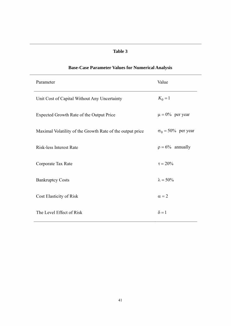
3. Numerical examples
We employ a numerical analysis by choosing the base-case parameter values as follow. A
firm expects that the output price will neither grow, nor decline, 0=μ . It can choose a
project such that the volatility of the output price is, at most, 50% per year, 0 50%σ = .13
The firm must pay an investment cost equal to one if the project is riskless, 0 1K = . All
agents face a riskless rate equal to 6% per year, i.e., 6%ρ = . The firm’s profits will be
taxed at 20%, i.e., 20%τ = .14 When the firm runs into bankruptcy, half of the firm value
will be lost, i.e., 0.5λ = . Finally, the cost elasticity of risk is 2.0α = and the level effect
of risk is 1δ = .
------------------------------------------------------------------------------------------------------------
Insert Table 3 here
------------------------------------------------------------------------------------------------------------
Table 4 reports the comparative statics results, with all values evaluated in line with
the optimal policies for the first-best firm, i.e., *fP P= , *
fθ = θ , and *fb b= . Given the
benchmark values given above, Panel A of Table 4 shows that if the current output price is
smaller than 0.1364, the level of the investment trigger *fP , then the first-best firm will
13 Pindyck (1988) indicates that, for most commodities, 50% is a plausible upper limit for the volatility of
the prices per year. 14 The tax rate τ is chosen to reflect that personal tax advantages to equity returns will lower the tax
advantage of debt below the corporate rate of 35 % (Leland, 1998).

26
wait until this critical level is reached; otherwise, the firm will invest immediately. At that
instant, the firm will choose a risk level equal to 9.71% per year ( * 0.1941fθ = ) and will
issue bonds that promise to pay $0.1356 per year, forever ( * 0.1356fb = ). After that instant,
the firm’s equity holders will not declare bankruptcy until the output price declines to the
level of the bankruptcy trigger, 0.1026 ( * 0.1026fP = ). At the instant of exercising the
investment option, the firm’s debt value, dfV , will be equal to $1.610, and its equity value,
efV , will be equal to $0.636. Thus, the optimal leverage ratio, /d
f f fL V V= , will be equal
to 71.7%, the yield spread, fR −ρ , will be equal to 242 bps (basis points), and firm’s net
value, ,fV K− will be equal to 1.241.
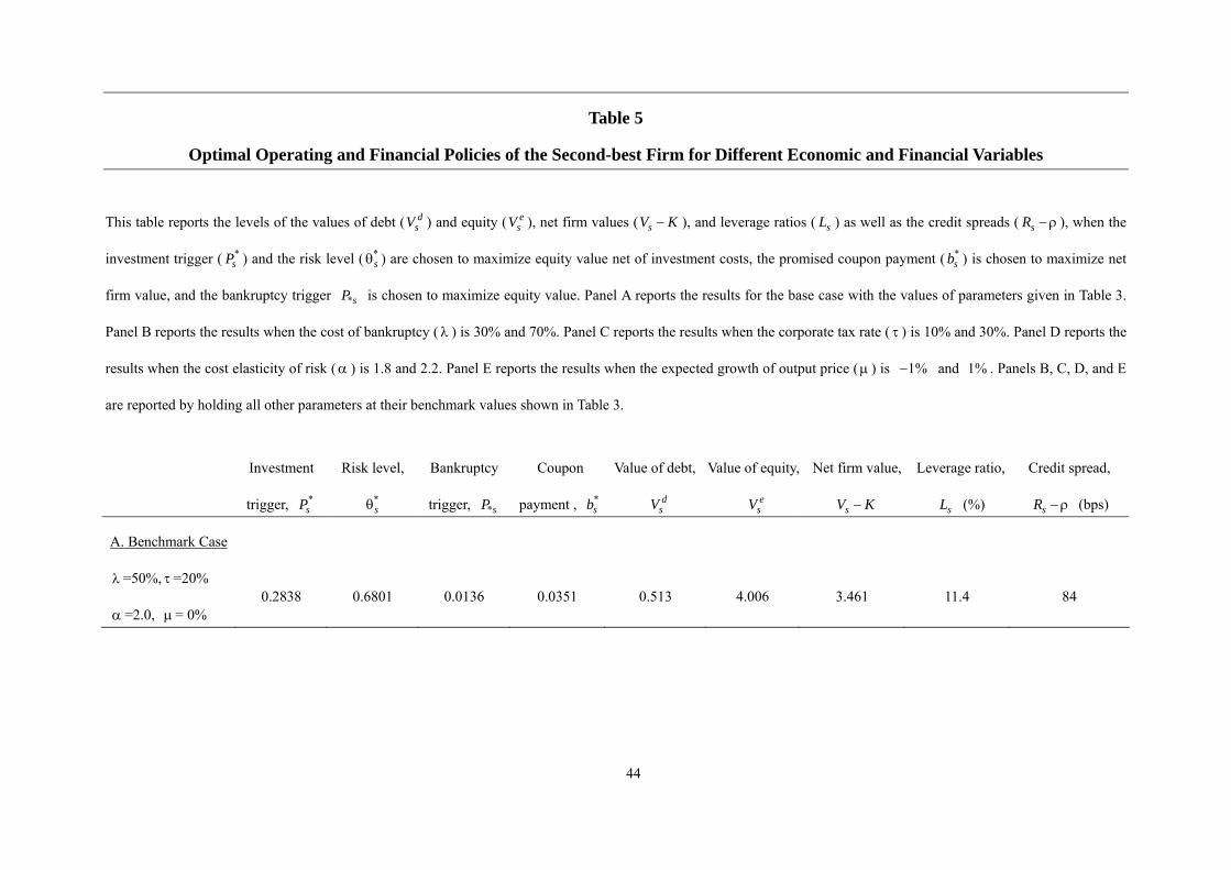
The results of our simulation analysis, presented in Table 5, satisfy the requirements
that debt overhang will arise, i.e., * / 0sP b∂ ∂ > , and that asset substitution will arise, i.e.,
* / 0s b∂θ ∂ > . These results help us explain the reason for the results shown in Tables 4 and
5. Table 5 reports the comparative statics results, where all values are evaluated at the
optimal policies for the second-best firm, i.e., *sP P= , *
sθ = θ , and *sb b= . Given the
benchmark values, Panel A of Table 5 shows that the values of the endogenous variables
for the second-best firm are as follow: The investment trigger *sP = 0.2838, which is 2.08
times its counterpart for the first-best firm, *fP ; the risk level of investment * 0.6801sθ = ,
which is 3.50 times *fθ ; the bankruptcy trigger * 0.0136sP = , which is 13.3% of * fP ; the
coupon payment * 0.0351sb = , which is 25.8% of *fb ; the debt value 0.513d
sV = , which

27
is 31.8% of dfV ; the equity value 4.006e
sV = , which is 6.29 times efV ; the credit spread
of corporate debt 84sR −ρ = bps, which is 34.7% of fR −ρ ; the net firm value
3.461sV K− = , which is 2.79 times fV K− ; and the leverage ratio 11.4%sL = , which is
15.9% of fL .
In other words, as compared to the first-best firm that is concerned with the joint
welfare of equity and debt holders, the second-best firm, which is concerned only with
equity holders after debt is in place, will delay investment and choose a higher risk level.
The second-best firm, which bears more risk and issues fewer bonds than the first-best firm,
benefits equity holders, but harms debt holders. As a result, the leverage ratio will be lower
for the second-best firm than for the first-best firm. Given that the second-best firm’s
creditors will anticipate the future behavior of the firm’s equity holders, they will thus
require fewer premiums on corporate debt than the first-best firm’s creditors.
We can investigate the optimal operating and financial policies for both the first- and
second-best firms to explain how they differ in these strategies. Suppose that we evaluate
Equation (23) at *sP P= , *
sb b= , and *sθ = θ . We find that:
2* *
* * * * * * 2
* 1( , , ) ( , , ) [( ) (1 ) 1] 0,e s s
s s s s s ss
b PW P b W P bP
β βθ = θ + − − <
ρ β (34)
where * * *( , , ) 0es s sW P b θ = in Equation (34) and * / 0sP b∂ ∂ > . Equation (34) thus indicates
that, from the viewpoint of debt holders, a firm that exercises the investment option at the

28
second-best trigger is too late, because the option value attributed to debt holders is
outweighed by what debt holders can get from investing immediately. That is, debt holders
will gain if the firm exercises the investment option at the first-best trigger.
Supposing that we evaluate Equation (18) at *sP P= , *
sb b= , and *sθ = θ . We find
that:
2
* * * * * *
* * *0 2
22 * *
( ( , , ) ) ( ( , , ) )
( ) [1 (1 )(1 ) ln ( (1 (1 )(1 )) 1] 0,(1 )
es s s s s s
s s s
s s
V P b K V P b K
b P PP P
β
∂ θ − ∂ θ −=
∂θ ∂θ
σ ∂β+ − −λ − τ + β − −λ − τ − <ρ −β ∂σ
(35)
where * * *( ( , , ) ) / 0es s sV P b K∂ θ − ∂θ = in Equation (35) and * / 0s b∂θ ∂ > .15 Equation (35)
indicates that, from the viewpoint of debt holders, a firm that chooses the second-best risk
strategy is too risky. That is, debt holders will gain if the firm chooses the first-best risk
strategy that involves a lower risk on investment.
After debt is in place, a firm that takes on more debt affects firm value through two
channels. First, the firm invests too late, which raises firm value as the firm exercises the
investment option at a better state, i.e., the second term on the right-hand side of Equation
(33) is positive. Second, the firm bears overly high risks, which reduces firm value, i.e., the
last term on the right-hand side of Equation (33) is negative. We find that the former effect
dominates the latter one. As a result, in Equation (33) the first term on the right-hand side
15 Given that * / 0s b∂θ ∂ > , the second-term on the right-hand side of Equation (35) will be negative if 1 1
2/( ) [1 ( (1 (1 )(1 )) ]− −ρ ρ −μ > − β − − λ − τ , which holds for the parameter values we use in the simulation.
29
is negative, i.e., * * *( ( , , ) ) / 0s s sV P b K b∂ θ − ∂ < . This suggests that, from the viewpoint of
debt holders, a firm that chooses the second-best debt financing strategy issues too many
bonds. That is, debt holders will prefer the firm to take on less debt.
------------------------------------------------------------------------------------------------------------
Insert Table 3 here
------------------------------------------------------------------------------------------------------------
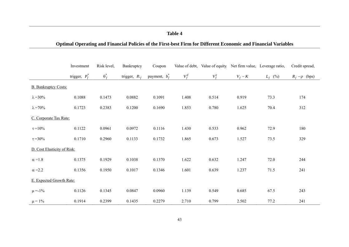
Panels B through E of Table 4 report the effects of bankruptcy costs (λ=0.3, or 0.7),
corporate taxes ( τ=10%, or 30%), the cost elasticity of risk ( 1.8 or 2.2α = ), and the
expected growth rate of the output price ( 1%μ = − , or 1%), on the firm’s policy choices
and values. Note that all the other parameters are held at their benchmark values.
Panel B of Table 4 gives the optimal operating and financial policies for bankruptcy
costs, λ , of 30% and 70%. Column 5 in Table 2 indicates that given debt financing and
risk choices, the first-best firm will be more cautious on its investment timing choice when
it expects to incur larger bankruptcy costs. This effect still dominates the following effect:
The first-best firm that suffers more bankruptcy costs will issue fewer bonds (as shown in
Column 5 in Table 2) and will, thus, invest earlier due to the debt overhang effect. On the
other hand, as bankruptcy costs increase, the first-best firm will issue more bonds because
the following dominating effect: The first-best firm will invest later and, at this better state,

30
will take on more debt. Given that the firm issues more bonds, it will be more prone to
bankruptcy. Finally, the first-best firm which incurs more bankruptcy costs will choose a
more risky project, because it invests at a better state and is, therefore, willing to bear more
risks. The optimal leverage ratio also decreases as λ increases.16 Surprisingly, all the
debt value, equity value, and the firm’s net value increase when bankruptcy costs are
increased. This is perhaps due to the fact that the output price at which a firm decides to
invest is more favorable when bankruptcy costs are larger. We also find that the credit
spread of risky debt increases as λ increases. The reason is as follows. An increase in λ
has two effects: First, debt value will decrease, which increases the credit spread; second,
the optimal operating and financial policies will be affected, and the credit spread may,
therefore, decrease. In our specific example, the net effect is positive because the first
effect always dominates the second one. This finding contrasts with the results of Leland
(1994) and Mauer and Ott (2000), who find that the net effect is negative.
As bankruptcy costs increase, Panel B of Table 5 shows that the second-best firm
actually issues more bonds. This is due to the following reason. As λ increases, the
marginal bankruptcy costs of debt financing increase, which reduces debt financing.
Nevertheless, this is dominated by the following effect: The firm’s value will increase as
16 Our result differs from that of Fries et al. (1997). They show that, given a firm’s residual value is equal to
zero at closure, i.e., λ =1 in our case, a firm in a competitive industry equilibrium will issue no bonds at all. Note that their result is based upon the assumptions that the number of firms is endogenously determined and that firms can freely enter and exit the output market.

31
the firm issues more bonds because the firm then exercises the investment option at a
better state. This beneficial effect is more significant as λ increases. Given that the firm
will issue more bonds as λ increases, the firm will invest later as a result of the debt
overhang effect, and take more risks as a result of the asset substitution effect. The firm
will also declare bankruptcy earlier, given that it takes on more debt. Larger bankruptcy
costs harm debt holders, but benefit equity holders. As a result, net firm value increases,
the leverage ratio decreases, and debt holders require a large premium when purchasing
corporate bonds.
Panel C of Table 4 reports the optimal operating and financial policies for the
corporate tax rates of 10% and 30%. Column 6 in Table 2 indicates that, given financing
and risk choices, the first-best firm will delay investment as the corporate tax rate increases.
As the corporate tax rate increases, the firm will receive more tax shielding and will,
therefore, issue more bonds. This will delay investment, as indicated in Column 2 of Table
2. Similarly, as the corporate tax rate increases, the following effect will reinforce the
effect resulting from the tax shield benefit: The firm will invest at a better state and will,
therefore, issue more bonds. Given that the firm issues more bonds, the firm will also
declare bankruptcy earlier. As the corporate tax rate increases, the first-best firm will also
bear more risks, because the following effect dominates: The firm invests at a better state
and will, therefore, take on more risks. As the corporate tax rate increases, the first-best

32
firm’s equity value is also significantly increased, such that the leverage ratio is decreased.
Finally, as the corporate tax rate increases, the credit spread will increase, as bondholders
expect bankruptcy costs to be increasingly imminent.
Panel C of Table 5 indicates that, as the corporate tax rate increases, the second-best
firm will invest later, issue more bonds, and take on more risks. Column 6 of Table 2
indicates that, given debt financing and risk choices, the second-best firm will invest later
as the corporate tax rate increases. This effect seems to dominate all the other effects. As
the firm invests at a better state, the firm will, therefore, issue more bonds and bear more
risks. Given that the firm issues more bonds, the firm will also declare bankruptcy earlier.
As the corporate tax rate increases, the second-best firm will have higher debt value since
more bonds are issued and lower equity value. As a result, net firm value will increase
because debt value is increased more than the reduction in equity value. Furthermore, the
leverage ratio, as well as the credit spread of debt, will also increase.
Panel D of Table 4 reports the optimal operating and financial policies for the
first-best firm for two different levels of cost elasticity of risk, 1.8α = and 2.2. In
Column 7 of Table 2, an increase in the cost elasticity of risk will induce the first-best firm
to invest earlier, holding all the other decisions as given. This effect still dominates all the
other effects. Given that the firm invests earlier, the firm will, therefore, issue fewer bonds
and delay declaring bankruptcy. The firm may take on less risky projects, as it invests

33
earlier. This is, however, dominated by the following effect: Column 7 of Table 2 indicates
that, given investment timing and financing decisions, the first-best firm will bear more
risk as its cost elasticity of risk becomes higher. The value to debt holders will decrease,
given that the firm issues fewer bonds, but the value to equity holders will increase, given
that the firm chooses a higher risk level. As a result, the leverage ratio is decreased, and the
net firm value and the credit spread are both decreased.
Panel D of Table 5 indicates that the second-best firm will invest earlier, issue fewer
bonds, and bear less risk as the cost elasticity of risk increases. The reason for the
investment timing and debt financing resembles its counterpart for the first-best firm. The
reason for its bearing less risk is as follows. As indicated by Column 7 of Table 2, as the
cost elasticity of risk increases, the second-best firm will bear more risk. This effect is,
however, dominated by the effect, as follows: The firm will invest earlier and, thus, bear
less risk. Furthermore, given that the firm issues fewer bonds, it will also declare
bankruptcy later. As a result of an increase in the cost elasticity of risk, the second-best
firm will have lower debt and equity values and, therefore, lower net firm value. The
leverage and credit spread will also decrease as a result.
Panel E of Table 4 shows that, except for the leverage ratio and the credit spread of
debt, the effects of an increase in the expected growth rate of the output price (μ ) on all the
other endogenous variables of the first-best firm parallel those of an increase in the

34
corporate tax rate. The leverage ratio will increase as debt holders gain more than equity
holders from an increase in the growth rate of the output price. Consistent with the finding
presented in Column 7 of Table 1, an increase in the expected growth rate of the output
price reduces the credit spread of risk debt.
Panel E of Table 5 shows that the comparative statics results of μ on endogenous
variables of the second-best firm resemble those of the first-best firm, with the exception
of those for *sP and /dsV V . That is, an increase in the expected growth rate of the output
price discourages the second-best firm to declare bankruptcy and to reduce its choice of the
leverage ratio.
------------------------------------------------------------------------------------------------------------
Insert Tables 4, 5 here
------------------------------------------------------------------------------------------------------------
The net value of the second-best firm is higher than the net value of the first-best firm
when both are evaluated by their respective optimal exercise timing. Given that the
first-best firm invests earlier than the second-best firm, we should compare their respective
firm values at the investment option exercise timing for the first-best firm *fP . The
second-best firm, therefore, has an option value equal to
1* * * * * *0 0( / ) ( ( , , ) (1 ) )f s s s s sP P V P b Kβ α αθ − + δθ σ , as compared to the net firm value of the
35
first-best firm, which is given by * * * *0 0( , , ) (1 ) )f f f fV P b Kα αθ − + δθ σ . Table 6 indicates that,
given the benchmark parameter values, when the output price reaches the critical level that
justifies the first-best firm to exercise the investment option, *fP , the probability that the
second-best firm will exercise the investment option is only 30.1%. Multiplying this
probability with the net value of the second-best firm yields the expected net value for the
second-best firm, at *fP P= , which is lower than the net value for the first-best firm by a
magnitude of 0.197, or by 15.8% of the first-best firm’s value. This is significantly higher
than the value obtained from Leland (1998) and Mauer and Sarkar (2005), as we consider
two types of agency costs, rather than one single type of agency cost. We also find that the
(percentage) agency cost is larger when the bankruptcy cost is lower, the corporate tax rate
is lower, and the cost elasticity of risk is lower.
------------------------------------------------------------------------------------------------------------
Insert Tables 6 here
------------------------------------------------------------------------------------------------------------
4. Conclusions
This article has compared the debt financing, investment timing, risk, and bankruptcy
decisions of the second-best firm and the first-best firm; The former incurs agency costs of
the kinds conjectured by Jensen and Meckling (1976) and Myers (1977), and the latter is

36
able to avoid these agency costs. We find that, after debt is in place, an increase in debt
induces the second-best firm to delay investment and choose an overly risky level. As a
result, as compared to the first-best firm, the second-best firm will invest later, bear more
risks, and issue more bonds. We also find that the agency cost of debt is about 15.8% of the
first-best firm’s value, due to the suboptimal operating and financial policies of the
second-best firm.
This article builds a simplified model and, thus, can be extended in the following way.
First, this article may allow renegotiation between equity and debt holders (Sundaresan and
Wang, 2007). Second, this article may allow strategic interactions between firms (Jou and
Lee, 2008; Novy-Marx, 2007; Zhdanov, 2007). Finally, this article may allow a firm to
choose the maturity of debt (Goldstein, Ju and Leland, 2001), or bank loans (Hackbarth,
Hennessy and Leland, 2007).
References
Black, F., and J. Cox. 1976. Valuing Corporate Securities: Some Effects of Bond Indenture Provisions. Journal of Finance, 31: 351-367.
Brennan, M. J., and E. S. Schwartz. 1984. Valuation of Corporate Claims. Journal of Finance, 39: 593-607.
Dixit, A. K. 1993. Choosing Among Alternative Discrete Investment Projects under Uncertainty. Economics Letters, 41: 265-268.
Dixit, A. K., and R. S. Pindyck. 1994. Investment under Uncertainty, New Jersey:
37
Princeton University Press.
Ericsson, J. 2000. Asset Substitution, Debt Pricing, Optimal Leverage and Maturity. Finance, 21: 39–70.
Fries, S., M. Miller, and W. Perraudin. 1997. Debt in Industry Equilibrium. Review of Financial Studies, 10: 39-67.
Gavish, B., and A. Kalay. 1983. On the Asset Substituion Problem. Journal of Financial and Quantitative Analysis, 18: 21-31.
Green, R., and E. Talmor. 1986. Asset Substitution and the Agency Costs of Debt Financing. Journal of Banking and Finance, 10: 391-399.
Goldstein, R. S., N. Ju, and H. E. Leland. 2001. An EBIT-based Model of Dynamic Capital Structure. Journal of Business, 74: 483-512.
Hackbarth, D., C. A. Hennessy, and Leland, H. E. 2007. Can the Trade-off Theory Explain Debt Structure? Review of Financial Studies, 20(5): 1389-1428.
Jensen, M. C., and W. H. Meckling. 1976. Theory of the Firm: Managerial Behavior, Agency Costs, and Capital Structure. Journal of Financial Economics, 4: 177-203.
Jou, J-B., and T. Lee. 2004. The Agency Problem, Investment Decision and Optimal Financial Structure. European Journal of Finance, 10: 489–509.
Jou, J-B., and T. Lee. 2008. Irreversible Investment, Financing, and Bankruptcy Decisions in and Oligopoly. Journal of Financial and Quantitative Analysis, 43: 769-786.
Leland, H. E. 1994. Corporate Debt Value, Bond Covenants, and Optimal Capital Structure. Journal of Finance, 49: 1213-1252.
Leland, H. E. 1998. Agency Costs, Risk Management, and Capital Structure. Journal of Finance, 53: 1213-1244.
Mao, C. X. 2003. Interaction of Debt Agency Problems and Optimal Capital Structure: Theory and Evidence. Journal of Financial and Quantitative Analysis, 38(2): 399-423.
Mauer, D. C., and S. H. Ott. 2000. Agency Costs, Investment Policy and Optimal Capital Structure: The Effect of Growth Options, in Project Flexibility, Agency and Market Competition: New Developments in the Theory and Application of Real Options, 151-179. London: Oxford University Press.
Mauer, D. C., and S. Sarkar. 2005. Real Options, Agency Conflicts, and Optimal Capital Structure. Journal of Banking and Finance, 29: 1405–1428.
38
Mello, A. S., and J. E. Parsons. 1992. The Agency Costs of Debt. Journal of Finance, 47: 1887-1904.
Mello, A. S., J. E. Parsons, and A. J. Triantis. 1995. An Integrated Model of Multinational Flexibility and Financial Hedging. Journal of International Business, 39: 27-51.
Myers, S. 1977. Determinants of Corporate Borrowing. Journal of Financial Economics, 5: 147-175.
NCREIF report, 2008. The National Council of Real Estate Investment Fiduciaries, Washington, D. C.
Novy-Marx, R. 2007. An Equilibrium Model of Investment Under Uncertainty. Review of Financial Studies, 20(5): 1461-1502.
Pindyck, R. 1988. Irreversible Investment, Capacity Choice, and the Value of the Firm. American Economic Review, 79(6): 969-985.
Sundaresan, S., and Wang, N. 2007. Investment under Uncertainty with Strategic Debt Service. American Economic Review, 97(2): 256-261.
Vanden, J. M. Asset Substitution and Structured Financing, forthcoming in the Journal of Financial and Quantitative Analysis.
Zhdanov, A. 2007. Optimal Capital Structure in a Duopoly. Journal of Financial and Quantitative Analysis, 42: 709-734.

39
Table 1
Comparative Statics of Financial Variables
This table describes properties of the equations for debt value, dV , the value of equity, eV , the total firm value, V , and the yield spread of
the risky debt over the risk-free rate, R −ρ . The term P is the output price, *P is the bankruptcy trigger, b is the coupon paid on debt,
σ and μ are, respectively, the instantaneous volatility and the expected growth of /dP P , λ is the fraction of asset value lost if
bankruptcy occurs, τ is the corporate tax rate, α is the cost elasticity of risk, and ρ is the risk-free interest rate of demand.
Limit as Sign of Change in Instrument for an Increase in:
Variable Shape P →∞ *P P→ b σ λ μ τ α P
dV
Concave
in P , b
bρ
(1 )(1 )( )
P−λ − τ
ρ −μ
>0;
<0 as *P P→
<0;
>0 as *P P→
<0 >0 <0 0 >0
eV
Convex in
P , b
(1 )( )P b− τ −
ρ−μ ρ0 <0 >0 0
<> 0 <0 0 >0
V
Concave
in P , b
(1 )( )
P b− τ τ+
ρ−μ ρ (1 )(1 )
( )P
−λ − τρ −μ
>0;
<0 as *P P→
<0;
>0 as *P P→
<0 <> 0 <0 0 >0
R −ρ
Convex in
P , b
0
12
2
(1 )(1 )[1 ( 1)]
( 1)−−α − τ β
+ −β −
>0
>0;
<0 as *P P→
>0 <0 >0 0 <0

40
Table 2
Comparative Statics of a Financial or Operating Choice Variable, Holding the
Other Variables Constant
This table describes the properties of choices of the investment trigger, *fP , the bankruptcy trigger, * fP , the
risk level of investment, *fθ , and the coupon level, *
fb , for the first-best firm, and choices of the investment
trigger, *sP , and the risk of investment, *
sθ , for the second-best firm, when the other choices are held
constant. The term b is the coupon level, σ and μ are, respectively, the instantaneous volatility and
expected growth rate of /dP P , λ is the fraction of asset value lost if bankruptcy occurs, τ is the
corporate tax rate, α is the cost elasticity of risk, and P is the output price.
Signs of change in variable for an increase in:
Variable b σ μ λ τ α P
*fP >0
<> 0
<> 0 >0 >0 *0< N.A.
* fP >0 <0 <0 0 0 0 N.A.
*fθ
<> 0 N.A.
<> 0 >0
<> 0 **0>
<> 0
*fb N.A.
<> 0
<> 0 <0 >0 0 >0
*sP
<> 0
<> 0
<> 0 0 >0 *0< N.A.
*sθ
<> 0 N.A.
<> 0 0 <0 **0>
<> 0
Notes: N.A. refers to not available; * holds for 1σ < , ** holds for 1/e− ασ < . That is, the sign holds when
60.7%σ < for 2α = (the benchmark case in simulation analysis).
41
Table 3
Base-Case Parameter Values for Numerical Analysis
Parameter Value
Unit Cost of Capital Without Any Uncertainty 0 1K =
Expected Growth Rate of the Output Price 0%μ = per year
Maximal Volatility of the Growth Rate of the output price 0 50%σ = per year
Risk-less Interest Rate 6%ρ = annually
Corporate Tax Rate 20%τ =
Bankruptcy Costs 50%λ =
Cost Elasticity of Risk 2α =
The Level Effect of Risk 1δ =

42
Table 4
Optimal Operating and Financial Policies of the First-best Firm for Different Economic and Financial Variables
This table reports the levels of the values of debt ( dfV ), equity ( e
fV ), net firm values ( fV K− ), and leverage ratios ( fL ), as well as the credit spreads ( fR −ρ ), when the
investment trigger ( *fP ), promised coupon payment ( *
fb ), and risk level ( *fθ ) are all chosen to maximize net firm values, and the bankruptcy trigger ( * fP ) is chosen to
maximize equity value. Panel A reports the results for the base case with the values of parameters given in Table 3. Panel B reports the results when the cost of bankruptcy ( λ )
is 30% and 70%. Panel C reports the results when the corporate tax rate ( τ ) is 10% and 30%. Panel D reports the results the cost elasticity of risk (α ) is 1.8 and 2.2. Panel E
reports the results when the expected growth of output price (μ ) is 1%− and 1% . Panels B, C, D, and E are reported by holding all other parameters at their benchmark
values shown in Table 3.
Investment
trigger, *fP
Risk level,
*fθ
Bankruptcy
trigger, * fP
Coupon
payment, *fb
Value of debt,
dfV
Value of equity,
efV
Net firm value,
fV K−
Leverage ratio,
fL (%)
Credit spread,
fR −ρ (bps)
A. Benchmark Case
λ =50%, τ =20%
α =2.0, μ = 0% 0.1364 0.1941 0.1026 0.1356 1.610 0.636 1.241 71.7 242
43
Table 4
Optimal Operating and Financial Policies of the First-best Firm for Different Economic and Financial Variables
Investment
trigger, *fP
Risk level,
*fθ
Bankruptcy
trigger, * fP
Coupon
payment, *fb
Value of debt,
dfV
Value of equity,
efV
Net firm value,
fV K−
Leverage ratio,
fL (%)
Credit spread,
fR −ρ (bps)
B. Bankruptcy Costs:
λ =30%
λ =70%
0.1088
0.1723
0.1473
0.2383
0.0882
0.1200
0.1091
0.1690
1.408
1.853
0.514
0.780
0.919
1.625
73.3
70.4
174
312
C. Corporate Tax Rate:
τ =10%
τ =30%
0.1122
0.1710
0.0961
0.2960
0.0972
0.1133
0.1116
0.1732
1.430
1.865
0.533
0.673
0.962
1.527
72.9
73.5
180
329
D. Cost Elasticity of Risk:
α =1.8
α =2.2
0.1375
0.1356
0.1929
0.1950
0.1038
0.1017
0.1370
0.1346
1.622
1.601
0.632
0.639
1.247
1.237
72.0
71.5
244
241
E. Expected Growth Rate:
μ =-1%
μ = 1%
0.1126
0.1914
0.1345
0.2399
0.0847
0.1435
0.0960
0.2279
1.139
2.710
0.549
0.799
0.685
2.502
67.5
77.2
243
241
44
Table 5
Optimal Operating and Financial Policies of the Second-best Firm for Different Economic and Financial Variables
This table reports the levels of the values of debt ( dsV ) and equity ( e
sV ), net firm values ( sV K− ), and leverage ratios ( sL ) as well as the credit spreads ( sR −ρ ), when the
investment trigger ( *sP ) and the risk level ( *
sθ ) are chosen to maximize equity value net of investment costs, the promised coupon payment ( *sb ) is chosen to maximize net
firm value, and the bankruptcy trigger *sP is chosen to maximize equity value. Panel A reports the results for the base case with the values of parameters given in Table 3.
Panel B reports the results when the cost of bankruptcy ( λ ) is 30% and 70%. Panel C reports the results when the corporate tax rate ( τ ) is 10% and 30%. Panel D reports the
results when the cost elasticity of risk (α ) is 1.8 and 2.2. Panel E reports the results when the expected growth of output price (μ ) is 1%− and 1% . Panels B, C, D, and E
are reported by holding all other parameters at their benchmark values shown in Table 3.
Investment
trigger, *sP
Risk level,
*sθ
Bankruptcy
trigger, *sP
Coupon
payment , *sb
Value of debt,
dsV
Value of equity,
esV
Net firm value,
sV K−
Leverage ratio,
sL (%)
Credit spread,
sR −ρ (bps)
A. Benchmark Case
λ =50%, τ =20%
α =2.0, μ = 0% 0.2838 0.6801 0.0136 0.0351 0.513 4.006 3.461 11.4 84

45
Table 5
Optimal Operating and Financial Policies of the Second-best Firm for Different Economic and Financial Variables
Investment
trigger, *sP
Risk level,
*sθ
Bankruptcy
trigger, *sP
Coupon
payment , *sb
Value of debt,
dsV
Value of equity,
esV
Net firm value,
sV K−
Leverage ratio,
sL (%)
Credit spread,
sR −ρ (bps)
B. Bankruptcy Costs:
λ =30%
λ =70%
0.2829
0.2854
0.6781
0.6828
0.0135
0.0137
0.0350
0.0353
0.518
0.510
3.995
4.024
3.456
3.475
11.5
11.3
77
92
C. Corporate Tax Rate:
τ =10%
τ =30%
0.2505
0.3253
0.6762
0.6828
0.0121
0.0155
0.0310
0.0400
0.455
0.582
4.055
3.943
3.453
3.467
10.1
12.9
81
87
D. Cost Elasticity of Risk:
α =1.8
α =2.2
0.3242
0.2603
0.7350
0.6400
0.0142
0.0127
0.0392
0.0310
0.559
0.463
4.490
3.748
3.966
3.170
11.4
11.0
102
69
E. Expected Growth Rate:
μ =-1%
μ = 1%
0.2613
0.3018
0.6046
0.7462
0.0152
0.0114
0.0320
0.0367
0.471
0.537
3.239
5.038
2.664
4.506
12.7
9.6
81
83

46
Table 6
The Agency Cost of Debt
(1)
Net value of the
first-best firm,
fV K− ($)
(2)
Net value of the
second-best firm,
sV K− ($)
(3)
Probability of Exercising,
1* *( / )f sP P β (%)
(4)=(1)–(2)*(3)
Agency Cost of Debt
($)
(5)=(4)/(1)
Percentage of Agency Cost
(%)
A. Benchmark Case
λ =50%, τ =20%
α =2.0, μ = 0% 1.241 3.461 30.2 0.196 15.8
B. Bankruptcy Costs:
λ =30%
λ =70%
0.919
1.625
3.456
3.475
21.0
43.9
0.196
0.112
21.3
6.9
C. Corporate Tax Rate:
τ =10%
τ =30%
0.962
1.527
3.453
3.467
26.9
35.0
0.033
0.315
3.4
20.6

47
Table 6
The Agency Cost of Debt
(1)
Net value of the
first-best firm,
fV K− ($)
(2)
Net value of the
second-best firm,
sV K− ($)
(3)
Probability of Exercising,
1* *( / )f sP P β (%)
(4)=(1)–(2)*(3)
Agency Cost of Debt
($)
(5)=(4)/(1)
Percentage of Agency Cost
(%)
D. Cost Elasticity of Risk:
α =1.8
α =2.2
1.247
1.237
3.966
3.170
24.6
34.4
0.271
0.145
21.7
11.7
E. Expected Growth Rate:
μ =-1%
μ = 1%
0.685
2.502
2.664
4.506
20.1
51.6
0.150
0.174
21.9
4.0