* I would like to thank Erik Hurst, Jiro Kondo and David Matsa for helpful comments. I would also like

to thank Laura Paszkiewicz from the BLS for help with the Consumer Expenditure data. Data was

warehoused by ICPSR. Aaron Yoon and Kexin Qiao provided helpful research assistance.

Mortgage Debt Overhang:

Reduced Investment by Homeowners with Negative Equity

Brian T. Melzer*

August 2010

[Do not cite without author’s permission]

Abstract

Homeowners with negative equity have less incentive to invest in their property. They

face a debt overhang: in expectation, some value created by equity investments in the property

will go to the lender. Using rich microdata on household expenditures, I show that debt overhang

plays an important role in household financial decisions. I find that homeowners with negative

equity cut back substantially on mortgage principal payments, home improvements and home

maintenance spending. At the same time, these households show no difference in durable

spending on automobiles, furniture and home appliances, investments that are not attached to the

home. The decline in mortgage principal payments is particularly large for negative equity

homeowners in non-recourse states, where strategic default is more likely because lenders have

limited claim on non-housing wealth. Debt overhang, rather than financial constraints, best

explains this set of facts. Given the prevalence of negative home equity in today’s housing

market, the results suggest that home prices will grow more slowly in the future because of

underinvestment. In addition, the potential deadweight loss due to home foreclosures is only part

of the economic inefficiency that follows the spree of mortgage borrowing in the 2000s and the

subsequent real estate price decline.

2

I. Introduction

A long-standing and important idea in finance theory is that leverage can distort

investment decisions. Myers (1977) introduces the notion of corporate debt overhang,

emphasizing that high leverage can cause firms to underinvest, since the benefits of new capital

investments accrue largely to debt holders rather than equity holders. In public finance, Keynes

(1920), Krugman (1988) and Sachs (1990) emphasize that heavy public debt loads reduce

incentives for public sector investments in infrastructure and private sector investments in

physical and human capital. This paper applies the same thinking to household financial

decisions, and provides evidence that households with mortgage debt overhang underinvest in

their homes.

The reasoning behind debt overhang is straightforward. For an incremental investment in

a debt-free asset, the owner captures the investment’s payoffs in all states of the world. In

contrast, for a levered asset with some risk of default, the investment’s payoffs accrue to the

foreclosing lender if the owner defaults. Faced with the same investment outlay today and the

prospect of sharing the future payoffs with the lender, the owner of a levered asset may

underinvest, foregoing some investments that have positive net present value for a debt-free

owner.

Following the precipitous decline in the United States housing market between 2007 and

2009, during which average home prices fell by 14% nationwide and by as much as 50% in some

states1, mortgage debt overhang has become an important issue. Up to 20% of homeowners are

in a negative equity position, facing mortgage liabilities that exceed the value of their home.

1 These figures are based on Fiserv Case-Shiller Home Price Index data between the second quarter of 2007 and the

first quarter of 2009. State-level declines of 40 to 50% occurred in AZ, CA, FL, MI and NV.

3

Understanding how these homeowners behave is important in forecasting home prices, mortgage

defaults and residential investment, and in evaluating foreclosure reduction policies.

This paper contributes to these broad goals by answering, first, whether housing

investments, in the form of improvements, maintenance and mortgage principal payments, differ

among negative equity households and, second, whether debt overhang explains these

differences. To answer these questions, I use rich household microdata from the Bureau of Labor

Statistics’ Consumer Expenditure Survey (CE). These data contain comprehensive property-

specific information for a national sample of homeowners, including mortgage balances and

principal payments, home improvement and maintenance expenditures, and property values as

estimated by the homeowners. I construct an estimate of mortgage loan-to-value and an indicator

for negative home equity, and use regression analysis to estimate the difference in housing

investment between homeowners with and without large mortgage debts.

I find that negative equity homeowners invest $215 less in home improvements and

maintenance on average, a 30% reduction relative to positive equity homeowners. Households

with negative equity also pay $370, or 25%, less in mortgage principal, controlling for

differences in mortgage balance. This disparity in home investment is not explained by

differences in total expenditures, income or wealth. Nor is it explained by variation in household

demographic characteristics like age, race, education and household size, or property

characteristics like property value, age of home, duration of ownership and various traits of the

physical structure.

The detailed, household-level data of the CE are useful in narrowing the interpretation of

the empirical results and ruling out alternatives to the debt overhang interpretation. Aside from

indicating debt overhang, negative equity may proxy for other differences between households –

4

differences in wealth, borrowing capacity and investment opportunities, or varied exposure to

economic shocks – that explain their lower home investment spending. For example, in

aggregate data at the state or MSA level a negative correlation between mortgage loan-to-value

and home improvements might arise from regional economic shocks that reduce real estate

values, wealth, employment and household spending, including spending on home-related

investments. However, this mechanism does not explain my findings, which are identified using

household-level variation in negative equity, conditional on total expenditures. Borrowing and

liquidity constraints also fail to explain the results: among homeowners with higher income and

limited unsecured debt, who are evidently not financially constrained, negative equity still

predicts lower spending on home investments. Finally, it is natural to question whether negative

equity homeowners, many of whom have experienced a large decline in their home’s value,

invest less because they perceive low returns from improvements. Even debt-free owners might

invest less in these circumstances. But this line of thinking does not account for the reduction in

principal payments, which do not change the underlying asset and therefore should not fall

simply due to low forecast returns from marginal investments.

Two falsification exercises strengthen the case for debt overhang by confirming that

negative equity is unrelated to durable investments in categories that are not subject to mortgage

overhang. Notably, negative equity homeowners do not spend less on furniture and home

appliances, which are home improvements that face no overhang because they are not sacrificed

to the lender in the case of default. Nor do they cut spending on new and used vehicles. Viewed

together with the main results, this evidence strongly supports debt overhang relative to other

accounts, since it demonstrates within-household variation in overhang that explains the

investment patterns of negative equity homeowners. Alternative hypotheses that postulate a

5

household-level difference among heavily indebted homeowners – like the expectation of low

future income or the preference to invest little in home improvement and durables – would not

account for these facts.

The final extension of the main analysis tests whether the choices of negative equity

homeowners depend on state foreclosure laws. Ten states provide mortgage creditors with

recourse, or the ability to claim mortgage debtors’ other assets when the value of the collateral

falls short of the loan balance. If negative equity homeowners in these states are less likely to

default, as Ghent and Kudlyak (2009) find, they should also be less likely to cut back on

principal payments and home improvements. Evidence on this point is mixed. Negative equity

reduces principal payments more in non-recourse states, but has a similar effect on home

improvements in recourse and non-recourse states.

The motivation for this research is threefold. First, the impact of financial distress among

homeowners and the optimal policy response are important issues. This paper extends the

existing literature on negative equity – which focuses on negative equity’s role as a cause of

mortgage default (Foote, Gerardi and Willen 2008; Guiso, Sapienza and Zingales 2009; Bhutta,

Dokko and Shan 2010) and reduced household mobility (Chan 2001; Ferreira, Gyourko and

Tracy 2008) – to provide new evidence on how and why negative equity borrowers change their

behavior. Regarding foreclosure reduction policy, my findings highlight the importance of

mortgage principal reduction in restoring homeowners’ incentives to pay their mortgages,

consistent with Haughwout, Okah and Tracy (2009), but also to care for their homes. The latter

point suggests an additional economic motivation for principal reduction as part of mortgage

modification programs: aside from preventing foreclosure-related externalities, principal

6

reduction also mitigates underinvestment, encouraging the optimal level of residential housing

investment.2

Second, surprisingly little research examines the empirical relevance of debt overhang,

even though this friction is a common feature of theoretical models within corporate, public and

macro finance. In light of the recent housing crisis, Mulligan (2008) even proposes a model of

labor supply in which mortgage debt overhang plays a crucial role.3 But the only empirical study

on this topic is Olney (1999), who finds loan delinquency patterns during the great depression

that are consistent with debt overhang.4 I provide more direct and expansive evidence, grounded

in microdata, that households are forward looking in their investment choices and that household

balance sheet quality affects these choices above and beyond the effect of liquidity constraints.5

Third, home improvement decisions are worthy of study in their own right. Mendelsohn

(1977) and Montgomery (1992) offer descriptive analyses of improvement spending across

households, and Gyourko and Tracy (2006) find a small role for improvement spending in

consumption smoothing. But more work is needed to understand the variety of economic factors

that influence these decisions. For households outside the top income decile, their home

constitutes roughly 50% of their total assets (Bucks et al. 2009), and home improvement

decisions are some of their most significant ongoing asset management decisions. The

contributions of home improvement and maintenance spending to the housing sector are also

sizeable. From 1993 to 2007 such spending averaged $142 billion (measured in 2009 dollars),

2 Campbell, Giglio and Pathak (forthcoming) examine foreclosure spillovers: they estimate a 1% reduction in home

price for each foreclosure with 0.05 miles. 3 In the model, heavily indebted homeowners work less to qualify for mortgage modifications that are available to

borrowers with low current income. 4 Households continued to pay installment loans secured by durable goods in which they typically had significant

equity, but ceased payments on (non-recourse) mortgages that likely exceeded their home’s value. 5 Hurst and Stafford (2006) find that home equity is used to finance current expenditures, particularly among those

that appear liquidity constrained. Mian and Sufi (forthcoming) observe that homeowners, particularly those that

seem to be liquidity constrained, borrow against increases in home equity and do not use the proceeds to pay down

other debt. The authors postulate that this borrowing finances consumption, including home improvement spending.

7

almost half of the $300 billion invested annually in construction of new homes over this period.

Annual maintenance and improvement spending, at 0.9% of the housing stock, is similarly large

relative to the long term growth in existing home values. Typical estimates call for real growth of

2-3% per year, so it is plausible that quality increases driven by improvement and maintenance

spending explain between one third and one half of this growth, especially considering that the

aggregate value of improvements and maintenance cited above exclude the value of

homeowners’ time.6 Viewed in this context, the empirical results of this paper suggest that home

prices will grow more slowly in the future, especially in states with substantial debt overhang.

The rest of the article proceeds as follows. The next section outlines the predictions tested

in the regression analysis. Section III describes the data and basic sample statistics. Sections IV

and V cover the regression model and estimation results. Section VI concludes.

II. Predictions: Debt Overhang, Negative Equity and Home-related Investments

This section outlines the testable predictions of the debt overhang hypothesis, with

discussion to highlight how these predictions differentiate debt overhang from other economic

mechanisms linking negative equity and housing investments. The empirical analysis that

follows uses an indicator for negative equity as a practical measure of debt overhang, so each

hypothesis is framed with negative equity status as the independent variable of interest. Section

III.2 provides further discussion of this choice.

6 The Historical Census of Housing Tables from the U.S. Census show 2.3% real growth in median home prices

from 1940 to 2000 (http://www.census.gov/hhes/www/housing/census/historic/values.html).

8

Prediction 1: Negative equity homeowners will invest less in improving and maintaining their

homes.

Studies of mortgage default show that default rates are substantially higher among

negative equity homeowners (Deng, Quigley and Van Order 2000; Deng and Gabriel 2006;

Foote, Gerardi and Willen 2008). Being closer to default, negative equity homeowners have less

incentive to improve the property, since doing so makes the debt claim more secure and valuable

without necessarily increasing the asset’s value to the owner.7 Stated otherwise, even a project

that achieves a certain return of $1.15 for every $1 invested looks unattractive if the lender keeps

the $1.15 payoff 10% of the time.

Prediction 2: Negative equity homeowners will reduce mortgage principal payments.

The reasoning behind Prediction 1 holds also for principal payments. When there is a

large debt overhang, principal payments are a poor investment because they pay off mostly to the

lender. Prediction 2 is useful in testing whether negative equity homeowners reduce home

improvement spending because they perceive limited home investment opportunities. Principal

payments should not be sensitive to this consideration. Their marginal return is determined by

the interest rate on the loan and the probability of default, and only indirectly by forecast returns

on the home or its renovation.8 So, for homeowners to cut back on principal payments they must

be responding to variation in the probability of default, i.e. variation in the extent of debt

overhang.

7 I assume that informational frictions – difficulty specifying optimal improvements and maintenance, and difficulty

identifying homeowners that are underinvesting – prevent borrowers and lenders from overcoming debt overhang

through ex ante contracting and contract renegotiation. 8 Forecast asset returns affect the likelihood of future default.

9

Prediction 3: The reduction in principal payments and home investments will not be limited to

negative equity homeowners that appear financially constrained.

Homeowners with negative equity might prefer to invest more in their home but are

unable to finance those expenditures. They lack a key source of secured funding – borrowing

against home equity through cash-out refinancing or a line of credit. In fact, homeowners that

refinance or take out home equity loans often report home improvement as the use of the

proceeds (Brady, Canner and Maki 2000), so accounting for liquidity constraints is crucial.

Prediction 3 separates debt overhang from financial constraints: debt overhang should

still affect the improvement spending of homeowners with higher income and limited unsecured

debt, who appear to have the borrowing capacity and liquidity to fund improvements.

Prediction 4 (Falsification): Negative equity homeowners will show no difference in spending on

durable investments that are not attached to the home, including outlays for vehicles and home

improvements that do not go to the mortgage lender, like furniture and home equipment.

Home improvements that are not part of the property’s physical structure, like furniture

and most home appliances, stay with the homeowner in the event of default. As do other durable

assets, like vehicles, provided that the mortgage lender lacks recourse or chooses not to exercise

this right. So the debt overhang hypothesis predicts no difference in expenditures on these items.

In contrast, other explanations that posit a different taste for durable or home-related spending

would predict lower spending in these categories too.

10

Prediction 5: The reduction in principal payments and home investments will be smaller for

negative equity homeowners in recourse states.

In states that provide mortgage lenders recourse to borrowers’ other assets or future

income, mortgage default among negative equity homeowners should be less likely. Particularly

for homeowners who are considering default because of a fall in home value rather than an event

like job loss or a shock to medical expenditures, the loss of other assets offsets the gain from

defaulting on the mortgage. Ghent and Kudlyak (2009) offer confirming evidence: default rates

among negative equity homeowners in recourse states appear to be at least 20 percent lower.

Accordingly, homeowners’ responses to debt overhang should be less dramatic in

recourse states. That is, the difference in principal payments and improvement spending

attributable to negative equity should be smaller in recourse versus non-recourse states.

III. Data

The primary data for this study come from the Consumer Expenditure Interview Survey,

which follows a rotating random sample of roughly 7,500 households for a year-long period and

provides quarterly observations on each household’s expenditures. These data are well-suited for

this study because they combine detailed information on housing expenditures with information

on mortgage debt and property characteristics, including the owner’s valuation of the home.

CE expenditure data are extraordinarily detailed. Housing expenditures are measured by

property, broken down into narrow categories. For this study, the classifications of interest are

home improvements, home maintenance, furnishings and household equipment. In principle the

latter two categories are home improvements, but I exclude them from the improvements

measure, focusing instead on projects that are closely tied to the physical structure, like electrical

11

work, insulation, plumbing and remodeling. The distinction between improvements and

maintenance is blurry; I rely on the homeowner’s classification of jobs, with “maintenance and

repair” allocated to maintenance and the remaining categories – “addition,” “alteration,”

“replacement” and “new construction” – allocated to improvements. The expenditure data are

also nearly comprehensive, allowing for analysis of housing expenditures holding fixed total

expenditures.

Mortgage information is crucial in measuring the flow consumption of housing, so the

BLS also takes considerable care in measuring mortgage liabilities and payments. Homeowners

report mortgage borrowing per property and by type of loan – first mortgage, home equity loan

(lump sum) and home equity line of credit. For first mortgages and lump sum home equity loans,

borrowers report their most recent monthly mortgage payment and the amount of any additional,

unscheduled principal payments during the quarter. They also provide the origination date,

original principal balance, loan type (fixed/floating and interest only), interest rate and term. The

CE does not ask for the current mortgage balance in these loan categories, instead estimating it

by applying the appropriate amortization schedule to the original balance, given the loan

characteristics.9 For lines of credit, borrowers report the loan balance and the total payment made

during the quarter, from which the CE imputes principal and interest assuming an interest rate of

prime plus 1.5 percentage points. Summing across the actual or estimated balance in each loan

category, I form an estimate for total mortgage debt on each property as of the beginning of the

quarter. Likewise, I estimate total principal paid for each property during the quarter by summing

across all loans.

9 The current mortgage balance will be measured with error if the homeowner has deviated from the mortgage

payment schedule prior to entering the survey. However, more significant errors due to refinancing events are not an

issue. The CE probes for refinancing events, and brings the mortgage balance and loan terms up to date as of the

refinancing date.

12

The final component of CE data used in this study is housing information. The CE

collects a variety of property characteristics, discussion of which I leave to the subsequent

section on the sample’s summary statistics. Most important for this study is the homeowner’s

estimate of property value, which the survey elicits with the question: “About how much do you

think this property would sell for on today's market?” Some respondents refuse to answer and for

these instances I follow an imputation scheme designed to use only directly related information.

If the homeowner never reports a home value in any interview, I leave property value as missing

for each quarter. If the homeowner provides a valid response in some but not all quarters, I

replace the missing value with the prior quarter’s home value, if available, or by the next

quarter’s home value, if not.

To supplement the CE data I code state foreclosure laws, following the classification of

lender recourse in Ghent and Kudlyak (2009), which is also nearly identical to coding in Pence

(2006).

III.1 Regression Sample

The regression sample includes homeowners surveyed in the CE between the first quarter

of 2006 and the first quarter of 2009. In total there are 71,698 household-quarter observations.

Missing data among key independent variables limit the sample: property values and mortgage

balances are missing for 9500 and 2200 observations, respectively, and state identifiers are

suppressed for roughly 8,300 observations, primarily for states with small populations. The

remaining sample has a number of observations with very low home values and in some cases

implausibly high loan-to-value ratios. A natural explanation is that these cases are reporting or

coding errors, where the reported value is missing a zero or is reported in thousands. With no

13

systematic manner of identifying and correcting these cases, I focus the analysis on homes with

value above $30,000 and loan-to-value ratio of 2 or less.10

This selection rule excludes roughly

8,500 observations, leaving the final analysis sample at just over 44,000 observations.

III.2 Negative Equity

The empirical analysis uses an indicator variable for negative equity (NegEquity), defined

as one if the property value equals or exceeds the total mortgage balance, and zero otherwise.

There is a strong rationale for estimating a non-linear effect of mortgage loan-to-value, as I do

with the negative equity indicator. Negative equity is a necessary condition of mortgage default

in most models; among borrowers unable to pay debt service, selling or refinancing the home is

preferable to defaulting when there is positive equity. And among borrowers with the resources

to pay, negative equity beyond a certain level becomes a sufficient condition for default.11

For

both of these reasons, homeowners’ probability of default should accelerate at or around the

point where combined mortgage balances exceed the home value, a fact that is roughly

confirmed by Foote, Gerardi and Willen (2008), who show that default rates rise rapidly when

equity falls below 15% of the mortgage balance.

The prevalence of negative equity in the CE data increased dramatically over the sample

period, rising from 3.3% of homeowners in the first quarter of 2006 to 6.8% in the first quarter of

2009. The latter number is low relative to other estimates. For example, data from First

American CoreLogic, a large mortgage loan servicer, suggests 14% of homeowners had negative

10

Even within a sample of homeowners from the worst performing housing markets, who also had combined loan-

to-value of 100% at origination, Bhutta, Dokko and Shan (2010) estimate that there are very few instances of LTV

in excess of 2. 11

As noted in Kau, Keenan and Kim (1994), simply being above 100% loan-to-value is not sufficient for default.

There is option value in delaying default while there is still reasonable chance of regaining positive equity.

14

equity in the third quarter of 2009.12

Though negative equity appears to be underreported in the

CE, the state cross-section displays the pattern that one would expect. Figure 1 shows a scatter

plot comparing the CE and First American estimates of negative equity by state. Florida,

Michigan, Nevada, Arizona and California have among the highest rates of negative equity,

consistent with the First American report, and across states, the correlation of negative equity in

the CE and in First American data is quite high at 0.7.

Why might the CE estimates be low? Self-reporting bias is one possibility: homeowners

might be optimistic about their home’s value or reluctant to acknowledge that they owe more

than their home is worth. Sampling bias is another possibility: perhaps the CE is less likely to

locate or obtain survey consent for homeowners in significant financial distress.13

These concerns imply that we should be cautious in generalizing the findings to all

homeowners, but the fact that the cross-sectional variation looks sensible bodes well for internal

validity. Though this cannot be tested, the hope is that cross-household variation is similarly high

quality.

III.3 Summary Statistics

Table 1 shows summary statistics for the sample, separating observations by NegEquity.

Naturally, households with negative equity have larger mortgage balances. Their mortgage debts

are higher in each category, with the largest difference in the first mortgage balance; they borrow

$245,000 through first mortgages, compared to $76,700 for those with positive equity. These

differences remain quite large even after excluding the 1/3 of positive equity households without

12

First American estimates the proportion of borrowers, rather than homeowners, that have negative equity. I adjust

their figure to account for the fact that only 68% of homeowners have a mortgage (American Community Survey). 13

Underestimating negative equity is not specific to the Consumer Expenditure Survey. The proportion of

homeowners reporting negative equity in the American Housing Survey in 2009 is around 6%, similar to the CE.

15

mortgage debt. Negative equity households also own lower value homes, $216,800 on average

compared to $296,629. Homes in which the owner has positive equity are older – built 5 years

earlier on average – but in size and other physical characteristics there is little difference between

the two groups.

Negative equity households do not differ much in income, employment and education,

but they are younger, spend more and are more likely to be minorities. Both groups have annual

income just over $70,000, but those with positive home equity spend less, $15,200 per quarter

compared to $16,900 per quarter. Negative equity homeowners are not disproportionately

unemployed: income from unemployment insurance claims does not differ, and the average

number of weeks worked is very similar after accounting for the greater share of retirees in the

positive equity group. In education, the positive equity group has more variance – more with a

high school degree or less and more with graduate degrees – but average levels of education are

similar. The two groups are at different points in the life-cycle: NegEquity households have

owned the home for six years on average, compared to fourteen; they are younger, with a head of

household nine years younger, at 44 compared to 53; and they are less likely to be retired. Racial

and ethnic composition also differs between the groups. Black, Hispanic and Asian groups

comprise a larger share of negative equity households.

Looking ahead to the empirical analysis, a number of these differences must be accounted

for, particularly those that are expected to influence home improvement spending. New

homeowners and younger households are known to spend more on improvements (Mendelsohn

1977; Montgomery 1992; Gyourko and Tracy 2006; Davidoff 2006). Older and larger homes are

also likely to require more maintenance (Mendelsohn 1977; Montgomery 1992). Financial

constraints are a key issue, as discussed in the Introduction and Section II. Based on life cycle,

16

race and wealth information, negative equity households appear more likely to be financially

constrained. Because of the rich, household-level detail in the CE, I am able to measure and

control for these differences.

IV. Regression Model

The main regression model is given by:

Depending on the specification, the dependent variable is quarterly expenditures on

improvements, maintenance or mortgage principal payments of household i on property p in state

s during year t. The vectors X and Z include household- and property-level controls,

respectively. Household-level covariates in X are: total quarterly expenditures; number of

household members; quadratic in head of household’s age; and a set of dummy variables

indicating the head of household’s education and race.14

Property-level covariates in Z are:

quadratics in age of home and number of years owned; number of rooms, bedrooms and

bathrooms; and indicators for central air conditioning, off street parking, porch and swimming

pool. All specifications include state and year fixed effects, signified by η and μ.

In models explaining home improvement and maintenance spending, Z also includes a

linear control in property value to ensure that differences in maintenance and improvements due

to housing quantity are not attributed to negative equity, which naturally correlates with property

value. Likewise, total mortgage balance is mechanically related to both negative equity and

scheduled principal payments, so in models explaining principal payments, Z includes a linear

control for total mortgage debt and an indicator variable for mortgagors.

14

Racial categories: white, black, Hispanic, Asian and other. Education categories: less than high school degree,

high school degree, some college, college degree and graduate degree.

17

The model is estimated with OLS, providing an estimate of beta, the difference in mean

spending on improvements, for example, between positive and negative equity homeowners. In

calculating standard errors, observations are clustered by household; both negative equity and

spending likely persist over time, so successive quarterly observations on the same household are

unlikely to be independent.

V. Results and Discussion

V.1 How do Home Investments Vary with Negative Equity?

Before discussing the regression analysis, it is instructive to begin with the raw data.

Figure 2 shows the average level of improvement and maintenance spending and principal

payment by loan-to-value category. Improvements and maintenance and unscheduled principal

payments decline consistently as loan-to-value rises, with particularly rapid declines within the

negative equity region, if not exactly at 100% LTV. On the other hand, scheduled principal

payments show a U-shaped pattern, falling until 100% LTV and then rising in negative equity

territory. Perhaps the positive correlation between mortgage balance and LTV, and the

corresponding rise in scheduled principal payments causes this positive correlation.

Table 2 shows the main regression results. Negative equity homeowners spend $367 less

per quarter on mortgage principal payments, a 24% reduction relative to the average quarterly

payment of $1508 by mortgagors. Among principal payments, additional or unscheduled

payments are dramatically lower: those with negative equity pay $144, or 66%, less than the

average mortgagor’s payment of $219.15

Improvement and maintenance spending is also lower

15

This result may be surprising in light of the prevalence of prepayment penalties among high-LTV homeowners, a

group that is almost certainly over-represented in the negative equity group. However, the vast majority of

18

for negative equity properties. Combined spending on these items is lower by $215, with

improvements falling by $187 and maintenance falling by $27. The difference in improvements

and maintenance is slightly larger than that of principal payments: a 30% reduction relative to

average spending. In each of these models the estimated beta shows strong statistical

significance, generally at the 1% level and never less than the 5% level.

These results confirm the first two predictions about debt overhang – that negative equity

households invest less in their homes, both in incremental improvements and in paying down

debt balances. At this stage, though, these relationships are suggestive correlations.

V.2 Does Negative Equity Proxy for Liquidity and Borrowing Capacity?

The analysis presented in Table 3 explores whether the spending differences of negative

equity homeowners are driven by financial constraints. The approach is to limit the sample to

households with higher incomes and borrowing capacity, who are evidently not financially

constrained, and estimate the impact of negative equity among these households.16

The regression results show that even in the restricted sample homeowners with negative

equity invest less in their properties. Among households that report no unsecured debt (credit

cards and installment loans), those with negative equity spend $489 (p-value 0.01) less on

principal payments and $407 (p-value 0.001) less on improvements and maintenance compared

to their positive equity counterparts. For homeowners with income above the $65,000 median,

negative equity corresponds to a $422 (p-value 0.01) reduction in mortgage principal paid and a

$194 (p-value 0.15) reduction in improvements and maintenance. Finally, when combining the

prepayment penalties, which are indeed common in high-LTV loans, apply only to payments that exceed 20% of

principal outstanding. 16

Sorting households by assets would be sensible as well, but is not feasible with the CE data. Financial asset

information is frequently missing in the CE because asset questions are only asked in the 5th

interview. Income and

liability questions are asked in both the 2nd

and 5th

interviews.

19

two sample conditions to isolate higher income households without unsecured debt, we see again

significantly lower principal payments and improvement spending by those with negative equity.

The estimated differences are larger than in the main sample, partly accounted for by the fact that

average of spending in restricted samples is higher.

These findings confirm Prediction 3 by showing that the main result – lower home

investment spending among negative equity households – is not explained by financial

constraints. We should not conclude, however, that home equity plays no role in relaxing

liquidity constraints or that liquidity constraints have no effect on home improvement spending.

The regressions include total expenditures as a dependent variable, so if non-improvement

expenditures also rise as liquidity constraints are relaxed, then variation in improvements due to

liquidity constraints will load on total expenditures rather than NegEquity. Furthermore, the

regression results show differences between negative and positive equity homeowners, but do

not explore how improvement spending differs among those with positive equity, where equity

might be important in financing spending.

V.3 How Does Other Durable Spending Vary with Negative Equity?

Though the CE data allow for a number of important controls, a nagging concern is that

some unobservable difference between households – one that correlates with both negative

equity and durable or property-related spending – might be responsible for the main findings.

The results in Table 4 help to address this question.

Spending on vehicles, furniture and home appliances does not differ much between

positive and negative equity homeowners. Regression estimates imply that negative equity

households spend $55 (p-value 0.32) less on vehicles and $47 (p-value 0.54) less on home

20

durables. These point estimates are statistically insignificant and small in magnitude, even

relative to average spending in these categories. Precision is somewhat of an issue, particularly

for the results on home durables, but a 30% decline in spending – as found for home

improvements – can be rejected with p-value 0.09.

These facts confirm Prediction 4. The spending differences attributed to negative equity

are specific to categories for which we expect mortgage overhang: they are specific to the home

and even within the home they are specific to investments in the permanent physical structure.

The latter finding is very interesting. The main regression results do not isolate specific,

exogenous variation in negative equity, so it is natural to worry that the correlations do not reveal

a causal effect of negative equity on home investments. For example, underinvesting might cause

negative equity, or heavily indebted borrowers, those at greatest risk of negative equity, might be

a different type of homeowner for whom most positive equity homeowners are a poor

comparison group. But it is hard to imagine that such unobserved heterogeneity across

households would not show up also in other durable spending, particularly in home

improvements that are closely related, but not attached, to the home.

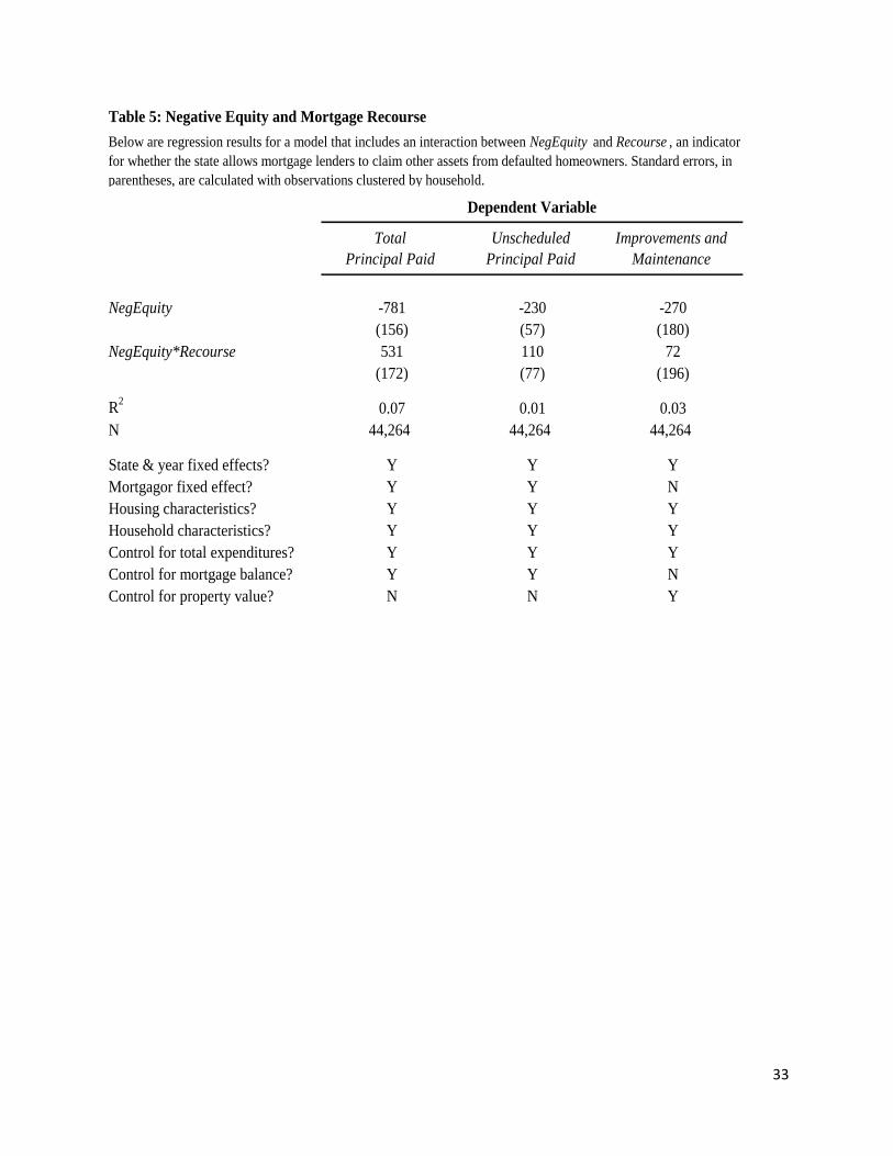
V.4 Foreclosure Laws, Lender Recourse and Negative Equity Effects

The analysis presented in Table 5 parses the main results, testing whether the spending

differences attributable to NegEquity vary with state foreclosure laws. The coefficient of interest

is the interaction term between NegEquity and Recourse, an indicator for whether the state

permits mortgage lenders to pursue borrowers’ other assets when the collateral value falls short

of the loan balance. Prediction 5 suggests that debt overhang matters less in recourse states and

that the interaction coefficient should be positive. The results offer weak confirmation that this is

21

the case for principal payments. The interaction coefficient is positive and significant at the 1%

level for total principal payments and positive but not quite significant (p-value 0.15) for

unscheduled payments. On the other hand, for improvements and maintenance the estimated

interaction coefficient is smaller and statistically insignificant.

V.5 Robustness

The analysis presented in Table 6 examines the robustness of the main findings. The first

two models use variations of the dependent variables: an indicator for any spending and log

spending. The second two models include additional control variables: MSA-year fixed effects

and a control for income. The results are broadly similar to the main findings, helping to address

any concerns about functional form assumptions, outliers in investment spending, left censoring

of the main dependent variables, and bias due to regional economic trends that affect negative

equity.

Looking at the extensive margin, negative equity homeowners are 1.1 percentage points

less likely to make any principal payment, 5 percentage points less likely to make principal

payments beyond the scheduled amount and 2.8 percentage points less likely to make

improvements. The latter two declines are substantial, with unscheduled principal payments

being 35 percent less likely and improvements being 10 percent less likely. The log-linear model

shows that among those making positive principal payments, negative equity homeowners pay

0.10 log points less, implying a roughly 10 percent decline as opposed to the 25 percent decline

in the main analysis. The log-linear results show an insignificant 12 percent decline in additional

principal payments, indicating that most of the decline in these payments occurs along the

22

extensive margin. For improvements, on the other hand, negative equity homeowners also reduce

spending on the intensive margin, with a 0.22 log point decline in spending.

The second set of models includes additional control variables. First, I confirm that

controlling for income does not change the main results. Second, I include MSA-year fixed

effects, a change that limits the sample to the 45% of observations for which I observe the

homeowner’s MSA (revealed for MSAs with population above 100,000). This model restricts the

identifying variation in negative equity by controlling for city-level trends, including trends in

housing markets. The negative equity coefficients are unchanged, which confirms that the main

results do not rely on a potentially flawed comparison across cities with very different real estate

markets.

V.6 Interpretation

In the extreme, debt overhang is unsurprising behavior. When a homeowner is days away

from default and certain of the outcome, it is not surprising that they do not invest in their home.

But the magnitude of the estimates in this analysis suggests that a much larger group of

homeowners is cutting back and doing so on a forward looking basis as they anticipate the

increased possibility, if not certainty, of default. Foreclosure starts peaked at a quarterly rate of

1.25% of loans, or 0.81% of homeowners after accounting for non-mortgagors. So, if each

homeowner going into foreclosure reduced to zero home improvement and maintenance

spending, average quarterly spending would fall by less than 1%, far below the 30% reduction

that I estimate.

23

VI. Conclusion

This paper extends our understanding of the financial decisions made by heavily indebted

homeowners, a topic of significance after the rapid rise in mortgage borrowing – a doubling

between 2000 and 2007 – and the substantial fall in U.S. home prices thereafter. For up to 15%

of homeowners, mortgage debts even exceed the value of their home. Finance theory predicts

that homeowners in these circumstances will underinvest, reducing both mortgage principal

payments and home improvement spending due to debt overhang.

Using detailed household-level data on housing expenditures, I test this hypothesis and

find that negative equity homeowners do indeed cut back on principal and improvements, by

roughly 30%. These differences do not reflect a general spending decline by negative equity

homeowners, nor are they limited to borrowing constrained households. Within the household,

the cutbacks are specific to durable investments in the physical structure, on which the mortgage

lender has a claim in foreclosure. Debt overhang best explains this set of facts.

The results suggest that national spending on home improvements, a sizeable component

of total housing investment, will be roughly 5% lower (15% of homeowners with negative equity

reducing spending by 30%) until the negative equity problem is resolved through price

appreciation, default or principal reduction. The estimates also imply that in a state like Nevada,

where the incidence of negative equity is 50%, home prices are likely to grow 5-10% slower

because of underinvestment.17

Finally, this analysis is helpful in assessing mortgage principal

reduction: provided that it restores positive equity, such a policy appears to improve

homeowners’ willingness to make mortgage payments and additional equity investments. An

17

Assumes 40-50% of price appreciation is driven by improvements. 50% negative equity*50% of

appreciation*30% reduction due to negative equity = 7.5% decline in growth rate.

24

interesting question for future empirical work is whether changes in mortgage debt overhang also

affect labor supply, as suggested by Mulligan(2008).

25

References

Bhutta, Neil, Jane Dokko, and Hui Shan. 2010. The Depth of Negative Equity and Mortgage

Default Decisions. Federal Reserve Board working paper, FEDS 2010-35.

Brady, Peter J., Glenn B. Canner, and Dean M. Maki. 2000. The Effects of Recent Mortgage

Refinancing. Federal Reserve Bulletin 86(7): 441-450.

Bucks, Brian K., Arthur B. Kennickell, Traci L. Mach and Kevin B. Moore. 2009. Changes in

U.S. Family Finances from 2004 to 2007: Evidence from the Survey of Consumer Finances.

Federal Reserve Bulletin 95(1): A1-A55.

Campbell, John Y., Stefano Giglio, and Parag Pathak. Forthcoming. Forced Sales and House

Prices. American Economic Review.

Chan, Sewin. 2001. Spatial Lock-in: Do Falling House Prices Constrain Residential Mobility?

Journal of Urban Economics 49(3): 567-586.

Davidoff, Thomas. 2006. Maintenance and the Home Equity of the Elderly. Working paper.

Deng, Yongheng, John M. Quigley, and Robert Van Order. 2000. Mortgage Terminations,

Heterogeneity and the Exercise of Mortgage Options. Econometrica 68(2): 275-308.

Deng, Yongheng, and Stuart A. Gabriel. 2006. Risk-Based Pricing and the Enhancement of

Mortgage Credit Availability among Underserved and Higher Credit-Risk Populations. Journal

of Money, Credit and Banking 38(6): 1431-1460.

26

Ferreira, Fernando, Joseph Gyourko, and Joseph Tracy. 2008. Housing Busts and Household

Mobility. Working paper.

Foote, Christopher L., Kristopher Gerardi, and Paul S. Willen. 2008. Negative equity and

foreclosure: Theory and evidence. Journal of Urban Economics 64(2): 234-245.

Ghent, Andra C., and Marianna Kudlyak. 2009. Recourse and Residential Mortgage Default:

Theory and Evidence from U.S. States. Federal Reserve Bank of Richmond Working Paper 09-

10.

Guiso, Luigi, Paola Sapienza, and Luigi Zingales. 2009. Moral and Social Constraints to

Strategic Default on Mortgages. Working Paper.

Gyourko, Joseph, and Joseph Tracy. 2006. Using Home Maintenance and Repairs to Smooth

Variable Earnings. The Review of Economics and Statistics 88(4): 736-747.

Haughwout, Andrew, Ebiere Okah, and Joseph Tracy. 2009. Second Chances: Subprime

Mortgage Modification and Re-Default. Federal Reserve Bank of New York Staff Report no.

417.

Hurst, Erik and, Frank Stafford. 2004. Home is Where the Equity is: Mortgage Refinancing and

Household Consumption. Journal of Money, Credit and Banking 36(6): 985-1014.

Keynes, John Maynard. 1920. The Economic Consequences of the Peace. New York: Harcourt,

Brace and Howe.

27

Krugman, Paul R. 1988. Financing vs. Forgiving a Debt Overhang. Journal of Development

Economics 29(3): 253-268.

Mendelsohn, Robert. 1977. Empirical Evidence on Home Improvements. Journal of Urban

Economics 4(): 459-468.

Mian, Atif and, Amir Sufi. Forthcoming. House Prices, Home Equity-Based Borrowing, and the

U.S. Household Leverage Crisis. American Economic Review.

Montgomery, Claire. 1992. Explaining Home Improvement in the Context of Household

Investment in Residential Housing. Journal of Urban Economics 32(1): 326-350.

Mulligan, Casey B. 2008. A Depressing Scenario: Mortgage Debt Becomes Unemployment

Insurance. NBER Working Paper 14514.

Myers, Stewart C. 1977. Determinants of Corporate Borrowing. Journal of Financial Economics

5(2): 147-175.

Olney, Martha L. 1999. Avoiding Default: The Role of Credit in the Consumption Collapse of

1930. Quarterly Journal of Economics 114(1): 319-335.

Pence, Karen M. 2006. Foreclosing on Opportunity: State Laws and Mortgage Credit. The

Review of Economics and Statistics 88(1): 177-182.

Sachs, Jeffrey D. 1990. A Strategy for Efficient Debt Reduction. Journal of Economic

Perspectives 4(1): 19-29.

28

Figure 1

Figure 2

akal

az

ca

co

ctde

fl

ga

hi

idil

in ksky

ma

md

mi

mnmo

ne

nhnj

nv

ny

oh

or

pasctn

tx

ut

va

wa wi

0.1

.2.3

.4.5

First A

me

rica

n N

ega

tive E

qu

ity (

%)

0 .05 .1 .15 .2CE Negative Equity (%)

pct_neg_equity_fa Fitted values

Note: Correlation of 0.7.

CE vs. First American

Proportion Negative Equity by State

0

200

400

600

800

Mean (

$)

0-0.250.25-0.5

0.5-0.750.75-1

1-1.251.25-1.5

1.5-1.751.75-2

Improvements and Maintenance

0

500

1,0

001,5

002,0

00

Mean (

$)

0-0.250.25-0.5

0.5-0.750.75-1

1-1.251.25-1.5

1.5-1.751.75-2

Principal Paid (Total)

050

100

150

200

250

Mean (

$)

0-0.250.25-0.5

0.5-0.750.75-1

1-1.251.25-1.5

1.5-1.751.75-2

Princpal Paid (Unscheduled)

Spending by Loan-to-value Category

29

Table 1: Summary Statistics, Stratified by Negative Equity

PANEL A: Housing Characteristics obs mean obs mean

Property value 53,555 296,629 2,116 216,800 *

Mortgagor (d) 53,555 0.65 2,116 0.99 *

Total mortgage 53,555 82,579 2,116 264,742 *

First mortgage 53,555 76,714 2,116 245,542 *

Home equity loan 53,555 1,786 2,116 8,717 *

Home equity LOC 53,555 4,079 2,116 10,484 *

Age of home 49,852 37.2 1,912 31.9 *

Years owned 52,270 14.4 2,074 6.1 *

Rooms 53,302 6.9 2,092 6.7 *

Bedrooms 53,311 3.2 2,095 3.3 *

Bathrooms 53,305 1.9 2,096 1.9

Central air (d) 53,491 0.69 2,109 0.74 *

Swimming pool (d) 53,491 0.11 2,109 0.11

Porch (d) 53,491 0.84 2,109 0.82 *

Off-street parking (d) 53,491 0.83 2,109 0.79 *

PANEL B: Household Characteristics

Income/Wealth

Annual income 51,758 72,154 2,039 71,235

Expenditures (qtr) 53,555 15,214 2,116 16,908 *

Liquid assets 28,126 37,094 1,031 9,637 *

Financial assets 26,411 120,700 997 39,789 *

Unsecured credit (2) 53,555 3,999 2,116 7,628 *

Unsecured credit (5) 20,224 8,505 898 13,000 *

Employment/Insurance

Weeks worked 53,551 38.2 2,116 45.8 *

Unempemployment ins. 51,375 98.4 2,018 79.5

Retired 53,555 0.24 2,116 0.07 *

Education

No high school degree 53,555 0.10 2,116 0.09

High school only 53,555 0.24 2,116 0.21 *

Some college 53,555 0.30 2,116 0.33 *

College degree 53,555 0.22 2,116 0.24

Graduate degree 53,555 0.15 2,116 0.13 *

Race/Ethnicity

White 53,555 0.80 2,116 0.68 *

Black 53,555 0.07 2,116 0.13 *

Hispanic 53,555 0.08 2,116 0.12 *

Asian 53,555 0.04 2,116 0.06 *

Other 53,555 0.01 2,116 0.02 *

Other

Age 53,555 53.3 2,116 43.6 *

Family size 53,555 2.7 2,116 3.2 *

NegEquity = 1NegEquity= 0 Diff. significant

at 5% level

30

Table 2: Negative Equity and Home Investments

Total

Principal Paid

Unscheduled

Principal Paid

Improvements &

Maintenance Improvements Maintenance

[1508] [219] [705] [614] [91]

NegEquity -367 -144 -215 -187 -27

(97) (54) (82) (81) (10)

Total expenditures 0.019 0.006 0.046 0.038 0.008

(0.003) (0.002) (0.006) (0.006) (0.001)

Property Value 0.001 0.001 0.00004

(0.0002) (0.0002) (0.00002)

Mortgage debt 0.003 0.0004

(0.0003) (0.0002)

R2

0.07 0.01 0.03 0.02 0.03

N 44,264 44,264 44,264 44,264 44,264

State & year fixed effects? Y Y Y Y Y

Mortgagor fixed effect? Y Y N N N

Housing characteristics? Y Y Y Y Y

Household characteristics? Y Y Y Y Y

Dependent Variable

[mean]

Below are OLS estimation results for regressions of principal payments, improvements and maintenance spending on an indicator for negative equity and

control variables. Standard errors, in parentheses, are calculated with observations clustered by household.

31

Table 3: Negative Equity Effects for Financially Unconstrained

Total

Principal Paid

Total

Principal Paid

Total

Principal Paid

Improvements &

Maintenance

Improvements &

Maintenance

Improvements &

Maintenance

[1684] [1857] [2136] [736] [966] [1134]

Sample: Unsec. Debt = 0 Income > 65K

Unsec. Debt = 0

& Income > 65K Unsec. Debt = 0 Income > 65K

Unsec. Debt = 0

& Income > 65K

NegEquity -489 -422 -745 -407 -194 -504

(197) (145) (306) (122) (135) (237)

Total expenditures 0.025 0.018 0.025 0.049 0.044 0.045

(0.006) (0.004) (0.008) (0.010) (0.008) (0.012)

Property Value 0.001 0.001 0.001

(0.0004) (0.0003) (0.0005)

Mortgage debt 0.004 0.003 0.003

(0.0006) (0.0004) (0.0007)

R2

0.10 0.06 0.08 0.03 0.03 0.03

N 19,041 24,177 9,190 19,041 24,177 9,190

State & year fixed effects? Y Y Y Y Y Y

Mortgagor fixed effect? Y Y Y N N N

Housing characteristics? Y Y Y Y Y Y

Household characteristics? Y Y Y Y Y Y

Dependent Variable

[mean]

This table presents regression coefficients estimated on subsets of the main sample, chosen to isolate households that are not financially constrained. Standard errors, in

parentheses, are calculated with observations clustered by household.

32

Table 4: Falsification, Negative Equity and Other Durables

Vehicles

Furniture and

Home Equipment

[981] [502]

NegEquity -55 -47

(56) (77)

Total expenditures 0.10 0.05

(0.01) (0.01)

Property Value -0.0001

(0.0001)

R2

0.16 0.12

N 48,366 44,264

State & year fixed effects? Y Y

Housing characteristics? N Y

Household characteristics? Y Y

Dependent Variable

[mean]

Below are estimation results from two falsification exercises, in which spending on vehicles and spending on other

property-related durables are regressed on the negative equity indicator and control variables. Standard errors, in

parentheses, are calculated with observations clustered by household.

33

Table 5: Negative Equity and Mortgage Recourse

Total

Principal Paid

Unscheduled

Principal Paid

Improvements and

Maintenance

NegEquity -781 -230 -270

(156) (57) (180)

NegEquity*Recourse 531 110 72

(172) (77) (196)

R2

0.07 0.01 0.03

N 44,264 44,264 44,264

State & year fixed effects? Y Y Y

Mortgagor fixed effect? Y Y N

Housing characteristics? Y Y Y

Household characteristics? Y Y Y

Control for total expenditures? Y Y Y

Control for mortgage balance? Y Y N

Control for property value? N N Y

Dependent Variable

Below are regression results for a model that includes an interaction between NegEquity and Recourse , an indicator

for whether the state allows mortgage lenders to claim other assets from defaulted homeowners. Standard errors, in

parentheses, are calculated with observations clustered by household.

34

Table 6: Robustness

Total

Principal Paid

Unscheduled

Principal Paid

Improvements &

Maintenance

Total

Principal Paid

Unscheduled

Principal Paid

Improvements &

Maintenance

[0.97] [0.14] [0.24] [6.70] [5.56] [6.48]

NegEquity -0.011 -0.050 -0.028 -0.10 -0.12 -0.22

(0.008) (0.010) (0.011) (0.03) (0.16) (0.09)

R2

0.86 0.07 0.03 0.26 0.12 0.10

N 44,264 44,264 44,264 29,164 4,357 10,514

Total

Principal Paid

Unscheduled

Principal Paid

Improvements &

Maintenance

Total

Principal Paid

Unscheduled

Principal Paid

Improvements &

Maintenance

[1509] [219] [705] [1712] [204] [818]

NegEquity -309 -127 -212 -440 -156 -303

(96) (53) (82) (159) (85) (106)

R2

0.08 0.01 0.03 0.09 0.01 0.04

N 44,264 44,264 44,264 19,404 19,404 19,404

State & year fixed effects? Y Y Y Y Y Y

Mortgagor fixed effect? Y Y N Y Y N

Housing characteristics? Y Y Y Y Y Y

Household characteristics? Y Y Y Y Y Y

Control for total expend.? Y Y Y Y Y Y

Control for mortgage bal.? Y Y N Y Y N

Control for property value? N N Y N N Y

Panel A shows regression results for variations on the dependent variables: linear probability models for any spending in columns 1 to 3 and a log-linear model in columns

4 to 6. Panel B shows results for a model that includes MSA-year fixed effects (columns 1 to 3) and a model that includes a control for income (column 4 to 6). Standard

errors in each model are shown in parentheses and are calculated with observations clustered by household.

--------------------With income control-------------------- ---------------With MSA-Year Fixed Effects---------------

Panel A

Panel B

----------------Indicator for any spending---------------- ----------------------------Logs----------------------------