1

Assigning real-time tasks on heterogeneous

multiprocessors with two unrelated types of processors

Gurulingesh Raravi · Björn Andersson · Konstantinos Bletsas

Abstract Consider the problem of partitioned scheduling of an implicit-deadline

sporadic task set on heterogeneous multiprocessors to meet all deadlines. Each pro-

cessor is either of type-1 or type-2. We present a new algorithm, FF-3C, for this

problem. FF-3C offers low time-complexity and provably good performance. Specif-

ically, FF-3C offers (i) a time-complexity of O(n · max(m, log n) + m · log m), where n is the number of tasks and m is the number of processors and (ii) the guarantee

that if a task set can be scheduled by an optimal partitioned-scheduling algorithm to

meet all deadlines then FF-3C meets all deadlines as well if given processors at most

1−α times as fast (referred to as speed competitive ratio) and tasks are scheduled using EDF; where α is a property of the task set. The parameter α is in the range

(0, 0.5] and for each task, it holds that its utilization is no greater than α or greater

than 1 − α on each processor type. Thus, the speed competitive ratio of FF-3C can never exceed 2.

We also present several extensions to FF-3C; these offer the same performance

guarantee and time-complexity but with improved average-case performance. Via

simulations, we compare the performance of our new algorithms and two state-of-

the-art algorithms (and variations of the latter). We evaluate algorithms based on

(i) running time and (ii) the necessary multiplication factor, i.e., the amount of extra

speed of processors that the algorithm needs, for a given task set, so as to succeed,

compared to an optimal task assignment algorithm. Overall, we observed that our new

algorithms perform significantly better than the state-of-the-art. We also observed that

our algorithms perform much better in practice, i.e., the necessary multiplication fac-

tor of the algorithms is much smaller than their speed competitive ratio. Finally, we

also present a clustered version of the new algorithm.

Keywords Bin packing · Heterogeneous multiprocessors · Real-time scheduling

1 Introduction

Designers have been achieving significant speedup of particular tasks by using spe-

cialized processing units (e.g., graphics processors for computer graphics or DSPs

for signal processing). The advent of heterogeneous multiprocessors on a single chip

facilitates this even more. Virtually all major manufacturers offer some kind of het-

erogeneous multiprocessor implemented on a single chip (AMD Inc 2011a; AMD

Inc 2011b; Freescale Semiconductor 2007; Gschwind et al. 2006; IBM Inc. 2005;

IEEE Spectrum 2011; Intel Corporation 2011; Maeda et al. 2005; NVIDIA 2011;

Texas Instruments 2011). Their use in embedded systems is non-trivial however be-

cause many embedded systems have real-time requirements, whose satisfaction at

run-time has to be proven/guaranteed a priori; this is a significant challenge for the

use of heterogeneous multicores. The way tasks are scheduled significantly influ-

ences whether their timing requirements are met. Unfortunately, for heterogeneous

multiprocessors, no comprehensive toolbox of real-time scheduling algorithms and

analysis techniques exists (unlike e.g., what exists for a uniprocessor).

An algorithm for deciding whether or not a task set can be scheduled on a

heterogeneous platform exists (Baruah 2004a) but it assumes that tasks can mi-

grate. This assumption, however, is often unrealistic in practice, since processors

with different functionalities typically have different instruction sets, register for-

mats, etc. Thus, the problem of assigning tasks to processors and then schedul-

ing them with a uniprocessor scheduling algorithm (i.e., without migration) is of

much greater practical significance. It requires solving two sub-problems: (i) assign-

ing tasks to processors and (ii) once tasks are assigned to processors, performing

uniprocessor scheduling on each processor. The latter problem is well-understood,

e.g., one may use an optimal scheduling algorithm1 such as EDF (Dertouzos 1974;

Liu and Layland 1973)—the difficult part is the task assignment.

Among known task assignment schemes for multiprocessors in general (i.e., not

necessarily heterogeneous), (i) bin-packing heuristics (e.g., first-fit), (ii) Integer Lin-

ear Programming (ILP) modeling, (iii) Linear Programming (LP) relaxation ap-

proaches for ILP and (iv) dynamic programming techniques perform provably well.

The task assignment problem on identical multiprocessors can be transformed into

a bin-packing problem. Bin-packing heuristics (Coffman et al. 1997) are popular for

1An optimal scheduling algorithm is one which always succeeds in finding a schedule in which all the

deadlines are met, if such a schedule exists.

task assignment but unfortunately, the proof techniques used on identical multipro-

cessors do not easily translate to heterogeneous multiprocessors. Traditionally, the

literature offered no bin-packing heuristic for assigning real-time tasks on heteroge-

neous multiprocessors. Instead, task assignment was modeled (Baruah 2004b, 2004c)

as Zero-One ILP. Such a formulation can be solved directly but has high computa-

tional complexity. In particular, the decision problem ILP is NP-complete and even

with knowledge of the structure of the constraints in the modeling of heterogeneous

multiprocessor scheduling, no polynomial-time algorithm is known (Garey and John-

son 1979, p. 245). Via relaxation of ILP formulation to LP and certain tricks (Potts

1985), polynomial time-complexity can be attained (Baruah 2004b, 2004c) (provided

that polynomial-time LP solver is used to solve the relaxed LP formulation). Neither

of the above two algorithms, however, attains low-degree (linear or quadratic) poly-

nomial time-complexity. It is a well-known fact that the problem under consideration

is equivalent to the problem of minimizing the makespan on unrelated machines.

For this problem, when the number of machines is fixed, a fully polynomial time

approximation scheme (FPTAS)2 was proposed in Horowitz and Sahni (1976). This

scheme required time O(nm(nm/E)m−1) and space O((nm/E)m−1) where m refers

to number of machines, n refers to number of jobs. Later, for the same problem (i.e.,

when the number of machines is fixed), a polynomial time approximation scheme

was proposed in Lenstra et al. (1990). However, the space requirement was signifi-

cantly improved compared to the algorithm proposed in Horowitz and Sahni (1976)

and was bounded by a polynomial which was a function of the input, m, and log(1/E).

The running time of the procedure was bounded by a function that is the product of

(n + 1)m/E where n is number of jobs. As we can see, neither of the above two algo- rithms achieves low-degree polynomial time- and space-complexity. Recently, Wiese

et al. (2012) proposed a PTAS for the problem of assigning tasks on a computing

platform comprising two or more types of processors. However, as any other PTAS,

this algorithm also has high degree polynomial time- and space-complexity.

In practice, many heterogeneous multiprocessors only use two types of processors.

For example, AMD (AMD Inc 2010), NVIDIA (IEEE Spectrum 2011), Intel (In-

tel Corporation 2011), FreeScale (Freescale Semiconductor 2007), TI (Texas Instru-

ments 2011) offer such chips. Traditionally, processors of the first type were meant

for general purpose computations and processors of the second type were meant for

special purpose computations (such as graphics or signal processing), hence task as-

signment was trivial. Today though, designers (Geer 2005) use processors of the sec-

ond kind for wide range of computations and this makes task assignment non-trivial.

Unfortunately, the literature did not provide any scheduling algorithm that took ad-

vantage of this special structure.

Therefore, in Andersson et al. (2010) (the conference version of this paper), we

considered the problem of non-migratively scheduling (also referred to as parti-

tioned scheduling) a set of independent implicit-deadline sporadic tasks, to meet

2A PTAS is an algorithm which produces a solution that is within a factor 1 + E of being optimal where E > 0 is a design parameter. The run time of a PTAS is polynomial in the input size (e.g., number of jobs)

and may be exponential in 1/E. A FPTAS is a PTAS with a running time that is polynomial both in input

size and 1/E.

all deadlines, on a heterogeneous multiprocessor where each processor is either of

type-1 or type-2 (with each task having different execution time on each proces-

sor type). We presented a new algorithm, FF-3C, for this problem—this algorithm

uses a bin-packing heuristic for assigning tasks. FF-3C offered low time-complexity

and provably good performance. Specifically, FF-3C offered (i) a time-complexity of

O(n · max(m, log n) + m · log m), where n denotes number of tasks and m denotes number of processors and (ii) the guarantee that if a task set can be scheduled by

an optimal task assignment algorithm to meet deadlines then FF-3C meets deadlines

as well if the given processors are twice as fast (referred to as the speed competitive

ratio) and tasks are scheduled using preemptive EDF scheduling algorithm. We also

presented several extensions to FF-3C; these offered the same time-complexity and

performance guarantee but in addition, they offered improved average-case perfor-

mance. Via experiments with randomly generated task sets, we compared the perfor-

mance of our algorithms and two established state-of-the-art algorithms (and varia-

tions of the latter) (Baruah 2004b, 2004c). We evaluated algorithms based on (i) av-

erage running time and (ii) the necessary multiplication factor, i.e., the amount of

extra speed of processors the algorithm needs, for a task set, in order to succeed as

compared to an optimal task assignment algorithm. Overall our new algorithms com-

pared favorably to the state-of-the-art.3 In particular, in our experimental evaluations,

one of our new algorithms, FF-4C-COMB, ran 12000 to 160000 times faster and

had significantly smaller necessary multiplication factor than state-of-the-art (Baruah

2004b, 2004c).

It is known in bin-packing that packing small items (i.e., tasks with small uti-

lizations) allows better performance bounds. Our conference paper, however, did

not exploit this. Hence, this article extends our conference paper (Andersson et al.

2010) by incorporating this idea among other things. The additional contributions

in this paper can be summarized as follows: (i) we improve the analysis of FF-3C

by incorporating the task parameters into analysis. Consider a task set in which, for

each task, it holds that its utilization is no greater than α or greater than 1-α on a

processor of type-1 and its utilization is no greater than α or greater than 1-α on

a processor of type-2. For such task sets, we show that FF-3C succeeds in meeting

all deadlines if it is possible to meet all deadlines by an optimal task assignment on

a computer platform where each processor has the speed 1-α of the corresponding

processor that FF-3C uses; (ii) we also prove the performance guarantee as a func-

tion of α for the algorithms with improved average-case performance (i.e., FF-4C,

FF-4C-NTC and FF-4C-COMB); (iii) we perform additional experiments to show

the performance of our algorithms with this new analysis. We have also (re-)run the

experiments that were carried out in Andersson et al. (2010) for evaluating the per-

formance of our algorithms with state-of-the-art (Baruah 2004b, 2004c) and (iv) we

also present a version of the new algorithm targeted for two-type platform where pro-

cessors are organized into clusters and task migration is allowed between processors

of the same cluster.

3For a given problem instance, the necessary multiplication factor of an algorithm is upper bounded by

its speed competitive ratio. If an algorithm has low necessary multiplication factor (compared to its speed

competitive ratio) for the vast majority of task sets then it indicates that the algorithm performs well.

i

i

i ∈ [ ] i

In the remainder of this paper, Sect. 2 offers necessary preliminaries. Section 3

presents some previously known and some new results that we use in Sect. 4, where

we formulate the new algorithm namely, FF-3C, and prove its performance. Sec-

tion 5 considers time-complexity. Section 6 describes the enhancements to FF-3C to

obtain better average-case performance and proves their performance. Section 7 of-

fers experimental evaluation; Sect. 8 presents a clustered version of FF-3C and finally

Sect. 9 concludes.

2 Preliminaries

In a computer platform with two unrelated types of processors, let P 1 be the set of

type-1 processors and P 2 be the set of type-2 processors. The workload consists of τ ,

a set of implicit-deadline sporadic tasks (i.e., for each task, its deadline is equal to its

minimum inter-arrival time) each of which releases a (potentially infinite) sequence

of jobs.

A task is assigned to a processor and all jobs released by this task must execute there. The utilization of task τi depends on the type of processor to which it is as-

signed. The utilization of task τi is u1 if τi is assigned to a type-1 processor. Anal-

ogously, the utilization of task τi is u2 if τi is assigned to a type-2 processor. Note that we allow u1 =∞ (resp., u2 = ∞) if task τi cannot be assigned at all to a type-1

i i

(resp., type-2) processor.

We assume that tasks are assigned unique identifiers. This allows two tasks with the same parameters to be in a set. For example, with u1 = 0.2, u2 = 0.4 and

i i u1 2

j = 0.2, uj = 0.4, we can form the set {τi, τj }. We also assume that processors

are assigned unique identifiers. This assumption is instrumental because if we sort

processors in ascending order of their identifiers then we can be sure that, when ap-

plying normal bin-packing schemes (e.g., first-fit) repeatedly on the same task set,

with tasks ordered in the same way, the bin-packing scheme outputs the same task

assignment for each run.

Let τ [p] denote the set of tasks assigned to a processor p. Earliest-Deadline- First (EDF) is a very popular algorithm in uniprocessor scheduling (Liu and Layland

1973). A slight adaptation of a previously known result (Liu and Layland 1973) gives

us:

Lemma 1 If all tasks in τ [p] are scheduled under EDF on a processor p (which is

of type-z, where z ∈ {1, 2}) and J,

τ τ p uz ≤ 1, then all deadlines are met.

Then the necessary and sufficient set of conditions for schedulability on a parti-

tioned heterogeneous multiprocessor with two types of processor is the following:

Thus our problem of scheduling tasks on a heterogeneous multiprocessor with two

types of processors is reduced to assigning tasks to processors such that the above

constraints are satisfied. Yet, even in the special case of identical multiprocessors,

this problem is intractable (Baruah 2004b). We therefore aim for a non-optimal algo-

rithm of low-degree polynomial time-complexity which would still offer good per-

formance.

Commonly, the performance of an algorithm is characterized using the notion of

the utilization bound (Liu and Layland 1973): an algorithm with a utilization bound

of UB is always capable of scheduling any task set with a utilization up to UB so

as to meet all deadlines. This definition has been used in uniprocessor scheduling

(Liu and Layland 1973) and multiprocessors with identical processors (Andersson et

al. 2001). However, it does not translate to heterogeneous multiprocessors, hence we

rely on the resource augmentation framework to characterize the performance of the

algorithm under design.

The speed competitive ratio CPTA of a non-migrative algorithm A is defined as

the lowest number such that for every task set τ and computing platform Π , it holds

that if it is possible for a non-migrative algorithm to meet all deadlines of τ on Π ,

then algorithm A meets all deadlines of τ on a platform Π whose every processor is

CPTA times faster than the corresponding processor in Π ,.4

A low speed competitive ratio indicates high performance; the best achievable is 1.

If a scheduling algorithm has an infinite speed competitive ratio then a task set exists

which could be scheduled (by another algorithm) to meet deadlines but would miss

deadlines with the actually used algorithm even if processor speeds were multiplied

by an “infinite” factor. Therefore, we aim for an algorithm with finite (ideally small)

speed competitive ratio.

We now introduce few notations that will be used later (from Sect. 4.3 onwards)

while proving the speed competitive ratio of our algorithms.

Let Π (|P 1|, |P 2|) denote a two-type heterogeneous platform comprising |P 1|

processors of type-1 and |P 2| processors of type-2. Let Π (|P 1|, |P 2|) × (s1, s2) de- note a two-type heterogeneous platform in which the speed of every processor of

type-1 is s1 times the speed of a type-1 processor in Π (|P 1|, |P 2|) and the speed of

every processor of type-2 is s2 times the speed of a type-2 processor in Π (|P 1|, |P 2|) where s1 and s2 are positive real-numbers (i.e., s1 > 0 and s2 > 0).

Let sched(A,τ,Π(|P 1|, |P 2|) × (s1, s2)) denote a predicate to signify that a task set τ meets all its deadlines when scheduled by an algorithm A on a two-type het-

erogeneous multiprocessor platform—Π (|P 1|, |P 2|) × (s1, s2). The term meets all its deadlines in this and other predicates means ‘meets deadlines for every possible

arrival of tasks that is valid as per the given parameters of τ ’.

We use sched(nmo-feasible,τ,Π(|P 1|, |P 2|) × (s1, s2)) to signify that there exists a non-migrative-offline-feasible preemptive schedule which meets all deadlines for

the specified system. Here, non-migrative schedule refers to a schedule in which all

the jobs of a task execute on the same processor on which the task has been assigned

4Our notion of speed competitive ratio in this paper is equivalent to that in previous work (Baruah 2004a).

It differs from that used in Andersson and Tovar (2007b). Other authors refer to speed competitive ratio as

resource augmentation bound.

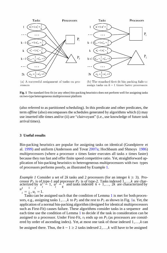
Fig. 1 The standard first-fit (or any other) bin-packing heuristics does not perform well for assigning tasks

on two-type heterogeneous multiprocessor platform

(also referred to as partitioned scheduling). In this predicate and other predicates, the

term offline (also) encompasses the schedules generated by algorithms which (i) may

use inserted idle times and/or (ii) are “clairvoyant” (i.e., use knowledge of future task

arrival times).

3 Useful results

Bin-packing heuristics are popular for assigning tasks on identical (Grandpierre et

al. 1999) and uniform (Andersson and Tovar 2007a; Hochbaum and Shmoys 1986)

multiprocessors (where a processor x times faster executes all tasks x times faster)

because they run fast and offer finite speed competitive ratio. Yet, straightforward ap-

plication of bin-packing heuristics to heterogeneous multiprocessors with two types

of processors performs poorly, as illustrated by Example 1.

Example 1 Consider a set of 2k tasks and 2 processors (for an integer k ≥ 3). Pro- cessor P1 is of type-1 and processor P2 is of type-2. Tasks indexed 1 , .. .,k are char- acterized by u1 = 1, u2 = 1 and tasks indexed k + 1 ,..., 2k are characterized by

i i k u1 1 2

i = k , ui = 1. Tasks can be assigned such that the condition of Lemma 1 is met for both proces-

sors, e.g., assigning tasks 1 , .. .,k to P2 and the rest to P1 as shown in Fig. 1a. Yet, the

application of a normal bin-packing algorithm (designed for identical multiprocessors

such as First-Fit) causes failure. These algorithms consider tasks in a sequence and each time use the condition of Lemma 1 to decide if the task in consideration can be

assigned to a processor. Under First-Fit, τ1 ends up on P1 (as processors are consid-

ered by order of ascending index). Yet, at most one task of those indexed 1 ,. .. ,k can

be assigned there. Thus, the k − 1 ≥ 2 tasks indexed 2 , .. .,k will have to be assigned

i

i

to P2. Next, the bin-packing scheme tries to assign tasks k + 1 ,..., 2k to P2; none fits and the algorithm fails.

Let us now provide the bin-packing algorithm with processors k − 1 times faster.

Then, tasks indexed 1 , . . .,k − 1 will be assigned to P1 and the kth task to P2 before

considering tasks indexed k + 1 ,..., 2k. Of the latter, many can be assigned to P 2

but not all and, since none can be assigned to P 1, the bin-packing algorithm would again fail as shown in Fig. 1b.

This holds for any k ≥ 3. For k → ∞, we see that the speed competitive ratio of such bin-packing schemes is infinite.

It can be seen that the cause of low performance of such a bin-packing scheme is

that, by considering tasks one by one, it lacks a “global view” of the problem, hence

may assign a task to a processor where it executes slowly. It seems a good idea to try

to assign each task to the processor where it executes faster. We will use this idea; let

us thus introduce the following definitions:

P 1 is the set of type-1 processors and P 2 is the set of type-2 processors. The task

set τ is viewed as two disjoint subsets, τ 1 and τ 2. The set τ 1 consists of those tasks

which run at least as fast on a type-1 processor as on a type-2 processor; τ 2 consists

of all other tasks. In notation:

We now list two useful observations along with their proofs.

Lemma 2 If there is a task τi in τ 1 such that 1 < u1, it is then impossible to meet all

deadlines with partitioning. Likewise for a task τi in τ 2 with 1 < u2.

Proof Intuitively, if the execution time of τi exceeds its deadline on processor type

where it runs fastest, it cannot be assigned anywhere to meet deadlines. D

Lemma 3 It is impossible to meet all deadlines if

Proof

The proof is by contradiction. Let τ be a task set for which Inequality (6) holds

and for which a feasible partitioning exists. Given that τ is feasible, the set of

constraints expressed by Inequalities (1) and (2) must hold. Then, respectively from

those inequalities, we have:

w ≥ wi 1 ∀i ∈

i 1 i=1

However, from Inequalities (5) and (4) respectively:

Then, respectively:

We can combine Inequalities (11) and (12) into:

Via summation of Inequality (13) over all p we obtain

1

This contradicts Inequality

(6). D

We next highlight how the problem in consideration is related to fractional knap-

sack problem, to help with proofs later. If you read this paper for the first time, you

may want to skip this section now and revisit it later.

Fractional Knapsack Problem: A vector x has n elements. The problem instance is represented by vectors v and w of real numbers, arranged such that

vi i

vi+1

+

{1, 2,...,n−1}. (Intuitively, vi and wi may be thought of as, respectively, the “value” and “weight” of an element.) Consider the problem of assigning values to the ele- ments in vector x so as to maximize

J,n = xi · vi subject to

J,n xi · wi ≤ CAP

where xi is a real number such that 0 ≤ xi ≤ 1 and CAP is a given upper bound. (Intuitively, determine how much of each item to use such that cumulative value

is maximized, subject to cumulative weight not exceeding some bound.)

Lemma 4 An optimal solution to the Fractional Knapsack Problem is obtained by

Algorithm 1.

Proof This is found in textbooks (Chap. 16.2 (Cormen et al. 2001)). D

2

u1 u1

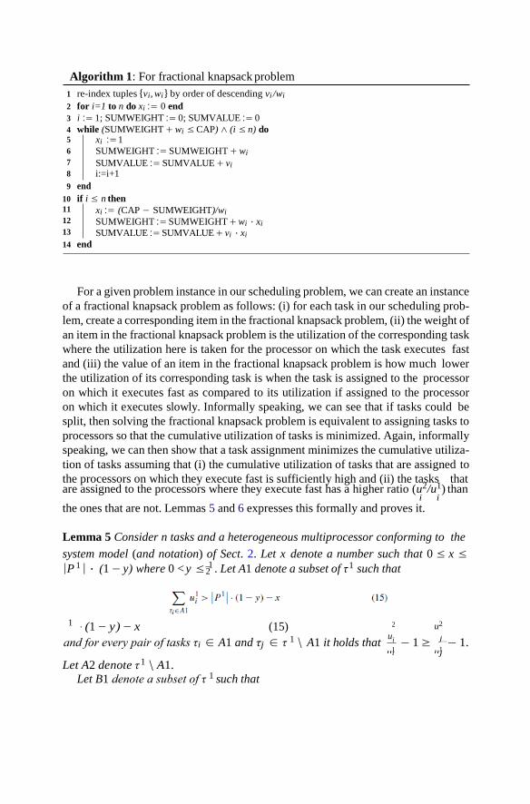
Algorithm 1: For fractional knapsack problem

1 re-index tuples {vi, wi } by order of descending vi /wi

2 for i=1 to n do xi := 0 end

3 i := 1; SUMWEIGHT := 0; SUMVALUE := 0

4 while (SUMWEIGHT + wi ≤ CAP) ∧ (i ≤ n) do 5

6

7

8

9 end

xi := 1

SUMWEIGHT := SUMWEIGHT + wi

SUMVALUE := SUMVALUE + vi

i:=i+1

10 if i ≤ n then 11

12

13

14 end

xi := (CAP − SUMWEIGHT)/wi

SUMWEIGHT := SUMWEIGHT + wi · xi

SUMVALUE := SUMVALUE + vi · xi

For a given problem instance in our scheduling problem, we can create an instance

of a fractional knapsack problem as follows: (i) for each task in our scheduling prob-

lem, create a corresponding item in the fractional knapsack problem, (ii) the weight of

an item in the fractional knapsack problem is the utilization of the corresponding task

where the utilization here is taken for the processor on which the task executes fast

and (iii) the value of an item in the fractional knapsack problem is how much lower

the utilization of its corresponding task is when the task is assigned to the processor

on which it executes fast as compared to its utilization if assigned to the processor

on which it executes slowly. Informally speaking, we can see that if tasks could be

split, then solving the fractional knapsack problem is equivalent to assigning tasks to

processors so that the cumulative utilization of tasks is minimized. Again, informally

speaking, we can then show that a task assignment minimizes the cumulative utiliza-

tion of tasks assuming that (i) the cumulative utilization of tasks that are assigned to

the processors on which they execute fast is sufficiently high and (ii) the tasks that are assigned to the processors where they execute fast has a higher ratio (u2/u1) than

i i

the ones that are not. Lemmas 5 and 6 expresses this formally and proves it.

Lemma 5 Consider n tasks and a heterogeneous multiprocessor conforming to the

system model (and notation) of Sect. 2. Let x denote a number such that 0 ≤ x ≤ |P 1 |· (1 − y) where 0 <y ≤ 1 . Let A1 denote a subset of τ 1 such that

1 · (1 − y) − x (15)

2 u2

and for every pair of tasks τi ∈ A1 and τj ∈ τ 1 \ A1 it holds that ui

i

− 1 ≥ j − 1. j

Let A2 denote τ 1 \ A1.

Let B1 denote a subset of τ 1 such that

τi ∈B1

u1 1

P (1 − y) − x (16) ≤ · i

i

u

Let B2 denote τ \ B1. It then holds that:

1

Proof Let us arbitrarily choose A1, B1 as defined. We will prove that this implies

Inequality (17). Using Inequalities (15) and (16) we clearly get:

With this choice of A1 and B1, let us consider different instances of the fractional

knapsack problem:

Instance1: CAP = left-hand side of Inequality (18). For each τi ∈ τ , create an item i with vi = u2 − u1 and wi = u1

i i i

SUMVALUE1 = value of variable SUMVALUE when Algorithm 1 terminates with Instance1 as input.

Instance2: CAP = left-hand side of Inequality (18). For each τi ∈ A1, create an item i with vi = u2 − u1 and wi = u1

i i i

SUMVALUE2 = value of variable SUMVALUE when Algorithm 1 terminates with Instance2 as input.

Instance3: CAP = right-hand side of Inequality (18). For each τi ∈ B1, create an item i with vi = u2 − u1 and wi = u1

i i i

SUMVALUE3 = value of variable SUMVALUE when Algorithm 1 terminates with Instance3 as input.

Instance4: CAP = right-hand side of Inequality (18). For each τi ∈ τ , create an item i with vi = u2 − u1 and wi = u1

i i i

SUMVALUE4 = value of variable SUMVALUE when Algorithm 1 terminates with Instance4 as input.

Observe that:

O1: In all four instances, it holds for each element that vi

wi

O2: Instance1 and Instance2 have the same capacity.

u2

= 1 − 1. i

O3: Although Instance2 has a subset of the elements of Instance1, this subset is the

subset of those elements with the largest vi /wi —follows from definition of A1.

O4: CAP in Instance2 is exactly the sum of the weights of the elements in A1.

O5: From O1,O2,O3 and O4: SUMVALUE2 = SUMVALUE1. O6: Instance3 and Instance4 have the same capacity.

O7: Instance3 has a subset of the elements of Instance4.

O8: From O6 and O7: SUMVALUE3 ≤ SUMVALUE4.

O9: Instance4 has smaller capacity than Instance1. O10: Instance4 has the same elements as Instance1.

τi ∈B1

u1 1

P (1 − y) − x (16) ≤ · i

O11: From O9 and O10: SUMVALUE4 ≤ SUMVALUE1.

O12: From O8 and O11: SUMVALUE3 ≤ SUMVALUE1.

13: From O12 and O5: SUMVALUE3 ≤ SUMVALUE2.

2

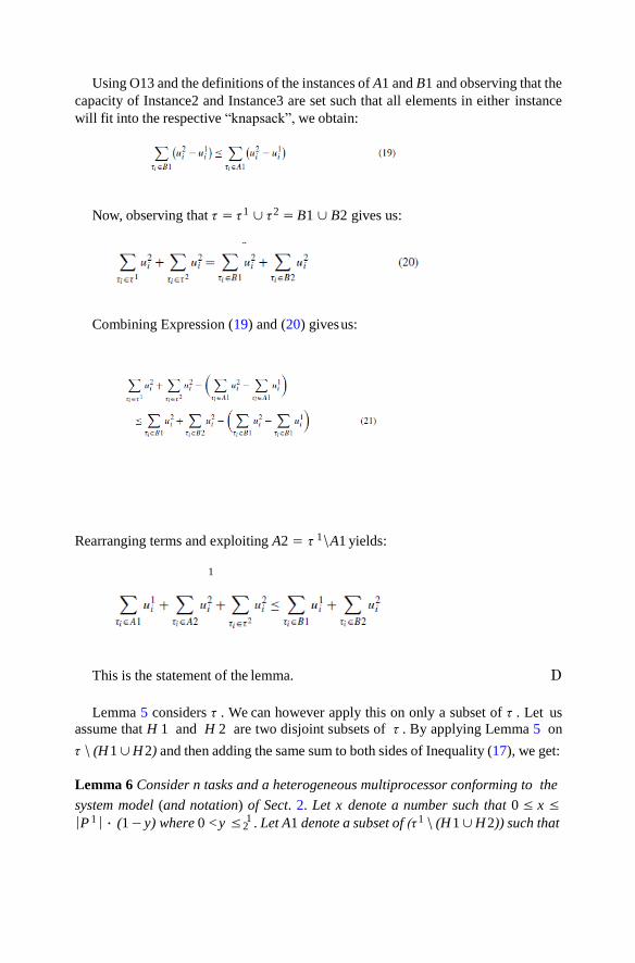
Using O13 and the definitions of the instances of A1 and B1 and observing that the

capacity of Instance2 and Instance3 are set such that all elements in either instance

will fit into the respective “knapsack”, we obtain:

Now, observing that τ = τ 1 ∪ τ 2 = B1 ∪ B2 gives us:

2

Combining Expression (19) and (20) gives us:

Rearranging terms and exploiting A2 = τ 1\A1 yields:

1

This is the statement of the lemma. D

Lemma 5 considers τ . We can however apply this on only a subset of τ . Let us

assume that H 1 and H 2 are two disjoint subsets of τ . By applying Lemma 5 on

τ \ (H 1 ∪ H 2) and then adding the same sum to both sides of Inequality (17), we get:

Lemma 6 Consider n tasks and a heterogeneous multiprocessor conforming to the

system model (and notation) of Sect. 2. Let x denote a number such that 0 ≤ x ≤

|P 1|· (1 − y) where 0 <y ≤ 1 . Let A1 denote a subset of (τ 1 \ (H 1 ∪ H 2)) such that

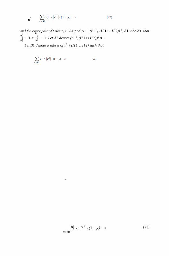
τi ∈B1

u1 1

P (1 − y) − x (23) ≤ · i

i j

u1

and for every pair of tasks τi ∈ A1 and τj ∈ (τ 1 \ (H 1 ∪ H 2)) \ A1 it holds that

u2

u2 1

u1 − 1 ≥ u1 − 1. Let A2 denote (τ \ (H 1 ∪ H 2))\A1.

i j

Let B1 denote a subset of τ 1 \ (H 1 ∪ H 2) such that

2

2

2

2

Let B2 denote (τ \ (H 1 ∪ H 2))\B1. It then holds that:

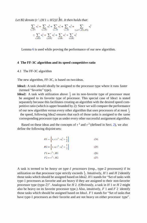
Lemma 6 is used while proving the performance of our new algorithm.

4 The FF-3C algorithm and its speed competitive ratio

4.1 The FF-3C algorithm

The new algorithm, FF-3C, is based on two ideas.

Idea1: A task should ideally be assigned to the processor type where it runs faster

(termed “favorite” type).

Idea2: A task with utilization above 1 on its non-favorite type of processor must

be assigned to its favorite type of processor. This special case of Idea1 is stated

separately because this facilitates creating an algorithm with the desired speed com-

petitive ratio (which is upper bounded by 2): Since we will compare the performance

of our new algorithm versus every other algorithm that uses processors of at most 1

the speed, following Idea2 ensures that each of those tasks is assigned to the same

corresponding processor type as under every other successful assignment algorithm.

Based on these ideas and the concepts of τ 1 and τ 2 (defined in Sect. 2), we also

define the following disjoint sets:

A task is termed to be heavy on type-1 processors (resp., type-2 processors) if its

utilization on that processor type strictly exceeds 1 . Intuitively, H 1 and H 2 identify

those tasks which should be assigned based on Idea2. H 1 stands for “Set of tasks with

type-1 processors as favorite and are heavy if they are assigned to their non-favorite

processor type (type-2)”. Analogous for H 2. (Obviously, a task in H 1 or H 2 might

also be heavy on its favorite processor type.) Also, intuitively, F 1 and F 2 identify

those tasks which should be assigned based on Idea1. F 1 stands for “Set of tasks that

have type-1 processors as their favorite and are not heavy on either processor type”.

Analogous for F 2. From the definitions of H 1, H 2, F 1, F 2 (and Inequalities (4)

and (5)), we have:

Algorithm 2 shows the pseudo-code of the new algorithm FF-3C. The intuition be-

hind the design of FF-3C is that first we assign tasks to their favorite processors which

would be heavy on other processor type (Lines 4–5). Then we assign the non-heavy

tasks to their favorite processors (Lines 6–7). Then, if there are remaining non-heavy

tasks, these have to be assigned to processors that are not their favorite (Lines 12

and 20).

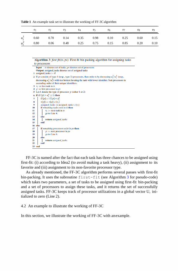
Table 1 An example task set to illustrate the working of FF-3C algorithm

1 i 2 i

FF-3C is named after the fact that each task has three chances to be assigned using

first-fit: (i) according to Idea2 (to avoid making a task heavy), (ii) assignment to its

favorite and (iii) assignment to its non-favorite processor type.

As already mentioned, the FF-3C algorithm performs several passes with first-fit

bin-packing. It uses the subroutine first-fit (see Algorithm 3 for pseudo-code)

which takes two parameters, a set of tasks to be assigned using first-fit bin-packing

and a set of processors to assign these tasks, and it returns the set of successfully

assigned tasks. FF-3C keeps track of processor utilizations in a global vector U, ini-

tialized to zero (Line 2).

4.2 An example to illustrate the working of FF-3C

In this section, we illustrate the working of FF-3C with an example.

u

u

τ1 τ2 τ3 τ4 τ5 τ6 τ7 τ8 τ9

0.60 0.70 0.14 0.35 0.98 0.10 0.25 0.60 0.15

0.80 0.06 0.48 0.25 0.75 0.15 0.85 0.20 0.10

Example 2 Consider a two-type heterogeneous multiprocessor platform with one

processor of type-1 (namely, P1) and two processors of type-2 (namely, P2 and P3)

and a task set as shown in Table 1. Let us see how FF-3C assigns the task set

to processors. The task set τ is partitioned as follows: τ 1 = {τ1, τ3, τ6, τ7} and

τ 2 = {τ2, τ4, τ5, τ8, τ9}—see Inequalities (4). On Line 1, FF-3C (pseudo-code shown in Algorithm 2) forms sets H 1, H 2, F 1 and F 2 (as defined by Inequalities (24)–(27))

as follows: H 1 = {τ1, τ7}, H 2 = {τ2, τ5, τ8}, F 1 = {τ3, τ6} and F 2 = {τ4, τ9}. On Line 4, FF-3C calls first-fit sub-routine (shown in Algorithm 3) to assign tasks

in H 1 = {τ1, τ7} on processor P1 (of type-1). The first-fit sub-routine (on Line 2 in Algorithm 3) sorts the tasks in H 1 in descending order of u2/u1, i.e., (τ7, τ1). The

i i

sub-routine successfully assigns both the tasks in H 1 to processor P1. After assigning H 1 tasks, the remaining utilization of processor P1 is 0.15.

On Line 5, FF-3C calls first-fit sub-routine to assign tasks in H 2 = {τ2, τ5, τ8} on processor P2 and P3 (of type-2). The first-fit sub-routine sorts the tasks in H 2 in ascending order of u2/u1, i.e., (τ2, τ8, τ5). The sub-routine successfully assigns τ2

i i

and τ8 to processor P2 (but fails to assign τ5 to P2) and τ5 to processor P3. After as- signing H 2 tasks, the remaining utilization of processor P2 is 0.74 and the remaining

utilization of processor P3 is 0.25.

On Line 6, FF-3C calls first-fit sub-routine to assign tasks in F 1 = {τ3, τ6} on processor P1 (of type-1). The first-fit sub-routine sorts the tasks in F 1 in descending order of u2/u1, i.e., (τ3, τ6). The sub-routine successfully assigns the task τ3 to P1 but

i i

fails to assign τ6 to P1 as there is not enough capacity left in P1. After assigning τ3, the remaining utilization of processor P1 is 0.01. Hence, when first-fit returns on

Line 6, we have: F 11 = {τ3}. On Line 7, FF-3C calls first-fit sub-routine to assign tasks in F 2 = {τ4, τ9} on pro-

cessors P2 and P3 (of type-2). The first-fit sub-routine (on Line 2 in Algorithm 3) sorts the tasks in F 2 in ascending order of u2/u1, i.e., (τ9, τ4). The sub-routine suc-

i i

cessfully assigns both the tasks in F 2 to processor P2. After assigning τ9 and τ4, the remaining utilization of processor P2 is 0.39. Hence, when first-fit returns on Line 7,

we have: F 22 = {τ4, τ9}.

The condition on Line 10, i.e., (F 11 /= F 1) ∧ (F 22 = F 2) is TRUE and hence,

new task set F 12 is formed on Line 11, i.e., F 12 = {τ6}. FF-3C on Line 12 calls first-fit sub-routine to assign tasks in F 12 to processors P2 and P3 (of type-2). The

first-fit sub-routine successfully assigns the single task τ6 of F 12 to processors P2.

The remaining utilization of processor P2 is 0.24. Since the sub-routine managed to

assign all tasks in F 12 to type-2 processors, FF-3C declares SUCCESS on Line 13.

So, the final assignment of tasks to processors looks as follows: τ1, τ3 and τ7 are

assigned to processor P1 (of type-1), τ2, τ4, τ6, τ8 and τ9 are assigned to processor

P2 (of type-2) and τ5 is assigned to processor P3 (of type-2).

4.3 The speed competitive ratio of FF-3C

In this section, we will prove the speed competitive ratio of FF-3C. We will derive its

speed competitive ratio in terms of a task set parameter, namely α. The parameter α

is a property of the task set on which FF-3C is applied and it reflects the values that

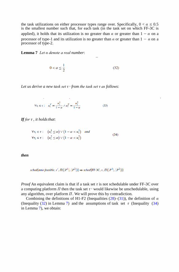
the task utilizations on either processor types range over. Specifically, 0 < α ≤ 0.5 is the smallest number such that, for each task (in the task set on which FF-3C is

applied), it holds that its utilization is no greater than α or greater than 1 − α on a

processor of type-1 and its utilization is no greater than α or greater than 1 − α on a processor of type-2.

Lemma 7 Let α denote a real number:

Let us derive a new task set τ , from the task set τ as follows:

,

If for τ , it holds that:

then

Proof An equivalent claim is that if a task set τ is not schedulable under FF-3C over

a computing platform Π then the task set τ , would likewise be unschedulable, using

any algorithm, over platform Π . We will prove this by contradiction.

Combining the definitions of H1-F2 (Inequalities (28)–(31)), the definition of α

(Inequality (32) in Lemma 7) and the assumptions of task set τ (Inequality (34)

in Lemma 7), we obtain:

Assume that FF-3C failed to assign τ on Π but it is possible (using an algorithm

OPT) to assign τ , on Π . Since FF-3C failed to assign τ on Π , it must have declared

FAILURE. We explore all possibilities for the failure of FF-3C to occur:

i

i

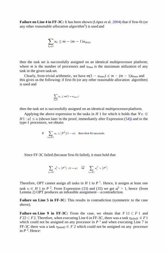
Failure on Line 4 in FF-3C: It has been shown (López et al. 2004) that if first-fit (or

any other reasonable allocation algorithm5) is used and

then the task set is successfully assigned on an identical multiprocessor platform;

where m is the number of processors and umax is the maximum utilization of any

task in the given task set.

Clearly, from trivial arithmetic, we have m(1 − umax) ≤ m − (m − 1)umax and this gives us the following: if first-fit (or any other reasonable allocation algorithm)

is used and

then the task set is successfully assigned on an identical multiprocessor platform.

Applying the above expression to the tasks in H 1 for which it holds that ∀τi ∈

H 1 : u1 ≤ α (shown later in the proof, immediately after Expression (54)) and to the type-1 processors, we obtain:

Since FF-3C failed (because first-fit failed), it must hold that

Therefore, OPT cannot assign all tasks in H 1 to P 1. Hence, it assigns at least one

task τi ∈ H 1 to P 2. From Expression (33) and (35) we get u2, > 1, hence (from

Lemma 2) OPT produces an infeasible assignment—a contradiction.

Failure on Line 5 in FF-3C: This results in contradiction (symmetric to the case

above).

Failure on Line 9 in FF-3C: From the case, we obtain that F 11 ⊂ F 1 and

F 22 ⊂ F 2. Therefore, when executing Line 6 in FF-3C, there was a task τfailed1 ∈ F 1 which could not be assigned on any processor in P 1 and when executing Line 7 in

FF-3C there was a task τfailed2 ∈ F 2 which could not be assigned on any processor in P 2. Hence:

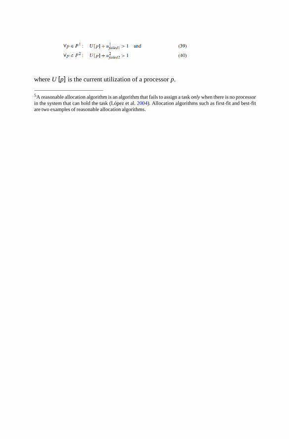
where U [p] is the current utilization of a processor p.

5A reasonable allocation algorithm is an algorithm that fails to assign a task only when there is no processor

in the system that can hold the task (López et al. 2004). Allocation algorithms such as first-fit and best-fit

are two examples of reasonable allocation algorithms.

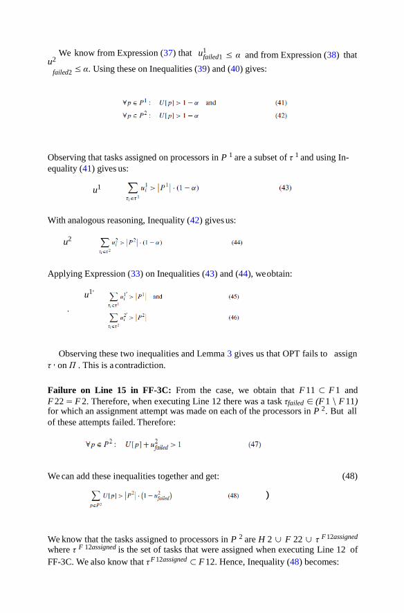
failed1 We know from Expression (37) that u1

u2 ≤ α and from Expression (38) that

failed2 ≤ α. Using these on Inequalities (39) and (40) gives:

Observing that tasks assigned on processors in P 1 are a subset of τ 1 and using In-

equality (41) gives us:

u1

With analogous reasoning, Inequality (42) gives us:

u2

Applying Expression (33) on Inequalities (43) and (44), we obtain:

u1,

,

Observing these two inequalities and Lemma 3 gives us that OPT fails to assign

τ , on Π . This is a contradiction.

Failure on Line 15 in FF-3C: From the case, we obtain that F 11 ⊂ F 1 and

F 22 = F 2. Therefore, when executing Line 12 there was a task τfailed ∈ (F 1 \ F 11) for which an assignment attempt was made on each of the processors in P 2. But all

of these attempts failed. Therefore:

We can add these inequalities together and get:

(48)

)

We know that the tasks assigned to processors in P 2 are H 2 ∪ F 22 ∪ τ F 12assigned

where τ F 12assigned is the set of tasks that were assigned when executing Line 12 of

FF-3C. We also know that τ F 12assigned ⊂ F 12. Hence, Inequality (48) becomes:

u2 ( )

failed

τi ∈(H 2∪F 22∪F 12) i > P 2 · 1 − u2

failed

failed1

i

i

i

From Expression (37), we obtain u2 ≤ α. Thus, the above inequality becomes:

We also know that FF-3C has executed Line 6 and when it performed first-fit bin-

packing, there must have been a task τfailed1 ∈ (F 1 \ F 11) which was attempted to

each of the processors in P 1. But all of them failed. Note that this task τfailed1 may be the same as τfailed or it may be different. Because it was not possible to assign τfailed1

on any of the processors in P 1, we have:

Adding these inequalities together gives us:

(51)

We know that the tasks assigned to processors in P 1 just after executing Line 6 in FF-

3C are H 1 ∪ F 11. Also, we know from Expression (37) that u1 ≤ α. Therefore,

we have:

Let us now discuss OPT, the algorithm which succeeds in assigning the task set τ , on

platform Π . Let us discuss tasks in H 1. From Expression (35), we know that:

Using Expression (33) gives us:

If ∃τi ∈ H 1 : u1 > 1 − α, then ∃τi ∈ H 1 : u1, > 1 and using τi ∈ H 1 and Inequal-

i i

ity (4) gives us ∃τi ∈ H 1 ⊆ τ 1 : u2, > 1. Hence such a task cannot be assigned by

OPT on any processor of Π (of any type) and this is a contradiction. Hence we can assume that ∀τi ∈ H 1 : u1 ≤ 1 − α, to be precise, ∀τi ∈ H 1 : u1 ≤ α—see Expres-

i i

sion (34). Combining this and Expression (33), we get:

Using Inequalities (54) and (55) yields that every task in H1 is assigned to

processors in P 1 by OPT. With analogous reasoning, we have that every task

in H 2 is assigned to a processor in P 2. Let τ OP T 1 denote the tasks (except

those from H 1) assigned to processors in P 1 by OPT. Analogously, let τ OP T 2 denote

i ∈ i

i j

u

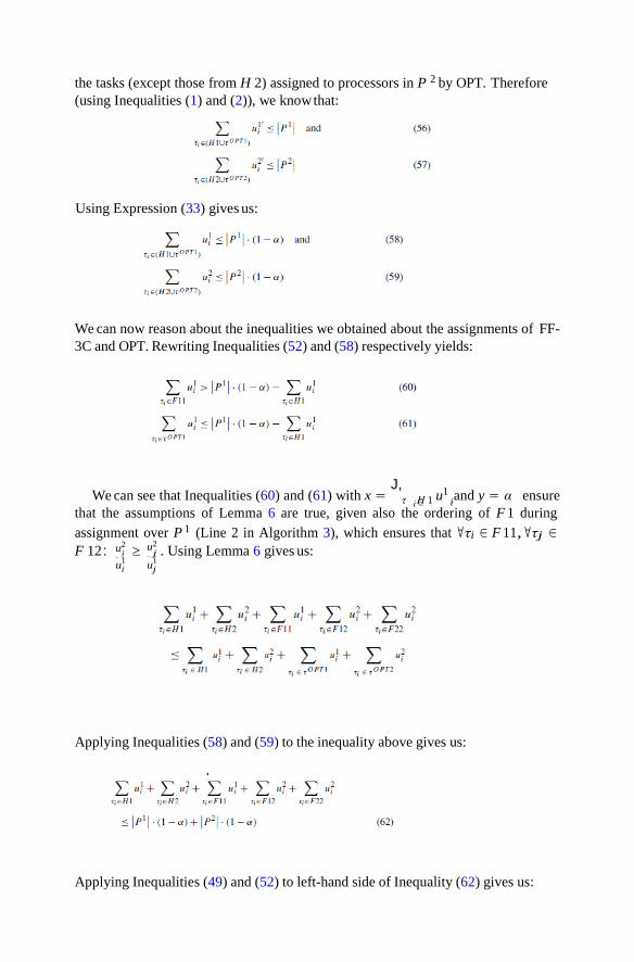
the tasks (except those from H 2) assigned to processors in P 2 by OPT. Therefore

(using Inequalities (1) and (2)), we know that:

Using Expression (33) gives us:

We can now reason about the inequalities we obtained about the assignments of FF-

3C and OPT. Rewriting Inequalities (52) and (58) respectively yields:

We can see that Inequalities (60) and (61) with x = J,

τ H 1 u1 and y = α ensure

that the assumptions of Lemma 6 are true, given also the ordering of F 1 during

assignment over P 1 (Line 2 in Algorithm 3), which ensures that ∀τi ∈ F 11, ∀τj ∈ u2 u2

F 12 : ≥ . Using Lemma 6 gives us: 1 1 i j

Applying Inequalities (58) and (59) to the inequality above gives us:

1

Applying Inequalities (49) and (52) to left-hand side of Inequality (62) gives us:

u

<

This is a contradiction.

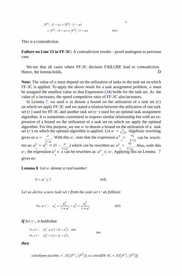
Failure on Line 23 in FF-3C: A contradiction results—proof analogous to previous

case.

We see that all cases where FF-3C declares FAILURE lead to contradiction.

Hence, the lemma holds. D

Note: The value of α must depend on the utilization of tasks in the task set on which

FF-3C is applied. To apply the above result for a task assignment problem, α must

be assigned the smallest value so that Expression (34) holds for the task set. As the

value of α increases, the speed competitive ratio of FF-3C also increases.

In Lemma 7, we used α to denote a bound on the utilization of a task set (τ )

on which we apply FF-3C and we stated a relation between the utilization of one task

set (τ ) used for FF-3C and another task set (τ ,) used for an optimal task assignment

algorithm. It is sometimes convenient to express similar relationship but with an ex-

pression of a bound on the utilization of a task set on which we apply the optimal

algorithm. For this purpose, we use α, to denote a bound on the utilization of a task set (τ ,) on which the optimal algorithm is applied. Let α, = 1

αα . Algebraic rewriting

− 1

gives us α = α, . With this α,, note that the expression u1,

= ui

can be rewrit- 1+α, i 1−α

1,

ten as: u1 = u1, × (1 − α,

) which can be rewritten as: u1 = ui

. Also, with this i i 1+α, i 1+α,

α,, the expression u1 ≤ α can be rewritten as: u1, ≤ α,. Applying this on Lemma 7

i i

gives us:

Lemma 8 Let α, denote a real number:

Let us derive a new task set τ from the task set τ , as follows:

If for τ ,, it holds that:

then

Proof The proof follows from the discussion above. D

The above result can also be expressed in terms of the additional processor speed

required by FF-3C as compared to that of an optimal algorithm for scheduling a given

task set.

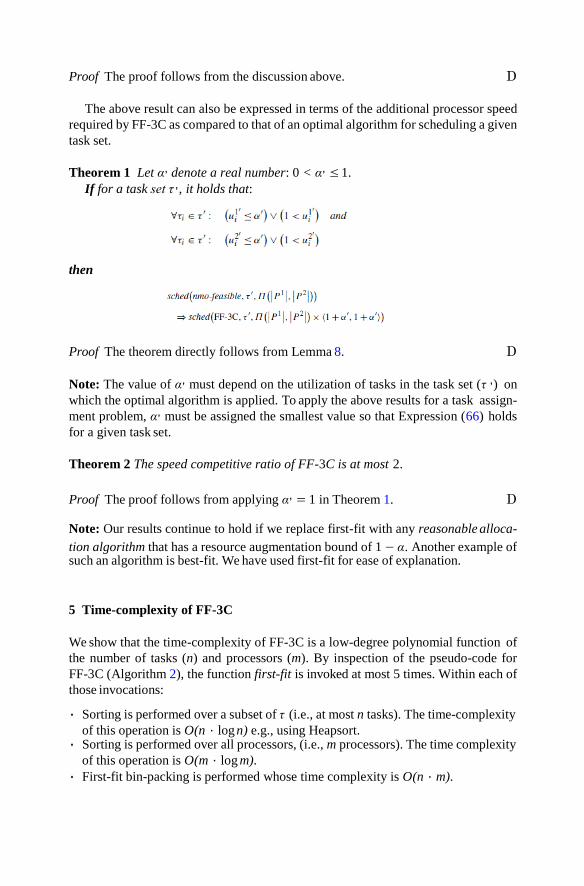
Theorem 1 Let α, denote a real number: 0 < α, ≤ 1.

If for a task set τ ,, it holds that:

then

Proof The theorem directly follows from Lemma 8. D

Note: The value of α, must depend on the utilization of tasks in the task set (τ ,) on

which the optimal algorithm is applied. To apply the above results for a task assign-

ment problem, α, must be assigned the smallest value so that Expression (66) holds

for a given task set.

Theorem 2 The speed competitive ratio of FF-3C is at most 2.

Proof The proof follows from applying α, = 1 in Theorem 1. D

Note: Our results continue to hold if we replace first-fit with any reasonable alloca-

tion algorithm that has a resource augmentation bound of 1 − α. Another example of such an algorithm is best-fit. We have used first-fit for ease of explanation.

5 Time-complexity of FF-3C

We show that the time-complexity of FF-3C is a low-degree polynomial function of

the number of tasks (n) and processors (m). By inspection of the pseudo-code for

FF-3C (Algorithm 2), the function first-fit is invoked at most 5 times. Within each of

those invocations:

• Sorting is performed over a subset of τ (i.e., at most n tasks). The time-complexity

of this operation is O(n · log n) e.g., using Heapsort. • Sorting is performed over all processors, (i.e., m processors). The time complexity

of this operation is O(m · log m).

• First-fit bin-packing is performed whose time complexity is O(n · m).

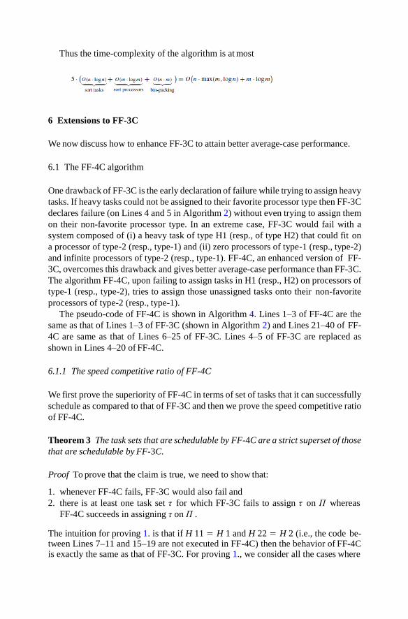
Thus the time-complexity of the algorithm is at most

6 Extensions to FF-3C

We now discuss how to enhance FF-3C to attain better average-case performance.

6.1 The FF-4C algorithm

One drawback of FF-3C is the early declaration of failure while trying to assign heavy

tasks. If heavy tasks could not be assigned to their favorite processor type then FF-3C

declares failure (on Lines 4 and 5 in Algorithm 2) without even trying to assign them

on their non-favorite processor type. In an extreme case, FF-3C would fail with a

system composed of (i) a heavy task of type H1 (resp., of type H2) that could fit on

a processor of type-2 (resp., type-1) and (ii) zero processors of type-1 (resp., type-2)

and infinite processors of type-2 (resp., type-1). FF-4C, an enhanced version of FF-

3C, overcomes this drawback and gives better average-case performance than FF-3C.

The algorithm FF-4C, upon failing to assign tasks in H1 (resp., H2) on processors of

type-1 (resp., type-2), tries to assign those unassigned tasks onto their non-favorite

processors of type-2 (resp., type-1).

The pseudo-code of FF-4C is shown in Algorithm 4. Lines 1–3 of FF-4C are the

same as that of Lines 1–3 of FF-3C (shown in Algorithm 2) and Lines 21–40 of FF-

4C are same as that of Lines 6–25 of FF-3C. Lines 4–5 of FF-3C are replaced as

shown in Lines 4–20 of FF-4C.

6.1.1 The speed competitive ratio of FF-4C

We first prove the superiority of FF-4C in terms of set of tasks that it can successfully

schedule as compared to that of FF-3C and then we prove the speed competitive ratio

of FF-4C.

Theorem 3 The task sets that are schedulable by FF-4C are a strict superset of those

that are schedulable by FF-3C.

Proof To prove that the claim is true, we need to show that:

1. whenever FF-4C fails, FF-3C would also fail and

2. there is at least one task set τ for which FF-3C fails to assign τ on Π whereas

FF-4C succeeds in assigning τ on Π .

The intuition for proving 1. is that if H 11 = H 1 and H 22 = H 2 (i.e., the code be- tween Lines 7–11 and 15–19 are not executed in FF-4C) then the behavior of FF-4C is exactly the same as that of FF-3C. For proving 1., we consider all the cases where

FF-4C declares FAILURE and show that FF-3C will also declare FAILURE in each

of those cases.

Failure on Line 10 in FF-4C: This implies that FF-4C could not assign all the tasks

in H 1 to their favorite processor type P 1 and hence only few tasks (H 11) were

assigned to P 1 and the rest were attempted to be assigned to their non-favorite pro-

2

cessors P 2 and failed. In such a case, FF-3C would have declared failure on Line 4

(in Algorithm 2) itself as it would also fail to assign all the tasks in H 1 to P 1 since it

also uses the same first-fit algorithm (of Algorithm 3) that is used by FF-4C.

Failure on Line 18 in FF-4C: When the algorithm fails here, there are two scenarios

that need to be considered with respect to the assignment of tasks in H 1 (earlier in

the algorithm): (i) all the tasks in H 1 were successfully assigned to P 1 (indicated

by boolH 1 = FALSE, i.e., Lines 7–11 were not executed at all) and (ii) only few tasks from H 1 could be assigned to P 1 and hence the rest were assigned to P 2

(indicated by boolH 1 = TRUE). For the first scenario, the proof is symmetric to the previous case (i.e., proof given for ‘Failure on Line 10 in FF-4C’; FF-3C would have

declared FAILURE on Line 5 itself as it would also fail to assign all the tasks in H 2

to processors in P 2). For the second scenario, the proof is analogous to the previous case as FF-3C would have declared FAILURE on Line 4 (in Algorithm 2) itself as

soon as a task from H1 was failed to be assigned to P 1.

Failure on Lines 24, 30 and 38 in FF-4C: When the algorithm fails on one of these lines, our proof depends on the assignment of tasks in H 1 (resp., H 2) earlier in the algorithm, i.e., whether all the tasks of H 1 (resp., H 2) have been successfully as-

signed to their favorite processors, i.e., P 1 (resp., P 2) or only few tasks could be assigned to their favorite processors and the rest to the non-favorite processors, i.e.,

H 11 on P 1 and H 12 on P 2 (resp., H 22 on P 2 and H 21 on P 1). In the algorithms, this information is captured using a boolean variable, boolH 1 (resp., boolH 2). For

example, boolH 1 = FALSE indicates that all the tasks of H 1 were assigned on their favorite processors P 1 and boolH 1 = TRUE implies that only few tasks from H 1, i.e., H 11 could be assigned on their favorite processors P 1 and the rest, i.e., H 12,

were assigned on their non-favorite processors P 2. Analogous explanation holds for

boolean variable boolH 2. Hence, with the help of these two boolean variables we

have captured all the possible scenarios for FF-4C to fail (on one of the Lines 24,

30 or 38) in Table 2 along with the corresponding proof to look for in the paper

(as the proofs provided earlier in the paper can be reused to reason about these sce-

narios).

For proving 2., we illustrate the superiority of FF-4C over FF-3C with an example

task set. D

Example 3 Consider a platform comprising a processor P1 of type-1 and a processor

P2 of type-2, a task set τ = {τ1, τ2, τ3} shown in Table 3. It is trivial to observe that a schedulable assignment exists for this task set on the

given platform: assign τ1 and τ3 to P1 and τ2 to P2. We now simulate the behavior

of FF-4C and FF-3C for this task set on the given platform and show that FF-4C

succeeds whereas FF-3C fails.

First, let us look at FF-4C. On Line 1 (see Algorithm 4), FF-4C groups the tasks

as follows: H 1 = {τ1, τ2} and F 1 = {τ3}. On Line 5, FF-4C calls first-fit sub-routine to assign tasks in H 1 to processor P1

of type-1. The sub-routine succeeds in assigning task τ1 to P1 and fails to assign the other task τ2 to P1 as there is not enough capacity left on P1. Hence, after executing

Line 5 of FF-4C, we have: H 11 = {τ1}. After assigning τ1 to P1, the remaining

utilization on P1 is 1 − E.

τ1 1

τ2 1

τ3 1

1

1

1

2

Table 2 Summary of proof of speed competitive ratio of FF-4C for different cases

boolH1 boolH2 Explanation of the scenario Use the reasoning of

FALSE FALSE All the tasks of H 1 and H 2 were assigned to their favorite

processors P 1 and P 2 respectively. This indicates that

the behavior of FF-4C is same as that of FF-3C in this

case (i.e., code on Lines 7–11 and 15–19 of FF-4C is not executed). Hence, the reason for failure of FF-4C on Line

24, 30 and 38 is same as that of failure of FF-3C on Line

9, 15 and 23

FALSE TRUE Only few tasks of H 2 (H 22) could be assigned on P 2 and

the rest (H 21) were assigned to P 1. In such a case, FF-3C would have failed on Line 5 itself during the assignment

of H 2 on P 2 as it fails to assign all the tasks from H 2 on

P 2 and does not even try to assign the failed tasks of H 2

on P 1

TRUE FALSE This case is analogous to the previous case where only

few tasks of H 1 (H 11) could be assigned to P 1 and rest

(H 12) were assigned to P 2. In this case, FF-3C would

have failed on Line 4 itself during the assignment of H 1

on P 1 as it fails to assign all the tasks from H 1 on P 1 and

does not even try to assign the failed tasks of H 1 on P 2

TRUE TRUE This case is similar to one of the two previous cases,

i.e., boolH1 = FALSE ∧ boolH2 = TRUE and boolH1 =

TRUE ∧ boolH2 = FALSE

Proof of Lemma 7,

‘Failure on Line 9, 15

and 23’ respectively

Proof of Theorem 3,

‘Failure on Line 18 in

FF-4C’

Proof of Theorem 3,

‘Failure on Line 10 in

FF-4C’

Proof of Theorem 3,

‘Failure on Line 10

in FF-4C’ and ‘Failure

on Line 18 in FF-4C’

respectively

Table 3 An example task set

schedulable by FF-4C but not

by FF-3C

τi u1 2

i ui belongs to

2 + E

2 + E

2 − E

2 + 2E H1

2 + 2E H1

2 F1

On Line 8, it creates H 12 = {τ2}. On Line 9, it successfully assigns τ2 to processor P2 using first-fit sub-routine.

After assigning τ2 to processor P2; the remaining utilization on P2 is 1 − 2E.

On Line 21, it successfully assigns τ3 (of F 1) to processor P1 using first-fit sub-

routine. After assigning τ3 to P1, the remaining utilization on P1 is 0.

So, the final assignment of tasks is as follows: τ1 and τ3 are assigned to P1 and τ2

is assigned to P2—hence, FF-4C succeeds.

Now let us look at FF-3C. FF-3C groups the tasks as follows: H 1 = {τ1, τ2} and

F 1 = {τ3}. FF-3C fails to assign both the tasks in H 1 to processor P1 of type-1 since

the sum of their utilization (( 1 + E) + ( 1 + E) = 1 + 2E) exceeds 1.0. 2 2

Hence FF-3C declares FAILURE on Line 4 (see Algorithm 2).

2

Thus, we showed that: 1. whenever FF-4C fails, FF-3C also fails and 2. there is at

least one task set τ for which FF-3C fails to assign τ on Π whereas FF-4C succeeds

in assigning τ on Π . Hence the theorem holds. D

Now we prove the speed competitive ratio of FF-4C.

Lemma 9 Let α denote a real number: 0 <α ≤ 1 .

Let us derive a new task set τ , from the task set τ as follows:

then

Proof We know from Lemma 7 that

Also, from Theorem 3 we know that if FF-3C succeeds to assign a task set τ on a

computing platform Π (|P 1|, |P 2|) then FF-4C succeeds as well (on the same plat- form). Formally, this can be stated as:

Combining Expression (67) and (68) gives us:

Hence, the proof. D

Similar to Lemma 7, the above lemma uses α to denote a bound on the utilization

of a task set (τ ) on which we apply FF-4C and states a relation between the utilization

of one task set (τ ) used for FF-4C and another task set (τ ,) used for an optimal task

assignment algorithm. Now, similar to Lemma 8, let us express this relationship with

α,, an expression of a bound on the utilization of a task set (τ ,) on which we apply

the optimal algorithm.

Lemma 10 Let α, denote a real number: 0 < α, ≤ 1.

Let us derive a new task set τ from the task set τ , as follows:

If for τ ,, it holds that:

then

Proof The reasoning is analogous to the proof of Lemma 8. D

Now, we express the above result in terms of the additional processor speed re-

quired by FF-4C as compared to that of an optimal algorithm for scheduling a given

task set.

Theorem 4 Let α, denote a real number 0 < α, ≤ 1.

If for a task set τ ,, it holds that:

then

Proof The theorem directly follows from Lemma 10. D

Theorem 5 The speed competitive ratio of FF-4C is at most 2.

Proof The proof follows from applying α, = 1 in Theorem 4. D

6.1.2 Time-complexity of FF-4C

We can use the same reasoning provided for the time-complexity of FF-3C in Sect. 5 for FF-4C as well. FF-4C uses the first-fit sub-routine at most seven times (see Al- gorithm 4) and each time (i) sorting is performed over at most n tasks whose com-

plexity is O(n · log n) (ii) sorting is performed over m processors whose complexity is O(m · log m) and (iii) first-fit bin-packing takes O(n · m) time. Hence, the time-

complexity of FF-4C is: O(n · max(m, log n) + m · log m).

6.2 The FF-4C-NTC algorithm

In FF-3C (and also in FF-4C), tasks are categorized as H 1, F 1, H 2 and F 2 and this

makes it possible to prove the speed competitive ratio the way we do it. Unfortunately,

this categorization can misguide the algorithm to assign a task in a way which causes

1

a failure later on. For example, consider a task set with two tasks τ1 with u1 = 0.5, u2 1 2

1 = 1.0 and τ2 with u2 = 1.0, u2 = 1.0 + E and a platform comprising a processor P1 of type-1 and P2 of type-2. Clearly, there exists a schedulable assignment of the given task set on the given platform: assign τ1 to P2 and τ2 to P1. Now let us see

what FF-3C does for this problem instance. FF-3C classifies τ1 and τ2 as H 1 and

assigns τ1 to P 1 and then tries to assign τ2 to P 1 but fails. FF-4C also exhibits

similar behavior: it assigns τ1 to P 1 and then it attempts to assign τ2 to P 2 after

an unsuccessful attempt to assign it to P 1 and fails. Hence, both FF-3C and FF-4C fails on this task set. Therefore, we present a new algorithm namely, FF-4C-NTC to

handle such cases.

The algorithm FF-4C-NTC classifies tasks as τ 1 and τ 2 as defined by Inequali-

ties (4) and (5), and for each class, assigns tasks in order of decreasing u2/u1 for i i type-1 processors and decreasing u1/u2 for type-2 processors, respectively with ties

i i

broken favoring the task with lower identifier. FF-4C-NTC does not classify τ 1 into

H 1 and F 1 nor τ 2 into H 2 and F 2 (as was the case with FF-3C and FF-4C): It only considers favorite/non-favorite processor types and disregards the information (used by both FF-3C and FF-4C) whether a task is heavy or not. The pseudo-code of FF-

4C-NTC is shown in Algorithm 5. The algorithm first tries to assign tasks from τ 1

on their favorite processors of type P 1 using first-fit and if any of these tasks could

not be assigned then it tries to assign them on their non-favorite processor type P 2—

and analogously for τ 2. For the above example, FF-4C-NTC assigns τ1 to P2 and τ2

to P1.

FF-4C-NTC also has the same time-complexity of O(n · max(m, log n)+m · log m) as the previously discussed algorithms.

This algorithm will be used as a sub-routine in our next algorithm, namely FF-

4C-COMB, discussed in Sect. 6.3. We will not use FF-4C-NTC as a stand-alone

algorithm and hence we will not discuss its speed competitive ratio.

2

6.3 The FF-4C-COMB algorithm

As discussed in earlier sections, for some task sets FF-4C succeeds whereas FF-4C-

NTC fails and for other task sets FF-4C-NTC succeeds whereas FF-4C fails. FF-4C-

COMB exploits this fact by making use of both the algorithms to get the best out of

the two—pseudo-code is listed in Algorithm 6. It first attempts to assign the task set

with FF-4C and, upon failing, it tries with FF-4C-NTC.

6.3.1 The speed competitive ratio of FF-4C-COMB

In this section, we establish the speed competitive ratio of FF-4C-COMB.

Lemma 11 Let α denote a real number: 0 <α ≤ 1 .

Let us derive a new task set τ , from the task set τ as follows:

If for τ , it holds that:

then

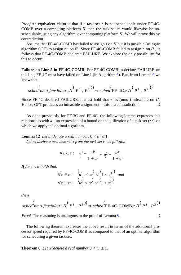
Proof An equivalent claim is that if a task set τ is not schedulable under FF-4C-

COMB over a computing platform Π then the task set τ , would likewise be un-

schedulable, using any algorithm, over computing platform Π . We will prove this by

contradiction.

Assume that FF-4C-COMB has failed to assign τ on Π but it is possible (using an

algorithm OPT) to assign τ , on Π . Since FF-4C-COMB failed to assign τ on Π , it

follows that FF-4C-COMB declared FAILURE. We explore the only possibility for

this to occur:

Failure on Line 5 in FF-4C-COMB: For FF-4C-COMB to declare FAILURE on

this line, FF-4C must have failed on Line 1 (in Algorithm 6). But, from Lemma 9 we

know that

sched(nmo-feasible,τ ,,Π

( P 1 , P 2

)) ⇒ sched

(FF-4C,τ,Π

( P 1 , P 2

))

Since FF-4C declared FAILURE, it must hold that τ , is (nmo-) infeasible on Π .

Hence, OPT produces an infeasible assignment—this is a contradiction. D

As done previously for FF-3C and FF-4C, the following lemma expresses this

relationship with α,, an expression of a bound on the utilization of a task set (τ ,) on

which we apply the optimal algorithm.

Lemma 12 Let α, denote a real number: 0 < α, ≤ 1.

Let us derive a new task set τ from the task set τ , as follows:

u1, ∀τi ∈ τ , : u1 = i

u2,

∧ u2 = i

If for τ ,, it holds that:

i 1 + α,

i 1 + α,

∀τi ∈ τ , : (u1,

≤ α,)

∨ (1 < u1, )

and i i

∀τi ∈ τ , : (u2,

≤ α,)

∨ (1 < u2, )

i i

then

sched(nmo-feasible,τ ,,Π

( P 1 , P 2

)) ⇒ sched

(FF-4C-COMB,τ,Π

( P 1 , P 2

))

Proof The reasoning is analogous to the proof of Lemma 8. D

The following theorem expresses the above result in terms of the additional pro-

cessor speed required by FF-4C-COMB as compared to that of an optimal algorithm

for scheduling a given task set.

Theorem 6 Let α, denote a real number 0 < α, ≤ 1.

If for a task set τ ,, it holds that:

then

Proof The theorem directly follows from Lemma 12. D

Theorem 7 The speed competitive ratio of FF-4C-COMB is at most 2.

Proof The proof follows from applying α, = 1 in Theorem 6. D

6.3.2 Time-complexity of FF-4C-COMB

We know that both FF-4C and FF-4C-NTC have the same time-complexity of O(n ·

max(m, log n) + m · log m). FF-4C-COMB (pseudo-code in Algorithm 5) calls FF-4C first and upon failing it calls FF-4C-NTC. Hence, time-complexity of FF-4C-COMB

is also O(n · max(m, log n) + m · log m).

7 Experimental setup and results

After seeing the theoretical bounds of our algorithms, we wanted to evaluate their

performance and compare it with state-of-the-art. For this purpose, we looked at the

following issues: (i) how well our algorithms perform compared to state-of-the-art in

successfully assigning the tasks to processors, i.e., how much faster processors our

algorithms need in order to assign a task set compared to state-of-the-art algorithms?,

(ii) how fast our algorithms run compared to state-of-the-art algorithms? and (iii) how

much pessimism is there in our theoretically derived performance bounds?

In order to answer these questions, we performed two sets of experiments. First,

we compared the performance of our algorithms with two state-of-the-art algorithms

(Baruah 2004b, 2004c). Both Baruah (2004b, 2004c) proposed solutions with speed

competitive ratio of 2. Hence, we evaluated the performance of our algorithms with

Baruah (2004b, 2004c) by setting α, = 1 when their speed competitive ratio becomes 2 as well. We observed that, in our experiments with randomly generated task sets,

our algorithms perform better in practice than state-of-the-art. We also observed that

our algorithms run significantly faster compared to state-of-the-art. Then, we simu-

lated our algorithms for different values of α,. We observed that even for this im-

proved analysis case (where the speed competitive ratio is quantified with task set

parameters as opposed to a constant number (Andersson et al. 2010)), they still per-

form better than indicated by the speed competitive ratio. We now discuss both the

cases in detail.

OP T

− i x

7.1 Comparison with state-of-the-art

We implemented two versions of Baruah (2004c) (SKB-RTAS and SKB-RTAS-IMP)

and two versions of Baruah (2004b) (SKB-ICPP and SKB-ICPP-IMP). SKB-RTAS

and SKB-ICPP follow from the corresponding papers; the -IMP variants are our

improved versions of the respective algorithms (see description below). We imple-

mented all algorithms using C on Windows XP on an Intel Core2 (2.80 GHz) ma-

chine. For SKB-algorithms we also used a state-of-art LP/ILP solver, IBM ILOG

CPLEX (IBM Inc. 2011).

In Baruah (2004c), a two step algorithm to assign tasks on a heterogeneous plat-

form is proposed. The algorithm is as follows:

1. The assignment problem is formulated as ILP and then relaxed to LP. The LP

formulation is solved using an LP solver. Tasks are then assigned to the processors

according to the values of the respective indicator variables in the solution. Using

certain tricks (Potts 1985), it is shown that there exists a solution (for example,

the solution that lies on the vertex of the feasible region) to the LP formulation in

which all but at most m − 1 tasks are integrally assigned to processors where m is the number of processors.

2. The remaining at most m − 1 tasks are integrally assigned on the remaining ca- pacity of the processors using “exhaustive enumeration”.

While assigning the remaining tasks in Step 2, the author illustrates with an example

that the utilization of the task under consideration is compared against the value 1 − z for assignment decisions on any processor, where z (returned by the LP solver) is the maximum utilized fraction of any processor—SKB-RTAS implements this (pes-

simistic) rule. Since the actual remaining capacity of each processor6 can easily be

computed from the LP solver solution, SKB-RTAS-IMP uses that, instead of 1 − z, to test assignments, for improved average-case performance.

In Baruah (2004b), author proposes a two step algorithm, namely taskPartition, to

assign tasks on a heterogeneous platform. The algorithm is as follows:

1. This step is similar to Step 1 of (Baruah 2004c) as described above.

2. The remaining at most m − 1 tasks are assigned using the bipartite matching tech-

nique such that at most one task from the m − 1 remaining tasks is assigned to each processor.

Let r1, r2,..., rk denote the distinct utilization values in the given task set sorted in

the increasing order, where 1 ≤ k ≤ m × n. The two step algorithm is called repeat-

edly by a procedure, namely optSrch, with different values of ri , 1 ≤ i ≤ k. When taskPartition is called by optSrch with a ri , all the utilizations that are greater than

ri are set to infinity. The procedure optSrch checks for the condition Uri

≤ 1 − ri

6The actual remaining capacity on processor p is 1 J,

: i,p = 1 ui,p where ui,p represents the utilization

of τi on processor p (Baruah 2004c). The symbol xi,p represents the indicator variable and the value

of 0 ≤ xi,p ≤ 1 indicates how much fraction of task τi must be assigned to processor p. The term 1 − J,

i:xi,p =1 ui,p gives an accurate estimation of the remaining capacity on processor p as it ignores the fractionally assigned tasks on that processor whereas z is pessimistic since it includes those tasks as well.

OP T

z

in order to determine whether a feasible mapping has been obtained by taskPartition

where Uri

denotes the value of objective function of the vertex solution returned

by LP solver—SKB-ICPP implements this feasibility test. This pessimistic condition

severely impacts performance. Hence, SKB-ICPP-IMP implements a better feasibil-

ity condition which checks that the sum of utilizations of all the tasks assigned to each

processor does not exceed its computing capacity thereby improving its performance

significantly in practice.

The necessary multiplication factor is defined as the amount of extra speed of pro-

cessors the algorithm needs, for a given task set, so as to succeed, as compared to

an optimal task assignment algorithm. We assess (i) the average-case performance of

algorithms by creating a histogram of necessary multiplication factor and also (ii) the

average run-time of each algorithm. Since all the SKB-algorithms use CPLEX, an

external program, for assigning tasks to processors (for solving LP), they are penal-

ized by the startup time and reading of the problem instance from an input file—we

refer to this overhead as CPLEX overhead. We deal with this issue by measuring the

average time for CPLEX overhead and subtract it from the measured running time of

those algorithms that rely on CPLEX. In particular, SKB-ICPP and SKB-ICPP-IMP

invoke CPLEX multiple times for a single task set. So, we record, for such algorithms

for each task set how many times CPLEX was invoked and subtract as many times

the average CPLEX overhead.

We have considered the following as CPLEX overhead: (i) starting CPLEX from

our program through a system call and (ii) reading of an input file (i.e., problem in-

stance) by CPLEX. We measured the total time that CPLEX takes to start and read

the largest input file possible for our simulation (i.e., problem involving 12 tasks and

6 processors). We measured this time for 200 iterations (same as the number of task

sets for which we have computed the average execution times) and took the average

of these measurements. This average value was subtracted (i) once for every measure-

ment of SKB-RTAS and SKB-RTAS-IMP and (ii) r times for every measurement of

SKB-ICPP and SKB-ICPP-IMP where r is the number of different ui,j values the

algorithm tries for each task set.

The problem instances (number of tasks, their utilizations and number of proces-

sors of each type) were generated randomly. Each problem instance had at most 12

tasks and at most 3 processors of each type. We term a task set critically feasible if it

is feasible on a given heterogeneous multiprocessor platform but rendered infeasible if u1 and u2 of all the tasks in the system are increased by an arbitrarily small factor.

i i

To obtain critically feasible task sets from randomly generated task sets, we perform

the assignment with ILP as discussed in Baruah (2004b) and obtain z—the utilization of the most utilized processor, and then multiply all the task utilizations by a factor

of 1 and repeatedly feed back to CPLEX till 0.98 <z ≤ 1. We ran each algorithm on 15000 critically feasible task sets to obtain the necessary

multiplication factor. The pseudo-code for determining the necessary multiplication

factor for task sets is shown in Algorithm 7. We input a task set to algorithm A (where

A can be: FF-3C, FF-4C, FF-4C-NTC, FF-4C-COMB, SKB-RTAS, SKB-RTAS-IMP,

SKB-ICPP or SKB-ICPP-IMP) and if the algorithm cannot find a feasible mapping,

we increment the multiplication factor by a small step, i.e., STEP = 0.01 and divide

the original u1 and u2 of each task by the new multiplication factor (whose value is i i

mult_fact

Algorithm 7: Pseudo-code to determine necessary multiplication factor for an

algorithm

1 STEP := 0.01

2 for i = 1 to 15000 do //for each critically feasible task set 3 found_mult_fact := false

4 mult_fact := 1 5 Let curr_τ denote the critically feasible task set under consideration

6 while (found_mult_factor /= true) do

7 Multiply the utilizations of all the tasks in curr_τ by a factor of 1.0 ; let temp_τ

8

9

10

11

12

13

14

15

16 end

end

denote the resulting task set

result := mappingAlgo(temp_τ , assign_info) // assign_info is an output

variable which contains the task assignment information

if (result = SUCCESS) then

found_mult_fact := true print mult_fact, assign_info

else

mult_fact := mult_fact + STEP end

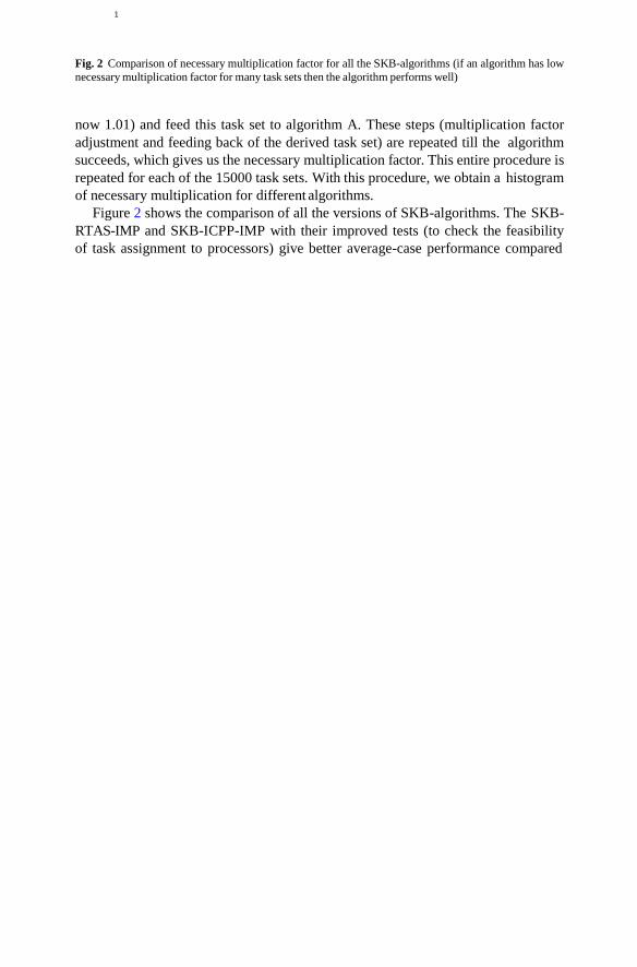
Fig. 2 Comparison of necessary multiplication factor for all the SKB-algorithms (if an algorithm has low

necessary multiplication factor for many task sets then the algorithm performs well)

now 1.01) and feed this task set to algorithm A. These steps (multiplication factor

adjustment and feeding back of the derived task set) are repeated till the algorithm

succeeds, which gives us the necessary multiplication factor. This entire procedure is

repeated for each of the 15000 task sets. With this procedure, we obtain a histogram

of necessary multiplication for different algorithms.

Figure 2 shows the comparison of all the versions of SKB-algorithms. The SKB-

RTAS-IMP and SKB-ICPP-IMP with their improved tests (to check the feasibility

of task assignment to processors) give better average-case performance compared

Fig. 3 Comparison of necessary multiplication factor for all of our FF-algorithms (if an algorithm has

low necessary multiplication factor for many task sets then the algorithm performs well)

Fig. 4 Comparison of necessary multiplication factor for three algorithms (if an algorithm has low nec-

essary multiplication factor for many task sets then the algorithm performs well)

to their counterparts. As we can see, SKB-RTAS-IMP gives the best performance

among all the SKB-algorithms.

Figure 3 shows the performance of all our FF-algorithms. As we can see, FF-

3C performs poorly compared to the other three, and FF-4C-COMB gives the best

performance among all the FF-algorithms as it makes use of both FF-4C and FF-4C-

NTC algorithms (whose performance lies between FF-3C and FF-4C-COMB).

Since SKB-RTAS-IMP offered the best necessary multiplication factor among all

the SKB-algorithms and FF-4C-COMB offered the best necessary multiplication fac-

tor among all the FF-algorithms, we only depict these along with FF-3C since it is

the baseline of all our algorithms in Fig. 4. As seen in our experiments, the neces-

sary multiplication factor of FF-4C-COMB never exceeded 1.35 whereas for FF-3C

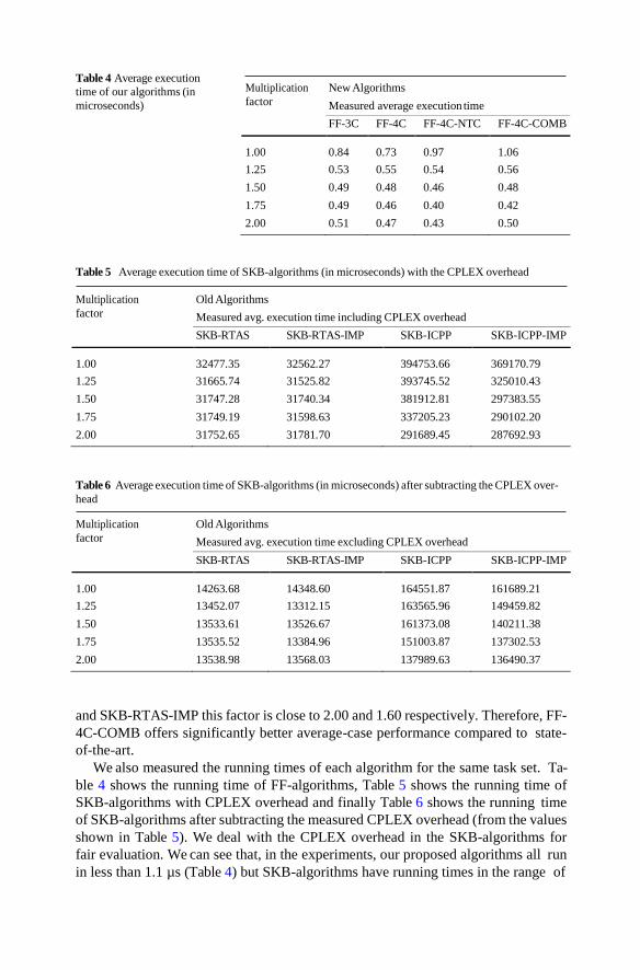
Table 4 Average execution

time of our algorithms (in

microseconds)

Multiplication

factor

New Algorithms

Measured average execution time

FF-3C FF-4C FF-4C-NTC FF-4C-COMB

1.00 0.84 0.73 0.97 1.06

1.25 0.53 0.55 0.54 0.56

1.50 0.49 0.48 0.46 0.48

1.75 0.49 0.46 0.40 0.42

2.00 0.51 0.47 0.43 0.50

Table 5 Average execution time of SKB-algorithms (in microseconds) with the CPLEX overhead

Multiplication

factor

Old Algorithms

Measured avg. execution time including CPLEX overhead

SKB-RTAS SKB-RTAS-IMP SKB-ICPP SKB-ICPP-IMP

1.00 32477.35 32562.27 394753.66 369170.79

1.25 31665.74 31525.82 393745.52 325010.43

1.50 31747.28 31740.34 381912.81 297383.55

1.75 31749.19 31598.63 337205.23 290102.20

2.00 31752.65 31781.70 291689.45 287692.93

Table 6 Average execution time of SKB-algorithms (in microseconds) after subtracting the CPLEX over-

head

Multiplication

factor

Old Algorithms

Measured avg. execution time excluding CPLEX overhead

SKB-RTAS SKB-RTAS-IMP SKB-ICPP SKB-ICPP-IMP

1.00 14263.68 14348.60 164551.87 161689.21

1.25 13452.07 13312.15 163565.96 149459.82

1.50 13533.61 13526.67 161373.08 140211.38

1.75 13535.52 13384.96 151003.87 137302.53

2.00 13538.98 13568.03 137989.63 136490.37

and SKB-RTAS-IMP this factor is close to 2.00 and 1.60 respectively. Therefore, FF-

4C-COMB offers significantly better average-case performance compared to state-

of-the-art.

We also measured the running times of each algorithm for the same task set. Ta-

ble 4 shows the running time of FF-algorithms, Table 5 shows the running time of

SKB-algorithms with CPLEX overhead and finally Table 6 shows the running time

of SKB-algorithms after subtracting the measured CPLEX overhead (from the values

shown in Table 5). We deal with the CPLEX overhead in the SKB-algorithms for

fair evaluation. We can see that, in the experiments, our proposed algorithms all run

in less than 1.1 µs (Table 4) but SKB-algorithms have running times in the range of

13500 to 160000 µs (Table 6). Hence all of our algorithms run at least 12000 times

faster.

7.2 Evaluation of our algorithms for different values of α,

We evaluated the performance of our algorithms for different values of α,. We ran- domly generated 100000 critically feasible task sets. Each critically feasible task set

had at most 25 tasks and at most 2 processors of each type.7 We then classified the

critically feasible task sets based on the value of α, of each task set into ten groups—

for a given critically feasible task set, if α, ≤ 0.1 then the task set belongs to the first

group, if 0.1 < α, ≤ 0.2 then the task set belongs to the second group, . . . , and finally

if 0.9 < α, ≤ 1.0 then the task set belongs to the tenth group. Then, we ran each al- gorithm, i.e., FF-3C, FF-4C, FF-4C-NTC and FF-4C-COMB for the above generated

critically feasible task sets and observed their necessary multiplication factors. We

plotted the histogram of necessary multiplication factors for each of these algorithms

for task sets in each of the groups. Since the experiments in previous subsection have

confirmed that FF-4C-COMB performs better compared to all other algorithms and

since FF-3C is the baseline of all our algorithms, we only depict these.

Figure 5 shows the performance of FF-3C and FF-4C-COMB algorithms. We

only show the results obtained for five cases, i.e., 0.1 < α, ≤ 0.2, 0.3 < α, ≤ 0.4,

. . . , 0.9 < α, ≤ 1.0. The observations for other cases follow the same trend. As we can see from the graphs, for the vast majority of task sets, the algorithms perform

much better than indicated by their speed competitive ratio, even when we consider

the speed competitive ratio as a function of task set parameters.

8 Clustered scheduling

Having seen the excellent performance of FF-3C—both its performance bound and

its performance in experimental evaluation—we now consider a heterogeneous mul-

tiprocessor platform where processors have two types (just like before) but processors

of each type are organized into clusters of processors. Such a problem has been stud-

ied in the past in the context of identical multiprocessor platform (Qi et al. 2010).

However, to the best of our knowledge, no such work exists for heterogeneous plat-

forms with two types of processors. We define a cluster of processors as a subset of

all processors such that (i) all processors in the cluster are of the same type, (ii) each

cluster has equal number of processors and (iii) a task can migrate between proces-

sors in the same cluster. Note that a consequence of (ii) is that there is no “remain-

ing cluster” with fewer processors. Related to (iii), the assumption that migration is

allowed, we assume that an optimal migrative scheduling algorithm is used to sched-

7Since we only evaluate FF-algorithms in this batch of experiments and do not run SKB-algorithms which

make use of linear programming solvers thereby taking much longer to output the solution, we could

afford to set a higher bound on the number of tasks in each problem instance compared to previous set of

experiments.

k

k

2

Fig. 5 Performance of FF-3C and FF-4C-COMB algorithm in terms of necessary multiplication factors for different values of α, (if an algorithm has low necessary multiplication factor for many task sets then

the algorithm performs well)

ule the tasks in each cluster; the research literature offers several such algorithms

for implicit-deadline sporadic scheduling, for example, the class of Pfair schedul-

ing algorithms (Anderson and Srinivasan 2000), sporadic EKG with timeslot being

the greatest common divisor of minimum inter-arrival times (Andersson and Bletsas

2008) and the DP-WRAP framework (Levin et al. 2010).

For the purpose of discussing scheduling on such a platform, let k denote the

number of processors in a cluster. Clearly, we have |P 1|

clusters containing type-1

processors and we have |P 2|

clusters containing type-2 processors. Let α denote a

real number: 0 <α ≤ 1 . Let τ denote the task set such that:

k + k

– |P |

– |P |

j ∈ j

k + k

– |P |

– |P |

j

j

k + k

τ p

τ p

– |P |

– |P |

|P |

– |P |

k

k

k

k

∀τi ∈ τ : (u1 ≤ α

) ∨

(1 − α< u1

) and

i i

∀τi ∈ τ : (u2 ≤ α

) ∨

(1 − α< u2

)

i i

We want to schedule the task set τ on computing platform Π (with clusters as men-

tioned above) with migration allowed between processors in the same cluster. We

formulate this problem as follows:

Partition the set of tasks into |P 1|

|P 2|

partitions where

1

k of the partitions are said to be of type-1 2

k of the partitions are said to be of type-2 1

– for each type-1 partition p, it holds that: J,

τj ∈p uj ≤ k

– for each type-2 partition p, it holds that: J,

τ p u2 ≤ k

Once partitions have been formed, it is straightforward to assign tasks to processors (all tasks in a type-1 partition are assigned to a cluster of type-1 processor; analo-

gously for type-2). Let us consider the special case where it holds that τ = F 1 ∪ F 2. The partitioning problem described above can be rewritten as follows:

Partition the set of tasks into |P 1|

|P 2|

partitions where

1

k of the partitions are said to be of type-1 2

k of the partitions are said to be of type-2

– for each type-1 partition p, it holds that: J,

τj ∈p

u1

k ≤ 1

– for each type-2 partition p, it holds that: J,

τj ∈p

u2

k ≤ 1

Because of τ = F 1 ∪ F 2, we have that all tasks are “light”. Hence if the utilization of each task would be divided by k then all tasks would still be light. This, combined with Lemma 7, gives us that:

– If it is possible to partition the set of tasks into |P 1|

|P 2|

partitions where 1

k of the partitions are said to be of type-1 2

k of the partitions are said to be of type-2

– for each type-1 partition p, it holds that: J,

j ∈

– for each type-2 partition p, it holds that: J,

j ∈

1

j ≤ 1 2

j ≤ 1

– then FF-3C can be used to assign tasks to partitions (where a partition corresponds to a processor in FF-3C) and this outputs a partitioning of the set of tasks into |P 1|

k + – |P 1|

2

k partitions where

k of the partitions are said to be of type-1 2

k of the partitions are said to be of type-2 – for each type-1 partition p, it holds that:

J,

1 j 1

τj ∈p k ≤

1− α

– for each type-2 partition p, it holds that: J,

2 j 1

τj ∈p k ≤

1− α

u

u

u

u

1 2

Hence, we can see that FF-3C can be used to solve the problem of scheduling

implicit-deadline sporadic tasks on a heterogeneous multiprocessor with clustering.

Clearly, we do not have to use FF-3C; we can use any of its (average-case perfor-

mance) improved versions, i.e., FF-4C, FF-4C-NTC, FF-4C-COMB.

9 Discussion and conclusions

The heterogeneous multiprocessor computational model (i.e., unrelated parallel ma-

chines) is more general than identical or uniform multiprocessors, in terms of the sys-

tems that it can accommodate. Generally, this called for algorithms with large compu-

tational complexity, for provably good performance. We partially solve the issue via a

scheduling algorithm for multiprocessors consisting of two unrelated processor types.

This restricted model is of great practical interest, as it captures many current/future

single-chip heterogeneous multiprocessors (AMD Inc 2010; Gschwind et al. 2006;

Maeda et al. 2005; Freescale Semiconductor 2007). Our proposed algorithm, FF-3C,

is low-degree polynomial in time-complexity, i.e., faster than algorithms based on

ILP (or its relaxation to LP). We also proved that the speed competitive ratio of FF- 3C is 1

−α where 0 <α ≤ 1 .

Further, we designed variations of FF-3C which provide better average-case per-

formance and have the same time-complexity and the same speed competitive ratio

as that of FF-3C. We would like to mention that, in our experimental evaluations,

one of our new algorithms, FF-4C-COMB, runs 12000 to 160000 times faster and

has significantly smaller necessary multiplication factor than state-of-the-art algo-

rithms (Baruah 2004b, 2004c). We also presented a version of FF-3C targeted for

two-type heterogeneous multiprocessors where processors are organized into clus-

ters and where migration of tasks is allowed between processors of the same cluster.

Acknowledgements This work was partially supported by National Funds through FCT (Portuguese

Foundation for Science and Technology) and by ERDF (European Regional Development Fund)

through COMPETE (Operational Programme ‘Thematic Factors of Competitiveness’), within project

Ref. FCOMP-01-0124-FEDER-022701; by FCT and COMPETE (ERDF), within REHEAT project, ref.

FCOMP-01-0124-FEDER-010045; by FCT and ESF (European Social Fund) through POPH (Portuguese

Human Potential Operational Program), under PhD grant SFRH/BD/66771/2009.

References

AMD Inc (2010) AMD fusion family of APUs: Enabling a superior, immersive PC experience. http://

www.amd.com/us/Documents/48423_fusion_whitepaper_WEB.pdf

AMD Inc (2011a) AMD embedded G-series platform. http://www.amd.com/us/products/embedded/

processors/Pages/g-series.aspx

AMD Inc (2011b) The AMD fusion family of APUs. http://sites.amd.com/us/fusion/apu/Pages/fusion.

aspx

Andersson B, Bletsas K (2008) Sporadic multiprocessor scheduling with few preemptions. In: 20th Euro-

micro conference on real-time systems, pp 243–252

Anderson J, Srinivasan A (2000) Early-release fair scheduling. In: Proceedings of the 12th Euromicro

conference on real-time systems, pp 35–43

Andersson B, Tovar E (2007a) Competitive analysis of partitioned scheduling on uniform multiprocessors.

In: Proceedings of the 15th international workshop on parallel and distributed real-time systems,

pp 1–8

Andersson B, Tovar E (2007b) Competitive analysis of static-priority of partitioned scheduling on uniform

multiprocessors. In: Proceedings of the 13th IEEE international conference on embedded and real-

time computing systems and applications, pp 111–119

Andersson B, Baruah S, Jonsson J (2001) Static-priority scheduling on multiprocessors. In: Proceedings

of the 22nd IEEE real-time systems symposium, pp 193–202

Andersson B, Raravi G, Bletsas K (2010) Assigning real-time tasks on heterogeneous multiprocessors with

two unrelated types of processors. In: Proceedings of the 31st IEEE international real-time systems

symposium, pp 239–248

Baruah S (2004a) Feasibility analysis of preemptive real-time systems upon heterogeneous multiprocessor

platforms. In: Proceedings of the 25th IEEE international real-time systems symposium, pp 37–46

Baruah S (2004b) Partitioning real-time tasks among heterogeneous multiprocessors. In: Proc of the 33rd

international conference on parallel processing, pp 467–474

Baruah S (2004c) Task partitioning upon heterogeneous multiprocessor platforms. In: Proceedings of the

10th IEEE international real-time and embedded technology and applications symposium, pp 536–

543

Coffman EG, Garey MR, Johnson DS (1997) Approximation algorithms for bin packing: a survey. In:

Approximation algorithms for NP-hard problems. PWS, Boston, pp 46–93

Cormen TH, Leiserson CE, Rivest RL, Stein C (2001) Introduction to algorithms, 2nd edn. McGraw-Hill,

New York

Dertouzos M (1974) Control robotics: The procedural control of physical processes. In: Proceedings of

IFIP congress (IFIP’74), pp 807–813

Freescale Semiconductor (2007) i.MX applications processors. http://www.freescale.com/webapp/sps/

site/homepage.jsp?code=IMX_HOME

Garey MR, Johnson DS (1979) Computers and intractability: A guide to the theory of NP-completeness.

Freeman, New York

Geer D (2005) Taking the graphics processor beyond graphics. IEEE Comput 38(9):14–16

Grandpierre T, Lavarenne C, Sorel Y (1999) Optimized rapid prototyping for real-time embedded hetero-

geneous multiprocessors. In: Proceedings of the 7th international workshop on hardware/software

codesign, pp 74–78

Gschwind M, Hofstee HP, Flachs B, Hopkins M, Watanabe Y, Yamazaki T (2006) Synergistic processing

in cell’s multicore architecture. IEEE MICRO 26(2):10–24

Hochbaum D, Shmoys D (1986) A polynomial approximation scheme for machine scheduling on uniform

processors: using the dual approximation approach. In: Proc of the sixth conference on foundations

of software technology and theoretical computer science, pp 382–393

Horowitz E, Sahni S (1976) Exact and approximate algorithms for scheduling nonidentical processors.

J ACM 23:317–327

IBM Inc (2005) The cell project at IBM research. http://www.research.ibm.com/cell/

IBM Inc (2011) IBM ILOG CPLEX optimizer. http://www-01.ibm.com/software/integration/optimization/

cplex-optimizer/

IEEE Spectrum (2011) With Denver project NVIDIA and ARM join CPU-GPU integration race. http://

spectrum.ieee.org/tech-talk/semiconductors/processors/with-denver-project-nvidia-and-arm-join-

cpugpu-integration-race

Intel Corporation (2011) The 2nd generation Intel Core processor family. http://www.intel.com/en_IN/

consumer/products/processors/core-family.htm

Lenstra J, Shmoys D, Tardos E (1990) Approximation algorithms for scheduling unrelated parallel ma-

chines. Math Program 46:259–271

Levin G, Funk S, Sadowskin C, Pye I, Brandt S (2010) DP-FAIR: A simple model for understanding

optimal multiprocessor scheduling. In: Proceedings of the 22nd Euromicro conference on real-time

systems, pp 3–13

Liu C, Layland J (1973) Scheduling algorithms for multiprogramming in a hard real-time environment.

J ACM 20:46–61

López M, Díaz J, García D (2004) Utilization bounds for EDF scheduling on real-time multiprocessor

systems. Real-Time Syst 28:39–68

Maeda S, Asano S, Shimada T, Awazu K, Tago H (2005) A real-time software platform for the Cell

processor. IEEE MICRO 25(5):20–29

NVIDIA (2011) Tegra 2 and Tegra 3 super processors. http://www.nvidia.com/object/tegra-superchip.html

Potts C (1985) Analysis of a linear programming heuristic for scheduling unrelated parallel machines.

Discrete Appl Math 10:155–164

Qi X, Zhu D, Aydin H (2010) A study of utilization bound and run-time overhead for cluster scheduling

in multiprocessor real-time systems. In: Proceedings of the 16th IEEE international conference on

embedded and real-time computing systems and applications, pp 3–12

Texas Instruments (2011) OMAP application processors: OMAP 5 platform. http://www.ti.com/ww/en/

omap/omap5/omap5-platform.html

Wiese A, Bonifaci V, Baruah S (2012) Partitioned EDF scheduling on a few types of unrelated multipro-

cessors. Tech rep. Available at http://www.cs.unc.edu/~baruah/Submitted/2012-k-unrelated.pdf