assorted pixels: multi-sampled imaging with structural models

Assorted Pixels:Multi-Sampled Imaging with Structural Models

Shree K. Nayar and Srinivasa G. Narasimhan

Department of Computer Science, Columbia UniversityNew York, NY 10027, U.S.A.

{nayar, srinivas}cs.columbia.eduAbstract. Multi-sampled imaging is a general framework for using pix-els on an image detector to simultaneously sample multiple dimensionsof imaging (space, time, spectrum, brightness, polarization, etc.). Themosaic of red, green and blue spectral filters found in most solid-statecolor cameras is one example of multi-sampled imaging. We briefly de-scribe how multi-sampling can be used to explore other dimensions ofimaging. Once such an image is captured, smooth reconstructions alongthe individual dimensions can be obtained using standard interpolationalgorithms. Typically, this results in a substantial reduction of resolution(and hence image quality). One can extract significantly greater resolu-tion in each dimension by noting that the light fields associated withreal scenes have enormous redundancies within them, causing differentdimensions to be highly correlated. Hence, multi-sampled images can bebetter interpolated using local structural models that are learned off-line from a diverse set of training images. The specific type of structuralmodels we use are based on polynomial functions of measured image in-tensities. They are very effective as well as computationally efficient. Wedemonstrate the benefits of structural interpolation using three specificapplications. These are (a) traditional color imaging with a mosaic ofcolor filters, (b) high dynamic range monochrome imaging using a mo-saic of exposure filters, and (c) high dynamic range color imaging usinga mosaic of overlapping color and exposure filters.

1 Multi-Sampled Imaging

Currently, vision algorithms rely on images with 8 bits of brightness or color ateach pixel. Images of such quality are simply inadequate for many real-worldapplications. Significant advances in imaging can be made by exploring the fun-damental trade-offs that exist between various dimensions of imaging (see Figure1). The relative importances of these dimensions clearly depend on the applica-tion at hand. In any practical scenario, however, we are given a finite numberof pixels (residing on one or more detectors) to sample the imaging dimensions.Therefore, it is beneficial to view imaging as the judicious assignment of resources(pixels) to the dimensions of imaging that are relevant to the application.

Different pixel assignments can be viewed as different types of samplings ofthe imaging dimensions. In all cases, however, more than one dimension is simul-taneously sampled. In the simplest case of a gray-scale image, image brightnessand image space are sampled, simultaneously. More interesting examples resultfrom using image detectors made of an assortment of pixels, as shown in Figure

2 Nayar and Narasimhan

brightness

spectrum

depth

space

time

polarization

Fig. 1. A few dimensions of imaging. Pixels on an image detector may be assigned tomultiple dimensions in a variety of ways depending on the needs of the application.

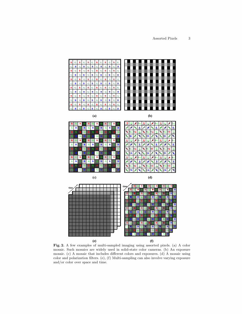
2. Figure 2(a) shows the popular Bayer mosaic [Bay76] of red, green and bluespectral filters placed adjacent to pixels on a detector. Since multiple color mea-surements cannot be captured simultaneously at a pixel, the pixels are assignedto specific colors to trade-off spatial resolution for spectral resolution. Over thelast three decades various color mosaics have been suggested, each one resultingin a different trade-off (see [Dil77], [Dil78], [MOS83], [Par85], [KM85]).

Historically, multi-sampled imaging has only been used in the form of colormosaics. Only recently has the approach been used to explore other imagingdimensions. Figure 2(b) shows the mosaic of neutral density filters with differenttransmittances used in [NM00] to enhance an image detector’s dynamic range.In this case, spatial resolution is traded-off for brightness resolution (dynamicrange). In [SN01], spatially varying transmittance and spectral filters were usedwith regular wide FOV mosaicing to yield high dynamic range and multi-spectralmosaics. Figure 2(c) shows how space, dynamic range and color can be sampledsimultaneously by using a mosaic of filters with different spectral responses andtransmittances. This type of multi-sampling is novel and, as we shall show,results in high dynamic range color images. Another example of assorted pixelswas proposed in [BE00], where a mosaic of polarization filters with differentorientations is used to estimate the polarization parameters of light reflected byscene points. This idea can be used in conjunction with a spectral mosaic, asshown in Figure 2(d), to achieve simultaneous capture of polarization and color.

Multi-sampled imaging can be exploited in many other ways. Figures 2(e)shows how temporal sampling can be used with exposure sampling. This ex-ample is related to the idea of sequential exposure change proposed in [MP95],[DM97] and [MN99] to enhance dynamic range. However, it is different in thatthe exposure is varied as a periodic function of time, enabling the generation ofhigh dynamic range, high framerate video. The closest implementation appearsto be the one described in [GHZ92] where the electronic gain of the camera isvaried periodically to achieve the same effect. A more sophisticated implementa-tion may sample space, time, exposure and spectrum, simultaneously, as shownin Figure 2(f).

The above examples illustrate that multi-sampling provides a general frame-work for designing imaging systems that extract information that is most per-

Assorted Pixels 3

R G R G R G R G R G R G






G B G B G B G B G B G B






R R R

R R R

R R R

B B B

B B B

B B B

G G G

G G G

G G G

G G G

G G G

G G G

R R R

R R R

R R R

B B B

B B B

B B B

G G G

G G G

G G G

G G G

G G G

G G G

R R R

R R R

R R R

B B B

B B B

B B B

G G G

G G G

G G G

G G G

G G G

G G G

R R R

R R R

R R R

B B B

B B B

B B B

G G G

G G G

G G G

G G G

G G G

G G G


















G R G R G R G R G R G








R G R G R R G R G

R R G R R G R R G

G R G R G R G

R R G R R G R G R G

R G R R G R R G R G





G G B G B G B G B G B










G B G B G G B G B G B




B

timetime

(a) (b)

(c) (d)

(e) (f)Fig. 2. A few examples of multi-sampled imaging using assorted pixels. (a) A colormosaic. Such mosaics are widely used in solid-state color cameras. (b) An exposuremosaic. (c) A mosaic that includes different colors and exposures. (d) A mosaic usingcolor and polarization filters. (e), (f) Multi-sampling can also involve varying exposureand/or color over space and time.


tinent to the application. Though our focus is on the visible light spectrum,multi-sampling is, in principle, applicable to any form of electromagnetic radia-tion. Therefore, the pixel assortments and reconstruction methods we describe inthis paper are also relevant to other imaging modalities such as X-ray, magneticresonance (MR) and infra-red (IR). Furthermore, the examples we discuss aretwo-dimensional but the methods we propose are directly applicable to higher-dimensional imaging problems such as ones found in tomography and microscopy.

2 Learned Structural Models for ReconstructionHow do we reconstruct the desired image from a captured multi-sampled one?Nyquist’s theory [Bra65] tells us that for a continuous signal to be perfectly re-constructed from its discrete samples, the sampling frequency must be at leasttwice the largest frequency in the signal. In the case of an image of a scene,the optical image is sampled at a frequency determined by the size of the de-tector and the number of pixels on it. In general, there is no guarantee thatthis sampling frequency satisfies Nyquist’s criterion. Therefore, when a tradi-tional interpolation technique is used to enhance spatial resolution, it is boundto introduce errors in the form of blurring and/or aliasing. In the case of multi-sampled images (see Figure 2), the assignment of pixels to multiple dimensionscauses further undersampling of scene radiance along at least some dimensions.As a result, conventional interpolation methods are even less effective.

Our objective is to overcome the limits imposed by Nyquist’s theory by usingprior models that capture redundancies inherent in images. The physical struc-tures of real-world objects, their reflectances and illuminations impose strongconstraints on the light fields of scenes. This causes different imaging dimen-sions to be highly correlated with each other. Therefore, a local mapping func-tion can be learned from a set of multi-sampled images and their correspondingcorrect (high quality) images. As we shall see, it is often beneficial to use multi-ple mapping functions. Then, given a novel multi-sampled image, these mappingfunctions can be used to reconstruct an image that has enhanced resolution ineach of the dimensions of interest. We refer to these learned mapping functionsas local structural models.

The general idea of learning interpolation functions is not new. In [FP99], aprobabilistic Markov network is trained to learn the relationship between sharpand blurred images, and then used to increase spatial resolution of an image.In [BK00], a linear system of equations is solved to estimate a high resolutionimage from a sequence of low resolution images wherein the object of interestis in motion. Note that both these algorithms are developed to improve spatialresolution, while our interest is in resolution enhancement along multiple imagingdimensions.

Learning based algorithms have also been applied to the problem of interpo-lating images captured using color mosaics. The most relevant among these isthe work of Wober and Soini [WS95] that estimates an interpolation kernel fromtraining data (high quality color images of test patterns and their correspond-ing color mosaic images). The same problem was addressed in [Bra94] using aBayesian method.

Assorted Pixels 5

We are interested in a general method that can interpolate not just colormosaic images but any type of multi-sampled data. For this, we propose the useof a structural model where each reconstructed value is a polynomial functionof the image brightnesses measured within a local neighborhood. The size of theneighborhood and the degree of the polynomial vary with the type of multi-sampled data being processed. It turns out that the model of Wober and Soini[WS95] is a special instance of our model as it is a first-order polynomial appliedto the specific case of color mosaic images. As we shall see, our polynomialmodel produces excellent results for a variety of multi-sampled images. Since ituses polynomials, our method is very efficient and can be easily implementedin hardware. In short, it is simple enough to be incorporated into any imagingdevice (digital still or video camera, for instance).

3 Training Using High Quality Images

Since we wish to learn our model parameters, we need a set of high qualitytraining images. These could be real images of scenes, synthetic images generatedby rendering, or some combination of the two. Real images can be acquired usingprofessional grade cameras whose performance we wish to emulate using lowerquality multi-sampling systems. Since we want our model to be general, the setof training images must adequately represent a wide range of scene features.For instance, images of urban settings, landscapes and indoor spaces may beincluded. Rotated and magnified versions of the images can be used to capturethe effects of scale and orientation. In addition, the images may span the gamutof illumination conditions encountered in practice, varying from indoor lightingto overcast and sunny conditions outdoor. Synthetic images are useful as onecan easily include in them specific features that are relevant to the application.

Fig. 3. Some of the 50 high quality images (2000 x 2000 pixels, 12 bits per colorchannel) used to train the local structural models described in Sections 4, 5 and 6.

Some of the 50 high quality images we have used in our experiments areshown in Figure 3. Each of these is a 2000 x 2000 color (red, green, blue) imagewith 12 bits of information in each color channel. These images were capturedusing a film camera and scanned using a 12-bit slide scanner. Though the total


number of training images is small they include a sufficiently large number oflocal (say, 7 × 7 pixels) appearances for training our structural models.

Given such high quality images, it is easy to generate a corresponding setof low-quality multi-sampled images. For instance, given a 2000 × 2000 RGBimage with 12-bits per pixel, per color channel, simple downsampling in space,color, and brightness results in a 1000 × 1000, 8 bits per pixel multi-sampledimage with the sampling pattern shown in Figure 2(c). We refer to this processof generating multi-sampled images from high quality images as downgrading.

With the high quality images and their corresponding (downgraded) multi-sampled images in place, we can learn the parameters of our structural model. Astructural model is a function f that relates measured data M(x, y) in a multi-sampled image to a desired value H(i, j) in the high quality training image:

H(i, j) = f(M(1, 1), ....,M(x, y), ....M(X, Y )) (1)

where, X and Y define some neighborhood of measured data around, or closeto, the high quality value H(i, j). Since our structural model is a polynomial, itis linear in its coefficients. Therefore, the coefficients can be efficiently computedfrom training data using linear regression.

Note that a single structural model may be inadequate. If we set aside themeasured data and focus on the type of multi-sampling used (see Figure 2), wesee that pixels can have different types of neighborhood sampling patterns. Ifwe want our models to be compact (small number of coefficients) and effectivewe cannot expect them to capture variations in scenes as well as changes in thesampling pattern. Hence, we use a single structural model for each type of localsampling pattern. Since our imaging dimensions are sampled in a uniform man-ner, in all cases we have a small number of local sampling patterns. Therefore,only a small number of structural models are needed. During reconstruction,given a pixel of interest, the appropriate structural model is invoked based onthe pixel’s known neighborhood sampling pattern.

4 Spatially Varying Color (SVC)

Most color cameras have a single image detector with a mosaic of red, green andblue spectral filters on it. The resulting image is hence a widely used type ofmulti-sampled image. We refer to it as a spatially varying color (SVC) image.When one uses an NTSC color camera, the output of the camera is nothing butan interpolated SVC image. Color cameras are notorious for producing inade-quate spatial resolution and this is exactly the problem we seek to overcomeusing structural models. Since this is our first example, we will use it to describesome of the general aspects of our approach.

4.1 Bayer Color Mosaic

Several types of color mosaics have been implemented in the past [Bay76], [Dil77],[Dil78], [MOS83], [Par85], [KM85]. However, the most popular of these is theBayer pattern [Bay76] shown in Figure 4. Since the human eye is more sensitiveto the green channel, the Bayer pattern uses more green filters than it does red

Assorted Pixels 7

and blue ones. Specifically, the spatial resolutions of green, red and blue are50%, 25% and 25%, respectively. Note that the entire mosaic is obtained byrepeating the 2 × 2 pattern shown on the right in Figure 4. Therefore, given aneighborhood size, all neighborhoods in a Bayer mosaic must have one of fourpossible sampling patterns. If the neighborhood is of size 3 × 3, the resultingpatterns are p1,p2, p3 and p4 shown in Figure 4.

R R R

R R R

R R R

B B B

B B B

B B B

G G G

G G G

G G G

G G G

G G G

G G G

p2

p4

p1

p3

R

B

G

G

2 x 2 Pattern

Fig. 4. Spatially varying color (SVC) pattern on a Bayer mosaic. Given a neighborhoodsize, all possible sampling patterns in the mosaic must be one of four types. In the caseof a 3 × 3 neighborhood, these patterns are p1, p2, p3 and p4.

4.2 SVC Structural ModelFrom the measured SVC image, we wish to compute three color values (red,green and blue) at each pixel, even though each pixel in the SVC image providesa single color measurement. Let the measured SVC image be denoted by Mand the desired high quality color image by H. A structural model relates eachcolor value in H to the measured data within a small neighborhood in M. Thisneighborhood includes measurements of different colors and hence the modelimplicitly accounts for correlations between different color channels.

As shown in Figure 5, let Mp be the measured data in a neighborhood withsampling pattern p, and Hp(i+0.5, j +0.5, λ) be the high quality color value atthe center of the neighborhood. (The center is off-grid because the neighborhoodis an even number of pixels in width and height.) Then, a polynomial structuralmodel can be written as:

Hp(i + 0.5, j + 0.5, λ) =∑

(x,y)∈Sp(i,j)

∑(k �=x,l �=y)∈Sp(i,j)

Np∑n=0

Np−n∑q=0

Cp(a, b, c, d, λ, n)Mpn(x, y) Mp

q(k, l) . (2)

Sp(i, j) is the neighborhood of pixel (i, j), Np is the order of the polynomialand Cp are the polynomial coefficients for the pattern p. The coefficient indices(a, b, c, d) are equal to (x − i, y − j, k − i, l − j).

The product Mp(x, y)Mp(k, l) explicitly represents the correlation betweendifferent pixels in the neighborhood. For efficiency, we have not used these cross-terms in our implementations. We found that very good results are obtained


R G

B

R

R R

B

B B

G

G G

G G

G G

B

RG

Mapping Function C

M ( x, y )p

H ( i+0.5, j+0.5, λ )p

( i+0.5, j+0.5 )

S ( i, j )pNeighborhoodReconstructed Values

Fig. 5. The measured data Mp in the neighborhood Sp(i, j) around pixel (i, j) arerelated to the high quality color values Hp(i + 0.5, j + 0.5, λ) via a polynomial withcoefficients Cp.

AH (λ)p p

p

pM

C (λ)

( with powers upto N )p

Fig. 6. The mapping function in (3) can be expressed as a linear system using matricesand vectors. For a given pattern p and color λ, Ap is the measurement matrix, Cp(λ)is the coefficient vector and Hp(λ) is the reconstruction vector.

even when each desired value is expressed as just a sum of polynomial functionsof the individual pixel measurements:

Hp(i + 0.5, j + 0.5, λ) =∑

(x,y)∈Sp(i,j)

Np∑n=0

Cp(a, b, λ, n)Mpn(x, y). (3)

The mapping function (3), for each color λ and each local pattern type p,can be conveniently rewritten using matrices and vectors, as shown in Figure 6:

Hp(λ) = Ap Cp(λ) . (4)

For a given pattern type p and color λ, Ap is the measurement matrix. Therows of Ap correspond to the different neighborhoods in the image that have thepattern p. Each row includes all the relevant powers (up to Np) of the measureddata Mp within the neighborhood. The vector Cp(λ) includes the coefficientsof the polynomial mapping function and the vector Hp(λ) includes the desiredhigh quality values at the off-grid neighborhood centers. The estimation of themodel parameters Cp can then be posed as a least squares problem:

Cp(λ) = (ATp Ap)−1AT

p Hp(λ) , (5)

When the signal-to-noise characteristics of the image detector are known, (5) canbe rewritten using weighted least squares to achieve greater accuracy [Aut01].

Assorted Pixels 9

4.3 Total Number of Coefficients

The number of coefficients in the model (3) can be calculated as follows. Letthe neighborhood size be u× v, and the polynomial order corresponding to eachpattern p be Np. Let the number of distinct local patterns in the SVC image beP and the number of color channels be Λ. Then, the total number of coefficientsneeded for structural interpolation is:

|C| =

(P + u ∗ v ∗

P∑p=1

Np

)∗ Λ . (6)

For the Bayer mosaic, P = 4 and Λ = 3 (R,G,B). If we use Np = 2 andu = v = 6, the total number of coefficients is 876. Since these coefficients arelearned from real data, they yield greater precision during interpolation thanstandard interpolation kernels. In addition, they are very efficient to apply. Sincethere are P = 4 distinct patterns, only 219 (a quarter) of the coefficients are usedfor computing the three color values at a pixel. Note that the polynomial modelis linear in the coefficients. Hence, structural interpolation can be implementedin real-time using a set of linear filters that act on the captured image and itspowers (up to Np).

4.4 Experiments

A total of 30 high quality training images (see Figure 3) were used to computethe structural model for SVC image interpolation. Each image is downgradedto obtain a corresponding Bayer-type SVC image. For each of the four samplingpatterns in the Bayer mosaic, and for each of the three colors, the appropriateimage neighborhoods were used to compute the measurement matrix Ap and thereconstruction vector Hp(λ). While computing these, one additional step wastaken; each measurement is normalized by the energy within its neighborhoodto make the structural model insensitive to changes in illumination intensityand camera gain. The resulting Ap and Hp(λ) are used to find the coefficientvector Cp(λ) using linear regression (see (5)). In our implementation, we usedthe parameter values P = 4 (Bayer), Np = 2, u = v = 6 and Λ = 3 (R,G, B),to get a total of 876 coefficients.

The above structural model was used to interpolate 20 test SVC images thatare different from the ones used for training. In Figure 7(a), a high quality (8-bits per color channel) image is shown. Figure 7(b) shows the corresponding(downgraded) SVC image. This is really a single channel 8-bit image and itspixels are shown in color only to illustrate the Bayer pattern. Figure 7(c) showsa color image computed from the SVC image using bi-cubic interpolation. As isusually done, the three channels are interpolated separately using their respectivedata in the SVC image. The magnified image region clearly shows that bi-cubicinterpolation results in a loss of high frequencies; the edges of the tree branchesand the squirrels are severely blurred. Figure 7(d) shows the result of applyingstructural interpolation. Note that the result is of high quality with minimal lossof details.


(a)

(b)

(c)

(d)

0 2 4 6 8 10 12 14 16 18 20

0

2

4

6

8

10

12

x 104

Structural Model

Bi-Cubic Interpolation

Pixels

RMSError

(e)

Fig. 7. (a) Original (high quality) color image with 8-bits per color channel. (b) SVCimage obtained by downgrading the original image. The pixels in this image are shownin color only to illustrate the Bayer mosaic. Color image computed from the SVCimage using (c) bi-cubic interpolation and (d) structural interpolation. (e) Histogramsof luminance error (averaged over 20 test images). The RMS error is 6.12 gray levelsfor bi-cubic interpolation and 3.27 gray levels for structural interpolation.

Assorted Pixels 11

We have quantitatively verified of our results. Figure 7(e) shows histograms ofthe luminance error for bi-cubic and structural interpolation. These histogramsare computed using all 20 test images (not just the one in Figure 7). Thedifference between the two histograms may appear to be small butis significant because a large fraction of the pixels in the 20 imagesbelong to “flat” image regions that are easy to interpolate for bothmethods. The RMS errors (computed over all 20 images) are 6.12 and 3.27 graylevels for bi-cubic and structural interpolation, respectively.

5 Spatially Varying Exposures (SVE)

In [NM00], it was shown that the dynamic range of a gray-scale image detectorcan be significantly enhanced by assigning different exposures (neutral densityfilters) to pixels, as shown in Figure 8. This is yet another example of a multi-sampled image and is referred to as a spatially varying exposure (SVE) image. In[NM00], standard bi-cubic interpolation was used to reconstruct a high dynamicrange gray-scale image from the captured SVE image; first, saturated and darkpixels are eliminated, then all remaining measurements are normalized by theirexposure values, and finally bi-cubic interpolation is used to find the brightnessvalues at the saturated and dark pixels. As expected, the resulting image hasenhanced dynamic range but lower spatial resolution. In this section, we applystructural interpolation to SVE images and show how it outperforms bi-cubicinterpolation.

e

e

ee

1

4

3

2

p4

p3

p1

p2

Fig. 8. The dynamic range of an image detector can be improved by assigning differentexposures to pixels. In this special case of 4 exposures, any 6 × 6 neighborhood in theimage must belong to one of four possible sampling patterns shown as p1 . . .p4.

5.1 SVE Structural Model

As in the SVC case, let the measured SVE data be M and the correspondinghigh dynamic range data be H. If the SVE detector uses only four discreteexposures (see Figure 8), it is easy to see that a neighborhood of any given sizecan have only one of four different sampling patterns (P = 4). Therefore, foreach sampling pattern p, a polynomial structural model is used that relates thecaptured data Mp within the neighborhood to the high dynamic range valueHp at the center of the neighborhood:

Hp(i + 0.5, j + 0.5) =∑

(x,y)∈Sp(i,j)

Np∑n=0

Cp(a, b, n) Mpn(x, y) , (7)


where, as before, (a, b) = (x − i, y − j), Sp(i, j) is the neighborhood of pixel(i, j), Np is the order of the polynomial mapping, and Cp are the polynomialcoefficients for the pattern p. Note that there is only one channel in this case(gray-scale) and hence the parameter λ is omitted. The above model is rewrittenin terms of a measurement matrix Ap and a reconstruction vector Hp, andthe coefficients Cp are found using (5). The number of coefficients in the SVEstructural model is determined as:

|C| = P + u ∗ v ∗P∑

p=1

Np . (8)

In our implementation, we have used P = 4, Np = 2 and u = v = 6, whichgiven a total of 292 coefficients. Since P = 4, only 73 coefficients are needed forreconstructing each pixel in the image.

5.2 Experiments

The SVE structural model was trained using 12-bit gray-scale versions of 6 ofthe images shown in Figure 3 and their corresponding 8-bit SVE images. EachSVE image was obtained by applying the exposure pattern shown in Figure 8(with e4 = 4e3 = 16e2 = 64e1) to the original image, followed by a downgradefrom 12 bits to 8 bits. The structural model was tested using 6 test images, oneof which is shown in Figure 9. Figure 9(a) shows the original 12-bit image, Figure9(b) shows the downgraded 8-bit SVE image, Figure 9(c) shows a 12-bit imageobtained by bi-cubic interpolation of the SVE image, and Figure 9(d) shows the12-bit image obtained by structural interpolation. The magnified images shownon the right are histogram equalized to bring out the details (in the clouds andwalls) that are lost during bi-cubic interpolation but extracted by structuralinterpolation. Figure 9(e) compares the error histograms (computed using all6 test images) for the two cases. The RMS errors were found to be 33.4 and25.5 gray levels (in a 12-bit range) for bi-cubic and structural interpolations,respectively. Note that even though a very small number (6) of images wereused for training, our method outperforms bi-cubic interpolation.

6 Spatially Varying Exposure and Color (SVEC)

Since we are able to extract high spatial and spectral resolution from SVC imagesand high spatial and brightness resolution from SVE images, it is natural toexplore how these two types of multi-sampling can be combined into one. Theresult is the simultaneous sampling of space, color and exposure (see Figure 10).We refer to an image obtained in this manner as a spatially varying exposureand color (SVEC) image. If the SVEC image has 8-bits at each pixel, we wouldlike to compute at each pixel three color values, each with 12 bits of precision.Since the same number of pixels on a detector are now being used to samplethree different dimensions, it should be obvious that this is a truly challenginginterpolation problem. We will see that structural interpolation does remarkablywell at extracting the desired information.

Assorted Pixels 13

(a)

(b)

(c)

(d)

RMSError

Pixels

0 10 20 30 40 50 60 70 80 90 100

0

2

4

6

8

10

12

x 104

Structural Model


(e)

Fig. 9. (a) Original 12-bit gray scale image. (b) 8-bit SVE image. (c) 12-bit (highdynamic range) image computed using bi-cubic interpolation. (d) 12-bit (high dynamicrange) image computed using structural models. (d) Error histograms for the two case(averaged over 6 test images). The RMS error for the 6 images are 33.4 and 25.5 graylevels (on a 12-bit scale) for bi-cubic and structural interpolation, respectively. Themagnified image regions on the right are histogram equalized.


R G R G

R G R G

R G R G

R G R G

R G R G

R G R G

G B G B

G B G B

G B G B

G B G B

G B G B

G B G B

R G R G

R G R G

G B G B

G B G B

















p9

p10

p5

p1 p6 p2 p7 p3 p8

p12

p16

p11p4

p13

p14

p15

Fig. 10. A combined mosaic of 3 spectral and 4 neutral density filters used to simulta-neously sample space, color and exposures using a single image detector. The captured8-bit SVEC image can be used to compute a 12-bit (per channel) color image bystructural interpolation. For this mosaic, for any neighborhood size, there are only 16distinct sampling patterns. For a 4× 4 neighborhood size, the patterns are p1 . . .p16.

Color and exposure filters can be used to construct an SVEC sensor in manyways. All possible mosaics that can be constructed from Λ colors and E exposuresare derived in [Aut01]. Here, we will focus on the mosaic shown in Figure 10,where 3 colors and 4 exposures are used. For any given neighborhood size, it isshown in [Aut01] that only 16 different sampling patterns exist (see Figure 10).

6.1 SVEC Structural Model

The polynomial structural model used in the SVEC case is the same as the oneused for SVC, and is given by (3). The only caveat is that in the SVEC case weneed to ensure that the neighborhood size used is large enough to adequatelysample all the colors and exposures. That is, the neighborhood size is chosensuch that it includes all colors and all exposures of each color.

The total number of polynomial coefficients needed is computed the sameway as in the SVC case and is given by (6). In our experiments, we have usedthe mosaic shown in Figure 10. Therefore, P = 16, Λ = 3 (R, G, and B), Np = 2for each of the 16 patterns, and u = v = 6, to give a total of 3504 coefficients.Once again, at each pixel, for each color, only 3504/48 = 73 coefficients are used.Therefore, even for this complex type of multi-sampling, our structural modelscan be applied to images in real-time using a set of linear filters.

6.2 Experiments

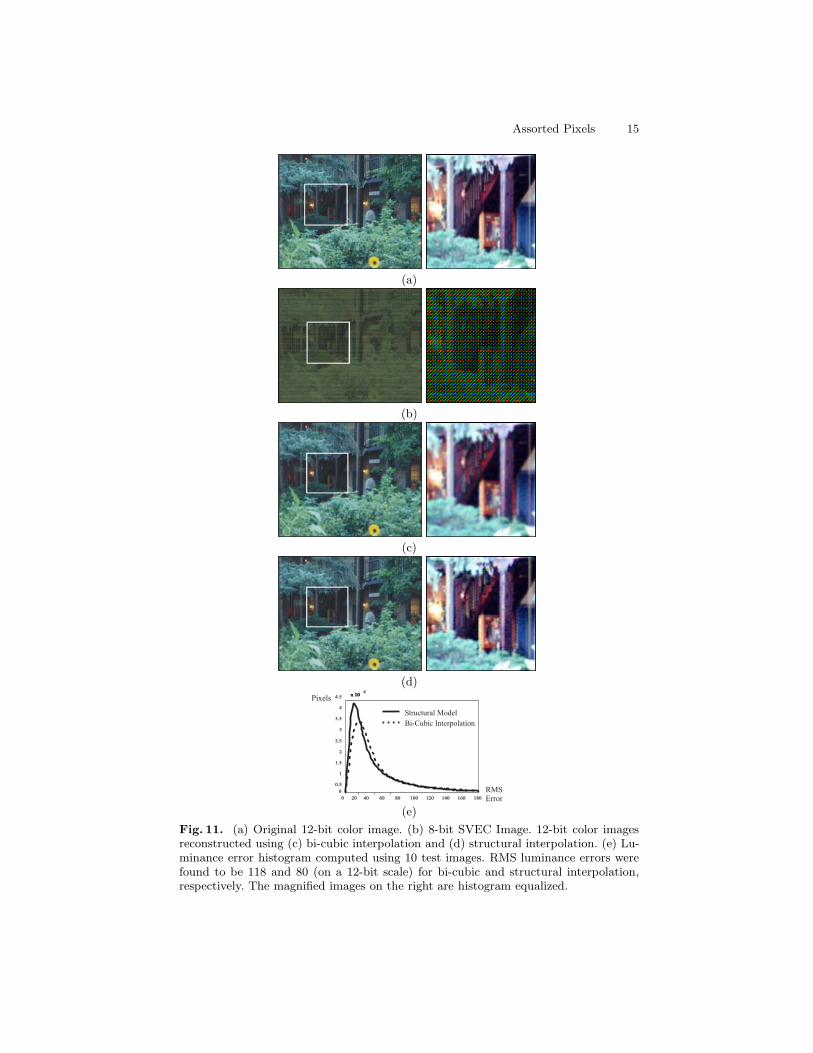
The SVEC structural model was trained using 6 of the images in Figure 3. Inthis case, the 12-bit color images in the training set were downgraded to 8-bitSVEC images. The original and SVEC images were used to compute the 3504coefficients of the model. The model was then used to map 10 different testSVEC images to 12-bit color images. One of these results is shown in Figure11. The original 12-bit image shown in Figure 11(a) was downgraded to obtainthe 8-bit SVEC image shown in Figure 11(b). This image has a single channel

Assorted Pixels 15

(a)

(b)

(c)

(d)

RMSError

Pixels

0 20 40 60 80 100 120 140 160 180

0

0.5

1

1.5

2

2.5

3

3.5

4

4.5 x 10x 104

Structural Model


(e)

Fig. 11. (a) Original 12-bit color image. (b) 8-bit SVEC Image. 12-bit color imagesreconstructed using (c) bi-cubic interpolation and (d) structural interpolation. (e) Lu-minance error histogram computed using 10 test images. RMS luminance errors werefound to be 118 and 80 (on a 12-bit scale) for bi-cubic and structural interpolation,respectively. The magnified images on the right are histogram equalized.


and is shown here in color only to illustrate the effect of simultaneous color andexposure sampling. Figures 11(c) and (d) show the results of applying bi-cubicand structural interpolation, respectively. It is evident from the magnified imageson the right that structural interpolation yields greater spectral and spatialresolution. The two interpolation techniques are compared in Figure 11(e) whichshows error histograms computed using all 10 test images. The RMS luminanceerrors were found to be 118 gray-levels and 80 gray-levels (on a 12 bit scale) forbi-cubic and structural interpolations, respectively.

Acknowledgements: This research was supported in parts by a ONR/ARPAMURI Grant (N00014-95-1-0601) and an NSF ITR Award (IIS-00-85864).

References

[Aut01] Authors. Resolution Enhancement Along Multiple Imaging Dimensions UsingStructural Models. Technical Report, Authors’ Institution, 2001.

[Bay76] B. E. Bayer. Color imaging array. U.S. Patent 3,971,065, July 1976.[BE00] M. Ben-Ezra. Segmentation with Invisible Keying Signal. In CVPR, 2000.[BK00] S. Baker and T. Kanade. Limits on Super-Resolution and How to Break

Them. In Proc. of CVPR, pages II:372–379, 2000.[Bra65] R. N. Bracewell. The Fourier Transform and Its Applications. McGraw Hill,

1965.[Bra94] D. Brainard. Bayesian method for reconstructing color images from trichro-

matic samples. In Proc. of IS&T 47th Annual Meeting, pages 375–380,Rochester, New York, 1994.

[Dil77] P. L. P. Dillon. Color imaging array. U.S. Patent 4,047203, September 1977.[Dil78] P. L. P Dillon. Fabrication and performance of color filter arrays for solid-

state imagers. In IEEE Trans. on Electron Devices, volume ED-25, pages97–101, 1978.

[DM97] P. Debevec and J. Malik. Recovering High Dynamic Range Radiance Mapsfrom Photographs. Proc. of ACM SIGGRAPH 1997, pages 369–378, 1997.

[FP99] W. Freeman and E. Pasztor. Learning Low-Level Vision. In Proc. of ICCV,pages 1182–1189, 1999.

[GHZ92] R. Ginosar, O. Hilsenrath, and Y. Zeevi. Wide dynamic range camera. U.S.Patent 5,144,442, September 1992.

[KM85] K. Knop and R. Morf. A new class of mosaic color encoding patterns forsingle-chip cameras. In IEEE Trans. on Electron Devices, volume ED-32,1985.

[MN99] T. Mitsunaga and S. K. Nayar. Radiometric Self Calibration. In Proc. ofCVPR, pages I:374–380, 1999.

[MOS83] D. Manabe, T. Ohta, and Y. Shimidzu. Color filter array for IC image sensor.In Proc. of IEEE Custom Integrated Circuits Conference, pages 451–455, 1983.

[MP95] S. Mann and R. Picard. Being ‘Undigital’ with Digital Cameras: ExtendingDynamic Range by Combining Differently Exposed Pictures. Proc. of IST’s48th Annual Conf., pages 442–448, May 1995.

[NM00] S. K. Nayar and T. Mitsunaga. High Dynamic Range Imaging: SpatiallyVarying Pixel Exposures. In Proc. of CVPR, pages I:472–479, 2000.

[Par85] K. A. Parulski. Color filters and processing alternatives for one-chip cameras.In IEEE Trans. on Electron Devices, volume ED-32, 1985.

[SN01] Y. Y. Schechner and S. K. Nayar. Generalized mosaicing. In ICCV, 2001.[WS95] M. A. Wober and R. Soini. Method and apparatus for recovering image data

through the use of a color test pattern. U.S. Patent 5,475,769, Dec. 1995.

assorted pixels: multi-sampled imaging with structural models

Documents