Assumptions

Gary W. Oehlert

School of StatisticsUniversity of Minnesota

February 7, 2016

Background

Our inference tools make assumptions. We assume that

yij = µ+ αi + εij

where the εijs are independent with distribution N(0, σ2).1

If the model is correct, our inference is good and matches with randomizationinference.

Unfortunately, wishing doesn’t make it so.

1Equivalently, we can say that yij follows N(µi , σ2).

If the assumptions are not true, our inferences might not be valid, for example,

A confidence interval might not cover with the stated error rate.

A test with nominal type I error of E could actually have a larger or smaller type Ierror rate.

This is obviously bad news and can be the source of controversy and disagreementover how the analysis was done and the validity of the results.

(But if you did a randomization, your randomization inference is still valid.)

Some procedures work reasonably well (e.g., actual interval coverage rate is near tonominal, or actual p-value is close to nominal p-value) even when some assumptionsare violated.

This is called robustness of validity.

Generally these procedures work better when violations are mild and work less well asviolations become more extreme.

A procedure that has robustness of validity can be inefficient, so we might not want touse it even if it is robust.

The basic assumptions are

Independence (most important)

Constant variance

Normality (least important)

Many ways that data can fail to be independent; we will learn to check for one.

In this course we will not generally try to fix or accommodate dependence. We leavethat for other courses (e.g., time series, multivariate analysis, etc.).

Residuals

To make matters interesting, our assumptions are about the εij , but we never get tosee them. They are unobservable, so we must guide our analysis using something else.

What we do have are residuals.

The basic raw residual isrij = yij − fitted value

In our simple models to date that is

rij = yij − (µ̂+ α̂i ) = yij − y i•

The raw residual is useful for many purposes, and is often good enough in balanceddesigned experiments. However, we can do better.

The standardized residual (sometimes called internally Studentized) adjusts rij for itsestimated standard deviation:

sij =rij√

MSE (1− Hij)

The Hij value is called the leverage; it is a diagonal element of the “Hat” matrix,which is why we call it H. Use hatvalues() in R.

Roughly speaking, the sij should look like standard normals, particularly in largesamples.

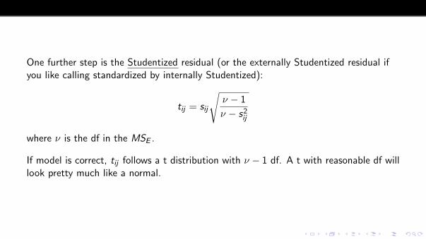
One further step is the Studentized residual (or the externally Studentized residual ifyou like calling standardized by internally Studentized):

tij = sij

√ν − 1

ν − s2ij

where ν is the df in the MSE .

If model is correct, tij follows a t distribution with ν − 1 df. A t with reasonable df willlook pretty much like a normal.

Studentized residuals are especially good in looking for outliers.

Think of adding a dummy variable to a model that is 1 for point i,j and 0 otherwise.The t-test for the coefficient of that dummy variable is the Studentized residual in theoriginal model.

Studentized residuals say how well the data value fits the model estimated from therest of the data.

Assessing assumptions

I don’t like to test for normality or constant variance etc.:

With small sample sizes, you’ll never be able to reject the null that there are noproblems.

With large sample sizes, you’ll constantly detect little problems that have nopractical effect.

It’s really all shades of gray (at least 50), and we would like to know where we are onthe scale from mild issues to severe issues.

So assess assumptions qualitatively; don’t just rely on a test.

Residual plots

Our principal tools for assessing assumptions are various plots of residuals:

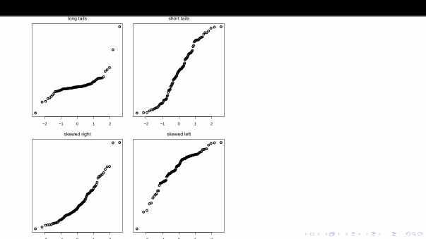
Normal probability plot

Residuals versus predicted plot

Residuals in time order

The first two are the basic plots for assessing normality and constant variance; the lastone is just one of many potential plots for assessing independence.

The NPP plots the residual against its corresponding normal score. The smallestresidual plots against the smallest normal score for a sample of N; the second smallestresidual against the second smallest normal score, and so on.

Normal scores depend on N. Think about an independent sample of N standardnormals. They all have mean 0, but if you just consider the smallest one, it has anegative expectation. That expectation is its normal score.

The rankit approximates the normal score:

rankiti ,N = Φ−1

(i − 3/8

n + 1/4

)where Φ−1 gives normal percent points.

It’s probably best to use the Studentized residuals, but the others also work fine inmost situations.

Normally distributed data (and, we hope, residuals from iid normally distributed errors)should have a roughly linear shape, although even normal data can look crooked insmall samples.

You can tell the shape of the data from the shape of the plot, but you need to practice(and you will).

●

●●●

●

●

●

●

●

●●

●

●

●

●

●

●

●

●

●

●●

●

●

●

●

● ●

●

●

● ●

●

●●

●●● ●

●●

● ●●

●

●●●

●●

●

●

●

●

●

●● ●

●

●

●●●

●

●

●

●●

●●●

●

●

●●●

●●

●

●

●

● ●

●

●

●●●

●

●

●●

● ●● ● ●

●

●●

−2 −1 0 1 2

long tails

●

●

●

●

●

●

●

●

●

●

●

●

●

●

●

●

●

●

●

●

●

●●

●

●

●

●

●

●

●●

●

●

●

●

●

●

●

●●

●

●

●

●

●

●

●

●

●

●

●

●

●

●

●

●

●

●

●

●

●

●

●

●

●

●

●

●

●

●

●

●

●

●

●

●

●●

●

●

●

●

●

●

●

●

●

●

●

●

●

●

●

●

●●

●

●●

●

−2 −1 0 1 2

short tails

●

●

●

●●

●

●

●

●

●

●

●

●

●

●

●

●

●

●

●

●

●

●

●

●●

●

●

●

●

●

●

●●●

●

●

●

●

●

●

●

●

●

●

●

●

●

●

●

●

●

●

●

●

●

●

●

●

●

●●●

●

●

●●

●

●

●

●

●

●●

●

●

●

●●

●

●

●

●

●

●

●

●●

●

●

●

●

●

●

●

●

●

●

●

●

−2 −1 0 1 2Theoretical Quantiles

skewed right

●

●

●

●●

●

●●

●

●

●

●

●

●

●

●●

●

●

●

●

●

●

●

●

●

●

●

●

●

●●

●

●

●

●

●●

●●

●

●

●

●

●

●

●

●

●

●

●

●●

●

●

●

●

●

●

●

●

●

●

●

●

●

●●

●

●

●

●

●●

●●

●

●

●

●

●

●

●●

●

●

●

●

●

●●

●

●

●

●

●

●

●

●

●

−2 −1 0 1 2Theoretical Quantiles

skewed left

●

●

●

●

●

●

●

●

●

●

●

●

●

●

●

●

●

●

●

●

−2 −1 0 1 2

iid Normal

●

●

●

●

●

●

●

●

●

●●

●

●

●

●

● ●

●

●

●

−2 −1 0 1 2

iid Normal

●

●

●

●

●

●

●

●

●

●

●

●●

●

●

●

●

●

●

●

−2 −1 0 1 2

iid Normal

●

●

●

●

●

●

●

●

●

●

●

●

●

●●

●

●

●

●

●

−2 −1 0 1 2

iid Normal

You can also test for outliers using the Studentized residuals (the t-residuals).

These are a one-at-a-time test. Look at the largest absolute t-residual and then do thetest by making a Bonferroni adjustment (i.e., multiply p-value by N, if it still lookssmall, then you have an outlier).

You can do this sequentially, but the test is only exact for the first one.

The diagnostic plot for non-constant variance is to plot each residual against itscorresponding predicted/fitted value.

We are hoping to see no pattern in the vertical dispersion.

The most common problem occurs when larger means go with larger variances. In thiscase we see a “right opening megaphone.”

We sometimes see the reverse, particularly when there is an upper bound on theresponse.

There are several variations on this, including box plots of residuals and plots of squareroot absolute residuals against fitted values.

If you have to/want to test for equality of variances, your best bet is Levene’s test.This makes a new response as the absolute value of the deviations of the original datafrom the predicted value, and then does an ANOVA test for the separate means modelon the absolute deviations.

There are several variations on this where you might take absolute deviations from themedian of each group, or the absolute deviations to some power, etc.

There are several classical tests of equality of variance including Barlett’s test andHartley’s test; avoid them like the plague! They are incredibly hyper-sensitive tonormality.

Back to the resin example in R.

There are many ways that data could fail to be independent, but we will only talkabout the simplest of these: temporal dependence.

In some data sets, but not all data sets, there is a time order of some kind.

One common failure of independence is when data close in time tend to have similarεijs and thus similar residuals. This is called positive temporal dependence or positiveserial correlation.

The reverse can also happen (near in time tend to be unusually far apart), but it ismuch more rare.

The simplest diagnostic is to plot the residuals in time order and look for patterns.

Do the residuals seem to be high and low together in patches? That is positive serialcorrelation.

Do the residuals seem to bounce up and down very roughly and alternately? Thatcould be negative serial correlation.

The stronger the pattern, the stronger the correlation and the greater the problem itwill cause with inference.

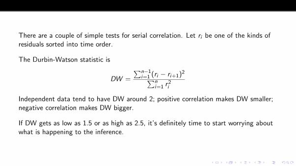
There are a couple of simple tests for serial correlation. Let ri be one of the kinds ofresiduals sorted into time order.

The Durbin-Watson statistic is

DW =

∑n−1i=1 (ri − ri+1)2∑n

i=1 r2i

Independent data tend to have DW around 2; positive correlation makes DW smaller;negative correlation makes DW bigger.

If DW gets as low as 1.5 or as high as 2.5, it’s definitely time to start worrying aboutwhat is happening to the inference.

There are also a whole variety of “runs” tests, variously defined. These look for thingslike runs of residuals that are positive (or negative), or runs of data that are increasing(or decreasing).

In any event, there are several runs tests, but they can also be used to assess temporalcorrelation.

Only assess temporal correlation if your data have a time order!

Accommodating problems

There are two basic approaches to dealing with things when assumptions are not met:

Alternate methods

Massaging the data

Developing alternate methods is basically a full-employment act for academicstatisticians. The problem is that there are so many things we want to do with ourstandard approaches, that developing alternatives is also difficult and very timeconsuming (and life would be really difficult for the non-academics).

I’ll mention a few broad areas, but only talk about a couple alternatives.

Robustness is a philosophy and class of techniques that deal with long-tailed, outlierprone data.

Generalized Linear Models (GLM) is a class of techniques for using models with linearpredictors but which have non-normal data including count data and various kinds ofnon-constant variance.

Time series is a class of statistical models for working with serial correlation (amongother things).

Spatial statistics includes, among other things, the ability to fit linear models when thedata are correlated in space.

Direct replacements are usually developed to solve specific narrow issues withoutbuilding a whole new class of statistical models.

Many of you are familiar with the version of the t-test that does not use a pooledestimate of variance. Instead, it uses

t =y i• − y j•√

s2ini

+s2jnj

where s2i and s2j are the sample variances in two groups. There is a formula forapproximate df, and then you compare with a t-distribution.

This is the direct replacement for ANOVA when g=2 and there is non-constantvariance.

In this case, the replacement is so easy and works so well that there is little reason notto use it all the time.

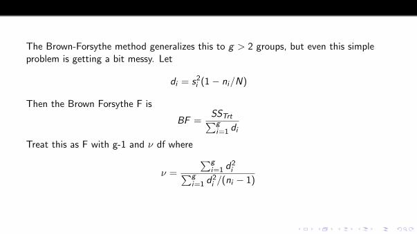
The Brown-Forsythe method generalizes this to g > 2 groups, but even this simpleproblem is getting a bit messy. Let

di = s2i (1− ni/N)

Then the Brown Forsythe F is

BF =SSTrt∑gi=1 di

Treat this as F with g-1 and ν df where

ν =

∑gi=1 d

2i∑g

i=1 d2i /(ni − 1)

Massaging the data

This sounds like iniquity, but it’s really not that bad.

The simplest form of this practice is removing outliers and reanalyzing the data.Ideally, we would like to get the same basic inference with and without the outliers.

If the inference changes substantially, this means that it is dependent on just a handfulof the data.

You can’t automatically reject a data value simply because it does not fit the modelyou assume.

Our go-to approach is usually to transform the data, that is, to re-express the data onanother scale. Thus we might use

pH instead of hydrogen ion concentration (log transformation);

diameter of a bacterial colony rather than area (square root transformation);

time to distance instead of rate of advance (reciprocal transformation).

In general, any monotone transformation will work, but we concentrate on powerfamily transformations.

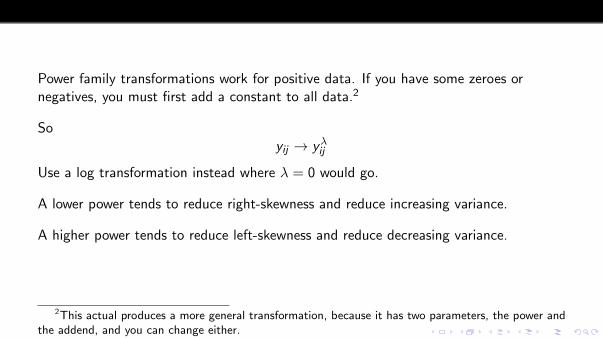
Power family transformations work for positive data. If you have some zeroes ornegatives, you must first add a constant to all data.2

Soyij → yλij

Use a log transformation instead where λ = 0 would go.

A lower power tends to reduce right-skewness and reduce increasing variance.

A higher power tends to reduce left-skewness and reduce decreasing variance.

2This actual produces a more general transformation, because it has two parameters, the power andthe addend, and you can change either.

Note: if the data only range over a factor of 2 or 3, then power transformations are oflimited utility. As the ratio of largest to smallest increases, power transformations canhave more effect.

Serendipity. More often than we have any right to expect, transformations that makevariance more constant also improve normality.

However, if I have to choose between the two, I generally go for more constantvariance at the cost of worse normality.

The Box-Cox procedure helps us

Pick a reasonable range of transformation powers

Decide whether we need a transformation

I try not to be a slave to the Box-Cox test, and I also try to pick a transformationpower that both fixes the problems and is also interpretable. But it is still a very usefulguide.

In R, Box-Cox gives us a likelihood profile for λ as well as a 95% confidence interval.

−2 −1 0 1 2

−19

0−

180

−17

0−

160

−15

0−

140

−13

0

λ

log−

Like

lihoo

d

95%

R examples.

Inference

If the null is that distributions in different treatments are the same on one scale, theywill also be the same on some other scale.

We might as well use the one where are assumptions are plausible.

We can test equality of means on any scale and get proper inference.

That’s the good news . . .

The bad news shows up when you want to make inference on means across scales.

Means do not transform cleanly across power transformations.

That is, you cannot exponentiate the mean of the log data to get the mean of thenatural scale data.

A transformed CI for the mean of normal data is a CI for the median on thetransformed scale, not for the mean.

Land’s method helps in the specific case of logs and anti-logs, but in general you eithermake due with medians or work on the original scale and take you lumps on the qualityof inference.

Consequences

So how bad is this, really?

Skewness measures how asymmetric a distribution is.Kurtosis measures how long-tailed (outlier prone) a distribution is.The normal has both 0 skewness and 0 kurtosis.

Absent outliers, F-test is only slightly affected by non-normality.

F-test has reasonable robustness of validity, but it is not resistant; individual outlierscan change test results.

Often check to see if inference is consistent with and without outliers.

For balanced data (all sample sizes equal),

Skewness has little effect

Long tails (positive kurtosis) leads to conservative tests. These tests have nominalp-values larger than they really should be, so fewer rejections than we should have.

Short tails (negative kurtosis) leads to liberal tests. These tests have nominalp-values smaller than they really should be, so more rejections than we shouldhave.

Table 6.5 gives some numerical results.

Inconsistent results for unbalanced data.

Smaller effects in larger data sets.

Skewness and kurtosis for selected distributions

Distribution γ1 γ2

Normal 0 0

Uniform 0 -1.2

Normal truncated at±1 0 -1.06±2 0 -0.63

Student’s t (df)5 0 66 0 38 0 1.520 0 .38

Chi-square (df)1 2.83 122 2 64 1.41 38 1 1.5

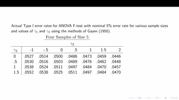
Actual Type I error rates for ANOVA F-test with nominal 5% error rate for various sample sizes

and values of γ1 and γ2 using the methods of Gayen (1950).

Four Samples of Size 5

γ2

γ1 -1 -.5 0 .5 1 1.5 2

0 .0527 .0514 .0500 .0486 .0473 .0459 .0446.5 .0530 .0516 .0503 .0489 .0476 .0462 .04481 .0538 .0524 .0511 .0497 .0484 .0470 .04571.5 .0552 .0538 .0525 .0511 .0497 .0484 .0470

γ1 = 0 and γ2 = 1.5

4 groups of k k groups of 5 (k1, k1, k2, k2)

k Error k Error k1, k2 Error

2 .0427 4 .0459 10,10 .048010 .0480 8 .0474 8,12 .048320 .0490 16 .0485 5,15 .050040 .0495 32 .0492 2,18 .0588

Skewness can really mess up one-sided confidence intervals. I mean bad.

Two-sided intervals are less affected by skewness, but the coverage errors may pile upon one side.

Pairwise comparisons with balanced data are generally doing well (the differencingtends to cancel the skewness).

Non-constant variance can have serious effects, although the effects are smaller forbalanced designs.

If big ni s go with big σ2i s, you get a conservative test that does not reject oftenenough. (The big variances are “over represented” in our standard MSE.)

If big ni s go with small σ2i s, you get a liberal test that rejects too often. (The smallvariances are “over represented” in our standard MSE.)

Table 6.6 shows some examples of how bad things can get with non-constant variance.

For the settings in that table, nominal 5% tests are actually somewhere between 3%and 20%.

More data does not fix the problem.

For pairwise comparisons, some will be liberal and others will be conservative.

g σ2i ni E

3 1, 1, 1 5, 5, 5 .051, 2, 3 5, 5, 5 .05791, 2, 5 5, 5, 5 .06851, 2, 10 5, 5, 5 .08641, 1, 10 5, 5, 5 .09541, 1, 10 50, 50, 50 .0748

3 1, 2, 5 2, 5, 8 .02021, 2, 5 8, 5, 2 .18331, 2, 10 2, 5, 8 .01781, 2, 10 8, 5, 2 .28311, 2, 10 20, 50, 80 .01161, 2, 10 80, 50, 20 .2384

5 1, 2, 2, 2, 5 5, 5, 5, 5, 5 .06821, 2, 2, 2, 5 2, 2, 5, 8, 8 .02921, 2, 2, 2, 5 8, 8, 5, 2, 2 .14531, 1, 1, 1, 5 5, 5, 5, 5, 5 .09081, 1, 1, 1, 5 2, 2, 5, 8, 8 .03471, 1, 1, 1, 5 8, 8, 5, 2, 2 .2029

Outcomes with dependent data depend extremely delicately on the exact nature of thedependence and the exact nature of the contrast or test.

For example, if data are sequential in time with neighboring εs correlated .4, then anominal 95% confidence interval could have coverage 86% or 99.9% depending onwhether the treatments were done in blocks or alternately.

More data does not help.

Randomization does help. If you had randomized the order of the treatments, then thecoverage would have been between 95.5% and 94.6%, which is certainly good enough.

Between what we see here and what we saw for non-normality and non-constantvariance, it looks like randomized, balanced designs are least susceptible to violationsof assumptions.

Error rates ×100 of nominal 95% confidence intervals for µ1 − µ2, when neighboringdata values have correlation ρ and data patterns are consecutive or alternate.

ρ–.3 –.2 –.1 0 .1 .2 .3 .4

Con. .19 1.1 2.8 5 7.4 9.8 12 14Alt. 12 9.8 7.4 5 2.8 1.1 .19 .001

All this should make you wonder about people who obsess over whether the p-value is.051 or .049.

Little, undetectable bits of non-normality, non-constant variance, or dependence caneasily swing the p-value much more than that.