astrophysical constraints for the quantum gravity eﬀectsquantcosmo.ncbj.pl/seminar/mielczarek...

Astrophysical constraints for the

quantum gravity effects

Jakub Mielczarek

Jagiellonian University

21 October, 2009

Jakub Mielczarek Astrophysical constraints for the quantum gravity effects

Planck scale

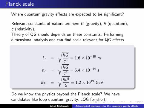
Where quantum gravity effects are expected to be significant?

Relevant constants of nature are here G (gravity), ℏ (quantum),c (relativity).Theory of QG should depends on these constants. Performingdimensional analysis one can find scale relevant for QG effects

lPl =

√

ℏG

c3= 1.6 × 10−35 m

tPl =

√

ℏG

c5= 5.4 × 10−44 s

EPl =

√

ℏc5

G= 1.2 × 1019 GeV

Do we know the physics beyond the Planck scale? We havecandidates like loop quantum gravity, LQG for short.


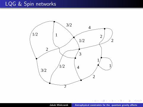
LQG & Spin networks

.

.

..

.

..

..

1/2 1

4

22

2

2

4

1/2

3/2

3

1/2

2

3/2

.1

1


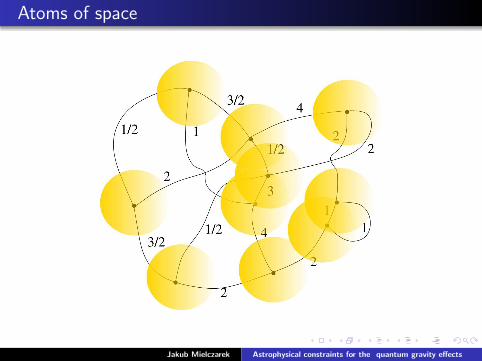
Atoms of space


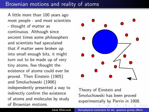
Brownian motions and reality of atoms

A little more than 100 years agomost people - and most scientists- thought of matter ascontinuous. Although sinceancient times some philosophersand scientists had speculatedthat if matter were broken upinto small enough bits, it mightturn out to be made up of verytiny atoms, few thought theexistence of atoms could ever beproved. Then Einstein (1905)and Smoluchowski (1906)independently presented a way toindirectly confirm the existenceof atoms and molecules by studyof Brownian motions.

Theory of Einstein andSmoluchowski has been provedexperimentally by Perrin in 1908.


Observational status of QG

A main obstacle in formulating quantum theory of gravitationalinteractions is the lack of any empirical clue. For now there is noempirical evidence of quantum gravity. Since quantum gravityeffects are expected to be significant at the energies approaching1019 GeV, direct experimental probing becomes inaccessible.Therefore alternative methods of investigation ought to be takeninto account. The most promising involve observations of thecosmos.

LHC reach 14 TeV (presently up to 1 TeV at Tevatron) while weneed 1016 TeV (Planck energy). We never reach it with thepresent generation of accelerators.

It is like probing atomic structure with Earth size resolutiondevices!

Other possibilities? → ”Indirect methods”


Indirect methods

Because we are not able to create sufficient conditions in thelaboratories on Earth, we have to look for them in space.

Cosmology

LQG → Big Bounce → primordial perturbations → CMB

Relic gravitational waves → B-type polarization of CMB

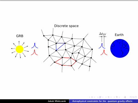
Violation of Lorentz Invariance

Modified dispersion relation → short-duration GRB

Threshold anomalies → effects on GKZ cutoff

Gravitational collapse

Threshold mass for black holes → cutoff on the smallprimordial black holes?


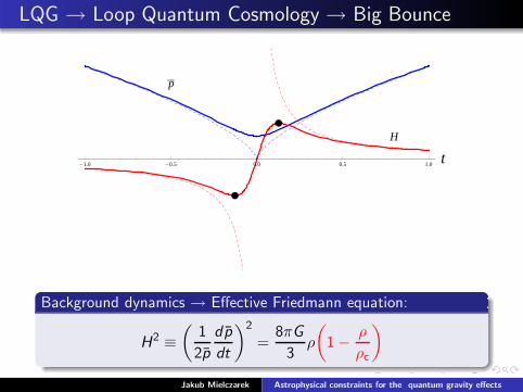
LQG → Loop Quantum Cosmology → Big Bounce

p��

H

-1.0 -0.5 0.0 0.5 1.0 t

Background dynamics → Effective Friedmann equation:

H2 ≡

(

1

2p

d p

dt

)2

=8πG

3ρ

(

1 −ρ

ρc

)


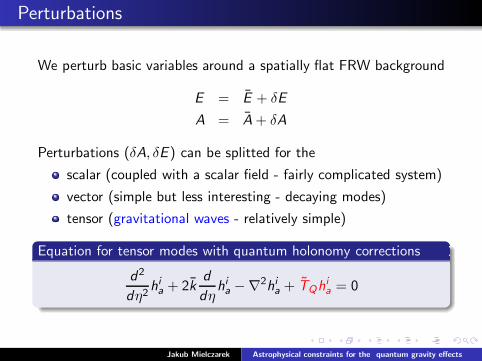
Perturbations

We perturb basic variables around a spatially flat FRW background

E = E + δE

A = A + δA

Perturbations (δA, δE ) can be splitted for the

scalar (coupled with a scalar field - fairly complicated system)

vector (simple but less interesting - decaying modes)

tensor (gravitational waves - relatively simple)

Equation for tensor modes with quantum holonomy corrections

d2

dη2hia + 2k

d

dηhia −∇2hi

a + TQhia = 0


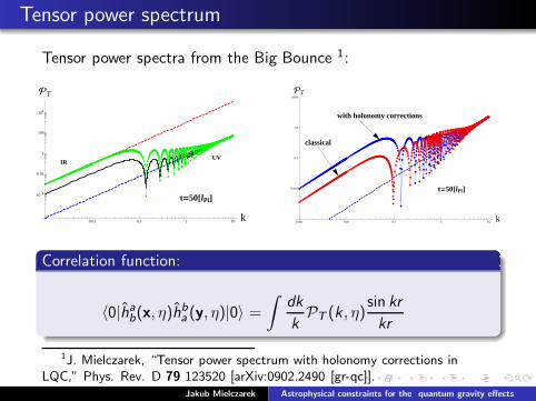
Tensor power spectrum

Tensor power spectra from the Big Bounce 1:

IRUV

t=50@lPlD

0.01 0.1 1 10 k

10-4

0.01

1

100

104

PT

classical

with holonomy corrections

t=50@lPlD

0.001 0.01 0.1 1 10 k

0.001

0.1

10

1000

PT

Correlation function:

〈0|hab(x, η)hb

a (y, η)|0〉 =

∫

dk

kPT (k, η)

sin kr

kr

1J. Mielczarek, “Tensor power spectrum with holonomy corrections inLQC,” Phys. Rev. D 79 123520 [arXiv:0902.2490 [gr-qc]].


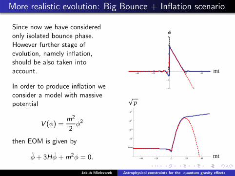
More realistic evolution: Big Bounce + Inflation scenario

Since now we have consideredonly isolated bounce phase.However further stage ofevolution, namely inflation,should be also taken intoaccount.

In order to produce inflation weconsider a model with massivepotential

V (φ) =m2

2φ2

then EOM is given by

φ + 3Hφ + m2φ = 0.

-40 -20 20 40 mt

-2

-1

1

2

3

4

Φ

-40 -20 0 20 40 mt

1000

109

1015

1021

1027

�!!!!p��


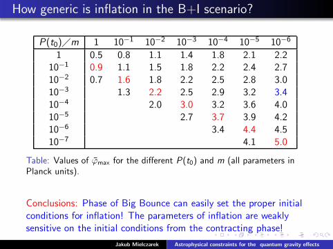
How generic is inflation in the B+I scenario?

P(t0)�m 1 10−1 10−2 10−3 10−4 10−5 10−6

1 0.5 0.8 1.1 1.4 1.8 2.1 2.210−1 0.9 1.1 1.5 1.8 2.2 2.4 2.710−2 0.7 1.6 1.8 2.2 2.5 2.8 3.010−3 1.3 2.2 2.5 2.9 3.2 3.410−4 2.0 3.0 3.2 3.6 4.010−5 2.7 3.7 3.9 4.210−6 3.4 4.4 4.510−7 4.1 5.0

Table: Values of ϕmax for the different P(t0) and m (all parameters inPlanck units).

Conclusions: Phase of Big Bounce can easily set the proper initialconditions for inflation! The parameters of inflation are weaklysensitive on the initial conditions from the contracting phase!


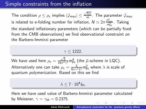
Simple constraints from the inflation

The condition ρ ≤ ρc implies |ϕmax| ≤√

2ρc

m. The parameter ϕmax

is related to e-folding number for inflation, N ≃ 2πϕ2

max

m2Pl

. Taking

the standard inflationary parameters (which can be partially fixedfrom the CMB observations) we find observational constraint onthe Barbero-Immirzi parameter

γ ≤ 1222.

We have used here ρc =√

316π2γ3 m

4Pl (the µ-scheme in LQC).

Alternatively one can take ρc = 38πγ2λ2 m

2Pl where λ is scale of

quantum polymerization. Based on this we find

λ ≤ 7 · 104lPl.

Here we have used value of Barbero-Immirzi parameter calculatedby Meissner, γ = γM = 0.2375.


Towards testing the quantum cosmology models

Work in collaboration with Micha l Kamionka, Aleksandra Kurekand Marek Szyd lowski.

The standard inflationary spectrum is parametrised in thepower-law form

P1(k) = As

(

k

k0

)ns−1

.

The modifications due to the Big Bounce can be introduced by theadditional prefactor ∆(k, k∗). Then power spectrum takes the form

P2(k) = ∆(k, k∗)As

(

k

k0

)ns−1

.


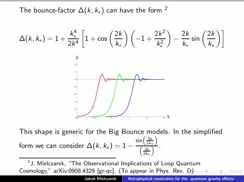
The bounce-factor ∆(k, k∗) can have the form 2

∆(k, k∗) = 1 +k4∗

2k4

[

1 + cos

(

2k

k∗

)(

−1 +2k2

k2∗

)

−2k

k∗sin

(

2k

k∗

)]

0.001 0.01 0.1 1 10 100 k

0.2

0.4

0.6

0.8

1.0

1.2

1.4

D

This shape is generic for the Big Bounce models. In the simplified

form we can consider ∆(k, k∗) = 1 −sin

“

3k2k∗

”

“

3k2k∗

” .

2J. Mielczarek, “The Observational Implications of Loop QuantumCosmology,” arXiv:0908.4329 [gr-qc]. (To appear in Phys. Rev. D)


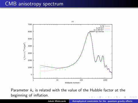
CMB anisotropy spectrum

0

1000

2000

3000

4000

5000

6000

7000

1 10 100 1000

T0

2l(

l+1

) C

lTT/2

π [µ

K2 ]

Multipole moment l

TT

k*=0k*=5*10-4

k*=1.65*10-4

WMAP 5yr binned

Parameter k∗ is related with the value of the Hubble factor at thebeginning of inflation.


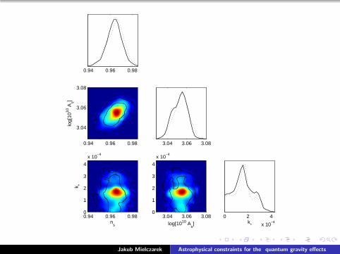
0.94 0.96 0.98

3.04 3.06 3.08

0 2 4

x 10−4k

*

log[

1010

As]

0.94 0.96 0.98

3.04

3.06

3.08

ns

k *

0.94 0.96 0.980

1

2

3

4

x 10−4

log[1010 As]

3.04 3.06 3.080

1

2

3

4

x 10−4


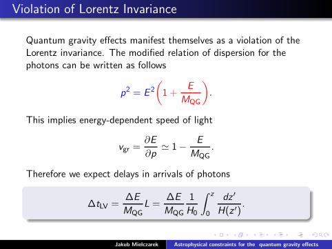
Violation of Lorentz Invariance

Quantum gravity effects manifest themselves as a violation of theLorentz invariance. The modified relation of dispersion for thephotons can be written as follows

p2 = E 2

(

1 +E

MQG

)

.

This implies energy-dependent speed of light

vgr =∂E

∂p≃ 1 −

E

MQG

.

Therefore we expect delays in arrivals of photons

∆tLV =∆E

MQG

L =∆E

MQG

1

H0

∫ z

0

dz ′

H(z ′).


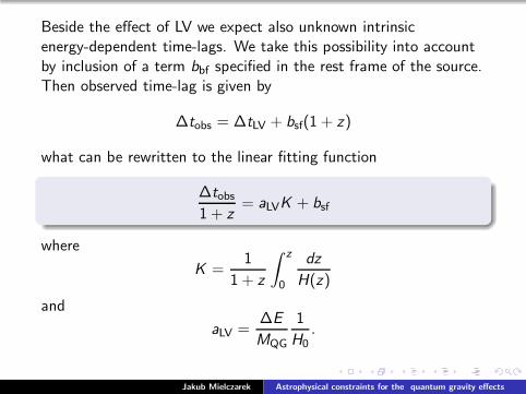
Beside the effect of LV we expect also unknown intrinsicenergy-dependent time-lags. We take this possibility into accountby inclusion of a term bbf specified in the rest frame of the source.Then observed time-lag is given by

∆tobs = ∆tLV + bsf(1 + z)

what can be rewritten to the linear fitting function

∆tobs

1 + z= aLVK + bsf

where

K =1

1 + z

∫ z

0

dz

H(z)

and

aLV =∆E

MQG

1

H0.


-0.2

-0.1

0

0.1

0.2

0.3

0.4

0.15 0.2 0.25 0.3 0.35 0.4

K

∆t/(1

+z)

HETE

BATSE

SWIFT

0.045 0.05 0.055 0.06 0.065 0.07 0.075 0.08−0.24

−0.22

−0.2

−0.18

−0.16

−0.14

bsf

a LV

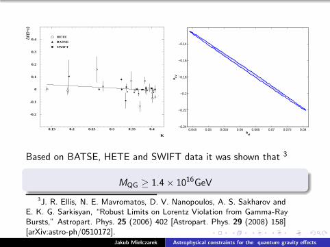
Based on BATSE, HETE and SWIFT data it was shown that 3

MQG ≥ 1.4 × 1016GeV

3J. R. Ellis, N. E. Mavromatos, D. V. Nanopoulos, A. S. Sakharov andE. K. G. Sarkisyan, “Robust Limits on Lorentz Violation from Gamma-RayBursts,” Astropart. Phys. 25 (2006) 402 [Astropart. Phys. 29 (2008) 158][arXiv:astro-ph/0510172].


In 2005, MAGIC recorded VHE γ−ray flares of Mkn 501(z=0.034). Based on these observations it was shown that 4

MQG ≥ 0.21 × 1018GeV

In 2006, HESS observed a giant outburst of the blazar PKS2155-304 (z=0.116). Based on these observations it was shownthat 5

MQG ≥ 0.72 × 1018GeV

4J. Albert et al. [MAGIC Collaboration and Other ContributorsCollaboration], “Probing quantum gravity using photons from a flare of theactive galactic nucleus Markarian 501 observed by the MAGIC telescope,”Phys. Lett. B 668 (2008) 253 [arXiv:0708.2889 [astro-ph]].

5J. Bolmont, R. Buhler, A. Jacholkowska and S. J. Wagner [the H.E.S.S.Collaboration], “Search for Lorentz Invariance Violation effects with PKS2155-304 flaring period in 2006 by H.E.S.S,”arXiv:0904.3184 [gr-qc].


astrophysical constraints for the quantum gravity eﬀectsquantcosmo.ncbj.pl/seminar/mielczarek...

Documents