Asymmetry of Technical Analysis and Market Price Volatility

Min Zheng, Duo Wang, Xue-zhong He

Corresponding author: Min Zheng Organisation: School of Finance and Economics, University of Technology, Sydney, Australia School of Mathematical Sciences, Peking University, China Post address: School of Finance and Economics, University of Technology, Sydney, PO Box 123, Broadway NSW 2007, Australia

Email: min.zheng@uts.edu.au

Tel: +61 2 9514 7762

Fax: +61 2 9514 7711

Research areas: Nonlinear financial dynamics, behaviour finance and asset pricing

Duo Wang Organisation: School of Mathematical Sciences, Peking University, China Post address: School of Mathematical Sciences, Peking University, China, 100871 Email: duo_wang@pku.edu.cn

Tel: +86 10 62755548

Fax: +86 10 62751801

Research areas: Nonlinear dynamics and financial mathematics

Xue-zhong He Organisation: School of Finance and Economics, University of Technology, Sydney, Australia Post address: School of Finance and Economics, University of Technology, Sydney, PO Box 123, Broadway NSW 2007, Australia

Email: tony.he-1@uts.edu.au

Tel: +61 2 9514 7726

Fax: +61 2 9514 7711 Research areas: Financial market modelling, heterogeneous expectations and learning, nonlinear economic dynamics and bounded rationality, behaviour finance and asset pricing

The authors are very grateful to the financial support from the Natural Science Foundation of China (10571003, 10871005). They also thank the referees very much for their very careful reviewing and beneficial suggestions.

Asymmetry of Technical Analysis and Market Price

Volatility

Abstract

Within the framework of heterogeneity and bounded rationality, this papermodels the financial market as an interaction of two types of boundedly rationalinvestors—fundamentalists and chartists. The model is characterised by a nonlin-ear dynamical system. Applying stability and bifurcation theory, we examine thedynamics of the market price and market behaviour. It is found that investors’behaviour, in particular the asymmetric beliefs of the chartists and the interactionof the two types of investors play a very important role in explaining the marketvolatility. Numerical simulations of the corresponding stochastic model demon-strate that the model is able to generate the stylised facts, including volatilityclustering, high kurtosis, and the long-range dependence of asset return observedin financial markets.

Keywords: price fluctuation, bounded rationality, asymmetrical beliefs, stability,bifurcation

JEL: C62, D53, E32, E44, G12

1

1 Introduction

Volatility is an inherent characteristic of financial markets. It provides investors

opportunities for obtaining high excess returns which are however associated with high

risk in general. With the development and diversity of financial markets, it becomes more

important and interesting to understand market volatility and its underlying market

mechanism.

The traditional financial theory developed since the 1950s is based on the assumptions

of the rational expectation and the representative agent. Based on the assumptions, asset

prices are the outcome of the market interaction of utility maximising agents who use

rational expectations when forming their expectations about future market outcomes.

Preferences of agents are assumed to satisfy conditions that enable the mass of investors

to be considered as a single representative agent. Since agents are rationally impounding

all relevant information into their trading decisions, the movement of prices is assumed

to be perfectly random and hence exhibit the so-called random walk behaviour. Namely,

market prices do not change if there is no new information, see Fama (1965). These are

the classical rational expectation and efficient market hypothesis. This view is important

in empirical finance, see Sargent (1993). It is also the basis of the stochastic price

mechanisms assumed in many of the key theoretical models in finance, such as the optimal

portfolio theory that has developed out of the work of Markowitz (1952) and Merton

(1971), the static and dynamic capital asset pricing model of Sharpe (1964), Lintner

(1965), Mossin (1966) and Merton (1973), and models for the pricing of contingent claims

beginning with the work of Black and Scholes (1973). The empirical work represented

by Fama (1976) provided favourable evidence in earlier empirical studies to support the

market efficiency and random walk hypothesis and financial experts and economists have

used the theory to explain observed market prices.

There appears a range of abnormal phenomena in financial markets, however, which

cannot be explained within the framework of the traditional financial theory since the

1980s. They include equity premium puzzle (the anomalously higher historical real re-

turns of stocks over government bonds), excess volatility (excess volatility of stock price

cannot be explained by rational fundamental value adjustment based on random news),

volatility clustering (large changes tend to be followed by large changes, of either sign,

and small changes tend to be followed by small changes), long memory (returns per se

are unpredictable but their absolute and squared values have significant autocorrelation

with a hyperbolic decay structure), popularity of technical analysis (such as simple mov-

ing average, momentum strategy and percentage retracement) and herd behaviour (the

tendency for individuals to mimic the rational or irrational actions of a larger group).

In addition, the return distribution displays characteristics which are different from nor-

mal distribution underlying the traditional finance theory, such as skewness, fat tail and

higher kurtosis. Certainly the 1987 crash has been well researched but so far there is no

satisfactory explanation of what was the “news event” that triggered such a large market

2

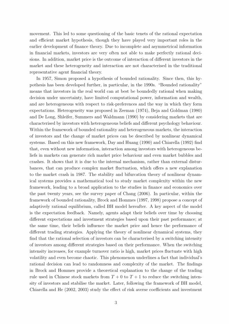
movement. This led to some questioning of the basic tenets of the rational expectation

and efficient market hypothesis, though they have played very important roles in the

earlier development of finance theory. Due to incomplete and asymmetrical information

in financial markets, investors are very often not able to make perfectly rational deci-

sions. In addition, market price is the outcome of interaction of different investors in the

market and these heterogeneity and interaction are not characterised in the traditional

representative agent financial theory.

In 1957, Simon proposed a hypothesis of bounded rationality. Since then, this hy-

pothesis has been developed further, in particular, in the 1990s. “Bounded rationality”

means that investors in the real world can at best be boundedly rational when making

decision under uncertainty, have limited computational power, information and wealth,

and are heterogeneous with respect to risk-preferences and the way in which they form

expectations. Heterogeneity was proposed in Zeeman (1974), Beja and Goldman (1980)

and De Long, Shleifer, Summers and Waldmann (1990) by considering markets that are

characterised by investors with heterogeneous beliefs and different psychology behaviour.

Within the framework of bounded rationality and heterogeneous markets, the interaction

of investors and the change of market prices can be described by nonlinear dynamical

systems. Based on this new framework, Day and Huang (1990) and Chiarella (1992) find

that, even without new information, interaction among investors with heterogeneous be-

liefs in markets can generate rich market price behaviour and even market bubbles and

crashes. It shows that it is due to the internal mechanism, rather than external distur-

bances, that can produce complex market fluctuation, which offers a new explanation

to the market crash in 1987. The stability and bifurcation theory of nonlinear dynam-

ical systems provides a mathematical tool to study market complexity within the new

framework, leading to a broad application to the studies in finance and economics over

the past twenty years, see the survey paper of Chang (2006). In particular, within the

framework of bounded rationality, Brock and Hommes (1997, 1998) propose a concept of

adaptively rational equilibrium, called BH model hereafter. A key aspect of the model

is the expectation feedback. Namely, agents adapt their beliefs over time by choosing

different expectations and investment strategies based upon their past performance; at

the same time, their beliefs influence the market price and hence the performance of

different trading strategies. Applying the theory of nonlinear dynamical systems, they

find that the rational selection of investors can be characterised by a switching intensity

of investors among different strategies based on their performance. When the switching

intensity increases, for example turnover ratio is high, market prices fluctuate with high

volatility and even become chaotic. This phenomenon underlines a fact that individual’s

rational decision can lead to randomness and complexity of the market. The findings

in Brock and Hommes provide a theoretical explanation to the change of the trading

rule used in Chinese stock markets from T + 0 to T + 1 to reduce the switching inten-

sity of investors and stabilise the market. Later, following the framework of BH model,

Chiarella and He (2002, 2003) study the effect of risk averse coefficients and investment

3

strategies of investors in different market scenarios on market prices. Hommes, Huang

and Wang (2005) demonstrate the robustness of BH model. Chiarella, He and Hommes

(2006) extend BH model to study the dynamic behaviour of moving average rules and

explain various market price phenomena including temporary bubbles, sudden market

crashes, and price switching between different levels. Gaunersdorfer, Hommes and Wa-

gener (2007) try to provide an explanation in the generating mechanism on the volatility

clustering based on BH model. Using empirical data, Boswijk, Hommes and Manzan

(2007) and Gaunersdorfer and Hommes (2007) test the explanation power of BH model

to real markets by applying some statistic methods. Recently, He and Li (2007b, 2008)

use a simpler market fraction model to describe the relationship between the phenomena

and statistic characteristics observed in real markets and the dynamic behaviour of the

underlying deterministic model, showing that the model is able to generate many stylised

facts (especially long memory) which is difficult to explain in the traditional finance the-

ory. They provide an explanation successfully on the generating mechanism from the

viewpoint of dynamics. We refer the reader to the survey paper of Hommes (2006) for the

development in this literature. In another survey paper, Chiarella, Dieci and He (2009)

provide a comprehensive summary about how to use the method of nonlinear dynamical

systems to study the market price changes within the framework of heterogeneous belief

and bounded rationality. In addition, there is a great contribution in artificial financial

markets to explore complex phenomena in real markets, for example, Lettau (1997),

LeBaron, Arthur and Palmer (1999) and Chen and Yeh (2001). We refer the reader to

the surveys of LeBaron (2006) and Chen (2007) for the development in this literature.

All the literature has demonstrates that the models are able to describe some stylised

phenomena observed in financial markets, such as volatility persistence and fat tail, and

provide insight into the important role of investors’ heterogeneity and bounded rational-

ity in explaining market volatility. This demonstrates that nonlinear dynamical system

as a mathematical tool provides a great potential to the study of this new framework.

More recently, the method has been extended to the study in exchange rate markets and

macroeconomics, see, for example Chiarella, He and Zheng (2009). In this paper, we

seek to use the framework of heterogeneous beliefs and bounded rationality to study the

impact of asymmetric belief in technical analysis on market volatility.

In the current literature of heterogeneous agent models, it is usually assumed that

heterogeneous beliefs of agents are either linear or nonlinear but symmetric, meaning

that investors have symmetric beliefs to changes of market prices in different market

situations. However, in real markets, investors can have different views on the market

condition and react differently to ups and downs of market prices. In other words, there

exists an asymmetric effect in financial markets and investors can have asymmetric views

on price signals in different market situations. For example, Veronesi (1999) shows that

in equilibrium, investors’ willingness to hedge against changes in their own “uncertainty”

on the true state makes stock price overreact to bad news in good times and underreact to

good news in bad times. Lu and Xu (2004) find that the asymmetric market reaction in

4

the Chinese stock markets is different from other countries. Using EGARCH model, they

test asymmetric characteristics of the Chinese stock markets in bullish/bearish states

and explain the “Matthew Effect” from aspects of anticipation, structure, psychology

and trading mechanism. Based on the data from the Shanghai Stock Exchange, He and

Li (2007a) analyse the asymmetric characteristics of return and volatility in different

market trends and find that there is obvious difference of mean-reverting between bull

and bear markets and rational expectation hypothesis does not hold. Hirshleifer (2001)

gives a nice survey on investor psychology and asset pricing.

The questions are then how to model the asymmetric views of investors and what

is the impact of the asymmetric reaction on market price volatility. An understanding

of these questions hopes to help us to explain complex phenomena in financial mar-

kets. In this paper, within the framework of BH model and Chiarella, He and Hommes

(2006), we introduce an asymmetric belief into one of commonly used technical strate-

gies, namely percentage retracement, and examine the impact of the asymmetric beliefs

of the chartists on the market complexity, in particular, the market price volatility by

using the tools of nonlinear dynamical systems and statistics. By analysing the corre-

sponding deterministic model, we find that the asymmetric beliefs of the chartists to

market price signals play an important role in the deviation of market price from its

fundamental value. In addition, the adaptive behaviour of investors to update their

strategies based on their performance results in herding behaviour and enforces market

volatility. This implies that the bounded rational behaviour of investors is an important

source of market volatility. Therefore, market volatility is the intrinsic characteristics of

the development of financial markets.

The paper is organised as follows. Section 2 sets up an asset pricing model of the fun-

damentalists and chartists who have asymmetric beliefs about market. Mathematically,

the model is described by a high-dimensional stochastic nonlinear dynamical system.

To help our understanding, we focus more on the economic intuition of the analysis of

the model. Following the standard approach in nonlinear dynamical systems, Section 3

applies the stability and bifurcation theory to analyse the corresponding deterministic

model without random perturbations and to examine the stability and complexity of

the model. This analysis provides a theoretic foundation for the analysis of the orig-

inal stochastic model. In Section 4, we introduce market noise and assume that the

fundamental price follows a stochastic process. By numerical simulations, we explore

the impact of the asymmetric beliefs and the random perturbations on market price.

Further economic discussion and a conclusion are included in Section 5. To focus on the

economic intuition, rather than the technical details, of the model, we leave the mathe-

matical proofs of the theoretic results in the appendix. We hope this paper can provide

a new framework and approach for the Chinese researchers to study qualitatively and

quantitatively financial market behaviour and help us to improve our understanding of

market operation and to manage the risk, especially in the currently globally financial

crisis.

5

2 Model

Consider a market with one risky asset (for instance stock, index or managed fund)

and one risk free asset. Let Pt denote the price (ex dividend) per share of the risky

asset at time t, and let yt be the stochastic dividend process of the risky asset. The

risk free asset is perfectly elastically supplied at return r. In our paper, we assume the

risky asset price is determined by a market maker who adjusts the market price based on

the imbalance between demand and supply. That is, when demand exceeds supply, the

price goes up and otherwise the price goes down. Different from the rational expectation

and representative agent hypothesis in the traditional theory, we assume that investors

have heterogeneous beliefs and they are bounded rational. The heterogeneous beliefs are

described by different expectations about future price, while the bounded rationality is

captured by different trading strategies based on different beliefs and adaptive switching

among different strategies based on their performance. Heterogeneous expectations have

been found in empirical studies, especially in exchange rate markets, and have been used

widely in modelling financial market behaviour. In line with Chiarella, He and Hommes

(2006), we group different types of investors by their beliefs and the risky asset price can

be set period by period upon the aggregate excess demand Dt, which is given by

Dt =∑q∈Q

nq,tDqt ,

where Q represents the set of types of investors, Dqt (q ∈ Q) is the excess demand of type

q trader at time t, nq,t is the market fraction of type q traders at time t. The number

of investors can be arbitrary but the fractions of all types of investors must satisfy∑q∈Q nq,t = 1. Here it is necessary to point out that it is usually assumed in traditional

models that the market maker adjusts the risky asset price in absolute amount based

on the aggregate excess demand, that is Pt+1 − Pt = P(Dt). Under this mechanism, the

market price can be negative; also, when there is a same excess demand for the risky

asset with different fundamental prices, the stock price evolution is the same, which is

not realistic. In our model, we adopt the relative price, instead of the absolute price,

adjustment mechanism of the market maker. Namely,

Pt+1 − Pt

Pt

= S(Dt) = S(∑

q∈Q

nq,tDqt

), (1)

where S(x) is a monotonically increasing function, which models the function of price

adjustment by the market maker in market maker scenario. A consideration of wealth

constraint and the stylising role of the market maker implies that the function S(x)

is usually assumed to be an S-shaped function, see Figure 1. For simplicity, we take

S(x) = k tanh(hx), where 0 < k < 1, h > 0. Therefore, when Dt > 0, there exists

an excess demand in the market which pushes the price up, namely Pt+1 > Pt. When

Dt < 0, there exists an excess supply in the market, pushing the price down Pt+1 < Pt.

6

In addition, under the assumption of S(x) = k tanh(hx),

∣∣∣∣∣Pt+1 − Pt

Pt

∣∣∣∣∣ < k.

Hence, k represents the maximum up and low limits of the risky asset price, like the 10%

up and low price limits used in the Chinese stock markets. The parameter µ = S ′(0) = kh

measures the adjustment speed near zero excess demand, which captures the future price

change when the excess demand is close to zero. For an economic explanation of the S-

shaped function, we refer the reader to Chiarella (1992) and Chiarella, Dieci and Gardini

(2002).

Insert Figure 1 here

In financial markets, investment strategies capturing different price expectations are

used widely, among which, two types of investors are especially common, fundamentalists

who use fundamental analysis and chartists who use various price indices of the future

price trend. For simplicity, we assume throughout this paper that there are only two

types of traders, fundamentalists and chartists, that is Q = {fundamentalists, chartists}(in brief Q = {f, c}). Their trading strategies and excess demand functions are specified

in the following discussion.

Fundamentalists–The fundamentalists are assumed to know the fundamental infor-

mation of the risky asset. They use the fundamental analysis and believe that the market

price can deviate from its fundamental value, but in long run, it will converge to the

neighborhood of the fundamental value. Therefore, the fundamentalists focus on the

long-run change of the risky asset price. We assume that the fundamentalists know the

fundamental price of the risky asset and their excess demand depends on the deviation

of the market price from the fundamental value. At time t, without constraint in wealth,

their excess demand Dft is assumed to be proportional to the difference between the

fundamental price Ft and the market price Pt, namely

Dft = α(Ft − Pt),

where α > 0 is the reaction coefficient of the fundamentalists, which represents the mean-

reverting beliefs of the fundamentalists. When Ft > Pt, the fundamentalists believe that

the risky asset is undervalued and so they take a long position. Contrarily, the price is

regarded as overvaluation and so they take a short position. Moreover, the more price

deviation, the more excess demand. In general, from the viewpoint of the market price

containing the information of the fundamental, the fundamentalists play an active role

in stabilising markets. However, when their adjustment speed (α) is too high, they can

make the market unstable. The phenomena of the stability and instability induced by

the fundamentalists’ over-adjustment will be discussed in detail.

7

Chartists–The chartists believe that the charting signals from past prices contain

some information about the future change of the price of the risky asset. They prefer

cheaper thumb strategies, such as simple moving average, percentage retracement, mo-

mentum, Fibonacci studies, and other popular technical methods in financial markets,

see Murphy (2004). In our paper, we mainly seek to analyse the effect of percentage

retracement (PR). A retracement is a countertrend move. The retracement is based on

the thought that prices will reverse or “retrace” a portion of the previous movement

before resuming their underlying trend in the original direction. For example, 33%, 50%

and 66% retracement rates are well known as illustrated in Figure 2. In particular, when

the chartists believe 50% retracement, when the short down-adjustment of the market

price during the rising price trend does not cross the line of 50% PR, the chartists believe

that the price down-trend has not been formed, the market price is just in a temporary

adjustment and it will go up after the adjustment and they hence take a long position

on the risky asset; otherwise they believe that the price down-trend is doomed and the

rising price phase is over, so they take a short position on the risky asset, see Figure

2(a). Similarly, the price up-adjustment case is shown in Figure 2(b). It shows that the

chartists focus on the short-term change of the risky asset price in making their invest-

ment decision. This short-term investment behaviour is one of the sources of market

instability, especially when there is an instantaneous big shock in the market.

Insert Figure 2 here

The percentage retracement strategy of the chartists can therefore be expressed by

the weighted historical prices, that is,

Pt = (1− ω)Pt−1 + ωPt−2,

which captures the expected price of the chartists, where ω ∈ [0, 1] represents the coef-

ficient of the retracement strategy. In particular, if ω = 50%, Pt is the simple moving

average of length 2. ω = 33% and 66% respectively represent the 33% and 66% retrace-

ment strategies. A trading signal to trade for the chartists is defined as the difference1

δt between the current price Pt and the expectation price Pt, that is δt = Pt− Pt. When

δt > 0, the chartists believe that the price is in a rising trend and they hence take a

long position; otherwise, they take a short position. Mathematically, this strategy of the

chartists can be written as

Dct = g(δt).

Usually g is a monotonically increasing function of trading signals. Considering a wealth

constraint for the chartists, g is usually assumed to be an S-shaped function, for example

g(x) = u tanh(vx)(u > 0, v > 0). Note that under the assumption, g(·) is a symmetric

and monotonically increasing function and limx→±∞

|g(x)| = u < ∞. It means that the

chartists’ views to positive and negative trading signals are symmetric and the chartists

8

are cautious but not very cautious when the price difference δt is large (either positive

or negative). In contrast, empirical analysis in Veronesi (1999) and Lu and Xu (2004)

show that investors have asymmetric views to market information in financial markets.

In addition, when the market price is far away from the level indicated by the price

trend, the chartists become cautious. In this paper, we consider the chartists who have

different views on the market, for instance, they prefer buying/selling to selling/buying in

bullish/bearish markets facing the same price deviation δt; they buy/sell more/smaller

in bullish markets compared with bearish markets. They are cautious for large price

rise or fall. These behaviour assumptions imply that g satisfies the following general

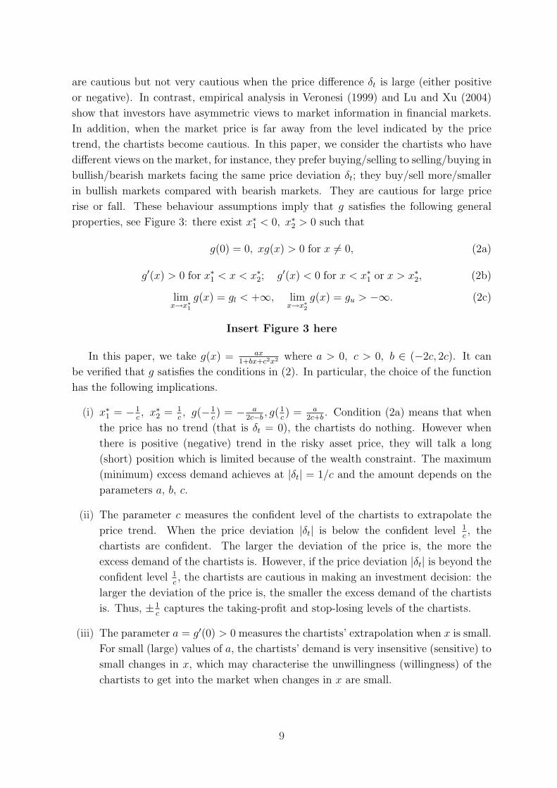
properties, see Figure 3: there exist x∗1 < 0, x∗2 > 0 such that

g(0) = 0, xg(x) > 0 for x 6= 0, (2a)

g′(x) > 0 for x∗1 < x < x∗2; g′(x) < 0 for x < x∗1 or x > x∗2, (2b)

limx→x∗1

g(x) = gl < +∞, limx→x∗2

g(x) = gu > −∞. (2c)

Insert Figure 3 here

In this paper, we take g(x) = ax1+bx+c2x2 where a > 0, c > 0, b ∈ (−2c, 2c). It can

be verified that g satisfies the conditions in (2). In particular, the choice of the function

has the following implications.

(i) x∗1 = −1c, x∗2 = 1

c, g(−1

c) = − a

2c−b, g(1

c) = a

2c+b. Condition (2a) means that when

the price has no trend (that is δt = 0), the chartists do nothing. However when

there is positive (negative) trend in the risky asset price, they will talk a long

(short) position which is limited because of the wealth constraint. The maximum

(minimum) excess demand achieves at |δt| = 1/c and the amount depends on the

parameters a, b, c.

(ii) The parameter c measures the confident level of the chartists to extrapolate the

price trend. When the price deviation |δt| is below the confident level 1c, the

chartists are confident. The larger the deviation of the price is, the more the

excess demand of the chartists is. However, if the price deviation |δt| is beyond the

confident level 1c, the chartists are cautious in making an investment decision: the

larger the deviation of the price is, the smaller the excess demand of the chartists

is. Thus, ±1c

captures the taking-profit and stop-losing levels of the chartists.

(iii) The parameter a = g′(0) > 0 measures the chartists’ extrapolation when x is small.

For small (large) values of a, the chartists’ demand is very insensitive (sensitive) to

small changes in x, which may characterise the unwillingness (willingness) of the

chartists to get into the market when changes in x are small.

9

(iv) The parameter b measures the asymmetry of the chartists’ response to changes of

x. For b = 0, the chartists’ long and short positions are symmetric with respect to

the change of x. However, for b 6= 0, the position of the chartists for positive and

negative information is not symmetric. This means that the chartists have different

views towards the market. The phenomenon is called the asymmetric effect. In

particular, when b < 0, we have a2c+b

> a2c−b

and the chartists have a bullish view

on the market. Otherwise, when b > 0, a2c+b

< a2c−b

and the chartists have a bearish

view on the market. We call b the bull-bear coefficient, in brief B-coefficient2.

(v) The function satisfies limx→±∞

g(x) = 0, meaning that when the price difference x

between the current price and the expectation price trend of the chartists is getting

far away, the chartists become cautious and reduce their demand.

We have quantitatively introduced the heterogeneous beliefs of the investors and

their rational investment strategies guided by their beliefs. Now we turn to bounded

rationality of the investors based on the adaptive behaviour of the investors.

Fitness Measure and Fraction Evolution–At time t, the fitness measure πq,t(q = f, c)

of type q traders can be defined as their realised net profit:

πq,t = (Pt + yt −RPt−1)Dqt−1 − Cq,

where R = 1 + r, Cq ≥ 0 is the transaction cost of type q trader. Since fundamental

information is expensive, the cost for the fundamentalists is more than that for the

chartists, implying that C = Cf−Cc ≥ 0. More generally, one can introduce accumulated

performance measure by considering a weighted average of the net realised profit and

past performance as follows:

Uq,t = πq,t + ηUq,t−1, (3)

where the parameter η ∈ [0, 1) represents the memory of the accumulated fitness func-

tion.

Similarly to Brock and Hommes (1997, 1998) and Chiarella, He and Hommes (2006),

the market fraction nq,t follows the discrete choice probability

nq,t =eβUq,t

Nt

,

where Nt =∑

q∈Q eβUq,t and the parameter β(≥ 0) is the switching intensity measuring

how fast the fractions of different type agents in the market switch each other, based

on the performance measure. In particular, for β = ∞, all the investors will choose the

optimal strategy in each period. For a more extensive discussion on the discrete choice

model, we refer to Manski and McFadden (1981) .

10

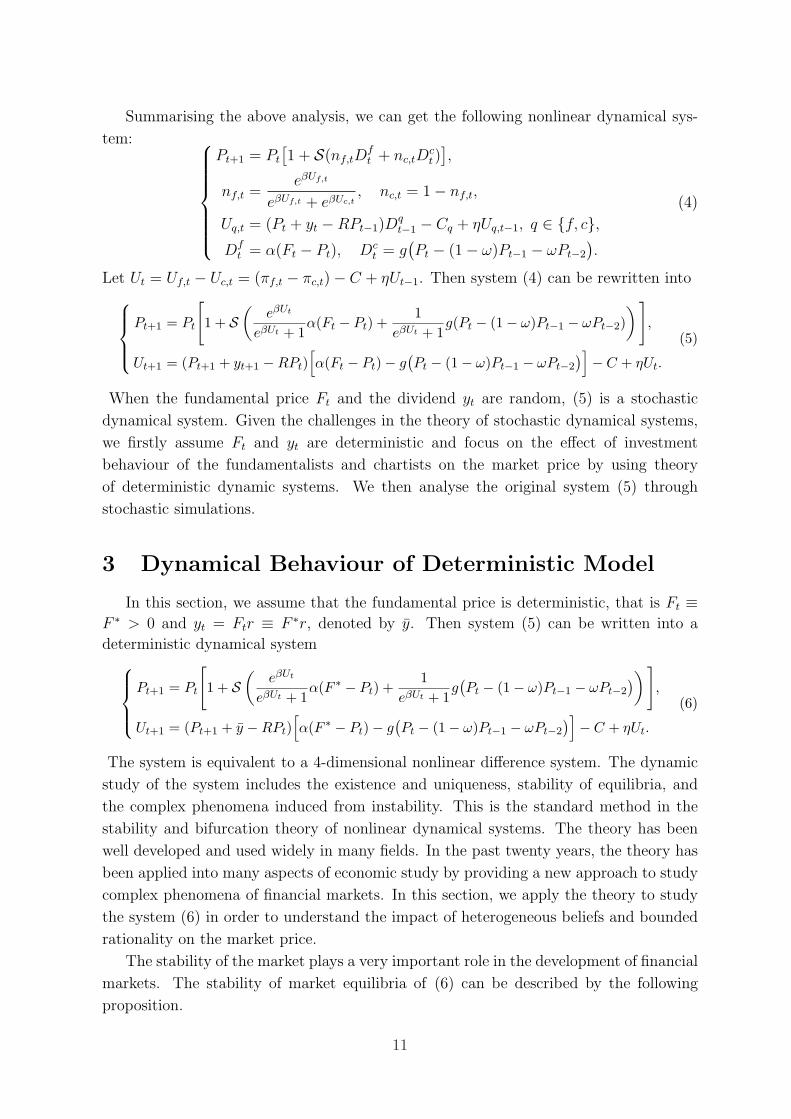
Summarising the above analysis, we can get the following nonlinear dynamical sys-

tem:

Pt+1 = Pt

[1 + S(nf,tD

ft + nc,tD

ct )

],

nf,t =eβUf,t

eβUf,t + eβUc,t, nc,t = 1− nf,t,

Uq,t = (Pt + yt −RPt−1)Dqt−1 − Cq + ηUq,t−1, q ∈ {f, c},

Dft = α(Ft − Pt), Dc

t = g(Pt − (1− ω)Pt−1 − ωPt−2

).

(4)

Let Ut = Uf,t − Uc,t = (πf,t − πc,t)− C + ηUt−1. Then system (4) can be rewritten into

Pt+1 = Pt

[1 + S

(eβUt

eβUt + 1α(Ft − Pt) +

1eβUt + 1

g(Pt − (1− ω)Pt−1 − ωPt−2)) ]

,

Ut+1 = (Pt+1 + yt+1 −RPt)[α(Ft − Pt)− g

(Pt − (1− ω)Pt−1 − ωPt−2

)]− C + ηUt.

(5)

When the fundamental price Ft and the dividend yt are random, (5) is a stochastic

dynamical system. Given the challenges in the theory of stochastic dynamical systems,

we firstly assume Ft and yt are deterministic and focus on the effect of investment

behaviour of the fundamentalists and chartists on the market price by using theory

of deterministic dynamic systems. We then analyse the original system (5) through

stochastic simulations.

3 Dynamical Behaviour of Deterministic Model

In this section, we assume that the fundamental price is deterministic, that is Ft ≡F ∗ > 0 and yt = Ftr ≡ F ∗r, denoted by y. Then system (5) can be written into a

deterministic dynamical system

Pt+1 = Pt

[1 + S

(eβUt

eβUt + 1α(F ∗ − Pt) +

1eβUt + 1

g(Pt − (1− ω)Pt−1 − ωPt−2

))],

Ut+1 = (Pt+1 + y −RPt)[α(F ∗ − Pt)− g

(Pt − (1− ω)Pt−1 − ωPt−2

)]− C + ηUt.

(6)

The system is equivalent to a 4-dimensional nonlinear difference system. The dynamic

study of the system includes the existence and uniqueness, stability of equilibria, and

the complex phenomena induced from instability. This is the standard method in the

stability and bifurcation theory of nonlinear dynamical systems. The theory has been

well developed and used widely in many fields. In the past twenty years, the theory has

been applied into many aspects of economic study by providing a new approach to study

complex phenomena of financial markets. In this section, we apply the theory to study

the system (6) in order to understand the impact of heterogeneous beliefs and bounded

rationality on the market price.

The stability of the market plays a very important role in the development of financial

markets. The stability of market equilibria of (6) can be described by the following

proposition.

11

Proposition 1 (Existence and Stability of Equilibria) Denote U∗ = − C1−η

, n∗f = eβU∗

eβU∗+1,

n∗c = 1 − n∗f and α := F ∗µn∗fα, a := F ∗µn∗ca. Then for the deterministic dynamical

system (6),

(1) there exist two steady states (P ∗1 , U∗

1 ) = (0, αF ∗y−C1−η

), and (P ∗2 , U∗

2 ) = (F ∗, U∗),

(2) (P ∗1 , U∗

1 ) is unstable for all parameters (a, α, ω),

(3) (P ∗2 , U∗

2 ) is locally asymptotically stable(LAS) for (a, α, ω) ∈ D, where

D =

{(a, α, ω) : 0 < ω ≤ 1, 0 < a <

1ω

, max

{0,

(ωa + 1)((1 + ω)a− 1

)

aω

}< α < 2 + 2a(1− ω);

ω = 0, 0 < a < 1, 0 < α < 2 + 2a

}.

Insert Figure 4 here

Proposition 1 indicates that the system (6) has two steady states. The price of the

first steady state (P ∗1 , U∗

1 ) is zero. This steady state is always unstable. This implies

that an asset with zero price has no value and such asset does not exist in financial

markets. In addition, it also implies that an under-valued asset will recover its value.

This phenomenon is consistent with what we observe in financial markets. The price

of the second steady state (P ∗2 , U∗

2 ) is the fundamental value F ∗ of the risky asset and

we call (P ∗2 , U∗

2 ) the fundamental steady state. The stability of the fundamental steady

state is determined by the parameters ω, a = F ∗µn∗ca and α = F ∗µn∗fα, see Figure 4,

where (a, α) are the adjusted reaction intensities (or called extrapolation rates) of the

fundamentalists and chartists scaled by the fundamental price F ∗, the speed of the price

adjustment µ, and the market fractions, nf and nc. Based on the stable region of the

fundamental steady state in Figure 4(b), we can see that, when the parameters (a, α) are

close to the diagonal, the fundamental steady state is stable; when ω is smaller, (a, α)

need to be closer to the diagonal in order to maintain the stability of the fundamental

steady state. This indicates that the stability of the fundamental steady state can be

maintained when the behaviour between the fundamentalists and chartists are balanced.

Thus, when the beliefs of the two types of investors are very different, especially when the

chartists put more weight to the last price when forming their expectation, the stability

of the fundamental price is hardly maintained and the market price will be driven away

from its fundamental value. In addition, if the up and low limit (k) of the risky asset

price is large, the adjustment parameter (µ) of the price increases and moreover, a and α

become larger so that (a, α) leave the stability region of the fundamental steady state and

(P ∗2 , U∗

2 ) becomes unstable. Hence, an increase in price up and low limit increases the

possibility of the market price deviation from its fundamental value. Thus, by controlling

this limit, the market can be stabilised. This observation supports the policy of limiting

daily price change by up to 10% implemented in the Chinese stock markets since 1996.

12

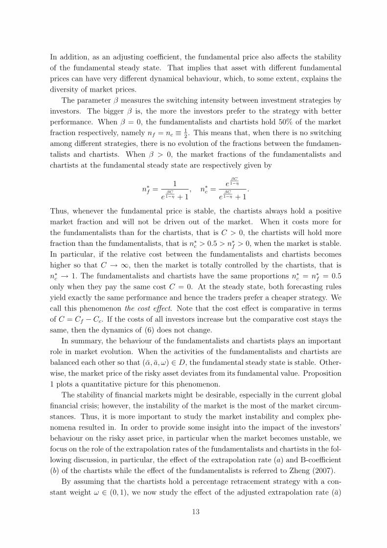
In addition, as an adjusting coefficient, the fundamental price also affects the stability

of the fundamental steady state. That implies that asset with different fundamental

prices can have very different dynamical behaviour, which, to some extent, explains the

diversity of market prices.

The parameter β measures the switching intensity between investment strategies by

investors. The bigger β is, the more the investors prefer to the strategy with better

performance. When β = 0, the fundamentalists and chartists hold 50% of the market

fraction respectively, namely nf = nc ≡ 12. This means that, when there is no switching

among different strategies, there is no evolution of the fractions between the fundamen-

talists and chartists. When β > 0, the market fractions of the fundamentalists and

chartists at the fundamental steady state are respectively given by

n∗f =1

eβC1−η + 1

, n∗c =e

βC1−η

eβC1−η + 1

.

Thus, whenever the fundamental price is stable, the chartists always hold a positive

market fraction and will not be driven out of the market. When it costs more for

the fundamentalists than for the chartists, that is C > 0, the chartists will hold more

fraction than the fundamentalists, that is n∗c > 0.5 > n∗f > 0, when the market is stable.

In particular, if the relative cost between the fundamentalists and chartists becomes

higher so that C → ∞, then the market is totally controlled by the chartists, that is

n∗c → 1. The fundamentalists and chartists have the same proportions n∗c = n∗f = 0.5

only when they pay the same cost C = 0. At the steady state, both forecasting rules

yield exactly the same performance and hence the traders prefer a cheaper strategy. We

call this phenomenon the cost effect. Note that the cost effect is comparative in terms

of C = Cf − Cc. If the costs of all investors increase but the comparative cost stays the

same, then the dynamics of (6) does not change.

In summary, the behaviour of the fundamentalists and chartists plays an important

role in market evolution. When the activities of the fundamentalists and chartists are

balanced each other so that (α, a, ω) ∈ D, the fundamental steady state is stable. Other-

wise, the market price of the risky asset deviates from its fundamental value. Proposition

1 plots a quantitative picture for this phenomenon.

The stability of financial markets might be desirable, especially in the current global

financial crisis; however, the instability of the market is the most of the market circum-

stances. Thus, it is more important to study the market instability and complex phe-

nomena resulted in. In order to provide some insight into the impact of the investors’

behaviour on the risky asset price, in particular when the market becomes unstable, we

focus on the role of the extrapolation rates of the fundamentalists and chartists in the fol-

lowing discussion, in particular, the effect of the extrapolation rate (a) and B-coefficient

(b) of the chartists while the effect of the fundamentalists is referred to Zheng (2007).

By assuming that the chartists hold a percentage retracement strategy with a con-

stant weight ω ∈ (0, 1), we now study the effect of the adjusted extrapolation rate (a)

13

and the asymmetric belief coefficient (b) of the chartists on the market. The stability

of the fundamental steady state depends on the location of the eigenvalues of the char-

acteristic polynomial of the steady state. When all the eigenvalues are located inside

the unit circle, the fundamental steady state is locally asymptotically stable; otherwise,

it becomes unstable. The change from the stability to instability of the fundamental

steady state is determined by the movement of the eigenvalues from the inside to outside

of the unit circle. When the adjusted extrapolation rate of the fundamentalists α satis-

fies 0 < α < 2ω

and the adjusted extrapolation rate of the chartists increases to a∗, there

exists a pair of complex conjugate eigenvalues on the unit circle for the corresponding

characteristic equation, where

a∗ =αω − 1 +

√(αω − 1)2 + 4(ω + ω2)

2(ω + ω2).

Therefore, at a = a∗, the stability of the fundamental steady state is destroyed, leading to

periodic fluctuations or more complex behaviour in (6). This phenomenon is described by

different types of bifurcations in the framework of nonlinear dynamical systems. In our

model, the instability of the fundamental steady state can be induced by either Neimark-

Sacker or Chenciner bifurcations. A Neimark-Sacker bifurcation occurs when changing

parameter of the system leads to a change in the stability of the fixed point, resulting in a

(quasi-)periodic cycle around the fixed point. In this case the market price will fluctuate

(quasi-)periodically around its fundamental value. A Chenciner bifurcation occurs in

the following situation. Near the bifurcation values of the parameters, a locally stable

fixed point is companied by a locally stable (quasi-)periodic cycle around it, and these

two attractors are separated by an unstable (quasi-)periodic cycle. As the parameters

change, the unstable (quasi-)periodic cycle merges together with the fixed point so that

the fixed point becomes unstable and there remains a locally stable (quasi-)periodic cycle.

The appearance of a Neimark-Sacker or Chenciner bifurcation depends on the first and

second Lyapunov coefficients, see Kuznetsov (2004), which are denoted by `1(a, b) and

`2(a, b), respectively. More precisely, we have the following result.

Proposition 2 (Generalised Neimark-Sacker Bifurcation) For fixed ω ∈ (0, 1), we choose

α ∈ (0, 2ω) and assume (1 + ω)a∗ + 1− α 6= 2 cos(2π

q), where q = 1, . . . , 6.

(1) If for any b, `1(a∗, b) 6= 0, then the fundamental steady state undergoes a Neimark-

Sacker bifurcation at a = a∗.

(2) If there exists b∗ such that at b = b∗, `1(a∗, b∗) = 0, ∂`1(a,b)

∂b

∣∣∣a=a∗,b=b∗

6= 0 and

`2(a∗, b∗) 6= 0, then the fundamental steady state undergoes a Chenciner bifurcation

at (a, b) = (a∗, b∗).

Proposition 2 depicts the characteristics of the market price when the fundamental

steady state loses its stability through different bifurcations. In order to understand

14

the dynamical characteristics when the fundamental steady state loses its stability, it

is necessary to calculate the first and second Lyaponov coefficients of (6) at the funda-

mental steady state. By the theorem of central manifold and the normal form theory

of generalised Neimark-Sacker bifurcation, see Kuznetsov (2004), the first and second

Lyapunov coefficients can be calculated by using the Maple program. For convenience

in calculation, we select ω = 0.5, F ∗ = 100, k = 0.1, h = 0.1, α = 1.2, β = 1, η = 0.2,

R = 1.001, C = 0.1 and choose a as the bifurcation parameter, then the Neimark-Sacker

bifurcation point occurs at a∗ ≈ 1.4514 which is independent of the choice of b and c.

For fixed c = 1.2, the type of bifurcations is determined by the first Lyapunov coefficient

satisfying a quadratic function of b ∈ (−2c, 2c)

`1 = 0.1898b2 − 0.0019b− 0.4683. (7)

When b = b∗1 ≈ −1.5660 or b = b∗2 ≈ 1.5759, `1 = 0, ∂`1∂b

∣∣b=b∗1,2

6= 0 and `2(b∗1) ≈ −0.2736,

`2(b∗2) ≈ −0.2721. Therefore, when a = a∗ and b = b∗1,2, the fundamental steady state

undergoes a Chenciner bifurcation. That is,

(i) when b∗1 < b < b∗2, if a < a∗, the fundamental steady state is stable; at a = a∗,the fundamental steady state undergoes a supercritical Neimark-Sacker bifurcation

with `1 < 0; however if a > a∗, the fundamental steady state is unstable and a

stable invariant circle appears around the fundamental steady state;

(ii) when b < b∗1 or b > b∗2, if a < a∗, the fundamental steady state is stable; if a increases

to a∗, there exist a stable fundamental steady state and a stable invariant circle

which are separated by a unstable invariant circle. At a = a∗, the fundamental

steady state undergoes a subcritical Neimark-Sacker bifurcation with `1 > 0. For

a > a∗, the instable invariant circle submerges into the fundamental steady state,

the fundamental steady state loses its stability, and there exists a stable invariant

circle which is far away from the fundamental steady state.

Equation (7) clearly indicates the impact of the asymmetric beliefs of the chartists

on the market price. The change of B-coefficient b affects the first Lyapunov coefficient

and the dynamics of the whole system (6). In particular, when the beliefs are symmetric

(b = 0), we have `1 < 0, meaning that the resulting Neimark-Sacker is supercritical. In

other words, when the extrapolation rate of the chartists increases, the price of the risky

asset fluctuates around its fundamental value and is characterised by a stable invariant

circle. However, when the chartists have asymmetric beliefs (so that b 6= 0), changes of

the intensity of the asymmetric beliefs of the chartists, measured by the B-coefficient,

lead to changing signal of the first Lyapunov coefficient so that `1 becomes positive. In

this case, the Neimark-Sacker bifurcation becomes subcritical, meaning that there exist

two attractors, one is the stable fundamental steady state and one is a stable invariant

circle. Under this circumstance, the price evolution of the system (6) depends on the

initial state. When the initial price is close to its fundamental value, the risky asset

15

price converges to the fundamental value asymptotically; however, when the initial price

is far away from its fundamental value, the risky asset price fluctuates wildly around the

fundamental value. This indicates that the asymmetric beliefs of the chartists is one of

the important sources for the complexity of market price.

Insert Figure 5 here

Figures 5 and 6 illustrate that when the extrapolation rate of the chartists to the price

trend increases, different types of Neimark-Sacker bifurcations occur. In particularly,

Figure 5 displays the bifurcation plot and phase plot when the beliefs of the chartists are

symmetrical, b = 0, to the up and down price signals. We demonstrate that when the

extrapolation rate of the chartists a increases to a∗ ≈ 1.4514, the fundamental steady

state loses its stability and a stable invariant circle around the fundamental steady state

appears and a supercritical Neimark-Sacker bifurcation occurs with the corresponding

first Lyapunov coefficient of `1 = −0.4683 < 0. Consequently, the market price oscillates

in the neighborhood of the fundamental price.

Insert Figure 6 here

However, when the chartists’ beliefs are bullish, for instance b = −1.6, at the bifurca-

tion point a = a∗, the first Lyapunov coefficient of the fundamental steady state is posi-

tive, `1 = 0.0205 > 0. This implies that, when the extrapolation rate of the chartists a

crosses the Neimark-Sacker bifurcation point a∗, the fundamental steady state undergoes

a subcritical Neimark-Sacker bifurcation, leading to the coexistence of two attractors.

More precisely, when the activity of the chartists is very weak so that a = 1.42 < a∗, the

fundamental steady state is stable, see Figure 6(a). When the activity of the chartists

is relatively weak so that a = 1.451 / a∗, then there exist a stable fundamental steady

state and a stable invariant circle which are separated by an unstable invariant circle, as

shown in Figure 6(c). From Figure 6(e), we can see that if the initial price is far away

from its fundamental value, the risky asset price converges to the stable invariant circle

and generates high fluctuations; otherwise, the price converges to its fundamental value.

To sum up, the price behaviour of the risky asset depends on the initial states of the

system.

There is a strikingly simple economic intuition on the coexistence of a stable funda-

mental steady state and a stable invariant circle in our simple evolutionary model when

the chartists have strong bullish beliefs on the market but the extrapolation rate of the

chartists is relatively weakly. When the extrapolation rate of the chartists is weak, the

fundamental steady state will be locally stable, since the extrapolation from the chartists

for prices near the fundamental steady state is not strongly enough for prices to diverge

and the price will therefore converge to the fundamental steady state. However, when

the chartists’ extrapolate rate is weak, an upward price trend far away from the fun-

damental price will be reenforced, making the price to deviate even further away from

16

the fundamental price due to the strong bullish beliefs of the chartists and a large long

position they have. Hence, such a diverging upward price trend is accelerated by the

demand of the chartists until the deviation reaches their threshold confidence level at

which the chartists become cautious. Once the chartists become less confident, they

reduce their long position. At the same time, since the price is also far away from the

fundamental, hence the fundamentalists buy the risky asset at a lower price and sell it

at a higher price. Therefore, the positions held by the fundamentalists and the chartists

are opposite, which slows down the upward price trend and eventually the price trend is

reversed and moves towards the fundamental price. This results in a situation that the

fundamentalists and chartists both are taking the short position, pushing the price down

so that the price will cross the fundamental price and drop further. However, because of

the strong bullish beliefs of the chartists, the downward price trend is slowed down by

relative small short position taken by the chartists. This, together with the pressure of

the long position taken by the fundamentalists, will reverse the price trend and push the

price upwards. By taking a long position along the price trend, the performance of the

chartists becomes better. The adaptive switching mechanism then makes the market

fraction of the chartists increase, resulting in the price overshooting the fundamental

price. This completes a full cycle around the locally stable fundamental steady state, as

illustrated in Figure 7(a). In the whole process, the asymmetric beliefs of the chartists

and their extrapolation to the market signal play very important roles.

Insert Figure 7 here

If the extrapolation rate of the chartists increases beyond the bifurcation point a∗

so that a = 1.46 > a∗, then the fundamental steady state loses its stability, resulting

in the disappearance of the unstable invariant circle which is then submerged into the

fundamental steady state, together with the stable invariant circle, as shown in Figure

6(g). In this case, even when the initial price is close to the fundamental value, the market

price will move away from the fundamental price and fluctuate along the stable invariant

circle. Hence, the overreaction of the chartists increases the fluctuation amplitude of

the market price. In addition, when a Neimark-Sacker or Chenciner bifurcation happens

with the change of some parameters, the size of the invariant circle generated from the

bifurcation will be enlarged with the increase of the parameters. Hence, as a policy

or regulation issues, if the bifurcation parameters, such as the reaction intensity of the

chartists to the price deviation, decrease when the price is in the uptrend along a larger

invariant circle, the trajectory of the price will move from the larger invariant circle to

a smaller one. Although the uptrend may not be changed immediately, the limitation of

the maximum price deviation from the fundamental steady state becomes smaller and

hence the market risk is reduced.

Similarly, when the chartists have the bearish beliefs so that b = 1.6, a subcritical

Neimark-Sacker bifurcation occurs at a = a∗ with the corresponding Lyapunov coefficient

of `1 = 0.0145 > 0, as illustrated in Figure 6(right panel) and Figure 7(b). The difference

17

from the bullish belief case is that the price is below its fundamental value most of time,

see Figure 6(f).

In this section, the complex phenomena induced by the asymmetric beliefs of the

chartists to market signals is examined when the fundamental steady state is unstable.

The application of the bifurcation theory uncovers the intrinsic characteristics of the

complex phenomena. The theoretic analysis in this section provides a guide to the

following numerical simulations of the stochastic model.

4 Stochastic Simulations

In Section 3, under the assumption of the constant fundamental steady state, we

analyse the complex dynamical behaviour of the system (6) with the change of param-

eters. However, in financial markets, the fundamental price usually is not constant but

random, which is affected by international financial markets. In addition, some uncer-

tain factors, such as the arrival of new events or new policies, can also influence the

market. Therefore, the randomness is an important element of financial markets. In this

section we explore the effect of random perturbations on the model by using stochastic

simulations.

Consider the system

{Pt+1 = Pt

[1 + S(

eβUt

eβUt+1α(Ft − Pt) + 1

eβUt+1gt(Pt − (1− ω)Pt−1 − ωPt−2)

)](1 + mt)

Ut+1 = (Pt+1 + yt+1 −RPt)[α(Ft − Pt)− gt(Pt − (1− ω)Pt−1 − ωPt−2)

]− C + ηUt,

where {Ft} is a random fundamental price process, {yt} is a random dividend process,

{mt} represents a market noise process, and gt(x) = ax/(1 + btx + c2x2). Here bt ∈(−2c, 2c) is a time-varying parameter to capture the change of the beliefs of the chartists.

Based on the analysis in Section 3, we know that the system (6) displays different

dynamical characteristics with the change of b. Especially, when b = 0, the reaction of

the chartists to the signal of the market price is symmetric and, when the fundamental

steady state is unstable, a small invariant circle around the fundamental steady state

appears. However when b 6= 0, the chartists have asymmetric beliefs about the market

price. When b > 0, the chartists have the bearish beliefs so they react strongly when

there is downward price trend, leading to larger drop of the price. When b < 0, the

influence of the chartists on the market is other way around. The chartists may change

their beliefs from time to time. To capture this change, we consider that the chartists

change their beliefs over time and assume

bt = bt−1 ∗ (Nt = 0) + ζt ∗ (Nt > 0), (8)

where Nt is the signal of the belief changing of the chartists. When Nt = 0, the chartists

keep their former beliefs so that bt = bt−1; when Nt > 0, the chartists seek to change

their beliefs to ζt. For simplicity, we assume Nt is a Poisson process with a jump intensity

18

λ and ζt is a Markovian chain with three states {b−, 0, b+} where b−(< 0) and b+(> 0)

correspond, respectively, to bullish and bearish beliefs. The question is then how the

chartists change their beliefs. In general, the state transformation of ζt can be determined

by an endogenous variable such as utility functions. As the first step towards the future

research, we assume that the transformation probability of ζt is given by a constant

matrix P .

In addition, assume that the logarithm of the fundamental price is given by a random

walk process, satisfying log Ft+1 = log Ft + σF√K

εt, F0 = F ∗, where σF ≥ 0 measures the

volatility of the fundamental return in K days, {εt} is independent and identically-

distributed, εt ∼ N (0, 1). Hence, E(log Ft) = log F ∗. Note that this special structure of

the fundamental price implies that the change of the logarithmic fundamental price is

stationary. For the market noise {mt}, we assume mt = eσmξt − 1, where σm ≥ 0, {ξt} is

independent and identically-distributed, ξt ∼ N (0, 1) and {ξt} is independent with {εt}.Then E

(log(1 + mt)

)= 0. Define the changes of logarithmic prices as returns which is

then expressed by the market noise as

rt+1 = logPt+1

Pt

= r∗t + σmξt,

where r∗t = log[1 + S(

eβUt

eβUt+1α(Ft − Pt) + 1

eβUt+1gt(Pt − (1− ω)Pt−1 − ωPt−2)

)].

Similarly to the deterministic model, we select ω = 0.5, F ∗ = 100, k = 0.1, h = 0.1,

α = 1.2, a = 1.46, c = 1.2, β = 1, η = 0.2, R = 1.001, C = 0.1. Let the annual volatility

of the fundamental return be σF = 0.25 and K = 250 be the number of trading days per

year. The daily volatility of the market noise is fixed at σM = 0.008. The intensity of

the Poisson process is λ = 0.05. The three states of the Markovian process ζt are given

by {b−, 0, b+} = {−1.5, 0, 1.5} and the corresponding transformation probability matrix

is defined by

b− 0 b+

P =

0.85 0.05 0.1

0.25 0.5 0.25

0.1 0.05 0.85

b−0

b+

.

Insert Figure 8 here

Under the random perturbations, the stochastic model shows the deviation of the

market price from its fundamental value, see Figure 8(a), and volatility clustering illus-

trated in Figure 8(c). Also there is no significant autocorrelation among the returns of

the risky asset price, see Figure 8(f), but the absolute returns and squared returns have

significantly positive autocorrelations which decrease with the increase of time lags, see

19

Figures 8(g)(h). In addition, the density of the return has high peak and fat tail with

kurtosis of 5.0394, see Figures 8(d)(e).

We now provide some intuitions on how the model is able to generate the deviation

from the fundamental value and volatility clustering. In fact, based on the dynamical

analysis of the corresponding deterministic system (6), we see that the bifurcation point

of (6) depends on the value of the fundamental price F ∗. Hence, when the logarithmic

fundamental price follows a random walk process, the fundamental steady state switches

between stability and instability. Furthermore, the daily return of the risky asset os-

cillates irregularly between two different levels underlined by the two attractors of the

deterministic model. This makes the absolute and squared returns significantly positive

autocorrelative. But because of the existence of the market noise, the daily returns per

se is unforeseen. Thus, the volatility clustering observed in the real market is replicated.

Also, since the chartists can hold the asymmetric, either bullish or bearish, beliefs, the

market price can deviate from its fundamental level upwards or downwards. As indicated

in the analysis of the corresponding deterministic system, the bullish beliefs can force

the risky asset price upward away from its fundamental value; in contrast, the bearish

beliefs can push the price down away from its fundamental value. Figure 9(a) shows

the deviation of the market price from its fundamental value and Figure 9(b) plots the

corresponding time series of B-coefficient.

Insert Figure 9 here

Note that in our model, investors adjust their investment strategy based on the

performance of the different trading strategies in the previous one period. Figure 10

illustrates the price trajectory and the time series of the performance difference and the

market fractions of the fundamentalists and chartists. From Figure 10, we can see that if

one strategy, either the fundamental analysis or the technical analysis, performs better,

then investors will switch to the better performed strategy. For example, at time around

the 2330th or 2367th time point, the fundamental analysis makes a better performance

and hence the market fraction of the fundamentalists increases while the population of

the chartists drops dramatically. However, at around the 2360th time point, the mar-

ket appears bullish so the technical analysis is more effective and the chartists perform

better, leading the agents to switch to the chartists. This phenomenon is called herd

behaviour, which strengthens the fluctuation of the market. The herd behaviour in the

Chinese markets has been studied by some authors, for example, Guo and Wu (2005)

prove the existence of the herd behaviour in the Chinese stock markets by mixed asset

pricing model. In addition, Figure 10 also indicates that the market is dominated by

the fundamentalists most of time. Given the advantage of the fundamentalists knowing

the fundamental value, the fundamentalists perform better when there are no obvious

fluctuations in the market such as at the 2367th time point. Nevertheless, the chartists

perform better than the fundamentalists only when there are persistent up- or down-

trends in the market, like around the 2360th time point. Moreover, if we consider the

20

accumulative performance measure defined by letting η = 1 in (3), then the fundamen-

talists accumulate much more profits than the chartists, as shown in Figure 11, while

the accumulated profits of the chartists are associated with some fluctuations and un-

certainty. This demonstrates the different roles of the fundamental analysis in stablising

the market and the technical analysis in activising the market.

Insert Figure 10 here

Insert Figure 11 here

5 Conclusion

Different from the perfectly rational expectation and representative agent hypothesis

in the traditional financial theory, this paper uses heterogeneous beliefs and bounded

rationality as basic building blocks to construct a model of asset pricing with two types

of traders, fundamentalists and chartists. By analysing the dynamical characteristics and

stochastic simulations, we study the impact of the investors’ behaviour on the volatility

of a risky asset price and provide a new approach to study the volatility of the market

price by using the theory of nonlinear dynamical systems. Different from the literature,

we induce the asymmetric beliefs of the chartists to the market signal to describe their

bullish or bearish views, which lead to the coexistence of two attractors, the stable

fundamental steady state and a stable invariant circle around the fundamental steady

state. The stochastic simulations based on the theoretic analysis is able to generate

the stylised facts observed in financial markets. This paper, on the one hand, describes

the intrinsic characteristics of market volatility determined by the bounded rationality

of investors. On the other hand, it shows that it is important to control the intensity

of the asymmetric beliefs of investors in order to reduce the large fluctuation of the

price. Therefore, a consideration of strengthening the understanding of investors to

the fundamentals, regulating the speculative behaviour like momentum strategy, and

limiting the intensity of the asymmetric reaction of investors, is very useful to reduce the

deviation amplitude of the market price from its fundamental value and the possibility of

large fluctuations. By the stability analysis, we find that price limitation mechanism is

very useful to control the fluctuation amplitude of the market price, which supports the

policy of setting price limits to stabilise the market. In addition, encouraging institution

investors and reducing the cost of fundamental analysis are useful to increase the market

fraction of the fundamentalists, to improve the rationality of investment and to avoid

large market fluctuation. Based on our analysis, it is very helpful to avoid the large price

fluctuation by reducing the speed of changing strategies among investors, regulating

trading rules, introducing policies like T + 1 trading rule and encouraging long-term

investments for the benefit of taxes.

21

Appendix

Proof of Proposition 1: (1)A steady state should satisfy

{P = P

[1 + S(

eβU

eβU+1α(F ∗ − P ) + 1

eβU+1g(0)

)]

U = (P + y −RP )[α(F ∗ − P )− g(0)

]− C + ηU.(A1)

It is obvious that (P ∗1 , U∗

1 ) = (0, αF ∗y−C1−η

) is a solution of (A1). However, if P 6= 0,

then eβU

eβU+1α(F ∗−P ) = 0. Furthermore, P = F ∗ and U = U∗(= −C

1−η) are regarded as the

second solution of (A1), denoted as (P ∗2 , U∗

2 ).

(2) The characteristic polynomial of the steady state (P ∗1 , U∗

1 ) = (0, αF ∗y−C1−η

) is

Γ1(λ) = λ2(λ − η)(λ − 1 − S( eβU∗1eβU∗1 +1

αF ∗)). By eβU∗1eβU∗1 +1

αF ∗ > 0, 1 + S( eβU∗1eβU∗1 +1

αF ∗) > 1.

Thus, for all parameters, (P ∗1 , U∗

1 ) is unstable.

(3) The characteristic polynomial of the steady state (P ∗2 , U∗

2 ) = (F ∗, U∗) is Γ2(λ) =

(λ− η)(λ3 + c1λ2 + c2λ + c3), where c1 = −1 + α− a, c2 = a(1− ω), c3 = aω. Hence

π1 = 1 + c1 + c2 + c3 = α,

π2 = 1− c1 + c2 − c3 = 2− α + a(2− 2ω),

π3 = 1− c2 + c1c3 − c23 = 1− a + αaω − a2(ω + ω2).

By Jury Test, (F ∗, U∗) is locally asymptotically stable if and only if πi > 0 (i = 1, 2, 3)

and aω < 1. Therefore, for ω 6= 0 and ω = 0, the local stable region of (F ∗, U∗) can be

expressed respectively by

D(a, α) :=

{(a, α) : 0 < a <

1

ω, max{0, (ωa + 1)((1 + ω)a− 1)

aω} < α < 2 + 2a(1− ω)

},

D0(a, α) := {(a, α) : 0 < a < 1, 0 < α < 2 + 2a}. ¥

Proof of Proposition 2: By Jury Test and Theorem of Generalised Neimark-Sacker

Bifurcation (cf. Kuznetsov, 2004), the result is obvious. ¥

22

References

Beja, A. and Goldman, M. B. (1980), ‘On the dynamic behaviour of prices in disequilibrium’,Journal of Finance 35, 235–248.

Black, F. and Scholes, M. (1973), ‘The pricing of options and corporate liabilities’, Journal ofPolitical Economy 81, 637–659.

Boswijk, H. P., Hommes, C. and Manzan, S. (2007), ‘Behavioral heterogeneity in stock prices’,Journal of Economic Dynamics and Control 31, 1938–1970.

Brock, W. and Hommes, C. (1997), ‘A rational route to randomness’, Econometrica 65, 1059–1095.

Brock, W. and Hommes, C. (1998), ‘Heterogeneous beliefs and routes to chaos in a simple assetpricing model’, Journal of Economic Dynamics and Control 22, 1235–1274.

Chang, Z. (2006), ‘Application of nonlinear dynamics in macroeconomics’, Economic ResearchJournal (in Chinese) (9), 117–128.

Chen, S.-H. (2007), ‘Computationally intelligent agents in economics and finance’, InformationScience 177, 1153–1168.

Chen, S.-H. and Yeh, C.-H. (2001), ‘Evolving traders and the business school with geneticprogramming: A new architecture of the agent-based artificial stock market’, Journal ofEconomics Dynamics and Control 25, 363–393.

Chiarella, C. (1992), ‘The dynamics of speculative behaviour’, Annals of Operations Research37, 101–123.

Chiarella, C., Dieci, R. and Gardini, L. (2002), ‘Speculative behaviour and complex asset pricedynamics: a global analysis’, Journal of Economic Behaviour and Organization 49, 173–197.

Chiarella, C., Dieci, R. and He, X. (2009), Heterogeneity, market mechanisms, and asset pricedynamics, in T. Hens and K. Schenk-Hoppe, eds, ‘Handbook of Financial Markets: Dy-namics and Evolution’, Elsevier, North-Holland, chapter 5, pp. 277–344.

Chiarella, C. and He, X. (2002), ‘Heterogeneous beliefs, risk and learning in a simple assetpricing model’, Computational Economics 19, 95–132.

Chiarella, C. and He, X. (2003), ‘Heterogeneous beliefs, risk and learning in a simple assetpricing model with a market maker’, Macroeconomic Dynamics 7, 503–536.

Chiarella, C., He, X. and Hommes, C. (2006), ‘A dynamic analysis of moving average rules’,Journal of Economic Dynamics and Control 30, 1729–1753.

Chiarella, C., He, X. and Zheng, M. (2009), ‘Heterogeneous expectations and exchange ratedynamics’. Working paper 243, Quantitative Finance Research Centre, The University ofTechnology, Sydney.

23

Day, R. and Huang, W. (1990), ‘Bulls, bears and market sheep’, Journal of Economic Behaviorand Organization 14, 299–329.

De Long, J. B., Shleifer, A., Summers, L. H. and Waldmann, R. J. (1990), ‘Noise trader riskin financial markets’, Journal of Political Economy 98, 703–738.

Fama, E. F. (1965), ‘The behavior of stock market price’, Journal of Business 38, 34–105.

Fama, E. F. (1976), Foundations of Finance, Basic Books, New York.

Gaunersdorfer, A. and Hommes, C. (2007), A nonlinear structural model for volatility clus-tering, in G. Teyssiere and A. P. Kirman, eds, ‘Long Memory in Economics’, Springer,Berlin, pp. 265–288.

Gaunersdorfer, A., Hommes, C. and Wagener, F. (2007), ‘Bifurcation routes to volatilityclustering under evolutionary learning’, Journal of Economic Behavior and Organization67, 27–47.

Guo, L. and Wu, C. (2005), ‘The empirical study on chinese security market herding basedon mixed asset pricing model’, Systems Engineering-Theory and Practice (in Chinese)(8), 32–37.

He, X. and Li, T. (2007a), ‘A study on the asymmetric reactions of stock market during bulland bear phases: Evidence from shanghai stock exchange’, Journal of Financial Research(in Chinese) (8), 131–140.

He, X. and Li, Y. (2007b), ‘Power-law behaviour, heterogeneity, and trend chasing’, Journal ofEconomic Dynamics and Control 31, 3396–3426.

He, X. and Li, Y. (2008), ‘Heterogeneity, convergency, and autocorrelation’, Quantitative Fi-nance 8, 59–79.

Hirshleifer, D. (2001), ‘Investor psychology and asset pricing’, Journal of Finance 56, 1533–1597.

Hommes, C. (2006), Heterogeneous agent models in economics and finance, in K. L. Juddand L. Tesfatsion, eds, ‘Handbook of Computational Economics’, Vol. 2, Elsevier, North-Holland, chapter 23, pp. 1109–1186.

Hommes, C., Huang, H. and Wang, D. (2005), ‘A robust rational route to randomness in simpleasset pricing model’, Journal of Economic Dynamics and Control 29, 1043–1072.

Kuznetsov, Y. (2004), Elements of applied bifurcation theory, 3 edn, Springer-Verlag, NewYork.

LeBaron, B. (2006), Agent-based computational finance, in K. L. Judd and L. Tesfatsion, eds,‘Handbook of Computational Economics’, Vol. 2, Elsevier, North-Holland, chapter 24,pp. 1187–1233.

LeBaron, B., Arthur, W. B. and Palmer, R. (1999), ‘Time series properties of an artificial stockmarket’, Journal of Economic Dynamics and Control 23, 1487–1516.

24

Lettau, M. (1997), ‘Explaining the facts with adaptive agents: The case of mutual fund flows’,Journal of Economic Dynamics and Control 21, 1117–1147.

Lintner, J. (1965), ‘The valuation of risk assets and the selection of risky investments in stockportfolios and capital budgets’, Review of Economics and Statistics 47, 13–37.

Lu, R. and Xu, L. (2004), ‘The asymmetry information effect on bull and bear stock markets’,Economic Research Journal (in Chinese) (3), 65–72.

Manski, C. and McFadden, D. (1981), Structural Analysis of Discrete Data with EconometricApplications, MIT Press.

Markowitz, H. M. (1952), ‘Portfolio selection’, Journal of Finance 7, 77–91.

Merton, R. (1971), ‘Optimum consumption and portfolio rules in a continuous-time model’,Journal of Economic Theory 3, 373–413.

Merton, R. (1973), ‘An intertemporal capital asset pricing model’, Econometrica 41, 867–887.

Mossin, J. (1966), ‘Equilibrium in a capital asset market’, Econometrica 34, 768–783.

Murphy, J. (2004), Technical Analysis of the Futures Markets: A Comprehensive Guide toTrading Methods and Applications, Prentice Hall Press. Chinese version translated byShengyuan Ding and published by Earthquake Press.

Sargent, T. J. (1993), Bounded Rationality in Macroeconomics, Clarendon Press, Oxford.

Sharpe, W. F. (1964), ‘Capital asset prices: A theory of market equilibrium under conditionsof risk’, Journal of Finance 19, 425–442.

Simon, H. A. (1957), Models of Man, Social and Rational: Mathematical Essays on RationalHuman Behavior in Society Settings, John Wiley, New York.

Veronesi, P. (1999), ‘Stock market overreaction to bad news in good times: a rational expec-tations equilibrium model’, Review of Financial Studies 12, 975–1007.

Zeeman, E. C. (1974), ‘On the unstable behaviour of stock exchanges’, Journal of MathematicalEconomics 1, 39–49.

Zheng, M. (2007), Dynamics of Asset Pricing Models with Heterogeneous Beliefs, PhD Thesisin Peking University, 53-85.

25

Notes

1 If the chartists also have the information about the fundamentals, especially taking thefundamental price into account of their investment strategy, then we will have a differentsystem from (6), leading to different dynamics. We refer to Brock and Hommes (1998),Boswijk, Hommes and Manzan (2007) and Hommes (2006) for further discussion alongthese lines.

2 Since there is only one type of chartists, all chartists in the market have the same be-liefs about the market trend: all chartists think the market is either bullish or bearish.In general, different chartists can have different beliefs and adopt different strategies,meaning that different chartists can have different B-coefficients. For more general cases,B-coefficient can rely on the market price. We leave these to future work.

26

Figure 1: S-function

(a) Down-adjustment (b) Up-adjustment

Figure 2: Percentage Retracement (PR)

Figure 3: g-function

27

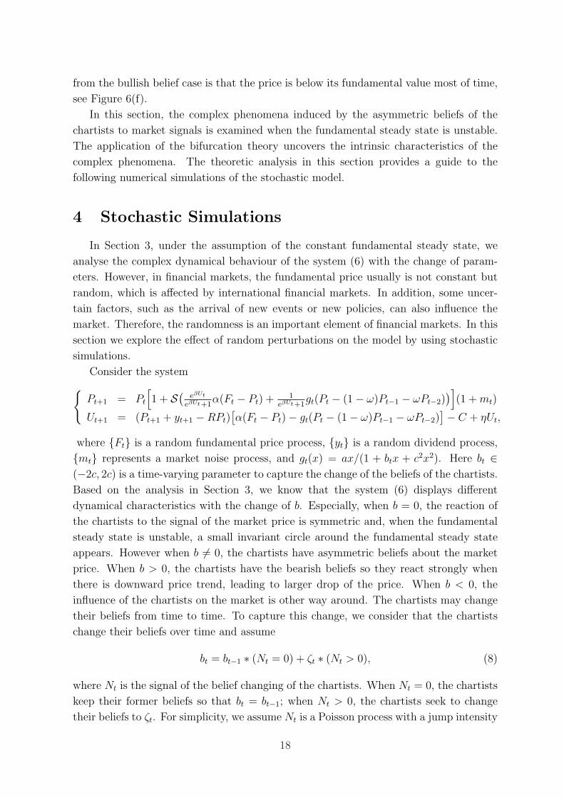
(a) (b)

Figure 4: The stable region of the steady state (P ∗2 , U∗

2 ) in the parameter space of (a, α, ω)

(a) and Dω∗ is denoted as the projection of D onto the plane ω = ω∗ (b).

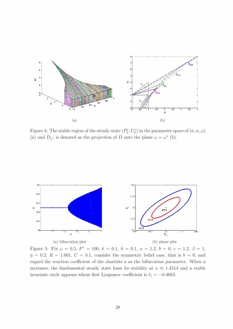
(a) bifurcation plot (b) phase plot

Figure 5: Fix ω = 0.5, F ∗ = 100, k = 0.1, h = 0.1, α = 1.2, b = 0, c = 1.2, β = 1,

η = 0.2, R = 1.001, C = 0.1, consider the symmetric belief case, that is b = 0, and

regard the reaction coefficient of the chartists a as the bifurcation parameter. When a

increases, the fundamental steady state loses its stability at a ≈ 1.4514 and a stable

invariant circle appears whose first Lyapunov coefficient is `1 = −0.4683.

28

(a) b < 0, a = 1.42 (b) b > 0, a = 1.42

(c) b < 0, a = 1.451 (d) b > 0, a = 1.451

(e) b < 0, a = 1.451, Time Series (f) b > 0, a = 1.451, Time Series

(g) b < 0, a = 1.46 (h) b > 0, a = 1.46

Figure 6: Fix ω = 0.5, F ∗ = 100, k = 0.1, h = 0.1, α = 1.2, c = 1.2, β = 1,

η = 0.2, R = 1.001, C = 0.1 and regard the reaction coefficient of the chartists a as the

bifurcation parameter. When b = −1.6 < 0 (left panel) and b = 1.6 > 0 (right panel), at

a ≈ 1.4514, the subcritical bifurcations occur and the stable fundamental steady state

with a stable invariant circle coexists (c), (d).

29

0 10 20 30 40 5099.6

100

100.4

100.8

t

P

0 10 20 30 40 50−1

0

1

t

0 10 20 30 40 500.41

0.44

0.47

0.5

0.53

t

n f

Df

Dc

+40000

+40000

+40000

(a) b < 0, a = 1.451

0 10 20 30 40 5099.4

99.7

100

100.3

t

P

0 10 20 30 40 50

−0.5

0

0.5

t

0 10 20 30 40 500.44

0.47

0.5

t

n f

Df

+40000

+40000

+40000

Dc

(b) b > 0, a = 1.451

Figure 7: When the coexistence of two attractors appears, the process of the price, excess

demands of the fundamentalists and chartists and market fractions corresponding to the

stable invariant circle are shown.

30

0 1000 2000 3000 4000 5000 600020

40

60

80

100

120

140

160

180

200

t

PF

(a) Risky asset price and its fundamental price

0 1000 2000 3000 4000 5000 6000−2

−1.5

−1

−0.5

0

0.5

1

1.5

2

b

t

(b) B-coefficient

0 1000 2000 3000 4000 5000 6000

−0.15

−0.1

−0.05

0

0.05

0.1

0.15

t

r

(c) Return of the risky asset price (r)

−0.1 −0.05 0 0.05 0.1 0.150

5

10

15

20

25

r

ReturnNormal

(d) Density of the return

−4 −3 −2 −1 0 1 2 3 4−0.2

−0.15

−0.1

−0.05

0

0.05

0.1

0.15

Standard Normal Quantiles

Quan

tiles o

f Retu

rn

(e) QQ-plot of the return

0 25 50 75 100 125 150

−0.05

0

0.05

0.1

0.15

0.2

lag

ACF(r)

(f) Autocorrelation of the return ACF (r)

0 25 50 75 100 125 1500.02

0.05

0.08

0.11

0.14

0.17

0.2

0.23

0.26

lag

ACF(|r|)

(g) Autocorrelation of the absolute return ACF (|r|)

0 25 50 75 100 125 1500

0.04

0.08

0.12

0.16

0.2

0.24

lag

ACF(r2)

(h) Autocorrelation of the squared return ACF (r2)

Figure 8: Simulation results.

31

2000 2100 2200 2300 2400 2500 2600 2700 2800 2900 300040

60

80

100

120

140

160

180

t

PF

(a) Risky asset price and its fundamental price

2000 2100 2200 2300 2400 2500 2600 2700 2800 2900 3000−2

−1.5

−1

−0.5

0

0.5

1

1.5

2

b

t

(b) B-coefficient

Figure 9: Enlargement of Figures 8(a), (b).

2300 2310 2320 2330 2340 2350 2360 2370 2380 2390 2400−0.2

0

0.2

0.4

0.6

0.8

1

1.2

t

nf

n

f

60

70

80

90

100

110

120

130

P

P

(a) Market fraction of the fundamentalists nf

and the risky asset price P

2300 2310 2320 2330 2340 2350 2360 2370 2380 2390 2400−0.2

0

0.2

0.4

0.6

0.8

1

1.2

t

nf

n

f

−100

−50

0

50

100

150

200

250

U

U

(b) Market fraction of the fundamentalists nf

and performance measure difference U = Uf − Uc

Figure 10: Herd behaviour

2000 2500 3000 35000.6

0.8

1

1.2

1.4

1.6

1.8

2x 10

4

t

AUf

AU

f

250

300

350

400

450

500

550

600

AUc

AU

c

Figure 11: Accumulative performance measure of the fundamentalists AUf and chartists

AUc, where AUq,t = AUq,t−1 + (Pt + yt −RPt−1)Dqt−1 − Cq (q = f, c).

32