Asymptotic Perron Method for Stochastic Gamesand Control

Mihai Sırbu, The University of Texas at Austin

Methods of Mathematical Financea conference in honor of Steve Shreve’s 65th birthdayCarnegie Mellon University, Pittsburgh, June 1-5, 2015

The important things first

Happy Birthday Steve!

Outline

Perron’s method

Previous workOne-player (control problems) and HJB’sGames and Isaacs equations

Perron’s method over asymptotic solutionsOne-player (control problems) and HJB’sGames and Isaacs equations: some modeling and results

Conclusions

Perron’s method

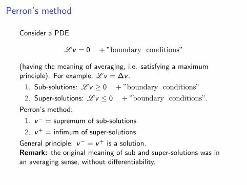
Consider a PDE

L v = 0 + ”boundary conditions”

(having the meaning of averaging, i.e. satisfying a maximumprinciple). For example, L v = ∆v .

1. Sub-solutions: L v ≥ 0 + ”boundary conditions”

2. Super-solutions: L v ≤ 0 + ”boundary conditions”.

Perron’s method:

1. v− = supremum of sub-solutions

2. v+ = infimum of super-solutions

General principle: v− = v+ is a solution.Remark: the original meaning of sub and super-solutions was inan averaging sense, without differentiability.

Perron and viscosity solutions

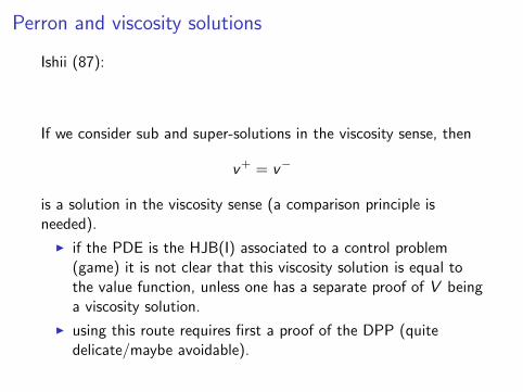
Ishii (87):

If we consider sub and super-solutions in the viscosity sense, then

v+ = v−

is a solution in the viscosity sense (a comparison principle isneeded).

I if the PDE is the HJB(I) associated to a control problem(game) it is not clear that this viscosity solution is equal tothe value function, unless one has a separate proof of V beinga viscosity solution.

I using this route requires first a proof of the DPP (quitedelicate/maybe avoidable).

Some previous modification of Perron for HJB’s

(joint with E. Bayraktar, SICON 13).

The Control Problem (without technical conditions):1. The state equation

dXt = b(t,Xt , ut)dt + σ(t,Xt , ut)dWt ,Xs = x ∈ Rd ,

starting at initial time s at position x , and which is controlled byone player u ∈ U. The BM W is d ′-dimensional.

2. A reward: g(X s,x ;uT ) at time T , g : Rd → R.

3. The value function

V (t, x) , supu

E[g(X s,x ;uT )].

The HJB and Stochastic semi-solutionsFormal HJB (for the value function)

Vt + supu Lut V = 0

V (T , x) = g(x)

where Lut V = b(t, x , u)Vx + 1

2Tr(σ(t, x , u)σT (t, x , u)Vxx).Idea: Use semi-solutions in the stochastic sense ofStroock-Varadhan (adapted to the non-linear case).

Definition (Stochastic semi-solutions)

1. w : [0,T ]× Rd → R is a super-solution if, for each s, x andeach control u the process (w(t,X s,x ;u

t ))s≤t≤T , is asuper-martingale and w(T , ·) ≥ g .

2. w : [0,T ]× Rd → R is a sub-solution if, for each s, x thereexist a control u such that the process (w(t,X s,x ;u

t ))s≤t≤T isa sub-martingale and w(T , ·) ≤ g .

Denote by U ,L the collections of super and sub-solutions in thestochastic sense as above.

Perron’s method over stochastic solutionsRemark: by construction we have

1. if w ∈ U then w ≥ V2. if w ∈ L then w ≤ V

Perron’s method:

1. v+ , infw∈U w ≥ V ,2. v− , supw∈L w ≤ V ,

sov− ≤ V ≤ v+.

Theorem (Bayraktar, S.)

Under some technical conditions, v+ is a USC viscositysub-solution and v− is a LSC viscosity super-solution.

Corollary

A comparison result for semi-continuous viscosity solutions implies

1. V the unique continuous viscosity solution of the HJB

2. the (DPP) holds, i.e. V (s, x) = supuE[V (τ,X s,x ;uτ )]

for all stopping times τ ≥ s.

Some previous work on games

(S. SICON 14):

I model symmetric games over feedback strategies, butrebalanced at discrete stopping rules (elementary feedbackstrategies for both players)

I use a Perron construction over sub/super-martingales to treatthe case of zero-sum symmetric games (where DPP is knownto be particularty delicate)

I the definition of stochastic semi-solutions has to be changedin a non-trivial way to account for the (dynamic) strategicbehavior

I upper and lower value functions are solutions of the Isaacsequations

I (versions) of the (DPP) for games are obtained

More about games to follow.

Some comments (on previous work)

I the proofs are rather elementary. The analytical part mimicsthe proof of Ishii and then we apply Ito to the (smooth) testfunctions.

I amounts to verification for non smooth solutions

I proving a DPP is particularly complicated for games(Fleming-Souganidis)

Perron’s method over asymptotic semi-solutions

Goal: design a modification of Perron’s method that works wellwith discretized Markov controls/strategies (in a similar elementaryway).

Simple Markov strategies (in one player problems)Fix 0 ≤ s ≤ T . A path of the state equation is a y ∈ C [s,T ].

Definition (time grids, simple Markov strategies)

1. A time grid for [s,T ] is a finite sequence π ofs = t0 < t1 < · · · < tn = T .

2. Fix a time grid π as above. A feedback strategy

α : [s,T ]× C [s,T ]→ U,

is called simple Markov over π if there exist some measurablefunctions αk : Rd → U, k = 1, . . . , n such that

α(t, y(·)) =n∑

k=1

1tk−1<t≤tkαk(y(tk−1)).

I A M(s, π): simple Markov strategies over π

I A M(s) ,⋃π A M(s, π) all simple Markov strategies

Use only simple Markov strategiesDefine

Vπ(s, x) , supα∈A M(s,π)

E[g(X s,x ;α,vT )] ≤ V (s, x).

and the value function over all simple Markov strategies

VM(s, x) , supα∈A M(s)E[g(X s,x ;αT )] = supπVπ(s, x) ≤ V (s, x).

Natural question: can the value function be approximated bydiscretized Markov strategies, i.e. VM = V ?

Under some technical conditions, Krylov has proved this propertyusing PDE arguments and regularity properties of the valuefunction (obtaining the DPP also).Some Perron-type construction may be simpler (work for games?)

I the previous method cannot show that. Why? Because, ifw ∈ L then we do not know that w ≤ V M

I if we use simple Markov strategies in the Def of L the PerronConstruction does not work anymore.

Need for new concept of sub-solution of the HJBModify the definition of sub-solutions (only) such that

1. sub-solutions w stay below VM

2. w− , sup w ≤ VM is still a viscosity super-solution

Intuition: consider a (strict) smooth sub-solution of the HJBwt + supu Lu

t w > 0V (T , x) ≤ g(x).

Start at time s at position x with the feedback control attainingthe sup above (argmax u∗ = u∗(s, x)) and hold it constant untilT . The process

(w(t,X s,x ;u∗

t ))s ≤ t ≤ T

is a sub-martingale until the first time τ when wt + Lu∗t w ≤ 0.

However,P(τ ≤ t) = o(t − s).

In between s and t we have a sub-martingale property plus ano(t − s) correction.

Asymptotic sub-solutions, precise definition

Take the previous observation and make it (more) dynamic.

Definition (Asymptotic Stochastic Sub-Solutions)

w : [0,T ]× Rd → R is called an asymptotic sub-solution if it is(bounded), continuous and satisfies w(T , ·) ≤ g(·).There exists a gauge function ϕ = ϕw : (0,∞)→ (0,∞),depending on w such that

1. limε0 ϕ(ε) = 0,

2. for each s, and for each time s ≤ r ≤ T , there exists ameasurable function α : Rd → U such that, for each ξ ∈ Fr ,if we start at the time r at the (random) condition ξ and keepthe feedback control α(ξ) constant on [r ,T ] we have

w(r , ξ) ≤ E[w(t,Xs,ξ;α(ξ)t )|Fr ] + (t − r)ϕ(t − r) a.s.

Denote by La the set of asymptotic sub-solutions.

Important property of asymptotic sub-solutions

LemmaAny w ∈ La satisfies w ≤ VM ≤ V .

Proof:

1. Fix ε, then fix δ such that ϕ(δ) ≤ ε. Choose ‖π‖ ≤ δ2. construct, recursively, going from time tk−1 to time tk , some

measurable αk : Rd → U satisfying the Definition 5.

3. for α(t, y(·)) =∑n

k=1 1tk−1<t≤tkαk(y(tk−1)) we have

w(tk−1,Xs,x ;αtk−1

) ≤ E[w(tk ,Xs,x ;αtk )|Ftk−1

] + ε(tk − tk−1)

Telescoping sum: w(s, x) ≤ E[w(T ,X s,x ;αT )] + ε(T − s).

Summary: if |π| ≤ δ(ε) there exists α ∈ A M(s, π) such that

w(s, x) ≤ E[g(X s,x ;αT )] + ε× (T − s) ≤ Vπ(s, x) + ε(T − s).

Letting ε 0 we obtain the conclusion.

Perron method over asymptotic sub-solutionsDefine

w− , supw∈La

w ≤ VM ≤ V .

Theorem (Perron over asymptotic sub-solutions, HJB)

The function w− is an LSC viscosity super-solution of the HJB.

I the proof is (again) based on the analytic construction of Ishii

I negating the viscosity super-solution property, the testfunction is a strict classic sub-solution (locally)

I apply Ito to the test function, together with a very similarobservation we made for strict classic sub-solution, i.e.sub-martingale property plus an o(t − r) correction.

Corollary

A comparison result (which holds under some technicalassumptions) implies that VM = V and, actually, Vπ V as‖π‖ 0 uniformly on compacts.

Overview of the method

I adding a correction to the sub-martingale property (overfeedback controls), we have a (rather elementary) tool toapproach Dynamic Programing over simple Markov strategiesfor control problems.

I we can apply it to games, where the Dynamic Programmingarguments are more difficult

Zero-sum differential games

1. The state equationdXt = b(t,Xt , ut , vt)dt + σ(t,Xt , ut , vt)dWt ,Xs = x ∈ Rd ,

starting at initial time s at position x , and which is controlled byboth players.

2. A penalty/reward: (if a genuine game) the second player (v)pays to the first player (u) the amount g(X s,x ;u,v

T ) at time T .

Formal zero-sum game

supu

infvE[g(X s,x ;u,v

T )], infv

supu

E[g(X s,x ;u,vT )].

Inputs of the game

I the coefficients of the state equation b, σ

I the sets where the two players can take action: u ∈ U, v ∈ V

I for each initial time s, a (fixed) probability space (Ω,F ,P)and a Brownian motion W with respect to the filtration(F s

t )s≤s≤T . Allow the filtration to be larger than the onesgenerated by W .

Standing assumptions

I g is continuous and bounded,

I b and σ are continuous on their whole corresponding domainsand (locally) uniformly Lipschitz in x and have linear growth.

I U,V are compact

ObjectiveLook at

I modeling of such gamesI apply the Asymptotic Perron tool to the dynamic

programming analysis:I relate the value functions to Dynamic Programming

Equation(s)I (more important) study existence of value for the game:

sup inf = inf sup

Why?

I Unlike one player (control) problem, it is unclear what to usefor u, v . There is no widely accepted notion ofstrategy/control, so no ”canonical” formulation anyway(Cardaliaguet lecture notes).

I the dynamic programming analysis (i.e. relation to Isaacsequation) is significantly more complicated (seeFleming-Souganidis, for an Elliott-Kalton formulation of thegame)

Some literature on games

Very selective list of works

I Isaacs: deterministic case over (heuristically) feedbackstrategies

I Krasovskii-Subbotin: engineering-type literature, veryinteresting modeling over feedback strategies andcounter-strategies

I Elliott-Kalton: deterministic case, use so called strategies forthe stronger player, (open loop) controls for weaker player (nosymmetric formulation)

I Fleming-Souganidis: use Elliott-Kalton strategies in stochasticgames. Prove the value functions are viscosity solutions ofDPE (Bellman-Isaacs equations). No symmetric formulation.

I large interesting literature on games studied using BSDE’s:Hamadene and Lepeltier, El Karoui-Hamadene, Buckdahn-Li(more others)

Literature cont’d

1. Most of the mathematical literature uses an Elliott-Kaltonformulation. Value functions do not compare by definition, butafter complicated analysis. Actually, the value functions belong todifferent games, depending on one player or another having aninformational advantage.

2. Ekaterinburg school of games (mainly Krasovskii-Subbotin): use(discretized) feedback strategies (mostly in) deterministic games.Recently, symmetric formulation of games where both players usestrategies based only on the knowledge of the past of the statehave been re-considered:

I Cardaliaguet-Rainer ’08 (strong formulation, path-wisefeedback strategies with delay)

I Pham -Zhang ’12 (path-wise feedback strategies, discretizedin time and space, called ”feedback controls”)

The model(s) we use for games

We continue the line of modeling with feedback strategies andcounter-strategies in Krasovskii-Subbotin and recently inFleming-Hernandez-Hernandez.

The lower Isaacs equation

Formal equation: Vt + supu infv Lu,v

t V = 0V (T , x) = g(x)

whereLu,vt V = b(t, x ; u, v)Vx + 1

2Tr(σ(t, x ; u, v)σT (t, x ; u, v)Vxx).

I analytic representation of a game where v has aninformational advantage over u

I would like to model this situation using feedback strategies

Feedback strategies

(Krasovskii-Subbotin, Cardaliaguet-Rainer, Pham-Zhang)The player using such strategy

I observes the state only

I does not observe the other player’s actions

I do not observe the noise

Therefore, if C ([s,T ]) is the path-space for the state, we canconsider

α : (s,T ]× C [s,T ]→ U

ORβ : (s,T ]× C [s,T ]→ V

adapted to the filtration B = (Bt)s≤t≤T defined by

Bst , σ(y(u), s ≤ u ≤ t), 0 ≤ t ≤ T .

As for one player, we denote by y the paths of the state equation.

Feedback counter-strategies for v

(following Krasovskii-Subbotin)

I player u can only see the state

I the player v observes the state, and, in addition, the control u(in real time)

Intuition: the advantage of the player v actually comes only fromthe local observation of ut . A counter-strategy for v depends on

1. the whole past of the state process X up to the present time t

2. (only) the current value of the adverse control ut .

Definition (Feedback Counter-Strategies)

Fix a time s. A feedback counter-strategy for the player v is amapping

γ : [s,T ]× C [s,T ]× U → V ,

which is measurable with respect to Ps ⊗U b/V . The action ofthe player v is vt = γ(t,X·, ut).

More ways to think about the game

where v has an advantage over player u:

1. the lower value of a symmetric game over feedback strategiesi.e. u announces the strategy to v (Pham-Zhang, S.)

2. the value function of a robust control problem where u is anintelligent maximizer (using feedback strategies) and v is apossible worst case scenario modeling Knigthian uncertainty(see S.), or

3. the genuine value of a sup-inf/inf-sup non symmetric gameover feedback strategies vs. feedback counter-strategies(Krasovskii-Subbotin, Fleming -Hernandez -Hernandez).

Strategies/counter-strategies and open-loop controls

Well-posedness of the state eq with feedback strategies orcounter-strategies is important, but we disregard it here.

Denote by U (s) and V (s) the set of open-loop controls for theu-player and the v -player, respectively. Precisely,

V (s) , v : [s,T ]×Ω→ V | predictable w.r.t Fs = (F st )s≤t≤T,

and a similar definition is made for U (s).

Notation/symbols

1. α, β for the feedback strategies of players u and v ,

2. u, v for the open loop controls,

3. γ for the feedback counter-strategy of the second player v .

Value functions1. lower value function for the symmetric game in between twofeedback players:

V−(s, x) , supα∈A (s)

(inf

β∈B(s)E[g(X s,x ;α,β

T )]

).

2. the value of a robust control problem where the intelligentplayer u uses feedback strategies and the open-loop controls vparametrize worst case scenarios/Knightian uncertainty:

V−rob(s, x) , supα∈A (s)

(inf

v∈V (s)E[g(X s,x ;α,v

T )]

).

3. Lower and upper values of a non-symmetric game overstrategies α vs counter-strategies γ

W−(s, x) , supα∈A (s)

(inf

γ∈C (s)E[g(X s,x ;α,γ

T )]

)≤

infγ∈C (s)

(sup

α∈A (s)E[g(X s,x ;α,γ

T )]

), W +(s, x).

Value functions cont’d

For mathematical reasons, we define yet another value function

V +rob(s, x) , inf

γ∈C (s)

(sup

u∈U (s)E[g(X s,x ;u,γ

T )]

)≥W +(s, x). (1)

We attach to V +rob the meaning of some robust optimization

problem, but this is not natural, since the intelligent optimizer vcan see in real time the “worst case scenario”.

By simple observation

V−rob ≤W− = V− ≤W + ≤ V +rob.

Simple Markov strategies/counter-strategies definition

Recall we have defined Markov strategies already for one-player.

Definition (simple counter-strategies)

Fix 0 ≤ s ≤ T . Fix a time grid π as above.A counter-strategy γ ∈ C (s) is called a simple Markovcounter-strategy over π if there exist some functionsηk : Rd × U → V , k = 1, . . . , n measurable, such that

γ(t, y(·), u) =n∑

k=1

1tk−1<t≤tkηk(y(tk−1), u).

Notation:

I CM(s, π) is set of simple Markov counter strategies over π

I CM(s) ,⋃π CM(s, π) is the set of all simple Markov

counter-strategies.

State equation and value functions with Markov strategies

The state equation is well posed if one player is using simpleMarkov strategies or counter-strategies and the opposing player isusing open-loop controls.

If we use Markov strategies or counter-strategies in the LHS, RHSthey are well defined.

V−M (s, x) , supα∈A M(s)

(inf

v∈V (s)E[g(X s,x ;α,v

T )]

)≤ V−rob(s, x)

as well as

V +M (s, x) , inf

γ∈CM(s)

(sup

u∈U (s)E[g(X s,x ;u,γ

T )]

)≥ V +

rob(s, x).

Main result/games

Theorem (S.)

Under the standing assumptions

I all value functions are equal: V−M = V +M = the uviscosity

solution of the lower Isaacs equation.

I the game α vs γ has ε-saddle points over simple Markov α’sand γ’s.

(More) precisely: ∀ N, ε > 0, ∃ δ(N, ε) > 0 such that∀s,∀ |π| ≤ δ, ∃ α ∈ A M(s, π), γ ∈ CM(s, π) for which

0 ≤W−(s, x)− infv∈V (s)

E[g(X s,x ;α,vT )] ≤ ε

and0 ≤ sup

u∈U (s)E[g(X s,x ;u,γ

T )]−W +(s, x) ≤ ε.

Conclusions

I dynamic programming arguments (the proof of the DPP) areclean only for discrete-time problems (Blackwell, Berstekasand Shreve)

I the (direct) proof of the DPP is more delicate forcontinuous-time problems

I Perron’s method and its modifications appear to be useful inthe dynamic programming analysis of continuous-timeoptimization problems, allowing for a verification withoutsmoothness

I the asymptotic modification of Perron (adding a correction tomartingales) is the last step in the program. It provides thestrongest conclusion expected in a non-smooth case: cannotget more without smoothness of the solutions of the HJB(I)

I the case of games is of particular interest, since usual dynamicprogramming arguments run into even more difficulties there(Fleming-Souganidis)

For gamesThere are three possible interpretations of the game that lead tothe lower Isaacs equation

1. lower value of a a symmetric over (restricted) feed-backstrategies

2. a control problem of model uncertainty3. the true value of a game over strategies vs. counter-strategies

Using Perron method over asymptotic solutions, we connect (in aunified way) all three problems.More important: find an (approximate) saddle point over Markovstrategies and counter-strategies.Remarks:

I it is important how we define both the game and thesemi-solutions (asymptotic correction)

I we have flexibility in defining semi-solutions (to make theproofs work, but keep comparison with the value functionobvious)

I filtrations do not matter (just as if solutions to the Isaacsequation were smooth).