ASYMPTOTIC PROPERTIES OF A STOCHASTIC EM

ALGORITHM FOR ESTIMATING MIXING PROPORTIONS

by

Jean DieboltGillesCeleux

TECHNICAL REPORT No. 228

October 1991

Department of Statistics, GN-22

University of Washington

Seattle, Washington 9819S USA

Asymptotic Properties of a Stochastic EMAlgorithm for ·Estimating Mixing

Proportions

LSTA, Paris Cedex 05

INRIA

Abstract

Chesnay Cedex

The purpose of this paper is to study the asymptotic behavior' of the Stochasticin a simple case within the mixture context.

of Washing;ton, ::iea1ttle;oont,ract N-OOOl4-91-J-I074.

1

1 Introduction

of these drawbacks, wealgorit~rn, •. lhat we

'-''-'~',",U'" and Diebolt (1983)Instes,d of maximizing the eXT>ected cmnplet!e­

lO~~ll1<~ell.OOd conditional on the observations X(N) =algorithm first simulates the missing data Z(N) from the conditional

density k(Z(N)lx(N),o(m)), where o(m) is the current guess of the parame­ter, and then computes the maximum of the pseudo-completed likelihoodfunction, thus producing the updated estimator o(m+l). Note that the SEMalgorithm can be seen as a particular case of the MCEM algorithm of Weiand Tanner (1990), with q = 1 in their notation, and that these authors

nnrn,,,,,,,,, of is to study the as\rmlptc,tlC '-J"-"U,LV'Vl.

rall(l(:>m sequence of parameters generated by the Stochastic EM alJ!:onthlffi(j,lgorrthIlI1, see, Celeux and Diebolt (1985)) as the sample

a simple particular case within the mixture context.EM algorithm (Dempter, Laird and Rubin, 1977) is a widely appli­

apprc>ach for computing maximum likehood (ML) estimates for incom­.LJ'-"JIJ~"'-' appealing features, the EM algorithm has several severe

cmnpofiient;s IS sutllclent to ensure conver-

2

the distributions considerationveau (1991) makes use of SEM for this reason when dealing with mixturesof \Veibull distributions.

The numerical simulation results of Celeux and Diebolt show that thestationary distributions \IfN of SEM is usually concentrated around a signif­icant local maximum of the likelihood. In the present paper, we address thefollowing basic problems :

1

2. What is the order of (Jj:Jm (IN, where (IN is the unique consistentsolution of likelihood equations Redner Walker, 1984) ?

IS concave

3

COl1rS,e, in a case, EM gives good and fromview, SEM is not useful. However, results obtained in

partH:::Ul,ar case have own theoretical and permit uswhat is really and the mathematics beyond Problems

J.C;;:'UJ.l," suggest what answers can be expected inmore general situations.

In Section 2, we present the simple mixture model that we will considerthroughout the paper and derive preliminary results about the l.f., EM andSEM in this particular case.

Section 3 is devoted to our main result, stated as Theorem 1. This the­atJJlrrrlatlve answers to Problems (1) and (3) for the model un-

also a (non-optimal) estimate of the rate ofas an estimate of the rate of the conditional

variance X(lV)' Furthermore, the results in Theorem 1 implythat 0Nm is an asymptotically unbiased and optimal estimator of () and thestationary rescaled SEM sequence y(m) N 1/ 2 ( ()(m) ON) converges in dis­tribution, as N -+ 00, to the distribution of the stationary autoregressivesequence {Zim

)} defined by

z(m+l) = r* z(m) +O"*E(m)* * , (1.1 )

nTh",,.,,, the E(m)'S are Gaussian i.i.d. random variables with mean 0 and vari­is depegdentofZio), ... , Zim),iand ,0 < r* < 1, and 0"*.'0"* > 0,

del1n€:d in (2.8) and (2.19) in terms of the complete, conditional and ob­served Fisher information values, respectively.

~e(;tlO>fi 4 two different sequential versions of SEM. The "one-vel:sic,n has implicitly studied in Silverman (1980), but <has its

as-yrmlDtc~tlcefficiencycanequal to zero. Our Theorem 3 states the a.s. conver­as-yrmlDto,tic normality. Since

eXIDIH31t, we can examine in detail its as:\,m1ptc,ticetJJlcl~mc:y. which turns out to be of the same order as the optimal bound.

4

2 Preliminary results

2.1 The mixture problem

Throughout this paper, the observed data X(N) = {Xll' .. , XN} willizations of i.i.d. random variables from the mixture density h(x,p*), where

h(x,p) = ph(x) +(1 - p)fz(x), (2.1)

where fl(X) and Jz(x) are known densities with respect to a a-finite measurep,(dx) on some separable measurable space E, and parameter p satisfieso< p < 1. We will : h(x);:j:. ;:j:. 0. and that fl(X)and Jz (x) are positive The statistical problemunder consideration is to a good of p* the basis of X(N).

Before proceeding, a formal point to be made, <since the study of theasymptotic behavior as the sample size N -+ 00 of a stocha:;;;tic algorithminvolves two different probability spaces: The sample space and the sampleof pseudorandom drawings. We will interpret each sample X(N) of size Nas the projection on the N first coordinates of a sequence x = {Xi; i ~ I}drawn from the product space X = E{i:i~l} endowed with the probabilitydistribution

00

Px = II h(Xi,p*)dxi'i=l

(2.2)

The formal description of the pseudorandorn drawings is postponed Sub-section 2.3.

Next, let us describe the underlying complete data structure of the sta­tistical problem under consideration. The complete data is (x(N), Z(N») ={(Xi,Zi);i = 1, ... ,N}, where Zi lor oaccording as Xi has been drawnfrom fl(X) or Jz(x), and the are independent. Thus, each a Bernoullir.v. with parameter p*), nTh",,,.:>

(2.3)

2.2 The EM algorithm

5

p) PE(0,1). (2.4)

o - indeed consistsfunction TN : [0,1] ~ [0,1], starting from an initial position

We have the following preliminary results, where

N

L log h(xi, p)i=l

(2..5)

nhl,prlllPr! cornpJete andconditionalare defined as

Lemma 2.1 (i) The function TN(p) is increasing over [0,1].

(ii) vVe have, for all P in [0,1],

TN(p) - P p(1 _ p) L:~p). (2.6)

(iii) For Px-almost every x E X, there exists an integer No = No(x) such'Wnl~ne'Vt:1" N ~ N OI i. the loglikeli-

(iv) IfpN is the unique maximizer of LN(p) when N ~ NOI PN is the uniquestable fixed point over [0,1], with

(2.7)I .......;:.;--:.-.-:... E (0, 1),

(v) starting from p(Oj E (0,1) con-

aerzvaltzve TN of at c011~ve1'(Jes PX-a.s. to

1- E

as ~ 00.

6

(2.9)

A brief proof of Lemma 2.1 can be found in the AppelldlX.

Remark 2.1 - Lemma 2.1 shows that, in the simple incomplete data statis­tical problem under consideration, ElY does very well if N ~ . Thus, froma practical point of view, the're is no need for any improved algorithm in thisparticular case. However, we have explained in Section 1 why the asymptoticbehavior of SE1Y as N -7 00 in this context deserves a ca'reful study.

2.3 The SEM algorithm

In the present context, the Stochastic Imputation Principle (e.g., Celeuxand Diebolt, 1987) produces the updated estimate p(mH) as theMLesti-mate based on the pseudo-completed sample (X(N)J z(m») = {(Xi, z!m»); i ­

1, ... ,N}, where z(m) E Z(N) = {O, 1}N, each z!m) is a Bernoulli r.v. with

parameter t~m) = t(Xi, p(m») given by (2.3) and the z!m),s, i = 1, ... ,N, aredrawn independently. This yields, in view of (2.4),

(m+l) _ 1 ~ (m)p - N ~Zi ,

t=l

so that the random sequence {p(m)} is a homogeneous Markov chaintakillg itsvalues in {O, ~, ... , N;/, 1}. In order to remove the absorbing states oandI ,we first make choice of a sequence of thresholds c(N), .~ ::; c(N) < 1-c(N) ::;

, such that c(N) -7 0 as N -7 00, and of a probability distribution r N

on the set {# : j = 0,1", . ,N and c(N)::; ::; 1 - c(N)}. The SEM

algorithm then proceeds as follows. E-step: Compute p(m») t}m) fori = 1" .. ,N using (2.3). S-step: For i - ... ,N, independently theBernoulli r.v.'s z!m) with parametert}m) and compute

(m+!) 1 ~p 2 =-L..,;

i=l

(2.10)

7

11

p = °or p = 1, wh,ere.OtS

Lemma 2.2 The } by SEM isgeometrically ergodic and the support of its stationary distribution \fiNiscontained in JN.

The proof of Lemma 2.2 can found the Appelld1X.

Remark 2.2 - As a consequence, since {p(m)} is a ergodic Markovchain, it is uniformly strongly mixing with a geometric rate. Hence, the SLLNand a suitable version of the CLT (e.g., Davydov, 1973) apply.

vVe conclude this section by showing that the sequence generated by SEMcan be viewed as a random perturbation of the discrete-time dynamical sys­tem on [0,1] generated by EM. First, we need to have a workable represen­tation of the r.v.'s z}m). They can be written as

(m)z·t 1 ( (m») . - 1 1\T

[O,t(Xi,p(m)j Wi ,~-, •.• , 1 ~, (2.12)

where 1[a,bj (s) is the indicator function of the interval [a, b] and the Wi'S,

i 1, ... , N, are i.i.d. random variables uniformly distribued on [0,1] suchthat the sample w(m) = (wim), ... ,w~») is independent of p(O), ... ,p(m). Wehave

p(m+~) = TN(p(m») +UN(p(m»),

nth",,.,,, for each p, °< p < 1,

UN(p) = N-1/2SN(p)rnv(p,w),

urh"'''''' SN(P) > 0, SJv(p) = p(1 p)TJ..r(p) con'ver.e:es "'''''->1 '"

(2.13)

(2.14)

as N ----t 00 to

(2.15)

r.v. w ----t

i:::1

mean 0 and variance 1 each pin (0,1). \Vith representation's, the probabilistic setup of the successive random drawings in­

the S-step of SEM can be made precise: each w(m) can be viewed asa sequence of n = [0,1 j{i:i;:::l} endowed with the product o--field and thepr()ba,bllltv Po(dw) = ni>lA(dwi ), where A denotes the Lebesgue measure on[0, ll, whereas 'f/N(p, w(m») only involves the first N coordinates wim), ... ,w~m)of the sequence w(m). We will denote by Eo(Y) the expectation of any r.v.Y(w) with respect to this probability Po. For instance, EO('!JN(p,W)) = 0and Eo{'!J~(p,w)}= 1 for all pin (0,1).

Since the CLT implies that, for all pin (0,1) and Px-a.e. x, '!IN(p,W)converges in Po-distribution as N -+ 00 to a Gaussian r.v. c(w) with meanoand variance 1, we can expect that, for large N, (2.10)-(2.14) can be ap­proximated by

(2.17)

with c(m) = c(w(m»), so that, if we can show that the stationary measure\]!N of {p(m)} is well concentrated around PN, then (2.17) turns out to beapproximately

(2.18)

Furthermore, since r N -+ r* and

(2.19)

as 1'1 -+ 00,

(2.20)

so that, in general, p(m+1) = p(m+~) if p(m) remains near PN most of the time.If we can make the approximations (2.17)-(2.20) precise and uniform withrespect to p(m) a suitable sense and show that p(m) remains near PN, thenwe will proved Theorem 1, which we will now state and prove.

9

3 Main Results

3.1 Theorem 1

Before stating our Theorem 1, we to mtl~odluce

R(N) = R(x, N) = suppEJN,P:j:.PN

(3.1)

Appendix that 0 <-+ 0 as c(N) -+ O.

It follows from the results in Subsection 2.2 andR(N) < 1 Px a.s. for large 1Furthermore, the rate of COIweJrgeJtlceprovided that rate

Them'em 1 Suppose that the foli:ow'ina assumpU,rms(Hi) The densities 11(X) and JL{x:(H2) The probability distribution r N (see Subsection 2.3) used to draw theupdated SEM estimator p(m+l) when p(m+(1/2» is not in IN is the Dirac mea­sure at some j(N)/N E (c(N), 1 - c(N)), 1 S j(N) S N - 1.(H3) Nc(N) -+ 00 as N -+ 00.

(H4) N{l - R(N)}4 -+ 00 as N -+ 00.

Then

(i) IfWN isN 1/ 2(WN - a r.v.w·ith mean 0 and variance v* = (J"*2/ (1 - r*2), where 1'* = Jcond / Jc E(0,1) and (J"*2 = p*(l - p*)r* = Jcond/Jr

(ii) For all large enough,

=0 {--

and(3.5)

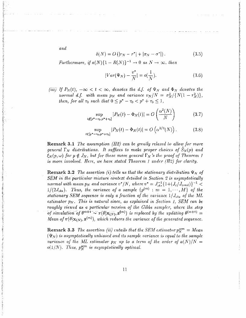
Furthermore, if a(N){1 R(N)} -1 -+ 0 as N -+ 00, then

IVar(WN)v* 1N l = o(N)' (3.6)

(iii) If PN(t), -00 < t < 00, denotes the d.j. of WNand <PN denotes thenormal d.j. with mean PN and variance vN/N = o-~/{N(1 r~)},

then, for all TO such that 0 :::; p* - TO < p* + TO :::; I,

sup IPN(t) - <PN(t)1 = 0 ((?/3(N)). (3.8)tE[P*-ro,p*+ro]

Remark 3.1 The assumption (H2) can be greatly relaxed to allow for moregeneral r N distributions. It suffices to make prope1' choices of SN(p) andeN(p,W) for P f:. IN' but for these more general Cv's the proof of Theorem 1is more involved. Here, we have stated Theorem 1 under (H2) for clarity.

Remark 3.2 The assertion (i}tells us that the stationary distribution WN ofSEM in the particular mixture context detailed in Section 2 is asymptoticallynormal with mean PN and variance v* / N, where v* = J;;b;{l+(Jc / Jcond )} -1 <1/(2Jobs)' Thus, the variance of a sample {p(m) : Tn = 1"", M} of thestationary SEM sequence is only a fraction of the variance 1/Jobs of the MLestimator PN. This is natural since, as explained in Section 1, SEM can beroughly viewed as a particular version of the Gibbs sampler, where the stepof simulationojOm+1 f"'-J 1r(Olx(N)I z(m») is replaced by the updating o(m+1) =NIean of1r(Olx(N), z(m»), which 1'educes the variance of the generated sequence.

Remark 3.3 assertion entails that the SENI estimator = l\feanasymptotically unbiased and its sample variance is equal to the sample

1lf1'Y'?f1'fL('P of to a of the of -zs as~,m~Jtoitic(~lly o~n;Zm(Zl.

11

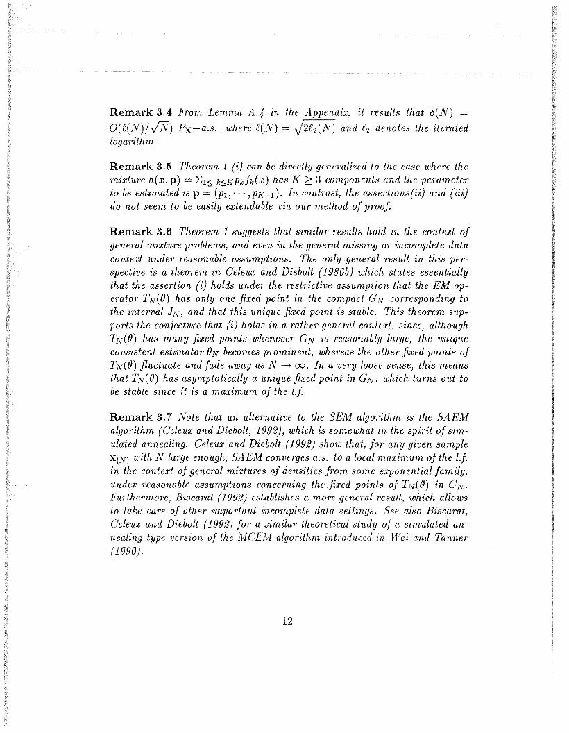
Remark 3.4 From Lemma A.4 m

O(f(N)jVN) Px-a.s., wherelogarithm.

results that o(N) =

aerWTA~S the iterated

Remark 3.5 Theorem 1 (i) can be directly generalized to the case where themixture h(x,p) = :El~ k~KPkfk(x) has I< 23 components and the parameterto be estimated is p = (Pl,'" ,PK-d. In contrast, the assertions(ii) and (iii)do not seem to be easily extendable via our method of proof.

Remark 3.6 Theorem 1 suggests that similar results hold in the context ofgeneral mixture problems, and even in the general missing or incomplete datacontext under reasonable assumptions. The only gene'ral result in this per­spective is a theorem in Celeux and Diebolt (1986b) which states essentiallythat the assertion (i) holds under' the restrictive assumption that the EM op­erator TN(O) has only one fixed point in the compact GN corresponding tothe interval JN, and that this unique fixed point is stable. This theorem sup­ports the conjecture that (i) holds in a rather general context, since, althoughTN(O) has many fixed points whenever GN is reasonably large, the uniqueconsistent estimator ON becomes prominent, whereas the other fixed points ofTN(O) fluctuate and fade away as N -+ 00. In a very loose sense, this meansthat TN ( 0) has asymptotically a unique fixed point in GN , which turns out tobe stable since it is a maximum of the l.f.

Remark 3.7 Note that an alternative to the SEjVf algorithm is the SAEMalgorithm (Celeux and Diebolt, 1992), which is somewhat in the spirit of sim­ulated annealing. Celeux and Diebolt (1992) show that, f01' any given sampleX(N) with N large enough, SAE..."AJ. converges a.s. to a local maximum of the 1.f.in the context of general mixtures of densities from some exponential family,under reasonable assumptions concerning the fixed points of TN(O) in GN.Furthermore, Biscarat (1992) establishes a more general result, which allowsto take care of other important incomplete data settings. See also Biscarat,Celeux and Diebolt (1992) for a similar theoretical study of a simulated an­nealing type version of the Il/lCEA! algorithm introduced Wei and Tanner(1990).

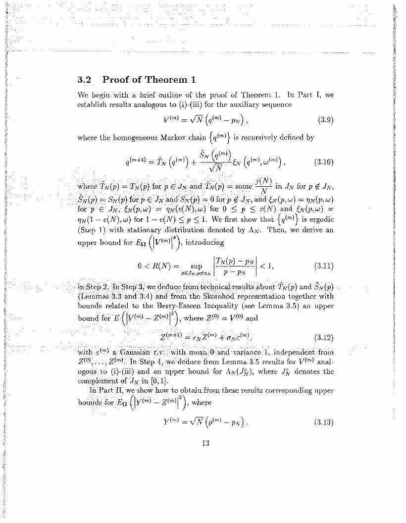
3.2 Proof of Theorem 1

a 1. Part I, we

(3.9)

where the homogeneous Markov chain {q(m)} is recursively defined by

(3.10)

(3.11)

IN for P t¢ IN'

w) t"fN(p,W)IN' w) for P ::; and eN(p,W) =

t"fN(l c(N), w) for 1 - c(N) ::; P ::; 1. We first show that {q(m)} is ergodic(Step 1) with stationary distribution denoted by AN. Then, we derive an

upper bound for Eo (Iv(mf), introducing

0< R(N) = sup ITN(p) - PN 1< 1,pEJN,P:f:PN I P - PN I

bounds related to the Berry-Esseen Inequality (see Lemma 3.5) an upper

Z(1n)f), = y(O) and

(3.12)

rp"111It" for y(m) anal­I N derLOtt~S

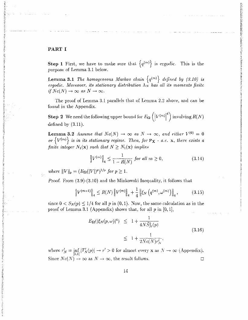
PART I

Step 1 First, we have to make sure that {q(m)} is ergodic. IS

purpose of Lemma 3.1 below.

Lemma 3.1 The homogeneous Markov chain {q(m)} defined by (3.10) isergodic. Moreover, its stationary distribution AN has all its moments finiteif N c(N) -+ 00 as N -+ 00.

The proof of Lemma 3.1 parallels that of Lemma 2.2 above, and can befound in the Appendix.

Step 2 We need the following upper bound for Eo (Iv(mf) involving R(N)

defined by (3.11).

Lemma 3.2 Assume that Nc(N) -+ 00 as N -+ 00, and either V(O) = 0or {v(m)} is in its stationary regime. Then, for Px - a. e. x, there exists a

finite integer N 1(x) such that N ~ N 1(x) implies

II v (m)114 ::; 1 ~(N) for all m ~ 0,

where IIVllp = (Eo(IVI)P)l/p for p ~ 1.

Proof. From (3.9)-(3.10) and the Minkowski Inequality, it follows that

(3.14)

(3.1.5)

since 0 < SN(p) ::; 1/4 for all p in (0,1). Now, the same calculation as in theproof of Lemma 3.1 (Appendix) shows that, for [0,1J,

(3.16)1

< 1 + --.....,--

-+ 1" > 0

-+ 00,

xas -+00

o

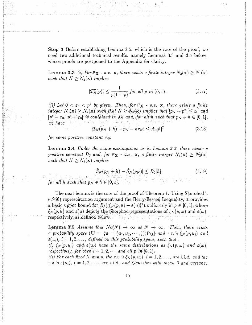
core proof, we3.4 below,

Step 3 tlelore est;:l,blllShlrlJ?; LeIIlIIla

two aGdlltlcmal tec.hmc.al reslilts, naIneJ.y Ll~mrnas

\,vhj()qp proofs are postponed to

Lemma 3.3 - a.e. x,such that N 2: N2(x) implies

ITN(p) I :::; (1 ) for all p in (0,1).p1-p

(3.17)

(ii) Letinteger

co,have

exists a finitecoo.nd

E [0,1],

(3.18)

for some positive constant Ao.

Lemma 3.4 Under the same assumptions as in Lemma 3.3, there exists apositive constant Eo and, for Px - a.e. x, a finite integer N4(x) 2: N3(x)such that N 2: N4 (x) implies

(3.19)

for

Then, there existsr.v. 's eN(p, Ui) and

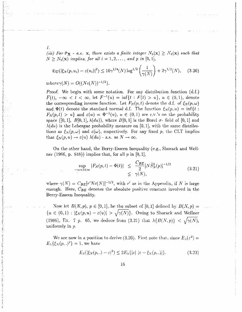
1.(iii) For Px - a.e. X, there exists a finite integer N5(x) ~ N4 (x) such thatN ~ for all i = 1,2, ... , and P [0,1],

Eu(leN(p, Ui) - e(ui)1 2) ~ 1O,1/4(N) logl/2 (,(~)) + 2,1/2(N), (3.20)

where,(N) = O((Nc(N))-1/2).

Proof. We begin with some notation. For any distribution function (dJ.)F(t), -00 < t < 00, let F-1(u) = inf{t : F(t) > u}, u E (0,1), denotethe corresponding inverse function. Let FN(p, t) denote the dJ. of eN(p,W)an&<P(t) denote the standard normal dJ. The function eN(p, u) inf{t:FN(p,t) > u} and e(u) = <p-1(u), u E (0,1) are r.v.'s on the probabilityspace ([0,1], B[O, 1], >.(du)), where B[O, 1] is the Borel (J'- field of [0,1] and>.(du) is the Lebesgue probability measure on [0, 1], with the same distribu­tions as eN(p,W) and e(w), respectively. For any fixed p, the CLT impliesthat eN(p, u) -+ e(u) >.(du) - a.s. as N -+ 00.

On the other hand, the Berry-Esseen Inequality (e.g., Shorack and Well­ner (1986, p. 848)) implies that, for all pin [0,1],

-;~too IFN(p, t) <I?(t) I < G~E [NS';"(p)t1/2

(3.21)

< ,(N),

where ,(N) = GBE[r'Nc(N)]-1/2, with r' as in the Appendix, if N is largeenough. Here, GBE denotes the absolute positive constant involvedBerry-Esseen Inequality.

""u..c,"'" of [0, 1] defined. by B(N,p) •.....{u E (0,1) : leN(p,U) - e(u)1 > j,(N)}. Owing to Shorack and Wellner

(1986), Ex. 7 p. 65, we from (3.21) that >'{B(N,p)} < j,(N),umlofl:nly III p.

pmati<)ll to derIve note

<

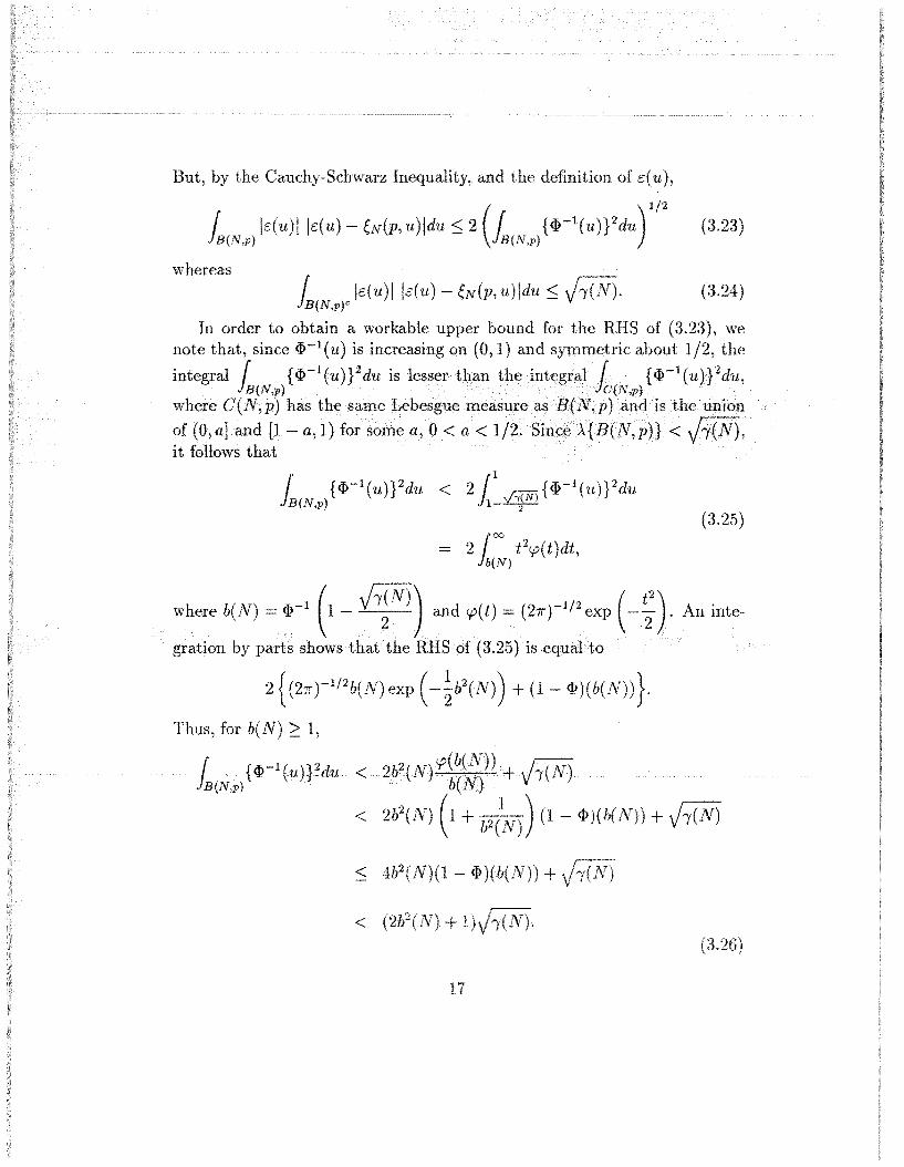
But, the 'Jal1ch:V-;:)lch,,,rarz Ineqm:tlit:y,

k(N,P) le(u)l

[ k(u)1 k(u) - eN(p,u)ldu ~ (3.24)JB(N,p)C

In order to obtain a workable bound for RHS of (3.23), wenote that, since (j)-l(U) is increasing on (0,1) and syrnll1etrlcabout 1/2, theintegral [ {(j)-1(U)}2du {(j)-1

JB(N,p)

'" h""p"" C(N, p) has

of (0, a] and [1 a, 1) forit follows that

2 [00 t 2r.p(t )dt,Jb(N)

(3.25)

where beN) _:-1 (1-~)\and.l'(t) .. (2Jrt1/'.exp (-~) An intec

gration by parts shows that the RHS of (3.25) is equaLto

2 {(211')-1/2b(N)exp (_~b2(N)) + (1- <I>)(b(N))}.

Thus, for beN) 2 1,

<

< 2b2(N) (1 + b2(~V) (1- (j»)(b(N)) +

<

<

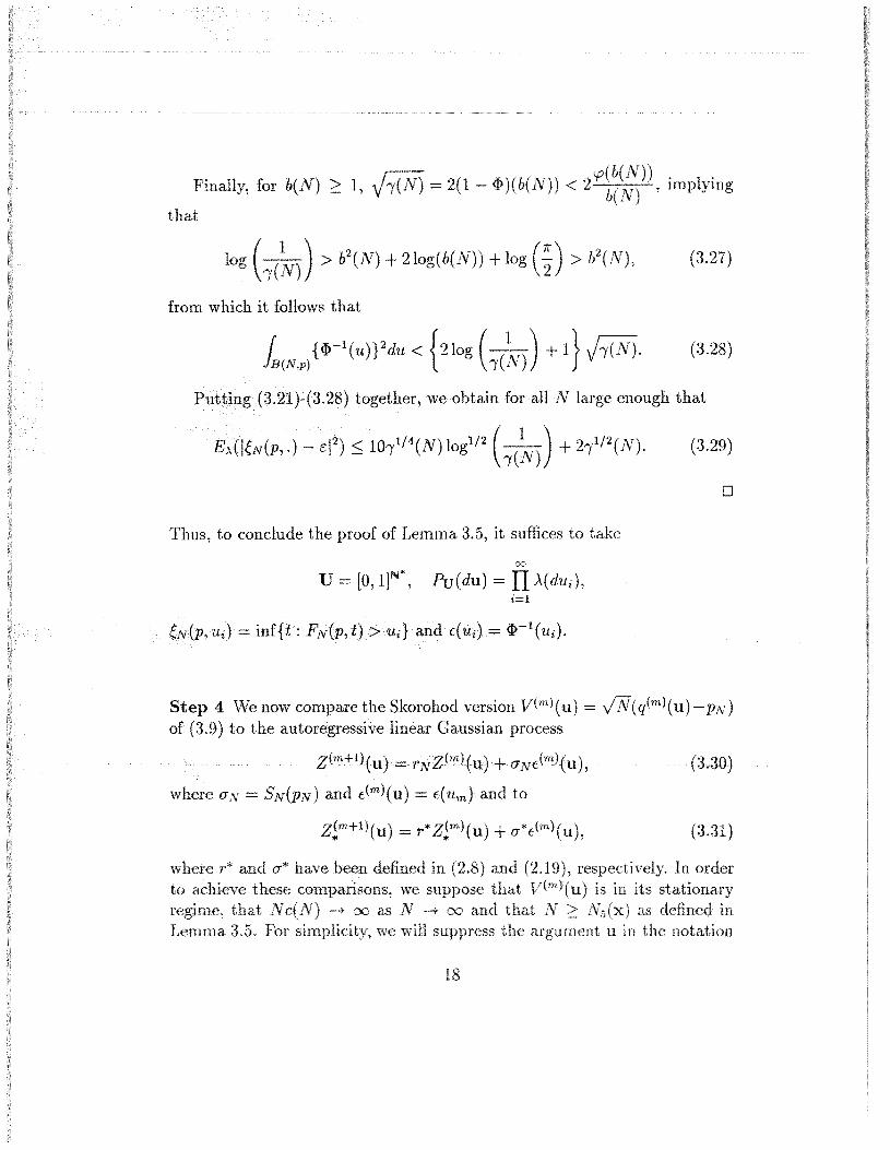
for = 2(1 - <l»)(b(N)) < .:......:..-....:..-:...:.., implying

from which it follows that

Puttin1! (3.21)-(3.28) together, we obtain for all N large enough that

E).(leN(p,.) 61 2) ~ 1O,1/4(N) logl/2 (,(~)) + 2,1/2(N). (3.29)

o

Thus, to conclude the proof of Lemma 3.5, it suffices to take

00

]N· ) IIU [0,1 , Pu(du = >'(dUi),i=l

Step 4 We now compare the Skorohod version v(m)(u) VN(q(m)(U)-PN)of (3.9) to the autoregressive Gaussian Dro,cess

where O'N = SN(PN) and c(m)(u) = c(um) to

r*z~m)(u) o*c(m)(u),

(3.30)

(3.31 )

and write = eN(q(m), um)'

From Lemmas 3.3 and 3,4 it follows that

which implies

(3.32)

II v(m+l) - z(m+l) 112 :S rN II v(m) z(m) 112 +a(N), (3.33)

where

Aoa(N) = --=:::-1---R-(-N-n-2 + (3.34)

with

PN = Ot//8 (N)logl/4 (I(~))}'

If we select Z(O) = V(O), it follows from (3.33) that

(3.35)

II v(m) z(m) II < a(N)2 - 1 'rN

(3.36)

withm

z(m) = (rN)(m)v(o) +aN I:(rN)m-jC;U).

j=l

(3.37)

If, moreover, we select Z£O) = Z(O) V(O), we obtain from (3.30)-(3.31) and(3.33)

where

c *. ( (r*)m8(m,N) = IrN - r I 1- R(N) + 1- r* + IaN - a*l·

(3.38)

(3.39)

if we enouJ!:h an mt(~.e:er

- --.::---:..-- ~ 0 as ~ 00

we obtam a r. v. with

meN)(J* L

i=l

with mean 0 and variance v*{1 (r*)2m(N)}, such that

(3.41 )

(3.42)

can be assume that

'5: a(N), (3.43)

where

and

(3.44)

(3.45)

deduce from the results obtainedfrom which the

L In view of (3.42)-(3.45) and the convergence in distribution of ZN toa from Lemma

dlstfll)utlon to the same

2.

by m meN). Thus

(AN) PNI < {IEu(ZN) II }

< N-1!2 II VN - ZN (3.47)

< N- 1!2a(N),

since ZN has mean 0 and by making use of the Cauchy-Schwarz In­equality. It can be proved similarly that

v* 1lVar (AN) - N l = o(N) (3.48)

provided that the rate of convergence of c(N) to 0 is such that a(N) / {1­R(N)} converges to O.Similar bounds can be derived for higher moments.

3. Let QN(t) = Pu{q(m) :s; t} be the distribution function of q(m) in its

stationary regime and <Pm,N(t) = PU{PN + z:m :s; t}.From (3.36) and Chebyschev Inequality it results that, for all real t andpositive h,

~ 1 [a(N)] 2lQN(t) - <Pm,N(t +h)l :s; h2 1 _ rN (3.49)

Letting m -> 00, we obtain that, for all real t,

IQN(t) - <l>N(t)l 0: :' [t~~~]'+ h ( hSUP

h 4'N)' (3.50)[t- ,jFi,t+ ,jFi]

where (PN(t) is the normal distribution function with andvariance O":F-r/{N(1 r:F-r)} and 4'N(t) is the corresponding density. Aproper selection of h = hN in (3.50) yields for the sup-norm II QN(PN

II < {as -> 00.

4.

as -----t 00. (3.52)

~k()rollOd reI>rel>entation of and ,assuming that q(O) = E JN. Let ke(1! ;::: 1) denote the I! th exit time ofp(m+~) from IN. For 0 ~ m ~ kllq(m) - p(m) and q(k1+1) p(k1+!) 1. IN.

Since TN(q) = j(N)/N E IN and SN(q) = 0 for q 1. IN, q(k1 +2) = j(N)/N.Also, since p(k1 +1) is drawn from rN and rN is assumed to be the Diracmeasure at j(N)/N, p(k1 +1) = q(k1+2) = j(N)/N. An induction shows that,for I! ;::: 0,

(3.53)

1, is theindicator function of Be I N , then there exists m' ~ m such that IB(p(m

/))

1, implying that

for But,

(3.54)

(3.55)

in view of points and (3) Part 1.are in [0,1), (3.56) implies that

I Mean(ll'N) < J; t I ll'N - I (dt)= Oc,ZtV)),

and, similarly,

(3.57)

o;2(N)IVar(ll'N)-Var(AN)I=O( N ), (3.58)

thus (ii) is obtained from point (2), which completes the proof of Theorem1.0

4 Sequential Versions of SEM

In this section, we turn our attention to two different sequential versions ofSEM. Sequential procedures are used when the observations Xl, .•• ,Xn , ... arereceived one at a time and the estimation of the mixture parameters have tobe updated before the next observation is received. The Chapter 6 in Titter­ington, Smith and Makov (1985) provides a thorough examination of sequan­tial methods in the mixture setting. Great attention is paid to the particularproblem of estimating the mixing proportion p* for two-component mixtureswhere the component densities are assumed known. This is the problem that

and Schwartz, 1970), the Quasi-Bayes method (Makov and Smith, , theprobabilistic editor method (e.g., Owen, 197,5), the method of mom~nts (e.g.,

Basu, 1976), a Newton-Raphson-type gradient al,12;Ol'ltnJIIlITlinimum of Kullback-Leibler dlverg:en(~e

prcrbal)11l:3tlC tea,cn(~r method

Subsection 4.1 below. Mc,re()ver, Titteringtona 1!.erlena.l r(~cu:rSl\re method which, particular mlxtlue pr()bl,emCOllsllieratlon, can as

As noted in Titterington et al. (1985), p. toapproach study of asymptotic of vanous proposedprocedures is through the theory of stochastic exploitsthe martingale strucure implicit recursions involved methods"(see (4.1), for instance). Thus, the consistency derived fromthe Quasi-Bayes method, the Kazakos algorithm, the probabilistic teachermethod and the Titterington algorithm have been proved using results frommartingale theory.

A good measure of the efficiency of a sequence of estimators {p(m)} is itsasymptotic relative efficiency defined as

(4.2)ARE 1. mV*1m -::-:---:--:--:-::-

n->oo Var(p(m»)

where V* = J;b; is the Cramer-Rao lower bound. Kazakos (1977) has de­signed his algorithm to be fully efficient, i.e. to have ARE = 1. But hisscheme requires numerical integration which are computationnally unattrac­tive. Now, it is a striking fact that the ARE's of the Quasi-Bayes, the prob­abilistic teacher and the Titterington algorithms are positive iff the ratioJobs / Jc > 1/2.

4.1 The one-step sequential SEM algorithm

This is the standard sequential version of SEM. time a new observationXm+l is received, only the classification Zm+l is drawn at random from thecurrent posterior probability t(Xm+bp(m»). There is no feedback as to thecorrectness of previous decisions: The other z(i)'s, 1 ::s j ::s m, are con-stant. More formally sequential SEM works as follows.by p(m)(m ~ 1) the estimate of computed on the oftions Xl, •.. ,

has been received,= t(xm+l,p(m»), according to (2.3).

from a Bernoulli distribution with paralneteras

+----­m+1

are SUlnnlar'izE~d

--1' p* a.s. as m --1' 00.

algorithm is equal toTheorem 2

ARE of the one-step sequenhal

(Jc

ARE = max 0,2 - -J )obs

(4.4)

4.2 The global sequential SEM algorithm

8UI>sectl1on, we 2 and 3. The mainTheorem 3. This theorem

paJrtl(:Ulct.r sequential version of SEMcall the This version works as fol-

lows. Denote by p(m)(m ~ 1) the estimate of p* computed on the basis of theobservations Xl, ..• ,Xm and by p(O) the starting point of the algorithm. Afterthe (m + l)th observation, Xm+b has been recorded, the E-step updates theposterior probabilities as t}m+l) = t(Xi,p(m»), i = 1, ... , m, and computes the

new posterior probability t!:+~l) = t(Xm+bp(m)), according to (2.3). The S­

step draws independently each r.v. z}m+l), i = 1, ... , m + 1, from a Bernoullidistribution with parameter t}m+l). The M-step updates pm as

where e(m+l) = em+l (p(m) , w(m+l)).The important difference with the one-step sequential SEM algorithm is

that all the observatioIls are attributed to one of the compo-nents of mixture has been recorded. Accord-

lnt,prV'::l.l~ Jm. This means choice pCm)from Jm is not important. This is the reason

of the procedure implicitly contained in (4.5): It isproving Theorem 3, following our approach.

Theorem 3 (i) asserts that, under assumptions which (Hl)-(H4)above, the Po - distribution of pCm) = pCm)(x,w) is Px - a.s. asymptoticallynormal with mean pm and variance v*m-1, where = Pm(x) is the MLestimate of p* based on the sample {XI, ... ,xm} and = (0-*)2{1- (r*)2}-1,with r* and 0-* defined in (2.8) and (2.19), respectively.

Theorem 3 (ii) provides Px- a.s. asymptotic upper bounds for IEo(p(m»)­Pml and IVaro(pCm») - v*m-11. These bounds make (i) more precise.

Before stating Theorem 3, we need to state assumptions (H5) and(H6), which are as follows.(H5) For Px- a.e.x, Em~lm-2{1 - R(m)}-4 < 00 and Em~lm-l,B2([OmJ)<00 for any 0,0 < 0 < 1, where [tJ denotes the largest integer:::; t.(H6) There exists an exponent 1t,0:::; It < 1, such that m-/l = O(c(m)). (ForIt = 0, this means that c(m) is constant. Note that (H6) implies (H2).)Finally, recall that £(m) = {2£2(m)}1/2, where £2(m) denotes the iteratedlogarithm. We can now state Theorem 3.

Theorem 3 (i) Suppose that the assumptions (Hi), (H3}-(H4) and (H6)hold. Then, m1/2 (pCm) - Pm) converges Px - a.s. in Po - distributionto a Gaussian r. v. with mean 0 and variance v*.

(ii) Under the assumptions (Hi), (H3}-(H4) and (H6), f01' Px - a.e. x andall m large enough,

and

IVar~2(pCm») - m-1/2 (v*)1/21:::; 2m-I/2aSeq(m) +O(m-1£(m)), (4.7)

where, for all 0,0 < 0 < I,

(m) O(,B([OmJ)) +O(m-1/2{1 - (4.8)

o - a.s.

lim a.s. 10)

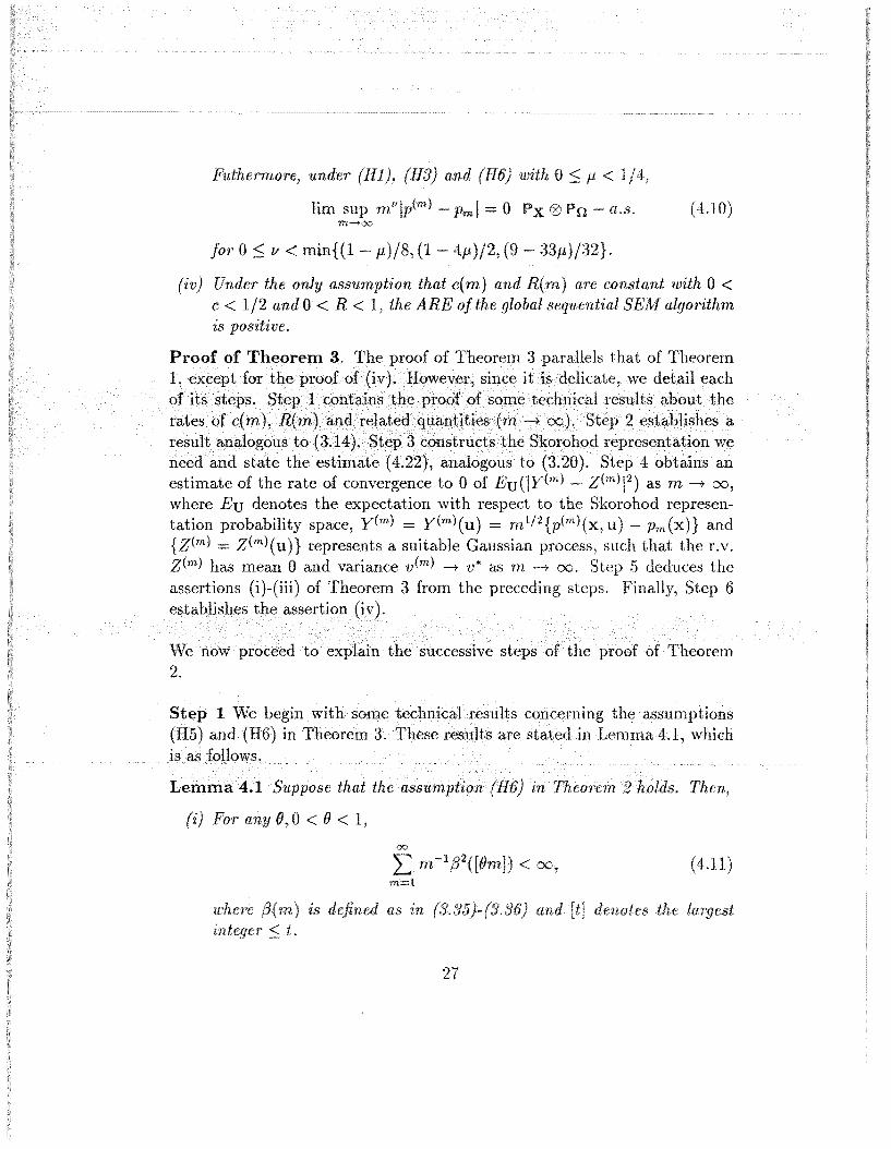
for 0 S 1/ < min{(1 - p,)/8, (1 -

(iv) Under the only assumption that c(m) and are constant with 0 <c < 1/2 andO < R < 1, the of the global sequential SEM algorithmis positive.

UUI,(;I,111::> anestimate of the rate of convergence to 0 - z(m)12) as m --t 00,

where Eu denotes the expectation with respect to the Skorohod represen­tation probability space, y(m) y(m)(u) m1/ 2 {p(m)(x, u) - Pm(x)} and{z(m) = z(m)(u)} represents a suitable Gaussian process, such that the r.v.z(m) has mean 0 and variance v(m) --t v* as m --t 00. Step 5 deduces theassertions (i)-(iii) of Theorem 3 from the preceding steps. Finally, Step 6

2.

Step 1 begin(U5) and (H6)

Theorem

which

Suppose that

(i) 6,0 < (j < 1,

Then,

m=l<

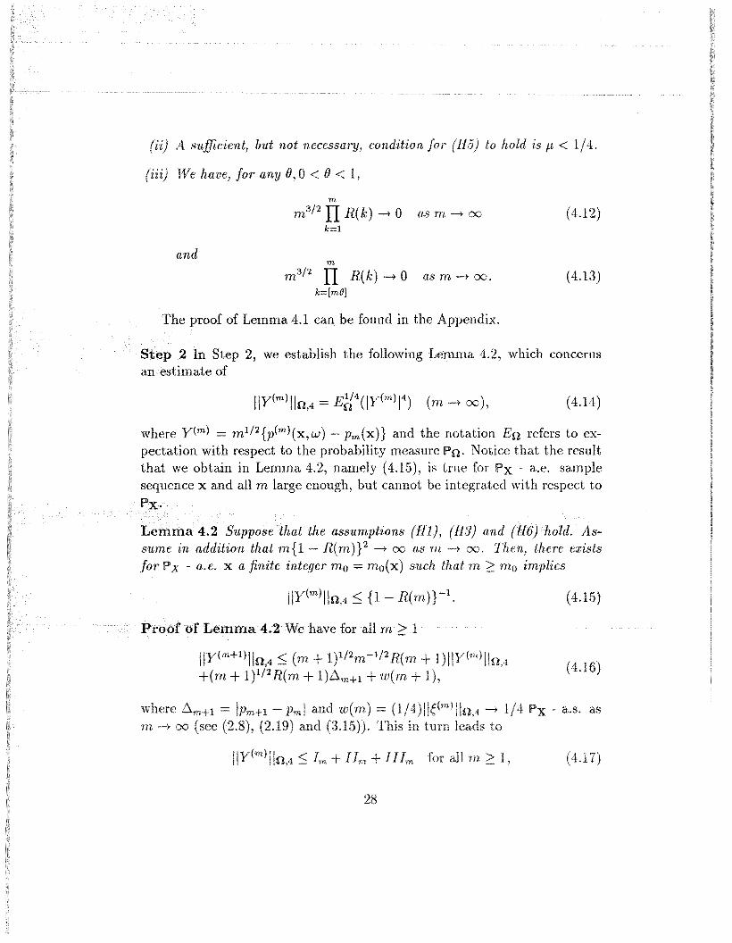
A sUI!JLczen,t, but not ne(~es~,ary, condition for to hold is p < 1/4.

for any 0,0 < 0 < 1,

m

m 3/

2 IT R(k) -+ 0 as m -+ 00

k=l

(4.12)

andm

m 3/2 IT R(k) -+ 0 as m -+ 00.

k=[m8]

The proof of Lemma 4.1 can be found in the Appendix.

(4.13)

Step 2 In Step 2, we establish the following Lemma 4.2, which concernsan estimate of

(4.14)

where y(m) = m 1/ 2 {p(m)(x,w) - Pm (x)} and the notation Eo refers to ex­pectation with respect to the probability measure Po. Notice that the resultthat we obtain in Lemma 4.2, namely (4.15), is true for Px - a.e. samplesequence x and all m large enough, but cannot be integrated with respect to

LetUIl1la 4.2 Supposethat the assumptions (Hl), (H3) and (H6) hold. As­sume in addition that m{1 - R(m)}2 -+ 00 as m -+ 00. Then, there existsfor Px - a.e. x a finite integer mo = mo(x) such that m ::::: mo implies

(4.15)

Proof of Lemma 4.2 We have for all m ::::: 1

lIy (m+l)lIo,4::; (m +1)1/2m-1/2R(m + I)! 110,41)1/2R(m 1)~m+l +w(m +1),

-+ 1 - a.s. asto

< +

where 110,4 = m 1,

m

- m1/22:ITm(j)Lljj=2

m

2:(mfj)l/2ITm(j + l)w(j),j=2

(4.18)

1, ... ,m, with the convention that

1) for j = 1, ... , m and,mt€~,2;er m1 = m1 (x)

splIttUt,2; intoITm(j)Llj,m 2:: m2:

and ITm(j) = R(j) ... R(m) for jITm(m 1) = 1.

Since R(j) ~ R(j + 1) for j 2:: 1, ITm(j) ~ ITm(jby Lemma AA in the Appendix,such that m 2:: m1 Llm ~

Em, with Am = m1/2E~;5j;5[8m]ITm(j)Llj and Emwhere 0 < () < 1 and [t] denotes the largest integer ~ t,

[8m]I 1m ~ m1/22:ITm([(}mD + m1/2(2Jc/ Jobs) [(}m]-l

j=2(1 + R(m) + R2(m) + ... )

< m3/ 2ITm ([(}mD +m-1/2(}-1(2Jc/Jobs){1 - R(m)}-l- 0(1)

(4.19)

in view of (H6) and Lemrna 4.1. Splitting 111m similarly provides

[8m]I I 1m ~ (m/2)1/2ITm ([(}m] + 1)[(}mj[(}mJ-l 2:w(j)

j=2+(m/[(}mD1/2(maxrBm];5j;5m w(j))(l + R(m) + ... )

(4.20)

< m3/ 2 ITm ([(}m] l)[(}m]-l

U.L""''''[tfmlSJ''"m w(j)).

+ (}-1/2{1 _ R(m)}-l

asm-+oo

< + -1 )

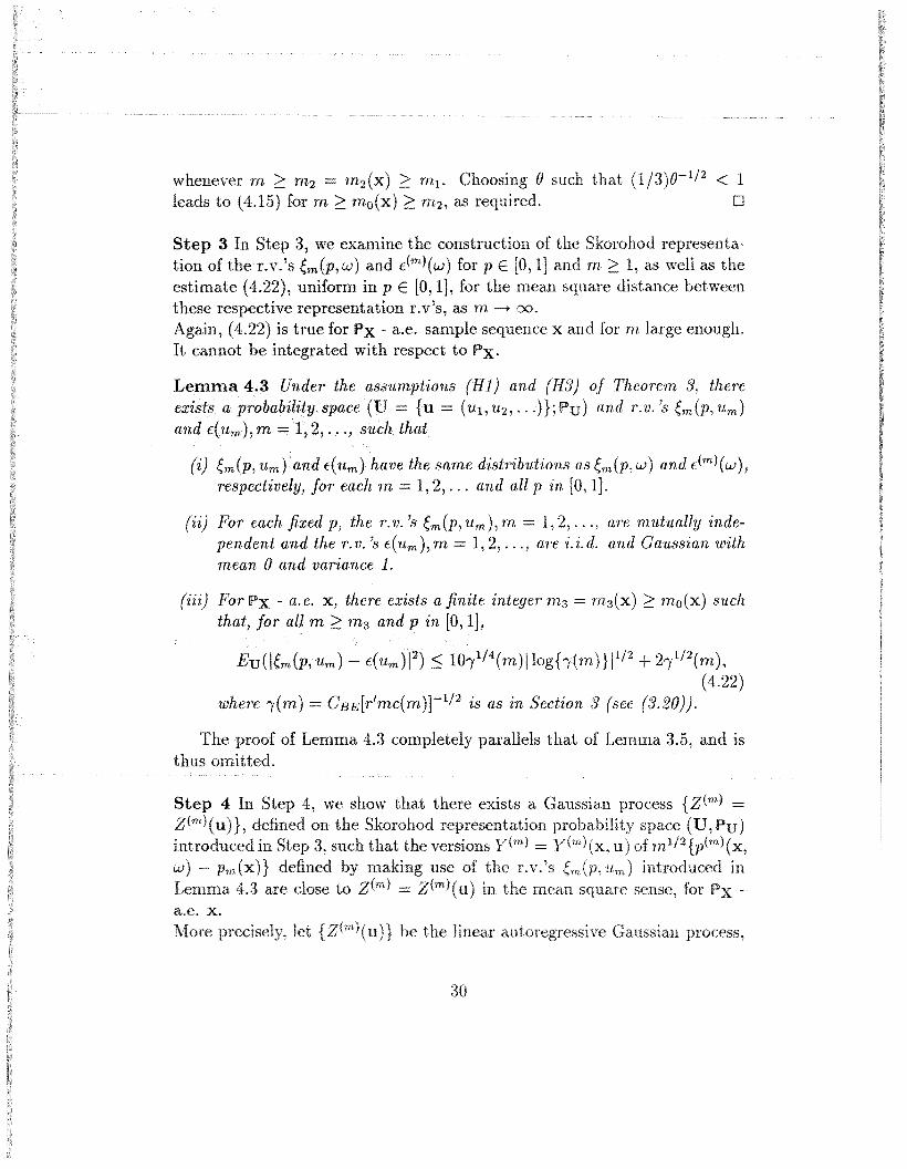
wbLeneV(~r m 2:: m2 m2 (x) 2:: mI' Choosing 0to (4.15) m 2:: mo(x) 2:: m2, as required.

(1/3)O-I/2 < 1o

Step 3 In Step 3, we examine construction of the Skorohod representa-of r.v.'s ern(P,w) c(m)(w) for p E [0,1] and m 1, as well as the

estimate (4.22), uniform in p E [0,1], for the mean square distance betweenthese respective representation r.v's, as m -+ 00.

Again, (4.22) is true for Px - a.e. sample sequence x and for m large enough.It cannot be integrated with respect to Px.

Lemma 4.3 Under the assumptions (H1) and (H3) of Theorem 3, thereexists aprobabilitYf3pace (U = {u = (Ul,U2"")};pu) and l'.V.'S ern(P,urn )and c:(urn }, m 1,2, ..., such that

(i) ern (p, Urn) and c:(urn) have the same distributions as em(p, w) and c:(rn) (w),respectively, for each m = 1,2, ... and all p in [0,1].

(ii) For each fixed p, the r.v. '13 ern(P, urn), m = 1,2, ... , are mutually inde­pendent and the r.v. '13 c:(urn ), m = 1,2, ... , are i.i.d. and Gaussian withmean 0 and variance 1.

(iii) For Px - a.e. x, there exists a finite integer m3 = m3(x) 2:: mo(x) suchthat, for all m 2:: m3 and p in [0,1],

Eu(lern(P, urn) c:(urn )12):::; lO,I/4(m)llog{,(m)}II/2+ 2,1/2(m),(4.22)

where ,(m) CBE[r'mc(m)t l/

2 is as in Section 3 (see (8.20)).

The proof of Lemma 4.3 completely parallels that of Lemma 3.5, and isthus omitted.

Step 4 In Step we show that there exists a Gaussian process {z(m) =z(m)(u)}, on the Skorohod probability (U,pu)introduced in 3, that the (x,u)ofm l / 2{p(rn)(x,

(x)} defined by urn) into mean

a.e. x.

defined on (U, pu) by the recursion formula

z(m+l)(u) = + (u) + c(m+l)(u)

with Z(l)(U) O"lC(l)(U). Then,

m 2:: 1, (4.23)

m

z(m)(u) = IJmjj)1/21rm(j + l)O"jc(j)(u) for m 2:: 1,j=l

(4.24)

where 1rm(j) = rj ... rm for j 1, ... , m and 1rm(m + 1) = 1, is a Gaussianr.v. with mean 0 and variance

m

v(m) = ~(mjj)1r;'(j + 1)0"}-j=l

(4.25)

(4.26)

Moreover, define y(m)(x, u) = m1/ 2{p(m)(x, u)-Pm(X)}, where p(O) (x, u)p(O) and, for m 2:: 0,

p(m+l)(x, u) = Tm+dp(m)(x, u)} + (m +1t1/ 2

8m+l {p(m)(x, u)}e(m+l)(x, u),

where e(m+l) (x, u) = em+l {p(m)(x, u), um+d.In the sequel, we will suppress the notation indicatiI~ the dependence on

u or (x, u), unless necessary. We will let IIYllu,O' = Eh O'(IYIO') for all finitea 2:: 1.

Lemma 4.4 below provides an estimate for Eu(ly(m) - z(m)1 2 ) as m -1­

00. This estimate is uniform in p E [0,1J and is true for Px - a.e. x.Unfortunately, the integration of inequality (4.27) with respect to Px doesnot lead to a similar estimate.

Lemma 4.5 below shows that the variance v(m) of z(m) converges to v* asm -1- 00 and provides an estimate for Iv(m) - v*l.

Lemma is as follows.

Lemma 4.4 Under the assumptions (H1), (H3) and (H6) and the additionalassumption m{l - R(m)}4 -1- 00 as m -1- 00, the uniform (in p) Skorohodrepresentations y(m) and z(m) satisfy Px - a.s.

(4.27)- z(m)lIu,2 :::;

0,0<0<1,

1-+

for all m

31

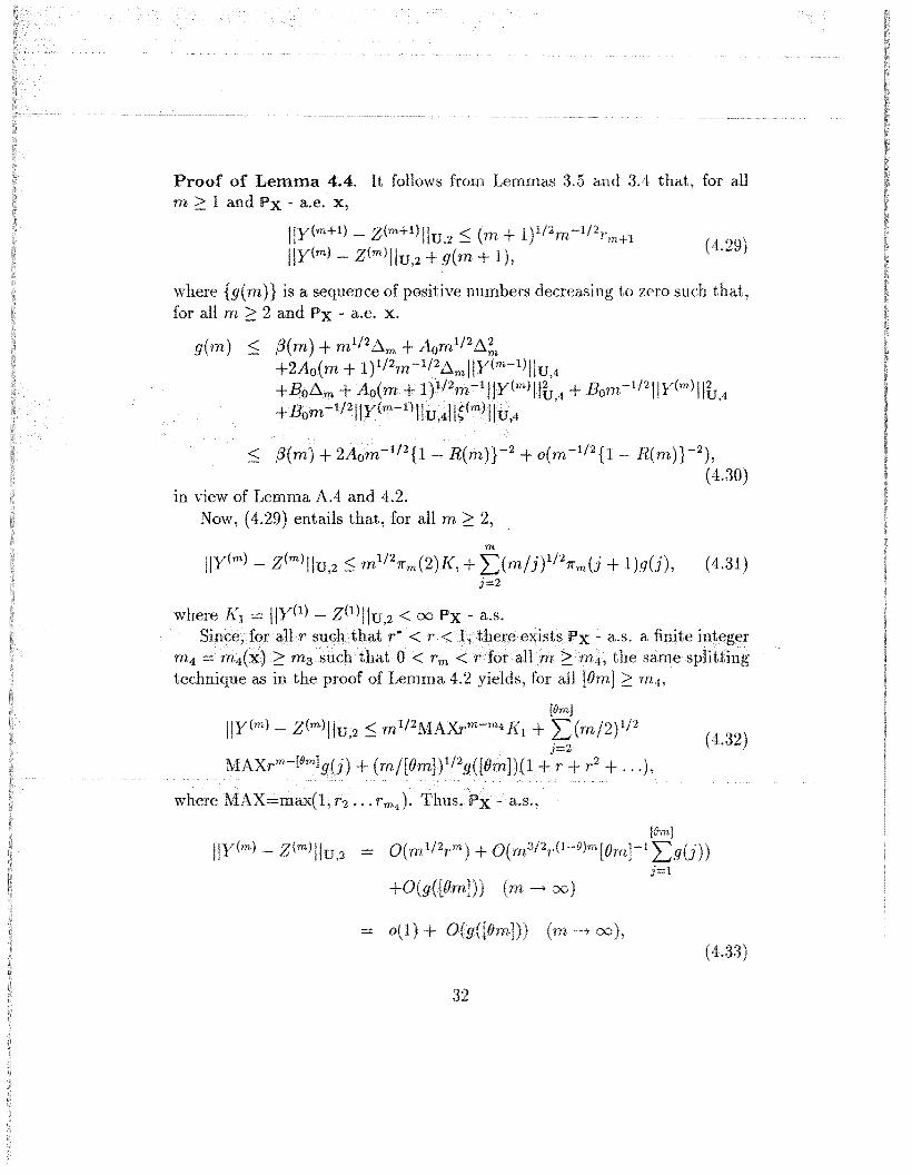
Proof of Lemma 4.4.m ;:::: 1 Px - a.e. x,

Lem.mas 3.5 3.4 that, for all

(4.29)

where {g(m)} is a of positive numbers decreasing to zero such that,for all m ;:::: 2 and Px - a.e. x.

g(m) ~ tJ(m) + ml/2~m Aoml/2~~

+ 1)1/2m-l/2~mlly(m-l) lu,4IHJ,4 Bom-1

/2 11y(m)llb,4

< tJ(m) +2Aom-1/ 2{1- R(m)}-2 +o(m-1/ 2 {1 - R(m)}-2),(4.30)

in view of Lemma AA and 4.2.Now, (4.29) entails that, for all m 2:: 2,

m

lIy(m) - z(m)llu,2 ~ m1/21l'm(2)I<,+ '2:Jmfj)1/21l'm(j + 1)g(j), (4.31)j=2

(4.32)

where I<l = lly(l) - Z(1)l!U,2 < 00 Px - a.s.such .that r* < - a.s. a finite integer

m4 = mgsuch that 0 < rm the same splittingtechnique as in the proof of Lemma 4.2 yields, for all [lJm] ;:::: m,t,

[Om}

lly(m) - z(m)llu,2 ml/2MAXrm-m4 I<l L(mj2)1/2j=2

r +...),where

[8m}

Lg(j))j=l

(4.27)-(4.28), in view of (4.30), as required. o

vVe now turn to Lemma 4.5.

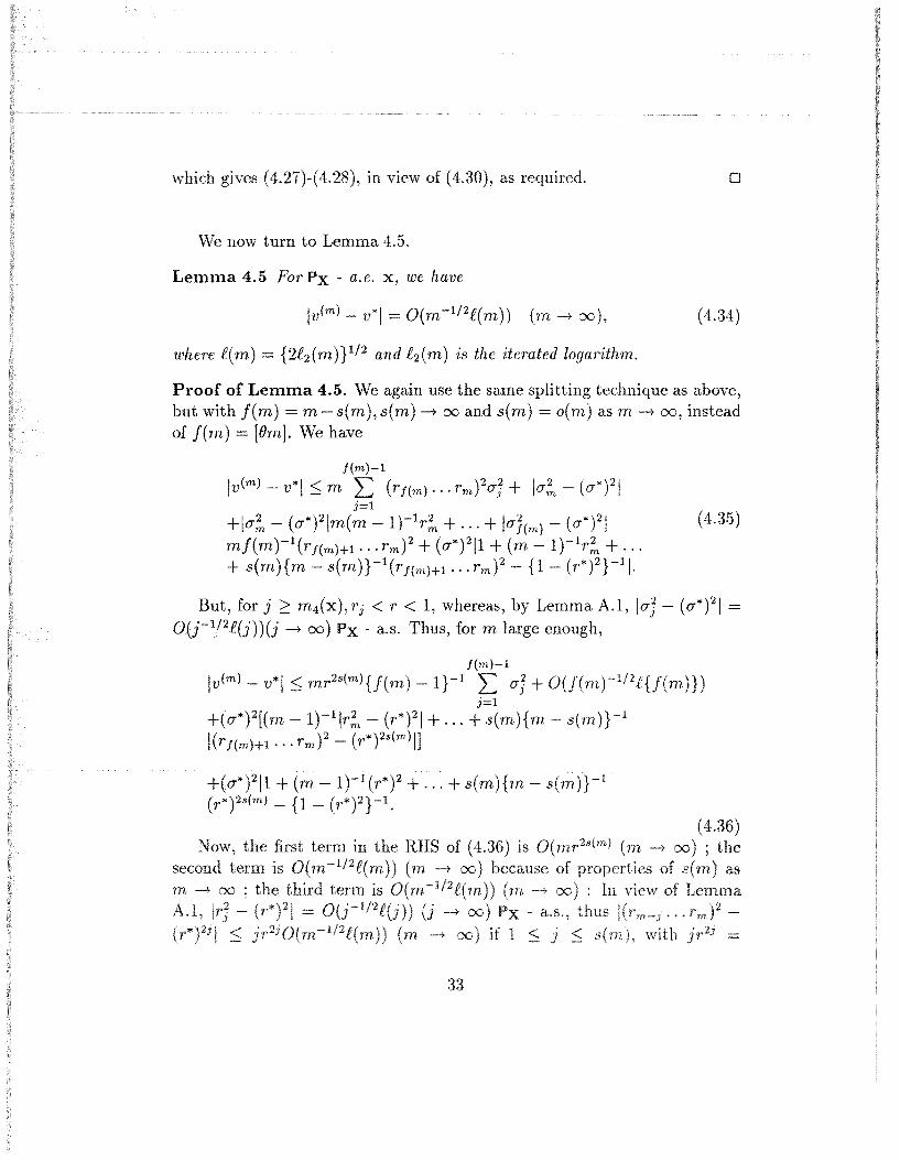
Lemma 4.5 For Px - a.e. x, we have

Iv(m) - v*1 = O(m-1/2£(m)) (m -+ (0),

where £(m) = {2£2(m)}1/2 and £2(m) is the ite1'ated logarithm.

(4.34)

+(17*)211 + (m(r*)2s(m) {I

Proof of Lemma 4.5. We again use the same splitting technique as above,but with f(m) = m-s(m),s(m) -+ 00 and s(m) o(m) as m -+ 00, insteadof f(m) [Om]. We have

f(m)-lIv(m) - v*1 :; m L (rf(m)'" rm)2o} + 117~ - (17*)21

j=l

+117~ (17*)2Im(m - 1)-lr~ + ... + I17J(m) - (17*)21 (4.35)mf(m)-l(rf(m)+l" .rm)2 + (17*)211 + (m - 1)-lr~ + ...+ s(m){m s(m)}-l(rf(m)+l" .rm)2 - {1- (r*)2}-11.

But, for j 2': m4(x), rj < r < 1, whereas, by Lemma A.l, I17J (17*)21 =O(j-l/2£(j))(j -+ (0) Px - a.s. Thus, for m large enough,

f(m)-lIv(m) - v*1 :; mr2s(m){f(m) _1}-1 L 17J +O(f(mt1/ 2£{f(m)})

j=l

+(17*)2[(m 1)-llr~ - (1'*)21 + ... + s(m){m - s(m)}-ll(rf(m)+l'" rm)2 - (r*)2S(m)l]

(4.36)rnv~D\'''1 (m -+ (0) ; the

propertIes of as

j log rlJ} :::; supx>o x... + s(m){m - s(m)}-l :::;

; the is houndedAlog m :::; s(m) = o(m) (m -+ with A >proof. o

Step 5 We are now in a position to deduce the assl~rtlons (i)-(iii) of Theorem2 from Lemmas 4.1-4.5.

Proof of (i):m -+ 00 tothat y(m) con.verlresmean 0 and variam:ein Po distribution. Hence

Proof of (ii): From Lemma 4.4 and the Cauchy-Schwarz inequality, for Px ­a.e. x and all m large enough,

IEu(p(m) - Pm - m-1/ 2z(m»)1 - IEu(p(m») - Pml- IEo(p(m») - Pml< m-1/ 21Iy(m) - z(m)llu,2< m-1/ 2etseq (m).

Hence,

(4.37)

We turn to the variance ofp(m) with respe<:t to Po, Vetro(p(m»).We have for Px - a.e. x and all m large enC)lljil;Jn,

Ilu,2' (4.39)

Thus,

Thus,

and

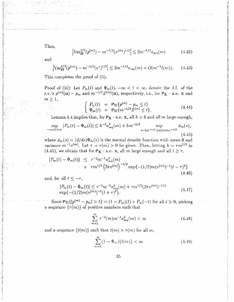
< (4.42)

- m- I / 2(v*)1/21 S 2m-I/2aSeq(m) +O(m-ll(m)). (4.43)

This completes the proof of (ii).

Proof of (iii): Let Pm(t) and ~m(t), -00 < t < 00, denote the dJ. of ther.v. 's p(m)(u) - pm and m-I / 2 z(m)(u), respectively, Le., for Px - a.e. x andm 21,

{Pm(t) pu{p(m) Pm S t}

··.~m(t) = Pu{m-I / 2z(m) S t}. (4.44)

LeIllIIlla 4.4 implies that, for Px - a.e. x, all h > 0 and all m large enough,

sup IPm(t) ~m(t)1 S h-2a;eq(m) + hm- I/

2 sup <Pm(s),-oo<t<oo t-hm -liZ <s<t+hm- l / Z

- - (4.45)

where <Pm(s) = (d/ds)~m(s) is the normal density function with mean 0 andvariance m-1v(m). Let T = T(m) > 0 be given. Then, letting h = Tml / 2 in(4.45), we obtain that for Px - a.e. x, all m large enough and all t 2 T,

and, for all t S -T,

(t) - ~m(t)1

-(1/2)m(v(mlt1 ( t

a seqiUe][lce

a;eq(m) +Tml / 2(27rv(m)t1!2

T)2}. (4.47)

0, pICfanp;

L T-2(m)m- 1a;eq(m) < 00

m=l

(4.48)

a seq:uel1ce > Tn,

<00

L r(m)m1/

2 exp[-(1/2)m(v(m)t1 {t(m) - r(m) < 00

m=l

yields, in view of (4.46)-(4.47),

Pu{lim sup C1(m)lp(m) - Pml :s; I} = 1 Px - a.s.m ......oo

It is possible to choose

t(m) = cst.m-v

for any positive constant cst. and

o :s; 1/ < min{(l - f-L)/8, (1 - 4f-L)/2, (9 - 33f-L)/32}.

For (H6) with f-L = 0 (i.e., c(m) = constant), it is possible to choose

t(m) cst.m-1/ 8

for any positive constant cst. This concludes the proof of (iii).

(4.50)

(4.51 )

(4.52)

(4.53)

(4.M)

Step 6 In this last step, we consider the ARE of the global sequential SEMalgorithm and prove assertion (iv) of Theorem 3. This is the subject of thefollowing lemma.

Lemma 4.6 Under the ass'umption that c(m) = cR = constant, with 0 < c < 1/2 and 0 < R < ,sequential SEM algorithm is positive.

Proof of Lemma 4.6 It suffices to show that

constant and R(m) =ARE of the global

E( (4..55)

1).

12 1Fm ) E{+(m+

< Pm+112IFm)+(1/2)(m + 1)-1 a.s.

< R2 Ip(m) Pm 12 + E(IPm+l Pm1 2 1Fm)

+2E(lp(m) - PmlIPm+1 - PmlIFm)+(1/2)(m + 1)-1 a.s.

< R2Jp(m) - Pm 12 +E(IPm+1 -PmI2IFm)

+2Ip(m) - PmIEl/2(IPm+1 - Pm121Fm)+(1/2)(m +1)-1 a.s.

(4.56)If we take the expectation of both members of (4.56), we obtain, by

making use of the Cauchy-Schwarz inequality,

IIp(m+1) - Pm+111~ ::; R21Ip(m) - Pmm IIPm+1 Pmll~

+211pm Pmll2l1Pm+l - Pm 112 + (1/2)(m + It1.(4.57)

Now, since Pm is the ML estimate of 1'* based on {Xl,"" X m}, we haveIIPm = Eflp"..--p*1)2 rv (rnJobs)-l as m Thus, for any 1/0 > 0,there exists a finite integer M(vo) such that m .~ implies

IIp(m+1) - Pm+1m ::; R211p(m) - Pmm +4(1 + vo)1/2(mJobs )-1/21Ip(m) - Pmlb1/0)(mJobst l + (1/2)m-1.

If we define

(4.58)

2(1 vot l / 2J~;/2, B(vo) = B = 2(1 +vo)J;b; +

Y2 < R2y2 +2Am-1/2y Bm-1m+l - m m (4.59)

there exists an mt('~g:er

m~

some

for all m ~ Al(vo). 'lie now prove inductionNfl a constant I< such

<

<

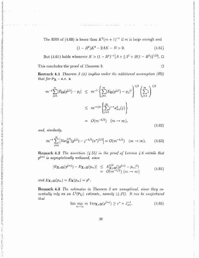
The RHS of (4.60) is lesser than K 2 (m + if m is

- R2 )K2- 2AK B > O.

enough and

(4.61 )

This concludes the proof of Theorem 3. o

Remark 4.1 Theorem 3 (ii) implies under the additional assumption (H5)that for Px - a. e. x

(4.62)and, similarly,

m

m-1 L IVar~2(p(j)) - j-1/2(v*)1/21 = 0(m-1/ 2 ) (m -+ (0). (4.63)j=1

Remark 4.2 The assertion (4.55) in the proof of Lemma 406 entails thatp(m) is asymptotically unbiased, since

IExxn(p(m)) - EXxo(Pm)1 < Ei'~o(lp(m) - Pm1 2)

= 0(m-1/ 2 ) (m-+oo)(4.64)

Remark 4.3 The estimates in Theorem 3 are nonoptimal, since they es­sentially rely on an L2(pu) estimate, namely 27). It can be conjecturedthat

m Varxxo ) 2:: +

SarnpJle fluctuationsasymptotically

We now try supportand (4.43) that Eo(lp(m) - Pm12) =

SUPm mExxo(lp(m) - 12) ~ImplH~S that limsuPm p*12) =of m1/ 2(Pm-P*) and m1

/2{Eo(p(m»)-Pm} can

uncorrelated : indeed,

IEx xo{m-1/ 2(Pm - p*)D(m)}1 < Ex(m1/2IPm - p*IIID(m)llo,2)

< E:¥2(mIPm p*12) IID(m)llxxo,2- O(llD(m)llxxo,2) (m -+ (0).

(4.66)where D(m) y(m) _ z(m).

Now it can he expected .that Ily(m) - z(m)llxxo,2 -+ 0 as m -+ 00.

But, since z(m) has Po me(;ill 0, Exxo{m1/ 2(Pm - p*)(y(m) - z(m»)} =Exxo{m1/ 2(Pm - p*)y(m)}, with y(m) = m1/ 2(p(m) Pm). From a heuristicpoint of view, (4.65) tells us that the variance of p(m)(x,w) can be splitinto the variance of pm and the variance of the fluctuations related to thesimulation S-step, the latter being of a magnitude ~ v*m-1 as m -+ 00.

Recalling that v* J;;{1 + (Jc/Jcond)}-l < (2Jobst\ the conjecture (4.65)would imply, if it were true, that the ARE of the global sequential SEMalgorithm is :::; [1 + {1 + (Jc/Jcond)}-ltl. If, furthermore, the inequality

(4.65) could be replaced by equality, then the ARE would be > 2/3 andwbuldconverge to 1 as Jobs/Jc converges 1, the mixture becomesmore and more separable.

Remark 4.4 As for the one-step sequential SEM algorithm, the global se­quential SEM algorithm can be considered as a sequential Bayesian algorithm.Here, the underlying Bayesian algorithm is Tanner and lVong's (1987) one.

the mixture has [{ ~ 3 components is straightforward.

Remark 4.6 for Theorem 1,has

APPENDIX

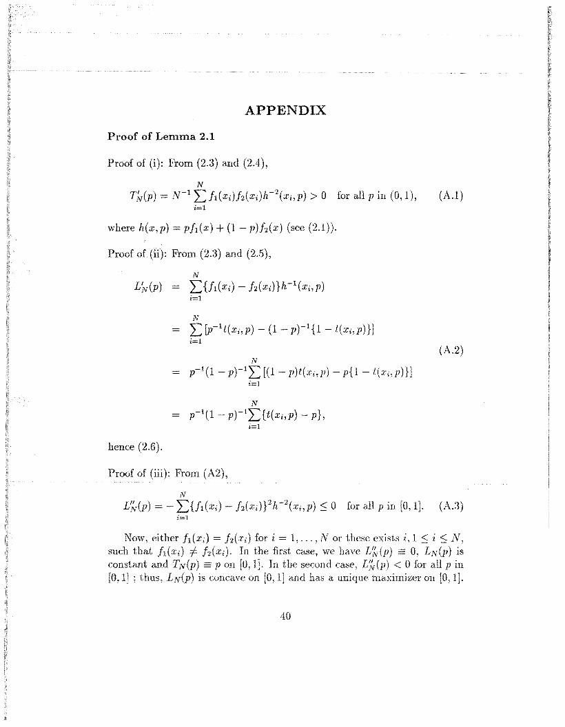
Proof of Lemma 2.1

Proof of (i): (2.3) and (2.4),

N

r.i.,(p) = N-1 'L!I(xi)h(Xi)h-2(Xi,p) > 0 for all p in (0,1), (A.l)i=l

where h(x,p) = pfl(X) + (1 - P)f2(X) (see (2.1)).

Proof From (2.3) and (2.5),

N

LN(p) 'L{!I(Xi) - h(Xi)}h-1(Xi,p)i=l

N

- 'L [p-lt(Xi,p) - (1 - pt1{1 - t(Xi,p)}Ji=l

(A.2)N

- p-l(1 - pt1'L [(1 - p)t(Xi,p) - p{1 - t(;1;i,p)}Ji=l

N

_ p-l(1- p)-l'L{t(Xi'p) p},i=l

hence (2.6).

Proof of (iii): From (A2),

N

L';v(p) = - 'L{!I(Xi) - h(Xi)}2h-2(Xi,p) ::; 0 for all p in (O,IJ. (A.3)i=l

i,1 ::; i ::; N,=0, LN(p) is<0 p

J:urthe:rmore for all x in and P in (0,1),

p)}2p) ::::; 1).

(AA)Thus, the SLLN implies that for Px - a.e. x in X and all P in (0,1)

{f1(X) - h(x)}2h-2(x,p) < p) + 1< 2{p-2+ (1 _ p)-2}

1'1-1Ljv(p) -l' L"(p) = J{f1(X) - h(x)}2h-2(x,p)h(x,p*)p(dx)as 1'1 -l' 00.

(A.5)

By the assumptions of Theorem 1, L"(p) < O. Hence (iii).

Proof of (iv) : From (2.6),

Tfv(p)-l = (1-2p)1'1- 1LN(p)+p(1-p)1'1- 1L~v(p) for all pin (0,1). (A.6)

Thus, for p PN, where Ljv(PN) = 0 and Lj:"'(PN) < 0, we have

Tfv(PN) = 1 +PN(l - PN )1'1-1 L'fv(p) < 1. (A.7)

As Tfv(PN) > 0 and TN(PN) = PN again by (2.6), (2.7) is proved.Furthermore, since LN(p) < 0 for all 0 < P < PN and LN(p) > 0 for all

PN < P < 1, the remainder of (iv) obtains again from (2.6). (Compare theproof in Silverman (1980).)

Proof of (v) : Assertion (v) is a direct consequence of (iv) and its proofwill be omitted here.

Proof of (vi) : Remark that the empirical complete-data information valueIN,c = p,,?(l PNt 1 and the empirical observed-data information valueIN,obs = _1'1-1 Lj:"'(PN) (e.g., Titterington et al (1985)). Thus, from (A.7),

(A.8)

Since Jit:JN,obs -l' J;;1 Jobs as 1'1 -l' 00 for Px - a.e. x and J c +(vi) OOl,alIJcS.

It isster al.

COlItpOllent derlsitJleS" (Windham 'Vucv,'~>. (1991(1982) :;undber.a: (1976)) that

algorithm is the lan~est emlgenvaille ofIS coherellt with (vi) above.

Indeed, it is well­of

o

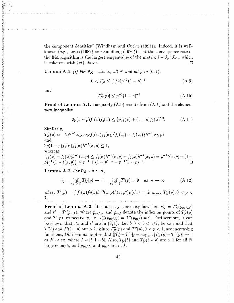
Lemma A.I (i) For Px - a.e. x, all and all p in (0,1),

o< T,~ ::; (1/2)p-l (1 pt1

and

(A.9)

(A.lO)

Proof of Lemma A.I. Inequality (A.9) results from (A.l) and the elemen­tary inequality

(A.ll )

Similarly,TN(p) = -2N-1L,1<i<Nh(Xi)h(Xi){fl(Xi) - h(Xi)}h-3 (Xi,p)and2p(1 - P)fl(X)h(x)h-2 (x,p) ::; 1,whereasIfl(X) - h(x)lh-1(x,p) ::; h(x)h-1(x,p) + h(x)h-1(x,p) = p-1t(x,p) + (1­pt1{1 - t(x,p)} ::; p-l + (1- pt1 p-l(1 - p)-l. 0

Lemma A.2 For Px - a.e. X,

r~ = inf Tfv(p) -+ r' = inf T'(p) > 0 as m -+ 00pE(O,l) pE(O,l)

(A.12)

where T'(p) J fl(x)h(x)h- 2(x,p)h(x,p*)p,(dx) = limN-+oo Tjv(p),O < p <1.

that rN T1V(Pinf,N)inflexion points of T,v(p)

)= O. it canb,O < b <

O<p<l

"~~U.1' ITI~(Pin/,N) - T"(Pin/,N) I IT"(Pin/,N) I :::; IIT~ - Til II I -+ 0 asm -+ 00. Thus, T"(Pin/,N) -+ 0 as N -+ 00, which that -+ Pin/as -+ 00 and r~ = TN(Pin/,N ) -+ r' T'(Pin/) as -+ 00. 0

Lemma A.3 For Px - a.e. x and all N large enough,

where cst. denotes some positive constant.

Proof of Lemma A.3 Since

S~ p-1/2(1 - p)-1/2(1 2p){TN(p)}1/2 + (112)p1/ 2(1 _ p)1/2{TN(p)} -1/2T~(p), (A.14)

we have for all p in (0, 1) that

1Sf¥ (p) 1 :::; (I/2)p-1 (I - pt1 + (l/2)rf¥ -1/2p-3/2(I _ p)-3/2,

in view of (A.9) and (A.lO).

Lemma AA (i) We have

IrN - 1'*1 = O(£(N)N-1/2) (N -+ (0).

(A.I5)

o

(A.16)

(ii) We have(A.I7)

Proof of Lemma AA Proof of (i): From the general theory of ML esti­mation, IPN - p*1 = O(£(N)N-1/2 ) (N -+ (0) Px - a.s. Thus, for N largeenough, we have in view of Lemma A.I that

IrN 1'*1 :::; ITI~(PN) -- TN(p*)1 + lrr:~(p*) - T'(p*)l:::; O(l(N)N-1/2 ) + ITN(p*) T'(p*)I.

(A.I8)

o

",h"'l'''' the r.v.'s Ui areT'(p*)1

But rr:~(p*) - T'(p*) has the form N-1_"",-"i.i.d., bounded and have mean O. Thus, by

) (N-+of

Proof of Lemma 2.2

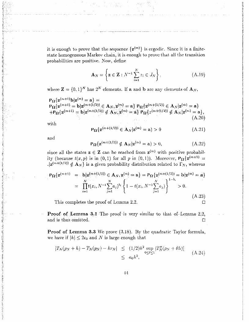
it is enough to prove that the seqlue][1cehomogeneous Markov

pn)DabDlIILIl~S are

it is a finite­transition

AN = {z E Z: (A.19)

where Z {O, 1}N has 2N elements. If a and bare elements of AN,

E ANlz(m) a}ANlz(m)=a},

(A.20)

(A.21)

Pn{z(m+l)blz(m) = a}Pn{z(m+l)= blz(m+(I/2» E

+Pn{z(m+l) 1:

with

andPn{z(m+(1/2» 1:. ANlz(m) a) > 0, (A.22)

since all the states z E Z can be reached from z(m) with positive probabil­ity (because t(x,p) is in (0,1) for all p in (0,1)). Moreover, Pn{z(m+l).lz(m+(1/2» 1:. AN} is a given probability distribution related to r N, whereas

Pn{z(m+l) bl~(m+(1/2» E AN, z(m)::::: a} = Pn{z(m+(1/2»= blz(m) =a}

= gt(x;,N-1t,a;)O, {I -t(x;,N-1t,a j ) ro, > o.

This completes proof of Lemma 2.2.(A.23)

o

Proof of Lemma 3.3we if

prove (3.18). By the qmLari'LtlC LUV·iVi formula,IS

+ <

<+

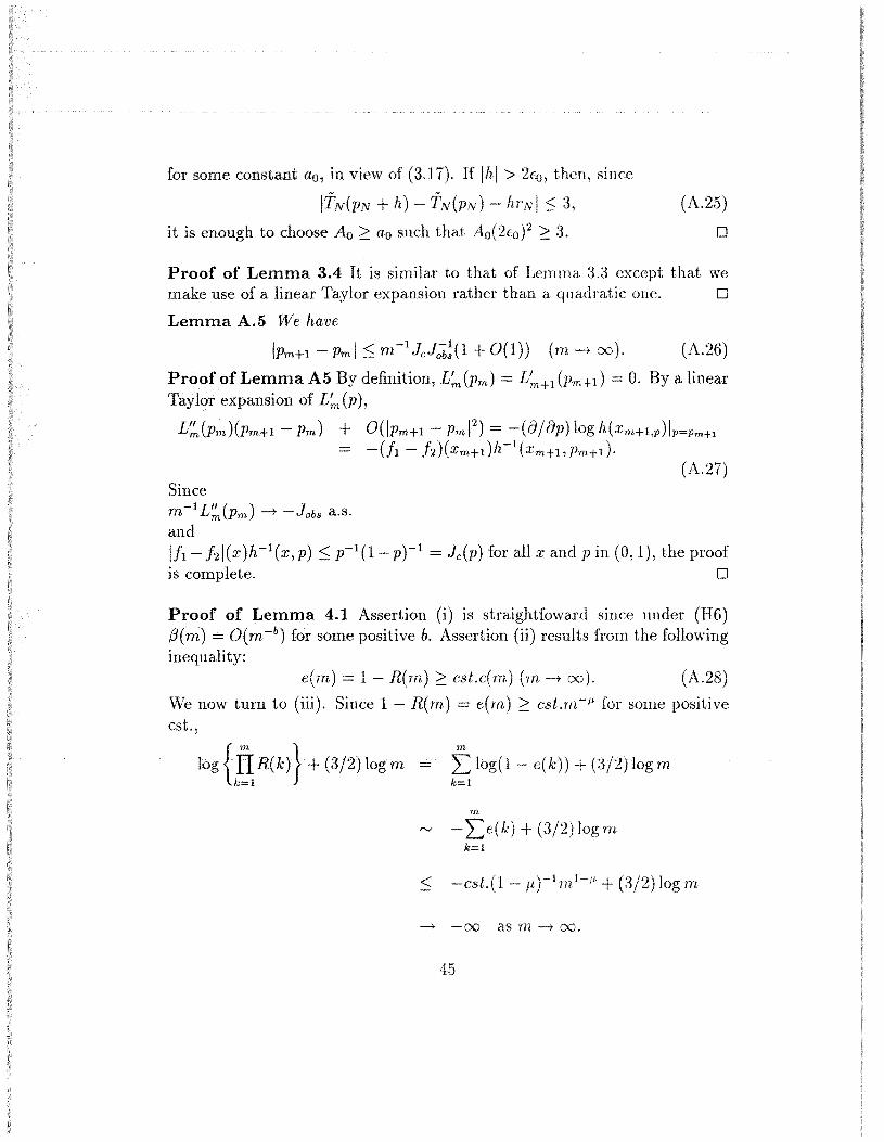
for some constant ao, in of (3.17). If Ihl > 2Eo, then, since

rrN(PN h) - TN(PN) hrNI:::; 3,

it is enough to choose Ao 2': ao such that A o(2co)2 2': 3.

(A.25)

o

Proof of Lemma 3.4 It is similar to that of Lemma :3.3 except that weuse of a linear Taylor expansion rather than a quadratic one. 0

Lemma A.5 We have

(A.26)

Proof of Lemma A5 By definition, L'm (Pm) = L~lH (PmH) O. By a linearTaylor expansion of L'm (p),

L~(Pm)(PmH - Pm) + O(IPmH - Pm1 2) = -(a/ap) log h(XmH,p)IP=Pm+l

-(it - h)(xm+dh-1(xm+I,Pm+d·(A.27)

Sincem-1L~(Pm) -+ -Jobs a.s.andIf1 - hl(x )h-1(x,p) :::; p-1(1- pt1 = Jc(p) for all x and P in (0,1), the proofis complete. 0

Proof of Lemma 4.1 Assertion (i) is straightfoward since under (H6)f3( m) = O(m -b) for some positive b. Assertion (ii) results from the followinginequality:

e(m) = 1 - R(m) 2': cst.c(m) (m -+ (0). (A.28)

We now turn to (iii). Since 1 - R(m) = e(m) 2': cst.m-" for some positivecst.,

log {gR(k)} (3/2) log Tn

m

I: log(1 e(k)) (:3/2)log m1<:=1

m

rv - I:e(k) + (3/2) log m1<:=1

< m

-+ -00 as -+ 00.

proof of 13) is snrnlar. o

IEEE

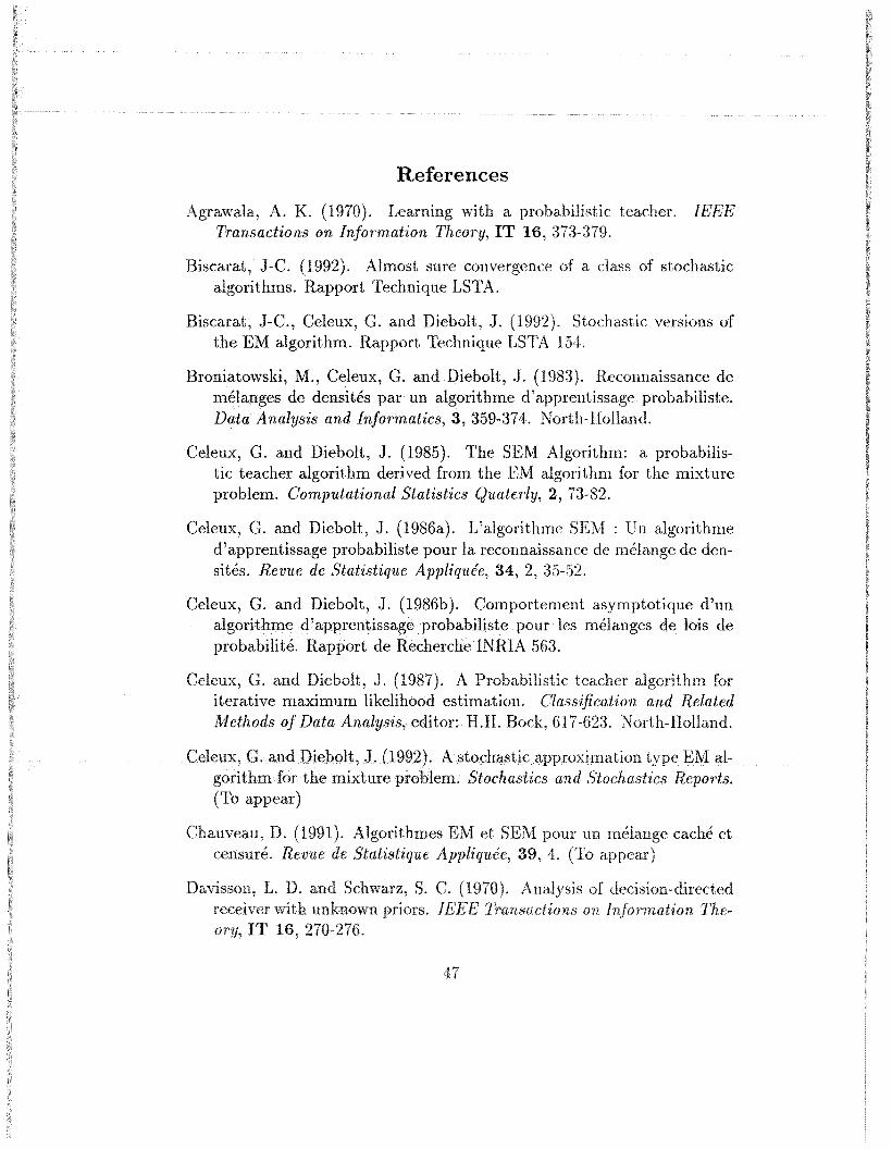
References

Agrawala, A. K. with aTransactions on Information Theory, IT 16, 373-379.

Biscarat, J-C. (1992). Almost sure convergence of a class of stochasticalgorithms. Rapport Technique LSTA.

Biscarat, J-C., Celeux, G. and Diebolt, J. (1992). Stochastic versions ofthe EM algorithm. Rapport Technique LSTA 154.

Broniatowski, M., Celeux, G. and Diebolt, J. (1983). Reconnaissance demelanges de densites par un algorithme d'apprentissage probabiliste.Data Analysis and Informatics, 3,359-374. North-Holland.

Celeux, G. and Diebolt, J. (1985). The SEM Algorithm: a probabilis­tic teacher algorithm derived from the EM algorithm for the mixtureproblem. Computational Statistics Quaterly, 2, 73-82.

Celeux, G. and Diebolt, J. (1986a). L'algorithme SEM : Un algorithmed'apprentissage probabiliste pour la reconnaissance de melange de den­sites. Revue de Statistique Appliquee, 34, 2, 35-52.

Celeux, G. and Diebolt, J. (1986b). Comportement asymptotique d'unalgorithme d'apprentissageprobabiliste pour les melanges lois deprobabilite. Rapport de Recherche INRIA 563.

Celeux, G. and Diebolt, J. (1987). A Probabilistic teacher algorithm foriterative maximum likelihood estimation. Classification and RelatedMethods of Data Analysis, editor: H.H. Bock, 617-623. North-Holland.

pr()l:)l~~m. Stochastics and Stochastics Reports.(To appear)

Chauveau, D. (1991). SEM pour un mE~larl.e;e

cerlsure. Revue de ::>tCJ&tzstzqtte Appliquee, 39,et

Theory ofDavydov, Y. A. (1973). Mixing conditionsProbability and Applications, 18, 312-328.

Dempster, A. P., Laird, N. M. and Rubin, D. B. (1977). Maximum like-lihood from incomplete data via EM algorithm (with discussion).Journal of the Royal Statistical Society, Ser. B 39, 1-38.

Diebolt, J. and Robert, C. P. (1992). Estimation of finite mixture distri­butions through Bayesian sampling. Journal of the Royal StatisticalSociety, Ser. B. (To appear)

Feller, W. (1971) An Introduction to Probability Theory and its Applica­tions, Vol. 2. New York: Wiley.

Kazakos, D. (1977). Recursive estimation of prior probabilities using amixtures. IEEE Transactions on Information Theory, IT 23, 203-211.

Louis, T. (1982). Finding the observed information matrix when using theEM algorithm. Journal of the Royal Statistical Society, Ser. B 44,226-233.

Makov, U. E. and Smith, A. F. (1977). A Quasi-Bayes unsupervised learn­ing procedure for priors. IEEE Transactions on Info'rmation Theory,IT 23. 761-764.

Odell, P. L. and Basu, J. P. (1976). Concerning several methods for esti­mating crop acreages using remote sensing data. Communications inStatistics (AJ, 5, 1091-1114.

Owen, J. R. (1975). A Bayesian sequential procedure for quantal responsein the context of adaptative mental Journal of the AmericanStatistical Association, 70, 351-356.

Redner, R. A. and Walker, H. F. (1984). Mixture derlsltles, ma,xrrnUJmlikelihood and the algorithm. SIA1Y 26, 195-239.

Some probabilisticIT 26, Z~f)-Z~~_

(1976).equations for incomplete data

Statistics Simul. Comput. (B), 5.

Shorack, G. R. and Wellner J. A. (1986) Empirical Processes with Appli-cations to Statistics. New York: ·Wiley.

Tanner, M. A. and "Vong, W. H. (1987). The calculation of posteriordistribution by data augmentation. Journal of the American StatisticalAssociation, 82, 528-550.

plete data .11)1'1'1''1111/

lte:Ctl.lrSliie par.amE~ter estimation::>tlztUj:tic,al Society, Ser. B 46, "".J "-"",11

Titterington, D. M., Smith A.F. and Makov U. (1985). StatisticalAnalysis of Finite Mixture Distributions. New York: vViley. Journal ofthe Royal Statistical Society, Ser. B 46, 257-267.

Wei, G.C.G. and Tanner, M. A. (1990). A Monte-Carlo Implementation ofthe EM algorithm and the poor man's data augmentation algorithms.Journal of the American Statistical Association, 85, 699-704.

\Vindham, M. P. and Cutler, A. (1991). Information ratios for validatingduster analyses. UtahSti.'tte University (Logan).

"Vu, C. F. (1983). On the convergence properties of the EM algorithm.Annals of Statistics, 11, 95-103.