at the molecular scale - arxiv.org
TRANSCRIPT

arX
iv:0
805.
0628
v2 [
cond
-mat
.mes
-hal
l] 1
4 Ju
l 200
8
Green function techniquesin the treatment of quantum transportat the molecular scale
D. A. Ryndyk, R. Gutierrez, B. Song, and G. Cuniberti
Abstract The theoretical investigation of charge (and spin) transport atnanometer length scales requires the use of advanced and powerful tech-niques able to deal with the dynamical properties of the relevant physicalsystems, to explicitly include out-of-equilibrium situations typical for elec-trical/heat transport as well as to take into account interaction effects in asystematic way. Equilibrium Green function techniques and their extensionto non-equilibrium situations via the Keldysh formalism build one of the pil-lars of current state-of-the-art approaches to quantum transport which havebeen implemented in both model Hamiltonian formulations and first-principlemethodologies. In this chapter we offer a tutorial overview of the applicationsof Green functions to deal with some fundamental aspects of charge trans-port at the nanoscale, mainly focusing on applications to model Hamiltonianformulations.
DmitryA. RyndykInstitute for Theoretical Physics, University of Regensburg,D-93040 Regensburg, Germany,e-mail: [email protected]
Rafael GutierrezInstitute for Material Science and Max Bergmann Center of Biomaterials,Dresden University of Technology, D-01062 Dresden, Germany,e-mail: [email protected]
Bo SongInstitute for Material Science and Max Bergmann Center of Biomaterials,Dresden University of Technology, D-01062 Dresden, Germany,e-mail: [email protected]
Gianaurelio CunibertiInstitute for Material Science and Max Bergmann Center of Biomaterials,Dresden University of Technology, D-01062 Dresden, Germany,e-mail: [email protected]
1

2 D. A. Ryndyk, R. Gutierrez, B. Song, and G. Cuniberti
1 Introduction
The natural limitations that are expected to arise by the further miniaturiza-tion attempts of semiconductor-based electronic devices have led in the pasttwo decades to the emergence of the new field of molecular electronics, whereelectronic functions are going to be performed at the single-molecule level,see recent overview in Refs. [1, 2, 3, 4, 5, 6]. The original conception whichlies at the bottom of this fascinating field can be traced back to the paper byAri Aviram and Mark Ratner in 1974 [7], where a single-molecule rectifyingdiode was proposed. Obviously, one of the core issues at stake in molecu-lar electronics is to clarify the question whether single molecules (or morecomplex molecular aggregates) can support an electric current. To achievethis goal, extremely refined experimental techniques are required in order toprobe the response of such a nano-object to external fields. The meanwhileparadigmatic situation is that of a single molecule contacted by two metallicelectrodes between which a bias voltage is applied.
Recent experiments
Enormous progress has been achieved in the experimental realization ofsuch nano-devices, we only mention the development of controllable single-molecule junctions [8]-[22] and scanning tunneling microscopy based tech-niques [23]-[44]. With their help, a plethora of interesting phenomena likerectification [18], negative differential conductance [9, 35], Coulomb block-ade [23, 10, 11, 15, 16, 21], Kondo effect [11, 12], vibrational effects [10, 25, 13,14, 16, 31, 32, 33, 35, 36, 21], and nanoscale memory effects [34, 39, 40, 42, 44],among others, have been demonstrated.
The traditional semiconductor nanoelectronics also remains in front ofmodern research, in particular due to recent experiments with small quantumdots, where cotunneling effects were observed [45, 46, 47], as well as newrectification effects in double quantum dots, interpreted as spin blockade [48,49, 50, 51]. Note, that semiconductor experiments are very well controlled atpresent time, so they play an important role as a benchmark for the theory.
Apart from single molecules, carbon nanotubes have also found extensiveapplications and have been the target of experimental and theoretical studiesover the last years, see Ref. [52] for a very recent review. The expectationsto realize electronics at the molecular scale also reached into the domain ofbio-molecular systems, thus opening new perspectives for the field due to thespecific self-recognition and self-assembling properties of biomolecules. Forinstance, DNA oligomers have been already used as templates in molecularelectronic circuits [53, 54, 55]. Much less clear is, however, if bio-molecules,and more specifically short DNA oligomers could also act as wiring systems.Their electrical response properties are much harder to disclose and there
Green function techniques in the treatment of quantum transport 3
is still much controversy about the factors that determine charge migrationthrough such systems [56, 57, 58, 59, 60, 61, 62, 63, 64].
Theoretical methods
The theoretical treatment of transport at the nanoscale (see introductionin [65, 66, 67, 68, 69, 70]) requires the combined use of different tech-niques which range from minimal model Hamiltonians, passing through semi-empirical methods up to full first-principle methodologies. We mention heresome important contributions, while we have no possibility to cite all relevantpapers.
Model Hamiltonians can in a straightforward way select, out of the manyvariables that can control charge migration those which are thought to bethe most relevant ones for a specific molecule-electrode set-up. They con-tain, however, in a sometimes not well-controlled way, many free parameters;hence, they can point at generic effects, but they must be complementedwith other methodologies able to yield microscopic specific information. Semi-empirical methods can deal with rather large systems due to the use of specialsubsets of electronic states to construct molecular Hamiltonians as well as tothe approximate treatment of interactions, but often have the drawback ofnot being transferable. Ab initio approaches, finally, can deal in a very precisemanner with the electronic and atomic structure of the different constituentsof a molecular junction (metallic electrodes, molecular wire, the interface)but it is not apriori evident that they can also be applied to strong non-equilibrium situations.
From a more formal standpoint, there are roughly two main theoreticalframeworks that can be used to study quantum transport in nanosystems atfinite voltage: generalized master equations (GME) [71, 72] and nonequilib-rium Green function (NGF) techniques [73, 74, 75, 76, 66]. The former alsolead to more simple rate equations in the case where (i) the electrode-systemcoupling can be considered as a weak perturbation, and (ii) off-diagonal el-ements of the reduced density matrix in the eigenstate representation (co-herences) can be neglected due to very short decoherence times. Both ap-proaches, the GME and NGF techniques, can yield formally exact expressionsfor many observables. For non-interacting systems, one can even solve ana-lytically many models. However, once interactions are introduced - and theseare the most interesting cases containing a very rich physics - different ap-proximation schemes have to be introduced to make the problems tractable.
In this chapter, we will review mainly the technique of non-equilibriumGreen functions. This approach is able to deal with a very broad varietyof physical problems related to quantum transport at the molecular scale.It can deal with strong non-equilibrium situations via an extension of theconventional GF formalism to the Schwinger-Keldysh contour [74] and itcan also include interaction effects (electron-electron, electron-vibron, etc)

4 D. A. Ryndyk, R. Gutierrez, B. Song, and G. Cuniberti
in a systematic way (diagrammatic perturbation theory, equation of motiontechniques). Proposed first time for the mesoscopic structures in the earlyseventies by Caroli et al. [77, 78, 79, 80], this approach was formulated in anelegant way by Meir, Wingreen and Jauho [81, 82, 83, 66, 84], who derivedexact expression for nonequilibrium current through an interacting nanosys-tem placed between large noninteracting leads in terms of the nonequilibriumGreen functions of the nanosystem. Still, the problem of calculation of theseGreen functions is not trivial. We consider some possible approaches in thecase of electron-electron and electron-vibron interactions. Moreover, as wewill show later on, it can reproduce results obtained within the master equa-tion approach in the weak coupling limit to the electrodes (Coulomb block-ade), but it can also go beyond this limit and cover intermediate coupling(Kondo effect) and strong coupling (Fabry-Perot) domains. It thus offer thepossibility of dealing with different physical regimes in a unified way.
Now we review briefly some results obtained recently in the main directionsof modern research: general nanoscale quantum transport theory, atomistictransport theory and applications to particular single-molecule systems.
General nanoscale quantum transport theory
On the way to interpretation of modern experiments with single-moleculejunctions and STM spectroscopy of single molecules on surfaces, two maintheoretical problems are to be solved. The first is development of appropriatemodels based on ab initio formulation. The second is effective and scalabletheory of quantum transport through multilevel interacting systems. We firstconsider the last problem, assuming that the model Hamiltonian is known.Quantum transport through noninteracting system can be considered usingthe famous Landauer-Buttiker method [85, 86, 87, 88, 89, 90, 91, 92, 93, 94],which establishes the fundamental relation between the wave functions (scat-tering amplitudes) of a system and its conducting properties. The methodcan be applied to find the current through a noninteracting system or throughan effectively noninteracting system, for example if the mean-field descriptionis valid and the inelastic scattering is not essential. Such type of an electrontransport is called coherent, because there is no phase-breaking and quan-tum interference is preserved during the electron motion across the system. Infact, coherence is initially assumed in many ab initio based transport meth-ods (DFT+NGF, and others), so that the Landauer-Buttiker method is nowroutinely applied to any basic transport calculation through nanosystemsand single molecules. Besides, it is directly applicable in many semiconduc-tor quantum dot systems with weak electron-electron interactions. Due tosimplicity and generality of this method, it is now widely accepted and is inthe base of our understanding of coherent transport.
However, the peculiarity of single-molecule transport is just essential role ofelectron-electron and electron-vibron interactions, so that Landauer-Buttiker

Green function techniques in the treatment of quantum transport 5
method is not enough usually to describe essential physics even qualitatively.During last years many new methods were developed to describe transportat finite voltage, with focus on correlation and inelastic effects, in particularin the cases when Coulomb blockade, Kondo effect and vibronic effects takeplace.
Vibrons (the localized phonons) are very important because moleculesare flexible. The theory of electron-vibron interaction has a long history,but many questions it implies are not answered up to now. While the iso-lated electron-vibron model can be solved exactly by the so-called polaronor Lang-Firsov transformation [95, 96, 97], the coupling to the leads pro-duces a true many-body problem. The inelastic resonant tunneling of singleelectrons through the localized state coupled to phonons was considered inRefs. [98, 99, 100, 101, 102, 103]. There the exact solution in the single-particle approximation was derived, ignoring completely the Fermi sea in theleads. At strong electron-vibron interaction and weak couplings to the leadsthe satellites of the main resonant peak are formed in the spectral function.
The essential progress in calculation of transport properties in the strongelectron-vibron interaction limit has been made with the help of the masterequation approach [104, 105, 106, 107, 108, 109, 110, 111, 112]. This method,however, is valid only in the limit of very weak molecule-to-lead coupling andneglects all spectral effects, which are the most important at finite couplingto the leads.
At strong coupling to the leads and the finite level width the master equa-tion approach can no longer be used, and we apply alternatively the nonequi-librium Green function technique which have been recently developed to treatvibronic effects in a perturbative or self-consistent way in the cases of weakand intermediate electron-vibron interaction [113, 114, 115, 116, 117, 118,119, 120, 121, 122, 123, 124, 125, 126, 127, 128, 129, 130].
The case of intermediate and strong electron-vibron interaction at inter-mediate coupling to the leads is the most interesting, but also the most diffi-cult. The existing approaches are mean-field [131, 132, 133], or start from theexact solution for the isolated system and then treat tunneling as a pertur-bation [134, 135, 136, 137, 138, 139, 140]. The fluctuations beyond mean-fieldapproximations were considered in Refs. [141, 142]
In parallel, the related activity was in the field of single-electron shuttlesand quantum shuttles [143, 144, 145, 146, 147, 148, 149, 150, 151, 152, 153].Finally, based on the Bardeen’s tunneling Hamiltonian method [154, 155, 156,157, 158] and Tersoff-Hamann approach [159, 160], the theory of inelasticelectron tunneling spectroscopy (IETS) was developed [161, 162, 113, 114,115, 116, 163].
The recent review of the electron-vibron problem and its relation to themolecular transport see in Ref. [164].
Coulomb interaction is the other important ingredient of the models,describing single molecules. It is in the origin of such fundamental effects asCoulomb blockade and Kondo efect. The most convenient and simple enough

6 D. A. Ryndyk, R. Gutierrez, B. Song, and G. Cuniberti
is Anderson-Hubbard model, combining the formulations of Anderson impu-rity model [165] and Hubbard many-body model [166, 167, 168]. To analyzesuch strongly correlated system several complementary methods can be used:master equation and perturbation in tunneling, equation-of-motion method,self-consistent Green functions, renormalization group and different numeri-cal methods.
When the coupling to the leads is weak, electron-electron interaction re-sults in Coulomb blockade, the sequential tunneling is described by the mas-ter equation method [169, 170, 171, 172, 173, 174, 175, 176] and small co-tunneling current in the blockaded regime can be calculated by the next-order perturbation theory [177, 178, 179]. This theory was used success-fully to describe electron tunneling via discrete quantum states in quantumdots [180, 181, 182, 183]. Recently there were several attempts to apply masterequation to multi-level models of molecules, in particular describing benzenerings [184, 185, 186].
To describe consistently cotunneling, level broadening and higher-order(in tunneling) processes, more sophisticated methods to calculate the re-duced density matrix were developed, based on the Liouville - von Neumannequation [187, 188, 189, 190, 191, 192, 193, 186] or real-time diagrammatictechnique [194, 195, 196, 197, 198, 199, 200, 201]. Different approaches werereviewed recently in Ref. [202].
The equation-of-motion (EOM) method is one of the basic and powerfulways to find the Green functions of interacting quantum systems. In spite ofits simplicity it gives the appropriate results for strongly correlated nanosys-tems, describing qualitatively and in some cases quantitatively such impor-tant transport phenomena as Coulomb blockade and Kondo effect in quantumdots. The results of the EOM method could be calibrated with other availablecalculations, such as the master equation approach in the case of weak cou-pling to the leads, and the perturbation theory in the case of strong couplingto the leads and weak electron-electron interaction.
In the case of a single site junction with two (spin-up and spin-down) statesand Coulomb interaction between these states (Anderson impurity model),the linear conductance properties have been successfully studied by means ofthe EOM approach in the cases related to Coulomb blockade[203, 204] andthe Kondo effect [205]. Later the same method was applied to some two-sitemodels [206, 207, 208, 209]. Multi-level systems were started to be consideredonly recently [210, 211]. Besides, there are some difficulties in building thelesser GF in the nonequilibrium case (at finite bias voltages) by means of theEOM method [212, 213, 214].
The diagrammatic method was also used to analyze the Anderson impu-rity model. First of all, the perturbation theory can be used to describe weakelectron-electron interaction and even some features of the Kondo effect [215].The family of nonperturbative current-conserving self-consistent approxima-tions for Green functions has a long history and goes back to the Schwingerfunctional derivative technique, Kadanoff-Baym approximations and Hedin

Green function techniques in the treatment of quantum transport 7
equations in the equilibrium many-body theory [216, 217, 218, 219, 220, 221,222, 223]. Recently GW approximation was investigated together with othermethods [224, 225, 226, 227]. It was shown that dynamical correlation effectsand self-consistency can be very important at finite bias.
Finally, we want to mention briefly three important fields of research, thatwe do not consider in the present review: the theory of Kondo effect [228,229, 230, 205, 231, 232, 233, 234], spin-dependent transport [235, 236, 237,238, 239], and time-dependent transport [83, 240, 241, 242, 243].
Atomistic transport theory
Atomistic transport theory utilizes semi-empirical (tight-binding [244, 245])or ab initio based methods. In all cases the microscopic structure is takeninto account with different level of accuracy.
The most popular is the approach combining density-functional theory(DFT) and NGF and known as DFT+NGF [246, 247, 248, 249, 250, 251,252, 253, 254, 255, 256, 257, 258, 259, 260, 261, 262, 263, 264, 265, 266,267, 268]. This method, however is not free from internal problems. Firstof all, it is essentially mean-filed method neglecting strong local correlationsand inelastic scattering. Second, density-functional theory is a ground statetheory and e.g. the transmission calculated using static DFT eigenvalues willdisplay peaks at the Kohn-Sham excitation energies, which in general do notcoincide with the true excitation energies. Extensions to include excited statesas in time-dependent density-functional theory, though very promising [269,270, 271], are not fully developed up to date.
To improve DFT-based models several approaches were suggested, includ-ing inelastic electron-vibron interaction [121, 272, 273, 126, 274, 275, 276,277, 278, 279] or Coulomb interaction beyond mean-field level [280], or basedon the LDA+U approache [281]. The principally different alternative to DFTis to use an initio quantum chemistry based many-body quantum transportapproach [282, 283, 284, 285].
Finally, transport in bio-molecules attracted more attention, in particularelectrical conductance of DNA [286, 287, 288, 289, 290].
Outline
The review is organized as follows. In Sections 2 we will first introducethe Green functions for non-interacting systems, and present few examplesof transport through non-interacting regions. Then we review the masterequation approach and its application to describe Coulomb blockade andvibron-mediated Franck-Condon blockade. In Section 3 the Keldysh NGFtechnique is developed in detail. In equilibrium situations or within the lin-ear response regime, dynamic response and static correlation functions are

8 D. A. Ryndyk, R. Gutierrez, B. Song, and G. Cuniberti
related via the fluctuation-dissipation theorem. Thus, solving Dyson equa-tion for the retarded GF is enough to obtain the correlation functions. Instrong out-of-equilibrium situations, however, dynamic response and corre-lation functions have to be calculated simultaneously and are not relatedby fluctuation-dissipation theorems. The Kadanof-Baym-Keldysh approachyield a compact, powerful formulation to derive Dyson and kinetic equationsfor non-equilibrium systems. In Sec. 4 we present different applications of theGreen function techniques. We show how Coulomb blockade can be describedwithin the Anderson-Hubbard model, once an appropriate truncation of theequation of motion hierarchy is performed (Sec. 4.A). Further, the paradig-matic case of transport through a single electronic level coupled to a localvibrational mode is discussed in detail within the context of the self-consistentBorn approximation. It is shown that already this simple model can displaynon-trivial physics (Sec. 4.B). Finally, the case of an electronic system inter-acting with a bosonic bath is discussed in Sec. 4.C where it is shown thatthe presence of an environment with a continuous spectrum can modified thelow-energy analytical structure of the Green function and lead to dramaticchanges in the electrical response of the system. We point at the relevanceof this situation to discuss transport experiments in short DNA oligomers.We have not addressed the problem of the (equilibrium or non-equilibrium)Kondo effect, since this issue alone would require a chapter on its own dueto the non-perturbative character of the processes leading to the formationof the Kondo resonance.
In view of the broadness of the topic, the authors were forced to do avery subjective selection of the topics to be included in this review as well asof the most relevant literature. We thus apologize for the omission of manyinteresting studies which could not be dealt with in the restricted space atour disposal. We refer the interested reader to the other contributions in thisbook and the cited papers.

Green function techniques in the treatment of quantum transport 9
2 From coherent transport to sequential tunneling(basics)
2.1 Coherent transport: single-particle Green functions
Nano-scale and molecular-scale systems are naturally described by the discrete-level models, for example eigenstates of quantum dots, molecular orbitals, oratomic orbitals. But the leads are very large (infinite) and have a continuousenergy spectrum. To include the lead effects systematically, it is reasonableto start from the discrete-level representation for the whole system. It canbe made by the tight-binding (TB) model, which was proposed to describequantum systems in which the localized electronic states play an essentialrole, it is widely used as an alternative to the plane wave description of elec-trons in solids, and also as a method to calculate the electronic structure ofmolecules in quantum chemistry.
A very effective method to describe scattering and transport is the Greenfunction (GF) method. In the case of non-interacting systems and coherenttransport single-particle GFs are used. In this section we consider the matrixGreen function method for coherent transport through discrete-level systems.
(i) Matrix (tight-binding) Hamiltonian
The main idea of the method is to represent the wave function of a particleas a linear combination of some known localized states ψα(r, σ), where αdenote the set of quantum numbers, and σ is the spin index (for example,atomic orbitals, in this particular case the method is called LCAO – linearcombination of atomic orbitals)
ψ(ξ) =∑
α
cαψα(ξ), (1)
here and below we use ξ ≡ (r, σ) to denote both spatial coordinates and spin.Using the Dirac notations |α〉 ≡ ψα(ξ) and assuming that ψα(ξ) are or-
thonormal functions 〈α|β〉 = δαβ we can write the single-particle matrix(tight-binding) Hamiltonian in the Hilbert space formed by ψα(ξ)
H =∑
α
(ǫα + eϕα)|α〉〈α| +∑
αβ
tαβ |α〉〈β|, (2)
the first term in this Hamiltonian describes the states with energies ǫα, ϕα
is the electrical potential, the second term should be included if the states|α〉 are not eigenstates of the Hamiltonoian. In the TB model tαβ is thehopping matrix element between states |α〉 and |β〉, which is nonzero, as arule, for nearest neighbor cites. The two-particle interaction is described by

10 D. A. Ryndyk, R. Gutierrez, B. Song, and G. Cuniberti
the HamiltonianH =
∑
αβ,δγ
Vαβ,δγ |α〉|β〉〈δ|〈γ|, (3)
in the two-particle Hilbert space, and so on.The energies and hopping matrix elements in this Hamiltomian can be
calculated, if the single-particle real-space Hamiltomian h(ξ) is known:
ǫαδαβ + tαβ =
∫
ψ∗α(ξ)h(ξ)ψβ(ξ)dξ. (4)
This approach was developed originally as an approximate method, if thewave functions of isolated atoms are taken as a basis wave functions ψα(ξ),but also can be formulated exactly with the help of Wannier functions. Onlyin the last case the expansion (1) and the Hamiltonian (2) are exact, butsome extension to the arbitrary basis functions is possible. In principle, theTB model is reasonable only when local states can be orthogonalized. Themethod is useful to calculate the conductance of complex quantum systemsin combination with ab initio methods. It is particular important to describesmall molecules, when the atomic orbitals form the basis.
In the mathematical sense, the TB model is a discrete (grid) version ofthe continuous Schrodinger equation, thus it is routinely used in numericalcalculations.
To solve the single-particle problem it is convenient to introduce a new rep-resentation, where the coefficients cα in the expansion (1) are the componentsof a vector wave function (we assume here that all states α are numeratedby integers)
Ψ =
c1c2...cN
, (5)
and the eigenstates Ψλ are to be found from the matrix Schrodinger equation
HΨλ = EλΨλ, (6)
with the matrix elements of the single-particle Hamiltonian
Hαβ =
ǫα + eϕα, α = β,tαβ , α 6= β.
(7)
Now let us consider some typical systems, for which the matrix method isappropriate starting point. The simplest example is a single quantum dot, thebasis is formed by the eigenstates, the corresponding Hamiltonian is diagonal

Green function techniques in the treatment of quantum transport 11
1ε 2ε 1Nε − Nε
t t tFig. 1 A finite linear chain of single-level sites.
H =
ǫ1 0 0 · · · 00 ǫ2 0 · · · 0...
. . .. . .
. . ....
0 · · · 0 ǫN−1 00 · · · 0 0 ǫN
. (8)
The next typical example is a linear chain of single-state sites with onlynearest-neighbor couplings (Fig. 1)
H =
ǫ1 t 0 · · · 0t ǫ2 t · · · 0...
. . .. . .
. . ....
0 · · · t ǫN−1 t0 · · · 0 t ǫN
. (9)
The method is applied as well to consider the semi-infinite leads. Althoughthe matrices are formally infinitely-dimensional in this case, we shall showbelow, that the problem is reduced to the finite-dimensional problem for thequantum system of interest, and the semi-infinite leads can be integrated out.
Finally, in the second quantized form the tight-binding Hamiltonian is
H =∑
α
(ǫα + eϕα) c†αcα +∑
α6=β
tαβc†αcβ. (10)
(ii) Matrix Green functions and contact self-energies
The solution of single-particle quantum problems, formulated with the helpof a matrix Hamiltonian, is possible along the usual line of finding thewave-functions on a lattice, solving the Schrodinger equation (6). The othermethod, namely matrix Green functions, considered in this section, was foundto be more convenient for transport calculations, especially when interactionsare included.
The retarded single-particle matrix Green function GR(ǫ) is determinedby the equation
[(ǫ+ iη)I − H]GR = I, (11)

12 D. A. Ryndyk, R. Gutierrez, B. Song, and G. Cuniberti
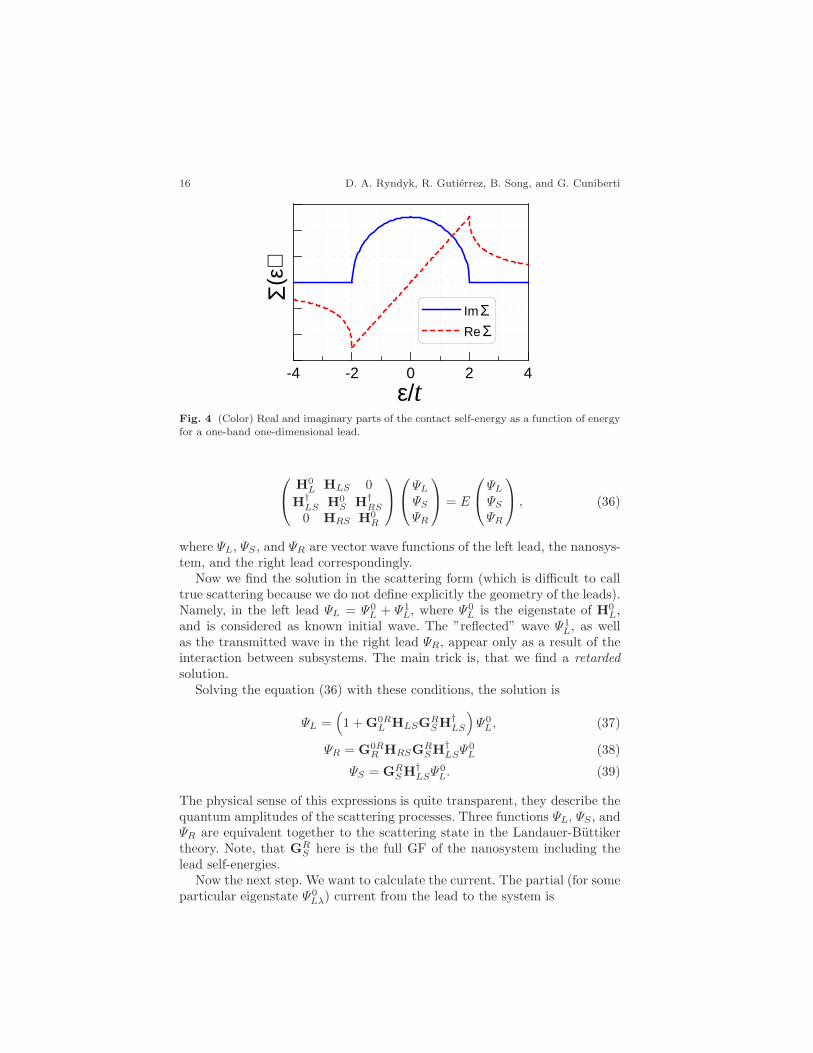
System
L R
0HL0HR0HS
HLS HRS
Fig. 2 A quantum system coupled to the left and right leads.
where η is an infinitesimally small positive number η = 0+.For an isolated noninteracting system the Green function is simply ob-
tained after the matrix inversion
GR = [(ǫ+ iη)I − H]−1. (12)
Let us consider the trivial example of a two-level system with the Hamiltonian
H =
(
ǫ1 tt ǫ2
)
. (13)
The retarded GF is easy found to be (ǫ = ǫ+ iη)
GR(ǫ) =1
(ǫ− ǫ1)(ǫ− ǫ2) + t2
(
ǫ− ǫ2 tt ǫ− ǫ1
)
. (14)
Now let us consider the case, when the system of interest is coupled totwo contacts (Fig. 2). We assume here that the contacts are also described bythe tight-binding model and by the matrix GFs. Actually, the semi-infinitecontacts should be described by the matrix of infinite dimension. We shallconsider the semi-infinite contacts in the next section.
Let us present the full Hamiltonian of the considered system in a followingblock form
H =
H0L HLS 0
H†LS H0S H†RS
0 HRS H0R
, (15)
where H0L, H0
S , and H0R are Hamiltonians of the left lead, the system, and
the right lead separately. And the off-diagonal terms describe system-to-leadcoupling. The Hamiltonian should be hermitian, so that
HSL = H†LS , HSR = H†RS . (16)
The Eq. (11) can be written as

Green function techniques in the treatment of quantum transport 13
E− H0L −HLS 0
−H†LS E− H0S −H†RS
0 −HRS E− H0R
GL GLS 0GSL GS GSR
0 GRS GR
= I, (17)
where we introduce the matrix E = (ǫ+ iη)I, and represent the matrix Greenfunction in a convenient form, the notation of retarded function is omitted inintermediate formulas. Now our first goal is to find the system Green functionGS which defines all quantities of interest. From the matrix equation (17)
(
E− H0L
)
GLS − HLSGS = 0, (18)
−H†LSGLS +(
E − H0S
)
GS − H†RSGRS = I, (19)
−HRSGS +(
E− H0R
)
GRS = 0. (20)
From the first and the third equations one has
GLS =(
E − H0L
)−1HLSGS , (21)
GRS =(
E− H0R
)−1HRSGS , (22)
and substituting it into the second equation we arrive at the equation
(
E− H0S − Σ
)
GS = I, (23)
where we introduce the contact self-energy (which should be also called re-tarded, we omit the index in this chapter)
Σ = H†LS
(
E − H0L
)−1HLS + H†RS
(
E− H0R
)−1HRS . (24)
Finally, we found, that the retarded GF of a nanosystem coupled to theleads is determined by the expression
GRS (ǫ) =
[
(ǫ+ iη)I − H0S − Σ
]−1, (25)
the effects of the leads are included through the self-energy.Here we should stress the important property of the self-energy (24), it is
determined only by the coupling Hamiltonians and the retarded GFs of the
isolated leads G0Ri =
(
E− H0R
)−1(i = L,R)
Σi = H†iS(
E − H0i
)−1HiS = H†iSG0R
i HiS , (26)
it means, that the contact self-energy is independent of the state of thenanosystem itself and describes completely the influence of the leads. Laterwe shall see that this property conserves also for interacting system, if theleads are noninteracting.
Finally, we should note, that the Green functions considered in this section,are single-particle GFs, and can be used only for noninteracting systems.

14 D. A. Ryndyk, R. Gutierrez, B. Song, and G. Cuniberti
0ε 0ε
t t
System
Fig. 3 A quantum system coupled to a semi-infinite 1D lead.
(iii) Semi-infinite leads
Let us consider now a nanosystem coupled to a semi-infinite lead (Fig. 3).The direct matrix inversion can not be performed in this case. The spectrumof a semi-infinite system is continuous. We should transform the expression(26) into some other form.
To proceed, we use the relation between the Green function and the eigen-functions Ψλ of a system, which are solutions of the Schrodinger equation (6).Let us define Ψλ(α) ≡ cλ in the eigenstate |λ〉 in the sense of definition (5),then
GRαβ(ǫ) =
∑
λ
Ψλ(α)Ψ∗λ(β)
ǫ+ iη − Eλ, (27)
where α is the TB state (site) index, λ denotes the eigenstate, Eλ is the energyof the eigenstate. The summation in this formula can be easy replaced by theintegration in the case of a continuous spectrum. It is important to notice,that the eigenfunctions Ψλ(α) should be calculated for the separately takensemi-infinite lead, because the Green function of isolated lead is substitutedinto the contact self-energy.
For example, for the semi-infinite 1D chain of single-state sites (n,m =1, 2, ...)
GRnm(ǫ) =
∫ π
−π
dk
2π
Ψk(n)Ψ∗k (m)
ǫ+ iη − Ek, (28)
with the eigenfunctions Ψk(n) =√
2 sin kn, Ek = ǫ0 + 2t cos k.Let us consider a simple situation, when the nanosystem is coupled only to
the end site of the 1D lead (Fig. 3). From (26) we obtain the matrix elementsof the self-energy
Σαβ = V ∗1αV1βG0R11 , (29)
where the matrix element V1α describes the coupling between the end site ofthe lead (n = m = 1) and the state |α〉 of the nanosystem.
Green function techniques in the treatment of quantum transport 15
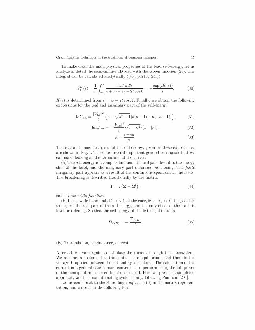
To make clear the main physical properties of the lead self-energy, let usanalyze in detail the semi-infinite 1D lead with the Green function (28). Theintegral can be calculated analytically ([70], p. 213, [244])
GR11(ǫ) =
1
π
∫ π
−π
sin2 kdk
ǫ+ iη − ǫ0 − 2t cosk= −exp(iK(ǫ))
t, (30)
K(ǫ) is determined from ǫ = ǫ0 + 2t cosK. Finally, we obtain the followingexpressions for the real and imaginary part of the self-energy
ReΣαα =|V1α|2t
(
κ−√
κ2 − 1 [θ(κ− 1) − θ(−κ− 1)])
, (31)
ImΣαα = −|V1α|2t
√
1 − κ2θ(1 − |κ|), (32)
κ =ǫ− ǫ0
2t. (33)
The real and imaginary parts of the self-energy, given by these expressions,are shown in Fig. 4. There are several important general conclusion that wecan make looking at the formulas and the curves.
(a) The self-energy is a complex function, the real part describes the energyshift of the level, and the imaginary part describes broadening. The finiteimaginary part appears as a result of the continuous spectrum in the leads.The broadening is described traditionally by the matrix
Γ = i(
Σ− Σ†)
, (34)
called level-width function.(b) In the wide-band limit (t→ ∞), at the energies ǫ−ǫ0 ≪ t, it is possible
to neglect the real part of the self-energy, and the only effect of the leads islevel broadening. So that the self-energy of the left (right) lead is
ΣL(R) = −iΓL(R)
2. (35)
(iv) Transmission, conductance, current
After all, we want again to calculate the current through the nanosystem.We assume, as before, that the contacts are equilibrium, and there is thevoltage V applied between the left and right contacts. The calculation of thecurrent in a general case is more convenient to perform using the full powerof the nonequilibrium Green function method. Here we present a simplifiedapproach, valid for noninteracting systems only, following Paulsson [291].
Let us come back to the Schrodinger equation (6) in the matrix represen-tation, and write it in the following form
16 D. A. Ryndyk, R. Gutierrez, B. Song, and G. Cuniberti
-4 -2 0 2 4
ε/t
Σ (ε)
Im ΣRe Σ
Fig. 4 (Color) Real and imaginary parts of the contact self-energy as a function of energyfor a one-band one-dimensional lead.
H0L HLS 0
H†LS H0S H†RS
0 HRS H0R
ΨL
ΨS
ΨR
= E
ΨL
ΨS
ΨR
, (36)
where ΨL, ΨS , and ΨR are vector wave functions of the left lead, the nanosys-tem, and the right lead correspondingly.
Now we find the solution in the scattering form (which is difficult to calltrue scattering because we do not define explicitly the geometry of the leads).Namely, in the left lead ΨL = Ψ0
L + Ψ1L, where Ψ0
L is the eigenstate of H0L,
and is considered as known initial wave. The ”reflected” wave Ψ1L, as well
as the transmitted wave in the right lead ΨR, appear only as a result of theinteraction between subsystems. The main trick is, that we find a retardedsolution.
Solving the equation (36) with these conditions, the solution is
ΨL =(
1 + G0RL HLSGR
S H†LS
)
Ψ0L, (37)
ΨR = G0RR HRSGR
S H†LSΨ0L (38)
ΨS = GRS H†LSΨ
0L. (39)
The physical sense of this expressions is quite transparent, they describe thequantum amplitudes of the scattering processes. Three functions ΨL, ΨS , andΨR are equivalent together to the scattering state in the Landauer-Buttikertheory. Note, that GR
S here is the full GF of the nanosystem including thelead self-energies.
Now the next step. We want to calculate the current. The partial (for someparticular eigenstate Ψ0
Lλ) current from the lead to the system is

Green function techniques in the treatment of quantum transport 17
ji=L,R =ie
h
(
Ψ †i HiSΨS − Ψ †SH†iSΨi
)
. (40)
To calculate the total current we should substitute the expressions forthe wave functions (37)-(39), and summarize all contributions [291]. As aresult the Landauer formula is obtained. We present the calculation for thetransmission function. First, after substitution of the wave functions we havefor the partial current going through the system
jλ = jL = −jR = − ie
h
(
Ψ †RHRSΨS − Ψ †SH†RSΨR
)
=
− ie
h
(
Ψ0†L HLSGA
S H†RS
(
G0†R − G0
R
)
HRSGRS H†LSΨ
0L
)
=
e
h
(
Ψ0†L HLSGA
S ΓRGRS H†LSΨ
0L
)
. (41)
The full current of all possible left eigenstates is given by
I =∑
λ
jλ =∑
λ
e
h
(
Ψ0†LλHLSGA
S ΓRGRS H†LSΨ
0Lλ
)
fL(Eλ), (42)
the distribution function fL(Eλ) describes the population of the left states,the distribution function of the right lead is absent here, because we consideronly the current from the left to the right.
The same current is given by the Landauer formula through the transmis-sion function T (E)
I =e
h
∫ ∞
−∞
T (E)fL(E)dE. (43)
If one compares these two expressions for the current, the transmissionfunction at some energy is obtained as
T (E) = 2π∑
λ
δ(E − Eλ)(
Ψ0†LλHLSGA
S ΓRGRS H†LSΨ
0Lλ
)
= 2π∑
λ
∑
δ
δ(E − Eλ)(
Ψ0†LλHLSΨδ
)(
Ψ †δ GAS ΓRGR
S H†LSΨ0Lλ
)
=∑
δ
(
Ψ †δ GAS ΓRGR
S H†LS
(
2π∑
λ
δ(E − Eλ)Ψ0LλΨ
0†Lλ
)
HLSΨδ
)
= Tr(
ΓLGAS ΓRGR
S
)
. (44)
To evaluate the sum in brackets we used the eigenfunction expansion (27) forthe left contact.
We obtained the new representation for the transmission formula, whichis very convenient for numerical calculations
T = Tr(
tt†)
= Tr(
ΓLGAΓRGR)
. (45)

18 D. A. Ryndyk, R. Gutierrez, B. Song, and G. Cuniberti
Finally, one important remark, at finite voltage the diagonal energies inthe Hamiltonians H0
L, H0S , and H0
R are shifted ǫα → ǫα +eϕα. Consequently,the energy dependencies of the self-energies defined by (26) are also changedand the lead self-energies are voltage dependent. However, it is convenientto define the self-energies using the Hamiltonians at zero voltage, in thatcase the voltage dependence should be explicitly shown in the transmissionformula
T (E) = Tr[
ΓL(E − eϕL)GR(ǫ)ΓR(E − eϕR)GA(ǫ)]
, (46)
where ϕR and ϕL are electrical potentials of the right and left leads.With known transmission function, the current I at finite voltage V can
be calculated by the usual Landauer-Butiker formulas (without spin degen-eration, otherwise it should be multiplied additionally by 2)
I(V ) =e
h
∫ ∞
−∞
T (E) [fL(E) − fR(E)] dE, (47)
where the equilibrium distribution functions of the contacts should be writtenwith corresponding chemical potentials µi, and electrical potentials ϕi
fL(E) =1
exp(
E−µL−eϕL
T
)
+ 1, fR(E) =
1
exp(
E−µR−eϕR
T
)
+ 1. (48)
The zero-voltage conductance G is
G =dI
dV
∣
∣
∣
∣
V =0
= −e2
h
∫ ∞
−∞
T (E)∂f0(E)
∂EdE, (49)
where f0(E) is the equilibriumfermi-function
f0(E) =1
exp(
E−µT
)
+ 1. (50)

Green function techniques in the treatment of quantum transport 19
2.2 Interacting nanosystems and master equation
method
The single-particle matrix Green function methods, considered in the previ-ous section, can be applied only in the case of noninteracting electrons andwithout inelastic scattering. In the case of interacting systems, the other ap-proach, known as the method of tunneling (or transfer) Hamiltonian (TH),plays an important role, and is widely used to describe tunneling in supercon-ductors, in ferromagnets, effects in small tunnel junctions such as Coulombblockade (CB), etc. The main advantage of this method is that it is easelycombined with powerful methods of many-body theory. Besides, it is veryconvenient even for noninteracting electrons, when the coupling between sub-systems is weak, and the tunneling process can be described by rather simplematrix elements.
2.2.1 Tunneling and master equation
(i) Tunneling (transfer) Hamiltonian
The main idea is to represent the Hamiltonian of the system (we considerfirst a single contact between two subsystems) as a sum of three parts: ”left”HL, ”right” HR, and ”tunneling” HT
H = HL + HR + HT , (51)
HL and HR determine ”left” |Lk〉 and ”right” |Rq〉 states
HLψk(ξ) = Ekψk(ξ), (52)
HRψq(ξ) = Eqψq(ξ), (53)
below in this lecture we use the index k for left states and the index q for rightstates. HT determines ”transfer” between these states and is defined throughmatrix elements Vkq = 〈Lk|HT |Rq〉. With these definitions the single-particletunneling Hamiltonian is
H =∑
k∈L
Ek|k〉〈k| +∑
q∈R
Eq|q〉〈q| +∑
kq
[
Vqk|q〉〈k| + V ∗qk|k〉〈q|]
. (54)
The method of the tunneling Hamiltonian was introduced by Bardeen[154], developed by Harrison [155], and formulated in most familiar secondquantized form by Cohen, Falicov, and Phillips [156]. In spite of many verysuccessful applications of the TH method, it was many times criticized for it’sphenomenological character and incompleteness, beginning from the work ofPrange [157]. However, in the same work Prange showed that the tunneling

20 D. A. Ryndyk, R. Gutierrez, B. Song, and G. Cuniberti
Hamiltonian is well defined in the sense of the perturbation theory. Thesedevelopments and discussions were summarized by Duke [158]. Note, thatthe formulation equivalent to the method of the tunneling Hamiltonian canbe derived exactly from the tight-binding approach.
Indeed, the tight-binding model assumes that the left and right states canbe clearly separated, also when they are orthogonal. The difference with thecontinuous case is, that we restrict the Hilbert space introducing the tight-binding model, so that the solution is not exact in the sense of the continuousSchrodinger equation. But, in fact, we only consider physically relevant states,neglecting high-energy states not participating in transport.
Compare the tunneling Hamiltonian (54) and the tight-binding Hamilto-nian (2), divided into left and right parts
H =∑
αβ∈L
ǫαβ |α〉〈β|+∑
δγ∈R
ǫδγ |δ〉〈γ|+∑
α∈L, δ∈R
[
Vδα|δ〉〈α|+V ∗δα|α〉〈δ|]
. (55)
The first two terms are the Hamiltonians of the left and right parts, thethird term describes the left-right (tunneling) coupling. The equivalent matrixrepresentation of this Hamiltonian is
H =
(
H0L HLR
H†LR H0R
)
. (56)
The Hamiltonians (54) and (55) are essentially the same, only the first oneis written in the eigenstate basis |k〉, |q〉, while the second in the tight-bindingbasis |α〉, |β〉 of the left lead and |δ〉, |γ〉 of the right lead. Now we want totransform the TB Hamiltonian (55) into the eigenstate representation.
Canonical transformations from the tight-binding (atomic orbitals) repre-sentation to the eigenstate (molecular orbitals) representation play an im-portant role, and we consider it in detail. Assume, that we find two unitarymatrices SL and SR, such that the Hamiltonians of the left part H0
L and ofthe right part H0
R can be diagonalized by the canonical transformations
H0L = S−1
L H0LSL, (57)
H0R = S−1
R H0RSR. (58)
The left and right eigenstates can be written as
|k〉 =∑
α
SLkα|α〉, (59)
|q〉 =∑
δ
SRqδ|δ〉, (60)
and the first two free-particle terms of the Hamiltonian (54) are reproduced.The tunneling terms are transformed as

Green function techniques in the treatment of quantum transport 21
HLR = S−1L HLRSR, (61)
H†LR = S−1R H†LRSL, (62)
or explicitly∑
α∈L, δ∈R
Vδα|δ〉〈α| =∑
kq
Vqk|q〉〈k|, (63)
whereVqk =
∑
α∈L, δ∈R
VδαSLαkSRδq. (64)
The last expression solve the problem of transformation of the tight-bindingmatrix elements into tunneling matrix elements.
For applications the tunneling Hamiltonian (54) should be formulated inthe second quantized form. We introduce creation and annihilation Schrodingeroperators c†Lk, cLk, c†Rq, cRq. Using the usual rules we obtain
H = HL
(
c†k; ck
)
+ HR
(
c†q; cq)
+ HT
(
c†k; ck; c†q; cq
)
, (65)
H =∑
k
(ǫk + eϕL(t))c†kck +∑
q
(ǫq + eϕR(t))c†qcq +∑
kq
[
Vqkc†qck + V ∗qkc
†kcq
]
.
(66)It is assumed that left ck and right cq operators describe independent
states and are anticommutative. For nonorthogonal states of the Hamilto-nian Hl + HR it is not exactly so. But if we consider HL and HR as twoindependent Hamiltonians with independent Hilbert spaces we resolve thisproblem. Thus we again should consider (66) not as a true Hamiltonian, butas the formal expression describing the current between left and right states.In the weak coupling case the small corrections to the commutation relationsare of the order of |Vqk| and can be neglected. If the tight-binding formulationis possible, (66) is exact within the framework of this formulation. In generalthe method of tunneling Hamiltonian can be considered as a phenomeno-logical microscopic approach, which was proved to give reasonable results inmany cases, e.g. in description of tunneling between superconductors andJosephson effect.
(ii) Tunneling current
The current from the state k into the state q is given by the golden rule
Jk→q = eΓqk =2πe
h|Vqk|2fL(k) (1 − fR(q)) δ(Ek − Eq), (67)
22 D. A. Ryndyk, R. Gutierrez, B. Song, and G. Cuniberti
the probability (1 − fR(Eq)) that the right state is unoccupied should beincluded, it is different from the scattering approach because left and rightstates are two independent states!
Then we write the total current as the sum of all partial currents fromleft states to right states and vice versa (note that the terms fL(k)fR(q) arecancelled)
J =2πe
h
∑
kq
|Vqk|2 [f(k) − f(q)] δ(Eq − Ek). (68)
For tunneling between two equilibrium leads distribution functions aresimply Fermi-Dirac functions (48) and current can be finally written in thewell known form (To do this one should multiply the integrand on 1 =
∫
δ(E−Eq)dE.)
J =e
h
∫ ∞
−∞
T (E, V ) [fL(E) − fR(E)] dE, (69)
with
T (E, V ) = (2π)2∑
qk
|Vkq |2δ(E − Ek − eϕL)δ(E − Eq − eϕR). (70)
This expression is equivalent to the Landauer formula (47), but the trans-mission function is related now to the tunneling matrix element.
Now let us calculate the tunneling current as the time derivative of thenumber of particles operator in the left lead NL =
∑
k c†kck. Current from
the left to right contact is
J(t) = −e⟨(
dNL
dt
)⟩
S
= − ieh
⟨
[
HT , NL
]
−
⟩
S
, (71)
where 〈...〉S is the average over time-dependent Schrodinger state. NL com-mute with both left and right Hamiltonians, but not with the tunnelingHamiltonian
[
HT , NL
]
−=∑
k′
∑
kq
[(
Vqkc†qck + V ∗qkcqc
†k
)
c†k′ck′
]
−, (72)
using commutation relations
ckc†k′ck′ − c†k′ck′ck = ckc
†k′ck′ + c†k′ckck′ = (ckc
†k′ + δkk′ − ckc
†k′)ck′ = δkk′ck,
we obtain
J(t) =ie
h
∑
kq
[
Vqk
⟨
c†qck⟩
S− V ∗qk
⟨
c†kcq
⟩
S
]
. (73)
Now we switch to the Heisenberg picture, and average over initial time-independent equilibrium state

Green function techniques in the treatment of quantum transport 23
⟨
O(t)⟩
= Sp(
ρeqO(t))
, ρeq =e−Heq/T
Sp(
e−Heq/T) . (74)
One obtains
J(t) =ie
h
∑
kq
[
Vqk
⟨
c†q(t)ck(t)⟩
− V ∗qk
⟨
c†k(t)cq(t)⟩]
. (75)
It can be finally written as
J(t) =2e
hIm
∑
kq
Vqkρkq(t)
=2e
hRe
∑
kq
VqkG<kq(t, t)
.
We define ”left-right” density matrix or more generally lesser Green func-tion
G<kq(t1, t2) = i
⟨
c†q(t2)ck(t1)⟩
.
Later we show that these expressions for the tunneling current give thesame answer as was obtained above by the golden rule in the case of nonin-teracting leads.
(iii) Sequential tunneling and the master equation
Let us come back to our favorite problem – transport through a quantum sys-tem. There is one case (called sequential tunneling), when the simple formulasdiscussed above can be applied even in the case of resonant tunneling
Assume that a noninteracting nanosystem is coupled weakly to a thermalbath (in addition to the leads). The effect of the thermal bath is to breakphase coherence of the electron inside the system during some time τph,called decoherence or phase-breaking time. τph is an important time-scale inthe theory, it should be compared with the so-called ”tunneling time” – thecharacteristic time for the electron to go from the nanosystem to the lead,which can be estimated as an inverse level-width function Γ−1. So that thecriteria of sequential tunneling is
Γτph ≪ 1. (76)
The finite decoherence time is due to some inelastic scattering mechanisminside the system, but typically this time is shorter than the energy relaxationtime τǫ, and the distribution function of electrons inside the system can benonequilibrium (if the finite voltage is applied), this transport regime is wellknown in semiconductor superlattices and quantum-cascade structures.
In the sequential tunneling regime the tunneling events between the leftlead and the nanosystem and between the left lead and the nanosystem areindependent and the current from the left (right) lead to the nanosystem

24 D. A. Ryndyk, R. Gutierrez, B. Song, and G. Cuniberti
is given by the golden rule expression (68). Let us modify it to the case oftunneling from the lead to a single level |α〉 of a quantum system
J =2πe
h
∑
k
|Vαk|2 [f(k) − Pα] δ(Eα − Ek), (77)
where we introduce the probability Pα to find the electron in the state |α〉with the energy Eα.
(iv) Rate equations for noninteracting systems
Rate equation method is a simple approach base on the balance of incomingand outgoing currents. Assuming that the contacts are equilibrium we obtainfor the left and right currents
Ji=L(R) = eΓiα
[
f0i (Eα) − Pα
]
, (78)
where
Γiα =2π
h
∑
k
|Vαk|2δ(Eα − Ek). (79)
In the stationary state J = JL = −JR, and from this condition the levelpopulation Pα is found to be
Pα =ΓLαf
0L(Eα) + ΓRαf
0R(Eα)
ΓLα + ΓRα, (80)
with the current
J = eΓLαΓRα
ΓLα + ΓRα
(
f0L(Eα) − f0
R(Eα))
. (81)
It is interesting to note that this expression is exactly the same, as one canobtain for the resonant tunneling through a single level without any scatter-ing. It should be not forgotten, however, that we did not take into accountadditional level broadening due to scattering.
(v) Master equation for interacting systems
Now let us formulate briefly a more general approach to transport through in-teracting nanosystems weakly coupled to the leads in the sequential tunnelingregime, namely the master equation method. Assume, that the system canbe in several states |λ〉, which are the eigenstates of an isolated system andintroduce the distribution function Pλ – the probability to find the systemin the state |λ〉. Note, that these states are many-particle states, for example

Green function techniques in the treatment of quantum transport 25
for a two-level quantum dot the possible states are |λ〉 = |00〉, |10〉, 01|〉, and|11〉. The first state is empty dot, the second and the third with one electron,and the last one is the double occupied state. The other non-electronic de-grees of freedom can be introduce on the same ground in this approach. Theonly restriction is that some full set of eigenstates should be used
∑
λ
Pλ = 1. (82)
The next step is to treat tunneling as a perturbation. Following this idea,the transition rates Γ λλ′
from the state λ′ to the state λ are calculated usingthe Fermi golden rule
Γ fi =2π
h
∣
∣
∣
⟨
f |HT |i⟩∣
∣
∣
2
δ(Ef − Ei). (83)
Then, the kinetic (master) equation can be written as
dPλ
dt=∑
λ′
Γ λλ′
Pλ′ −∑
λ′
Γ λ′λPλ, (84)
where the first term describes tunneling transition into the state |λ〉, and thesecond term – tunneling transition out of the state |λ〉.
In the stationary case the probabilities are determined from
∑
λ′
Γ λλ′
Pλ′ =∑
λ′
Γ λ′λPλ. (85)
For noninteracting electrons the transition rates are determined by thesingle-electron tunneling rates, and are nonzero only for the transitions be-tween the states with the number of electrons different by one. For example,transition from the state |λ′〉 with empty electron level α into the state |λ〉with filled state α is described by
Γnα=1 nα=0 = ΓLαf0L(Eα) + ΓRαf
0R(Eα), (86)
where ΓLα and ΓRα are left and right level-width functions (79).For interacting electrons the calculation is a little bit more complicated.
One should establish the relation between many-particle eigenstates of thesystem and single-particle tunneling. To do this, let us note, that the states|f〉 and |i〉 in the golden rule formula (83) are actually the states of the wholesystem, including the leads. We denote the initial and final states as
|i〉 = |ki, λ′〉 = |ki〉|λ′〉, (87)
|f〉 = |kf , λ〉 = |kf 〉|λ〉, (88)

26 D. A. Ryndyk, R. Gutierrez, B. Song, and G. Cuniberti
where k is the occupation of the single-particle states in the lead. The pa-rameterization is possible, because we apply the perturbation theory, andisolated lead and nanosystem are independent.
The important point is, that the leads are actually in the equilibriummixed state, the single electron states are populated with probabilities, givenby the Fermi-Dirac distribution function. Taking into account all possiblesingle-electron tunneling processes, we obtain the incoming tunneling rate
Γ λλ′
in =2π
h
∑
ikσ
f0i (Eikσ)
∣
∣
⟨
ik, λ∣
∣HT
∣
∣ ik, λ′⟩∣
∣
2δ(Eλ′ + Eikσ − Eλ), (89)
where we use the short-hand notations: |ik, λ′〉 is the state with occupiedk-state in the i−th lead, while |ik, λ〉 is the state with unoccupied k-state inthe i−th lead, and all other states are assumed to be unchanged, Eλ is theenergy of the state λ .
To proceed, we introduce the following Hamiltonian, describing single elec-tron tunneling and charging of the nanosystem state
HT =∑
kλλ′
[
Vλλ′kckXλλ′
+ V ∗λλ′kc†kX
λ′λ]
, (90)
the Hubbard operators Xλλ′
= |λ〉〈λ′| describe transitions between eigen-states of the nanosystem.
Substituting this Hamiltonian one obtains
Γ λλ′
in =2π
h
∑
ikσ
f0i (Eikσ) |Vikσ |2 |Vλλ′k|2 δ(Eλ′ + Eikσ − Eλ). (91)
In the important limiting case, when the matrix element Vλλ′k is k-independent, the sum over k can be performed, and finally
Γ λλ′
in =∑
i=L,R
Γi(Eλ − Eλ′) |Vλλ′ |2 f0i (Eλ − Eλ′ ). (92)
Similarly, the outgoing rate is
Γ λλ′
out =∑
i=L,R
Γi(Eλ′ − Eλ) |Vλλ′ |2(
1 − f0i (Eλ′ − Eλ)
)
. (93)
The current (from the left or right lead to the system) is
Ji=L,R(t) = e∑
λλ′
(
Γ λλ′
i in Pλ′ − Γ λλ′
i outPλ′
)
. (94)
This system of equations solves the transport problem in the sequentialtunneling regime.

Green function techniques in the treatment of quantum transport 27
2.2.2 Electron-electron interaction and Coulomb blockade
(i) Anderson-Hubbard and constant-interaction models
To take into account both discrete energy levels of a system and the electron-electron interaction, it is convenient to start from the general Hamiltonian
H =∑
αβ
ǫαβd†αdβ +
1
2
∑
αβγδ
Vαβ,γδd†αd†βdγdδ. (95)
The first term of this Hamiltonian is a free-particle discrete-level model (10)with ǫαβ including electrical potentials. And the second term describes allpossible interactions between electrons and is equivalent to the real-spaceHamiltonian
Hee =1
2
∫
dξ
∫
dξ′ψ†(ξ)ψ†(ξ′)V (ξ, ξ′)ψ(ξ′)ψ(ξ), (96)
where ψ(ξ) are field operators
ψ(ξ) =∑
α
ψα(ξ)dα, (97)
ψα(ξ) are the basis single-particle functions, we remind, that spin quantumnumbers are included in α, and spin indices are included in ξ ≡ r, σ asvariables.
The matrix elements are defined as
Vαβ,γδ =
∫
dξ
∫
dξ′ψ∗α(ξ)ψ∗β(ξ′)V (ξ, ξ′)ψγ(ξ)ψδ(ξ′). (98)
For pair Coulomb interaction V (|r|) the matrix elements are
Vαβ,γδ =∑
σσ′
∫
dr
∫
dr′ψ∗α(r, σ)ψ∗β(r′, σ′)V (|r − r′|)ψγ(r, σ)ψδ(r′, σ′). (99)
Assume now, that the basis states |α〉 are the states with definite spinquantum number σα. It means, that only one spin component of the wavefunction, namely ψα(σα) is nonzero, and ψα(σα) = 0. In this case the onlynonzero matrix elements are those with σα = σγ and σβ = σδ, they are
Vαβ,γδ =
∫
dr
∫
dr′ψ∗α(r)ψ∗β(r′)V (|r − r′|)ψγ(r)ψδ(r′). (100)
In the case of delocalized basis states ψα(r), the main matrix elements arethose with α = γ and β = δ, because the wave functions of two differentstates with the same spin are orthogonal in real space and their contribution

28 D. A. Ryndyk, R. Gutierrez, B. Song, and G. Cuniberti
is small. It is also true for the systems with localized wave functions ψα(r),when the overlap between two different states is weak. In these cases it isenough to replace the interacting part by the Anderson-Hubbard Hamilto-nian, describing only density-density interaction
HAH =1
2
∑
α6=β
Uαβnαnβ . (101)
with the Hubbard interaction defined as
Uαβ =
∫
dr
∫
dr′|ψα(r)|2|ψβ(r′)|2V (|r − r′|). (102)
In the limit of a single-level quantum dot (which is, however, a two-levelsystem because of spin degeneration) we get the Anderson impurity model(AIM)
HAIM =∑
σ=↑↓
ǫσd†σdσ + Un↑n↓. (103)
The other important limit is the constant interaction model (CIM), whichis valid when many levels interact with similar energies, so that approxi-mately, assuming Uαβ = U for any states α and β
HAH =1
2
∑
α6=β
Uαβnαnβ ≈ U
2
(
∑
α
nα
)2
− U
2
(
∑
α
n2α
)
=UN(N − 1)
2.
(104)where we used n2 = n.
Thus, the CIM reproduces the charging energy considered above, and theHamiltonian of an isolated system is
HCIM =∑
αβ
ǫαβd†αdβ + E(N). (105)
Note, that the equilibrium compensating charge density can be easily in-troduced into the AH Hamiltonian
HAH =1
2
∑
α6=β
Uαβ (nα − nα) (nβ − nβ) . (106)
(ii) Coulomb blockade in quantum dots
Here we want to consider the Coulomb blockade in intermediate-size quantumdots, where the typical energy level spacing ∆ǫ is not too small to neglect itcompletely, but the number of levels is large enough, so that one can use theconstant-interaction model (105), which we write in the eigenstate basis as

Green function techniques in the treatment of quantum transport 29
HCIM =∑
α
ǫαd†αdα + E(n), (107)
where the charging energy E(n) is determined in the same way as previously,for example by the expression (104). Note, that for quantum dots the usageof classical capacitance is not well established, although for large quantumdots it is possible. Instead, we shift the energy levels in the dot ǫα = ǫα +eϕα
by the electrical potential
ϕα = VG + VR + ηα(VL − VR), (108)
where ηα are some coefficients, dependent on geometry. This method can beeasily extended to include any self-consistent effects on the mean-field level bythe help of the Poisson equation (instead of classical capacitances). Besides, ifall ηα are the same, our approach reproduce again the the classical expression
ECIM =∑
α
ǫαnα + E(n) + enϕext. (109)
The addition energy now depends not only on the charge of the molecule,but also on the state |α〉, in which the electron is added
∆E+nα(n, nα = 0 → n+ 1, nα = 1) = E(n+ 1) − E(n) + ǫα, (110)
we can assume in this case, that the single particle energies are additive to thecharging energy, so that the full quantum eigenstate of the system is |n, n〉,where the set n ≡ nα shows weather the particular single-particle state |α〉is empty or occupied. Some arbitrary state n looks like
n ≡ nα ≡(
n1, n2, n3, n4, n5, ...)
=(
1, 1, 0, 1, 0, ...)
. (111)
Note, that the distribution n defines also n =∑
α nα. It is convenient, how-ever, to keep notation n to remember about the charge state of a system,below we use both notations |n, n〉 and short one |n〉 as equivalent.
The other important point is that the distribution function fn(α) in thecharge state |n〉 is not assumed to be equilibrium, as previously (this con-dition is not specific to quantum dots with discrete energy levels, the dis-tribution function in metallic islands can also be nonequilibrium. However,in the parameter range, typical for classical Coulomb blockade, the tunnel-ing time is much smaller than the energy relaxation time, and quasiparticlenonequilibrium effects are usually neglected).
With these new assumptions, the theory of sequential tunneling is quitethe same, as was considered in the previous section. The master equation is[181, 180, 172, 182]

30 D. A. Ryndyk, R. Gutierrez, B. Song, and G. Cuniberti
dp(n, n, t)
dt=∑
n′
(
Γn n−1nn′ p(n− 1, n′, t) + Γn n+1
nn′ p(n+ 1, n′, t))
−∑
n′
(
Γn−1 nn′n + Γn+1 n
n′n
)
p(n, n, t) + I p(n, n, t) , (112)
where p(n, n, t) is now the probability to find the system in the state |n, n〉,Γn n−1
nn′ is the transition rate from the state with n−1 electrons and single leveloccupation n′ into the state with n electrons and single level occupation n.The sum is over all states n′, which are different by one electron from the staten. The last term is included to describe possible inelastic processes inside thesystem and relaxation to the equilibrium function peq(n, n). In principle, it isnot necessary to introduce such type of dissipation in calculation, because thecurrent is in any case finite. But the dissipation may be important in largesystems and at finite temperatures. Besides, it is necessary to describe thelimit of classical single-electron transport, where the distribution function ofqausi-particles is assumed to be equilibrium. Below we shall not take intoaccount this term, assuming that tunneling is more important.
While all considered processes are, in fact, single-particle tunneling pro-cesses, we arrive at
dp(n, t)
dt=∑
β
(
δnβ1Γn n−1β p(n, nβ = 0, t) + δnβ0Γ
n n+1β p(n, nβ = 1, t)
)
−
∑
β
(
δnβ1Γn−1 nβ + δnβ0Γ
n+1 nβ
)
p(n, t), (113)
where the sum is over single-particle states. The probability p(n, nβ = 0, t)is the probability of the state equivalent to n, but without the electron inthe state β. Consider, for example, the first term in the right part. Here thedelta-function δnβ1 shows, that this term should be taken into account only if
the single-particle state β in the many-particle state n is occupied, Γn n−1β is
the probability of tunneling from the lead to this state, p(n, nβ = 0, t) is theprobability of the state n′, from which the system can come into the state n.
The transitions rates are defined by the same golden rule expressions, asbefore, but with explicitly shown single-particle state α
Γn+1 nLα =
2π
h
∣
∣
∣
⟨
n+ 1, nα = 1|HTL|n, nα = 0⟩∣
∣
∣
2
δ(Ei − Ef ) =
2π
h
∑
k
|Vkα|2 fkδ(∆E+nα − Ek), (114)

Green function techniques in the treatment of quantum transport 31
Γn−1 nLα =
2π
h
∣
∣
∣
⟨
n− 1, nα = 0|HTL|n, nα = 1⟩∣
∣
∣
2
δ(Ei − Ef ) =
2π
h
∑
k
|Vkα|2 (1 − fk) δ(∆E+n−1 α − Ek), (115)
there is no occupation factors (1 − fα), fα because this state is assumed tobe empty in the sense of the master equation (113). The energy of the stateis now included into the addition energy.
Using again the level-width function
Γi=L,R α(E) =2π
h
∑
k
|Vik,α|2δ(E − Ek). (116)
we obtain
Γn+1 nα = ΓLαf
0L(∆E+
nα) + ΓRαf0R(∆E+
nα), (117)
Γn−1 nα = ΓLα
(
1 − f0L(∆E+
n−1 α))
+ ΓRα
(
1 − f0R(∆E+
n−1 α))
. (118)
Finally, the current from the left or right contact to a system is
Ji=L,R = e∑
α
∑
n
p(n)Γiα
(
δnα0f0i (∆E+
nα) − δnα1(1 − f0i (∆E+
nα)))
. (119)
The sum over α takes into account all possible single particle tunneling events,the sum over states n summarize probabilities p(n) of these states.
(iii) Linear conductance
The linear conductance can be calculated analytically [181, 172]. Here wepresent the final result:
G =e2
T
∑
α
∞∑
n=1
ΓLαΓRα
ΓLα + ΓRαPeq(n, nα = 1)
[
1 − f0(∆E+n−1 α)
]
, (120)
where Peq(n, nα = 1) is the joint probability that the quantum dot containsn electrons and the level α is occupied
Peq(n, nα = 1) =∑
n
peq(n)δ
n−∑
β
nβ
δnα1, (121)
and the equilibrium probability (distribution function) is determined by theGibbs distribution in the grand canonical ensemble:

32 D. A. Ryndyk, R. Gutierrez, B. Song, and G. Cuniberti
-1 0 1 2 3
VG
G [a
rb.
u.]
Fig. 5 Linear conductance of a QD as a function of the gate voltage at different temper-atures T = 0.01EC , T = 0.03EC , T = 0.05EC , T = 0.1EC , T = 0.15EC (lower curve).
peq(n) =1
Zexp
[
− 1
T
(
∑
α
ǫα + E(n)
)]
. (122)
A typical behaviour of the conductance as a function of the gate volt-age at different temperatures is shown in Fig. 5. In the resonant tunnelingregime at low temperatures T ≪ ∆ǫ the peak height is strongly temperature-dependent. It is changed by classical temperature dependence (constantheight) at T ≫ ∆ǫ.
(iv) Transport at finite bias voltage
At finite bias voltage we find new manifestations of the interplay betweensingle-electron tunneling and resonant free-particle tunneling.
Now, let us consider the current-voltage curve of the differential conduc-tance (Fig. 7). First of all, Coulomb staircase is reproduced, which is morepronounced, than for metallic islands, because the density of states is limitedby the available single-particle states and the current is saturated. Besides,small additional steps due to discrete energy levels appear. This character-istic behaviour is possible for large enough dots with ∆ǫ ≪ EC . If the levelspacing is of the oder of the charging energy ∆ǫ ∼ EC , the Coulomb block-ade steps and discrete-level steps look the same, but their statistics (positionand height distribution) is determined by the details of the single-particlespectrum and interactions [182].
Finally, let us consider the contour plot of the differential conductance(Fig. 7). Ii is essentially different from those for the metallic island. First,it is not symmetric in the gate voltage, because the energy spectrum is re-

Green function techniques in the treatment of quantum transport 33
0 2 4 6 8
V
J [a
rb.
u.]
Fig. 6 Coulomb staircase.
Fig. 7 Contour plot of the differential conductance.
stricted from the bottom, and at negative bias all the levels are above theFermi-level (the electron charge is negative, and a negative potential meansa positive energy shift). Nevertheless, existing stability patterns are of thesame origin and form the same structure. The qualitatively new feature isadditional lines correspondent to the additional discrete-level steps in thevoltage-current curves.In general, the current and conductance of quantumdots demonstrate all typical features of discrete-level systems: current steps,conductance peaks. Without Coulomb interaction the usual picture of reso-nant tunneling is reproduced. In the limit of dense energy spectrum ∆ǫ→ 0the sharp single-level steps are merged into the smooth Coulomb staircase.

34 D. A. Ryndyk, R. Gutierrez, B. Song, and G. Cuniberti
2.2.3 Vibrons and Franck-Condon blockade
(i) Linear vibrons
Vibrons are quantum local vibrations of nanosystems (Fig. 8), especially im-portant in flexible molecules. In the linear regime the small displacementsof the system can be expressed as linear combinations of the coordinates ofthe normal modes xq, which are described by a set of independent linearoscillators with the Hamiltonian
H(0)V =
∑
q
(
p2q
2mq+
1
2mqω
2q x
2q
)
. (123)
The parameters mq are determined by the microscopic theory, and pq
(pq = −ih ∂∂xq
in the x-representation) is the momentum conjugated to xq,
[xq, pq]− = ih.Let us outline briefly a possible way to calculate the normal modes of
a molecule, and the relation between the positions of individual atoms andcollective variables. We assume, that the atomic configuration of a system isdetermined mainly by the elastic forces, which are insensitive to the transportelectrons. The dynamics of this system is determined by the atomic Hamil-tonian
Hat =∑
n
P 2n
2Mn+W (Rn) , (124)
where W (Rn) is the elastic energy, which includes also the static externalforces and can be calculated by some ab initio method. Now define newgeneralized variables qi with corresponding momentum pi (as the generalizedcoordinates not only atomic positions, but also any other convenient degreesof freedom can be considered, for example, molecular rotations, center-of-
Fig. 8 (Color) A local molecular vibration. The empty circles show the equilibrium posi-tions of the atoms. The energies ǫα, ǫβ and the overlap integral tαβ are perturbed.

Green function techniques in the treatment of quantum transport 35
mass motion, etc.)
Hat =∑
i
p2i
2mi+W (qi) , (125)
”masses” mi should be considered as some parameters. The equilibrium co-ordinates q0i are defined from the energy minimum, the set of equations is
∂W(
q0i )
∂qi= 0. (126)
The equations for linear oscillations are obtained from the next order ex-pansion in the deviations ∆qi = qi − q0i
Hat =∑
i
p2i
2mi+∑
ij
∂2W(
q0j )
∂qi∂qj∆qi∆qj . (127)
This Hamiltonian describes a set of coupled oscillators. Finally, applyingthe canonical transformation from ∆qi to new variables xq (q is now the indexof independent modes)
xq =∑
i
Cqiqi (128)
we derive the Hamiltonian (123) together with the frequencies ωq of vibra-tional modes.
It is useful to introduce the creation and annihilation operators
a†q =1√2
(
√
mqωq
hxq +
i√
mqωqhpq
)
, (129)
aq =1√2
(
√
mqωq
hxq −
i√
mqωqhpq
)
, (130)
in this representation the Hamiltonian of free vibrons is (h = 1)
H(0)V =
∑
q
ωqa†qaq. (131)
(ii) Electron-vibron Hamiltonian
A system without vibrons is described as before by a basis set of states |α〉with energies ǫα and inter-state overlap integrals tαβ , the model Hamiltonianof a noninteracting system is
H(0)S =
∑
α
(ǫα + eϕα(t)) d†αdα +∑
α6=β
tαβd†αdβ , (132)

36 D. A. Ryndyk, R. Gutierrez, B. Song, and G. Cuniberti
where d†α,dα are creation and annihilation operators in the states |α〉, andϕα(t) is the (self-consistent) electrical potential (108). The index α is usedto mark single-electron states (atomic orbitals) including the spin degree offreedom.
To establish the Hamiltonian describing the interaction of electrons withvibrons in nanosystems, we can start from the generalized Hamiltonian
HS =∑
α
ǫα (xq) d†αdα +∑
α6=β
tαβ (xq) d†αdβ , (133)
where the parameters are some functions of the vibronic normal coordinatesxq. Note that we consider now only the electronic states, which were excludedpreviously from the Hamiltonian (124), it is important to prevent doublecounting.
Expanding to the first order near the equilibrium state we obtain
Hev =∑
α
∑
q
∂ǫα(0)
∂xqxqd†αdα +
∑
α6=β
∑
q
∂tαβ(0)
∂xqxqd†αdβ , (134)
where ǫα(0) and tαβ(0) are unperturbed values of the energy and the overlapintegral. In the quantum limit the normal coordinates should be treated asoperators, and in the second-quantized representation the interaction Hamil-tonian is
Hev =∑
αβ
∑
q
λqαβ(aq + a†q)d
†αdβ. (135)
This Hamiltonian is similar to the usual electron-phonon Hamiltonian, butthe vibrations are like localized phonons and q is an index labeling them,not the wave-vector. We include both diagonal coupling, which describes achange of the electrostatic energy with the distance between atoms, and theoff-diagonal coupling, which describes the dependence of the matrix elementstαβ over the distance between atoms.
The full Hamiltonian
H = H0S + HV + HL + HR + HT (136)
is the sum of the noninteracting Hamiltonian H0S , the Hamiltonians of the
leads HR(L), the tunneling Hamiltonian HT describing the system-to-lead
coupling, the vibron Hamiltonian HV including electron-vibron interactionand coupling of vibrations to the environment (describing dissipation of vi-brons).
Vibrons and the electron-vibron coupling are described by the Hamiltonian(h = 1)
HV =∑
q
ωqa†qaq +
∑
αβ
∑
q
λqαβ(aq + a†q)d
†αdβ + Henv. (137)

Green function techniques in the treatment of quantum transport 37
The first term represents free vibrons with the energy hωq. The second term
is the electron-vibron interaction. The rest part Henv describes dissipation ofvibrons due to interaction with other degrees of freedom, we do not considerthe details in this chapter.
The Hamiltonians of the right (R) and left (L) leads read as usual
Hi=L(R) =∑
kσ
(ǫikσ + eϕi)c†ikσcikσ , (138)
ϕi are the electrical potentials of the leads. Finally, the tunneling Hamiltonian
HT =∑
i=L,R
∑
kσ,α
(
Vikσ,αc†ikσdα + V ∗ikσ,αd
†αcikσ
)
(139)
describes the hopping between the leads and the molecule. A direct hoppingbetween two leads is neglected.
The simplest example of the considered model is a single-level model(Fig. 9) with the Hamiltonian
H = ǫ0d†d+ω0a
†a+λ(
a† + a)
d†d+∑
ik
[
ǫikc†ikcik + Vikc
†ikd+ h.c.
]
, (140)
where the first and the second terms describe free electron state and free vi-bron, the third term is electron-vibron interaction, and the rest is the Hamil-tonian of the leads and tunneling coupling (i = L,R is the lead index).
The other important case is a center-of-mass motion of molecules betweenthe leads (Fig. 10). Here not the internal overlap integrals, but the coupling tothe leads Vikσ,α(x) is fluctuating. This model is easily reduced to the generalmodel (137), if we consider additionaly two not flexible states in the left and
L R0εLΓ RΓ
0ω
Fig. 9 (Color) Single-level electron-vibron model.

38 D. A. Ryndyk, R. Gutierrez, B. Song, and G. Cuniberti
right leads (two atoms most close to a system), to which the central systemis coupled (shown by the dotted circles).
Tunneling Hamiltonian includes x-dependent matrix elements, consideredin linear approximation
HT =∑
i=L,R
∑
kσ,α
(
Vikσ,α(x)c†ikσdα + h.c.)
, (141)
VL,R(x) = V0e∓x/L ≈ V0
(
1∓ x
L
)
. (142)
Consider now a single-level molecule (α ≡ 0) and extend our system,including two additional states from the left (α ≡ l) and right (α ≡ r) sidesof a molecule, which are coupled to the central state through x-dependentmatrix elements, and to the leads in a usual way through ΓL(R). Then theHamiltonian is of linear electron-vibron type
HM+V =∑
α=l,0,r
(ǫα + eϕα) d†αdα + tl(d†l d0 + h.c.) + tr(d
†rd0 + h.c.)+
+ ω0a†a+ (a+ a†)
(
λ0d†0d0 − λl(d
†l d0 + h.c.) + λr(d
†rd0 + h.c.)
)
.
(143)
(iii) Local polaron and canonical transformation
Now let us start to consider the situation, when the electron-vibron interac-tion is strong. For an isolated system with the Hamiltonian, including only
L R0ε( )L xΓ ( )R xΓ
0ω
E
x0Fig. 10 (Color) A center-of-mass vibration.

Green function techniques in the treatment of quantum transport 39
diagonal terms,
HS+V =∑
α
ǫαd†αdα +
∑
q
ωqa†qaq +
∑
α
∑
q
λqα(aq + a†q)d
†αdα, (144)
the problem can be solved exactly. This solution, as well as the method of thesolution (canonical transformation), plays an important role in the theory ofelectron-vibron systems, and we consider it in detail.
Let’s start from the simplest case. The single-level electron-vibron modelis described by the Hamiltonian
HS+V = ǫ0d†d+ ω0a
†a+ λ(
a† + a)
d†d, (145)
where the first and the second terms describe free electron state and freevibron, and the third term is the electron-vibron interaction.
This Hamiltonian is diagonalized by the canonical transformation (called”Lang-Firsov” or ”polaron”) [95, 96, 97]
H = S−1HS, (146)
with
S = exp
[
− λ
ω0
(
a† − a)
d†d
]
, (147)
the Hamiltonian (145) is transformed as
HS+V = S−1HS+V S = ǫ0d†d+ ω0a
†a+ λ(
a† + a)
d†d, (148)
it has the same form as (145) with new operators, it is a trivial consequenceof the general property
S−1(
f1f2f3...)
S = (S−1f1S)(S−1f2S)(S−1f3S)... = f1f2f3... (149)
and new single-particle operators are
a = S−1aS = a− λω0d†d, (150)
a† = S−1a†S = a† − λω0d†d, (151)
d = S−1dS = exp[
− λω0
(
a† − a)
]
d, (152)
d† = S−1d†S = exp[
λω0
(
a† − a)
]
d†. (153)
Substituting these expressions into (148) we get finally
HS+V =
(
ǫ0 −λ2
ω0
)
d†d+ ω0a†a. (154)
40 D. A. Ryndyk, R. Gutierrez, B. Song, and G. Cuniberti
We see that the electron-vibron Hamiltonian (145) is equivalent to the free-particle Hamiltonian (154). This equivalence means that any quantum state|ψλ〉, obtained as a solution of the Hamiltonian (154) is one-to-one equivalentto the state |ψλ〉 as a solution of the initial Hamiltonian (145), with the samematrix elements for any operator
〈ψλ|f |ψλ〉 = 〈ψλ|f |ψλ〉, (155)
f = S−1f S, (156)
|ψλ〉 = S−1|ψλ〉. (157)
It follows immediately that the eigenstates of the free-particle Hamiltonianare
|ψnm〉 = |n = 0, 1;m = 0, 1, 2, ...〉 = (d†)n (a†)m
√m!
|0〉, (158)
and the eigen-energies are
E(n,m) =
(
ǫ0 −λ2
ω0
)
n+ ω0m. (159)
The eigenstates of the initial Hamiltonian (145) are
|ψnm〉 = S|ψnm〉 = e−λ
ω0(a†−a)d†d(d†)n (a†)m
√m!
|0〉, (160)
with the same quantum numbers (n,m) and the same energies (159). Thisrepresentation of the eigenstates demonstrates clearly the collective natureof the excitations, but it is inconvenient for practical calculations.
Now let us consider the polaron transformation (146)-(147) applied to thetunneling Hamiltonian
HT =∑
i=L,R
∑
kσ
(
Vikσc†ikσd+ V ∗ikσd
†cikσ
)
(161)
The electron operators in the left and right leads cikσ are not changed bythis operation, but the dot operators dα, d†α are changed in accordance with(152) and (153). So that transformed Hamiltonian is
HT =∑
i=L,R
∑
kσ
(
Vikσe− λ
ω0(a†−a)c†ikσd+ V ∗ikσe
λω0
(a†−a)d†cikσ
)
. (162)
Now we see clear the problem: while the new dot Hamiltonian (154) isvery simple and exactly solvable, the new tunneling Hamiltonian (162) iscomplicated. Moreover, instead of one linear electron-vibron interaction term,the exponent in (162) produces all powers of vibronic operators. Actually, wesimply remove the complexity from one place to the other. This approach

Green function techniques in the treatment of quantum transport 41
works well, if the tunneling can be considered as a perturbation, we considerit in the next section. In the general case the problem is quite difficult, but inthe single-particle approximation it can be solved exactly [98, 99, 100, 101].
To conclude, after the canonical transformation we have two equivalentmodels: (1) the initial model (145) with the eigenstates (160); and (2) thefictional free-particle model (154) with the eigenstates (158). We shall callthis second model polaron representation. The relation between the models isestablished by (155)-(157). It is also clear from the Hamiltonian (148), thatthe operators d†, d, a†, and a describe the initial electrons and vibrons in thefictional model.
(iv) Inelastic tunneling in the single-particle approximation
In this section we consider a special case of a single particle transmissionthrough an electron-vibron system. It means that we consider a system cou-pled to the leads, but without electrons in the leads. This can be consideredequivalently as the limit of large electron level energy ǫ0 (far from the Fermisurface in the leads).
The inelastic transmission matrix T (ǫ′, ǫ) describes the probability thatan electron with energy ǫ, incident from one lead, is transmitted with theenergy ǫ′ into a second lead. The transmission function can be defined as thetotal transmission probability
T (ǫ) =
∫
T (ǫ′, ǫ)dǫ′. (163)
For a noninteracting single-level system the transmission matrix is
T 0(ǫ′, ǫ) =ΓR(ǫ)ΓL(ǫ)δ(ǫ− ǫ′)
(ǫ− ǫ0 − Λ(ǫ))2 + (Γ (ǫ)/2)2, (164)
where Γ (ǫ) = ΓL(ǫ) + ΓR(ǫ) is the level-width function, and Λ(ǫ) is the realpart of the self-energy.
We can do some general conclusions, based on the form of the tunnelingHamiltonian (162). Expanding the exponent in the same way as before, weget
HT =∑
i=L,R
∑
kσ
(
Vikσc†ikσd
[
α0 +
∞∑
m=1
αm
(
(a†)m + am)
]
+ h.c.
)
, (165)
with the coefficients
αm =
(
− λ
ω0
)me−(λ/ω0)
2/2
m!. (166)

42 D. A. Ryndyk, R. Gutierrez, B. Song, and G. Cuniberti
This complex Hamiltonian has very clear interpretation, the tunneling of oneelectron from the right to the left lead is accompanied by the excitation ofvibrons. The energy conservation implies that
ǫ− ǫ′ = ±mω0, (167)
so that the inelastic tunneling with emission or absorption of vibrons is pos-sible.
The exact solution is possible in the wide-band limit. [98, 99, 100, 101]It is convenient to introduce the dimensionless electron-vibron coupling
constant
g =
(
λ
ω0
)2
. (168)
At zero temperature the solution is
T (ǫ′, ǫ) = ΓLΓRe−2g
∞∑
m=0
gm
m!δ(ǫ− ǫ′ −mω0)
×
∣
∣
∣
∣
∣
∣
m∑
j=0
(−1)j m!
j!(m− j)!
∞∑
l=0
gl
l!
1
ǫ− ǫ0 + gω0 − (j + l)ω0 + iΓ/2
∣
∣
∣
∣
∣
∣
2
, (169)
the total transmission function T (ǫ) is trivially obtain by integration over ǫ′.The representative results are presented in Figs. 11 and 12.
At finite temperature the general expression is too cumbersome, and wepresent here only the expression for the total transmission function
-5 0 5
ε0.0
0.1
T(ε
)
Fig. 11 Transmission function as a function of energy at different electron-vibron coupling:g = 0.1 (thin solid line), g = 1 (dashed line), and g = 3 (thick solid line), at Γ = 0.1.

Green function techniques in the treatment of quantum transport 43
-5 0 5
ε0.0
T(ε
)/Γ
0
0.15
Fig. 12 Transmission function as a function of energy at different coupling to the leads:Γ = 0.01 (thin solid line), Γ = 0.1 (dashed line), and Γ = 1 (thick solid line), at g = 3.
T (ǫ) =ΓLΓR
Γe−g(1 + 2nω)
∫ ∞
−∞
dt
× exp
(
−Γ2|t| + i(ǫ− ǫ0 + gω0)t− g
[
(1 + nω)e−iω0t + nωeiω0t]
)
, (170)
where nω is the equilibrium number of vibrons.
(v) Master equation
When the system is weakly coupled to the leads, the polaron representa-tion (154), (162) is a convenient starting point. Here we consider how thesequential tunneling is modified by vibrons.
The master equation for the probability p(n,m, t) to find the system inone of the polaron eigenstates (158) can be written as
dp(n,m)
dt=∑
n′m′
Γnn′
mm′p(n′,m′) −∑
n′m′
Γn′nm′mp(n,m) + IV [p], (171)
where the first term describes tunneling transition into the state |n,m〉, andthe second term – tunneling transition out of the state |n,m〉, IV [p] is thevibron scattering integral describing the relaxation to equilibrium. The tran-sition rates Γnn′
mm′ should be found from the Hamiltonian (162).Taking into account all possible single-electron tunneling processes, we
obtain the incoming tunneling rate

44 D. A. Ryndyk, R. Gutierrez, B. Song, and G. Cuniberti
Γ 10mm′ =
2π
h
∑
ikσ
f0i (Eikσ)
∣
∣
⟨
ik, 1,m∣
∣HT
∣
∣ ik, 0,m′⟩∣
∣
2δ(E0m′ + Eikσ − E1m)
=2π
h
∑
ikσ
f0i (Eikσ) |Vikσ |2
∣
∣
∣
⟨
m∣
∣
∣eλ
ω0(a†−a)
∣
∣
∣m′⟩∣
∣
∣
2
δ(E0m′ + Eikσ − E1m)
=∑
i=L,R
Γi(E1m − E0m′) |Mmm′ |2 f0i (E1m − E0m′), (172)
whereMmm′ =
⟨
m∣
∣
∣eλ
ω0(a†−a)
∣
∣
∣m′⟩
(173)
is the Franck-Condon matrix element. We use usual short-hand notations:|ik, n,m〉 is the state with occupied k-state in the i−th lead, n electrons, andm vibrons, while |ik, n,m〉 is the state with unoccupied k-state in the i−thlead, Enm is the polaron energy (159).
Similarly, the outgoing rate is
Γ 01mm′ =
∑
i=L,R
Γi(E1m′ − E0m) |Mmm′ |2(
1 − f0i (E1m′ − E0m)
)
. (174)
The current (from the left or right lead to the system) is
Ji=L,R(t) = e∑
mm′
(
Γ 10imm′p(0,m′) − Γ 01
imm′p(1,m′))
. (175)
The system of equations (171)-(175) solves the transport problem in thesequential tunneling regime.
(v) Franck-Condon blockade
Now let us consider some details of the tunneling at small and large values
of the electro-vibron coupling parameter g =(
λω0
)2
.
The matrix element (173) can be calculated analytically, it is symmetricin m−m′ and for m < m′ is
Mm<m′ =
m∑
l=0
(−g)l√m!m′!e−g/2g(m′−m)/2
l!(m− l)!(l +m′ −m)!. (176)
The lowest order elements are
M0m = e−g/2 gm/2
√m!
, (177)
M11 = (1 − g)e−g/2, (178)
M12 =√
2g(
1 − g
2
)
e−g/2... (179)

Green function techniques in the treatment of quantum transport 45
Fig. 13 Franck-Condon matrix elements M0m for weak (g = 0.1, squares), intermediate(g = 1, triangles), and strong (g = 10, circles) electron-vibron interaction. Lines are theguides for eyes.
0 5 10
λ/ω0
0.0
0.1
0.2
0.3
0.4
0.5
(τΓ)
−1
Fig. 14 The inverse life-time (τΓ )−1 as a function of λ/ω0 at optimal electron levelposition ǫ0 = λ2/2ω0 for neutral state (thin solid line), and for the charged state (dashedline), and for the neutral state at other level position ǫ0 = λ2/4ω0 (thick solid line).
The characteristic feature of these matrix elements is so-called Franck-Condon blockade [107, 108], illustrated in Fig. 13 for the matrix elementM0m. From the picture, as well as from the analytical formulas, it is clear,that in the case of strong electron-vibron interaction the tunneling with smallchange of the vibron quantum number is suppressed exponentially, and onlythe tunneling through high-energy states is possible, which is also suppressedat low bias voltage and low temperature. Thus, the electron transport througha system (linear conductance) is very small.
There are several interesting manifestations of the Franck-Condon block-ade.

46 D. A. Ryndyk, R. Gutierrez, B. Song, and G. Cuniberti
The life-time of the state |n,m〉 is determined by the sum of the rates ofall possible processes which change this state in the assumption that all otherstates are empty
τ−1nm =
∑
n′m′
Γn′nm′m. (180)
As an example, let us calculate the life-time of the neutral state |0, 0〉,which has the energy higher than the charged ground state |1, 0〉.
τ−100 =
∑
n′m′
Γn′0m′0 =
∑
m
∑
i=L,R
Γi(E1m − E00) |Mm0|2 f0i (E1m − E00). (181)
In the wide-band limit we obtain the simple analytical expression
τ−100 = Γ
∑
m
e−g gm
m!f0
(
ǫ0 −λ2
ω0+ ω0m
)
. (182)
The corresponding expression for the life-time of the charged state (whichcan be excited by thermal fluctuations) is
τ−110 = Γ
∑
m
e−g gm
m!f0
(
−ǫ0 +λ2
ω0+ ω0m
)
. (183)
The result of the calculation is shown in Fig. 14, it is clear seen that thetunneling from the state |0, 0〉 to the charged state and from the state |1, 0〉to the neutral state is exponentially suppressed in comparison with the baretunneling rate Γ at large values of the electron-vibron interaction constantλ. This polaron memory effect can be used to create nano-memory and nano-switches. At finite voltage the switching between two states is easy accessiblethrough the excited vibron states. It can be used to switch between memorystates [112].
The other direct manifestation of the Franck-Condon blockade, – suppres-sion of the linear conductance, was considered in Refs. [107, 108].

Green function techniques in the treatment of quantum transport 47
3 Nonequilibrium Green function theory of transport
3.1 Standard transport model: a nanosystem between
ideal leads
First of all, we formulate a standard discrete-level model to describe nanoscaleinteracting quantum systems (quantum dot, system of quantum dots, molecule,below ”nanosystem”, ”central system”, or simply ”system”) coupled to freeconduction electrons in the leads. We include the Coulomb interaction withthe help of the Anderson-Hubbard Hamiltonan to be able to describe cor-relation effects, such as Coulomb blockade and Kondo effect, which coulddominate at low temperatures. At high temperatures or weak interactionthe self-consistent mean-field effects are well reproduced by the same model.Furthermore, electrons are coupled to vibrational modes, below we use theelectron-vibron model introduced previously.
(i) The model Hamiltonian
The full Hamiltonian is the sum of the free system Hamiltonian H(0)S , the
inter-system electron-electron interaction Hamiltonian HC , the vibron Hamil-tonian HV including the electron-vibron interaction and coupling of vibra-tions to the environment (dissipation of vibrons), the Hamiltonians of theleads HR(L), and the tunneling Hamiltonian HT describing the system-to-lead coupling
H = HS + HC + HV + HL + HR + HT . (184)
An isolated noninteracting nanosystem is described as a set of discretestates |α〉 with energies ǫα and inter-orbital overlap integrals tαβ by the fol-lowing model Hamiltonian:
H(0)S =
∑
α
(ǫα + eϕα(t)) d†αdα +∑
α6=β
tαβd†αdβ , (185)
where d†α,dα are creation and annihilation operators in the states |α〉, andϕα(t) is the effective (self-consistent) electrical potential. The index α is usedto mark single-electron states (e.g. atomic orbitals) including the spin degreeof freedom. In the eigenstate (molecular orbital) representation the secondterm is absent and the Hamiltonian is diagonal.
For molecular transport the parameters of a model are to be determinedby ab initio methods or considered as semi-empirical. This is a compromise,which allows us to consider complex molecules with a relatively simple model.
The Hamiltonians of the right (R) and left (L) leads are

48 D. A. Ryndyk, R. Gutierrez, B. Song, and G. Cuniberti
Hi=L(R) =∑
kσ
(ǫikσ + eϕi(t))c†ikσcikσ , (186)
ϕi(t) are the electrical potentials of the leads, the index k is the wave vector,but can be considered as representing an other conserved quantum number,σ is the spin index, but can be considered as a generalized channel number,describing e.g. different bands or subbands in semiconductors. Alternatively,the tight-binding model can be used also for the leads, then (186) should beconsidered as a result of the Fourier transformation. The leads are assumedto be noninteracting and equilibrium.
The tunneling Hamiltonian
HT =∑
i=L,R
∑
kσ,α
(
Vikσ,αc†ikσdα + V ∗ikσ,αd
†αcikσ
)
(187)
describes the hopping between the leads and the system. The direct hoppingbetween two leads is neglected (relatively weak molecule-to-lead couplingcase). Note, that the direct hoping between equilibrium leads can be easytaken into account as an additional independent current channel.
The Coulomb interaction inside a system is described by the Anderson-Hubbard Hamiltonian
HC =1
2
∑
α6=β
Uαβnαnβ. (188)
This Hamiltonian is used usually only for the short-range part of Coulombinteraction. The long-range interactions can be better introduced throughthe self-consistent electrical potential ϕα, which is determined by the Poisonequation with the average electron density.
Vibrations and the electron-vibron coupling are described by the Hamil-tonian
HV =∑
q
hωqa†qaq +
∑
αβ
∑
q
λqαβ(aq + a†q)d
†αdβ + He. (189)
Here vibrations are considered as localized phonons and q is the index labelingthem, not the wave-vector. The first term describes free vibrons with theenergy hωq. The second term represents the electron-vibron interaction. Thethird term describes the coupling to the environment and the dissipation ofvibrons. We include both diagonal coupling, which originates from a changeof the electrostatic energy with the distance between atoms, and the off-diagonal coupling, which can be obtained from the dependence of the matrixelements tαβ over the distance between atoms.
(ii) Nonequilibrium current and charge
To connect the microscopic description of a system with the macroscopic(electrodynamic) equations and calculate the observables, we need the expres-

Green function techniques in the treatment of quantum transport 49
sions for the nonequilibrium electrical charge of the system and the currentbetween the system and the leads.
The charge in a nonequilibrium state is given by (Q0 is the backgroundcharge)
QS(t) = e∑
α
⟨
d†αdα
⟩
−Q0. (190)
To calculate the current we find the time evolution of the particle numberoperator NS =
∑
α d†αdα due to tunneling from the left (i = L) or right
(i = R) contact.The current from the left (i = L) or right (i = R) contact to the nanosys-
tem is determined by (note, that we consider e as the charge of the electron(negative) or the hole (positive))
Ji(t) = −e⟨(
dNS
dt
)
i
⟩
= − ieh
⟨
[H(i)T , NS]
⟩
, (191)
whereH
(i)T =
∑
kσ,α
(
Vikσ,αc†ikσdα + V ∗ikσ,αd
†αcikσ
)
(192)
is the Hamiltonian of the coupling to the corresponding contact. The currentis determined by this only part of the full Hamiltonian (136), because allother terms commute with NS .
Applying the commutation relation
[
dα, d†βdβ
]
= dαd†βdβ − d†βdβdα =dαd
†βdβ + d†βdαdβ =
(dαd†β + δαβ − dαd
†β)dβ = δαβdα, (193)
one obtains finally
Ji(t) =ie
h
∑
kσ,α
[
Vikσ,α
⟨
c†ikσdα
⟩
− V ∗ikσ,α
⟨
d†αcikσ
⟩
]
. (194)
(iii) Density matrix and NGF
The averages of the operators in Eqs. (190) and (194) are the elements of thedensity matrix in the single-particle space
ραα(t) =⟨
d†α(t)dα(t)⟩
, (195)
ρα,ikσ(t) =⟨
c†ikσ(t)dα(t)⟩
. (196)
It is possible, also, to express it as a two-time Green function at equaltimes

50 D. A. Ryndyk, R. Gutierrez, B. Song, and G. Cuniberti
QS(t) = e∑
α
ραα(t) = −ie∑
α
G<αα(t, t), (197)
Ji(t) =2e
hIm
∑
kσ,α
Vikσ,αρα,ikσ(t)
=2e
hRe
∑
kσ,α
Vikσ,αG<α,ikσ(t, t)
,
(198)
where we define the system-to-lead lesser Green function
G<α,ikσ(t1, t2) = i
⟨
c†ikσ(t2)dα(t1)⟩
, (199)
while nonequilibrium charge distribution of the molecule is determined bythe system lesser function
G<αβ(t1, t2) = i
⟨
d†β(t2)dα(t1)⟩
. (200)
One can ask: what is the advantage to use the more complex two-timeGreen functions instead of density matrices? There are several reasons. Firstof all, NGF give, as we shall see below, a clear description of both densityof states and distribution of particles over this states. Then, the equationsof motion including interactions and the influence of environment can beobtained with the help of a diagrammatic technique, and (very important)all diagrammatic results of equilibrium theory can be easily incorporated.Retardation effects are conveniently taken into account by two-time Greenfunctions. And, ... finally, one can always go back to the density matrix whennecessary.
It is important to note, that the single-particle density matrix (195) shouldnot be mixed up with the density matrix in the basis of many-body eigenstates.
In these review we consider different methods. The density matrix can bedetermined from the master equation. For Green functions the EOM methodor Keldysh method can be applied. Traditionally, the density matrix is usedin the case of very weak system-to-lead coupling, while the NGF methodsare more successful in the description of strong and intermediate coupling tothe leads. The convenience of one or other method is determined essentiallyby the type of interaction. Our aim is to combine the advantages of bothmethods.

Green function techniques in the treatment of quantum transport 51
3.2 Nonequilibrium Green functions: definition and
properties
In the previous section we found, that the current through a system (as wellas other observables) can be expressed through nonequilibrium Green func-tions. Here we give the definitions of retarded, advanced, lesser, and greaterGreen functions and consider some simple examples. We also introduce a veryimportant concept of the Schwinger-Keldysh closed-time contour, and definecontour Green functions. This section is a little bit technical, but we needthese definitions in the next sections.
3.2.1 Spectral - retarded (GR) and advanced (GA) functions
(i) Definition
Retarded Green function for fermions is defined as
GRαβ(t1, t2) = −iθ(t1 − t2)
⟨
[
cα(t1), c†β(t2)
]
+
⟩
, (201)
where c†α(t), cα(t) are creation and annihilation time-dependent (Heisenberg)operators, [c, d]+ = cd + dc is the anti-commutator, 〈...〉 denotes averagingover equilibrium state.
We use notations α, β, ... to denote single-particle quantum states, theother possible notation is more convenient for bulk systems
GR(x1, x2) = −iθ(t1 − t2)⟨
[
c(x1), c†(x2)
]
+
⟩
, (202)
where x ≡ r, t, σ, ... or x ≡ k, t, σ, ..., etc. Some other types of notations canbe found in the literature, they are equivalent to (201).
The advanced function for fermions is defined as
GAαβ(t1, t2) = iθ(t2 − t1)
⟨
[
cα(t1), c†β(t2)
]
+
⟩
. (203)
Finally, retarded and advanced functions for bosons can be defined as
GRαβ(t1, t2) = −iθ(t1 − t2)
⟨
[
aα(t1), a†β(t2)
]
−
⟩
, (204)
GAαβ(t1, t2) = iθ(t2 − t1)
⟨
[
aα(t1), a†β(t2)
]
−
⟩
, (205)
where a†α(t), aα(t) are creation and annihilation boson operators, [a, b]− =ab− ba is the commutator.

52 D. A. Ryndyk, R. Gutierrez, B. Song, and G. Cuniberti
(ii) Discussion of averaging
The average value of any operator O can be written as 〈O〉 = 〈t|OS |t〉 inthe Schrodinger representation or 〈O〉 = 〈0|OH(t)|0〉 in the Heisenberg rep-resentation, where |0〉 is some initial state. This initial state is in principlearbitrary, but in many-particle problems it is convenient to take this state asan equilibrium state, consequently without time-dependent perturbation weobtain usual equilibrium Green functions.
In accordance with this definition the Heisenberg operators cα(t), c†β(t),etc. are equal to the time-independent Schrodinger operators at some initialtime t0: cα(t0) = cα, etc. Density matrix of the system is assumed to beequilibrium at this time ρ(t0) = ρeq. Usually we can take t0 = 0 for simplicity,but if we want to use t0 6= 0 the transformation to Heisenberg operatorsshould be written as
fH(t) = eiH(t−t0)fSe−iH(t−t0). (206)
In fact, the initial conditions are not important because of dissipation(the memory about the initial state is completely lost after the relaxationtime). However, in some pathological cases, for example for free noninter-acting particles, the initial state determines the state at all times. Note also,that the initial conditions can be more convenient formulated for Green func-tions itself, instead of corresponding initial conditions for operators or wavefunctions.
Nevertheless, thermal averaging is widely used and we define it here explic-itly. If we introduce the basis of exact time-independent many-particle states|n〉 with energies En, the averaging over equilibrium state can be written as
〈O〉 =1
Z
∑
n
e−En/T⟨
n∣
∣
∣OH(t)∣
∣
∣ n⟩
, Z =∑
n
e−En/T . (207)
In the following when we use notations like⟨
O⟩
or⟨
Ψ∣
∣
∣O(t)∣
∣
∣Ψ⟩
, we as-
sume the averaging with density matrix (density operator) ρ
⟨
O⟩
= Sp(
ρO)
, (208)
for equilibrium density matrix and Heisenberg operators it is equivalent to(207).
(iii) Free-particle retarded function for fermions
Now consider the simplest possible example – retarded Green function forfree particles (fermions).

Green function techniques in the treatment of quantum transport 53
The free-particle Hamiltonian has equivalent form if one uses Schrodingeror Heisenberg operators
H =∑
α
ǫαc†αcα =
∑
α
ǫαc†α(t)cα(t), (209)
because (here we assume t0 = 0)
c†α(t)cα(t) = eiHtc†αe−iHteiHtcαe
−iHt
= eiHtc†αcαe−iHt = c†αcα, (210)
where we used that c†αcα is commutative with the Hamiltonian H =∑
α ǫαc†αcα.
From the definitions (201) and (207)
⟨
[
cα(t1), c†β(t2)
]
+
⟩
=⟨
cα(t1)c†β(t2) + c†β(t2)cα(t1)
⟩
=
=⟨
eiHt1cα(t1)e−iHt1eiHt2c†β(t2)e
−iHt2 + eiHt2c†β(t2)e−iHt2eiHt1cα(t1)e
−iHt1⟩
=
= eiǫβt2−iǫαt1⟨
cαc†β + c†βcα
⟩
= e−iǫα(t1−t2)δαβ , (211)
GRαβ(t1, t2) = −iθ(t1 − t2)
⟨
[
cα(t1), c†β(t2)
]
+
⟩
= −iθ(t1 − t2)e−iǫα(t1−t2)δαβ , (212)
where we used some obvious properties of the creation and annihilation op-erators and commutation relations.
We consider also the other method, based on the equations of motion foroperators. From Liuville – von Neuman equation we find (all c-operators areHeisenberg operators in the formula below, (t) is omitted for shortness)
idcα(t)
dt=[cα(t), H ]−=
∑
β
ǫβ
[
cα, c†βcβ
]
−
=∑
β
ǫβ
(
cαc†βcβ − c†βcβcα
)
=∑
β
ǫβ
(
cαc†βcβ + c†βcαcβ
)
=∑
β
ǫβ
(
cαc†β + c†βcα
)
cβ =∑
β
ǫβδαβcβ =ǫαcα(t), (213)
so that Heisenberg operators for free fermions are
cα(t) = e−iǫαtcα(0), c†α(t) = eiǫαtc†α(0). (214)

54 D. A. Ryndyk, R. Gutierrez, B. Song, and G. Cuniberti
Substituting these expressions into (201) we obtain again (212). Note alsothat if we take t0 6= 0, then Heisenberg operators for free fermions are
cα(t) = e−iǫα(t−t0)cα(t0), c†α(t) = eiǫα(t−t0)c†α(t0), (215)
but the result for the Green functions is just the same, because
⟨
[
cα(t1), c†β(t2)
]
+
⟩
=⟨
cα(t1)c†β(t2) + c†β(t2)cα(t1)
⟩
=
= eiǫβ(t2−t0)−iǫα(t1−t0)⟨
cαc†β + c†βcα
⟩
= e−iǫα(t1−t2)δαβ. (216)
It is interesting to make Fourie-transform of this function. In equilibriumtwo-time function GR
αβ(t1, t2) is a function of the time difference only, so thatwe define transform over time difference (t1 − t2)
GR(ǫ) =
∫ ∞
0
GR(t1 − t2)ei(ǫ+i0)(t1−t2)d(t1 − t2), (217)
we add infinitely small positive complex part to ǫ to make this integral welldefined in the upper limit (this is necessary for free particles without dissi-pation because function (212) oscillates at large times τ = t1 − t2 and theintegral (217) can not be calculated without i0 term. Then we obtain
GRαβ(ǫ) =
δαβ
ǫ− ǫα + i0. (218)
More generally, transformation (217) can be considered as the Laplastransformation with complex argument z = ǫ+ iη.
For advanced function
GAαβ(t1, t2) = iθ(t2 − t1)e
−iǫα(t1−t2)δαβ , (219)
the Fourier transform is given by
GA(ǫ) =
∫ 0
−∞
GA(t1 − t2)ei(ǫ−i0)(t1−t2)d(t1 − t2), (220)
with other sign of the term i0.
(iv) Spectral function
Finally, we introduce the important combination of retarded and advancedfunctions known as spectral or spectral weight function
Aαβ(ǫ) = i(
GRαβ(ǫ) −GA
αβ(ǫ))
, (221)

Green function techniques in the treatment of quantum transport 55
in equilibrium case Fourie-transformed retarded and advanced functions arecomplex conjugate GA(ǫ) =
(
GR(ǫ))∗
, and Aαβ(ǫ) = −2ImGRαβ(ǫ).
For free fermions the spectral function is
Aαβ(ǫ) = −2Im
(
δαβ
ǫ− ǫα + i0
)
= 2πδ(ǫ− ǫα)δαβ . (222)
The result is transparent – the function Aαβ(ǫ) is nonzero only at particleeigen-energies, so that
ρ(ǫ) =1
2πSpAαβ(ǫ) =
1
2π
∑
α
Aαα(ǫ) =∑
α
δ(ǫ− ǫα) (223)
is the usual energy density of states. Note that the imaginary part i0 isnecessary to obtain this result, thus it is not only mathematical trick, butreflects the physical sense of the retarded Green function.
If we introduce finite relaxation time
GRαβ(τ) = −iθ(τ)e−iǫατ−γτδαβ , (224)
then the spectral function has familiar Lorentzian form
Aαβ(ǫ) =2γδαβ
(ǫ− ǫα)2 + γ2. (225)
Finally, spectral function has a special property, so-called sum rule, namely
∫ ∞
−∞
Aαβ(ǫ)dǫ
2π= δαβ . (226)
3.2.2 Kinetic - lesser (G<) and greater (G>) functions
(i) Definition
Spectral functions, described before, determine single-particle properties ofthe system, such as quasiparticle energy, broadening of the levels (life-time),and density of states. These functions can be modified in nonequilibriumstate, but most important kinetic properties, such as distribution function,charge, and current, are determined by lesser Green function
G<αβ(t1, t2) = i
⟨
c†β(t2)cα(t1)⟩
. (227)
Indeed, density matrix is the same as equal-time lesser function
ραβ(t) =⟨
c†β(t)cα(t)⟩
= −iG<αβ(t, t). (228)

56 D. A. Ryndyk, R. Gutierrez, B. Song, and G. Cuniberti
the number of particles in state |α〉 (distribution function) is
nα(t) =⟨
c†α(t)cα(t)⟩
= −iG<αα(t, t), (229)
the tunneling current is
J(t) =ie
h
∑
kq
[
Vqk
⟨
c†q(t)ck(t)⟩
− V ∗qk
⟨
c†k(t)cq(t)⟩]
=2e
hRe
∑
kq
VqkG<kq(t, t)
. (230)
In addition to the lesser the other (greater) function is used
G>αβ(t1, t2) = −i
⟨
cα(t1)c†β(t2)
⟩
. (231)
For bosons lesser and greater functions are defined as
G<αβ(t1, t2) = −i
⟨
a†β(t2)aα(t1)⟩
, (232)
G>αβ(t1, t2) = −i
⟨
aα(t1)a†β(t2)
⟩
. (233)
The name ”lesser” originates from the time-ordered Green function, themain function in equilibrium theory, which can be calculated by diagrammatictechnique
Gαβ(t1, t2) = −i⟨
T(
cα(t1)c†β(t2)
)⟩
, (234)
Gαβ(t1, t2) =
−i⟨
cα(t1)c†β(t2)
⟩
if t1 > t2 ⇒ Gαβ ≡ G>αβ ,
i⟨
c†β(t2)cα(t1)⟩
if t1 < t2 ⇒ Gαβ ≡ G<αβ ,
(235)
here additional sing minus appears for interchanging of fermionic creation-annihilation operators. Lesser means that t1 < t2.
From the definitions it is clear that the retarded function can be combinedfrom lesser and greater functions
GRαβ(t1, t2) = θ(t1 − t2)
[
G>αβ(t1, t2) −G<
αβ(t1, t2)]
. (236)
(ii) Free-particle lesser function for fermions
Now let us consider again free fermions. Heisenberg operators for free fermionsare (t0 = 0)
cα(t) = e−iǫαtcα(0), c†α(t) = eiǫαtc†α(0). (237)

Green function techniques in the treatment of quantum transport 57
Lesser function is
G<αβ(t1, t2) =i
⟨
c†β(t2)cα(t1)⟩
= ieiǫβt2−iǫαt1⟨
c†βcα
⟩
= ie−iǫα(t1−t2)f0(ǫα)δαβ , (238)
one sees that contrary to the retarded function, the lesser function is propor-tional to the distribution function, in equilibrium this is Fermi distributionfunction
f0(ǫ) =1
eǫ−µ
T + 1. (239)
It is interesting to compare this answer with the result for nonthermalinitial conditions. Assume that initial state is described by the density matrix
ρ0αβ =
⟨
c†βcα
⟩
, now with nonzero off-diagonal elements. Time dependence of
the density matrix is given by
ραβ(t) = ei(ǫβ−ǫα)tρ0αβ . (240)
We obtain the well known result that off-diagonal elements oscillate in time.Now define Fourier-transform for lesser function (τ = t1 − t2)
G<(ǫ) =
∫ ∞
−∞
G<(τ)ei[ǫ+i0sign(τ)]τdτ, (241)
note that here we use Fourie-transform with complicated term i0sign(τ),which makes this transformation consistent with previously introduced trans-formations (217) for retarded (τ > 0) and (220) advanced (τ < 0) functions.
Applying this transformation to (238) we obtain
G<αβ(ǫ) =if0(ǫα)δαβ
∫ ∞
−∞
e+i[ǫ−ǫα+i0sign(τ)]τdτ
= 2πif0(ǫα)δ(ǫ− ǫα)δαβ . (242)
For free fermion greater function one obtaines
G>αβ(t1, t2) = −ie−iǫα(t1−t2)(1 − f0(ǫα))δαβ , (243)
G>αβ(ǫ) = −2πi(1 − f0(ǫα))δ(ǫ− ǫα)δαβ . (244)
(iii) Equilibrium case. Fluctuation-dissipation theorem
Now we want to consider some general properties of interacting systems. Inequilibrium the lesser function is not independent and is simply related tothe spectral function by the relation

58 D. A. Ryndyk, R. Gutierrez, B. Song, and G. Cuniberti
G<αβ(ǫ) = iAαβ(ǫ)f0(ǫ). (245)
This relation is important because establish equilibrium initial condition fornonequilibrium lesser function, and propose useful Ansatz if equilibrium dis-tribution function f0(ǫ) is replaced by some unknown nonequilibrium func-tion.
Here we prove this relation using Lehmann representation – quite usefulmethod in the theory of Green functions. The idea of the method is to useexact many-particle eigenstates |n〉, even if they are not explicitly known.
Consider first the greater function. Using states |n〉 we represent this func-tion as
G>αβ(t1, t2) = −i
⟨
cα(t1)c†β(t2)
⟩
= − i
Z
∑
n
⟨
n∣
∣
∣e−H/T cα(t1)c†β(t2)
∣
∣
∣n⟩
=
= − i
Z
∑
nm
e−En/T 〈n|cα|m〉〈m|c†β |n〉ei(En−Em)(t1−t2). (246)
In Fourie representation
G>αβ(ǫ) = −2πi
Z
∑
nm
e−En/T 〈n|cα|m〉〈m|c†β |n〉δ(En − Em + ǫ). (247)
Similarly, for the lesser function we find
G<αβ(ǫ) =
2πi
Z
∑
nm
e−Em/T 〈n|c†β |m〉〈m|cα|n〉δ(Em − En + ǫ). (248)
Now we can use these expressions to obtain some general properties ofGreen functions without explicit calculation of the matrix elements. Exchang-ing indices n and m in the expression (248) and taking into account thatEm = En − ǫ because of delta-function, we see that
G>αβ(ǫ) = −e−ǫ/TG<
αβ(ǫ). (249)
From this expression and relation (236), which can be written as
Aαβ(ǫ) = i[
G>αβ(ǫ) −G<
αβ(ǫ)]
(250)
we derive (245).
3.2.3 Interaction representation
In the previous lectures we found that nonequilibrium Green functions canbe quite easy calculated for free particles, and equations of motion for one-particle Green functions (the functions which are the averages of two creation-

Green function techniques in the treatment of quantum transport 59
annihilation operators) can be formulated if we add interactions and time-dependent perturbations, but these equations include high-order Green func-tions (the averages of three, four, and larger number of operators). Theequations can be truncated and formulated in terms of one-particle Greenfunctions in some simple approximations. However, systematic approach isneeded to proceed with perturbation expansion and self-consistent methods(all together is known as diagrammatic approach). The main idea of the dia-grammatic approach is to start from some ”simple” Hamiltonian (usually forfree particles) and, treating interactions and external fields as a perturbation,formulate perturbation expansion, and summarize all most important terms(diagrams) in all orders of perturbation theory. The result of such proceduregives, in principle, nonperturbative description (ordinary mean-field theory isthe simplest example). The starting point of the method is so-called interac-tion representation.
Let us consider the full Hamiltonian H as the sum of a free-particle time-independent part H0 and (possibly time-dependent) perturbation V (t) (notethat this ”perturbation” should not be necessarily small)
H = H0 + V (t). (251)
We define new operators in interaction representation by
f I(t) = eiH0tfSe−iH0t, (252)
where fS is the time-independent Schrodinger operator. This is equivalentto the time-dependent Heisenberg operator, defined by the part H0 of theHamiltonian. For a free-particle Hamiltonian H0 the operators f I(t) can becalculated exactly.
A new wave function corresponding to (252) is
Ψ I(t) = eiH0tΨS(t). (253)
It is easy to see that transformation (252), (253) is unitary transformationand conserves the average value of any operator
〈ΨS |fS |ΨS〉 = 〈Ψ I |f I |Ψ I〉. (254)
Substituting (253) into the ordinary Schrodinger equation, we derive theequation
i∂Ψ I
∂t= V I(t)Ψ I , (255)
where V I(t) = eiH0tV S(t)e−iH0t is in the intreraction representation.Equation (255) seems to be quite simple, however the operator nature of V
makes this problem nontrivial. Indeed, consider a small time-step ∆t. Then

60 D. A. Ryndyk, R. Gutierrez, B. Song, and G. Cuniberti
Ψ(t+∆t) =[
1 − iV S(t)∆t]
Ψ(t) = exp−iV S(t)∆t Ψ(t), (256)
linear in ∆t term can be transformed into the exponent if we understand theexponential function of the operator in the usual way
expA = 1 + A+1
2!A2 + ...+
1
n!An + ..., (257)
and assume that only linear term should be taken at ∆t→ 0.If we now repeat this procedure at times ti with step ∆t, we obtain finally
Ψ I(t) = S(t, t0)ΨI(t0), (258)
with
S(t, t0) =
t∏
ti=t0
exp(
−iV I(ti)∆t)
, (259)
this product, however, is not simply exp
(
−i∫ t
t0
V I(t′)dt′)
in the limit ∆t→
0, because operators V I(t′) are not commutative at different times, and for
two noncommutative operators A and B eA+B 6= eAeB.In the product (259) operators at earlier times should be applied first,
before operators at later times. In the limit ∆t → 0 we obtain
S(t, t0) = T exp
(
−i∫ t
t0
V I(t′)dt′)
, (260)
where T is the time-ordering operator (”-” for fermionic operators)
T(
A(t1)B(t2))
=
A(t1)B(t2) if t1 > t2,
±B(t2)A(t1) if t1 < t2.
(261)
Of cause, expression (260) is defined only in the sense of expansion (257).Consider for example the second-order term in the time-ordered expansion.
T
[∫ t
t0
V I(t′)dt′]2
= T
[∫ t
t0
V I(t′)dt′∫ t
t0
V I(t′′)dt′′]
=
=
∫ t
t0
dt′∫ t′
t0
dt′′V I(t′)V I(t′′) +
∫ t
t0
dt′′∫ t′′
t0
dt′V I(t′′)V I(t′).
(262)
If we exchange t′ and t′′ in the second integral, we see finally that

Green function techniques in the treatment of quantum transport 61
T
[∫ t
t0
V I(t′)dt′]2
= 2
∫ t
t0
dt′∫ t′
t0
dt′′V I(t′)V I(t′′). (263)
(i) Properties of S(t, t0)
S is the unitary operator and
S−1(t, t0) = S†(t, t0) = T exp
(
i
∫ t
t0
V I(t′)dt′)
, (264)
where T is time-anti-ordering operator. Some other important properties are
S−1(t, t0) = S(t0, t), (265)
S(t3, t2)S(t2, t1) = S(t3, t1), (266)
S−1(t2, t1)S−1(t3, t2) = S−1(t3, t1). (267)
Finally, we need the expression of a Heisenberg operator, defined by thefull Hamiltonian H = H0 + V (t), through an operator in the interaction rep-resentation. The transformation, corresponding to (258), is given by
fH(t) = e−iH0t0 S−1(t, t0)fI(t)S(t, t0)e
iH0t0 , (268)
and the state Ψ I(t0) is related to the Heisenberg time-independent wavefunction by
Ψ I(t0) ≡ eiH0t0ΨS(t0) = eiH0t0ΨH , (269)
in accordance with our previous discussion of averaging we assume that attime t = t0 Heisenberg operators coincide with time-independent Schrodingeroperators fH(t0) = fS, and Schrodinger wave function coincides at the sametime with Heisenberg time-independent wave function ΨS(t0) = ΨH . To avoidthese additional exponents in (268) we can redefine the transformation to theinteraction representation as
f I(t) = eiH0(t−t0)fSe−iH0(t−t0), (270)
in accordance with the transformation (206) for time-independent Hamilto-nian. Previously we showed that free-particle Green functions are not de-pendent on t0 for equilibrium initial condition, if we want to consider somenontrivial initial conditions, it is easier to formulate these conditions directlyfor Green functions. Thus below we shall use relations
fH(t) = S−1(t, t0)fI(t)S(t, t0), (271)
and

62 D. A. Ryndyk, R. Gutierrez, B. Song, and G. Cuniberti
Ψ I(t0) ≡ ΨS(t0) = ΨH . (272)
(ii) Green functions in the interaction representation
Consider, for example, the lesser function
G<αβ(t1, t2) = i
⟨
c†β(t2)cα(t1)⟩
= i⟨
ΨH∣
∣
∣c†β(t2)cα(t1)
∣
∣
∣ΨH⟩
, (273)
c-operators here are Heisenberg operators and they should be replaced byoperators cI(t) ≡ c(t) in the interaction representation:
G<αβ(t1, t2) = i
⟨
ΨH∣
∣
∣S−1(t2, t0)c†β(t2)S(t2, t0)S
−1(t1, t0)cα(t1)S(t1, t0)∣
∣
∣ΨH⟩
.
(274)Using properties of S operators, we rewrite this expression as
G<αβ(t1, t2) = i
⟨
S(t0, t2)c†β(t2)S(t2, t1)cα(t1)S(t1, t0)
⟩
. (275)
3.2.4 Schwinger-Keldysh time contour and contour functions
(i) Closed time-path integration
Now let us introduce one useful trick, so-called closed time-path contour ofintegration. First, note that the expression of the type
fH(t) = S−1(t, t0)fI(t)S(t, t0) = T e
iR
t
t0V I(t′)dt′
f I(t)Te−i
R
t
t0V I(t′)dt′
, (276)
can be written as
fH(t) = TCtexp
(
−i∫
Ct
V I(t′)dt′)
f I(t), (277)
where the integral is taken along closed time contour from t0 to t and thenback from t to t0
∫
Ct
dt′ =
∫ t
t0
dt′ +
∫ t0
t
dt′, (278)
contour time-ordering operator TCtworks along the contour Ct, it means
that for times t→ it is usual time-ordering operator T , and for times t← it isanti-time-ordering operator T . Symbolically
TCt
∫
Ct
dt′ = T
∫
→
dt′ + T
∫
←
dt′. (279)

Green function techniques in the treatment of quantum transport 63
Consider now the application of this closed time-path contour to calcu-lation of Green functions. It is convenient to start from the time-orderedfunction at t2 > t1
⟨
T(
B(t2)A(t1))⟩
=⟨
S(t0, t2)B(t2)S(t2, t1)A(t1)S(t1, t0)⟩
, (280)
here A(t) and B(t) are Heisenberg operators, A(t) and B(t) are operators inthe interaction representation, in the case of fermionic operators the addi-tional minus should be added for any permutation of two operators.
Using the properties of the S-operator, we transform this expression as
⟨
S(t0, t2)B(t2)S(t2, t1)A(t1)S(t1, t0)⟩
=⟨
S−1(t2, t0)B(t2)S(t2, t1)A(t1)S(t1, t0)⟩
=
=⟨
S−1(∞, t0)S(∞, t2)B(t2)S(t2, t1)A(t1)S(t1, t0)⟩
=⟨
S−1T(
B(t2)A(t1)S)⟩
,
(281)
where we defined operatorS = S(∞, t0). (282)
Using contour integration, it can be written as
⟨
T(
B(t2)A(t1))⟩
=⟨
TC
(
SCB(t→2 )A(t→1 ))⟩
, (283)
SC = TC exp
(
−i∫
C
V I(t′)dt′)
, (284)
contour C goes from t0 trough t1 and t2, and back to t0. If t2 > t1 it is obviousthat contour ordering along C→ gives the terms from S(t1, t0) to B(t2) in(280). The integral over the back path C← gives
TC exp
(
−i∫
←
V I(t′)dt′)
= T exp
(
−i∫ t0
t2
V I(t′)dt′)
=
= T exp
(
i
∫ t2
t0
V I(t′)dt′)
= S−1(t2, t0) = S(t0, t2). (285)
For t2 < t1 the operators in (280) are reordered by T -operator and weagain obtain (283).
The lesser and greater functions are not time-ordered and arguments ofthe operators are not affected by time-ordering operator. Nevertheless wecan write such functions in the same form (283). The trick is to use onetime argument from the forward contour and the other from the backwardcontour, for example
⟨
B(t2)A(t1)⟩
=⟨
TC
(
SCB(t←2 )A(t→1 ))⟩
, (286)

64 D. A. Ryndyk, R. Gutierrez, B. Song, and G. Cuniberti
here the time t1 is always before t2.
(ii) Contour (contour-ordered) Green function
Now we are able to define contour or contour-ordered Green function – theuseful tool of Keldysh diagrammatic technique. The definition is similar tothe previous one
GCαβ(τ1, τ2) = −i
⟨
TC
(
cα(τ1)c†β(τ2)
)⟩
, (287)
where, however, τ1 and τ2 are contour times. This function includes allnonequilibrium Green functions introduced before. Indeed, depending on con-tour position of times we obtain lesser, greater, or time-ordered functions(below we give different notations used in the literature)
GCαβ(τ1, τ2) =
τ1, τ2 ∈ C→ : −i⟨
Tcα(t1)c†β(t2)
⟩
=⇒ G−− or GT (t1, t2),
τ1 ∈ C←, τ2 ∈ C→ : −i⟨
cα(t1)c†β(t2)
⟩
=⇒ G+− or G>(t1, t2),
τ1 ∈ C→, τ2 ∈ C← : i⟨
c†β(t2)cα(t1)⟩
=⇒ G−+ or G<(t1, t2),
τ1, τ2 ∈ C← : −i⟨
T cα(t1)c†β(t2)
⟩
=⇒ G++ or GT (t1, t2).
(288)These four functions are not independent, from definitions it follows that
G< +G> = GT +GT , (289)
and anti-hermitian relations
GTαβ(t1, t2) = −GT ∗
βα(t2, t1), (290)
G<αβ(t1, t2) = −G<∗
βα(t2, t1), (291)
G>αβ(t1, t2) = −G>∗
βα(t2, t1). (292)
It is more convenient to use retarded and advanced functions instead oftime-ordered functions. There is a number of ways to express GR and GA
through above defined functions
GR = θ(t1 − t2)[
G> −G<]
= GT −G< = G> −GT , (293)
GA = θ(t2 − t1)[
G< −G>]
= GT −G> = G< −GT . (294)

Green function techniques in the treatment of quantum transport 65
(iii) Contour Green function in the interaction representation
In the interaction representation one should repeat the calculations performedbefore and given the expressions (275), (280), and then replace usual timesby contour times τ , so we obtain
⟨
TC
(
cα(τ1)c†β(τ2)
)⟩
=⟨
TC
(
S(τ0, τ2)c†β(τ2)S(τ2, τ1)cα(τ1)S(τ1, τ0)
)⟩
.
(295)
Using contour integration, it can be written as
GCαβ(τ1, τ2) = −i
⟨
TC
(
cα(τ1)c†β(τ2)
)⟩
= −i⟨
TC
(
SC cα(τ1)c†β(τ2)
)⟩
,
(296)
SC = TC exp
(
−i∫
C
V I(t′)dt′)
. (297)
3.3 Current through a nanosystem:
Meir-Wingreen-Jauho formula
Now we consider the central point of the NGF transport theory throughnanosystems - the Meir-Wingreen-Jauho current formula [81, 83, 66]. Thisimportant expression shows that the current can be calculated, if the spectraland kinetic Green functions of the central system are known, and it is exactin the case of noninteracting leads. The details of the derivation can be foundin the above cited papers, so we only briefly outline it.
(i) Derivation by the NGF method
In the absence of interactions in the leads (besides the tunneling) one canderive the following exact expression for the lead-system function:
G<α,ikσ(ǫ) =
∑
β
V ∗ikσ,β
[
GRαβ(ǫ)g<
ikσ(ǫ) +G<αβ(ǫ)gA
ikσ(ǫ)]
, (298)
where g<ikσ(ǫ) and gA
ikσ(ǫ) are Green functions of isolated leads, Substitutingit into (198), we obtain for the current
Ji(t) =2e
h
∫
dǫ
2πRe
∑
kσ,αβ
Vikσ,αV∗ikσ,β
[
GRαβ(ǫ)g<
ikσ(ǫ) +G<αβ(ǫ)gA
ikσ(ǫ)]
.
(299)

66 D. A. Ryndyk, R. Gutierrez, B. Song, and G. Cuniberti
For equilibrium right or left lead Green functions we obtain directly
g<kσ(t1 − t2) = i
⟨
c†kσ(t2)ckσ(t1)⟩
= if0σ(ǫkσ)e−i(ǫkσ+eϕ)(t1−t2), (300)
gRkσ(t1 − t2) = −iθ(t1 − t2)
⟨
[
ckσ(t1), c†kσ(t2)
]
+
⟩
= −iθ(t1 − t2)e−i(ǫkσ+eϕ)(t1−t2),
(301)
gAkσ(t1 − t2) = iθ(t2 − t1)
⟨
[
ckσ(t1), c†kσ(t2)
]
+
⟩
= iθ(t2 − t1)e−i(ǫkσ+eϕ)(t1−t2),
(302)
or after the Fourier transform
g<kσ(ǫ) =
∫
g<kσ(t1 − t2)e
iǫ(t1−t2)d(t1 − t2) = 2πif0σ(ǫkσ)δ(ǫ− ǫkσ − eϕ),
(303)
g>kσ(ǫ) = −2πi[1 − f0
σ(ǫkσ)]δ(ǫ− ǫkσ − eϕ), (304)
gRkσ(ǫ) =
1
ǫ− ǫkσ − eϕ+ i0, (305)
gAkσ(ǫ) =
1
ǫ− ǫkσ − eϕ− i0, (306)
f0σ(ǫ) =
1
exp(
ǫ−µσ
T
)
+ 1. (307)
Using the level-width function (below without spin polarization of theleads)
Γi=L(R)(ǫ) ≡ Γiαβ(ǫ) = 2π∑
kσ
Vikσ,βV∗ikσ,αδ(ǫ− ǫikσ) = 2π
∑
σ
ρiσ(ǫ)Viσ,β(ǫ)V ∗iσ,α(ǫ),
(308)
and changing the momentum summation to the energy integration∑
k
⇒∫
ρ(ǫk)dǫk,
we obtain the following expression for the current
Ji=L,R =ie
h
∫
dǫ
2πTr
Γi(ǫ− eϕi)(
G<(ǫ) + f0i (ǫ− eϕi)
[
GR(ǫ) − GA(ǫ)])
,
(309)where f0
i is the equilibrium Fermi distribution function with chemical po-tential µi. Thus, we obtain the well-known Meir-Wingreen formula. Note,that we use explicitly the electrical potential of the leads in this expression.It is important to mention, that at finite voltage the arguments of the leftand right level-width functions are changed in a different way, which means,in particular, that the known condition of proportional coupling ΓL = λΓR

Green function techniques in the treatment of quantum transport 67
can be fulfilled only in the wide-band limit, when both functions are energyindependent.
(ii) Different forms of the MWJ formula
In a stationary state JR = −JL = J and one can use the symmetric form
J =ie
2h
∫
dǫ
2πTr[
ΓL(ǫ− eϕL) − ΓR(ǫ− eϕR)]
G<(ǫ)+
+[
ΓL(ǫ− eϕL)f0L(ǫ− eϕL) − ΓR(ǫ− eϕR)f0
R(ǫ− eϕR)] [
GR(ǫ) − GA(ǫ)]
.
(310)For the proportional coupling ΓL(ǫ) = λΓR(ǫ) in linear response (ϕi de-
pendence of Γi is ignored!)
J =2e
h
∫
dǫ
4π
[
f0L(ǫ− eϕL) − f0
R(ǫ− eϕR)]
Tr
(
ΓL(ǫ)ΓR(ǫ)
ΓL(ǫ) + ΓR(ǫ)A(ǫ)
)
.
(311)A = i(GR−GA) is the spectral function. This expression is valid for nonlinearresponse if the energy dependence of Γ can be neglected (wide band limit).
(iii) Noninteracting case
Finally, in the noninteracting case it is possible to obtain the usual Landauer-Buttikier formula with the transmission function
T (ǫ) = Tr[
ΓL(ǫ− eϕL)GR(ǫ)ΓR(ǫ− eϕR)GA(ǫ)]
. (312)
This expression is equivalent to the one derived earlier by the single-particleGreen function method.
We should stress once more that this formula is valid for finite voltage.Therefore, the voltage dependence of the level-width functions is important.
3.4 Nonequilibrium equation of motion method
Now we start to consider the case of interacting nanosystems. Although theMWJ current formula is exact, the problem to find the Green functions ofthe central region is sometimes highly nontrivial. At the present time thereare several techniques developed to solve this problem.
Nonequilibrium equation of motion (NEOM) method is the simplest ap-proximate approach. In spite of its simplicity, it is very useful in many cases,and is very convenient for numerical implementation. In this section we con-

68 D. A. Ryndyk, R. Gutierrez, B. Song, and G. Cuniberti
sider only a general formulation, some particular examples are consideredfurther.
We start from the general definition of a Green function as the average oftwo Heisenberg operators A(t) and B(t), denoted as
⟨⟨
A(t1), B(t2)⟩⟩R,A,<
.
The particular definitions of the averages for spectral and kinetic functionsare
⟨⟨
A(t1), B(t2)⟩⟩R
= −iθ(t1 − t2)⟨[
A(t1), B(t2)]
∓
⟩
, (313)
where upper sing here and below is for boson functions, lower sing forfermions,
⟨⟨
A(t1), B(t2)⟩⟩<
= −i⟨
A(t1), B(t2)⟩
. (314)
The equations of motion for NGF are obtained from the Heisenberg equa-tion of motion for operators
i∂A
∂t=[
A, H]
−= AH − HA, (315)
for any Heisenberg operator A(t). Here and below all Hamiltonians are time-independent. We consider the stationary problem.
(i) Spectral (retarded and advanced) functions
Let us start from a retarded function
⟨⟨
A(t1), B(t2)⟩⟩R
= −iθ(t1 − t2)⟨[
A(t1), B(t2)]
∓
⟩
. (316)
Taking the time derivative we obtain
i∂
∂t1
⟨⟨
A(t1), B(t2)⟩⟩R
= δ(t1 − t2)⟨[
A(t1), B(t1)]
∓
⟩
+⟨⟨[
A(t1), H]
−, B(t2)
⟩⟩R
,
(317)
where the first term originates from the time-derivative of the θ-function, andthe equation (315) is used in the second term.
In the stationary case the Fourier transform can be used
(ǫ+ iη)⟨⟨
A, B⟩⟩R
ǫ=⟨[
A, B]
∓
⟩
+⟨⟨[
A, H]
−, B⟩⟩R
ǫ. (318)
Now let us assume that the Hamiltonian can be divided into ”free particle”and ”interaction” parts H = H0 + H1, and [A, H0]− = ǫ0A. (The simple

Green function techniques in the treatment of quantum transport 69
example. For the free particle Hamiltonian H0 =∑
β ǫβd†βdβ and the operator
A = d†α one has [A, H0]− =∑
β ǫβ[d†α, d†βdβ ]− = ǫαd
†α, ǫ0 = ǫα is simply a
number. In general, ǫ0 is some time-independent operator). So that
(ǫ+ iη − ǫ0)⟨⟨
A, B⟩⟩R
ǫ=⟨[
A, B]
∓
⟩
+⟨⟨[
A, H1
]
−, B⟩⟩R
ǫ, (319)
the second term includes interaction and can not be easy simplified.It is convenient now to introduce the ”free particle” function gR
ǫ as asolution of the equation
(ǫ+ iη − ǫ0)gRǫ = 1. (320)
Now we multiply the right and left parts of (319) by gRǫ . Using the function
gR(t) =∫
gRǫ e−iǫt dǫ
2π we can write the time-dependent solution of (317) as
⟨⟨
A(t1), B(t2)⟩⟩R
=gR(t1 − t2)⟨[
A(t1), B(t1)]
∓
⟩
+
∫
gR(t1 − t′)⟨⟨[
A(t′), H1
]
−, B(t2)
⟩⟩R
dt′. (321)
(ii) EOM on the Schwinger-Keldysh contour
The calculation of the lesser functions by the EOM technique requires somecare. To demonstrate it let us compare the EOM for retarded and lesserfunctions of free particles.
The equation for gRαβ is (assuming the diagonal matrix ǫαβ)
(ǫ+ iη − ǫα) gRαβ = δαβ , (322)
from which the free-particle Green function is easily obtained.At the same time for the lesser function we have the equation
(ǫ− ǫα) g<αβ = 0, (323)
from which, however, the free-particle lesser function g<αβ = 2πf0(ǫ)δ(ǫ −
ǫα)δαβ can not be obtained.The problem can be generally resolved by using the EOM on the Schwinger-
Keldysh time contour. Contour-ordered Green function is defined as
⟨⟨
A(τ1), B(τ2)⟩⟩C
= −i⟨
Tc
(
A(τ1), B(τ2))⟩
, (324)
where A(τ1) and B(τ2) are two Heisenberg operators, defined along the con-tour.
Taking the time derivative we obtain the equation

70 D. A. Ryndyk, R. Gutierrez, B. Song, and G. Cuniberti
i∂
∂τ1
⟨⟨
A(τ1), B(τ2)⟩⟩C
= δc(τ1 − τ2)⟨[
A(τ1), B(τ1)]
∓
⟩
+⟨⟨[
A(τ1), H]
−, B(τ2)
⟩⟩C
,
(325)
in the stationary case this equation can be formally solved if one appliesthe Fourier transform along the contour, or perturbation expansion in theinteraction representation (Niu et al. 1999). Using the free particle solutiongC(τ1 − τ2) we can write the time-dependent solution as
⟨⟨
A(τ1), B(τ2)⟩⟩C
=gC(τ1 − τ2)⟨[
A(τ1), B(τ1)]
∓
⟩
+
∫
gC(τ1 − τ ′)⟨⟨[
A(τ ′), H1
]
−, B(τ2)
⟩⟩C
dτ ′. (326)
(iii) Kinetic (lesser) function
Applying now the Langreth rules (see the next section for details), whichshows, that from
C(τ1, τ2) =
∫
C
A(τ1, τ3)B(τ3, τ2)dτ3 (327)
it follows
CR(t1, t2) =∫
AR(t1, t3)BR(t3, t2)dt3, (328)
C<(t1, t2) =∫ (
AR(t1, t3)BR(t3, t2) +A<(t1, t3)B
A(t3, t2))
dt3, (329)
we get (321) for the retarded function, and
⟨⟨
A(t1), B(t2)⟩⟩<
= g<(t1 − t2)⟨[
A(t1), B(t1)]
∓
⟩
+
∫
gR(t1 − t′)⟨⟨[
A(t′), H1
]
−, B(t2)
⟩⟩<
dt′
+
∫
g<(t1 − t′)⟨⟨[
A(t′), H1
]
−, B(t2)
⟩⟩A
dt′ (330)
for the lesser function. And the Fourier transform is
⟨⟨
A, B⟩⟩<
ǫ= g<
ǫ
⟨[
A, B]
∓
⟩
+ gRǫ
⟨⟨[
A, H1
]
−, B⟩⟩<
ǫ+ g<
ǫ
⟨⟨[
A, H1
]
−, B⟩⟩A
ǫ.
(331)
Green function techniques in the treatment of quantum transport 71
3.5 Kadanoff-Baym-Keldysh method
Now we review briefly the other approach. Kadanoff-Baym-Keldysh (KBK)method systematically extends the equilibrium many-body theory to thenonequilibrium case. Potentially, it is the most powerful approach. Belowwe give a simple introduction into the method, which is currently activelydeveloped.
(i) Perturbation expansion and diagrammatic rules for contour functions
We found that Green functions can be written in the interaction represen-tation with a help of the S-operator. For example, time-ordered fermionicGreen function is
GTαβ(t1, t2) = − i
⟨
T(
cα(t1)c†β(t2)
)⟩
= −i⟨
S−1T(
cα(t1)c†β(t2)S
)⟩
, (332)
using ”usual” S-operator
S = S(∞, t0) = T exp
(
−i∫ ∞
t0
V I(t′)dt′)
, (333)
orGT
αβ(t1, t2) = −i⟨
TC
(
cα(t→1 )c†β(t→2 )SC
)⟩
, (334)
using ”contour” SC-operator
SC = TC exp
(
−i∫
C
V I(t′)dt′)
. (335)
We first consider the zero temperature case, when one can set t0 = −∞,
S = S(∞,−∞) = T exp
(
−i∫ ∞
−∞
V I(t′)dt′)
, (336)
and assume that interaction is switched on and switched off at t → +∞adiabatically. This condition is necessary to prevent excitation of the systemfrom its ground state. The other necessary condition is that the perturbationis time-independent in the Schrodinger representation. In this case if theinitial state |Ψ(t = −∞)〉 = |Ψ0〉 is the ground state (of free particles), thenthe final state |Ψ(t = +∞)〉 = S|Ψ0〉 = eiθ|Ψ0〉 is also the ground state, onlythe phase can be changed. Now, using the average value of the S-operator
〈S〉 = 〈Ψ0|S|Ψ0〉 = eiθ〈Ψ0|Ψ0〉 = eiθ, (337)
we obtain

72 D. A. Ryndyk, R. Gutierrez, B. Song, and G. Cuniberti
S|Ψ0〉 = 〈S〉|Ψ0〉, (338)
and
〈Ψ0|S−1 =〈Ψ0|〈S〉
. (339)
So that (332) can be written as
GTαβ(t1, t2) = −i
⟨
T(
cα(t1)c†β(t2)S
)⟩
〈S〉. (340)
Now we can expand the exponent (note that S-operator is defined only inthe sense of this expansion)
S =T exp
(
−i∫ ∞
−∞
V I(t′)dt′)
= T∞∑
n=0
(−i)n
n!
∫ ∞
−∞
dt′1...
∫ ∞
−∞
dt′n V I(t′1)...VI(t′n),
(341)
and numerator and denominator of the expression (340) are
⟨
T(
cα(t1)c†β(t2)S
)⟩
=∞∑
n=0
(−i)n
n!
∫ ∞
−∞
dt′1...
∫ ∞
−∞
dt′n
⟨
T cα(t1)c†β(t2)V
I(t′1)...VI(t′n)
⟩
,
(342)
〈S〉 =
∞∑
n=0
(−i)n
n!
∫ ∞
−∞
dt′1...
∫ ∞
−∞
dt′n
⟨
T V I(t′1)...VI(t′n)
⟩
. (343)
These expressions are used to produce the perturbation series.The main quantity to be calculated is the contour Green function
G(1, 2) ≡ GCαβ(τ1, τ2) = −i
⟨
TC
(
cα(τ1)c†β(τ2)
)⟩
, (344)
where τ1 and τ2 are contour times. Here 1c ≡ α, τ1.The general diagrammatic rules for contour Green functions are exactly
the same as in the usual zero-temperature technique (we call it standardrules). The correspondence between diagrams and analytical expressions isestablished in the following way.
1. Open bare electron line is iG0(1, 2).
2. Closed bare electron line is n0(1) ≡ n(0)α (τ1).
3. Bare interaction line is −iv(1, 2).4. Self-energy is −iΣ(1, 2).5. Integration over internal vertices, and other standard rules.

Green function techniques in the treatment of quantum transport 73
(ii) Langreth rules
Although the basic equations and diagrammatic rules are formulated for con-tour Green functions, the solution of these equation and final results are muchmore transparent when represented by real-time spectral and kinetic func-tions.
As in the ordinary diagrammatic technique, the important role is playedby the integration (summation) over space and contour-time arguments ofGreen functions, which is denoted as
∫
d1c ≡∑
α
∫
C
dτ1. (345)
After application of the Langreth rules, for real-time functions these integralsbecome
∫
d1 ≡∑
α
∫ ∞
−∞
dt1. (346)
The Langreth rules show, for example, that from
C(τ1, τ2) =
∫
C
A(τ1, τ3)B(τ3, τ2)dτ3 (347)
it follows
CR(t1, t2) =∫
AR(t1, t3)BR(t3, t2)dt3, (348)
C<(t1, t2) =∫ (
AR(t1, t3)B<(t3, t2) +A<(t1, t3)B
A(t3, t2))
dt3. (349)
The other important rules are: from
C(τ1, τ2) = A(τ1, τ2)B(τ1, τ2) (350)
it follows
CR(t1, t2) = AR(t1, t2)BR(t1, t2) +AR(t1, t2)B
<(t1, t2) +A<(t1, t2)BR(t1, t2),(351)
C<(t1, t2) = A<(t1, t2)B<(t1, t2), (352)
and fromC(τ1, τ2) = A(τ1, τ2)B(τ2, τ1) (353)
it follows
CR(t1, t2) = AR(t1, t2)B<(t2, t1) +A<(t1, t2)B
A(t2, t1), (354)
C<(t1, t2) = A<(t1, t2)B>(t2, t1). (355)

74 D. A. Ryndyk, R. Gutierrez, B. Song, and G. Cuniberti
1Σ = +Fig. 15 Diagrammatic representation of the first-order self-energy.
(iii) First-order self-energy and polarization operator
Consider, as an example, the first order expression for the self-energy, shownin Fig. 15. Following the diagrammatic rules, we find
Σ1(1, 2) = δ(1 − 2)
∫
v(1, 3)n0(3)d3 + iv(1, 2)G0(1, 2), (356)
where the first term is the Hartree contribution, which can be included intothe unperturbed Green function G0(1, 2). This expression is actually sym-bolic, and translation from contour (Keldysh-time) to real-time functions isnecessary. Using the Langreth rules, one obtains
ΣR1 (1, 2) =δ(1+ − 2)
∫
vR(1, 3)n0(3, 3)d3 + ivR(1, 2)GR0 (1, 2)
+ iv<(1, 2)GR0 (1, 2) + ivR(1, 2)G<
0 (1, 2), (357)
Σ<1 (1, 2) = iv<(1, 2)G<
0 (1, 2). (358)
There is no Hartree term for lesser function, because the times τ1 and τ2 arealways at the different branches of the Keldysh contour, and the δ-functionδ(τ1 − τ2) is zero.
In the stationary case and using explicit matrix indices, we have, finally(τ = t1 − t2!, not to mix with the Keldysh time)
ΣR(1)αβ (τ) = δ(τ+)δαβ
∑
γ vRαγ(0)n
(0)γ
+ivRαβ(τ)G
R(0)αβ τ) + iv<
αβ(τ)GR(0)αβ (τ) + ivR
αβ(τ)G<(0)αβ (τ), (359)
Σ<(1)αβ (τ) = iv<
αβ(τ)G<(0)αβ (τ), (360)
and we define the Fourier transform of the bare interaction
vRαγ(0) =
∫
vRαγ(τ)dτ. (361)
Finally, the Fourier transforms are

Green function techniques in the treatment of quantum transport 75
1Π =Fig. 16 Diagrammatic representation of the first-order polarization operator.
ΣR(1)αβ (ǫ) = δαβ
∑
γ
vRαγ(0)n(0)
γ
+ i
∫
dǫ′
2π
[
vRαβ(ǫ′)G
R(0)αβ (ǫ− ǫ′) + v<
αβ(ǫ′)GR(0)αβ (ǫ− ǫ′) + vR
αβ(ǫ′)G<(0)αβ (ǫ− ǫ′)
]
,
(362)
Σ<(1)αβ (ǫ) = i
∫
dǫ′
2πv<
αβ(ǫ′)G<(0)αβ (ǫ− ǫ′). (363)
The second important function is the polarization operator (”self-energyfor interaction”), showing in Fig. 16. Following the diagrammatic rules, wefind
Π1(1, 2) = −iG0(1, 2)G0(2, 1), (364)
note the order of times in this expression.Using the Langreth rules,
ΠR1 (1, 2) = iGR
0 (1, 2)G<0 (2, 1) + iG<
0 (1, 2)GA0 (2, 1), (365)
Π<1 (1, 2) = iG<
0 (1, 2)G>0 (2, 1). (366)
And in the stationary case, restoring the matrix indices
ΠR(1)αβ (ǫ) = −i
[
GR(0)αβ (τ)G
<(0)βα (−τ) +G
<(0)αβ (τ)G
A(0)βα (−τ)
]
, (367)
Π<(1)αβ (ǫ) = −iG<(0)
αβ (τ)G>(0)βα (−τ). (368)
In the Fourier representation
ΠR(1)αβ (τ) = −i
∫
dǫ′
2π
[
GR(0)αβ (ǫ′)G
<(0)βα (ǫ′ − ǫ) +G
<(0)αβ (ǫ′)G
A(0)βα (ǫ′ − ǫ)
]
,
(369)
Π<(1)αβ (τ) = −i
∫
dǫ′
2πG
<(0)αβ (ǫ′)G
>(0)βα (ǫ′ − ǫ). (370)
These expressions are quite general and can be used for both electron-electron and electron-vibron interaction.
For Coulomb interaction the bare interaction is is v(1, 2) ≡ Uαβδ(τ+1 −τ2),
so that

76 D. A. Ryndyk, R. Gutierrez, B. Song, and G. Cuniberti
Σ+=Π+=
G G
W
0G
Wυ
0G
υ
Fig. 17 Diagrammatic representation of the Dyson equations.
vR(1, 2) ≡ Uαβδ(t+1 − t2), (371)
v<(1, 2) = 0. (372)
(iv) Self-consistent equations
The diagrams can be partially summed in all orders of perturbation theory.The resulting equations are known as Dyson equations for the dressed Greenfunction G(1, 2) and the effective interaction W (1, 2) (Fig. 17). Analyticallythese equations are written as
G(1, 2) = G0(1, 2) +
∫ ∫
G0(1, 3)Σ(3, 4)G(4, 2)d3d4, (373)
W (1, 2) = v(1, 2) +
∫ ∫
v(1, 3)Π(3, 4)W (4, 2)d3d4. (374)
In the perturbative approach the first order (or higher order) expressionsfor the self-energy and the polarization operator are used. The other pos-sibility is to summarize further the diagrams and obtain the self-consistentapproximations (Figs. 18,19), which include, however, a new unknown func-
Σ = ++L,R
Fig. 18 Diagrammatic representation of the full self-energy.
Π =Fig. 19 Diagrammatic representation of the full polarization operator.

Green function techniques in the treatment of quantum transport 77
= + + ...Fig. 20 Diagrammatic representation of the vertex function.
tion, called vertex function. We shall write these expressions analytically,including the Hartree-Fock part into unperturbed Green function G0(1, 2).
Σ′(1, 2) = i
∫ ∫
W (1, 3)G(1, 4)Γ (3; 4, 2)d3d4, (375)
Π(1, 2) = −i∫ ∫
G(1, 3)G(4, 1)Γ (2; 3, 4)d3d4. (376)
The equation for the vertex function can not be closed diagrammatically(Fig. 20). Nevertheless, it is possible to write close set of equations (Hedin’sequations), which are exact equations for full Green functions written througha functional derivative. Hedin’s equations are equations (373)-(376) and theequation for the vertex function
Γ (1; 2, 3) = δ(1, 2)δ(1, 3)+
∫ ∫ ∫ ∫
G(4, 6)G(7, 5)Γ (1; 6, 7)δΣ(2, 3)
δG(4, 5)d4d5d6d7.
(377)

78 D. A. Ryndyk, R. Gutierrez, B. Song, and G. Cuniberti
4 Applications
4.1 Coulomb blockade
In Section 2 we have seen that Coulomb blockade phenomena mediatedby electron-electron interactions on a quantum dot can be dealt with ina straightforward way by using master equation (ME) approaches, whichare based on Fermi’s Golden Rule. [181, 180, 172, 182, 183, 184, 176, 185]However, due to its intrinsic perturbative character in the lead-dot coupling,ME techniques cannot cover the whole interaction range from weak-coupling(Coulomb blockade), intermediate coupling (Kondo physics), up to strongcoupling (Fabry-Perot physics). It is thus of methodological and practicalinterest to develop schemes which allow, in a systematic way, to describe thethree mentioned regimes also in out-of-equilibrium situations. As stated inthe introduction, we believe that Green function techniques are such a tool;in this section we will show how a non-equilibrium treatment of the Hubbard-Anderson model together with appropriate approximations allow us to repro-duce the well-known Coulomb blockade stability diagrams obtained with themaster equation approach (see also Section 2). For the sake of simplicity wewill deal with the problem of single and double-site dots in the CB regime, al-though the method can be straightforwardly extended to multi-level systems.Our purpose is to study the problem of a two site donor/acceptor molecule inthe CB regime within the NEGF as a first step to deal with the phenomenol-ogy of a rigid multilevel island. The nuclear dynamics (vibrations) alwayspresent in molecular junctions could be then modularly included in this the-ory. Our method can be calibrated on the well-studied double quantum dotproblem [176, 192] and could be possibly integrated in the density functionaltheory based approaches to molecular conductance. The Kondo regime wouldrequire a separate treatment involving more complex decoupling schemes andwill be thus left out of this review, for some new results see Ref. [213] (EOMmethod) and Refs. [224, 225, 226] (the self-consistent GW approximation).
The linear conductance properties of a single site junction (SSJ) withCoulomb interactions (Anderson impurity model), have been extensivelystudied by means of the EOM approach in the cases related to CB [203, 204]and the Kondo effect. [205] Later the same method was applied to sometwo-site models. [206, 207, 208, 214] Multi-level systems were started to beconsidered only recently. [210, 211] For out-of-equilibrium situations (finiteapplied bias), there are some methodological unclarified issues for calculatingcorrelation functions using EOM techniques. [212, 213, 214] We have devel-oped an EOM-based method which allows to deal with the finite-bias case ina self-consistent way. [209]

Green function techniques in the treatment of quantum transport 79
4.1.1 Nonequilibrium EOM formalism
(i) The Anderson-Hubbard Hamiltonian
We consider the following model Hamiltonian (which can be called the multi-level Anderson impurity model, the Hubbard model, or the quantum clustermodel)
H =∑
αβ
ǫαβd†αdβ+
1
2
∑
αβ
Uαβnαnβ+∑
ikσ
ǫikσc†ikσcikσ+
∑
ikσ,α
(
Vikσ,αc†ikσdα + h.c.
)
,
(378)electrical potentials are included into the energies ǫikσ = ǫikσ + eϕi(t) andǫαα = ǫαα + eϕα(t).
This model is quite universal, describing a variety of correlated electronsystems coupled to the leads: the Anderson impurity model, the multilevelquantum dot with diagonal noninteracting Hamiltonian ǫαβ , a system (clus-ter) of several quantum dots, when the off-diagonal matrix elements of ǫαβ
describe hopping between individual dots, and, finally, the 1D and 2D quan-tum point contacts.
(ii) EOM for Heisenberg operators
Using the Hamiltonian (378) one derives
i∂cikσ
∂t=[
cikσ , H]
−= ǫikσcikσ +
∑
α
Vikσ,αdα, (379)
i∂c†ikσ
∂t= −ǫikσc
†ikσ −
∑
α
V ∗ikσ,αd†α, (380)
i∂dα
∂t=∑
β
ǫαβdβ +∑
β 6=α
Uαβnβdα +∑
ikσ
V ∗ikσ,αcikσ , (381)
i∂d†α∂t
= −∑
β
ǫαβd†β −
∑
β 6=α
Uαβnβd†α −
∑
ikσ
Vikσ,αc†ikσ , (382)
i∂nγ
∂t=∑
ikσ
[
−Vikσ,γc†ikσdγ + V ∗ikσ,γd
†γcikσ
]
+∑
β
ǫγβd†γdβ −
∑
α
ǫαγd†αdγ . (383)
These equations look like a set of ordinary differential equations, but are,in fact, much more complex. The first reason is, that there are the equations

80 D. A. Ryndyk, R. Gutierrez, B. Song, and G. Cuniberti
for operators, and special algebra should be used to solve it. Secondly, thenumber of cikσ operators is infinite! Because of that, the above equationsare not all sufficient, but are widely used to obtain the equations for Greenfunctions.
(iii) Spectral (retarded and advanced) functions
Now we follow the general NEOM method described in the Section 3. Using
(381), we get the equation for GRαβ = −i
⟨
[
dα, d†β
]
+
⟩
ǫ
(ǫ+ iη)GRαβ −
∑
γ
ǫαγGRγβ = δαβ +
∑
γ 6=α
UαγG(2)Rαγ,β +
∑
ikσ
V ∗ikσ,αGRikσ,β (384)
which includes two new functions: G(2)Rαγ,β and GR
ikσ,β .
The equation for GRikσ,β is closed (includes only the function GR
αβ intro-duced before)
(ǫ+ iη − ǫikσ)GRikσ,β =
∑
δ
Vikσ,δGRδβ . (385)
The equation for
G(2)Rαγ,β(t1 − t2) = −iθ(t1 − t2)
⟨
[
dα(t1)nγ(t1), d†β(t2)
]
+
⟩
is more complicated
(ǫ+ iη)G(2)Rαγ,β−
∑
δ
ǫαδG(2)Rδγ,β = nγδαβ + (δαβ − ραβ)δβγ
+∑
δ
Uαδ
⟨⟨
nδdαnγ ; d†β
⟩⟩R
+∑
ikσ
V ∗ikσ,α
⟨⟨
cikσnγ ; d†β
⟩⟩R
+
+∑
ikσ
V ∗ikσ,γ
⟨⟨
dαd†γcikσ ; d†β
⟩⟩R
−∑
ikσ
Vikσ,γ
⟨⟨
dαc†ikσdγ ; d†β
⟩⟩R
+∑
δ
ǫγδ
⟨⟨
dαd†γdδ; d
†β
⟩⟩R
−∑
δ
ǫδγ
⟨⟨
dαd†δdγ ; d†β
⟩⟩R
. (386)
The equation (386) is not closed again and produces new Green functionsof higher order. And so on. These sequence of equations can not be closed inthe general case and should be truncated at some point. Below we considersome possible approximations. The other important point is, that averagepopulations and lesser Green functions should be calculated self-consistently.In equilibrium (linear response) these functions are easy related to the spec-tral functions. But at finite voltage it should be calculated independently.

Green function techniques in the treatment of quantum transport 81
(iv) Kinetic (lesser) function
Following the same way, as for the retarded functions (using only the defi-nitions of NGF and Heisenberg equations of motion) one derives instead of(384)-(386)
ǫG<αβ −
∑
γ
ǫαγG<γβ =
∑
γ 6=α
UαγG(2)<αγ,β +
∑
ikσ
V ∗ikσ,αG<ikσ,β , (387)
(ǫ− ǫikσ)G<ikσ,β =
∑
δ
Vikσ,δG<δβ , (388)
ǫG(2)<αγ,β −
∑
δ
ǫαδG(2)<δγ,β =
∑
δ 6=α
Uαδ
⟨⟨
nδdαnγ ; d†β
⟩⟩<
+
+∑
ikσ
V ∗ikσ,α
⟨⟨
cikσnγ ; d†β
⟩⟩<
+∑
ikσ
V ∗ikσ,γ
⟨⟨
dαd†γcikσ ; d†β
⟩⟩<
−∑
ikσ
Vikσ,γ
⟨⟨
dαc†ikσdγ ; d†β
⟩⟩<
+∑
δ
ǫγδ
⟨⟨
dαd†γdδ; d
†β
⟩⟩<
−∑
δ
ǫδγ
⟨⟨
dαd†δdγ ; d†β
⟩⟩<
. (389)
To find G<ikσ,β we should divide the right parts by (ǫ − ǫikσ), which is
not well defined at ǫ = ǫikσ . In the section 3 we considered the generalprescription to avoid this problem, we use the equation (331), and instead of(388)we obtain
G<ikσ,β = gR
ikσ
∑
δ
Vikσ,δG<δβ + g<
ikσ
∑
δ
Vikσ,δGAδβ . (390)
The equations (387) and (389) can be used without modifications becausethey include the imaginary parts (dissipation) from the lead terms.
At this point we stop the general consideration, and introduce a powerfulAnsatz for the NGF which is related both to the equation-of-motion (EOM)method and to the Dyson equation approach. [209] From the knowledge ofthe Green functions we then calculate the transport observables. For clarity,we first describe our method in the more familiar problem of a single sitejunction, which is the well-known Anderson impurity model. Then we applyit to a double quantum dot. The equations obtained below by the heuristicmapping method can be obtained straightforward from the general NEOMequations derived in this section using the same approximations as in themapping method.

82 D. A. Ryndyk, R. Gutierrez, B. Song, and G. Cuniberti
4.1.2 Anderson impurity model (single site)
The Anderson impurity model is used to describe the Coulomb interactionon a single site:
H = HD +∑
α
(Hα +HαD),
where
HD =∑
σ
ǫσd†σdσ +
1
2Unσnσ,
Hα =∑
k,σ
ǫαk,σc†α,k,σcα,k,σ,
HαD =∑
k,σ
(
Vα,k,σc†α,k,σdσ + V ∗α,k,σd
†σcα,k,σ
)
,
where d and c are the operators for electrons on the dot and on the left(α = L) and the right (α = R) lead, U is the Coulomb interaction parameter,ǫσ is the σ level of the quantum dot, while ǫαk,σ is the spin σ level of lead α in kspace, σ =↑, ↓. With the help of the EOM and the truncation approximation,we can get a closed set of equations for the retarded and advanced GFs
Gr/aσ,τ [204, 66]
(ω − ǫσ −Σr/aσ )Gr/a
σ,τ = δσ,τ + UG(2)r/aσ,τ , (391a)
(ω − ǫσ − U −Σr/aσ )G(2)r/a
σ,τ = 〈nσ〉δσ,τ , (391b)
where Gr/aσ,τ = 〈〈dσ |d†τ 〉〉r/a, G
(2)r/aσ,τ = 〈〈nσdσ|d†τ 〉〉r/a and
Σr/aσ (ω) = Σ
r/aL,σ +Σ
r/aR,σ =
∑
α,k
|Vα,k,σ |2ω − ǫαk,σ ± i0+
(392)
are the electron self-energies.
(i) Mapping on retarded Green functions
For retarded GFs, from the EOM method, and with the help of Eqs. (391a)and (391b), we can get
Gr = Gr0 +Gr
0UG(2)r = Gr
0 +Gr0Σ
EOMG(1)r,
where Gr is single-particle GF matrix

Green function techniques in the treatment of quantum transport 83
Gr =
(
Gr↑,↑ G
r↑,↓
Gr↓,↑ G
r↓,↓
)
,
and G(1)rσ,τ = G
(2)rσ,τ /〈nσ〉. Gr
0 describes the single-particle spectrum with-out Coulomb interaction, but including the effects from the electrodes.ΣEOM
σ,τ = U〈nσ〉 is the Hartree-like self-energy of our model. Since thereis only Coulomb interaction on the site with the levels ǫσ, the Fock-like self-energy is vanishing.
Alternatively, by means of the Dyson equation and the second-order trun-cation approximation, taking Hartree-like self-energies ΣH
σ,τ = U〈nσ〉 (=
ΣEOMσ,τ ), we can also get the retarded GFs as follows
Gr = Gr0 +Gr
0ΣHGr
1, (393)
where Gr1 = Gr
0 +Gr0Σ
HGr0 is the first-order truncation GF.
Within the level of the second-order truncation approximation, we see thatthere is a map between the EOM results and the Dyson results:
Gr = Gr0 + Gr
0 ΣH G(1)r (EOM), (394a)
l lGr = Gr
0 + Gr0 Σ
H Gr1 (Dyson). (394b)
Eqs. (394) prompts a way to include further many-particle effects into theDyson equation, Eq. (394b), by replacing the Dyson-first-order retardedGreen function Gr
1 with the EOM G(1)r. Then one obtains already the correctresults to describe CB while keeping the Hartree-like self-energy.
(ii) Mapping on contour and lesser Green functions
Introducing now the contour GF G, we can get the Dyson equation as fol-lows [73, 74, 76, 66]
G = G0 + G0ΣG, (395)
where Σ is the self-energy matrix. [66]According to the approximation for the retarded GF in Eq. (393), we take
the second-order truncation on Eq. (395), and then get
G = G0 + G0ΣHG1,
where G1 = G0 + G0ΣHG0 is the first-order contour GF, and G0 has already
included the lead broadening effects.Similar to the mapping in Eq. (394), we perform an Ansatz consisting in
substituting the Dyson-first-order Gr/a/<1 with the EOM one G(1)r/a/< to

84 D. A. Ryndyk, R. Gutierrez, B. Song, and G. Cuniberti
consider more many-particle correlations, while the EOM self-energy is usedfor the Dyson equation for consistency:
G = G0 + G0 ΣH G1 (Dyson),
l ↑G G(1) (EOM).
(396)
Then, using the Langreth theorem [66] we get the lesser GF,
G< = G<0 +Gr
0ΣH,rG(1)< +G<
0 ΣH,aG(1)a
= G<0 +Gr
0UG(2)< +G<
0 UG(2)a (397)
where Gr/a/<0 are GFs for U = 0, but including the lead broadening effects,
i.e.
G<0 = g<
0 + gr0Σ
<Ga0 + g<
0 ΣaGa
0 + gr0Σ
rG<0 ,
Gr/a0 = g
r/a0 + g
r/a0 Σr/aG
r/a0 ,
with gr/a/<0 the free electron GF, and
Σr/a/< =
(
Σr/a/<↑ 0
0 Σr/a/<↓
)
,
Σ<σ = i
∑
α Γαfα(ω), and Γα = i(Σrα−Σa
α), fα(ω) = f(ω−µα), f is the equi-librium Fermi function and µα is the electro-chemical potential in lead α;
Σr/aα are the retarded/advanced electron self-energies from Eq. (392) and
G(1)r/a/<σ,τ = G
(2)r/a/<σ,τ /〈nσ〉. Performing the same Ansatz on the double-
particle GF, from Eq. (391b) we can get
G(2)< = G(2)rΣ(2)<G(2)a, (398)
with Σ(2)<σ = Σ<
σ /〈nσ〉.The lesser GFs in Eq. (397) can also be obtained directly from the general
formula [66]
G< = G<0 +Gr
0ΣrG< +Gr
0Σ<Ga +G<
0 ΣaGa,
with the help of the Ansatz in Eq. (396). It should be noted that Eq. (397)is very different from the lesser GF formula,
G< = GrΣ<Ga, (399)
with the self-energy Σ< containing only contributions from the electrodes.The equation (399) is widely used for both first-principle [255, 236, 258] andmodel Hamiltonian calculations. [207]

Green function techniques in the treatment of quantum transport 85
Fig. 21 (Color) The stability diagram of a SSJ with ǫσ = 2.0 eV, U = 4.0 eV,ΓL = ΓR = 0.05 eV. (a) The uncorrect result obtained by means of the widely used for-mula in Eq. (399) for the lesser GF is not symmetric for levels ǫσ and ǫσ + U . (b) Resultsobtained by means of our Ansatz in Eq. (397) shows correctly symmetric for levels ǫσ andǫσ + U .
The numerical calculation results of conductance dependence on the biasand gate voltages by the two different NGF Eqs. (397) and (399) are shownin Fig. 21. As we can see in the left panel, the adoption of Eq. (399) results inan incorrectly symmetry-breaking in the gate potential. This wrong behavioris corrected in the right panel where Eq. (397) has been used.
Note, that the expressions for the retarded and lesser functions, describedabove, can be obtained in a more formal way by the EOM method formulatedon the Keldysh contour.
(iii) Comparison with the master equation result
In the single site model with two (spin-up and spin-down) levels it is possibleto make the direct comparison between our Ansatz and the master equa-tion methods. For the latter, we used the well known master equations forquantum dots [181, 180].
In the Fig. 22 the typical curves of the differential conductance as a func-tion of the bias voltage at fixed gate voltage obtained by the two methodsare shown together: there is basically no difference in the results obtained bythese two methods. In the Fig. 23 the contour plot of the differential conduc-tance obtained by our Ansatz is shown. We do not present here the contourplot obtained by the master equation method because it looks exactly thesame.
It is quite clear from the presented figures that our Ansatz and the masterequation method give essentially the same results in the limit of weak couplingto the leads. The systematic investigation of the deviations between the twomethods at stronger tunneling will be presented in a separate publication.

86 D. A. Ryndyk, R. Gutierrez, B. Song, and G. Cuniberti
-4 -2 0 2 40.0
0.1
0.2
0.3
0.4
G (2
e2 /h)
Vbias
(V)
Our Ansatz Master equation
Fig. 22 (Color) The comparison of the master equation method and our Ansatz forthe differential conductance of the two level model with ǫ↑ = −0.35 eV, ǫ↓ = −0.65 eV,U = 1.0 eV, Vg = 1.0 V, ΓL = ΓR = 0.05 eV.
It is important that our Ansatz can be applied straightforwardly to multi-level systems in the case when the exact eigenstates of an isolated system areunknown and the usage of the master equation method is not easy. In thispaper we consider the simplest example of such a system, namely a doublesite case.
Fig. 23 (Color) The stability diagram (the contour plot of the differential conductance)calculated by our Ansatz for the two level model with parameters as in Fig. 22. The latteris indicated with a dash line at Vg = 1.0 V.

Green function techniques in the treatment of quantum transport 87
4.1.3 Double quantum dot (two sites)
We now return to the investigation of the DSJ system (Fig. 24) with Coulombinteraction on each site. The Hamiltonian is expressed as follows,
H = HD +Ht +∑
α
(Hα +HαD),
where
HD =∑
i,σ
ǫi,σd†i,σdi,σ +
Ui
2ni,σni,σ,
Ht =∑
i6=j,σ
t
2(d†i,σdj,σ + d†j,σdi,σ),
Hα,σ =∑
k,σ
ǫ(α)k,σc
†α,k,σcα,k,σ,
HαD,σ =∑
k,σ
(
Vα,k,σc†α,k,σdi,σ + V ∗α,k,σd
†i,σcα,k,σ
)
,
with i, j = 1, 2 indicate the site, t is the constant for electron hopping betweendifferent sites.
With the help of the EOM, and by means of the truncation approximationon the double-particle GFs, we obtain the closed form for the retarded GFsas follows
(ω − ǫi,σ −Σri,σ)G
(U,t)ri,σ;j,τ = δi,jδσ,τ + UiG
(2)(U,t)ri,σ;j,τ + t G
(U,t)ri,σ;j,τ , (400a)
(ω − ǫi,σ − Ui −Σri,σ)G
(2)(U,t)ri,σ;j,τ = 〈ni,σ〉δi,jδσ,τ + t ni,σG
(U,t)ri,σ;j,τ , (400b)
where the DSJ retarded GFs are defined as
Fig. 24 (Color) The general configuration of a double site junction. The levels ǫ1,2 withcharging energies U1,2 are connected via t and coupled to the electrodes via the linewidthinjection rates γi
α.

88 D. A. Ryndyk, R. Gutierrez, B. Song, and G. Cuniberti
G(U,t)ri,j;σ,τ = 〈〈di,σ |d†j,τ 〉〉r, (401)
G(2)(U,t)ri,j;σ,τ = 〈〈ni,σdi,σ|d†j,τ 〉〉r. (402)
Here i means ‘NOT i’, and Σri,σ are the electron self-energy from leads.
From Eqs. (400a), (400b) and performing the same Ansatz as in the caseof SSJ, we can obtain the DSJ lesser GFs with Coulomb-interaction effectsas follows
G(U,t)<(ω) = (1 +G(U,t)rΣrt)G
(U)<(1 +ΣatG
(U,t)a) +G(U,t)rΣ<t G
(U,t)a,(403)
with
Σrt = Σa
t =
0 t 0 0t 0 0 00 0 0 t0 0 t 0
,
and Σ<t = 0. G(U)< is the DSJ lesser GF with the same form as Eq. (397),
but taking
U =
U1 0 0 00 U2 0 00 0 U1 00 0 0 U2
, Γα =
γ1α 0 0 00 γ2
α 0 00 0 γ1
α 00 0 0 γ2
α
, (404)
where γiα indicates the line width function of lead α to site i, and Ui is the
charging energy at site i. Gr/a and G(2)r/a are the GF matrix from Eqs. (400a)and (400b). Here, in order to distinguish different GFs, we introduce thesubscript ‘(U, t)’ for the one with both Coulomb interaction U and inter-sitehopping t, while ‘(U)’ for the one only with Coulomb interaction.
For our models, the lesser GFs in Eq. (397), (398) and (403), which areobtained with help of our Ansatz, can also be obtained by the EOM NEGFformula (331) within the same truncation approximation.
The current can be generally written as [81]
J =ie
2h
∫
dǫ
2πTr(ΓL − ΓR)G(U,t)< + [fL(ω)ΓL − fR(ω)ΓR](G(U,t)r −G(U,t)a),
where the lesser GF is given by Eq. (403). The differential conductance isdefined as
G =∂J
∂Vbias,
where the bias voltage is defined as Vbias = (µR − µL)/e.
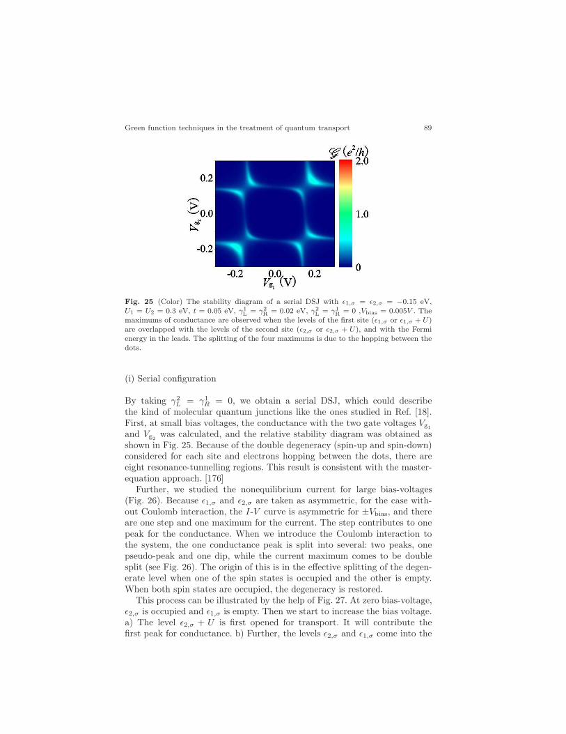
Green function techniques in the treatment of quantum transport 89
Fig. 25 (Color) The stability diagram of a serial DSJ with ǫ1,σ = ǫ2,σ = −0.15 eV,U1 = U2 = 0.3 eV, t = 0.05 eV, γ1
L = γ2R = 0.02 eV, γ2
L = γ1R = 0 ,Vbias = 0.005V . The
maximums of conductance are observed when the levels of the first site (ǫ1,σ or ǫ1,σ + U)are overlapped with the levels of the second site (ǫ2,σ or ǫ2,σ + U), and with the Fermienergy in the leads. The splitting of the four maximums is due to the hopping between thedots.
(i) Serial configuration
By taking γ2L = γ1
R = 0, we obtain a serial DSJ, which could describethe kind of molecular quantum junctions like the ones studied in Ref. [18].First, at small bias voltages, the conductance with the two gate voltages Vg1
and Vg2was calculated, and the relative stability diagram was obtained as
shown in Fig. 25. Because of the double degeneracy (spin-up and spin-down)considered for each site and electrons hopping between the dots, there areeight resonance-tunnelling regions. This result is consistent with the master-equation approach. [176]
Further, we studied the nonequilibrium current for large bias-voltages(Fig. 26). Because ǫ1,σ and ǫ2,σ are taken as asymmetric, for the case with-out Coulomb interaction, the I-V curve is asymmetric for ±Vbias, and thereare one step and one maximum for the current. The step contributes to onepeak for the conductance. When we introduce the Coulomb interaction tothe system, the one conductance peak is split into several: two peaks, onepseudo-peak and one dip, while the current maximum comes to be doublesplit (see Fig. 26). The origin of this is in the effective splitting of the degen-erate level when one of the spin states is occupied and the other is empty.When both spin states are occupied, the degeneracy is restored.
This process can be illustrated by the help of Fig. 27. At zero bias-voltage,ǫ2,σ is occupied and ǫ1,σ is empty. Then we start to increase the bias voltage.a) The level ǫ2,σ + U is first opened for transport. It will contribute thefirst peak for conductance. b) Further, the levels ǫ2,σ and ǫ1,σ come into the

90 D. A. Ryndyk, R. Gutierrez, B. Song, and G. Cuniberti
-2 0 20
5
10
-0.5
0.0
0.0 0.5 1.00.00
0.05J (
A)
Vbias (V)
G
(e2/h)
Fig. 26 (Color) Current and conductance vs. bias-voltage of a DSJ far from equilibriumwith parameters ǫ1,σ = 0.5 eV, ǫ2,σ = −0.5 eV, U1 = U2 = U = 0.2 eV, t = 0.07 eV,γ1L = γ2
R = 0.03 eV, Vg2= −Vg1
= Vbias/4 and VR = −VL = Vbias/2. The red curverepresents the current, while the blue the conductance. The inset is the blow-up for theconductance peak split. The dash and dot-dash curves are for current and conductancewith U = 0, respectively.
transport window between the left and the right Fermi levels, resulting inthe second peak. c) When the level ǫ1,σ + U comes into play, only a pseudo-peak appears. This is because there is only a little possibility for electronsto occupy the level ǫ1,σ under positive bias voltage. d) Levels ǫ2,σ + U andǫ1,σ meet, which results in electron resonant-tunnelling and leads to the firstmaximum of the current. Then a new level ǫ1,σ +U appears over the occupiedǫ1,σ due to the Coulomb interaction. e) The meeting of ǫ2,σ and ǫ1,σ results
Fig. 27 (Color) The processes involved in the transport characteristics in figure 26. ǫ1 ≡
ǫ1,σ , ǫ2 ≡ ǫ2,σ , The red line indicates electron resonant-tunnelling. a) The first conductancepeak. b) The second conductance peak. c) The pseudo-peak of conductance. d) The firstcurrent maximum, and the red line indicates resonant tunnelling of electrons. e) The secondcurrent maximum for electron resonant tunnelling. f) The dip of conductance.

Green function techniques in the treatment of quantum transport 91
in electron resonant tunnelling. It means that ǫ1,σ will be occupied, whichleads to the appearance of a new level ǫ1,σ +U . Then ǫ2,σ +U meets ǫ1,σ +Uand another resonant tunnelling channel is opened for electrons. The twochannels result in the second current maximum. f) finally, the level ǫ1,σ + Udisappears if the level ǫ1,σ is empty. This means that a dip appears in theconductance.
It should be noted that the characteristics of serial DSJ in Fig. 26 haveshowed some reasonable similarities to experiments of a single-moleculediode. [18]
(ii) Parallel configuration
If on the other hand, the two sites are symmetrically connected to the elec-trodes, possibly with a small inter-dot hopping, but with charging energiesU1 and U2 fixed to different scales for transport. The resulting stability dia-gram contains both interference effects for parallel pathways and an overlapof U1 and U2 stability diagrams, which we refer to a nesting characteristic.(see Fig. 28).
The physics of the weak lines in the figure can be understood by thehelp of charging effects. For simplicity, here we would ignore the site indexi. In the region of large positive gate voltage at zero bias voltage, ǫ↑ andǫ↓ are all empty, which means that the two levels are degenerate. Therefore
Fig. 28 (Color) Nested stability diagram of a parallel DSJ with parameters ǫ1,σ =−1.8 eV, ǫ2,σ = −0.3 eV, U1 = 3.6 eV, U2 = 0.6 eV t = 0.001 eV, γ1
L = γ1R = 0.04 eV,
γ2L = γ2
R = 0.05 eV, Vg2= Vg1
/2 = Vg/2 and VR = −VL = Vbias/2. See discussion in thetext.

92 D. A. Ryndyk, R. Gutierrez, B. Song, and G. Cuniberti
adding a bias voltage, first, there will be two channels (ǫ↑ and ǫ↓) openedfor current (thick lines). After then, one level ǫσ (spin-up or spin-down) isoccupied, while the other obtains a shift for Coulomb interaction: ǫσ → ǫσ+U .Therefore, when the bias voltage is further increased to make the Fermi-window boundary meeting level ǫσ + U , only one channel is opened for thecurrent, which results in the weak lines in Fig. 28, which is the characteristicof CB. The similar case appears in the region of large negative gate voltages.
Finally, we here introduced a powerful Ansatz for the lesser Green func-tion, which is consistent with both the Dyson-equation approach and theequation-of-motion approach. By using this Ansatz together with the stan-dard equation-of-motion technique for the retarded and advanced Green func-tions, we obtained the NEGF for both the single and the double site junctionsin the Coulomb blockade regime at finite voltages and calculated the trans-port observables. The method can be applied to describe self-consistentlytransport through single molecules with strong Coulomb interaction and ar-bitrary coupling to the leads.
To test our method, we here analyzed the CB stability diagrams for a SSJand a DSJ. Our results are all consistent with the results of experiments andthe master-equation approach. We showed, that the improved lesser Greenfunction gives better results for weak molecule-to-contact couplings, where acomparison with the master equation approach is possible.
For the serial configuration of a DSJ, such as a donor/acceptor rectifier,the I-V curves maintain a diode-like behavior, as it can be already inferredby coherent transport calculations. [265] Besides, we predict that as a resultof charging effects, one conductance peak will be split into three peaks andone dip, and one current maximum into two. For a DSJ parallel configuration,due to different charging energies on the two dot sites, the stability diagramsshow peculiar nesting characteristics.

Green function techniques in the treatment of quantum transport 93
4.2 Nonequilibrium vibrons
Though the electron-vibron model described in the Section II has a longhistory, the many questions it implies are not answered up to now. Whilethe isolated electron-vibron model can be solved exactly by the so-called po-laron or Lang-Firsov transformation [95, 96, 97], the coupling to the leadsproduces a true many-body problem. The inelastic resonant tunneling ofsingle electrons through the localized state coupled to phonons was first con-sidered in Refs. [98, 99, 100, 101]. There, the exact solution in the single-particle approximation was derived, ignoring completely the Fermi sea inthe leads. At strong electron-vibron couplings and weak couplings to theleads, satellites of the main resonant peak are formed in the spectral func-tion (Fig. 11). The number of the relevant side-bands is determined by thewell known Huang-Rhys factor [292] g = (λ/ω0)
2. The question which re-mains is whether these side-bands can be observed in the differential conduc-tance, when the coupling to all electrons in the leads should be taken intoaccount simultaneously. New theoretical treatments were presented recentlyin Refs. [134, 135, 136, 104, 138, 105, 106, 121, 120, 122, 117, 118, 126, 132,102, 103, 123, 288, 289, 107, 128, 129, 274, 127, 111, 140, 108, 109, 139, 290,84, 124, 275, 276, 164, 209, 125, 279, 278, 277, 133, 112].
In parallel, the theory of inelastic scanning tunneling spectroscopy wasdeveloped [161, 162, 113, 114, 115, 116, 163]. For a recent review of theelectron-vibron problem and its relation to charge transport at the molecularscale see Ref. [164]. Note the related problem of quantum shuttle [143, 145,149, 147].
Many interesting results by the investigation of quantum transport in thestrong electron-vibron coupling limit has been achieved with the help of themaster equation approach [104, 106, 107, 108, 109]. This method, however, isvalid only in the limit of very weak molecule-to-lead coupling and neglects allspectral effects, which are the most important at finite coupling to the leads.
4.2.1 Nonequilibrium Dyson-Keldysh method
(i) The model electron-vibron Hamiltonian
We use the minimal transport model described in the previous sections. Forconvenience, we present the Hamiltonian here once more. The full Hamilto-nian is the sum of the molecular Hamiltonian HM , the Hamiltonians of theleads HR(L), the tunneling Hamiltonian HT describing the molecule-to-lead
coupling, the vibron Hamiltonian HV including electron-vibron interactionand coupling of vibrations to the environment (describing dissipation of vi-brons)
H = HM + HV + HL + HR + HT . (405)

94 D. A. Ryndyk, R. Gutierrez, B. Song, and G. Cuniberti
A molecule is described by a set of localized states |α〉 with energies ǫαand inter-orbital overlap integrals tαβ by the following model Hamiltonian:
H(0)M =
∑
α
(ǫα + eϕα(t)) d†αdα +∑
α6=β
tαβd†αdβ . (406)
Vibrations and the electron-vibron coupling are described by the Hamil-tonian [121, 120, 122, 124] (h = 1)
HV =∑
q
ωqa†qaq +
∑
αβ
∑
q
λqαβ(aq + a†q)d
†αdβ . (407)
Here vibrations are considered as localized phonons and q is an index la-beling them, not the wave-vector. The first term describes free vibrons withthe energy ωq. The second term represents the electron-vibron interaction.We include both diagonal coupling, which describes a change of the electro-static energy with the distance between atoms, and the off-diagonal coupling,which describes the dependence of the matrix elements tαβ over the distancebetween atoms.
The Hamiltonians of the right (R) and left (L) leads read
Hi=L(R) =∑
kσ
(ǫikσ + eϕi)c†ikσcikσ , (408)
ϕi(t) are the electrical potentials of the leads. Finally, the tunneling Hamil-tonian
HT =∑
i=L,R
∑
kσ,α
(
Vikσ,αc†ikσdα + h.c.
)
(409)
describes the hopping between the leads and the molecule. A direct hoppingbetween two leads is neglected.
(ii) Keldysh-Dyson equations and self-energies
We use the nonequilibrium Green function (NGF) method, as introduced inSection III. The current in the left (i = L) or right (i = R) contact to themolecule is described by the expression
Ji=L,R =ie
h
∫
dǫ
2πTr
Γi(ǫ− eϕi)(
G<(ǫ) + f0i (ǫ− eϕi)
[
GR(ǫ) − GA(ǫ)])
,
(410)where f0
i (ǫ) is the equilibrium Fermi distribution function with chemical po-tential µi, and the level-width function is
Γi=L(R)(ǫ) = Γiαβ(ǫ) = 2π∑
kσ
Vikσ,βV∗ikσ,αδ(ǫ− ǫikσ).
Green function techniques in the treatment of quantum transport 95
The lesser (retarded, advanced) Green function matrix of a nonequilibrium
molecule G<(R,A) ≡ G<(R,A)αβ can be found from the Dyson-Keldysh equations
in the integral form
GR(ǫ) = GR0 (ǫ) + GR
0 (ǫ)ΣR(ǫ)GR(ǫ), (411)
G<(ǫ) = GR(ǫ)Σ<(ǫ)GA(ǫ), (412)
or from the corresponding equations in the differential form (see e.g. Refs. [123,124] and references therein).
HereΣR,< = Σ
R,<(T )L + Σ
R,<(T )R + ΣR,<(V ) (413)
is the total self-energy of the molecule composed of the tunneling (couplingto the left and right leads) self-energies
ΣR,<(T )j=L,R ≡ Σ
R,<(T )jαβ =
∑
kσ
V ∗jkσ,αGR,<jkσ Vjkσ,β
, (414)
and the vibronic self-energy ΣR,<(V ) ≡ ΣR,<(V )αβ .
For the retarded tunneling self-energy ΣR(T )i one obtains
ΣR(T )i (ǫ) = Λi(ǫ− eϕi) −
i
2Γi(ǫ− eϕi), (415)
where Λi is the real part of the self-energy, which usually can be included in
the single-particle Hamiltonian H(0)M , and Γi describes level broadening due
to coupling to the leads. For the corresponding lesser function one finds
Σ<(T )i (ǫ) = iΓi(ǫ− eϕi)f
0i (ǫ− eϕi). (416)
In the standard self-consistent Born approximation, using the Keldyshtechnique, one obtains for the vibronic self-energies [106, 121, 120, 122, 117,118, 164, 124]
ΣR(V )(ǫ) =i
2
∑
q
∫
dω
2π
(
MqGRǫ−ωMqDK
qω+
+MqGKǫ−ωMqDR
qω − 2DRqω=0M
qTr[
G<ω Mq
])
, (417)
Σ<(V )(ǫ) = i∑
q
∫
dω
2πMqG<
ǫ−ωMqD<qω , (418)
where GK = 2G<+GR−GA is the Keldysh Green function, and Mq ≡M qαβ .
If vibrons are noninteracting, in equilibrium, and non-dissipative, then thevibronic Green functions write:

96 D. A. Ryndyk, R. Gutierrez, B. Song, and G. Cuniberti
DR0 (q, ω) =
1
ω − ωq + i0+− 1
ω + ωq + i0+, (419)
D<0 (q, ω) = − 2πi
[
(f0B(ωq) + 1)δ(ω + ωq) + f0
B(ωq)δ(ω − ωq)]
, (420)
where the equilibrium Bose distribution function is
f0B(ω) =
1
exp (ω/T )− 1. (421)
In the Migdal model the retarded vibron function is calculated from theDyson-Keldysh equation
DR(q, ω) =2ωq
ω2 − ω2q − 2ωqΠR(q, ω)
, (422)
where Π(q, ω) is the polarization operator (boson self-energy). The equationfor the lesser function (quantum kinetic equation in the integral form) is
(ΠRqω −ΠA
qω)D<qω − (DR
qω −DAqω)Π<
qω = 0, (423)
this equation in the stationary case considered here is algebraic in the fre-quency domain.
The polarization operator is the sum of two parts, environmental and
electronic: ΠR,<qω = Π
R,<(env)qω +Π
R,<(el)qω .
The environmental equilibrium part of the polarization operator can beapproximated by the simple expressions
ΠR(env)(q, ω) = − i
2γqsign(ω), (424)
Π<(env)(q, ω) = −iγqf0B(ω)sign(ω), (425)
where γg is the vibronic dissipation rate, and f0B(ω) is the equilibrium Bose-
Einstein distribution function.The electronic contribution to the polarization operator within the SCBA
is
ΠR(el)(q, ω) = −i∫
dǫ
2πTr(
MqG<ǫ MqGA
ǫ−ω + MqGRǫ MqG<
ǫ−ω
)
, (426)
Π<(el)(q, ω) = −i∫
dǫ
2πTr(
MqG<ǫ MqG>
ǫ−ω
)
. (427)
We obtained the full set of equations, which can be used for numericalcalculations.

Green function techniques in the treatment of quantum transport 97
4.2.2 Single-level model: spectroscopy of vibrons
The isolated single-level electron-vibron model is described by the Hamilto-nian
HM+V = (ǫ0 + eϕ0)d†d+ ω0a
†a+ λ(
a† + a)
d†d, (428)
where the first and the second terms describe the free electron state and thefree vibron, and the third term is electron-vibron minimal coupling interac-tion.
The electrical potential of the molecule ϕ0 plays an important role intransport at finite voltages. It describes the shift of the molecular level bythe bias voltage, which is divided between the left lead (tip), the right lead(substrate), and the molecule as ϕ0 = ϕR + η(ϕL − ϕR) [293]. We assumethe simplest linear dependence of the molecular potential (η = const), butits nonlinear dependence [294] can be easily included in our model.
Here we assume, that the vibrons are in equilibrium and are not excitedby the current, so that the self-consistent Born approximation is a goodstarting point. The vibron Green function are assumed to be equilibriumwith the broadening defined by the external thermal bath, see for detailsRefs. [120, 117, 118, 164, 124].
For the single-level model all equations are significantly simplified. Com-bining JL and JR the expression for the current can be written for energyindependent ΓL(R) (wide-band limit) as
J =e
h
ΓLΓR
ΓR + ΓL
∫
dǫA(ǫ)[
f0(ǫ− eϕL) − f0(ǫ− eϕR)]
. (429)
It looks as simple as the Landauer-Buttiker formula, but it is not trivial,because the spectral density A(ǫ) = −2ImGR(ǫ) now depends on the distri-
0 2 4 6 8 10ε
A(ε
)
0 2 4 6 8ε
Fig. 29 (Color online) Spectral function at different electron-vibron couplings: λ/ω0 = 0.4
(black), λ/ω0 = 1.2 (blue, dashed), and λ/ω0 = 2 (red); at ǫ0/ω0 = 5, ΓL/ω0 = ΓR/ω0 =0.1. In the insert the spectral function at λ/ω0 = 1.2 is shown at finite voltage, when thelevel is partially filled. Energies are in units of hω0.

98 D. A. Ryndyk, R. Gutierrez, B. Song, and G. Cuniberti
Fig. 30 Differential conductance of a symmetric junction (η = 0.5, ΓR = ΓL) at differentmolecule-to-lead coupling, from ΓL/ω0 = 0.1 (lower curve) to ΓL/ω0 = 10 (upper curve),λ/ω0 = 1, ǫ0/ω0 = 2. Voltage is in the units of hω0/e.
bution function of the electrons in the fluctuating molecule and hence theapplied voltage, ϕL = −ϕR = V/2 [123]. Indeed, GR(ǫ) can be found from(201)
GR(ǫ) =1
ǫ− ǫ0 −ΣR(V )(ǫ) + i(ΓL + ΓR)/2, (430)
where ΣR(V )(ǫ) is a functional of the electron distribution function insidea molecule. Actually, the lesser function G<(ǫ) is used in the quantum ki-netic formalism as a distribution function. In the single-level case the usualdistribution function can be introduced through the relation
G<(ǫ) = iA(ǫ)f(ǫ). (431)
Note the essential difference between symmetric (ΓL = ΓR) and asymmet-ric junctions. It is clear from the noninteracting solution of the transportproblem. Neglecting for a moment the vibron self-energies, we obtain thenoninteracting distribution function
f(ǫ) =ΓLf
0L(ǫ− eϕL) + ΓRf
0R(ǫ− eϕR)
ΓL + ΓR. (432)
For strongly asymmetric junctions (e.g. ΓL ≪ ΓR) the distribution functionremains close to the equilibrium function in the right lead f0
R(ǫ− eϕR), thusessentially simplifying the solution. While for symmetric junctions the dis-tribution function has the double-step form and is very different from theequilibrium one.
A typical example of the spectral function at zero voltage is shown inFig. 29. At finite voltage it should be calculated self-consistently. In the insert

Green function techniques in the treatment of quantum transport 99
Fig. 31 Differential conductance of an asymmetric junction (η = 0, ΓR = 20ΓL) atdifferent molecule-to-lead coupling, from ΓR/ω0 = 0.2 (lower curve) to ΓR/ω0 = 4 (uppercurve), λ/ω0 = 2, ǫ0/ω0 = 5. The voltage is in the units of hω0/e
the spectral function of the symmetric junction at finite voltage is shown, itis changed essentially because the distribution function is changed.
Let us discuss a general picture of the vibronic transport in symmetricand asymmetric single-molecule junctions, provided in experiments with themolecular bridges and STM-to-molecule junctions, respectively. The differen-tial conductance, calculated at different molecule-to-lead coupling, is shownin Fig. 30 (symmetric) and Fig. 31 (asymmetric). At weak coupling, the vi-bronic side-band peaks are observed, reproducing the corresponding peaks inthe spectral function. At strong couplings the broadening of the electronicstate hides the side-bands, and new features become visible. In the symmet-ric junction, a suppression of the conductance at V ≃ ±hω0 takes place asa result of inelastic scattering of the coherently transformed from the leftlead to the right lead electrons. In the asymmetric junction (Fig. 31), theusual IETS increasing of the conductance is observed at a negative voltageV ≃ −hω0, this feature is weak and can be observed only in the incoherenttail of the resonant conductance. We conclude, that the vibronic contribu-tion to the conductance can be distinguished clearly in both coherent andtunneling limits.
Now let us discuss the particular situation of STS experiments [32, 33, 35,36]. Here we concentrate mainly on the dependence on the tip-to-molecule dis-tance [33]. When the tip (left lead in our notations) is far from the molecule,the junction is strongly asymmetric: ΓL ≪ ΓR and η → 0, and the con-ductance is similar to that shown in Fig. 31. When the tip is close to themolecule, the junction is approximately symmetric: ΓL ≈ ΓR and η ≈ 0.5,and the conductance curve is of the type shown in Fig. 30. We calculated thetransformation of the conductance from the asymmetric to symmetric case(Fig. 32). It is one new feature appeared in asymmetric case due to the factthat we started from a finite parameter η = 0.2 (in the Fig. 31 η = 0), namely

100 D. A. Ryndyk, R. Gutierrez, B. Song, and G. Cuniberti
Fig. 32 (Color) Differential conductance at different molecule-to-STM coupling (see thetext), from asymmetric junction with ΓL/ω0 = 0.025, ΓR/ω0 = 0.5 and η = 0.2 (lowercurve, blue thick line) to symmetric junction with ΓL/ω0 = ΓR/ω0 = 0.5 and η = 0.5(upper curve, red thick line), λ/ω0 = 1, ǫ0/ω0 = 2. Voltage is in the units of hω0/e
a single peak at negative voltages, which is shifted to smaller voltage in thesymmetric junction. The form and behavior of this peak is in agreement withexperimental results [33].
In conclusion, at weak molecule-to-lead (tip, substrate) coupling the usualvibronic side-band peaks in the differential conductance are observed; atstronger coupling to the leads (broadening) these peaks are transformed intostep-like features. A vibronic-induced decreasing of the conductance withvoltage is observed in high-conductance junctions. The usual IETS feature(increasing of the conductance) can be observed only in the case of low off-resonant conductance. By changing independently the bias voltage and thetip position, it is possible to determine the energy of molecular orbitals andthe spectrum of molecular vibrations. In the multi-level systems with strongelectron-electron interaction further effects, such as Coulomb blockade andKondo effect, could dominate over the physics which we address here; theseeffects have to be included in a subsequent step.
4.2.3 Multi-level model: nonequilibrium vibrons
Basically there are two main nonequilibrium effects: the electronic spectrummodification and excitation of vibrons (quantum vibrations). In the weakelectron-vibron coupling case the spectrum modification is usually small(which is dependent, however, on the vibron dissipation rate, temperature,etc.) and the main possible nonequilibrium effect is the excitation of vibronsat finite voltages. We have developed an analytical theory for this case [124].This theory is based on the self-consistent Born approximation (SCBA),
Green function techniques in the treatment of quantum transport 101
which allows to take easily into account and calculate nonequilibrium dis-tribution functions of electrons and vibrons.
If the mechanical degrees of freedom are coupled strongly to the envi-ronment (dissipative vibron), then the dissipation of molecular vibrations isdetermined by the environment. However, if the coupling of vibrations to theleads is weak, we should consider the case when the vibrations are excited bythe current flowing through a molecule, and the dissipation of vibrations isalso determined essentially by the coupling to the electrons. Here , we showthat the effects of vibron emission and vibronic instability are importantespecially in the case of electron-vibron resonance.
We simplify the equations and obtain some analytical results in the vi-bronic quasiparticle approximation, which assumes weak electron-vibron cou-pling limit and weak external dissipation of vibrons:
γ∗q = γq − 2ImΠR(ωq) ≪ ωq. (433)
So that the spectral function of vibrons can be approximated by the Dirac δ,and the lesser function reads
D<(q, ω) = −2πi [(Nq + 1)δ(ω + ωq) +Nqδ(ω − ωq)] , (434)
where Nq is (nonequilibrium) number of vibrations in the q-th mode. So,in this approximation the spectrum modification of vibrons is not takeninto account, but the possible excitation of vibrations is described by thenonequilibrium Nq. The dissipation of vibrons is neglected in the spectralfunction, but is taken into account later in the kinetic equation for Nq.A similar approach to the single-level problem was considered recently in[113, 114, 115, 116, 106, 117, 118]. The more general case with broadenedequilibrium vibron spectral function seems to be not very interesting, be-cause in this case vibrons are not excited. Nevertheless, in the numericalcalculation it can be easy taken into consideration.
From the general quantum kinetic equation for vibrons, we obtain in thislimit
Nq =γqN
0q − ImΠ<(ωq)
γq − 2ImΠR(ωq). (435)
This expression describes the number of vibrons Nq in a nonequilibriumstate, N0
q = f0B(ωq) is the equilibrium number of vibrons. In the linear ap-
proximation the polarization operator is independent ofNq and −2ImΠR(ωq)describes additional dissipation. Note that in equilibrium Nq ≡ N0
q because
ImΠ<(ωq) = 2ImΠR(ωq)f0B(ωq). See also detailed discussion of vibron emis-
sion and absorption rates in Refs. [113, 114, 115, 116].For weak electron-vibron coupling the number of vibrons is close to equilib-
rium and is changed because of vibron emission by nonequilibrium electrons,Nq is roughly proportional to the number of such electrons, and the distri-bution function of nonequilibrium electrons is not change essentially by the

102 D. A. Ryndyk, R. Gutierrez, B. Song, and G. Cuniberti
interaction with vibrons (perturbation theory can be used). The situationchanges, however, if nonequilibrium dissipation −2ImΠR(ωq) is negative. Inthis case the number of vibrons can be essentially larger than in the equi-librium case (vibronic instability), and the change of electron distributionfunction should be taken into account self-consistently.
In the stationary state the nonlinear dissipation rate
γ∗q = γq − 2ImΠR(ωq) (436)
is positive, but the nonequilibrium contribution to dissipation −2ImΠR(ωq)remains negative.
Additionally to the vibronic quasiparticle approximation, the electronicquasiparticle approximation can be used when the coupling to the leads isweak. In this case the lesser function can be parameterized through the num-ber of electrons Fη in the eigenstates of the noninteracting molecular Hamil-
tonian H(0)M
G<αβ = i
∑
γη
AαγSγηFηS−1ηβ , (437)
we introduce the unitary matrix S, which transfer the Hamiltonian H ≡H
(0)Mαβ into the diagonal form H = S−1HS, so that the spectral function of
this diagonal Hamiltonian is
Aδη(ǫ) = 2πδ(ǫ− ǫδ)δδη, (438)
where ǫδ are the eigenenergies.
-5 0 5Voltage
Curr
ent (a
rb.u
nits
)
0.00
0.02
0.04
0.06
NV
Fig. 33 (Color) Vibronic emission in the symmetric multilevel model: voltage-currentcurve, differential conductance, and the number of excited vibrons in the off-resonant(triangles) and resonant (crosses) cases (details see in the text).

Green function techniques in the treatment of quantum transport 103
Note that in the calculation of the self-energies and polarization operatorswe can not use δ-approximation for the spectral function (this is too roughand results in the absence of interaction out of the exact electron-vibronresonance). So that in the calculation we use actually (437) with broad-ened equilibrium spectral function. This approximation can be systematicallyimproved by including nonequilibrium corrections to the spectral function,which are important near the resonance. It is important to comment thatfor stronger electron-vibron coupling vibronic side-bands are observed in thespectral function and voltage-current curves at energies ǫδ ± nωq, we do notconsider these effects in the rest of our paper and concentrate on resonanceeffects.
After correspondingly calculations we obtain finally
Nq =γqN
0q −∑ηδ κηδ(ωq)Fη(Fδ − 1)
γq −∑
ηδ κηδ(ωq)(Fη − Fδ), (439)
where coefficients κηδ are determined by the spectral function and electron-vibron coupling in the diagonal representation
κηδ(ωq) =
∫
dǫ
2πM q
ηδAδδ(ǫ− ωq)MqδηAηη(ǫ), (440)
Fη =ΓLηηf
0Lη+ΓRηηf
0Rη+
∑
qη
[
ζ−qηδ FδNq+ζ+q
ηδ Fδ(1+Nq)]
ΓLηη+ΓRηη+∑
qη
[
ζ−qηδ (1−Fδ+Nq)+ζ
+qηδ (Fδ +Nq)
] , (441)
ζ±qηδ = M q
ηδAδδ(ǫη ± ωq)Mqδη, (442)
here Γiηη and f0iη are the level width matrix in the diagonal representation
and Fermi function at energy ǫη − eϕi.These kinetic equations are similar to the usual golden rule equations, but
are more general.Now let us consider several examples of vibron emission and vibronic in-
stability.First we consider the most simple case, when the instability is not possible
and only vibron emission takes place. This corresponds to a negative imagi-nary part of the electronic polarization operator: ImΠR)(ωq) < 0. From theEq. (440) one can see that for any two levels with the energies ǫη > ǫδ the
coefficient κηδ is larger than κδη, because the spectral function Aδδ(ǫ) hasa maximum at ǫ = ǫδ. The contribution of κηδ(ωq)(Fη − Fδ) is negative ifFη < Fδ. This takes place in equilibrium, and in nonequilibrium for trans-port through symmetric molecules, when higher energy levels are populatedafter lower levels. The example of such a system is shown in Fig. 33. Herewe consider a simple three-level system (ǫ1 = 1, ǫ2 = 2, ǫ3 = 3) coupledsymmetrically to the leads (ΓLη = ΓRη = 0.01). The current-voltage curveis the same with and without vibrations in the case of symmetrical coupling

104 D. A. Ryndyk, R. Gutierrez, B. Song, and G. Cuniberti
-5 0 5Voltage
Curr
en
t (a
rb. u
nits
)
0.0
0.2
0.4
0.6
NV
Fig. 34 (Color) Vibronic instability in an asymmetric multilevel model: voltage-currentcurve, differential conductance, and the number of excited vibrons (crosses). Dashed lineshow the voltage-current curve without vibrons (details see in the text).
-2 -1 0 1 2Voltage
Curr
ent (a
rb.u
nits
)
0.0
0.1
0.2
0.3
NV
Fig. 35 (Color) Floating level resonance: voltage-current curve and the number of excitedvibrons (crosses). Dashed line show the voltage-current curve without vibrons (details seein the text).
to the leads and in the weak electron-vibron coupling limit (if we neglectchange of the spectral function). The figure shows how vibrons are excited,the number of vibrons NV in the mode with frequency ω0 is presented in twocases. In the off-resonant case (green triangles) NV is very small comparingwith the resonant case (ω0 = ǫ2− ǫ1, red crosses, the vertical scale is changedfor the off-resonant points). In fact, if the number of vibrons is very large, thespectral function and voltage-current curve are changed. We shall considerthis in a separate publication.
Now let us consider the situation when the imaginary part of the electronicpolarization operator can be positive: ImΠR(ωq) > 0. Above we considered

Green function techniques in the treatment of quantum transport 105
the normal case when the population of higher energy levels is smaller thanlower levels. The opposite case F2 > F1 is known as inversion in laser physics.Such a state is unstable if the total dissipation γ∗q (436) is negative, which ispossible only in the nonstationary case. As a result of the instability, a largenumber of vibrons is excited, and in the stationary state γ∗q is positive. Thiseffect can be observed for transport through asymmetric molecules, whenhigher energy levels are populated before lower levels. The example of a suchsystem is shown in Fig. 34. It is the same three-level system as before, butthe first and second levels are coupled not symmetrically to the leads (ΓL1 =0.001, ΓR1 = 0.1, ΓL2 = 0.1, ΓR2 = 0.001). The vibron couple resonantlythese levels (ωq = ǫ2 − ǫ1). The result is qualitatively different from thesymmetrical case. The voltage-current curve is now asymmetric, a large stepcorresponds to the resonant level with inverted population.
Note the importance of the off-diagonal electron-vibron coupling for theresonant effects. If the matrix M in the eigen-state representation is diagonal,there is no resonant coupling between different electronic states.
Finally, let us consider the important case, when initially symmetricmolecule becomes asymmetric when the external voltage is applied. The rea-son for such asymmetry is simply that in the external electric field left andright atoms feel different electrical potentials and the position of the levels
ǫα = ǫ(0)α + eϕα is changed (float) with the external voltage. The example of
a such system is shown in Fig. 35. Here we consider a two-level system, onelevel is coupled electrostatically to the left lead ǫ1 ∝ ϕL, the other level to theright lead ǫ2 ∝ ϕR, the tunneling coupling to the leads also is not symmetri-cal (ΓL1 = 0.1, ΓR1 = 0.001, ΓL2 = 0.001, ΓR2 = 0.1). The frequency of thevibration, coupling these two states, is ω0 = 1. When we sweep the voltage,a peak in the voltage-current curve is observed when the energy differenceǫ1 − ǫ2 ∝ eV is going through the resonance ǫ1 − ǫ2 ≈ ω0.
106 D. A. Ryndyk, R. Gutierrez, B. Song, and G. Cuniberti
4.3 Coupling to a vibrational contiuum: dissipation
and renormalization
4.3.1 The model Hamiltonian
In the previous section we have dealt with a simple, but nevertheless phys-ically rich, model describing the interaction of an electronic level with somespecific vibrational mode confined to the quantum dot. We have seen howto apply in this case the Keldysh non-equilibrium techniques described inSection III within the self-consistent Born and Migdal approximations. Thelatter are however appropriate for the weak coupling limit to the vibrationaldegrees of freedom. In the opposite case of strong coupling, different tech-niques must be applied. For equilibrium problems, unitary transformationscombined with variational approaches can be used, in non-equilibrium onlyrecently some attempts were made to deal with the problem. [139]
In this section we will consider the case of a multi-level electronic systemin interaction with a bosonic bath [288, 289]. We will use unitary transforma-tion techniques to deal with the problem, but will only focus on the low-biastransport, so that strong non-equilibrium effects can be disregarded. Our in-terest is to explore how the qualitative low-energy properties of the electronicsystem are modified by the interaction with the bosonic bath. We will see thatthe existence of a continuum of vibrational excitations (up to some cut-off fre-quency) dramatically changes the analytic properties of the electronic Greenfunction and may lead in some limiting cases to a qualitative modificationof the low-energy electronic spectrum. As a result, the I-V characteristics atlow bias may display “metallic” behavior (finite current) even if the isolatedelectronic system does exhibit a band gap. The model to be discussed belowhas been motivated by the very exciting electrical transport measurementson short poly(dG)-poly(dC) DNA molecular wires carried out at the groupof N. Tao some time ago [60]. Peculiar in these experiments was the largemeasured currents -up to 150 nA at 0.8 V- at low voltages, which stood instrong contrast to the usually accepted view that DNA should behave as aninsulator at low applied bias. Further, a power-law length scaling of the linearconductance with increasing wire length was demonstrated, indicating thatlong-range charge transport was possible. Since the experiments were carriedout in an aqueous solution, the possibility of a solvent-induced modificationof the low-energy transport properties of the wire lied at hand, althoughadditional factors like internal vibrations could also play a role.
The proposed model is based on an earlier work [286] and assumes, withina minimal tight-binding picture, that the DNA electronic states can be quali-tatively classified into extended (conducting) and localized (non-conducting)states. The former may correspond e.g. to the π-orbital stack of the basepairs, the latter to energetically deeper lying (w.r.t. the frontier orbitals)base-pair states or sugar-phosphate backbone states. A further assumption is

Green function techniques in the treatment of quantum transport 107
t
c c c1 2 3 Nc
1 2 3 N
t
. . . . . .
. . . . . .||
| |
b b b bL R
phonon bath
Fig. 36 (Color) Schematic drawing of a DNA molecular wire in contact with a dissipativeenvironment. The central chain (extended states) with N sites is connected to semiinfinite
left (L) and right (R) electronic reservoirs. The bath only interacts with the side chainsites (c), which we call for simplicity backbone sites, but which collectively stay for non-conducting, localized electronic states. The Hamiltonian associated with this model is givenby Eqs. (443), (444), and (445) in the main text.
that any modification of the conducting states through the environment onlytakes place through a coupling to the non-conducting set. The tight-bindingelectronic Hamiltonian for N sites can then be written as (see also Fig. 36):
Hel = ǫb∑
j
b†jbj − t||∑
j
[
b†jbj+1 + H.c.]
+ ǫ∑
j
c†jcj
− t⊥∑
j
[
b†jcj + H.c.]
= HC + Hb + HC-b. (443)
Hereby HC and Hb are the Hamiltonians of the extended and localizedstates (called in what follows “backbone” states for simplicity), respectively,and HC-b is the coupling between them. t|| and t⊥ are hopping integralsalong the central chain (extended states) and between the localized statesand the central chain, respectively. If not stated otherwise, the on-site ener-gies will be later set equal to zero to simplify the calculations. Notice thatthis model displays a gap in the electronic spectrum roughly proportional tothe transversal coupling t⊥. This can be easely seen by looking at the limitN → ∞ which leads to a periodic system. In this case, the Hamiltonian canbe analytically diagonalized and two energy dispersion curves are obtained,
which are given by E±(k) = t|| cos(k) ±√
t2⊥ + t2|| cos2(k). The direct gap
between the two bands is simply δ = 2√
t2⊥ + t2||. Since this model further
shows electron-hole symmetry, two electronic manifolds (bands in the limitof N → ∞) containing N states each, are symmetrically situated around theFermi level, which is taken as the zero of energy.
The gap is obviously temperature independent and furthermore it is ex-pected that transport at energies E < δ will be strongly suppressed due to

108 D. A. Ryndyk, R. Gutierrez, B. Song, and G. Cuniberti
the absence of electronic states to suport charge propagation. As a result,the linear conductance should display a strong exponential dependence as afunction of the chain length N . In view of this behavior, an immediate issuethat arises is how stable this electronic structure, i.e. two electronic manifoldsseparated by a gap, is against the coupling to an environment. This is an issuewhich reaches farther than the problem of charge transport in DNA wires,since it addresses the interaction of an open quantum mechanical system witha countable number of electronic energy levels to a continuum of states (“uni-verse”). A generic example of such a situation is the measurement process inquantum mechanics. It is well-known that the interaction with complex envi-ronments is a source of dissipation and decoherence in quantum mechanicalsystems. [71] Concerning more specifically the case of DNA (and proteins),there is broad experimental evidence that the molecule dynamics follows thesolvent dynamics over a broad temperature range. Especially, conformationalchanges, low-energy vibrational excitations and the corresponding tempera-ture dependences turn out to be very sensitive to the solvents dynamics. [295]We will thus consider the vibrational degrees of freedom of counterions andhydration shells of the solvent as a dynamical bath able to break the elec-tronic phase coherence and additionally to act as a dissipative environment.We do not consider specific features of the environment but represent it in ageneric way by a bosonic bath of M harmonic oscillators. Then, the previousHamiltonian can be extended to:
HW = Hel +∑
α
ΩαB†αBα +
∑
α,j
λαc†jcj(Bα +B†α) = Hel +HB +Hc-B, (444)
where HB and Hc-B are the phonon bath Hamiltonian and the (localized)state-bath interaction, respectively. Bα is a bath phonon operator and λα
denotes the electron-phonon coupling. Note that we assume a local couplingof the bath modes to the electronic density at the side chain. Later on, thethermodynamic limit (M → ∞) in the bath degrees of freedom will be carriedout and the corresponding bath spectral density introduced, so that at thisstage we do not need to further specify the set of bath frequencies Ωα andcoupling constants λα. Obviously, the bath can be assumed to be in thermalequilibrium and be described by a canonical partition function.
To complete the formulation of the model, we have to include the inter-action of the system with electronic reservoirs in order to describe chargetransport along the same lines as before. We assume, as usual, a tunnel-typeHamiltonian with the form:
H = HW +∑
k∈L,R,σ
ǫkσd†kσdkσ +
∑
k∈L,σ
(Vk,1 d†kσ b1 + H.c.)
+∑
k∈R,σ
(Vk,N d†kσ bN + H.c.) = HW + HL/R + HL-C + HR-C. (445)

Green function techniques in the treatment of quantum transport 109
The Hamiltonian of Eq. (445) is the starting point of our investigation.For a weak charge-bath coupling, a perturbative approach similar to thesecond order Born approximation, as described in the previous section can beapplied. We expect, however, qualitative new effects rather in the oppositelimit of strong coupling to the bath. To deal with this problem, a unitarytransformation, the Lang-Firsov (LF) transformation, can be performed onthe Hamiltonian of Eq. (445), which allows to eliminate the linear charge-vibron interaction Hc-B. In the limiting case of an isolated system with asingle electron (or hole) this transformation becomes exact and allows for afull decoupling of electronic and vibronic propagators, see e.g. Ref. [97]. Inthe present case, this transformation is not exact and further approximationshave to be introduced in order to make the problem tractable.
The generator of the LF transformation is given by
S =∑
α,j
(λα/Ωα)c†jcj(Bα −B†α)
and S† = −S. In the transformed Hamiltonian H = e SHe−S the linearcoupling to the bath is eliminated. One should notice that in H only the“backbone” part of the Hamiltonian is modified since the conducting stateoperators bℓ as well as the lead operators dkσ are invariant with respect tothe above transformation. The new Hamiltonian reads:
H = HC + HL/R + HB + HL/R-C + (ǫ−∆)∑
j
c†jcj − t⊥∑
j
[
b†jcjX + H.c.]
,
X = exp
[
∑
α
λα
Ωα(Bα −B†α)
]
, ∆ =∑
α
λ2α
Ωα. (446)
As a result of the LF we get a shift of the onsite energies (polaron shiftor reorganization energy in electron transfer theory) and a renormalizationof both the tunneling and of the transversal coupling Hamiltonian via thebosonic operators X . There is also an additional electron-electron interactionterm which we will not be concerned with in the remaining of this section andis thus omitted. Since we are mainly interested in qualitative statements, wewill assume the wide-band approximation in the coupling to the electrodeswhich is equivalent to substituting the electrode self-energies by a purelyimaginary constant, i.e. ΣL,R ≈ −iΓL,R. We are thus not interested in specificfeatures of the electrode electronic structure.
To further proceed, let us now introduce two kinds of retarded thermalGreen functions related to the central chain Gjℓ(t) and to the “backbones”Pjℓ(t), respectively (taking h = 1):

110 D. A. Ryndyk, R. Gutierrez, B. Song, and G. Cuniberti
Gjℓ(t, t′) = −iΘ(t− t′)
⟨
[
bj(t), b†ℓ(t′)]
+
⟩
, (447)
Pjℓ(t, t′) = −iΘ(t− t′)
⟨
[
cj(t)X (t), c†ℓ(t′)X †(t′)
]
+
⟩
,
where Θ is the Heaviside function. Notice that the P -Green function doe nothave a pure electronic character but also contains the bath operators X . Fora full out-of-equilibrium calculation, the full Keldysh formalism includinglesser- and greater-GF would also be needed. However, as we will brieflyshow below, the final expression for the electrical current at low appliedvoltages and for small transversal coupling t⊥ will only include the retardedpropagators.
We now use the equation of motion technique (EOM) to obtain an expres-sion for the GF Gjℓ(t). We first remark that in the time domain two EOMcan be written, depending on which time argument in the double-time GFthe time derivative will act. One thus obtains in general:
i ∂tG(t, t′) =⟨
[
b(t), b†(t′)]
+
⟩
δ(t− t′) + (([b(t), H ] |b†(t′))).
G(t, t′)[−i ∂t′ ] =⟨
[
b(t), b†(t′)]
+
⟩
δ(t− t′) − ((b(t)|[
b†(t′), H]
)).
The EOM for the GF Gjℓ(t) reads then in the energy space:
∑
n
[
G−10 (E)
]
ℓnGnj(E) = δℓj − t⊥((cℓX|b†j)) (448)
[
G−10 (E)
]
ℓn= (E − ǫb)δnℓ + t||(δn,ℓ+1 + δn,ℓ−1) −ΣLδℓ1δn1 −ΣRδℓNδnN
ΣL(R) =∑
k∈L(R)
|Vk,1(N)|2E − ǫk + i 0+
≈ −iΓL,R
In the next step, EOM for the “right” time argument t′ of the GFZXℓj (t, t
′)((cℓ(t)X (t)|b†j(t′))) can be written. This leads to:
∑
m
ZXℓm(E)[
G−10 (E)
]
mj= −t⊥((cℓX|c†jX †)) = −t⊥Pℓj(E) (449)
Inserting Eq. (449) into Eq. (448) we arrive at the matrix equation:
G(E) = G0(E) + G0(E)ΣB(E)G0(E),
which can be transformed into a Dyson-like equation when introducing theirreducible part ΣB(E) = Σirr
B (E) + ΣirrB (E)G0(E)Σirr
B (E) + . . . :
G(E) = G0(E) + G0(E)ΣirrB (E)G(E), (450)

Green function techniques in the treatment of quantum transport 111
or equivalently:
G−1(E) = G−10 (E) − t2⊥P(E) (451)
G−10 (E) = E1−HC −ΣL(E) −ΣR(E).
ΣirrB (E) = t2⊥P(E) is the crucial contribution to the GF since it contains
the influence of the bosonic bath. Note that ΣirrB (E) includes the transversal
hopping t⊥ to all orders, the leading one being t2⊥.In the next step, an expression for the electrical current flowing through
the system must be derived. Using the results of Sec. 2, we can directly writethe following expression:
I =2e
h
∫
dE Tr(fL(E) − fR(E)) t(E)
+ t2⊥2e
h
∫
dE
Tr[Σ>L P< − Σ<
L P>] − (L↔ R)
. (452)
The first summand has the same form as Landauer’s expression for the cur-rent with an effective transmission function t(E) = Tr[G†ΓRGΓR]. However,the reader should keep in mind that the GFs appearing in this expression docontain the full dressing by the bosonic bath and hence, t(E) does not de-scribe elastic transport. The remaining terms contain explicitly contributionsfrom the bath. It can be shown after some transformations that the leadingterm is proportional to (t2⊥)2 so that within a perturbative approach in t⊥and at low bias it can be approximately neglected. We therefore remian withthe exression I = 2e
h
∫
dE Tr(fL(E) − fR(E)) t(E) to obtain the current.To remain consistent with this approximation, the bath selfenergy should
also be treated to order t2⊥, more explicitly:
Pℓj(t, t′) = ((cℓ(t)X (t)|c†j(t′)X †(t′)))
≈ −i θ(t− t′)⟨
cℓ(t)c†j(t′)⟩
⟨
X (t)X †(t′)⟩
+⟨
c†j(t′)cℓ(t)
⟩
⟨
X †(t′)X (t)⟩
≈ −i δℓjθ(t− t′)⟨
cj(t)c†j(t′)⟩
⟨
X (t)X †(t′)⟩
+⟨
c†j(t′)cj(t)
⟩
⟨
X †(t′)X (t)⟩
= −i δℓjθ(t− t′)e−i (ǫ−∆) t
(1 − fc)e−Φ(t) + fce
−Φ(−t)
. (453)
In the previous expression we have replaced the full averages of the “back-bone” operators by their zero order values (free propagators). e−Φ(t) =⟨
X (t)X †(0)⟩
Bis a dynamical bath correlation function to be specified later
on. The average 〈·〉B is performed over the bath degrees of freedom. fc is theFermi function at the backbone sites. In what follows we consider the case ofempty sites by setting fc = 0. The Fourier transform Pℓj(E) reads then:

112 D. A. Ryndyk, R. Gutierrez, B. Song, and G. Cuniberti
Pℓj(E) = −i δℓj
∫ ∞
0
dt e i (E+i 0+)t e−i (ǫ−∆) t[
(1 − fc)e−Φ(t) + fce
−Φ(−t)]
(454)In order to get closed expressions for the bath thermal averages it is ap-
propriate to introduce a bath spectral density [71] defined by :
J(ω) =∑
α
λ2αδ(ω −Ωα) = J0(
ω
ωc)se−ω/ωcΘ(ω), (455)
where ωc is a cut-off frequency related to the bath memory time τc ∼ ω−1c .
It is easy to show that the limit ωc → ∞ corresponds to a Markovian bath,i.e. J(t) ∼ J0δ(t). Using this Ansatz, Φ(t) can be written as:
Φ(t) =
∫ ∞
0
dωJ(ω)
ω2
[
1 − e−i ωt + 21 − cosωt
e βω − 1
]
. (456)
Although the integral can be performed analytically [71], we consider Φ(t) insome limiting cases where it is easier to work directly with Eq. (456).
4.3.2 Limiting cases
We use now the results of the foregoing section to discuss the electronictransport properties of our model in some limiting cases for which analyticexpressions can be derived. We will discuss the mean-field approximationand the weak-coupling regime in the electron-bath interaction as well as toelaborate on the strong-coupling limit. Farther, the cases of ohmic (s = 1)and superohmic (s = 3) spectral densities are treated.
(i) Mean-field approximation
The mean-field approximation is the simplest one and neglects bath fluc-tuations contained in P (E). The MFA can be introduced by writing thephonon operator X as 〈X 〉B + δX in HC-c in Eq. (446), i.e. HMF
C-b =
−t⊥∑
j
[
b†jcj 〈X 〉B + H.c.]
+ O(δX ). As a result a real, static and tempera-
ture dependent term in Eq. (451) is found:
G−1(E) = G−10 (E) − t2⊥
| 〈X 〉B |2E − ǫ+∆+ i 0+
1, (457)
where |〈X 〉B|2 = e−2κ(T ) and κ(T ) is given by:
κ(T ) =
∫ ∞
0
dω
ω2J(ω) coth
ω
2kBT. (458)

Green function techniques in the treatment of quantum transport 113
-1.5 -1 -0.5 0 0.5 1 1.5E/t
||
0
0.2
0.4
0.6
t(E
)
T=10 KT=300 K
-0.8 -0.6 -0.4 -0.2 0 0.2 0.4 0.6 0.8V/t
||
-0.1
-0.05
0
0.05
0.1
I(V
)/(2
e/h)
Fig. 37 (Color) Electronic transmission and corresponding current in the mean-field ap-proximation for two different temperatures. Parameters: N = 20, J0/ωc = 0.12, t⊥/t|| =0.5, ΓL/R/t|| = 0.5.
The effect of the MF term is thus to scale the bare transversal hopping t⊥by the exponential temperature dependent factor e−κ(T ).
In the case of an ohmic bath, s = 1, the integrand in κ(T ) scales as1/ωp, p = 1, 2 and has thus a logarithmic divergence at the lower integrationlimit. Thus, the MF contribution would vanish. In other words, no gap wouldexist on this approximation level.
In the superohmic case (s = 3) all integrals are regular. One obtains∆ =
∫
dω ω−1J(ω) = Γ (s−1)J0 = 2J0, with Γ (s) being the Gamma functionand κ(T ) reads:
κ(T ) =2J0
ωc
[
2
(
kBT
ωc
)2
ζH
(
2,kBT
ωc
)
− 1
]
. (459)
ζH(s, z) =∑∞
n=0(n+ z)−s is the Hurwitz ζ-function, a generalization of theRiemann ζ-function. [296]
It follows from Eq. (17) that κ(T ) behaves like a constant for low tem-peratures (kBT/ωc < 1), κ(T ) ∼ J0/ωc, while it scales linear with T in thehigh-temperature limit (kBT/ωc > 1), κ(T ) ∼ J0/ωc(1 + 2kBT/ωc)).
For J0 6= 0 and at zero temperature the hopping integral is roughly reduced
to t⊥e−J0ωc which is similar to the renormalization of the hopping in Holstein’s
polaron model [297], though here it is t⊥ rather than t|| the term that isrescaled. At high temperatures t⊥ is further reduced (κ(T ) ∼ T ) so thatthe gap in the electronic spectrum finally collapses and the system becomes“metallic”, see Fig. 37. An appreciable temperature dependence can only be

114 D. A. Ryndyk, R. Gutierrez, B. Song, and G. Cuniberti
-0.8 -0.6 -0.4 -0.2 0 0.2 0.4 0.6 0.8E/t
||
0
0.1
0.2
0.3
t(E
)
T=10 KT=100 K
-0.8 -0.6 -0.4 -0.2 0 0.2 0.4 0.6 0.8V/t
||
-0.02
-0.01
0
0.01
0.02
I(V
)/(2
e/h)
Fig. 38 (Color) Electronic transmission and corresponding current in the weak-couplinglimit with ohmic dissipation (s = 1) in the bath. Parameters: N = 20, J0/ωc = 0.2, t⊥/t|| =0.6, ΓL/R/t|| = 0.5
observed in the limit J0/ωc < 1; otherwise the gap would collapse alreadyat zero temperature due to the exponential dependence on J0. We furtherremark that the MFA is only valid in this regime (J0/ωc < 1), since forJ0/ωc ≫ 1 multiphonon processes in the bath, which are not considered in theMFA, become increasingly relevant and thus a neglection of bath fluctuationsis not possible.
(ii) Beyond MF: weak-coupling limit
As a first step beyond the mean-field approach let’s first consider the weak-coupling limit in P(E). For J0/ωc < 1 and not too high temperatures(kBT/ωc < 1) the main contribution to the integral in Eq. (456) comes fromlong times t≫ ω−1
c . With the change of variables z = ωt, Φ(t) can be writtenas:
Φ(t) = J0ω−sc t1−s
∫ ∞
0
dz zs−2e−z
ωct
×(
1 − e−i z + 21 − cos z
e z βωcωct − 1
)
. (460)
As far as ωct≫ βωc this can be simplified to:

Green function techniques in the treatment of quantum transport 115
Φ(t) ≈ J0ω−sc t1−s
∫ ∞
0
dx zs−2e−z
ωct
×(
1 − e−i z + 2βωc
ωct
1 − cos z
z
)
. (461)
Since in the long-time limit the low-frequency bath modes are giving themost important contribution we may expect some qualitative differences inthe ohmic and superohmic regimes. For s = 1 we obtain Φ(t) ∼ π J0
ωc
kBTωc
(ωct)which leads to (∆(s = 1) = J0):
G−1(E) = G−10 (E) − t2⊥
1
E + J0 + iπ J0
ωckBT
1, (462)
i.e. there is only a pure imaginary contribution from the bath. For the sim-ple case of N = 1 (a two-states model) one can easily see that the gapapproximately scales as
√kBT ; thus it grows with increasing temperature.
This is shown in Fig. 38, where we also see that the intensity of the trans-mission resonances strongly goes down with increasing temperature. The gapenhancement is induced by the suppression of the transmission peaks of thefrontier orbitals, i. e. those closest to the Fermi energy.
For s = 3 and kBT/ωc < 1, Φ(t) takes a nearly temperature independentvalue proportional to J0/ωc. As a result the gap is slightly reduced (t⊥ →t⊥e−J0/ωc) but, because of the weak-coupling condition, the effect is rathersmall.From this discussion we can conclude that in the weak-coupling limit ohmicdissipation in the bath induces an enhancement of the electronic gap whilesuperohmic dissipation does not appreciably affect it. In the high-temperaturelimit kBT/ωc > 1 a short-time expansion can be performed which yieldssimilar results to those of the strong-coupling limit (see next section), [298]so that we do not need to discuss them here. Note farther that the gapobtained in the weak-coupling limit is an “intrinsic” property of the electronicsystem; it is only quantitatively modified by the interaction with the bathdegrees of freedom. We thus trivially expect a strong exponential dependenceof t(E = EF), typical of virtual tunneling through a gap. Indeed, we findt(E = EF) ∼ exp (−β L) with β ∼ 2 − 3 A−1.
(iii) Beyond MF: strong coupling limit (SCL)
In this section we elaborate on the strong-coupling regime, as defined by thecondition J0/ωc > 1. In the SCL the main contribution to the time integralin Eq. (456) arises from short times. Hence a short-time expansion of Φ(t)may already give reasonable results and it allows, additionally, to find ananalytical expression for P(E). At t≪ ω−1
c we find,

116 D. A. Ryndyk, R. Gutierrez, B. Song, and G. Cuniberti
-0.8 -0.6 -0.4 -0.2 0 0.2 0.4 0.6 0.8E/t
||
-2
-1
0
1
2
Re
P(E
)T=10 KT=400 K
-0.8 -0.6 -0.4 -0.2 0 0.2 0.4 0.6 0.8E/t
||
-3
-2
-1
0
Im P
(E)
Fig. 39 (Color) Temperature dependence of the real and imaginary parts of P (E) forN = 20, J0/ωc = 10, t⊥/t|| = 0.4, ΓL/R/t|| = 0.5. With increasing temperature the slopeof the real part near E = 0 decreases and the imaginary part broadens and loses intensity.A similar qualitative dependence on J0 was found (not shown).
Φ(t) ≈ i∆t+ (ωct)2 κ0(T ) (463)
Pℓj(E) = −i δℓj
∫ ∞
0
dt e i (E−ǫ+i 0+)t e−(ωct)2κ0(T )
= −i δℓj
√π
2
1
ωc
√
κ0(T )exp
(
− (E − ǫ+ i 0+)2
4ω2cκ0(T )
)
×(
1 + erf
[
i (E − ǫ+ i 0+)
2ωc
√
κ0(T )
])
,
κ0(T ) =1
2ω2c
∫ ∞
0
dωJ(ω) cothω
2kBT.
Before presenting the results for the electronic transmission, it is usefulto first consider the dependence of the real and imaginary parts of P(E)on temperature and on the reduced coupling constant J0/ωc. Both functionsare shown in Fig. 39. We see that around the Fermi level at E = 0 thereal part is approximately linear, ReP (E) ∼ E while the imaginary partshows a Lorentzian-like behavior. The imaginary part loses intensity andbecomes broadened with increasing temperature or J0, while the slope inthe real part decreases when kBT or J0 are increased. If we neglect for themoment the imaginary part (the dissipative influence of the bath), we canunderstand the consequences of the real part being nonzero around the Fermienergy, i.e. in the gap region of the model of Ref. [286]. The solutions of thenon-linear equation det|(E − t2⊥ReP (E))1 − HC| = 0 give the new poles

Green function techniques in the treatment of quantum transport 117
00.20.40.60.8
1J
0/ω
c=5
J0/ω
c=25
-0.8 -0.6 -0.4 -0.2 0 0.2 0.4 0.6 0.8E/t
||
00.20.40.60.8
t(E
)
T= 10 K T= 400 K
-0.6 -0.5 -0.4 -0.3 -0.2 -0.1 0 0.1 0.2 0.3 0.40.5 0.6V/t
||
-5e-04
0e+00
5e-04
I(V
)/((
2e/h
)
Fig. 40 (Color) Upper panel: t(E) with Im P (E) = 0; the intensity of the resonances onthe central narrow band is strongly dependent on J0/ωc and kBT (not shown). Temper-ature dependence of t(E) with full inclusion of P (E) (middle panel) and correspondingcurrent (lower panel) for N = 20, J0/ωc = 5, t⊥/t|| = 0.5, ΓL/R/t|| = 0.2. The pseudo-gapincreases with temperature.
of the Green function of the system in presence of the phonon bath. Forcomparison, the equation determining the eigenstates without the bath issimply det|(E− t2⊥/E)1−HC| = 0. It is just the 1/E dependence near E = 0that induces the appearance of two electronic bands of states separated by agap. In our present study, however, ReP (E → 0) has no singular behaviorand additional poles of the Green function may be expected to appear in thelow-energy sector. This is indeed the case, as shown in Fig. 40 (upper panel).We find a third band of states around the Fermi energy, which we may calla polaronic band because it results from the strong interaction between anelectron and the bath modes. The intensity of this band as well as its bandwidth strongly depend on temperature and on J0. When kBT (or J0) becomelarge enough, these states spread out and eventually merge with the two otherside bands. This would result in a transmission spectrum similar of a gaplesssystem.
This picture is nevertheless not complete since the imaginary componentof P (E) has been neglected. Its inclusion leads to a dramatic modificationof the spectrum, as shown in Fig. 40 (middle panel). We now only see twobands separated by a gap which basically resembles the semiconducting-typebehavior of the original model. The origin of this gap or rather pseudo-gap(see below) is however quite different. It turns out that the imaginary partof P (E), being peaked around E = 0, strongly suppresses the transmissionresonances belonging to the third band. Additionally, the frontier orbitals

118 D. A. Ryndyk, R. Gutierrez, B. Song, and G. Cuniberti
8 10 12 14 16N
10-18
10-12
10-6
t(E
F) J
0/ω
c=3
T=100 K, γ=0.21 Å-1
T=300 K, γ=0.34 Å-1
0.08 0.1 0.12 0.141/N
0
5e-03
1e-02
t(E
F)
J0/ω
c=20
T=200 KT=300 Klinear fit
20 40 60 8010
3/T (K
-1)
10-12
10-8
t(E
F)
J0/ω
c=20
Fig. 41 (Color) Upper panel: Arrhenius plot for t(EF ). Parameters: N = 20, t|| =0.6 eV, t⊥/t|| = 0.2, ΓL/R/t|| = 0.3. Middle and lower panels: Length dependence of t(EF )at different temperatures for two different strengths of the electron-bath coupling J0/ωc.The electronic coupling parameters are the same as in the upper panel.
on the side bands, i.e. orbitals closest to the gap region, are also stronglydamped, this effect becoming stronger with increasing temperature (ImP (E)broadens). This latter effect has some similarities with the previously dis-cussed weak-coupling regime. Note, however, that the new electronic mani-fold around the Fermi energy does not appear in the weak-coupling regime.We further stress that the density of states around the Fermi level is not ex-actly zero (hence the term pseudo-gap); the states on the polaronic manifold,although strongly damped, contribute nevertheless with a finite temperaturedependent background to the transmission. As a result, with increasing tem-perature, a crossover from “semiconducting” to “metallic” behavior in thelow-voltage region of the I-V characteristics takes place, see Fig. 40 (lowerpanel). The slope in the I-V plot becomes larger when t⊥ is reduced, sincethe side bands approach each other and the effect of ImP (E) is reinforced.
In Fig. 41 (top panel) an Arrhenius plot of the transmission at the Fermienergy is shown, which suggests that activated transport is the physical mech-anism for propagation at low energies. Increasing the coupling to the phononbath makes the suppression of the polaronic band around E = 0 less effective(ImP (E ∼ 0) decreases) so that the density of states around this energy be-comes larger. Hence the absolute value of the transmission will also increase.On the other side, increasing t⊥ leads to a reduction of the transmission atthe Fermi level, since the energetic separation of the side bands increaseswith t⊥.

Green function techniques in the treatment of quantum transport 119
A controversial issue in transport through molecular wires is the actuallength dependence of the electron transfer rates or correspondingly, of thelinear conductance. This is specially critical in the case of DNA nanowires[59, 56, 57]. Different functional dependences have been found in charge trans-fer experiments ranging from strong exponential behavior related to superex-change mediated electron transfer [56] to algebraic dependences typical ofthermal activated hopping [59, 57]. As far as transport experiments are con-cerned, the previously mentioned experiments at the group of N. Tao [60]reported an algebraic length dependence of the conductance for poly(GC)oligomers in solution. We have investigated the length dependence of t(EF )and found for the strong dissipative regime J0/ωc > 1, an exponential law forenergies close to EF, t(EF) ∼ exp(−γN). At the first sight, this might be notsurprising since a gap in the spectrum does exist. Indeed, in the absence ofthe bath, i.e. with an intrinsic gap, we get decay lengths γcoh of the order of
2 A−1
. However, as soon as the interaction with the bath is included, we findvalues of γ much smaller than expected for virtual tunneling, ranging from
0.15 A−1
to 0.4 A−1
. Additionally, γ is strongly dependent on the strengthof the electron-bath coupling J0/ωc as well as on temperature; γ is reducedwhen J0/ωc or kBT increases, since in both cases the density of states withinthe pseudo-gap increases. Remarkably, a further increase of the electron-bathcoupling eventually leads to an algebraic length dependence, see lower panelof Fig. 41.
The studies presented in this section indicate that the presence of a com-plex environment, which induces decoherence and dissipation, can dramat-ically modify the electronic response of a nanowire coupled to electrodes.Electron transport on the low-energy sector of the transmission spectrum issupported by the formation of (virtual) polaronic states. Though stronglydamped, these states manifest nonetheless with a finite density of states in-side the bandgap and mediate thermally activated transport.

120 D. A. Ryndyk, R. Gutierrez, B. Song, and G. Cuniberti
5 Conclusions and Perspectives
In this chapter we have reviewed the method of nonequilibrium Green func-tions and few selected applications to problems related with charge transportat the molecular scale. Hereby we have only focused on minimal model Hamil-tonian formulations which build a very appropriate starting point to illustratethe power and range of validity of such techniques. We have showed how thisapproach can be used to deal with a variety of physical systems, coveringboth noninteracting and interacting cases. Thus, so different issues as co-herent transport, Coulomb blockade phenomena, charge-vibron interaction,coupling to dissipative environments, and the Kondo effect (not addressedin this review) can be in principle treated on the same footing. Specially,the existence of well-developed diagrammatic techniques allows for a system-atic treatment of interactions in nanoscale quantum systems. For the sake ofspace, we did not deal with applications of NGF techniques to spin-dependenttransport, a field that has been increasingly attracting the attention of thephysical community in the past years due to its potential applications inquantum information theory and quantum computation [299, 300]. For thesame reason, the implementation of NGF into first-principle based approacheswas not discussed neither. This is nevertheless a crucial methodological issue,since system-specific and realistic information about molecule-metal contactdetails, charge transfer effects, modifications of the molecular electronic struc-ture and configuration upon contacting, the electrostatic potential distribu-tion in a device, etc can only be obtained via a full ab initio description oftransport. For charge transport through noninteracting systems this has beenaccomplished some years ago by combining NGF with DFT methods. The in-clusion of interactions, however, represents a much stronger challenge and hasbeen mainly carried out, within the self-consistent Born-approximation, forthe case of tunneling charges coupling to vibrational excitations in the molec-ular region. Also there were some efforts to include dynamical correlationsinto DFT-based approach. Much harder and till the present not achieved at allis the inclusion of electronic correlation effects, responsible for many-particleeffects like Coulomb blockade or the Kondo effect, in a non-equilibrium trans-port situation. DFT-based techniques, being essentially mean-field theories,cannot deal in a straightforward way with such problems and have to beimproved, e.g. within the LDA+U approaches. For the case of equilibriumtransport, a generalization of the Landauer formula including correlationshas been recently formulated as well as first attempts to go beyond the lin-ear response regime; for strong out-of-equilibrium situations this will be, inour view, one of the most demanding issues that the theoretical “transport”community will be facing in the coming years.

Green function techniques in the treatment of quantum transport 121
6 Acknowledgments
The authors acknowledge the collaboration with Miriam del Valle, MarietaGheorghe, Michael Hartung, Sudeep Mandal, and Soumya Mohapatra, withwhom part of the work reviewed here was done. We appreciate very usefuland illuminating discussions with Andrea Donarini, Pino D’Amico, DietrichForster, Milena Grifoni, Joachim Keller, Abraham Nitzan, Norbert Nemec,Danny Porath, Florian Pump, Klaus Richter, Eugen Starikow, and Juyeon Yi.We thank Antti-Pekka Jauho, Alessandro Pecchia, Tomas Novotny, HassanRaza, and Kristian Thygesen for their comments.
Funding by the EU through grant FET-IST-2001-38951 (internationalcollaboration ”DNA-based nanoelectronic devices (DNAnanoDEVICES)”),by the DFG through grant CU 44/3-2 (international collaboration ”Singlemolecule based memories”), by the Volkswagen Stiftung under Grant No.I/78 340, by the DFG Graduated School “Nonlinearity and Nonequilibriumin Condensed Matter” GRK-638, by the DFG Priority Program “QuantumTransport at the Molecular Scale” SPP1243, and by Collaborative ResearchCenter SFB 689 is acknowledged. We also thank the Vielberth Foundation,the Minerva Foundation, the German Exchange Program (DAAD), the Hum-boldt foundation, and the German-Israeli foundation (GIF) for financial sup-port.
References
1. M.A. Reed, J.M. Tour, Sci. Am. 282, 86 (2000)2. C. Joachim, J.K. Gimzewski, A. Aviram, Nature 408, 541 (2000)3. M.A. Ratner, Mater. today 5, 20 (2002)4. A. Nitzan, M.A. Ratner, Science 300, 1384 (2003)5. G. Cuniberti, G. Fagas, K. Richter (eds.), Introducing Molecular Electronics, Lecture
Notes in Physics, vol. 680 (Springer-Verlag, 2005)6. C. Joachim, M.A. Ratner, PNAS 102, 8801 (2005)7. A. Aviram, M.A. Ratner, Chem. Phys. Lett. 29, 277 (1974)8. M.A. Reed, C. Zhou, C.J. Muller, T.P. Burgin, J.M. Tour, Science 278, 252 (1997)9. J. Chen, M.A. Reed, A.M. Rawlett, J.M. Tour, Science 286, 1550 (1999)
10. H. Park, J. Park, A.K.L. Lim, E.H. Anderson, A.P. Alivisatos, P.L. McEuen, Nature407, 57 (2000)
11. J. Park, A.N. Pasupathy, J.I. Goldsmit, C. Chang, Y. Yaish, J.R. Petta, M. Rinkoski,J.P. Sethna, H.D. Abruna, P.L. McEuen, D.C. Ralph, Nature 417, 722 (2002)
12. W. Liang, M.P. Shores, M. Bockrath, J.R. Long, H. Park, Nature 417, 725 (2002)13. R.H.M. Smit, Y. Noat, C. Untiedt, N.D. Lang, M.C. van Hemert, J.M. van Ruiten-
beek, Nature 419, 906 (2002)14. J. Kushmerick, J. Lazorcik, C. Patterson, R. Shashidhar, D. Seferos, G. Bazan, Nano
Letters 4, 639 (2004)15. L.H. Yu, D. Natelson, Nano Lett. 4, 79 (2004)16. L.H. Yu, Z.K. Keane, J.W. Ciszek, L. Cheng, M.P. Stewart, J.M. Tour, D. Natelson,
Phys. Rev. Lett. 93, 266802 (2004)17. X. Xiao, B. Xu, N.J. Tao, Nano Lett. 4, 267 (2004)

122 D. A. Ryndyk, R. Gutierrez, B. Song, and G. Cuniberti
18. M. Elbing, R. Ochs, M. Koentopp, M. Fischer, C. von Hanisch, F. Weigend, F. Evers,H.B. Weber, M. Mayor, PNAS 102, 8815 (2005)
19. L. Venkataraman, J.E. Klare, I.W. Tam, C. Nuckolls, M.S. Hybertsen, M.L. Steiger-wald, Nano Lett. 6, 458 (2006)
20. M. Poot, E. Osorio, K. O’Neill, J.M. Thijssen, D. Vanmaekelbergh, C.A. van Walree,L.W. Jenneskens, H.S.J. van der Zant, Nano Lett. 6, 1031 (2006)
21. E.A. Osorio, K. O’Neill, N. Stuhr-Hansen, O.F. Nielsen, T. Bjrnholm, H.S.J. van derZant, Adv. Mater. 19, 281 (2007)
22. E. Lortscher, H.B. Weber, H. Riel, Phys. Rev. Lett. 98, 176807 (2007)23. D. Porath, Y. Levi, M. Tarabiah, O. Millo, Phys. Rev. B 56, 9829 (1997)24. B.C. Stipe, M.A. Rezaei, W. Ho, S. Gao, M. Persson, B.I. Lundqvist, Phys. Rev.
Lett. 78, 4410 (1997)25. J.R. Hahn, W. Ho, Phys. Rev. Lett. 87, 196102 (2001)26. Y. Kim, T. Komeda, M. Kawai, Phys. Rev. Lett. 89, 126104 (2002)27. W. Ho, J. Chem. Phys. 117, 11033 (2002)28. N. Nilius, T.M. Wallis, W. Ho, Science 297, 1853 (2002)29. N. Nilius, T.M. Wallis, M. Persson, W. Ho, Phys. Rev. Lett. 90, 196103 (2003)30. S.W. Hla, K.F. Braun, B. Wassermann, K.H. Rieder, Phys. Rev. Lett. 93, 208302
(2004)31. N. Liu, N.A. Pradhan, W. Ho, J. Chem. Phys. 120, 11371 (2004)32. X.H. Qiu, G.V. Nazin, W. Ho, Phys. Rev. Lett. 92, 206102 (2004)33. S.W. Wu, G.V. Nazin, X. Chen, X.H. Qiu, W. Ho, Phys. Rev. Lett. 93, 236802 (2004)34. J. Repp, G. Meyer, F.E. Olsson, M. Persson, Science 305, 493 (2004)35. J. Repp, G. Meyer, S.M. Stojkovic, A. Gourdon, C. Joachim, Phys. Rev. Lett. 94,
026803 (2005)36. J. Repp, G. Meyer, S. Paavilainen, F.E. Olsson, M. Persson, Phys. Rev. Lett. 95,
225503 (2005)37. G.V. Nazin, X.H. Qiu, W. Ho, Phys. Rev. Lett. 95, 166103 (2005)38. N.A. Pradhan, N. Liu, C. Silien, W. Ho, Phys. Rev. Lett. 94, 076801 (2005)39. B.Y. Choi, S.J. Kahng, S. Kim, H. Kim, H.W. Kim, Y.J. Song, J. Ihm, Y. Kuk, Phys.
Rev. Lett. 96, 156106 (2006)40. M. Martin, M. Lastapis, D. Riedel, G. Dujardin, M. Mamatkulov, L. Stauffer, P. Son-
net, Phys. Rev. Lett. 97, 216103 (2006)41. S.W. Wu, N. Ogawa, W. Ho, Science 312, 1362 (2006)42. F.E. Olsson, S. Paavilainen, M. Persson, J. Repp, G. Meyer, Phys. Rev. Lett. 98,
176803 (2007)
43. A. Bannani, C. Bobisch, R. Moller, Science 315, 1824 (2007)44. P. Liljeroth, J. Repp, G. Meyer, Science 317, 1203 (2007)45. R. Schleser, T. Ihn, E. Ruh, K. Ensslin, M. Tews, D. Pfannkuche, D.C. Driscoll, A.C.
Gossard, Phys. Rev. Lett. 94, 206805 (2005)46. M. Sigrist, T. Ihn, K. Ensslin, D. Loss, M. Reinwald, W. Wegscheider, Phys. Rev.
Lett. 96, 036804 (2006)47. M. Sigrist, T. Ihn, K. Ensslin, M. Reinwald, W. Wegscheider, Phys. Rev. Lett. 98,
036805 (2007)48. K. Ono, D.G. Austing, Y. Tokura, S. Tarucha, Science 297, 1313 (2002)49. A.C. Johnson, J.R. Petta, C.M. Marcus, M.P. Hanson, A.C. Gossard, Phys. Rev. B
72, 165308 (2005)50. B. Muralidharan, S. Datta, Phys. Rev. B 76, 035432 (2007)51. J. Inarrea, G. Platero, A.H. MacDonald, Phys. Rev. B 76, 085329 (2007)52. J.C. Charlier, X. Blase, S. Roche, Rev. Mod. Phys. 79, 677 (2007)53. J. Richter, M. Mertig, W. Pompe, I. Monch, H.K. Schackert, Appl. Phys. Lett. 78,
536 (2001)54. M. Mertig, L. Colombi Ciacchi, R. Seidel, W. Pompe, A. De Vita, Nano Lett. 2, 841
(2002)

Green function techniques in the treatment of quantum transport 123
55. K. Keren, R.S. Berman, E. Buchstab, U. Sivan, E. Braun, Science 302, 1380 (2003)56. E. Meggers, M.E. Michel-Beyerle, B. Giese, J. Am. Chem. Soc. 120, 12950 (1998)57. S.O. Kelley, J.K. Barton, Science 283, 375 (1999)58. D. Porath, A. Bezryadin, S. de Vries, C. Dekker, Nature 403, 635 (2000)59. C.R. Treadway, M.G. Hill, J.K. Barton, Chem. Phys. 281, 409 (2002)60. B. Xu, P. Zhang, X. Li, N. Tao, Nanolett. 4(6), 1105 (2004)61. R. Gutierrez, R. Bulla, G. Cuniberti, in Modern methods for theoretical physical
chemistry of biopolymers, ed. by S. Tanaka, J. Lewis, E. Starikov (Elsevier, 2006)62. R. Gutierrez, D. Porath, G. Cuniberti, in Charge transport in disordered solids with
applications in electronics, ed. by S. Baranowski (John Wiley & Sons Inc., 2006)63. D. Porath, G. Cuniberti, R.D. Felici, Topics in current chemistry 237, 183 (2004)64. E. Shapir, H. Cohen, A. Calzolari, C. Cavazzoni, D.A. Ryndyk, G. Cuniberti, A. Kotl-
yar, R. Di Felice, D. Porath, Nature Materials 7, 68 (2008)65. S. Datta, Electronic Transport in Mesoscopic Systems (Cambridge University Press,
Cambridge, 1995)66. H. Hauge, A.P. Jauho, Quantum Kinetics in Transport and Optics of Semiconduc-
tors, Springer Series in Solid-State Physics, vol. 123 (Springer, 1996)67. D.K. Ferry, S.M. Goodnick, Transport in Nanostructures (Cambridge University
Press, Cambridge, 1997)68. T. Dittrich, P. Hanggi, G. Ingold, G. Schon, W. Zwerger, Quantum dissipation and
transport (Wiley-VCH, 1998)69. H. Bruus, K. Flensberg, Many-body quantum theory in condensed matter physics
(Oxford University Press, Oxford, 2004)70. S. Datta, Quantum transport: atom to transistor (Cambridge University Press, Cam-
bridge, 2005)71. U. Weiss, Quantum Dissipative Systems, Series in Modern Condensed Matter
Physics, vol. 10 (World Scientific, 1999)72. H.P. Breuer, F. Petruccione, The theory of open quantum systems (Oxford University
Press, Oxford, 2002)73. L. Kadanoff, G. Baym, Quantum Statistical Mechanics (Benjamin, New York, 1962)74. L.V. Keldysh, Zh. Eksp. Teor. Fiz. 47, 1515 (1964). [Sov. Phys. JETP 20, 1018
(1965)]75. D. Langreth, in Linear and Nonlinear Electron Transport in Solids, ed. by J. De-
vreese, E. van Doren (Plenum, New York, 1976)76. J. Rammer, H. Smith, Rev. Mod. Phys. 58, 323 (1986)77. C. Caroli, R. Combescot, P. Nozieres, D. Saint-James, J. Phys. C: Solid St. Phys. 4,
916 (1971)78. C. Caroli, R. Combescot, D. Lederer, P. Nozieres, D. Saint-James, J. Phys. C: Solid
St. Phys. 4, 2598 (1971)79. R. Combescot, J. Phys. C: Solid St. Phys. 4, 2611 (1971)80. C. Caroli, R. Combescot, P. Nozieres, D. Saint-James, J. Phys. C: Solid St. Phys. 5,
21 (1972)81. Y. Meir, N.S. Wingreen, Phys. Rev. Lett. 68, 2512 (1992)82. N.S. Wingreen, A.P. Jauho, Y. Meir, Phys. Rev. B 48, 8487 (1993)83. A.P. Jauho, N.S. Wingreen, Y. Meir, Phys. Rev. B 50, 5528 (1994)84. A.P. Jauho, Journal of Physics: Conference Series 35, 313 (2006)85. R. Landauer, IBM J. Res. Develop. 1, 223 (1957)86. R. Landauer, Phil. Mag. 21, 863 (1970)87. E.N. Economou, C.M. Soukoulis, Phys. Rev. Lett. 46, 618 (1981)88. D.S. Fisher, P.A. Lee, Phys. Rev. B 23, 6851 (1981)89. M. Buttiker, Y. Imry, R. Landauer, S. Pinhas, Phys. Rev. B 31, 6207 (1985)90. M. Buttiker, Phys. Rev. Lett. 57, 1761 (1986)91. R. Landauer, IBM J. Res. Develop. 32, 306 (1988)92. M. Buttiker, IBM J. Res. Develop. 32, 317 (1988)

124 D. A. Ryndyk, R. Gutierrez, B. Song, and G. Cuniberti
93. A.D. Stone, A. Szafer, IBM J. Res. Develop. 32, 384 (1988)94. H.U. Baranger, A.D. Stone, Phys. Rev. B 40, 8169 (1989)95. I.G. Lang, Y.A. Firsov, Sov. Phys. JETP 16, 1301 (1963)96. A.C. Hewson, D.M. Newns, Japan. J. Appl. Phys. Suppl. 2, Pt. 2, 121 (1974)97. G. Mahan, Many-Particle Physics, 2nd edn. (Plenum, New York, 1990)98. L.I. Glazman, R.I. Shekhter, Zh. Eksp. Teor. Fiz. 94, 292 (1988). [Sov. Phys. JETP
67, 163 (1988)]99. N.S. Wingreen, K.W. Jacobsen, J.W. Wilkins, Phys. Rev. Lett. 61, 1396 (1988)
100. N.S. Wingreen, K.W. Jacobsen, J.W. Wilkins, Phys. Rev. B 40, 11834 (1989)101. M. Jonson, Phys. Rev. B 39, 5924 (1989)102. M. Cızek, M. Thoss, W. Domcke, Phys. Rev. B 70, 125406 (2004)103. M. Cızek, Czech. J. of Phys. 55, 189 (2005)104. S. Braig, K. Flensberg, Phys. Rev. B 68, 205324 (2003)105. V. Aji, J.E. Moore, C.M. Varma, cond-mat/0302222 (2003)106. A. Mitra, I. Aleiner, A.J. Millis, Phys. Rev. B 69, 245302 (2004)107. J. Koch, F. von Oppen, Phys. Rev. Lett. 94, 206804 (2005)108. J. Koch, M. Semmelhack, F. von Oppen, A. Nitzan, Phys. Rev. B 73, 155306 (2006)109. J. Koch, F. von Oppen, A.V. Andreev, Phys. Rev. B 74, 205438 (2006)110. K.C. Nowack, M.R. Wegewijs, cond-mat/0506552 ((2005))111. A. Zazunov, D. Feinberg, T. Martin, Phys. Rev. B 73, 115405 (2006)112. D.A. Ryndyk, P. D’Amico, G. Cuniberti, K. Richter, arXiv:0802.2808, submitted
(2008)113. S. Tikhodeev, M. Natario, K. Makoshi, T. Mii, H. Ueba, Surf. Sci. 493, 63 (2001)114. T. Mii, S. Tikhodeev, H. Ueba, Surf. Sci. 502, 26 (2002)115. T. Mii, S. Tikhodeev, H. Ueba, Phys. Rev. B 68, 205406 (2003)116. S. Tikhodeev, H. Ueba, Phys. Rev. B 70, 125414 (2004)117. M. Galperin, M.A. Ratner, A. Nitzan, Nano Lett. 4, 1605 (2004)118. M. Galperin, M.A. Ratner, A. Nitzan, J. Chem. Phys. 121, 11965 (2004)119. M. Galperin, A. Nitzan, M.A. Ratner, D.R. Stewart, J. Phys. Chem. B 109, 8519
(2005)120. T. Frederiksen, Inelastic electron transport in nanosystems. Master’s thesis, Technical
University of Denmark (2004)121. T. Frederiksen, M. Brandbyge, N. Lorente, A.P. Jauho, Phys. Rev. Lett. 93, 256601
(2004)122. M. Hartung, Vibrational effects in transport through molecular junctions. Master’s
thesis, University of Regensburg (2004)123. D.A. Ryndyk, J. Keller, Phys. Rev. B 71, 073305 (2005)124. D.A. Ryndyk, M. Hartung, G. Cuniberti, Phys. Rev. B 73, 045420 (2006)125. D.A. Ryndyk, G. Cuniberti, Phys. Rev. B 76, 155430 (2007)126. M. Paulsson, T. Frederiksen, M. Brandbyge, Phys. Rev. B 72, 201101 (2005). [Erra-
tum: 75, 129901(E) (2007)]127. M. Paulsson, T. Frederiksen, M. Brandbyge, J. Phys.: Conf. Series 35, 247 (2006)128. P.I. Arseyev, N.S. Maslova, JETP Lett. 82, 297 (2005)129. P.I. Arseyev, N.S. Maslova, JETP Lett. 84, 93 (2006)130. A. Zazunov, R. Egger, C. Mora, T. Martin, Phys. Rev. B 73, 214501 (2006)131. A.C. Hewson, D.M. Newns, J. Phys. C: Solid State Phys. 12, 1665 (1979)132. M. Galperin, M.A. Ratner, A. Nitzan, Nano Lett. 5, 125 (2005)133. P. D’Amico, D.A. Ryndyk, G. Cuniberti, K. Richter, arXiv:0806.1633, to be published
in New Journal of Physics (2008)134. P. Kral, Phys. Rev. B 56, 7293 (1997)135. U. Lundin, R.H. McKenzie, Phys. Rev. B 66, 075303 (2002)136. J.X. Zhu, A.V. Balatsky, Phys. Rev. B 67, 165326 (2003)137. A.S. Alexandrov, A.M. Bratkovsky, Phys. Rev. B 67(23), 235312 (2003)138. K. Flensberg, Phys. Rev. B 68, 205323 (2003)139. M. Galperin, M.A. Ratner, A. Nitzan, Phys. Rev. B 73, 045314 (2006)

Green function techniques in the treatment of quantum transport 125
140. A. Zazunov, T. Martin, Phys. Rev. B 76, 033417 (2007)141. A. Mitra, I. Aleiner, A.J. Millis, Phys. Rev. Lett. 94, 076404 (2005)142. D. Mozyrsky, M.B. Hastings, I. Martin, Phys. Rev. B 73, 035104 (2006)143. L.Y. Gorelik, A. Isacsson, M.V. Voinova, B. Kasemo, R.I. Shekhter, M. Jonson, Phys.
Rev. Lett. 80, 4526 (1998)144. D. Boese, H. Schoeller, Europhys. Lett. 54, 668 (2001)145. D. Fedorets, L.Y. Gorelik, R.I. Shekhter, M. Jonson, Europhys. Lett. 58, 99 (2002)146. D. Fedorets, Phys. Rev. B 68, 033106 (2003)147. D. Fedorets, L.Y. Gorelik, R.I. Shekhter, M. Jonson, Phys. Rev. Lett. 92, 166801
(2004)148. K.D. McCarthy, N. Prokof’ev, M.T. Tuominen, Phys. Rev. B 67, 245415 (2003)149. T. Novotny, A. Donarini, A.P. Jauho, Phys. Rev. Lett. 90, 256801 (2003)150. T. Novotny, A. Donarini, C. Flindt, A.P. Jauho, Phys. Rev. Lett. 92, 248302 (2004)151. Ya. M. Blanter, O. Usmani, Yu. V. Nazarov, Phys. Rev. Lett. 93, 136802 (2004)152. A.Y. Smirnov, L.G. Mourokh, N.J.M. Horing, Phys. Rev. B 69, 155310 (2004)153. N.M. Chtchelkatchev, W. Belzig, C. Bruder, Phys. Rev. B 70, 193305 (2004)154. J. Bardeen, Phys. Rev. Lett. 6, 57 (1961)155. W.A. Harrison, Phys. Rev. 123, 85 (1961)156. M.H. Cohen, L.M. Falicov, J.C. Phillips, Phys. Rev. Lett. 8, 316 (1962)157. R.E. Prange, Phys. Rev. 131, 1083 (1963)158. C.B. Duke, Tunneling in solids (Academic Press, New York, 1969). Chapter VII159. J. Tersoff, D.R. Hamann, Phys. Rev. Lett. 50, 1998 (1983)160. J. Tersoff, D.R. Hamann, Phys. Rev. B 31, 805 (1985)161. B.N.J. Persson, A. Baratoff, Phys. Rev. Lett. 59, 339 (1987)162. M.A. Gata, P.R. Antoniewicz, Phys. Rev. B 47, 13797 (1993)163. H. Raza, arXiv:cond-mat/0703236 (2007)164. M. Galperin, M.A. Ratner, A. Nitzan, J. Phys.: Condens. Matter 19, 103201 (2007)165. P.W. Anderson, Phys. Rev. 124, 41 (1961)166. J. Hubbard, Proc. R. Soc. London Ser. A 276, 238 (1963)167. J. Hubbard, Proc. R. Soc. London Ser. A 277, 237 (1964)168. J. Hubbard, Proc. R. Soc. London Ser. A 281, 401 (1964)169. D.V. Averin, K.K. Likharev, J. Low Temp. Phys. 62(3/4), 345 (1986)170. D.V. Averin, K.K. Likharev, in Mesoscopic phenomena in solids, ed. by B.L. Alt-
shuler, P.A. Lee, R.A. Webb (Elsevier, Amsterdam, 1991), p. 173171. H. Grabert, M.H. Devoret (eds.), Single charge tunneling, NATO ASI Series B, vol.
294 (Plenum, 1992)
172. H. van Houten, C.W.J. Beenakker, A.A.M. Staring, in Single charge tunneling. NATO
ASI Series B. Vol. 294, ed. by H. Grabert, M.H. Devoret (Plenum, 1992), p. 167173. L.P. Kouwenhoven, C.M. Markus, P.L. McEuen, S. Tarucha, R.M. Westervelt, N.S.
Wingreen, in Mesoscopic electron transport, ed. by L.L. Sohn, L.P. Kouwenhoven,G. Schon (Kluwer, 1997), NATO ASI Series E: Applied Sciences, p. 105
174. H. Schoeller, in Mesoscopic electron transport, ed. by L.L. Sohn, L.P. Kouwenhoven,G. Schon (Kluwer, 1997), NATO ASI Series E: Applied Sciences, p. 291
175. G. Schon, in Quantum dissipation and transport (Wiley-VCH, 1998)176. W.G. van der Wiel, S. De Franceschi, J.M. Elzerman, T. Fujisawa, S. Tarucha, L.P.
Kouwenhoven, Rev. Mod. Phys. 75, 1 (2002)177. D.V. Averin, A.A. Odintsov, Phys. Lett. A 140(5), 251 (1989)178. D.V. Averin, Y.V. Nazarov, Phys. Rev. Lett. 65, 2446 (1990)179. D.V. Averin, Y.V. Nazarov, Macroscopic quantum tunneling of charge and co-
tunneling (Plenum, 1992), NATO ASI Series B, vol. 294, chap. 6, p. 217180. D.V. Averin, A.N. Korotkov, K.K. Likharev, Phys. Rev. B 44, 6199 (1991)181. C.W.J. Beenakker, Phys. Rev. B 44, 1646 (1991)182. J. von Delft, D.C. Ralph, Phys. Rep. 345, 61 (2001)183. E. Bonet, M.M. Deshmukh, D.C. Ralph, Phys. Rev. B 65, 045317 (2002)

126 D. A. Ryndyk, R. Gutierrez, B. Song, and G. Cuniberti
184. M.H. Hettler, W. Wenzel, M.R. Wegewijs, H. Schoeller, Phys. Rev. Lett. 90, 076805(2003)
185. B. Muralidharan, A.W. Ghosh, S. Datta, Phys. Rev. B 73, 155410 (2006)186. G. Begemann, D. Darau, A. Donarini, M. Grifoni, Phys. Rev. B 77, 201406 (2008)187. E.G. Petrov, V. May, P. Hanggi, Chem. Phys. 296, 251 (2004)188. E.G. Petrov, V. May, P. Hanggi, Chem. Phys. 319, 380 (2005)189. E.G. Petrov, V. May, P. Hanggi, Phys. Rev. B 73, 045408 (2006)190. F. Elste, C. Timm, Phys. Rev. B 71, 155403 (2005)191. U. Harbola, M. Esposito, S. Mukamel, Phys. Rev. B) 74, 235309 (2006)192. J.N. Pedersen, B. Lassen, A. Wacker, M.H. Hettler, Phys. Rev. B 75, 235314 (2007)193. L. Mayrhofer, M. Grifoni, Eur. Phys. J. B 56, 107 (2007)194. H. Schoeller, G. Schon, Phys. Rev. B 50, 18436 (1994)195. J. Konig, H. Schoeller, G. Schon, Phys. Rev. Lett. 76, 1715 (1996)196. J. Konig, J. Schmid, H. Schoeller, G. Schon, Phys. Rev. B 54, 16820 (1996)197. J. Konig, H. Schoeller, G. Schon, Phys. Rev. Lett. 78, 4482 (1997)198. J. Konig, H. Schoeller, G. Schon, Phys. Rev. B 58, 7882 (1998)199. A. Thielmann, M.H. Hettler, J. Konig, G. Schon, Phys. Rev. B 68, 115105 (2003)200. A. Thielmann, M.H. Hettler, J. Konig, G. Schon, Phys. Rev. Lett. 95, 146806 (2005)201. J. Aghassi, A. Thielmann, M.H. Hettler, G. Schon, Phys. Rev. B 73, 195323 (2006)202. C. Timm, Phys. Rev. B 77, 195416 (2008)203. C. Lacroix, J. Phys. F: Metal Phys. 11, 2389 (1981)204. Y. Meir, N.S. Wingreen, P.A. Lee, Phys. Rev. Lett. 66, 3048 (1991)205. Y. Meir, N.S. Wingreen, P.A. Lee, Phys. Rev. Lett. 70, 2601 (1993)206. C. Niu, L.J. Liu, T.H. Lin, Phys. Rev. B 51, 5130 (1995)207. P. Pals, A. MacKinnon, J. Phys.: Condens. Matter 8, 5401 (1996)208. S. Lamba, S.K. Joshi, Phys. Rev. B 62, 1580 (2000)209. B. Song, D.A. Ryndyk, G. Cuniberti, Phys. Rev. B 76, 045408 (2007)210. J.J. Palacios, L. Liu, D. Yoshioka, Phys. Rev. B 55, 15735 (1997)211. L. Yi, J.S. Wang, Phys. Rev. B 66, 085105 (2002)212. C. Niu, D.L. Lin, T.H. Lin, J. Phys.: Condens. Matter 11, 1511 (1999)213. R. Swirkowicz, J. Barnas, M. Wilczynski, Phys. Rev. B 68, 195318 (2003)214. B.R. Bulka, T. Kostyrko, Phys. Rev. B 70, 205333 (2004)215. T. Fujii, K. Ueda, Phys. Rev. B 68, 155310 (2003)216. J. Schwinger, PNAS 37, 452217. P.C. Martin, J. Schwinger, Phys. Rev. 115, 1342 (1959)218. G. Baym, L.P. Kadanoff, Phys. Rev. 124, 287 (1961)
219. G. Baym, Phys. Rev. 127, 1391 (1962)220. L. Hedin, Phys. Rev. 139, A796 (1965)221. F. Aryasetiawany, O. Gunnarsson, Rep. Prog. Phys. 61, 237 (1988)222. J.A. White, Phys. Rev. B 45, 1100223. G. Onida, L. Reining, A. Rubio, Rev. Mod. Phys. 74, 601 (2002)224. K.S. Thygesen, A. Rubio, J. Chem. Phys. 126, 091101 (2007)225. K.S. Thygesen, Phys. Rev. Lett. 100, 166804 (2008)226. K.S. Thygesen, A. Rubio, Phys. Rev. B 77, 115333 (2008)227. X. Wang, C.D. Spataru, M.S. Hybertsen, A.J. Millis, Phys. Rev. B 77, 045119 (2008)228. L.I. Glazman, M.E. Raikh, Pis’ma Zh. Eksp. Teor. Fiz. 47, 378 (1988). [JETP Lett.
47, 452 (1988)]229. T.K. Ng, P.A. Lee, Phys. Rev. Lett. 61, 1768 (1988)230. S. Hershfield, J.H. Davies, J.W. Wilkins, Phys. Rev. B 46, 7046 (1992)231. N.S. Wingreen, Y. Meir, Phys. Rev. B 49, 11040 (1994)232. R. Aguado, D.C. Langreth, Phys. Rev. Lett. 85, 1946 (2000)233. T.S. Kim, S. Hershfield, Phys. Rev. B 63, 245326 (2001)234. M. Plihal, J.W. Gadzuk, Phys. Rev. B 63, 085404 (2001)235. S. Sanvito, A.R. Rocha, J. of Comp. and Theor. Nanoscience 3, 624 (2006)

Green function techniques in the treatment of quantum transport 127
236. A.R. Rocha, V.M. Garcıa-Suarez, S. Bailey, C. Lambert, J. Ferrer, S. Sanvito, Phys.Rev. B 73, 085414 (2006)
237. W.J.M. Naber, S. Faez, W.G. van der Wiel, J. Phys. D: Applied Physics 40, R205(2007)
238. Y. Ke, K. Xia, H. Guo, Phys. Rev. Lett. 100, 166805 (2008)239. Z. Ning, Y. Zhu, J. Wang, H. Guo, Phys. Rev. Lett. 100, 056803 (2008)240. M. Grifoni, P. Hanggi, Phys. Rep. 304, 229 (1998)241. S. Kohler, J. Lehmann, P. Hanggi, Phys. Rep. 406, 379 (2005)242. R. Sanchez, E. Cota, R. Aguado, G. Platero, Phys. Rev. B 74, 035326 (2006)243. J. Maciejko, J. Wang, H. Guo, Phys. Rev. B 74 (2006)244. G. Cuniberti, G. Fagas, K. Richter, Chem. Phys. 281, 465 (2002)245. T.N. Todorov, J. Phys.: Condens. Matter 14, 3049 (2002)246. J. Taylor, H. Guo, J. Wang, Phys. Rev. B 63, 121104 (2001)247. J. Taylor, H. Guo, J. Wang, Phys. Rev. B 63, 245407 (2001)248. P.S. Damle, A.W. Ghosh, S. Datta, Phys. Rev. B 64, 201403 (2001)249. Y. Xue, S. Datta, M.A. Ratner, J. Chem. Phys. 115, 4292 (2001)250. Y. Xue, S. Datta, M.A. Ratner, Chem. Phys. 281, 151 (2002)251. Y. Xue, M.A. Ratner, Phys. Rev. B 68, 115406 (2003)252. Y. Xue, M.A. Ratner, Phys. Rev. B 68, 115407 (2003)253. A. Di Carlo, M. Gheorghe, P. Lugli, M. Sternberg, G. Seifert, Th. Frauenheim, Phys-
ica B 314, 86 (2002)254. Th. Frauenheim, G. Seifert, M. Elstner, T. Niehaus, C. Kohler, M. Amkreutz,
M. Sternberg, Z. Hajnal, A. Di Carlo, S. Suhai, J. Phys.: Condens. Matter 14, 3015(2002)
255. M. Brandbyge, J.L. Mozos, P. Ordejon, J. Taylor, K. Stokbro, Phys. Rev. B 65,165401 (2002)
256. J. Taylor, M. Brandbyge, K. Stokbro, Phys. Rev. B 68, 121101 (2003)257. Y.J. Lee, M. Brandbyge, M.J. Puska, J. Taylor, K. Stokbro, R.M. Nieminen, Phys.
Rev. B 69, 125409 (2004)258. A. Pecchia, A. Di Carlo, Rep. Prog. Phys. 67, 1497 (2004)259. S.H. Ke, H.U. Baranger, W. Yang, Phys. Rev. B 70, 085410 (2004)260. S.H. Ke, H.U. Baranger, W. Yang, Phys. Rev. B 71, 113401 (2005)261. S.H. Ke, H.U. Baranger, W. Yang, J. Chem. Phys. 122, 074704 (2005)262. S.H. Ke, H.U. Baranger, W. Yang, J. Chem. Phys. 123, 114701 (2005)263. R. Liu, S.H. Ke, W. Yang, H.U. Baranger, J. Chem. Phy. 124, 024718 (2006)264. S.H. Ke, H.U. Baranger, W. Yang, J. Chem. Phys. 127, 144107 (2007)
265. F. Pump, G. Cuniberti, Surf. Sci. 601, 4109 (2007)266. M. del Valle, R. Gutierrez, C. Tejedor, G. Cuniberti, Nature Nanotechnology 2, 176
(2007)267. A. Pecchia, G. Romano, A. Di Carlo, Phys. Rev. B 75, 035401 (2007)268. A. Pecchia, G. Penazzi, L. Salvucci, A. Di Carlo, New Journal of Physics 10, 065022
(2008)269. N. Sai, M. Zwolak, G. Vignale, M. Di Ventra, Phys. Rev. Lett. 94, 186810 (2005)270. S. Kurth, G. Stefanucci, C.O. Almbladh, A. Rubio, E.K.U. Gross, Phys. Rev. B 72,
035308 (2005)271. M. Di Ventra, R. D’Agosta, Phys. Rev. Lett. 98, 226403 (2007)272. A. Pecchia, A.D. Carlo, A. Gagliardi, S. Sanna, T. Frauenheim, R. Gutierrez, Nano
Letters 4, 2109 (2004)273. N. Sergueev, D. Roubtsov, H. Guo, Phys. Rev. Lett. 95, 146803 (2005)274. M. Paulsson, T. Frederiksen, M. Brandbyge, Nano Lett. 6, 258 (2006)275. T. Frederiksen, M. Paulsson, M. Brandbyge, A.P. Jauho, Phys. Rev. B 75, 205413
(2007)276. T. Frederiksen, N. Lorente, M. Paulsson, M. Brandbyge, Phys. Rev. B 75, 235441
(2007)

128 D. A. Ryndyk, R. Gutierrez, B. Song, and G. Cuniberti
277. A. Gagliardi, G. Romano, A. Pecchia, A.D. Carlo, T. Frauenheim, T.A. Niehaus,New Journal of Physics 10, 065020 (2008)
278. H. Raza, E.C. Kan, arXiv:0802.2357 (2008)279. H. Raza, K.H. Bevan, D. Kienle, Phys. Rev. B 77, 035432 (2008)280. A. Ferretti, A. Calzolari, R. Di Felice, F. Manghi, Phys. Rev. B 72, 125114 (2005)281. V.I. Anisimov, J. Zaanen, O.K. Andersen, Phys. Rev. B 44, 943 (1991)282. P. Delaney, J.C. Greer, Phys. Rev. Lett. 93, 036805 (2004)283. P. Delaney, J.C. Greer, Int. J. Quantum Chem. 100, 1163 (2004)284. G. Fagas, P. Delaney, J.C. Greer, Phys. Rev. B 73, 241314 (2006)285. M. Albrecht, B. Song, A. Schnurpfeil, J. Appl. Phys. 100, 013702 (2006)286. G. Cuniberti, L. Craco, D. Porath, C. Dekker, Phys. Rev. B 65, 241314 (2002)287. R. Gutierrez, G. Fagas, K. Richter, F. Grossmann, R. Schmidt, Europhys. Letters
62, 90 (2003)288. R. Gutierrez, S. Mandal, G. Cuniberti, Nano Letters 5, 1093 (2005)289. R. Gutierrez, S. Mandal, G. Cuniberti, Phys. Rev. B 71, 235116 (2005)290. R. Gutierrez, S. Mohapatra, H. Cohen, D. Porath, G. Cuniberti, Phys. Rev. B 74,
235105 (2006)291. M. Paulsson, cond-mat/0210519 (2002)292. K. Huang, A. Rhys, Proc. R. Soc. London Ser. A 204, 406 (1950)293. S. Datta, W. Tian, S. Hong, R. Reifenberger, J.I. Henderson, C.P. Kubiak, Phys.
Rev. Lett. 79, 2530 (1997)294. T. Rakshit, G.C. Liang, A.W. Gosh, M.C. Hersam, S. Datta, Phys. Rev. B 72, 125305
(2005)295. G. Caliskan, D. Mechtani, J.H. Roh, A. Kisliuk, A.P. Sokolov, S. Azzam, M.T. Ci-
cerone, S. Lin-Gibson, I. Peral, The Journal of Chemical Physics 121, 1978 (2004)296. I.S. Gradshteyn, I.M. Ryzhik, Table of Integrals, Series and Products (Academic
Press, 2000)297. T. Holstein, Ann. Phys. N.Y. 8, 325 (1959)298. P. Ao, S. Grundberg, J. Rammer, Phys. Rev. B 53, 10042 (1996)299. M.A. Nielsen, I.L. Chuang, Quantum Computation and Quantum Information (Cam-
bridge University Press, 2000)300. D. Bouwmeester, A.K. Ekert, A. Zeilinger, The Physics of Quantum Information:
Quantum Cryptography, Quantum Teleportation, Quantum Computation (Springer,2000)

Contents
Green function techniques in the treatment of quantumtransport at the molecular scale . . . . . . . . . . . . . . . . . . . . . . . . . . . . . . 1D. A. Ryndyk, R. Gutierrez, B. Song, and G. Cuniberti
1 Introduction . . . . . . . . . . . . . . . . . . . . . . . . . . . . . . . . . . . . . . . . . . 22 From coherent transport to sequential tunneling (basics) . . . 9
2.1 Coherent transport: single-particle Green functions . 92.2 Interacting nanosystems and master equation
method . . . . . . . . . . . . . . . . . . . . . . . . . . . . . . . . . . . . . . . 193 Nonequilibrium Green function theory of transport . . . . . . . . 47
3.1 Standard transport model: a nanosystem betweenideal leads . . . . . . . . . . . . . . . . . . . . . . . . . . . . . . . . . . . . 47
3.2 Nonequilibrium Green functions: definition andproperties . . . . . . . . . . . . . . . . . . . . . . . . . . . . . . . . . . . . . 51
3.3 Current through a nanosystem: Meir-Wingreen-Jauho formula . . . . . . . . . . . . . . . . . . . . . . . . . . . . . . . . . 65
3.4 Nonequilibrium equation of motion method . . . . . . . 673.5 Kadanoff-Baym-Keldysh method . . . . . . . . . . . . . . . . . 71
4 Applications . . . . . . . . . . . . . . . . . . . . . . . . . . . . . . . . . . . . . . . . . . 784.1 Coulomb blockade . . . . . . . . . . . . . . . . . . . . . . . . . . . . . 784.2 Nonequilibrium vibrons . . . . . . . . . . . . . . . . . . . . . . . . . 934.3 Coupling to a vibrational contiuum: dissipation
and renormalization . . . . . . . . . . . . . . . . . . . . . . . . . . . . 1065 Conclusions and Perspectives . . . . . . . . . . . . . . . . . . . . . . . . . . . 1206 Acknowledgments . . . . . . . . . . . . . . . . . . . . . . . . . . . . . . . . . . . . . 121References . . . . . . . . . . . . . . . . . . . . . . . . . . . . . . . . . . . . . . . . . . . . . . . . . 121
129