attitude control systems - worcester polytechnic institute · attitude control systems april 24,...

i

Report Submitted to:

Professor Islam Hussein

By

Richard Leverence ________________

Marcos Rivera ________________

Ryan Staunch ________________

Attitude Control Systems

April 24, 2008

This project report is submitted in partial fulfillment of the degree requirements of Worcester

Polytechnic Institute. The views and opinions expressed herein are those of the authors and do

not necessarily reflect the position or opinions of Worcester Polytechnic Institute.

This report is the product of an education program, and is intended to serve as partial

documentation for the evaluation of academic achievement. The report should not be

construed as a working document by the reader.

ii

Contents ACKNOWLEDGEMENTS ................................................................................................................................. v

EXECUTIVE SUMMARY ................................................................................................................................ vii

ABSTRACT ...................................................................................................................................................... x

CHAPTER ONE: INTRODUCTION ................................................................................................................... 1

CHAPTER TWO: THEORETICAL BACKGROUND ............................................................................................. 2

VEHICLE ORIENTATION ............................................................................................................................. 2

Euler Angles........................................................................................................................................... 2

Quaternions .......................................................................................................................................... 3

Attitude Determination ........................................................................................................................ 4

VEHICLE STABILITY .................................................................................................................................... 6

CHAPTER THREE: SIMULATION METHODOLOGY ......................................................................................... 7

MATLAB ..................................................................................................................................................... 7

Basic MATLAB Code Creation ................................................................................................................ 7

Control Schemes ................................................................................................................................... 8

MATLAB Simulations ............................................................................................................................. 8

CHAPTER FOUR: EXPERIMENTAL BACKGROUND ....................................................................................... 10

ATTITUDE CONTROL SYSTEMS ................................................................................................................ 10

Linear Thrusters .................................................................................................................................. 10

Flywheel .............................................................................................................................................. 11

Control Moment Gyroscope ............................................................................................................... 12

VEHICLE COMPONENTS .......................................................................................................................... 14

Thrusters ............................................................................................................................................. 14

Sun SPOT ............................................................................................................................................. 15

Battery Pack ........................................................................................................................................ 16

H-bridge .............................................................................................................................................. 17

Breadboard ......................................................................................................................................... 21

ADIS Gyroscope ................................................................................................................................... 22

WATERPROOFING ................................................................................................................................... 23

CHAPTER FIVE: EXPERIMENTAL METHODOLOGY ...................................................................................... 24

BOW THRUSTER TESTING ....................................................................................................................... 24

VEHICLE CONSTRUCTION ........................................................................................................................ 26

iii

CIRCUIT DESIGN ...................................................................................................................................... 29

CHAPTER SIX: SIMULATION RESULTS AND ANALYSIS ................................................................................ 31

MATLAB RESULTS .................................................................................................................................... 31

Free Rotation Stability Testing ............................................................................................................ 31

CHAPTER SEVEN: EXPERIMENTAL RESULTS AND ANALYSIS ....................................................................... 38

BOW THRUSTER TEST RESULTS ............................................................................................................... 38

CHAPTER EIGHT: RECOMMENDATIONS AND CONCLUSIONS .................................................................... 40

SIMULATION ........................................................................................................................................... 40

VEHICLE CONSTRUCTION ........................................................................................................................ 41

APPENDIX A: MATLAB CODE ...................................................................................................................... 43

Main.m .................................................................................................................................................... 43

Point.m .................................................................................................................................................... 45

Controller1.m .......................................................................................................................................... 48

Controller2.m .......................................................................................................................................... 49

Controller3.m .......................................................................................................................................... 50

Controller4.m .......................................................................................................................................... 51

Controller5.m .......................................................................................................................................... 52

Controller6.m .......................................................................................................................................... 53

APPENDIX B: SUN SPOT SAMPLE CODE ..................................................................................................... 54

Works Cited ................................................................................................................................................. 62

iv

Figures Figure 1: Euler Angles (Weisstein) ............................................................................................................... 2

Figure 2: Stability Controllers ....................................................................................................................... 6

Figure 3: Graupner GR1785 Bow Thruster ................................................................................................. 14

Figure 4: Sun SPOT ..................................................................................................................................... 15

Figure 5: Single Lithium Ion Battery Cell (SparkFun Electronics, 2008) ..................................................... 16

Figure 6: LiPoly Fast Charger (SparkFun Electronics, 2008) ....................................................................... 17

Figure 7: Wall Adaptor Power Supply (SparkFun Electronics, 2008) ......................................................... 17

Figure 8: H-bridge Schematic (SparkFun Electronics, 2008) ...................................................................... 18

Figure 9: Small Self-Adhesive Breadboard (SparkFun Electronics, 2008) .................................................. 21

Figure 10: Thruster Test Stand Schematic ................................................................................................. 24

Figure 11: Vehicle Body with Thrusters ..................................................................................................... 27

Figure 12: Vehicle Body with One Side Open ............................................................................................ 28

Figure 13: Circuit Design ............................................................................................................................ 30

Figure 14: Simulation Movie Frame ........................................................................................................... 31

Figure 15: Free Spin About Major Axis ....................................................................................................... 32

Figure 16: Free Spin About Minor Axis ...................................................................................................... 33

Figure 17: Free Spin About Intermediate Axis ........................................................................................... 33

Figure 18: Controller 1 ............................................................................................................................... 34






Figure 24: Bow Thruster Thrust vs. Voltage Curve ..................................................................................... 39

Tables

Table 1: Pin Functions ................................................................................................................................ 19

Table 2: Power Flow ................................................................................................................................... 20

Table 3: ADIS 16354 Specifications ............................................................................................................ 22

Table 4: Bow Thruster Thrust vs. Voltage .................................................................................................. 38

v

ACKNOWLEDGEMENTS

First we would like to thank Frederick L. Hutson and Professor Michael A. Demetriou for

allowing us to borrow equipment needed for our lab experiments. We would also like to thank

Professor David J. Olinger for providing the water tank to test our submersible. Finally, we would like to

extend our most sincere thanks to our advisor, Professor Islam Hussein, for his continued input and

support to our project.

vi

Certain materials are included under the fair use exemption of the U.S. Copyright Law and have

been prepared according to the fair use guidelines and are restricted from further use.

vii

EXECUTIVE SUMMARY

Many cutting edge technologies and frontiers make use of attitude control systems, and in fact

would be impossible without these components. These include the fields of space travel, air travel, and

underwater navigation, with the latter being the focus of this project. Within underwater navigation,

the field of underwater technology and exploration is growing, and attitude control is an essential part

of many developments. Submersibles, from nuclear submarines to deep sea probes, have attitude

control integrated into their designs. Without attitude control, the submersibles would be at the mercy

of the currents, and would have limited control over their direction of motion. Attitude control not only

can stabilize a body in turbulence, but can completely change its orientation, or put the body in a

stabilized, controlled spin. These functions allow not only for increased maneuverability, but also can

aide specific actions and operations of a submersible, including stability for video recording, scientific

operations, and communications. Our interests in attitude control have been for an autonomous

vehicle, giving us a focus of autonomous stability, along with controlled reorientation and stable spin

commands.

The first step in our work is to develop a control scheme that would be the basis of our entire

system. We used MATLAB, a matrix based math program, to develop our control scheme. Using our

research on attitude control, we developed a base system that would control the rotation of a body-

fixed frame of reference with respect to an inertial frame. Our first implementation used Euler angles to

describe the motion of this body-fixed frame. After conducting more research and seeing irregularities

within our code and improper reactions at certain locations, we found singularities within the Euler

angles; specifically divide by zero errors at some angular orientations. Based on our findings, we

restructured our program to use quaternions instead of Euler angles. Quaternions, which describe an

Euler axis and the body-fixed frame’s rotation with respect to that axis, completely eliminate the

viii

singularities that are found in Euler angles. Once an object was added into the program, fixed to the

body frame and having mass and volume, we were able to start turning our simulation of forced

rotations into a scheme that would respond automatically to a user defined disturbance, later to be

replaced with a sensor input. The end result is a program that will run 6 different attitude control

maneuvers. 3 maneuvers are stabilization and reorientation maneuvers and 3 are stable spin

maneuvers.

In order to implement these attitude controls, we researched and developed a basic underwater

test vehicle. This test vehicle needed to be watertight while still allowing access to the internal

components during testing and construction, also to remove the need of a ballast tank it was desired to

have a buoyant vehicle shell. These requirements were met through use of plastic containers with

watertight locking lids. Six of these containers were set edge to edge making a cube formation. Two of

the sides, however, have their lids attached to the body, allowing for the containers to be removed and

still be watertight. These two sides are opposite each other to maintain balance and symmetry. The

covers have the majority of the material from the center of the lid removed, allowing access to the rest

of the vehicle. The containers were attached using hot glue, which provides a strong and rigid bond

while also forming a watertight seal between the containers.

The internal components that would run our program and control the vehicle included

thrusters, batteries, microcontrollers, sensors, h-bridges, and other circuit components. During our

research of attitude control devices we looked at a variety of devices ranging from flywheels and CMGs,

to linear thrusters. While flywheels and CMGs are useful in certain applications, they are both too large

for our purposes of a small autonomous vehicle. Linear thrusters, specifically bow thrusters for model

boats, were decided upon and integrated in pairs into the vehicle body. The pair system allows for two

thrusters to work in unison for rotations about a specific axis. Not only will two thrusters provide more

possible torque but will also keep the rotations around the center of mass of the vehicle. Sun SPOT

ix

microcontrollers with built in 3 axis accelerometers provide the sensor readings and handle the

programs to implement our control schemes. The Sun SPOTs then relay the control to the h-bridges

which regulate the power to the thrusters. The batteries used to power the entire vehicle are two

stacks of 3 polymer lithium ion batteries, producing 7.2 volts with 6 Ah.

Due to time constraints and the time involved in the requisition of parts along with a few

physical setbacks the vehicle, nominally Sub 1.0, has not been tested. The attitude control scheme

works however, and was the majority and focus of our project, giving us a valuable component for

Professor Hussein’s research project, which is a larger autonomous submersible and commonly referred

to as Sub 2.0. Using our work and following our recommendations the research project will be able to

successfully control the attitude of the submersible. Further information regarding the two

submersibles can be found on the web page for both vehicles,

http://www2.me.wpi.edu/subWPI/index.php/Main_Page, or specifically Sub 1.0 at

http://www2.me.wpi.edu/subWPI/index.php/Sub%40WPI_1.0 and Sub 2.0 at

http://www2.me.wpi.edu/subWPI/index.php/Sub%40WPI_2.0.

x

ABSTRACT

Attitude control systems play an integral role in many modern technologies. This project

develops and inspects an autonomous attitude control system for an underwater vehicle. Throughout

the project, an understanding of the fundamentals of attitude control and an appreciation for the

complexity involved in a relatively simple, yet comprehensive, operational system were achieved. More

specifically, the mathematic expressions, computer programs, and physical variables and components,

along with the interactions between elements of the system, were extensively studied.

1

CHAPTER ONE: INTRODUCTION

Attitude Control Systems are fundamental in the operation of many modern day technologies.

They are used on spacecraft, aircraft, and underwater vehicles, and have a major role in their proper

operation. These systems are also designed to work autonomously with little or no human control, and

have played a major role in the creation and development of unmanned vehicles, both airborne and

underwater. Autonomous attitude control systems employ control schemes that normally require

numerical computations to supply continuous feedback to the vehicle’s actuators. The model and

control scheme being developed in this project along with the laboratory experiment we will be

conducting will utilize readily available technology and be more feasible for a wide range of uses. The

modeling and control scheme will both be developed using MATLAB, a matrix based computing

program, which will then be used by a micro-computing device. This micro-computing device will be

used onboard a small underwater testing apparatus that we will design and build. This experiment will

provide the means for small scale testing and demonstration of attitude control maneuvers, providing

instructional and research opportunities, and will serve as a model for future developments on smaller

scale attitude control.

2

CHAPTER TWO: THEORETICAL BACKGROUND

VEHICLE ORIENTATION

When working with objects in 3-D space, it is often necessary to describe the orientation of the

objects. This can be done in several ways. The two most common methods for describing orientation

are Euler angles and quaternions. Both methods rely on the definitions of inertial and body fixed axes.

An inertial set of axes is a set of orthogonal vectors fixed within a reference frame that can be

considered at rest. This implies that Newton’s basic laws apply (Wiesel, 1997). Body fixed axes are a set

of orthogonal vectors that are attached to a rotating body. Following is a brief description of methods

using Euler angles and quaternions.

Euler Angles

Euler angles are a system of angles describing the orientation of a set of body fixed axes with

respect to an inertial reference frame. The Euler angles of any orientation can be described as three

separate angles, φ, θ, and ψ, that act to rotate the body along the body fixed axes from the inertial axes

as shown in Figure 1. The order in which the axes are rotated around can be chosen in any way so long

as no two successive rotations occur along the same axis.

Figure 1: Euler Angles (Weisstein)

3

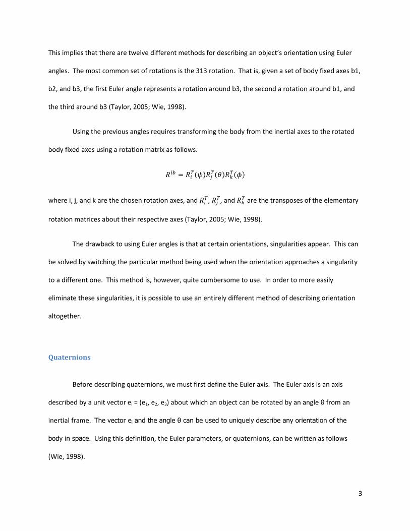
This implies that there are twelve different methods for describing an object’s orientation using Euler

angles. The most common set of rotations is the 313 rotation. That is, given a set of body fixed axes b1,

b2, and b3, the first Euler angle represents a rotation around b3, the second a rotation around b1, and

the third around b3 (Taylor, 2005; Wie, 1998).

Using the previous angles requires transforming the body from the inertial axes to the rotated

body fixed axes using a rotation matrix as follows.

�� = ��

where i, j, and k are the chosen rotation axes, and ��, ��, and �� are the transposes of the elementary

rotation matrices about their respective axes (Taylor, 2005; Wie, 1998).

The drawback to using Euler angles is that at certain orientations, singularities appear. This can

be solved by switching the particular method being used when the orientation approaches a singularity

to a different one. This method is, however, quite cumbersome to use. In order to more easily

eliminate these singularities, it is possible to use an entirely different method of describing orientation

altogether.

Quaternions

Before describing quaternions, we must first define the Euler axis. The Euler axis is an axis

described by a unit vector ei = (e1, e2, e3) about which an object can be rotated by an angle θ from an

inertial frame. The vector ei and the angle θ can be used to uniquely describe any orientation of the

body in space. Using this definition, the Euler parameters, or quaternions, can be written as follows

(Wie, 1998).

4

� = �� sin� 2⁄ �

� = �� sin� 2⁄ �

� = �� sin� 2⁄ �

� = cos� 2⁄ �

The rotation matrix is then defined as,

�� = �1 − 2� �� + �� 2� � � + � �� 2� � � − � ��2� � � − � �� 1 − 2� �� + �� 2� � � + � ��2� � � + � �� 2� � � − � �� 1 − 2� �� + ��

Using this relation, we can describe the orientation of our vehicle if we know the associated quaternions

for the vehicle’s attitude. The next step then is to solve for the quaternions.

Attitude Determination

To determine the attitude of a vehicle using an inertial system and quaternions requires that the

torques acting on the body, as well as the initial orientation and angular rates, be known. It is also

necessary to know the principle moments of inertia of the vehicle. If the moments of inertia and the

initial angular rates are known, then the angular rates at some time, t, can be determined from the

following set of equations (Wie, 1998).

� � = �!� − !�� + "�!�

� � = �!� − !�� + "�!�

5

� � = �!� − !�� + "�!�

Solving for the angular rates, the quaternions can be found using the following four equations (Wie,

1998).

� = 12 �� − �� + ��

� = 12 �� + �� − ��

� = 12 �−�� + �� + ��

� = 12 �−�� − �� − ��

This leaves us with a set of seven differential equations that need to be solved in order to calculate the

vehicle’s orientation at any given time.

6

VEHICLE STABILITY

Proper control of a vehicle requires that the vehicle be able to correct its orientation should it

encounter any disturbances that affect its intended attitude. One method for correcting attitude is

through the use of a basic quaternion feedback control system. This system can be defined as

# = −$%& − '(

where u is the torques u1, u2, and u3 applied by the actuators about the x-, y- and z-body fixed axes, ω is

the angular velocities ω1, ω2, and ω3, K and C are gain matrices, and qe is the error quaternion. qe is

defined as

� �) �) �) �)

� = � �*− �* �* �*

�* �*− �* �*

− �* �* �* �*

− �*− �*− �* �*� �

� � � ��

where q1c, q2c, q3c, and q4c are the quaternions for the desired orientation (Wie, 1998, p. 403).

All that is left to define for the control scheme are the values of K and C. Specifically, we will be

using the following three controllers:

Controller 1: $ = +, ' = -./0�1�, 1�, 1��

Controller 2: $ = �345 , ' = -./0�1�, 1�, 1��

Controller 3: $ = + 708� ��, ' = -./0�1�, 1�, 1��

Figure 2: Stability Controllers

where k, c1, c2, and c3 are constants and sgn(q4) is a function which returns 1 for positive values of q4, -1

for negative values of q4, and 0 if q4 equals zero. These controllers each work in slightly different ways,

but each brings the vehicle to the desired orientation (Wie, 1998, p. 404).

7

CHAPTER THREE: SIMULATION METHODOLOGY

MATLAB

One of the main goals of this project was to create a MATLAB simulation toolbox that could be

used to model various attitude control maneuvers. In order to do this, we needed to create function

files that were capable of modeling rigid body dynamics. The function files also needed to be able to

model torques induced by a control system.

Basic MATLAB Code Creation

For our first attempt at simulating attitude dynamics, we used Euler angles to describe the

orientation of a set of body fixed axes with respect to an inertial reference frame. We successfully

modeled drift maneuvers using this scheme, but quickly realized the limitations of using Euler angles to

describe our system. The singularities that are inherent in Euler angles severely limited the maneuvers

that we were able to model. Any time a simulation ran into one of these singularities, the program

crashed.

In order to avoid singularities, we converted our program to use quaternions instead of Euler

angles. Quaternions, unlike Euler angles, do not suffer from singularities at certain orientations. This

allowed us to simulate all of our maneuvers without having to switch between different types of Euler

rotations. The one major drawback of using quaternions is the non-intuitive way in which they describe

the orientation. It is not immediately apparent what the orientation of a vehicle is from glancing at the

quaternions unless one is proficient at reading them. The benefits of using quaternions, however, far

outweigh the drawbacks.

8

As part of the output of our simulations, we required a visual expression of the vehicle’s

rotations. To do this, we made the MATLAB code output an ellipsoid to rotate with the body fixed axes.

This ellipsoid is shaped to match the users input for the three moments of inertia of the vehicle. This

ellipsoid then rotates with the body fixed axes during the simulation.

Control Schemes

For our purposes of controlling an unmanned underwater vehicle, one basic control scheme was

required, that of stability. While in spacecraft maneuvers, various open loop controls for maneuvers

such as pointing and spin-up can be successfully implemented, the relatively large resistance caused by

water prevents such techniques from being easily used for submersibles. This can easily be shown using

a basic spin up maneuver. In space, where there is negligible resistance, a spacecraft spun up will

remain that way for a long period of time. Underwater, however, a spinning vehicle will be subjected to

the resistance of the water and the rate of spin will decrease. Because of this, we opted for closed loop

control systems. Specifically, we used feedback stability control schemes for the attitude control of our

vehicle.

In our MATLAB program, we wrote six controller function files. Three of these files are used for

basic stability with no rotation. They differ only in the actual control scheme that is implemented. The

other three are stable spin controllers, one for spin around each of the body fixed axes.

MATLAB Simulations

Once our MATLAB program was completed, we ran the code using various inputs to produce

different attitude behaviors. As a basic test of our MATLAB code, we checked to see if a well known

9

property of spinning objects held true in our simulations. That property is that an object spinning

around its major or minor axes will remain stable even with small perturbations, but that an object will

be unstable spinning around its intermediate axis (Wiesel, 1997). To test this in our simulations, we ran

the code using initial angular velocities around each of the three axes separately. We added small

torques around each of the axes to produce small perturbations. The program then outputted

quaternion plots as well as movies of the simulations.

Our last set of tests was to run the same inputs into each of the six controller function files to

see the results. The first three simulations on controllers 1, 2, and 3 will show how the different control

schemes operate in comparison to one another. The last three controllers will show how spin differs

around the body fixed x-, y-, and z-axes using a modified version of controller 3.

10

CHAPTER FOUR: EXPERIMENTAL BACKGROUND

ATTITUDE CONTROL SYSTEMS

Attitude control requires an attitude sensor system, of actuators to apply the appropriate

torques when required and a set of computational algorithms and modules to command the actuators

based on the sensor readings. The algorithms use the readings and issue the appropriate commands to

the actuators to rotate the vehicle in a given direction. The algorithms can be as simple as a

proportionality control or as complex as a nonlinear estimator. The complexity of the algorithms

depends on the particular attitude maneuver and the type of ACS device that is used.

There are currently three main types of attitude control systems being applied in current

aerospace systems. While others exist, including using electromagnets to apply torque (Sheremetevskii,

Veinberg, Vereshchagin, & Danilov-Nitusov), the three types that are most predominantly used are the

flywheel, the control moment gyroscope and stabilizing thrusters. In this section each of the three main

types will be discussed in detail, including the basic components, the advantages and disadvantages of

each and how each works from a mechanical sense.

Linear Thrusters

The first of the ACS system which will be discussed is the oldest and most common of the three,

the stabilizing thrusters. Stabilizing thrusters have been used on the majority of NASA’s manned

spacecraft including the space shuttle and the Lunar Lander. Other applications also include the ORION

satellite and both Voyagers I & II (Britannica (a)). The thrusters work on a 3-axis “reaction control”

system which means that at each point there are three thrusters (in the x-, y-, and z-directions) which

repeatedly nudge the spacecraft within the given tolerance range. Since they use such small bursts of

11

energy (in this case fuel) to keep the spacecraft in its required position, they use the smallest torque of

all the ACS systems. This translates into the least amount of strain on both the ACS hardware and the

spacecraft itself. One of the main disadvantages to using the stabilizing thrusters versus any of the

others are each thruster system is very much limited by its fuel efficiency and consumption. However,

since each thruster burn is very short and precise, a given thruster system can run off of a smaller fuel

supply for a long period of time. For example, as of April 2006, Voyagers I & II have used up a little over

half of their 100 kg fuel supply since their launch in 1977 (NASA JPL). The other main disadvantage to

using stabilizing thrusters is the thruster exhaust that is given off with each actuation. While not only

being a pollutant, the exhaust can also greatly affect the sensitive computers, sensors and optics that

many of today’s satellites, including the Hubble Telescope, have onboard. This is why many times,

aerospace engineers will choose to use flywheels, and CMGs on their more environmentally sensitive

satellites instead of using the more common stabilizing thrusters (NASA JPL).

Flywheel

While the flywheel is one of the newer technologies to be applied to attitude control systems, it

has been used in other areas for a long time. A flywheel (or momentum wheel as it is know in the

aerospace realm) is a simple device for storing momentum in a rotating mass. The simplest and most

common example of this is the potter’s wheel. They are mainly used when a given spacecraft needs to

be moved/rotated a small amount (such as keeping the Hubble Telescope pointed at a particular

star/star cluster) and when one needs to eliminate the overall mass that would be added from thruster

fuel (NASA SBIR & STTR).

The flywheel operates on a basic spin-up/spin-down movement in order to provide a means of

swapping angular momentum between spacecraft and wheels. To rotate the spacecraft a given

12

direction, the proper wheel is actuated and spins the opposite direction. To change direction/slow

down the rotation, the wheel is slowed down and spun the opposite direction. Because of this, there

are some major advantages to using momentum wheels as compared to any of the other systems (NASA

SBIR & STTR). Momentum wheels store energy more efficiently than either the CMGs or stabilizing

thrusters. Because it trades the spacecraft’s own angular momentum back and forth without the use of

any sort of fuel, it has the most precise pointing controls and for the least amount of cost, mass and

power. Those momentum wheels used for their inherent gyroscopic ability are also known as reaction

wheels or Control Moment Gyroscopes (CMGs) (NASA).

Control Moment Gyroscope

Control moment gyroscopes operate by tilting each gyro’s spin axis to apply torque. While

momentum wheels store energy more efficiently than the other ACS systems, CMGs use the power

provided more efficiently. For instance, a 100 kg CMG with a few hundred watts of power can produce

a few thousand Newton meters of torque. A momentum wheel under the same conditions would need

several megawatts of power. Because of this CMGs have been used in many of the aerospace industry’s

larger projects including Mir, Skylab and the ISS (Britannica (a)).

There are three basic types of CMG systems, single-gimbal, dual-gimbal and variable speed

gimbals. Single-gimbal CMGs are the most effective of the CMGs because it translates most if not all of

the rotor’s angular momentum directly into torque with no mechanical work being done. Because of

this, very little actual power is required (Britannica.com). This in turn allows very large torques to be

applied with minimal electrical input. The main disadvantage to the single-gimbal CMG is since only one

motor is used, a spacecraft using CMGs need at least three CMGs for a full range of motion. Even with

this, some torque may still not be useable or provide any useful motion. These “singularities,” while

13

more prevalent with the single-gimbal CMGs, exist with all three of the CMG systems. Dual-Gimbal

CMGs, while requiring more power than single-gimbal CMGs, are more versatile than the single-gimbal

because they can point the motor in any direction. Dual-gimbals are also much more efficient in storing

momentum in a mass-efficient way (Britannica (a)). This is one of the reasons dual-gimbal CMGs are

currently being used on board the ISS. The only disadvantage to dual-gimbal CMGs besides the

singularities that exist with all CMG types is the excessive power demands because one actuation by one

of the gimbals often requires an opposite reactive actuation by the other gimbal.

The third and final of the CMG systems is the variable-speed CMG. While still in the design

phase of production, the variable-speed CMG is showing it can deliver a torque magnitude that is

smaller than those of normal gimbal motion and therefore require less power (Britannica (a)). They

work by using spin up and spin down maneuvers, similar to those used in flywheels, to operate the

gimbal motors (Moore, 2003). The only disadvantages that have been observed thus far are the same

singularities that are existent in all CMG systems.

14

VEHICLE COMPONENTS

The following is a list with descriptions of the components we purchased and used for our test

vehicle.

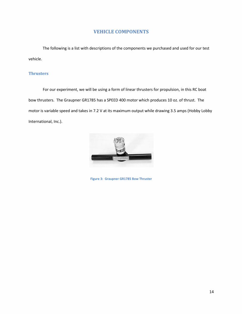
Thrusters

For our experiment, we will be using a form of linear thrusters for propulsion, in this RC boat

bow thrusters. The Graupner GR1785 has a SPEED 400 motor which produces 10 oz. of thrust. The

motor is variable speed and takes in 7.2 V at its maximum output while drawing 3.5 amps (Hobby Lobby

International, Inc.).

Figure 3: Graupner GR1785 Bow Thruster

15

Sun SPOT

For our vehicle, we needed onboard micro-controllers to run the processing of sensor inputs

and thruster outputs. For this purpose, we purchased Sun SPOTs. Sun SPOTs, as shown in Figure 4, are

small Java based controllers. They come with an array of features that include a three axis

accelerometer, temperature sensor, eight LEDs, light sensor, as well as a wireless receiver. The wireless

receiver can be used to communicate with other Sun SPOTs and a base station connected to a computer

(Sun Microsystems, 2008). For our vehicle, we will be using the accelerometers to identify the direction

of the Earth. The temperature sensor will be used to monitor that the inside of the vehicle stays within

reasonable temperatures. The wireless receiver will be used to communicate with a computer and

other Sun SPOTs.

Figure 4: Sun SPOT

16

Battery Pack

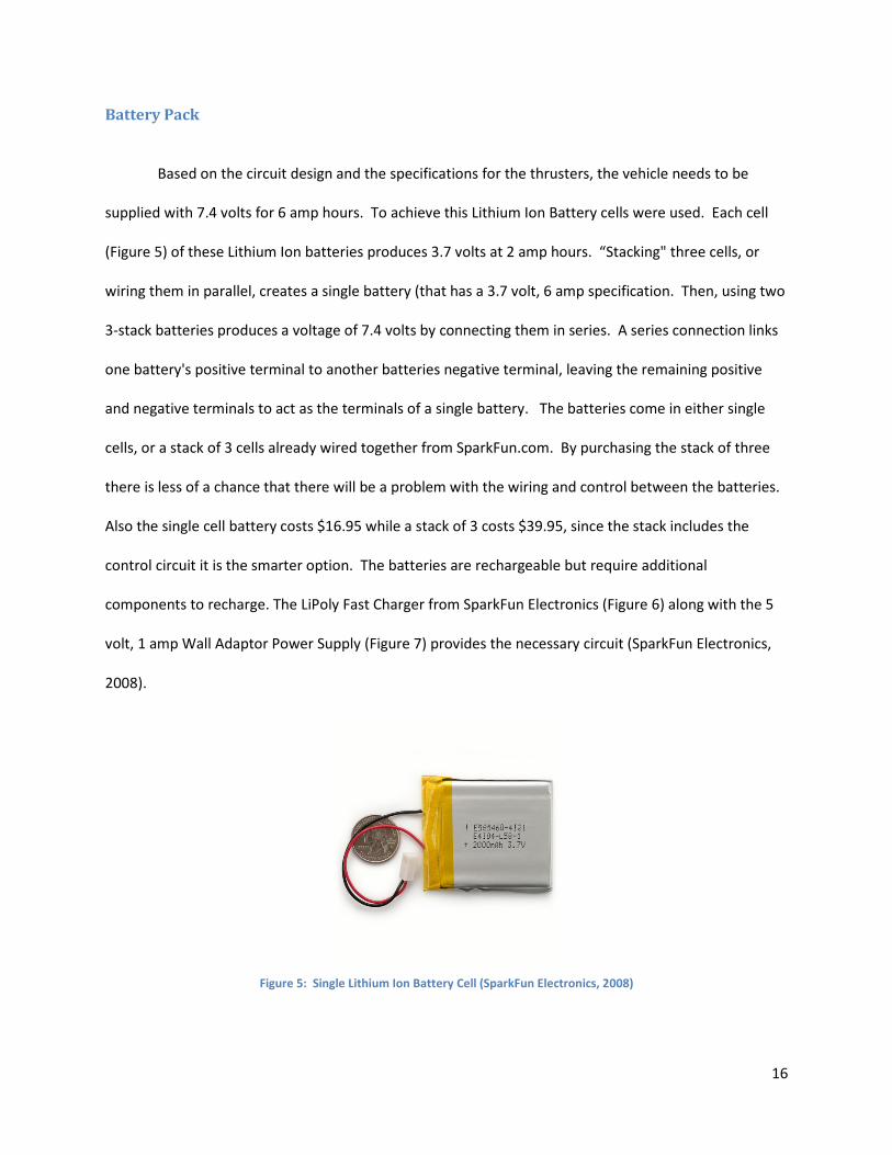
Based on the circuit design and the specifications for the thrusters, the vehicle needs to be

supplied with 7.4 volts for 6 amp hours. To achieve this Lithium Ion Battery cells were used. Each cell

(Figure 5) of these Lithium Ion batteries produces 3.7 volts at 2 amp hours. “Stacking" three cells, or

wiring them in parallel, creates a single battery (that has a 3.7 volt, 6 amp specification. Then, using two

3-stack batteries produces a voltage of 7.4 volts by connecting them in series. A series connection links

one battery's positive terminal to another batteries negative terminal, leaving the remaining positive

and negative terminals to act as the terminals of a single battery. The batteries come in either single

cells, or a stack of 3 cells already wired together from SparkFun.com. By purchasing the stack of three

there is less of a chance that there will be a problem with the wiring and control between the batteries.

Also the single cell battery costs $16.95 while a stack of 3 costs $39.95, since the stack includes the

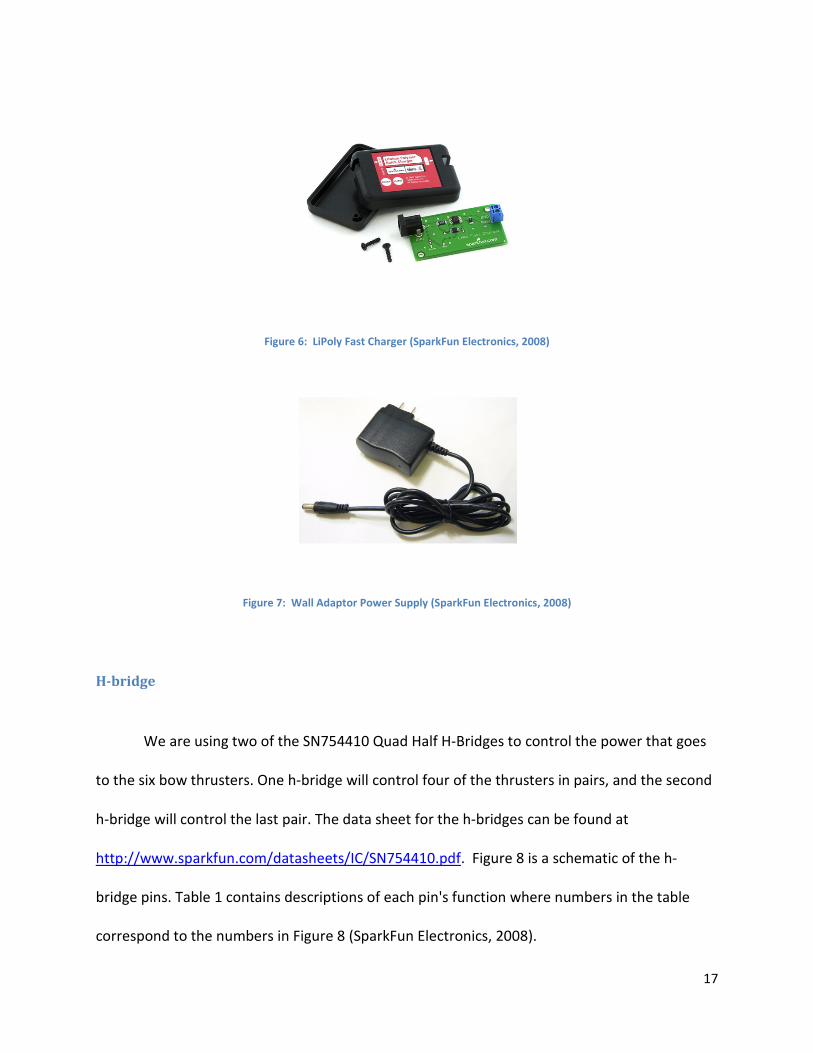
control circuit it is the smarter option. The batteries are rechargeable but require additional

components to recharge. The LiPoly Fast Charger from SparkFun Electronics (Figure 6) along with the 5

volt, 1 amp Wall Adaptor Power Supply (Figure 7) provides the necessary circuit (SparkFun Electronics,

2008).

Figure 5: Single Lithium Ion Battery Cell (SparkFun Electronics, 2008)

17

Figure 6: LiPoly Fast Charger (SparkFun Electronics, 2008)

Figure 7: Wall Adaptor Power Supply (SparkFun Electronics, 2008)

H-bridge

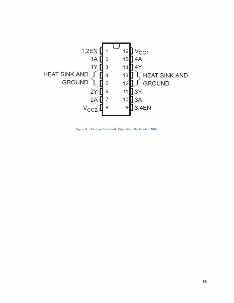
We are using two of the SN754410 Quad Half H-Bridges to control the power that goes

to the six bow thrusters. One h-bridge will control four of the thrusters in pairs, and the second

h-bridge will control the last pair. The data sheet for the h-bridges can be found at

http://www.sparkfun.com/datasheets/IC/SN754410.pdf. Figure 8 is a schematic of the h-

bridge pins. Table 1 contains descriptions of each pin's function where numbers in the table

correspond to the numbers in Figure 8 (SparkFun Electronics, 2008).

18

Figure 8: H-bridge Schematic (SparkFun Electronics, 2008)

19

Table 1: Pin Functions

Pin Functions

Pin Label Function

1 1,2EN 1, 2 enable, if there is power to this pin, pins 2, 3, 6, and 7 may

operate.

2 1A Control for Motor Pair 1

3 1Y Power out to Motor Pair 1

4 Heat Sink and Ground Provide a ground for the circuits and a heat sink if needed.




8 Vcc2 Input pin of power for Motors

9 3,4EN 3, 4 enable, if there is power to this pin, pins 10, 11, 14, and 15 may

operate.







16 Vcc1 Power input for the chip, provides power needed for functions.

The most fundamental operation of this chip is the two enable pins, 1 and 9. When these two

pins don't have power, the chip will not provide any power to either motor pair. A switch can be used to

provide an emergency off resort if required. When the enable pins are powered, the power to Vcc1

provides the next determining factor. When pin 2, 1A, is at an equivalent voltage to pin 1, 1,2EN, pin 2 is

considered to be "high". In conjunction, when pin 2 has a voltage unequal to pin 1, pin 2 is considered

"low". This is also the operation of pin 7, 2A, working with pin 1, and pins 10 and 15, 3A and 4A,

respectively, working with pin 9, EN3,4. Pins 2 and 7 provide the logic to drive a motor, or if the motors

work in conjunction, as is our case, they will provide the same logic for a motor pair through circuit work

later in the process. The logic behind a pin pair is the direction of power through the circuit. When pin 2

is "high" and pin 7 is "low" the power will flow from pin 3, 1Y, to pin 6 2Y, this will be nominally called a

"forward" flow. Conversely when pin 2 is "low" and pin 7 is "high" the power will flow from pin 6 to pin

20

3, nominally a "reverse" flow. If both pin 2 and pin 7 are "low" there will be no power flowing from pin 3

or pin 7, which results in the motors not being powered on. The programming used on the Sun SPOT

micro controllers does not permit both pin 2 and pin 7 to both be "high". The pin pairs that operate in

the manner detailed and the possible power flows are in the table below. Pin 8 Vcc2 is the input power

that will flow out of pins 3, 6, 11, and 14. This means the power supplied to pin 8 will be the power that

flows out of one of the four pins with a Y label corresponding to the same numbered pin with an A label

(SparkFun Electronics, 2008).

Table 2: Power Flow

Power Flow

1,2EN pin 2 (1A) pin 7, (2A) Direction of Flow

High High Low Forward pin 3 (1Y) to pin 6 (2Y)

High Low High Reverse pin 6 (2Y) to pin 3 (1Y)

High Low Low No Flow

Low High Low Not On

Low Low High Not On

Low Low Low Not On

3,4EN pin 10 (3A) pin 14, (4A) Direction of Flow

High High Low Forward pin 10 (3Y) to pin 14 (4Y)

High Low High Reverse pin 14 (4Y) to pin 10 (3Y)

High Low Low No Flow

Low High Low Not On

Low High Low Not On

Low Low Low Not On

21

Breadboard

For our purposes, a simple breadboard is necessary. The small, self-adhesive breadboards will

fit the necessary circuit components and is small enough to fit inside the vehicle (SparkFun Electronics,

2008).

Figure 9: Small Self-Adhesive Breadboard (SparkFun Electronics, 2008)

22

ADIS Gyroscope

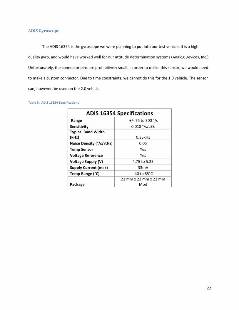
The ADIS 16354 is the gyroscope we were planning to put into our test vehicle. It is a high

quality gyro, and would have worked well for our attitude determination systems (Analog Devices, Inc.).

Unfortunately, the connector pins are prohibitively small. In order to utilize this sensor, we would need

to make a custom connector. Due to time constraints, we cannot do this for the 1.0 vehicle. The sensor

can, however, be used on the 2.0 vehicle.

Table 3: ADIS 16354 Specifications

ADIS 16354 Specifications Range +/- 75 to 300 °/s

Sensitivity 0.018 °/s/LSB

Typical Band Width

(kHz) 0.35kHz

Noise Density (°/s/rtHz) 0.05

Temp Sensor Yes

Voltage Reference Yes

Voltage Supply (V) 4.75 to 5.25

Supply Current (max) 33mA

Temp Range (°C) -40 to 85°C

Package

23 mm x 23 mm x 23 mm

Mod

23

WATERPROOFING

Waterproofing, in the basic sense, is the process applied to any surface or material in order to

prevent the passage of water and/or water vapor. This process normally involves the application of

membranous materials to the area designated to be waterproofed. These materials include but are not

limited to wax and resin mixtures, aluminum salts, silicates, PVC, fluoro-chemicals, paraffin, bituminous

materials and drying oils. The most commonly used waterproofing materials are caulk, hot glue,

waterproofing grease and spray-on silicates (Britannica (b)).

For our experiment, we initially tried using waterproof grease for our motors. Unfortunately,

we discovered that the grease not only didn’t work and allowed water through, causing our engine to

rust and seize, but also created quite a mess out of the thruster tubing and motor. This obviously

removed this option from the list of possible waterproofing agents. The test vehicle itself is put

together with hot glue. When we water tested the vehicle initially, we noted a few holes in the vessel.

All of these holes were patched with a second and third coating of hot glue, making the vehicle (without

any holes drilled for the thrusters) completely water tight.

When it comes to waterproofing the holes for the thruster tubing, we encountered some

problems. The caulk we were using was, from all accounts, not keeping water out of the test container.

We found a few potential holes which we tried applying a second coat of caulk to which at this point,

have yet to retest. From all accounts, it appears as though we will probably not be using the caulk for

the area around the holes, and will instead most likely use hot glue to seal the holes as it has done

magnificently for us with the test vehicle. The only problem with using the hot glue instead of the caulk

will be in applying it to the underside of the tubing, a job that was made easier by the caulks extended

drying time versus that of the hot glue.

24

CHAPTER FIVE: EXPERIMENTAL METHODOLOGY

BOW THRUSTER TESTING

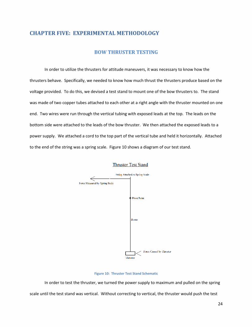
In order to utilize the thrusters for attitude maneuvers, it was necessary to know how the

thrusters behave. Specifically, we needed to know how much thrust the thrusters produce based on the

voltage provided. To do this, we devised a test stand to mount one of the bow thrusters to. The stand

was made of two copper tubes attached to each other at a right angle with the thruster mounted on one

end. Two wires were run through the vertical tubing with exposed leads at the top. The leads on the

bottom side were attached to the leads of the bow thruster. We then attached the exposed leads to a

power supply. We attached a cord to the top part of the vertical tube and held it horizontally. Attached

to the end of the string was a spring scale. Figure 10 shows a diagram of our test stand.

Figure 10: Thruster Test Stand Schematic

In order to test the thruster, we turned the power supply to maximum and pulled on the spring

scale until the test stand was vertical. Without correcting to vertical, the thruster would push the test

25

stand to an angle off of vertical and the weight of the thruster and test stand would begin to influence

the readings. With the test stand vertical, we recorded the reading on the spring scale. We then

continued to lower the voltage on the power supply by increments of 0.2 volts at a time and repeated

the procedure to get spring scale measurements for each voltage. We continued recording readings

until the difference between subsequent readings became negligible. At this point, error introduced by

friction in the test stand, torque caused by the wire, and other errors prevent accurate readings of the

thrust. We then repeated this procedure two more times to get three sets of data.

Analyzing the results requires converting the force measured by the spring scale readings to the

thrust provided by the thruster. This is simply done by converting the readings to the torque on the test

stand and then converting back to force at the distance of the thruster from the pivot point. We then

tabulated the data and averaged the results of the three tests. Finally, we graphed the average thrusts

to get the thrust vs. voltage curve in Figure 24.

26

VEHICLE CONSTRUCTION

Our Project had a variety of requirements for the vehicle body. These requirements were to

provide a water tight container for the internal components of the system, to have an access point

through which the internal components could be reached, and be spacious enough to hold all the

necessary components. Two other goals we had for the vehicle, that were not necessarily required but

were preferable, were to have the vehicle body be symmetric around all three axis of rotation, and to be

buoyant.

The first solutions we developed all were less than satisfactory for a variety of reasons. We first

thought to manufacture a body from aluminum in the WPI machine shops. To do this would have

allowed us practically any shape we desired however there were some drawbacks. The first is the

difficulty of implementing a water tight seal on a metal, machined body. The relative difficulty of

construction, probable weight of the aluminum body, possible failures with water tightness, and

expenses made this not an ideal method. The second idea we had was to purchase a container that was

about 6 inches on each side, which also had a water tight seal around the opening. Even with our

extensive search we were unable to find a container that met our specifications. The only containers

that we found were either not the correct dimensions or did not have a water tight seal. This led to our

decision that the purchase of a premade container was also out of the question for our purposes.

The solution that we came to in order to meet these requirements was reached by thinking

outside the box and creatively. We decided to manufacture our own vehicle body; however we decided

to assemble containers that would be otherwise unsuitable in meeting the above requirements. We

decided upon plastic containers with watertight lids. We saw that when six of these containers were

assembled edge to edge they would form a cube with distended sides. This configuration provided an

extra space for components to fit inside the vehicle. The use of plastic containers also has the added

27

benefit of a light weight body, which is very buoyant. Figure 11 shows the vehicle body with the

thrusters mounted inside.

Figure 11: Vehicle Body with Thrusters

The largest obstacles we faced with the plastic containers were the water tight seals between

containers and the access to the inside of the vehicle. The solution we developed to the problem with

watertight seals was to use hot glue between the containers edges. The hot glue not only provides a

rigid bond between containers but also bonds to the plastic containers and seals the gaps completely.

This left the additional problem of access into the components inside the vehicle, since the hot glue as

stated would bond and seal the containers together. The most reasonable solution to this problem was

to not glue two of the containers to the vehicle body but to glue two of the covers in place of the

containers. This allowed for the containers to be attached and detached from the covers while

maintaining a watertight seal. Figure 12 shows the vehicle body with one container detached.

28

Figure 12: Vehicle Body with One Side Open

Before we attached the covers to the vehicle we removed the majority of the centers of the covers to

provide access to the inside components. One added benefit of having two removable sections for

access is that they are located opposite each other on the vehicle, which keeps the center of mass

located in the middle of the vehicle, leading to easier control schemes.

The other challenge with water tightness is the thruster attachment. The ends of the tubes of

the thruster must be exposed to the water, however there needs to be a water tight seal between the

thruster tube and the vehicle, as well as on the joint of the tubes with the main thruster component. To

ensure a seal in these areas, waterproof caulk was purchased and used.

29

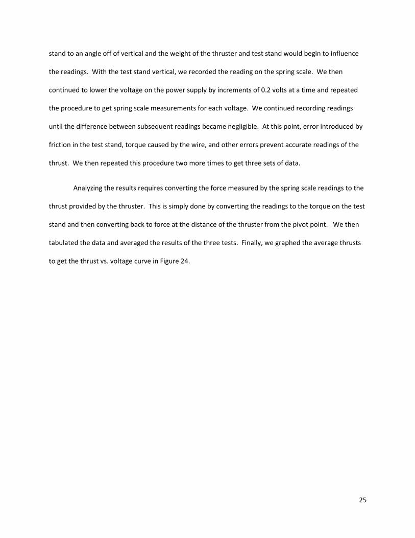
CIRCUIT DESIGN

The circuit design inside the vehicle is fairly simple and straightforward. The system consists of

5 major components, the thrusters, batteries, micro controllers, sensors and h-bridges. The thrusters,

batteries and sensors are discussed in more detail in separate sections. The micro controllers and the h-

bridges are the primary components of the electric circuit.

The micro controller is the computing center of the system. This device takes the sensor

outputs and calculates the necessary power needed at each thruster based on our control schemes and

thrust curves. This information is then transmitted through the h-bridges. The micro controller also has

a wireless transmitter, and can be programmed to talk to another micro controller that can be

connected to a computer via an USB cable. This allows for the computer to do the heavier math

calculations if desired, or the computer can just take the data output by the first micro controller and

use that information to determine the correct thrust needed for stability, and relay that information

back to the vehicle through the micro controllers.

The h-bridge acts as a relay between the batteries and the thrusters and the micro controller

and the thrusters. Each h-bridge can act as a relay for up to four thrusters. For our system however one

h-bridge only needs to control two thrusters while the other h-bridge controls the other four. The h-

bridge also controls the power supplied to each thruster. It ensures that the battery is supplying the

correct power to the thruster as dictated by the micro controller.

30

Figure 13: Circuit Design

31

CHAPTER SIX: SIMULATION RESULTS AND ANALYSIS

MATLAB RESULTS

Our MATLAB program was required to be able to simulate rigid body dynamics as well as some

basic control schemes to control the attitude of a simulated vehicle. As outputs, our program created

quaternion plots to describe orientation as well as movies of our simulations. Figure 14 shows one

frame of a simulation.

Figure 14: Simulation Movie Frame

Free Rotation Stability Testing

As mentioned in the methodology, we ran three separate simulations to test the stability of an

object rotating about its major, minor, and intermediate axes. For these simulations we used J1, J2, and

J3 equal to 150, 145, and 60 respectively. The initial quaternions q1, q2, q3, and q4 were set to 0, 0, 0, and

32

1. The external torque around each axis was set to be 0.1. Figure 15 shows a plot with an initial angular

rate of 0.5 around the major axis. The effects of the perturbations can most easily be seen by the slight

variations in the red and black lines. On the whole, however, the plot shows quite stable rotation.

Figure 15: Free Spin About Major Axis

Figure 16 shows the behavior when the initial angular velocity around the minor axis is set to

0.5. The fluctuations in this plot are larger than in the previous as is to be expected from spin around

the minor axis compared to the major. While there is some wobble, however, the rotation is still stable.

33

Figure 16: Free Spin About Minor Axis

Figure 17 shows the object’s behavior when the initial angular velocity around the intermediate

axis is set to 0.5. This plot clearly shows significant deviation from stable spin. These results fall directly

in line with the type of behavior we expected.

Figure 17: Free Spin About Intermediate Axis

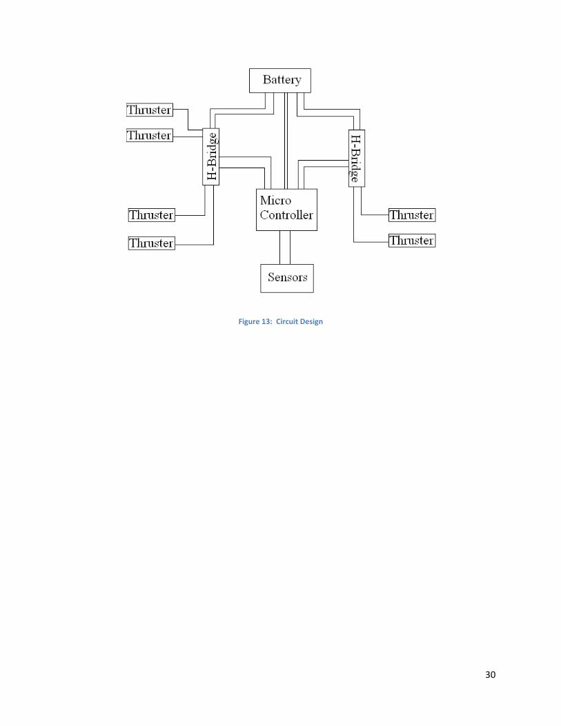
Our second set of tests was simply running each of the six controllers using the same inputs. For

these tests, we used J1, J2, and J3 equal to 15, 14.5, and 6 respectively. The initial quaternions q1, q2, q3,

34

and q4 were set to 0, 0, 0, and 1. The desired quaternions q1c, q2c, q3c, and q4c were set to 0.5, -0.5, 0.5,

and 0.5. The controller constants k, c1, c2, c3 were set to 1, 4, 4, and 4. Initial angular velocities and

initial torques were all set to 0.

Comparing the first three plots, the stationary stability controller plots, suggests that controllers

1 and 3 act in a similar fashion. Both plots follow a remarkably similar path. They both also take around

37 seconds to converge with the given inputs. Controller 2 has a different shape with more erratic

movements. This controller, however, converges around 26 seconds. This controller is more aggressive

and tends to converge faster than the other two controllers.

Figure 18: Controller 1

35



36

The following three plots are of controllers 4, 5, and 6, the stable spin controllers. They each act

roughly the same as they were derived from the same stationary stability controller. Controller 4

appears to act more erratically, but this is likely an artifact of the initial conditions.



37


38

CHAPTER SEVEN: EXPERIMENTAL RESULTS AND ANALYSIS

BOW THRUSTER TEST RESULTS

As mentioned earlier, in order for us to be able to properly control our underwater vehicle’s

attitude, we needed to know the behavior of the thrusters. Specifically, we needed to know the thrust

that each thruster produced when supplied with varying voltages. Below is a table of our collected data

for the bow thruster test. The test columns are the recorded force values from our spring scale. The

force column is the calculated force provided by the bow thrusters. The forces found during these tests

are likely to be lower than the forces we will achieve on the actual vehicle. This is due to losses in the

wire we used to connect the power supply to the thruster. The wire we used was 25 feet long, whereas

the wiring in the test vehicle will be much shorter.

Table 4: Bow Thruster Thrust vs. Voltage

Thrust vs. Voltage

Voltage test 1 test 2 test 3 Average Force (N)

1.4 3.2 2.8 2.8 2.9 0.453

1.6 3.2 2.8 3.0 3.0 0.463

1.8 3.6 3.4 3.6 3.5 0.545

2.0 4.0 3.8 4.0 3.9 0.607

2.2 4.4 4.0 4.4 4.3 0.658

2.4 4.8 4.4 4.8 4.7 0.720

2.6 5.2 4.5 5.6 5.1 0.787

2.8 6.0 5.0 6.0 5.7 0.875

3.0 6.2 5.6 6.4 6.1 0.936

3.2 6.8 6.8 7.2 6.9 1.070

3.4 7.2 7.0 8.0 7.4 1.142

3.6 8.0 7.7 8.4 8.0 1.240

3.8 8.4 8.2 8.8 8.5 1.307

4.0 8.8 8.2 9.2 8.7 1.348

4.2 9.2 8.8 9.6 9.2 1.420

39

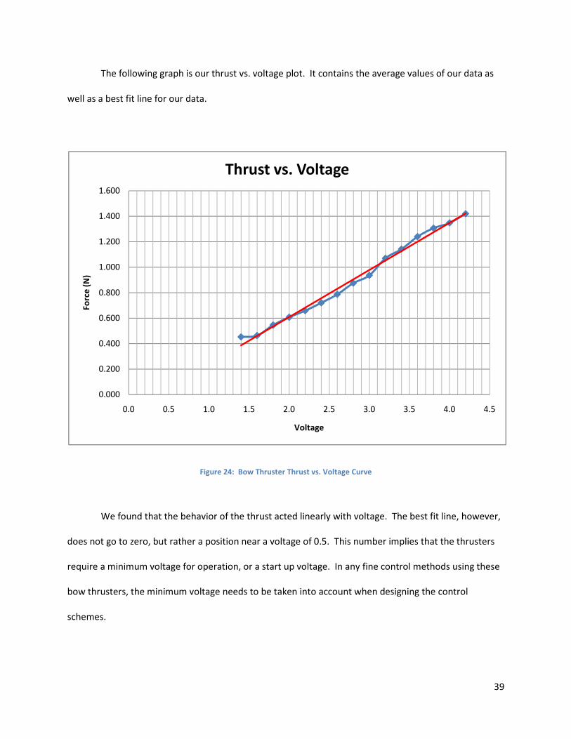
The following graph is our thrust vs. voltage plot. It contains the average values of our data as

well as a best fit line for our data.

Figure 24: Bow Thruster Thrust vs. Voltage Curve

We found that the behavior of the thrust acted linearly with voltage. The best fit line, however,

does not go to zero, but rather a position near a voltage of 0.5. This number implies that the thrusters

require a minimum voltage for operation, or a start up voltage. In any fine control methods using these

bow thrusters, the minimum voltage needs to be taken into account when designing the control

schemes.

0.000

0.200

0.400

0.600

0.800

1.000

1.200

1.400

1.600

0.0 0.5 1.0 1.5 2.0 2.5 3.0 3.5 4.0 4.5

Fo

rce

(N

)

Voltage

Thrust vs. Voltage

40

CHAPTER EIGHT: RECOMMENDATIONS AND CONCLUSIONS

SIMULATION

As this MQP is the beginning of a larger research project, we recommend that future groups use

and modify our MATLAB code, found in APPENDIX A: MATLAB CODE, to work with their systems. We

also recommend that the MATLAB code be updated to be more robust in what it is capable of

simulating. Specifically, an environmental simulator could be added in order to mimic various

conditions. As it stands, the code has no way of adding random torques to the simulation to mimic

perturbations caused by disturbances such as water currents or micro-collisions. These types of random

perturbations would be useful in studying the stability control schemes found in the MATLAB code. We

also recommend that the program include more control schemes in order to simulate different

maneuvers such as spin up, spin down, or bang-bang maneuvers. The current code only has closed loop

feedback stability controllers. It does not have any of the open loop controllers mentioned.

41

VEHICLE CONSTRUCTION

During this project, we attempted to build an autonomous underwater vehicle capable of

controlling its orientation. Unfortunately, due to setbacks, we were unable to complete the vehicle. As

such, our first recommendation concerning the vehicle is to complete its construction. This includes

setting up the circuits with the breadboards, h-bridges, Sun SPOTs, batteries, and motors to work

together. We also recommend that the java code, found in APPENDIX B: SUN SPOT SAMPLE CODE, be

modified to work with the h-bridges and motors. The system will need extensive testing in order to

ensure that it works in the intended fashion.

Through our research and testing, we’ve concluded a few things concerning the larger vehicle

that Professor Hussein is planning on building. The first is that it will need more powerful thrusters than

the ones used on our test vehicle. Our bow thruster testing proved that while the bow thrusters are

useable in controlling the orientation of our small test vehicle, they will not be powerful enough to both

correct the attitude of the larger vehicle as well as control its translational movement with satisfactory

results.

In our research into batteries for our test vehicle we looked at NiCad and lithium-ion batteries.

We found that lithium-ion batteries were superior in their power to weight ratio, ability to charge and

discharge, and overall size. We recommend using lithium-ion batteries in the larger test vehicle in order

to save space, weight, and have higher power batteries than NiCad.

In order for our vehicle to remain underwater while not resting on the bottom of the tank, we

designed it to be neutrally buoyant. While on a simple small scale test vehicle this might be acceptable,

this is not ideal for a larger autonomous vehicle. The larger vehicle must be able to change its depth at

42

will. We recommend the use of a ballast tank or multiple ballast tanks to allow for this versatility. This

would allow the vehicle to be a more useful test platform.

Because the ADIS Gyroscope purchased for our project was both difficult to use and highly

expensive, we did not incorporate it into our test vehicle. Unfortunately, this left us with only the

onboard accelerometers of the Sun SPOTs. While these are useful for finding the direction of the Earth,

and can therefore be used to level the vehicle, they do not describe orientation about the z-axis, or the

axis pointing away from the Earth. This makes it impossible to determine direction with the Sun SPOT

accelerometers alone. For this reason, we recommend that the ADIS Gyroscope purchased for our

project be used in the larger test vehicle for the purpose of attitude determination.

43

APPENDIX A: MATLAB CODE

The following code is the MATLAB program created for this project. Main.m is the initializing

program where all of the variables are set. Point.m is the code that runs each of the controllers, creates

the ellipsoid, runs the simulation movie, and outputs the quaternion plots. Controllers 1, 2, and 3

correspond to the controllers in Figure 2 on page 6. Controllers 4, 5, and 6 are modified versions of

controller 3 to create stable spin around the body fixed x-, y-, and z-axes respectively.

Main.m

global J1 J2 J3 q1c q2c q3c q4c k c1 c2 c3 ue1 ue2 ue3;

% Time t=0:.3:50;

% Moments of Inertia J1=15; J2=14.5; J3=6;

% Desired Quaternions q1c=.5; q2c=-.5; q3c=.5; q4c=.5;

% Controller Constants k=1; c1=4; c2=4; c3=4;

% Initial Quaternions q1=0; q2=0; q3=0; q4=1;

% Initial Omegas omega1=0; omega2=0; omega3=0;

%External torques ue1=0;

44

ue2=0; ue3=0;

% Controller 1, 2, 3, 4, 5, or 6 controller=3;

% Performs the calculations y0=[q1 q2 q3 q4 omega1 omega2 omega3]; [T,y] = point(t,y0,controller);

45

Point.m

function [T,y] = point(t,y0,controller)

global u1 u2 u3 J1 J2 J3;

% Initial Control Torques u1=0; u2=0; u3=0;

% Calls one of the controller functions options = odeset('RelTol',1e-5,'AbsTol',1e-5); if controller==6 [T,y] = ode45(@controller6,t,y0,options); elseif controller==5 [T,y] = ode45(@controller5,t,y0,options); elseif controller==4 [T,y] = ode45(@controller4,t,y0,options); elseif controller==3 [T,y] = ode45(@controller3,t,y0,options); elseif controller==2 [T,y] = ode45(@controller2,t,y0,options); else [T,y] = ode45(@controller1,t,y0,options); end

% Plots Euler Angles figure(1) hold off plot(T,y(:,1),'-black') hold on figure(1) plot(T,y(:,2),'-red') hold on figure(1) plot(T,y(:,3),'-blue') hold on figure(1) plot(T,y(:,4),'-green') hold on grid xlabel('time, seconds') ylabel('q1 (black), q2 (red), q3 (blue), q4 (green)') title('Quaternion Plots')

% Defines identity matrix i1=[1 0 0]'; i2=[0 1 0]'; i3=[0 0 1]';

% Ellipsoid *********************************** E1(1)=((J2+J3-J1)/2)^.5; E1(2)=((J1-J2+J3)/2)^.5;

46

E1(3)=((J1+J2-J3)/2)^.5; E2=E1(1);

if E2<E1(2) E2=E1(2); end if E2<E1(3) E2=E1(3); end

E2=1/(E2*1.25); E1=E2*E1;

edef=25; edef2=edef+1; [xe1, ye1, ze1] = ellipsoid(0,0,0,E1(1),E1(2),E1(3),edef); % End Ellipsoid *******************************

% For loop runs MatLab movie for ii=1:length(t),

% Defines Rotation Matrix R(:,:,ii)=[1-2*(y(ii,2)^2+y(ii,3)^2) 2*(y(ii,1)*y(ii,2)+y(ii,3)*y(ii,4))

2*(y(ii,1)*y(ii,3)-y(ii,2)*y(ii,4)) ; 2*(y(ii,2)*y(ii,1)-y(ii,3)*y(ii,4)) 1-

2*(y(ii,1)^2+y(ii,3)^2) 2*(y(ii,2)*y(ii,3)+y(ii,1)*y(ii,4)) ;

2*(y(ii,3)*y(ii,1)+y(ii,2)*y(ii,4)) 2*(y(ii,3)*y(ii,2)-y(ii,1)*y(ii,4)) 1-

2*(y(ii,1)^2+y(ii,2)^2)];

% Defines body fixed axis b1=R(:,:,ii)*i1; b2=R(:,:,ii)*i2; b3=R(:,:,ii)*i3;

% Rotates the ellipsoid ************************ xe2=zeros(edef2,edef2); ye2=zeros(edef2,edef2); ze2=zeros(edef2,edef2);

for jj=1:edef2, for kk=1:edef2, ll=[xe1(jj,kk) ye1(jj,kk) ze1(jj,kk)]'; mm=R(:,:,ii)*ll; xe2(jj,kk)=mm(1); ye2(jj,kk)=mm(2); ze2(jj,kk)=mm(3); end end % End ellipsoid rotation ***********************

% Plots MatLab movie figure(3)

47

plot3([0 i1(1)],[0 i1(2)],[0 i1(3)],'-black','LineWidth',2) hold on plot3([0 i2(1)],[0 i2(2)],[0 i2(3)],'-black','LineWidth',2) hold on plot3([0 i3(1)],[0 i3(2)],[0 i3(3)],'-black','LineWidth',2) hold on

plot3([0 -i1(1)],[0 -i1(2)],[0 -i1(3)],'-yellow','LineWidth',2) hold on plot3([0 -i2(1)],[0 -i2(2)],[0 -i2(3)],'-yellow','LineWidth',2) hold on plot3([0 -i3(1)],[0 -i3(2)],[0 -i3(3)],'-yellow','LineWidth',2) hold on

plot3([0 b1(1)],[0 b1(2)],[0 b1(3)],'-r','LineWidth',2) hold on plot3([0 b2(1)],[0 b2(2)],[0 b2(3)],'-g','LineWidth',2) hold on plot3([0 b3(1)],[0 b3(2)],[0 b3(3)],'-b','LineWidth',2) hold on grid xlabel('i_1') ylabel('i_2') zlabel('i_3') az = 135; el = 45; view(az, el); surfl(xe2, ye2, ze2) colormap copper hold off axis equal length(t)

end

48

Controller1.m

function dy = controller1(t,y)

global u1 u2 u3 ue1 ue2 ue3 J1 J2 J3 q1c q2c q3c q4c k c1 c2 c3;

dy = zeros(7,1); % a column vector

% Quaternions

dy(1)=((y(7)*y(2)-y(6)*y(3)+y(5)*y(4))*.5);

dy(2)=((-y(7)*y(1)+y(5)*y(3)+y(6)*y(4))*.5);

dy(3)=((y(6)*y(1)-y(5)*y(2)+y(7)*y(4))*.5);

dy(4)=((-y(5)*y(1)-y(6)*y(2)-y(7)*y(3))*.5);

% Omegas

dy(5)=(u1+ue1+(J2-J3)*y(6)*y(7))/J1;

dy(6)=(u2+ue2+(J3-J1)*y(7)*y(5))/J2;

dy(7)=(u3+ue3+(J1-J2)*y(5)*y(6))/J3;

% Error Quaternions

qe1=(q4c*y(1)+q3c*y(2)-q2c*y(3)-q1c*y(4));

qe2=(-q3c*y(1)+q4c*y(2)+q1c*y(3)-q2c*y(4));

qe3=(q2c*y(1)-q1c*y(2)+q4c*y(3)-q3c*y(4));

% Control Torques

u1=-k*qe1-c1*y(5);

u2=-k*qe2-c2*y(6);

u3=-k*qe3-c3*y(7);

49

Controller2.m




% Quaternions

dy(1)=((y(7)*y(2)-y(6)*y(3)+y(5)*y(4))*.5);

dy(2)=((-y(7)*y(1)+y(5)*y(3)+y(6)*y(4))*.5);

dy(3)=((y(6)*y(1)-y(5)*y(2)+y(7)*y(4))*.5);

dy(4)=((-y(5)*y(1)-y(6)*y(2)-y(7)*y(3))*.5);

% Omegas

dy(5)=(u1+ue1+(J2-J3)*y(6)*y(7))/J1;

dy(6)=(u2+ue2+(J3-J1)*y(7)*y(5))/J2;

dy(7)=(u3+ue3+(J1-J2)*y(5)*y(6))/J3;

% Error Quaternions

qe1=(q4c*y(1)+q3c*y(2)-q2c*y(3)-q1c*y(4));

qe2=(-q3c*y(1)+q4c*y(2)+q1c*y(3)-q2c*y(4));

qe3=(q2c*y(1)-q1c*y(2)+q4c*y(3)-q3c*y(4));

qe4=(q1c*y(1)+q2c*y(2)+q3c*y(3)+q4c*y(4));

% Control Torques

u1=-(k/qe4^4)*qe1-c1*y(5);

u2=-(k/qe4^4)*qe2-c2*y(6);

u3=-(k/qe4^4)*qe3-c3*y(7);

50

Controller3.m




% Quaternions

dy(1)=((y(7)*y(2)-y(6)*y(3)+y(5)*y(4))*.5);

dy(2)=((-y(7)*y(1)+y(5)*y(3)+y(6)*y(4))*.5);

dy(3)=((y(6)*y(1)-y(5)*y(2)+y(7)*y(4))*.5);

dy(4)=((-y(5)*y(1)-y(6)*y(2)-y(7)*y(3))*.5);

% Omegas

dy(5)=(u1+ue1+(J2-J3)*y(6)*y(7))/J1;

dy(6)=(u2+ue2+(J3-J1)*y(7)*y(5))/J2;

dy(7)=(u3+ue3+(J1-J2)*y(5)*y(6))/J3;

% Error Quaternions

qe1=(q4c*y(1)+q3c*y(2)-q2c*y(3)-q1c*y(4));

qe2=(-q3c*y(1)+q4c*y(2)+q1c*y(3)-q2c*y(4));

qe3=(q2c*y(1)-q1c*y(2)+q4c*y(3)-q3c*y(4));

qe4=(q1c*y(1)+q2c*y(2)+q3c*y(3)+q4c*y(4));

% Control Torques

u1=-(k*sign(qe4))*qe1-c1*y(5);



51

Controller4.m




% Quaternions

dy(1)=((y(7)*y(2)-y(6)*y(3)+y(5)*y(4))*.5);

dy(2)=((-y(7)*y(1)+y(5)*y(3)+y(6)*y(4))*.5);

dy(3)=((y(6)*y(1)-y(5)*y(2)+y(7)*y(4))*.5);

dy(4)=((-y(5)*y(1)-y(6)*y(2)-y(7)*y(3))*.5);

% Omegas

dy(5)=(u1+ue1+(J2-J3)*y(6)*y(7))/J1;

dy(6)=(u2+ue2+(J3-J1)*y(7)*y(5))/J2;

dy(7)=(u3+ue3+(J1-J2)*y(5)*y(6))/J3;

% Error Quaternions

qe1=(q4c*y(1)+q3c*y(2)-q2c*y(3)-q1c*y(4));

qe2=(-q3c*y(1)+q4c*y(2)+q1c*y(3)-q2c*y(4));

qe3=(q2c*y(1)-q1c*y(2)+q4c*y(3)-q3c*y(4));

qe4=(q1c*y(1)+q2c*y(2)+q3c*y(3)+q4c*y(4));

% Control Torques

u1=-k-c1*y(5);



52

Controller5.m




% Quaternions

dy(1)=((y(7)*y(2)-y(6)*y(3)+y(5)*y(4))*.5);

dy(2)=((-y(7)*y(1)+y(5)*y(3)+y(6)*y(4))*.5);

dy(3)=((y(6)*y(1)-y(5)*y(2)+y(7)*y(4))*.5);

dy(4)=((-y(5)*y(1)-y(6)*y(2)-y(7)*y(3))*.5);

% Omegas

dy(5)=(u1+ue1+(J2-J3)*y(6)*y(7))/J1;

dy(6)=(u2+ue2+(J3-J1)*y(7)*y(5))/J2;

dy(7)=(u3+ue3+(J1-J2)*y(5)*y(6))/J3;

% Error Quaternions

qe1=(q4c*y(1)+q3c*y(2)-q2c*y(3)-q1c*y(4));

qe2=(-q3c*y(1)+q4c*y(2)+q1c*y(3)-q2c*y(4));

qe3=(q2c*y(1)-q1c*y(2)+q4c*y(3)-q3c*y(4));

qe4=(q1c*y(1)+q2c*y(2)+q3c*y(3)+q4c*y(4));

% Control Torques


u2=-k-c2*y(6);


53

Controller6.m




% Quaternions

dy(1)=((y(7)*y(2)-y(6)*y(3)+y(5)*y(4))*.5);

dy(2)=((-y(7)*y(1)+y(5)*y(3)+y(6)*y(4))*.5);

dy(3)=((y(6)*y(1)-y(5)*y(2)+y(7)*y(4))*.5);

dy(4)=((-y(5)*y(1)-y(6)*y(2)-y(7)*y(3))*.5);

% Omegas

dy(5)=(u1+ue1+(J2-J3)*y(6)*y(7))/J1;

dy(6)=(u2+ue2+(J3-J1)*y(7)*y(5))/J2;

dy(7)=(u3+ue3+(J1-J2)*y(5)*y(6))/J3;

% Error Quaternions

qe1=(q4c*y(1)+q3c*y(2)-q2c*y(3)-q1c*y(4));

qe2=(-q3c*y(1)+q4c*y(2)+q1c*y(3)-q2c*y(4));

qe3=(q2c*y(1)-q1c*y(2)+q4c*y(3)-q3c*y(4));

qe4=(q1c*y(1)+q2c*y(2)+q3c*y(3)+q4c*y(4));

% Control Torques



u3=k-c3*y(7);

54

APPENDIX B: SUN SPOT SAMPLE CODE

The following code is a modified version of the Accelerometer Sample Code provided by Sun

Microsystems with the Sun SPOT software. This program uses the first seven LEDs on the Sun SPOT to

show the current orientation of the Sun SPOT with respect to gravity. The x-, y-, and z-axes are

represented by the colors red, green, and blue respectively. The last LED shows the torques that should

be applied to the actuator system of a vehicle in order to keep the Sun SPOT level with the z-axis

pointing away from the Earth. The LED turns red to represent a torque on the x-axis and turns green for

the y-axis, or any combination of the two. The strength of the LED represents the amount of torque

required. The strength of the LED is changed by modulating the pulse width of power going to the LED.

This code can easily be modified to output high and low signals to an h-bridge in order to control a

motor using pulse width modulation.

/*

* Copyright (c) 2006, 2007 Sun Microsystems, Inc.

*

* Permission is hereby granted, free of charge, to any person obtaining a copy

* of this software and associated documentation files (the "Software"), to

* deal in the Software without restriction, including without limitation the

* rights to use, copy, modify, merge, publish, distribute, sublicense, and/or

* sell copies of the Software, and to permit persons to whom the Software is

* furnished to do so, subject to the following conditions:

*

* The above copyright notice and this permission notice shall be included in

* all copies or substantial portions of the Software.

*

* THE SOFTWARE IS PROVIDED "AS IS", WITHOUT WARRANTY OF ANY KIND, EXPRESS OR

55

* IMPLIED, INCLUDING BUT NOT LIMITED TO THE WARRANTIES OF MERCHANTABILITY,

* FITNESS FOR A PARTICULAR PURPOSE AND NONINFRINGEMENT. IN NO EVENT SHALL THE

* AUTHORS OR COPYRIGHT HOLDERS BE LIABLE FOR ANY CLAIM, DAMAGES OR OTHER

* LIABILITY, WHETHER IN AN ACTION OF CONTRACT, TORT OR OTHERWISE, ARISING

* FROM, OUT OF OR IN CONNECTION WITH THE SOFTWARE OR THE USE OR OTHER

* DEALINGS IN THE SOFTWARE.

**/

package org.sunspotworld.demo;

/*

* AccelerometerSampleCode.java

*

* Simple use of the accelerometer to measure tilt on the Sun SPOT.

*

* author: Ron Goldman

* date: August 14, 2006

* date: March 12, 2007 - modified to use new IAccelerometer3D interface

*/

import com.sun.spot.sensorboard.EDemoBoard;

import com.sun.spot.sensorboard.peripheral.ITriColorLED;

import com.sun.spot.sensorboard.peripheral.LEDColor;

import com.sun.spot.sensorboard.peripheral.IAccelerometer3D;

import com.sun.spot.util.Utils;

import com.sun.squawk.util.MathUtils;

import java.io.IOException;

56

import javax.microedition.midlet.MIDlet;

import javax.microedition.midlet.MIDletStateChangeException;

/**

* Sample code snippet to show how to use the accelerometer

* on the Sun SPOT General Purpose Sensor Board.

*

* @author Ron Goldman

*/

public class AccelerometerSampleCode extends MIDlet {

private IAccelerometer3D accel = EDemoBoard.getInstance().getAccelerometer();

private ITriColorLED [] leds = EDemoBoard.getInstance().getLEDs();

// The value for any particular SPOT may vary by as much as 10%. For more accurate results

// each SPOT can be calibrated to determine the zero offset and conversion factor for each axis.

/**

* Simple accelerometer demo to measure the tilt of the SPOT.

* Tilt is displayed by lighting LEDs like a bubble in a level.

*/

public void demoBubbleLevel() {

for (int i = 0; i < 8; i++) {

leds[i].setOff(); // turn off all LEDs

leds[i].setColor(LEDColor.RED); // set them to be red when lit

}

while (true) {

57

try {

int tiltX = (int)Math.toDegrees(accel.getTiltX()); // returns [-90, +90]

int offsetX = -tiltX / 15; // convert angle to range [3, -3] - bubble goes to higher side

if (offsetX < -3) offsetX = -3;

if (offsetX > 3) offsetX = 3;

leds[3 + offsetX].setColor(LEDColor.RED); // use 1 LED to display "bubble""

int tiltY = (int)Math.toDegrees(accel.getTiltY()); // returns [-90, +90]

int offsetY = -tiltY / 15; // convert angle to range [3, -3] - bubble goes to higher side

if (offsetY < -3) offsetY = -3;

if (offsetY > 3) offsetY = 3;

leds[3 + offsetY].setColor(LEDColor.GREEN); // use 1 LED to display "bubble""

int tiltZ = (int)Math.toDegrees(accel.getTiltZ()); // returns [-90, +90]

int offsetZ = -tiltZ / 15; // convert angle to range [3, -3] - bubble goes to higher side

if (offsetZ < -3) offsetZ = -3;

if (offsetZ > 3) offsetZ = 3;

leds[3 + offsetZ].setColor(LEDColor.BLUE); // use 1 LED to display "bubble""

if (offsetX == offsetY && offsetX == offsetZ) {

leds[3 + offsetX].setColor(LEDColor.WHITE);

leds[3 + offsetX].setOn();

} else if (offsetX == offsetY) {

leds[3 + offsetX].setColor(LEDColor.YELLOW);


leds[3 + offsetZ].setOn();

} else if (offsetX == offsetZ) {

leds[3 + offsetX].setColor(LEDColor.MAGENTA);

58


leds[3 + offsetY].setOn();

} else if (offsetY == offsetZ) {

leds[3 + offsetY].setColor(LEDColor.CYAN);



} else {



leds[3 + offsetZ].setOn();

}

int degX = tiltX;

if (degX < 0) degX *= -1;

if (degX > 5) degX -= 5;

if (degX <= 5) degX = 0;

int onTimeX = 30 * degX / 90;

if (onTimeX > 25) onTimeX = 25;

if (tiltZ < 0) onTimeX = 25;

int degY = tiltY;

if (degY < 0) degY *= -1;

if (degY > 5) degY -= 5;

if (degY <= 5) degY = 0;

int onTimeY = 30 * degY / 90;

if (onTimeY > 25) onTimeY = 25;

if (tiltZ < 0) onTimeY = 25;

59

int onTime = 0;

if (onTimeX < onTimeY) {

onTime = onTimeY;

if (onTimeX > 0) {

leds[7].setColor(LEDColor.YELLOW);

leds[7].setOn();

Utils.sleep(onTimeX);

leds[7].setColor(LEDColor.GREEN);

Utils.sleep(onTimeY - onTimeX);

} else {

leds[7].setColor(LEDColor.GREEN);

leds[7].setOn();

Utils.sleep(onTimeY);

}

} else if (onTimeX > onTimeY) {

onTime = onTimeX;

if (onTimeY > 0) {


leds[7].setOn();

Utils.sleep(onTimeY);

leds[7].setColor(LEDColor.RED);

Utils.sleep(onTimeX - onTimeY);

} else {

leds[7].setColor(LEDColor.RED);

leds[7].setOn();

Utils.sleep(onTimeX);

}

} else {

60

onTime = onTimeX;

if (onTimeX > 0) {


leds[7].setOn();

Utils.sleep(onTime);

}

}

leds[7].setOff();

Utils.sleep(25 - onTime); // update 40 times per second

leds[3 + offsetX].setOff(); // clear display

leds[3 + offsetY].setOff(); // clear display

leds[3 + offsetZ].setOff(); // clear display

} catch (IOException ex) {

System.out.println("Error reading accelerometer: " + ex);

}

}

}

/**

* MIDlet call to start our application.

*/

protected void startApp() throws MIDletStateChangeException {

demoBubbleLevel();

}

61

protected void pauseApp() {

// This will never be called by the Squawk VM

}

/**

* Called if the MIDlet is terminated by the system.

* I.e. if startApp throws any exception other than MIDletStateChangeException,

* if the isolate running the MIDlet is killed with Isolate.exit(), or

* if VM.stopVM() is called.

*

* It is not called if MIDlet.notifyDestroyed() was called.

*

* @param unconditional If true when this method is called, the MIDlet must

* cleanup and release all resources. If false the MIDlet may throw

* MIDletStateChangeException to indicate it does not want to be destroyed

* at this time.

*/

protected void destroyApp(boolean unconditional) throws MIDletStateChangeException {

for (int i = 0; i < 8; i++) {

leds[i].setOff();

}

}

}

62

Works Cited Analog Devices, Inc. (n.d.). Analog Devices ADIS16354 - Tri-Axis Inertial Sensor. Retrieved April 17, 2008,

from Analog Devices: http://www.analog.com/en/prod/0,,764_801_ADIS16354%2C00.html

Britannica (a). (n.d.). Spaceflight. Retrieved April 17, 2008, from Britannica Online Encyclopedia:

http://www.britannica.com/EBchecked/topic/754867/spaceflight

Britannica (b). (n.d.). Textile. Retrieved April 17, 2008, from Britannica Online Encyclopedia:

http://www.britannica.com/EBchecked/topic/589392/textile

Hobby Lobby International, Inc. (n.d.). Graupner Drive Systems for Scale Ships from Hobby Lobby!

Retrieved April 17, 2008, from Hobby Lobby: http://www.hobby-lobby.com/scaledrives.htm#Bow

Moore, B. M. (2003, December). Flexible Multibody Dynamics and Control of the Bifocal Relay Mirror.

Retrieved April 17, 2008, from Defense Technical Information Center:

http://stinet.dtic.mil/oai/oai?verb=getRecord&metadataPrefix=html&identifier=ADA420577

NASA. (n.d.). Retrieved April 17, 2008, from http://space-power.grc.nasa.gov/ppo/projects/flywheel

NASA JPL. (n.d.). Basics of Space Flight Section II. Space Flight Projects. Retrieved April 17, 2008, from

NASA Jet Propulsion Laboratory: http://www2.jpl.nasa.gov/basics/bsf11-2.html

NASA SBIR & STTR. (n.d.). NASA SBIR & STTR Program Homepage. Retrieved April 17, 2008, from

http://sbir.gsfc.nasa.gov/SBIR/SBIR.html

Sheremetevskii, N. N., Veinberg, D. M., Vereshchagin, V. P., & Danilov-Nitusov, N. N. (n.d.). A Powered

Gyroscope with Electromagnetic Bearings... Retrieved April 17, 2008, from

http://adsabs.harvard.edu/abs/1983KosIs..21..139S

SparkFun Electronics. (2008, April 21). SparkFun Electronics. Retrieved April 21, 2008, from SparkFun:

http://www.sparkfun.com

Sun Microsystems. (2008). Home of Project Sun SPOT. Retrieved April 13, 2008, from SunSpotWorld:

http://www.sunspotworld.com/

Taylor, J. R. (2005). Classical Mechanics. Sausalita, California: University Science Books.

Weisstein, E. W. (n.d.). Euler Angles. Retrieved April 13, 2008, from MathWorld--A Wolfram Web

Resource: http://mathworld.wolfram.com/EulerAngles.html

Wie, B. (1998). Space Vehicle Dynamics and Control. Reston, Virginia: American Institute of Aeronautics

and Astronautics, Inc.

Wiesel, W. E. (1997). Spaceflight Dynamics. United States of America: Irwin/McGraw-Hill.

attitude control systems - worcester polytechnic institute · attitude control systems april 24,...

Documents