Copyright 2016 by Robert Stengel. All rights reserved. For educational use only.http://www.princeton.edu/~stengel/MAE342.html

Spacecraft Attitude Control ! Space System Design, MAE 342, Princeton University!

Robert Stengel

•! More on Rotation Matrices•! Direction cosine matrix •! Quaternions

•! Yo-yo De-Spin•! Continuously Variable Torque Controllers•! On/Off-Torque Controllers

1

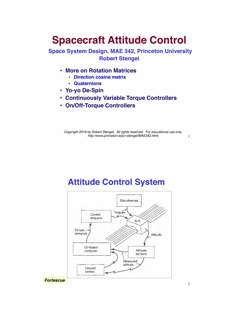
Attitude Control System

2Fortescue

3

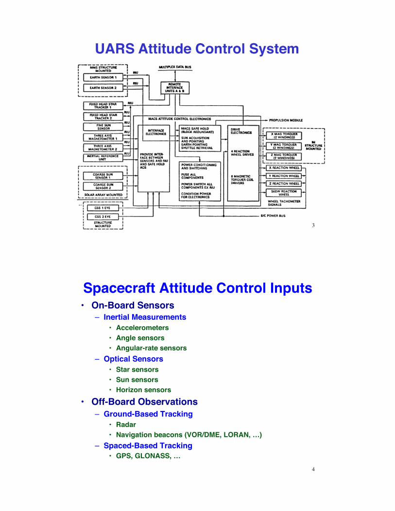
UARS Attitude Control System

Spacecraft Attitude Control Inputs•! On-Board Sensors

–! Inertial Measurements•! Accelerometers•! Angle sensors•! Angular-rate sensors

–! Optical Sensors•! Star sensors•! Sun sensors•! Horizon sensors

•! Off-Board Observations–! Ground-Based Tracking

•! Radar•! Navigation beacons (VOR/DME, LORAN, …)

–! Spaced-Based Tracking•! GPS, GLONASS, …

4

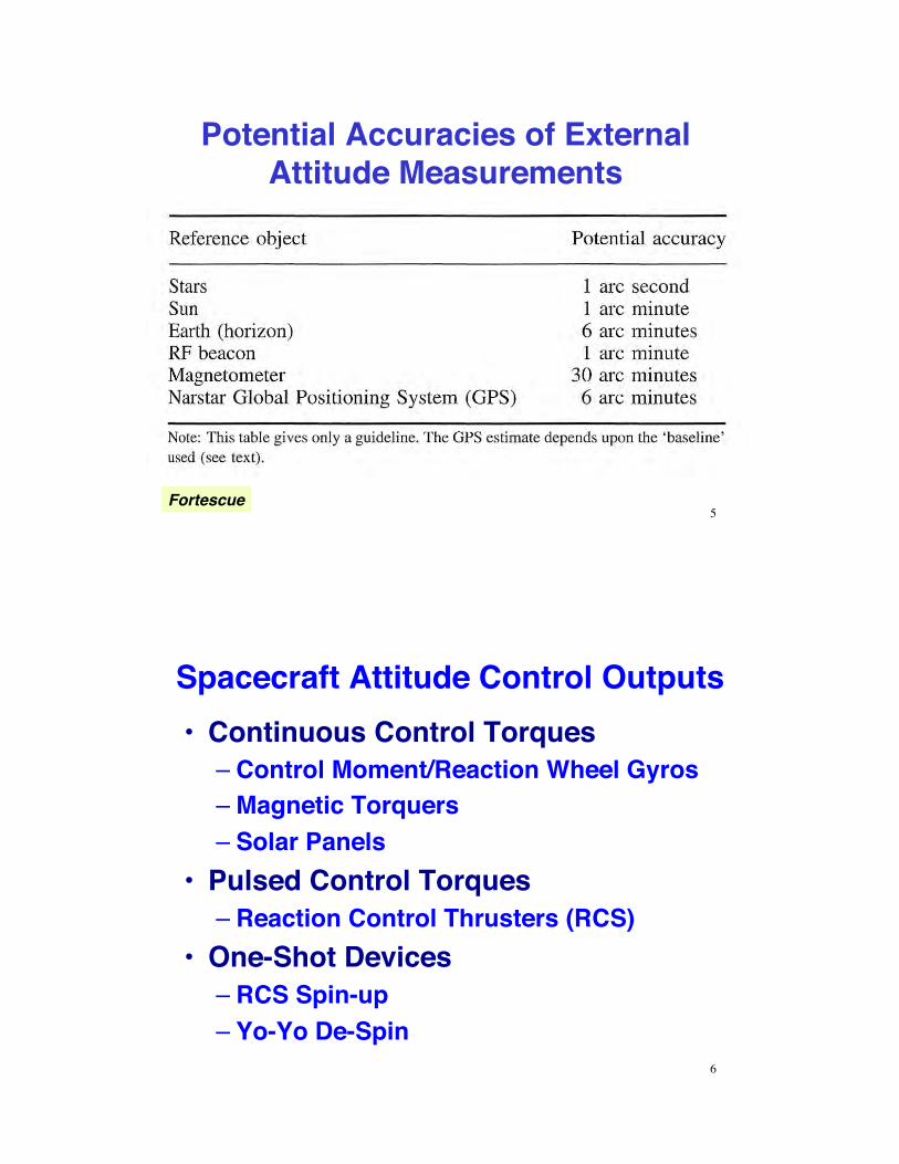
Potential Accuracies of External Attitude Measurements

Fortescue5

Spacecraft Attitude Control Outputs•! Continuous Control Torques

–!Control Moment/Reaction Wheel Gyros–!Magnetic Torquers–!Solar Panels

•! Pulsed Control Torques–!Reaction Control Thrusters (RCS)

•! One-Shot Devices–!RCS Spin-up–!Yo-Yo De-Spin

6

Spacecraft Attitude Disturbances•! External Torques

–! Solar radiation pressure–! Gravity gradient–! Magnetic fields–! Aerodynamics–! Can be put to good use if related to

attitude control objectives•! Vehicle-Based Torques

–! Mass movement–! Elasticity–! Out-gassing

7

More on Rotation Matrices and Quaternions!

8

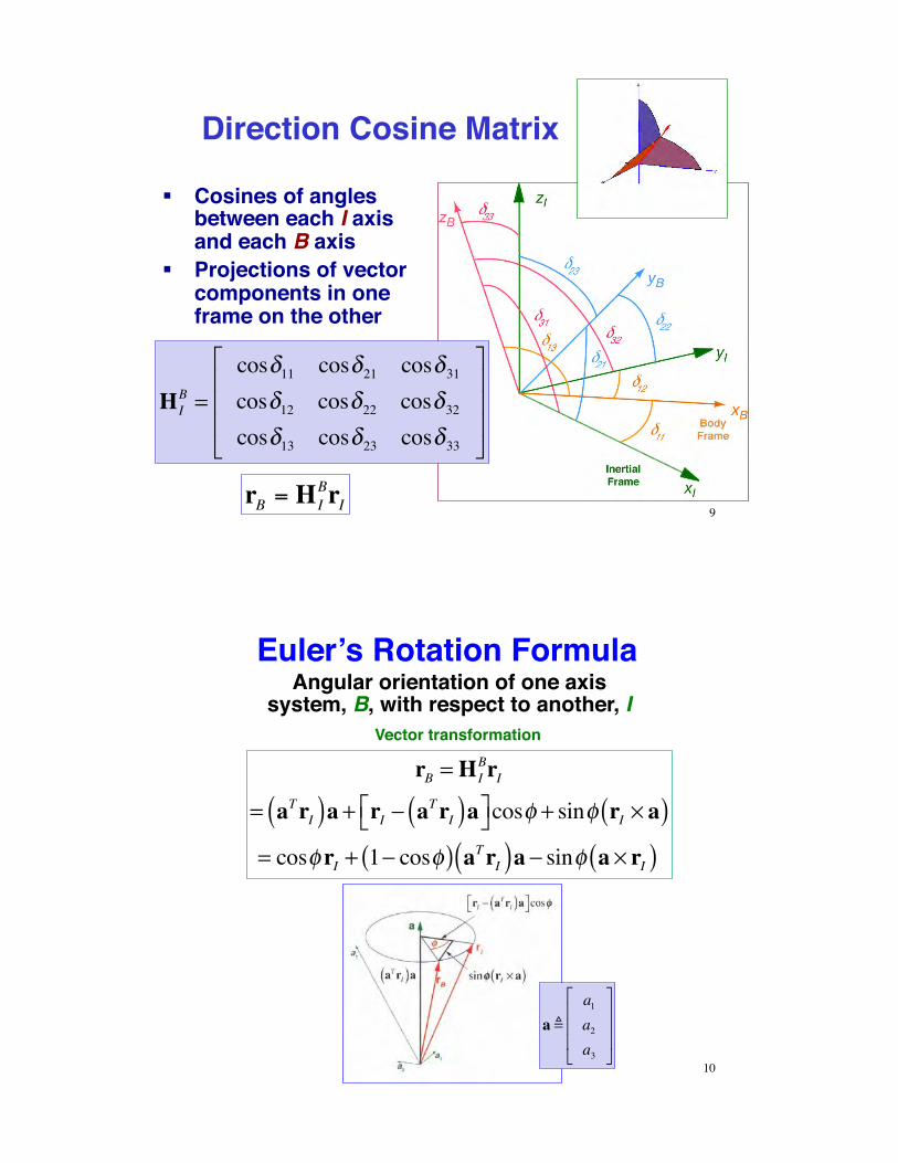
!! Cosines of angles between each I axis and each B axis

!! Projections of vector components in one frame on the other

H IB =

cos!11 cos!21 cos!31cos!12 cos!22 cos!32cos!13 cos!23 cos!33

"

#

$$$

%

&

'''

9

Direction Cosine Matrix

rB = H IBrI

Angular orientation of one axis system, B, with respect to another, I

10

Euler’s Rotation Formula

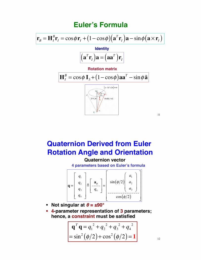
rB = H IBrI

= aTrI( )a + rI ! aTrI( )a"# $%cos& + sin& rI ' a( )

= cos& rI + 1! cos&( ) aTrI( )a ! sin& a ' rI( )

Vector transformation

a !a1a2a3

!

"

###

$

%

&&&

11

Euler’s FormularB = H I

BrI = cos! rI + 1" cos!( ) aTrI( )a " sin! a # rI( )

aTrI( )a = aaT( )rI

H IB = cos! I3 + 1" cos!( )aaT " sin! !a

Identity

Rotation matrix

Quaternion Derived from Euler Rotation Angle and Orientation

q =

q1q2q3q4

!

"

#####

$

%

&&&&&

!a'q4

!

"##

$

%&&=

sin ' 2( )a1a2a3

(

)

***

+

,

---

cos ' 2( )

!

"

######

$

%

&&&&&&

!! Not singular at ! = ±90°!! 4-parameter representation of 3 parameters;

hence, a constraint must be satisfied

12

qT q = q12 + q2

2 + q32 + q4

2

= sin2 ! 2( ) + cos2 ! 2( ) = 1

Quaternion vector4 parameters based on Euler’s formula

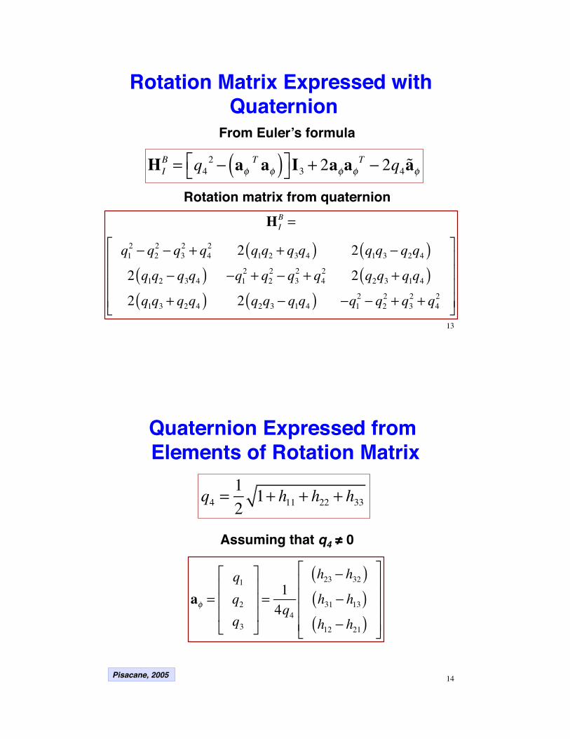
Rotation Matrix Expressed with Quaternion

13

H I

B = q42 ! a"

T a"( )#$ %&I3 + 2a"a"T ! 2q4 !a"

H IB =

q12 ! q2

2 ! q32 + q4

2 2 q1q2 + q3q4( ) 2 q1q3 ! q2q4( )2 q1q2 ! q3q4( ) !q1

2 + q22 ! q3

2 + q42 2 q2q3 + q1q4( )

2 q1q3 + q2q4( ) 2 q2q3 ! q1q4( ) !q12 ! q2

2 + q32 + q4

2

"

#

$$$$

%

&

''''

From Euler’s formula

Rotation matrix from quaternion

Quaternion Expressed from Elements of Rotation Matrix

14

q4 =121+ h11 + h22 + h33

a! =q1q2q3

"

#

$$$

%

&

'''= 14q4

h23 ( h32( )h31 ( h13( )h12 ( h21( )

"

#

$$$$

%

&

''''

Assuming that q4 " 0

Pisacane, 2005

Successive Rotations Expressed by Products of Quaternions and

Rotation Matrices

15

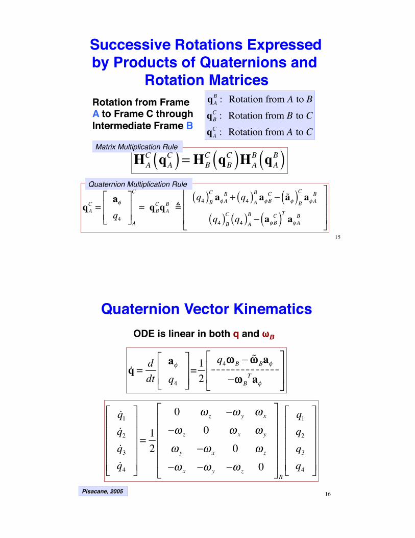
qAB : Rotation from A to BqBC : Rotation from B to CqAC : Rotation from A to C

Rotation from Frame A to Frame C through Intermediate Frame B

HAC qA

C( ) = HBC qB

C( )HAB qA

B( )

qAC =

a!q4

"

#$$

%

&''A

C

= qBCqA

B !q4( )B

C a!AB + q4( )A

B a!BC ( "a!( )B

Ca!A

B

q4( )BC q4( )A

B ( a!BC( )T a!AB

"

#

$$$

%

&

'''

Quaternion Multiplication Rule

Matrix Multiplication Rule

Quaternion Vector Kinematics

16

ODE is linear in both q and #B

!q = ddt

a!q4

"

#$$

%

&''= 12

q4(( B ) "(( Ba!)(( B

Ta!

"

#

$$

%

&

''

!q1!q2!q3!q4

!

"

#####

$

%

&&&&&

= 12

0 ' z (' y ' x

(' z 0 ' x ' y

' y (' x 0 ' z

(' x (' y (' z 0

!

"

#####

$

%

&&&&&B

q1q2q3q4

!

"

#####

$

%

&&&&&

Pisacane, 2005

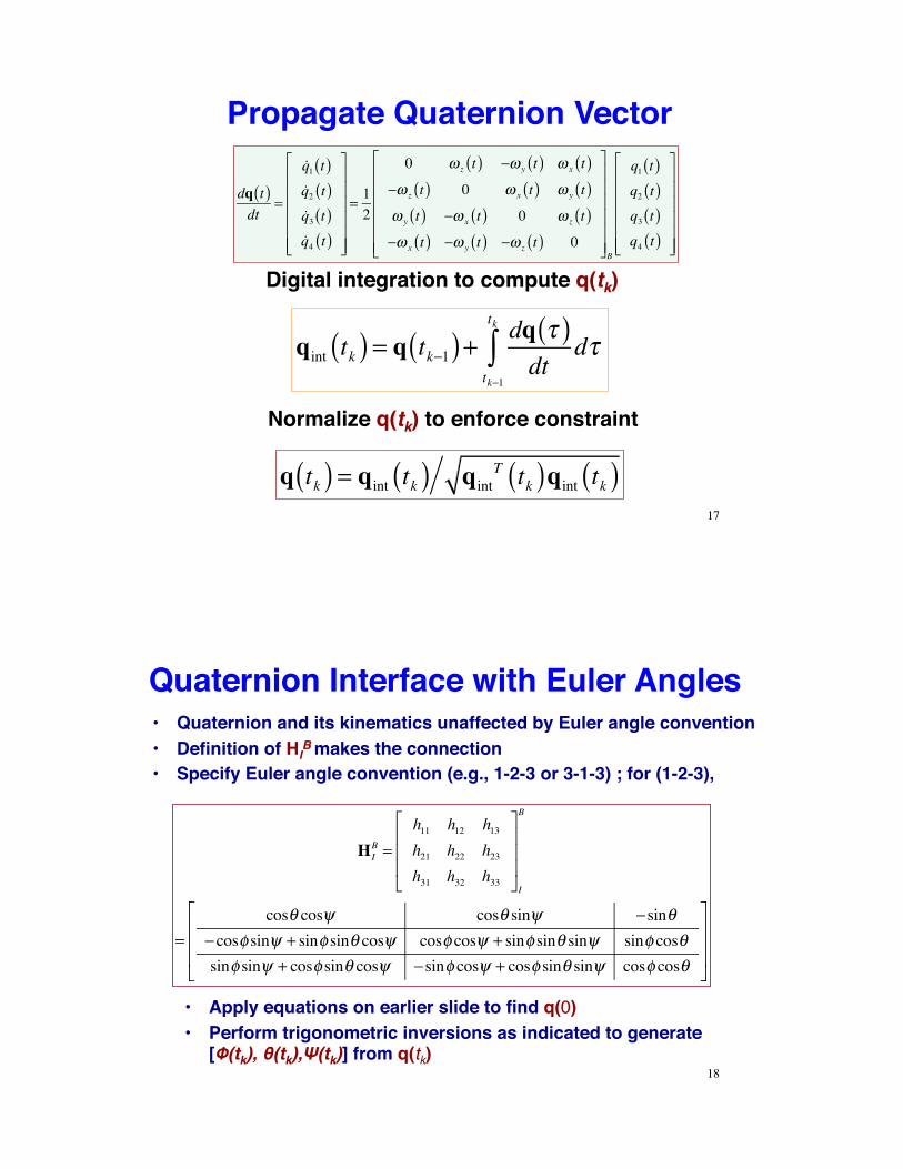
Propagate Quaternion Vector

17

dq t( )dt

=

!q1 t( )!q2 t( )!q3 t( )!q4 t( )

!

"

######

$

%

&&&&&&

= 12

0 ' z t( ) (' y t( ) ' x t( )(' z t( ) 0 ' x t( ) ' y t( )' y t( ) (' x t( ) 0 ' z t( )(' x t( ) (' y t( ) (' z t( ) 0

!

"

######

$

%

&&&&&&B

q1 t( )q2 t( )q3 t( )q4 t( )

!

"

######

$

%

&&&&&&

qint tk( ) = q tk!1( ) + dq "( )dt

d"tk!1

tk

#

Digital integration to compute q(tk)

Normalize q(tk) to enforce constraint

q tk( ) = qint tk( ) qintT tk( )qint tk( )

Quaternion Interface with Euler Angles

18

•! Quaternion and its kinematics unaffected by Euler angle convention•! Definition of HI

B makes the connection•! Specify Euler angle convention (e.g., 1-2-3 or 3-1-3) ; for (1-2-3),

H IB =

h11 h12 h13h21 h22 h23h31 h32 h33

!

"

###

$

%

&&&I

B

=cos' cos( cos' sin( )sin'

)cos* sin( + sin* sin' cos( cos* cos( + sin* sin' sin( sin* cos'sin* sin( + cos* sin' cos( )sin* cos( + cos* sin' sin( cos* cos'

!

"

###

$

%

&&&

•! Apply equations on earlier slide to find q(0)•! Perform trigonometric inversions as indicated to generate

["(tk), !(tk),#(tk)] from q(tk)

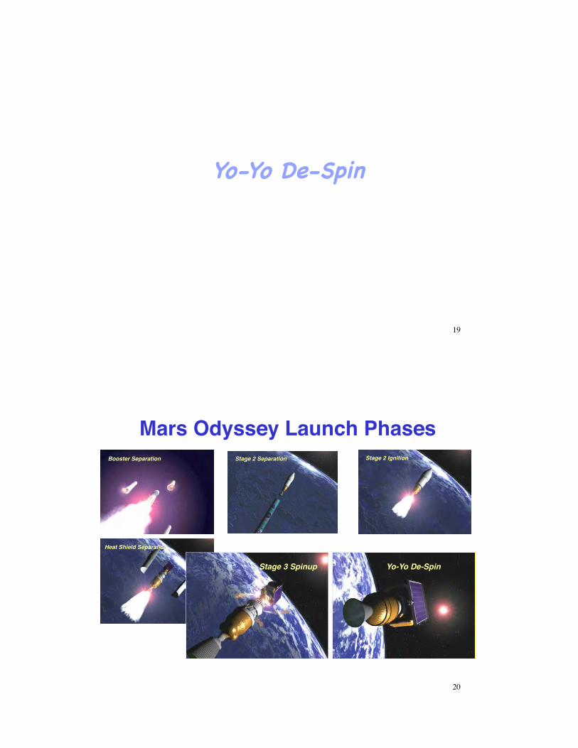
Yo-Yo De-Spin!

19

Mars Odyssey Launch PhasesBooster Separation Stage 2 Separation Stage 2 Ignition

Heat Shield Separation

Stage 3 Spinup Yo-Yo De-Spin

20

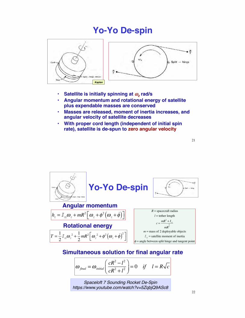
Yo-Yo De-spin

•! Satellite is initially spinning at !!z rad/s•! Angular momentum and rotational energy of satellite

plus expendable masses are conserved•! Masses are released, moment of inertia increases, and

angular velocity of satellite decreases•! With proper cord length (independent of initial spin

rate), satellite is de-spun to zero angular velocity

Kaplan

21

Yo-Yo De-spin

! final =! initialcR2 " l2

cR2 + l2#$%

&'(= 0 if l = R c

R = spacecraft radiusl = tether length

c = mR2 + Izz

mR22

m = mass of 2 deployable objectsI zz = satellite moment of inertia

! = angle between split hinge and tangent point

Angular momentum

Rotational energy

Simultaneous solution for final angular rate

hz = I zz! z +mR2 ! z +"

2 ! z + !"( )#$ %&

T = 1

2I zz! z

2 + 12mR2 ! z

2 +" 2 ! z + !"( )2#$

%&

22

Spaceloft 7 Sounding Rocket De-Spinhttps://www.youtube.com/watch?v=5ZqbjQ9ASc8

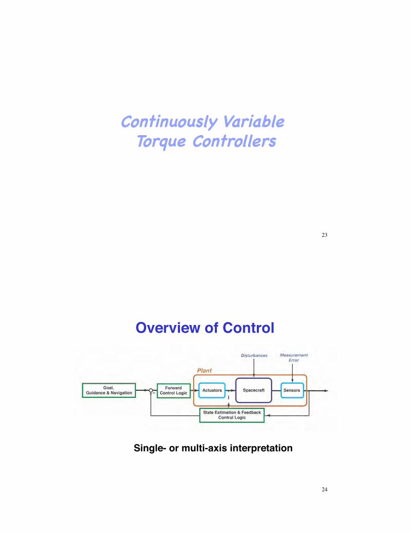
Continuously Variable Torque Controllers!

23

Overview of Control

24

Single- or multi-axis interpretation

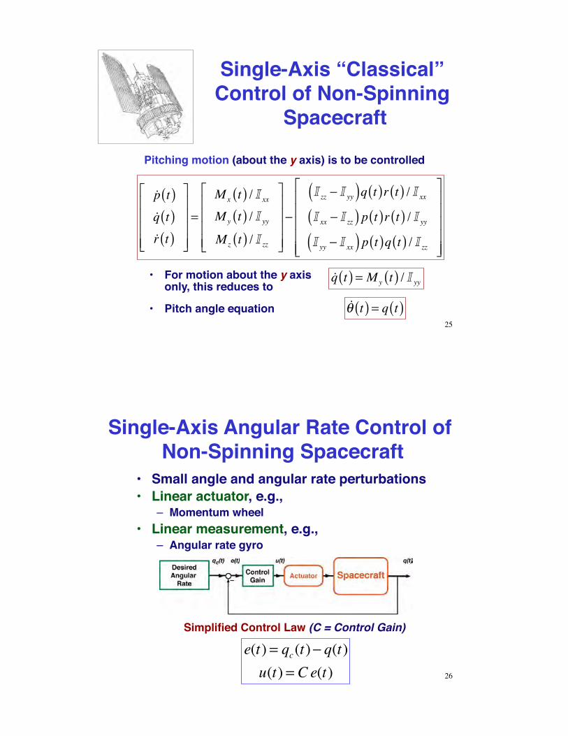
Single-Axis “Classical” Control of Non-Spinning

Spacecraft

Pitching motion (about the y axis) is to be controlled

!p t( )!q t( )!r t( )

!

"

####

$

%

&&&&

=

Mx t( ) / I xx

My t( ) / I yy

Mz t( ) / I zz

!

"

####

$

%

&&&&

'

I zz ' I yy( )q t( )r t( ) / I xx

I xx ' I zz( ) p t( )r t( ) / I yy

I yy ' I xx( ) p t( )q t( ) / I zz

!

"

#####

$

%

&&&&&

!q t( ) = My t( ) / I yy•! For motion about the y axis

only, this reduces to

!! t( ) = q t( )•! Pitch angle equation

25

Single-Axis Angular Rate Control of Non-Spinning Spacecraft

e(t) = qc(t)! q(t)u(t) = Ce(t)

Simplified Control Law (C = Control Gain)

•! Small angle and angular rate perturbations•! Linear actuator, e.g.,

–! Momentum wheel•! Linear measurement, e.g.,

–! Angular rate gyro

26

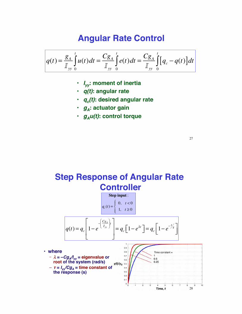
Angular Rate Control

•! Iyy: moment of inertia •! q(t): angular rate•! qc(t): desired angular rate•! gA: actuator gain •! gAu(t): control torque

q(t) = gA

I yy

u(t)0

t

! dt = CgAI yy

e(t)0

t

! dt = CgAI yy

qc " q(t)[ ]0

t

! dt

27

Step Response of Angular Rate Controller

q(t) = qc 1! e! CgA

Iyy

"

#$

%

&' t(

)

**

+

,

--= qc 1! e

.t() +, = qc 1! e! t /(

)*+,-

•! where! "" = –CgA/Iyy = eigenvalue or root of the system (rad/s)

–! $ = Iyy/CgA = time constant of the response (s)

Step input :

qc(t) =0, t < 01, t ! 0

"#$

%$

28

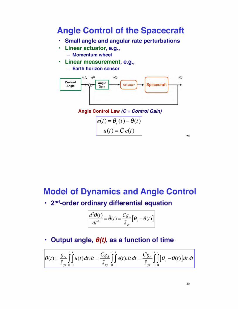
Angle Control of the Spacecraft

e(t) = !c(t)"!(t)u(t) = Ce(t)

Angle Control Law (C = Control Gain)

•! Small angle and angular rate perturbations•! Linear actuator, e.g.,

–! Momentum wheel•! Linear measurement, e.g.,

–! Earth horizon sensor

29

Model of Dynamics and Angle Control

!(t) = gA

I yy

u(t)0

t

" dt0

t

" dt = CgAI yy

e(t)0

t

" dt0

t

" dt = CgAI yy

!c #!(t)[ ]0

t

" dt dt0

t

"

•! 2nd-order ordinary differential equation

d 2!(t)dt 2

= !!!(t) = CgAI yy

!c "!(t)[ ]

•! Output angle, !(t), as a function of time

30

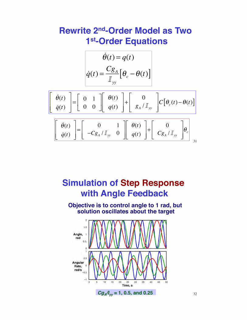
Rewrite 2nd-Order Model as Two 1st-Order Equations

!!(t) = q(t)

!q(t) = CgAI yy

!c "!(t)[ ]

!!(t)!q(t)

"

#$$

%

&''= 0 1

0 0"

#$

%

&'

!(t)q(t)

"

#$$

%

&''+

0gA / I yy

"

#$$

%

&''C !c(t)(!(t)[ ]

!!(t)!q(t)

"

#$$

%

&''=

0 1(CgA / I yy 0

"

#$$

%

&''

!(t)q(t)

"

#$$

%

&''+

0CgA / I yy

"

#$$

%

&''!c

31

Simulation of Step Response with Angle Feedback

Objective is to control angle to 1 rad, but solution oscillates about the target

CgA/Iyy = 1, 0.5, and 0.25 32

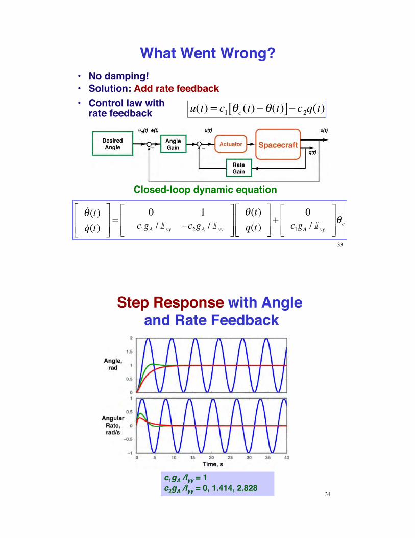
What Went Wrong?•! No damping!•! Solution: Add rate feedback

Closed-loop dynamic equation

u(t) = c1 !c (t) "!(t)[ ]" c2q(t)

!!(t)!q(t)

"

#$$

%

&''=

0 1(c1gA / I yy (c2gA / I yy

"

#$$

%

&''

!(t)q(t)

"

#$$

%

&''+

0c1gA / I yy

"

#$$

%

&''!c

•! Control law with rate feedback

33

c1gA /Iyy = 1 c2gA /Iyy = 0, 1.414, 2.828

Step Response with Angle and Rate Feedback

34

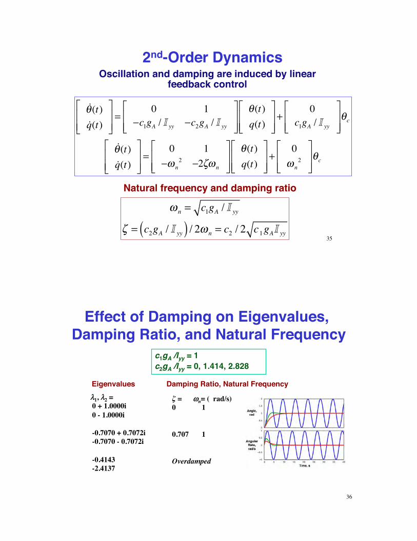
2nd-Order Dynamics

!!(t)!q(t)

"

#$$

%

&''=

0 1(c1gA / I yy (c2gA / I yy

"

#$$

%

&''

!(t)q(t)

"

#$$

%

&''+

0c1gA / I yy

"

#$$

%

&''!c

!!(t)!q(t)

"

#$$

%

&''=

0 1() n

2 (2*) n

"

#$$

%

&''

!(t)q(t)

"

#$$

%

&''+

0) n

2

"

#$$

%

&''!c

Oscillation and damping are induced by linear feedback control

! n = c1gA / I yy

" = c2gA / I yy( ) / 2! n = c2 / 2 c1gAI yy

Natural frequency and damping ratio

35

Effect of Damping on Eigenvalues, Damping Ratio, and Natural Frequency

""1, ""2 = 0 + 1.0000i 0 - 1.0000i

-0.7070 + 0.7072i -0.7070 - 0.7072i

-0.4143 -2.4137

Eigenvalues

! = !!n = ( rad/s) 0 1

0.707 1

Overdamped

Damping Ratio, Natural Frequency

c1gA /Iyy = 1 c2gA /Iyy = 0, 1.414, 2.828

36

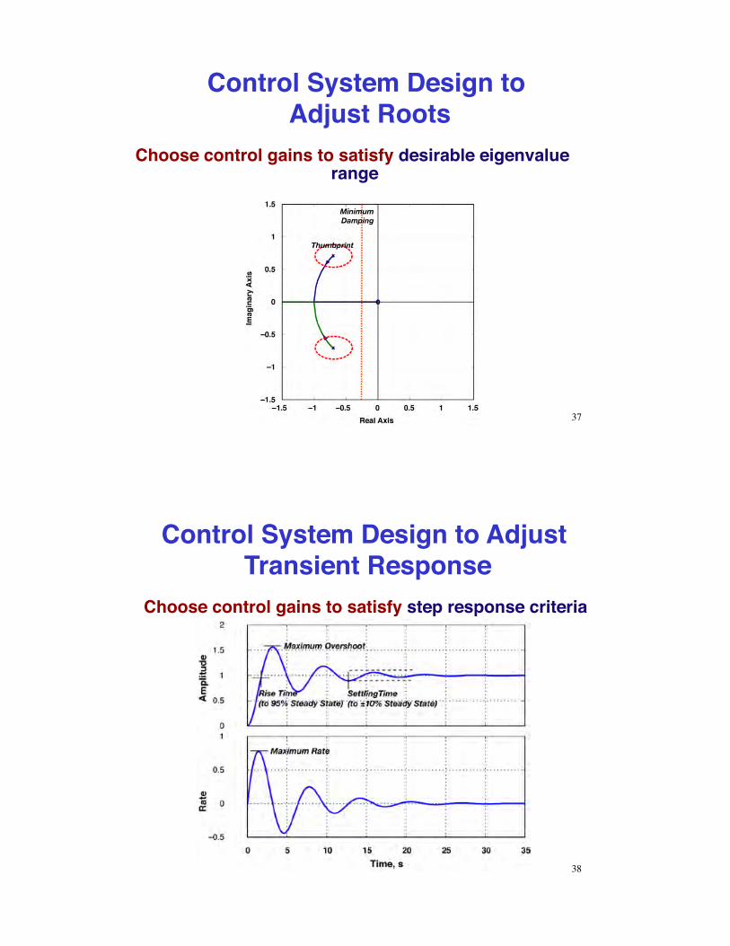
Control System Design to Adjust Roots

Choose control gains to satisfy desirable eigenvalue range

37

Control System Design to Adjust Transient Response

Choose control gains to satisfy step response criteria

38

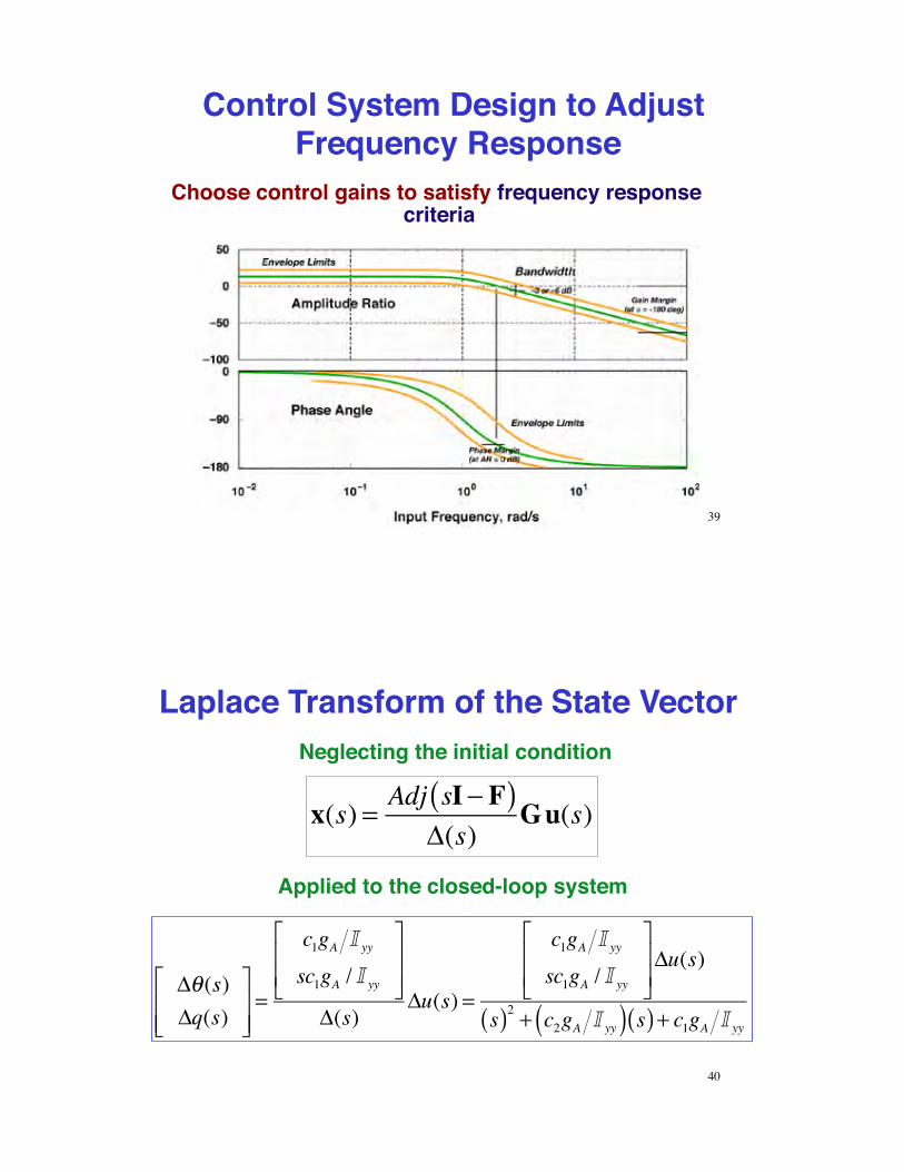
Control System Design to Adjust Frequency Response

Choose control gains to satisfy frequency response criteria

39

Laplace Transform of the State Vector

x(s) = Adj sI! F( )"(s)

Gu(s)

!"(s)!q(s)

#

$%%

&

'((=

c1gA I yy

sc1gA / I yy

#

$%%

&

'((

!(s)!u(s) =

c1gA I yy

sc1gA / I yy

#

$%%

&

'((!u(s)

s( )2 + c2gA I yy( ) s( ) + c1gA I yy

Applied to the closed-loop system

Neglecting the initial condition

40

Frequency Response of the System

!"( j#)!u( j#)

= #n2

j#( )2 + 2$#n j#( ) + #n2

!q( j")!u( j")

=j"( )"n

2

j"( )2 + 2#"n j"( ) + "n2

Angle Frequency Response

Rate Frequency Response

•!Bode plot–! 20 log(Amplitude Ratio) [dB] vs. log !!–! Phase angle (deg) vs. log !!

41

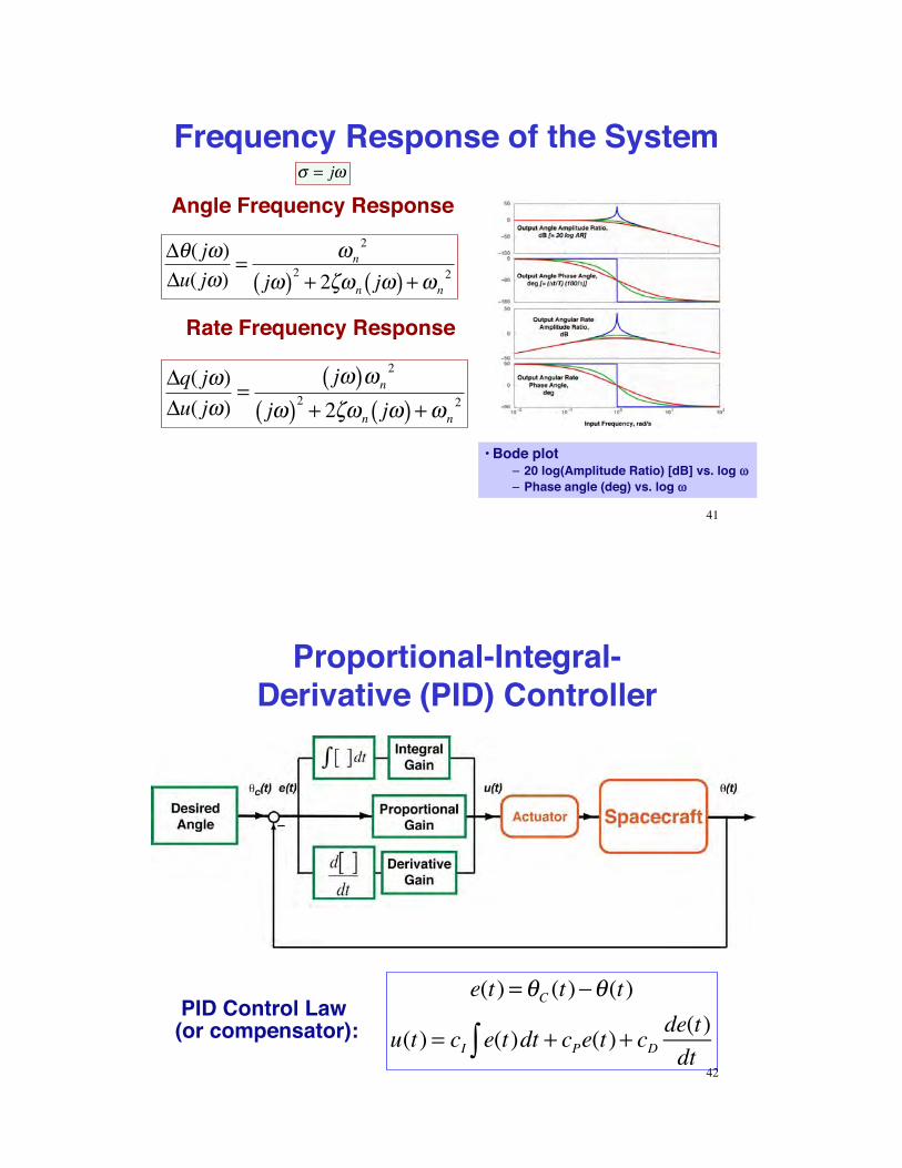
! = j"

Proportional-Integral-Derivative (PID) Controller

PID Control Law (or compensator):

e(t) = !C (t)"!(t)

u(t) = cI e(t)# dt + cPe(t)+ cDde(t)dt

42

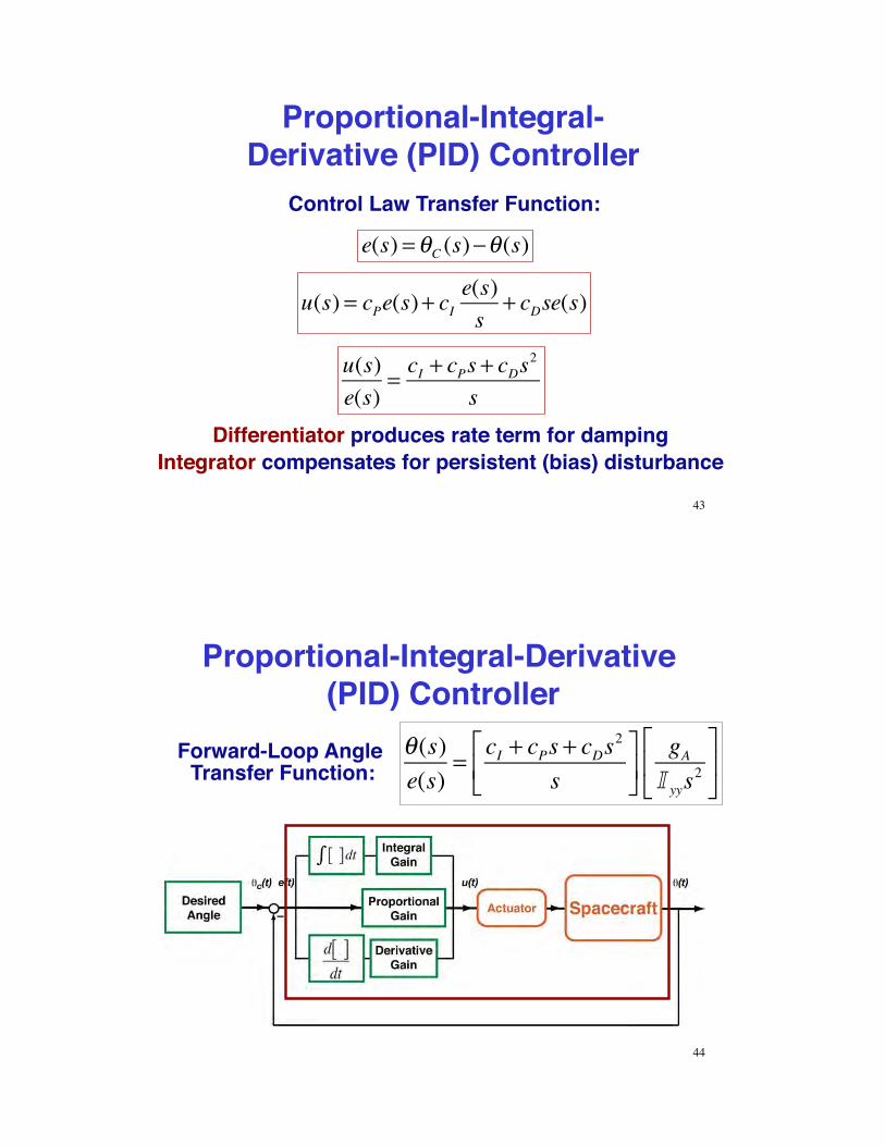
Proportional-Integral-Derivative (PID) Controller

Control Law Transfer Function:

e(s) = !C (s)"!(s)

Differentiator produces rate term for dampingIntegrator compensates for persistent (bias) disturbance

43

u(s) = cPe(s)+ cIe(s)s

+ cDse(s)

u(s)e(s)

= cI + cPs + cDs2

s

Proportional-Integral-Derivative (PID) Controller

Forward-Loop Angle Transfer Function:

!(s)e(s)

= cI + cPs + cDs2

s"

#$

%

&'

gAI yys

2

"

#$

%

&'

44

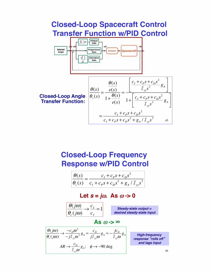
Closed-Loop Spacecraft Control Transfer Function w/PID Control

Closed-Loop Angle Transfer Function:

!(s)!c(s)

=

!(s)e(s)

1+ !(s)e(s)

=

cI + cPs + cDs2

I yys3 gA

"

#$

%

&'

1+ cI + cPs + cDs2

I yys3 gA

"

#$

%

&'

= cI + cPs + cDs2

cI + cPs + cDs2 + gA / I yys

345

Closed-Loop Frequency Response w/PID Control

Let s = j!!. As !! -> 0

!( j")!c ( j")

# cIcI

=1 Steady-state output = desired steady-state input

!(s)!c(s)

= cI + cPs + cDs2

cI + cPs + cDs2 + gA / I yys

3

As !! -> $

!( j" )!c( j" )

# $cD"2

$ jI yy"3 gA =

cDjI yy"

gA = $ jcDI yy"

gA

AR# cDI yy"

gA; % # $90 deg

High-frequency response rolls off

and lags input

46

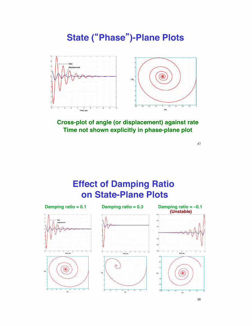
State ( Phase )-Plane Plots

Cross-plot of angle (or displacement) against rateTime not shown explicitly in phase-plane plot

47

Effect of Damping Ratio on State-Plane Plots

Damping ratio = 0.1 Damping ratio = 0.3 Damping ratio = –0.1 (Unstable)

48

On/Off-Torque Controllers!

49

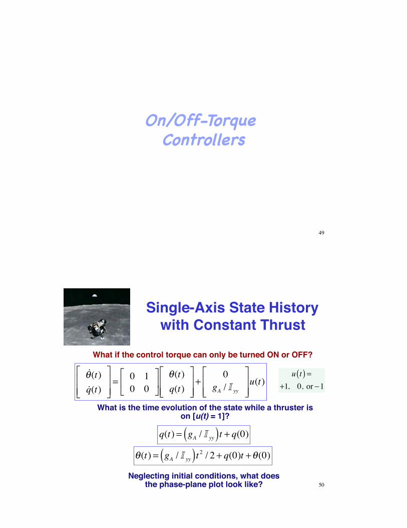
Single-Axis State History with Constant Thrust

!!(t)!q(t)

"

#$$

%

&''= 0 1

0 0"

#$

%

&'

!(t)q(t)

"

#$$

%

&''+

0gA / I yy

"

#$$

%

&''u(t)

What is the time evolution of the state while a thruster is on [u(t) = 1]?

q(t) = gA / I yy( )t + q(0)

!(t) = gA / I yy( )t 2 / 2 + q(0)t +!(0)Neglecting initial conditions, what does

the phase-plane plot look like?

What if the control torque can only be turned ON or OFF?

50

u t( ) =+1, 0, or !1

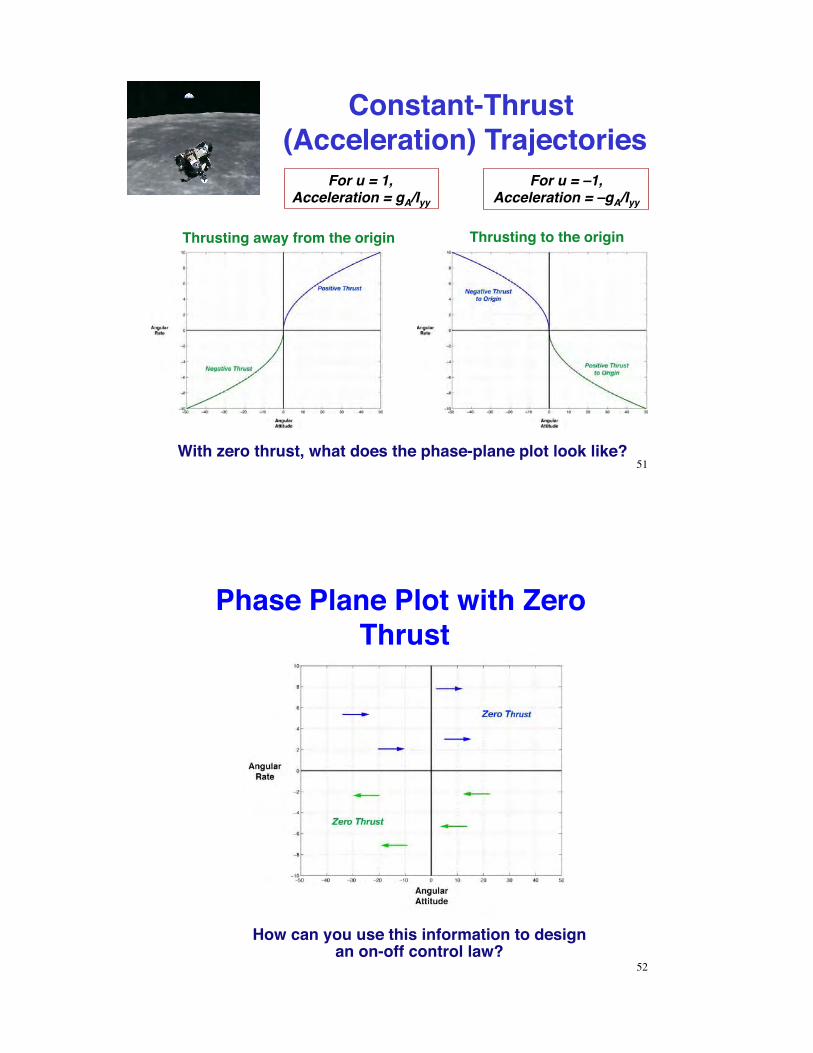
Constant-Thrust (Acceleration) Trajectories

For u = 1,Acceleration = gA/Iyy

Thrusting away from the origin Thrusting to the origin

With zero thrust, what does the phase-plane plot look like?

For u = –1,Acceleration = –gA/Iyy

51

Phase Plane Plot with Zero Thrust

52

How can you use this information to design an on-off control law?

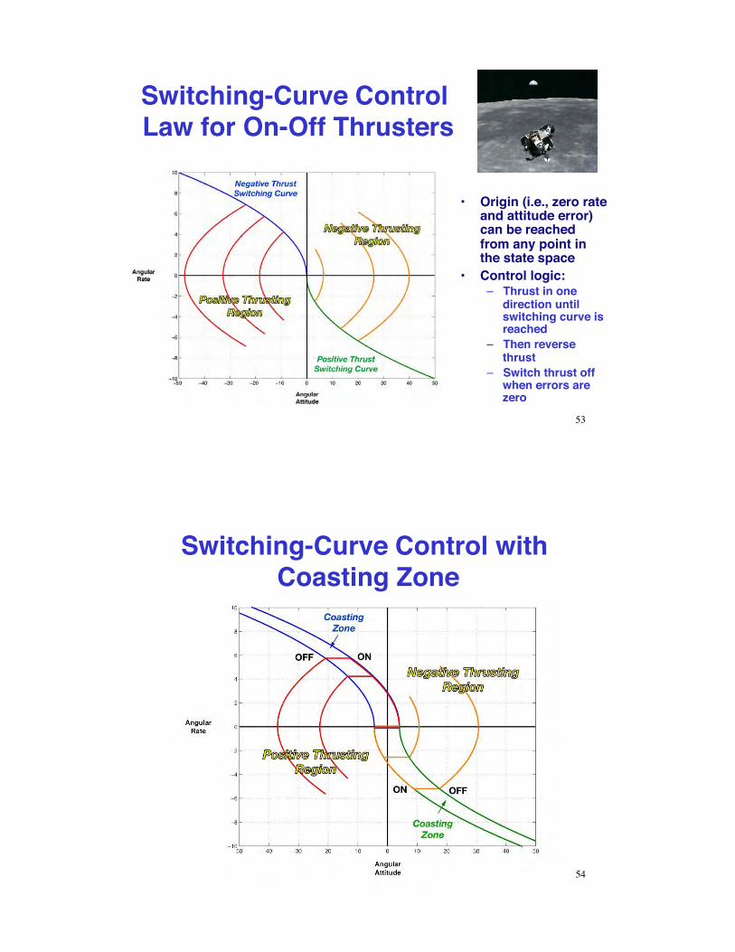
Switching-Curve Control Law for On-Off Thrusters

•! Origin (i.e., zero rate and attitude error) can be reached from any point in the state space

•! Control logic:–! Thrust in one

direction until switching curve is reached

–! Then reverse thrust

–! Switch thrust off when errors are zero

53

Switching-Curve Control with Coasting Zone

54

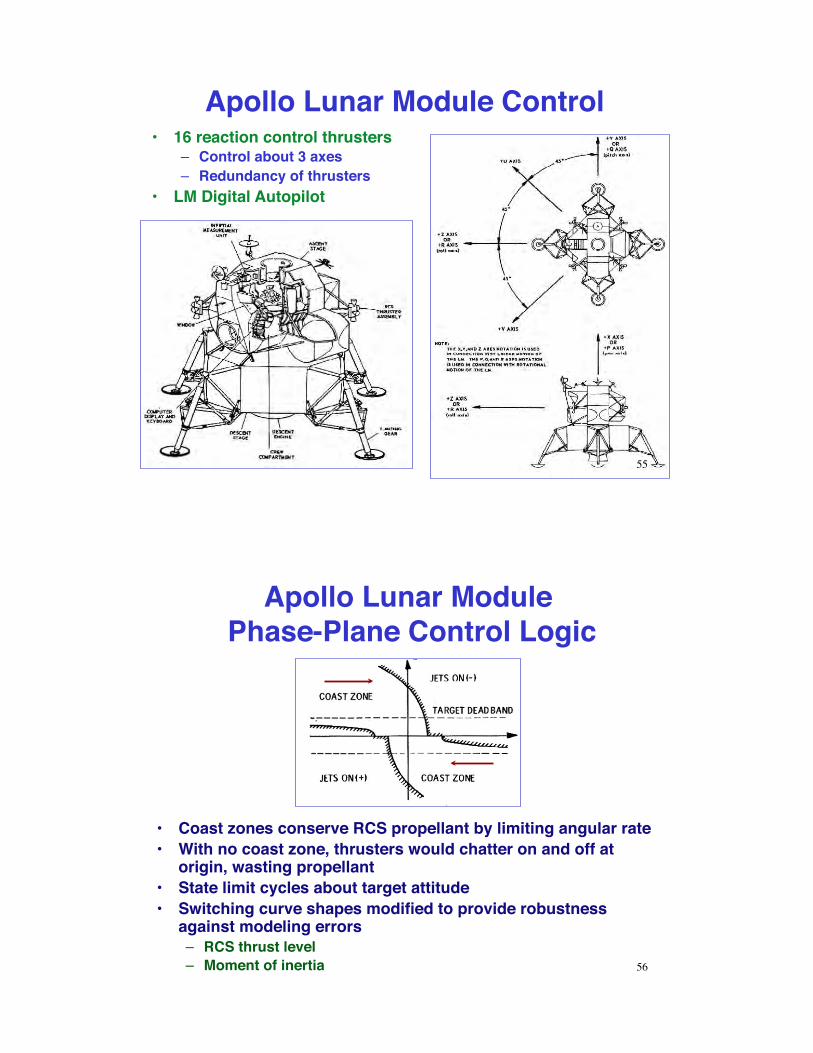
Apollo Lunar Module Control•! 16 reaction control thrusters

–! Control about 3 axes–! Redundancy of thrusters

•! LM Digital Autopilot

55

Apollo Lunar Module Phase-Plane Control Logic

•! Coast zones conserve RCS propellant by limiting angular rate•! With no coast zone, thrusters would chatter on and off at

origin, wasting propellant•! State limit cycles about target attitude•! Switching curve shapes modified to provide robustness

against modeling errors–! RCS thrust level–! Moment of inertia 56

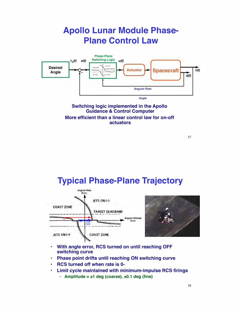
Apollo Lunar Module Phase-Plane Control Law

Switching logic implemented in the Apollo Guidance & Control Computer

More efficient than a linear control law for on-off actuators

57

Typical Phase-Plane Trajectory

•! With angle error, RCS turned on until reaching OFF switching curve

•! Phase point drifts until reaching ON switching curve•! RCS turned off when rate is 0-•! Limit cycle maintained with minimum-impulse RCS firings

–! Amplitude = ±1 deg (coarse), ±0.1 deg (fine)

58

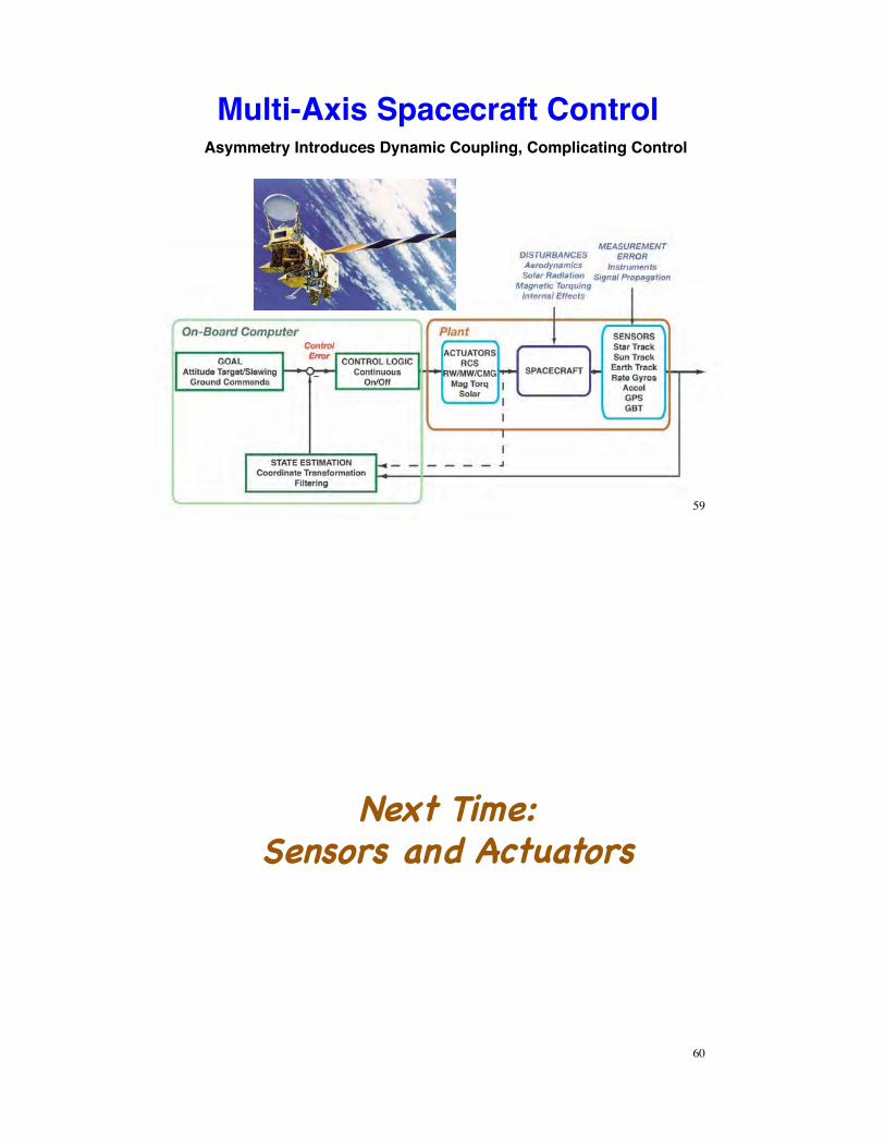
Multi-Axis Spacecraft Control

59

Asymmetry Introduces Dynamic Coupling, Complicating Control

Next Time:!Sensors and Actuators!

60

SSuupppplleemmeennttaall MMaatteerriiaall

61

62

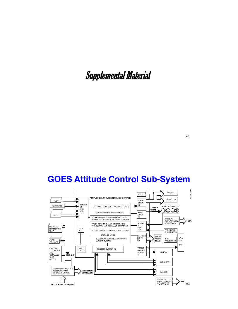
GOES Attitude Control Sub-System