aalborg universitet spacecraft attitude determination a
TRANSCRIPT
Aalborg Universitet
Spacecraft Attitude Determination
A Magnetometer Approach
Bak, Thomas
Publication date:1999
Document VersionOgså kaldet Forlagets PDF
Link to publication from Aalborg University
Citation for published version (APA):Bak, T. (1999). Spacecraft Attitude Determination: A Magnetometer Approach. Aalborg Universitetsforlag.
General rightsCopyright and moral rights for the publications made accessible in the public portal are retained by the authors and/or other copyright ownersand it is a condition of accessing publications that users recognise and abide by the legal requirements associated with these rights.
- Users may download and print one copy of any publication from the public portal for the purpose of private study or research. - You may not further distribute the material or use it for any profit-making activity or commercial gain - You may freely distribute the URL identifying the publication in the public portal -
Take down policyIf you believe that this document breaches copyright please contact us at [email protected] providing details, and we will remove access tothe work immediately and investigate your claim.
Downloaded from vbn.aau.dk on: February 02, 2022
Spacecraft Attitude Determination- a Magnetometer Approach
Ph.D. Thesis
Thomas Bak
Department of Control EngineeringAalborg University
Fredrik Bajers Vej 7, DK-9220 Aalborg Ø, Denmark.

ii
ISBN 87-90664-03-5Doc. no. D-99-4343August 1999Second edition, December 1999
Copyright 1999 c�
Thomas Bak
This thesis was typeset using Latex2e in report document class.
Drawings were made in CORELDRAWTM from Corel Corporation.Graphs were generated in MATLABTM from The MathWorks Inc.
Preface and Acknowledgments
This thesis is submitted in partial fulfillment of the requirements for the Doctorof Philosophy at the Department of Control Engineering, Aalborg University,Denmark. The work has been carried out in the period from December 1993 toAugust 1999 under the supervision of Professor Mogens Blanke.
I am thankful to my supervisor Professor Mogens Blanke for his guidanceduring the research program. His supervision and assistance in obtaining thefinancial support during the period of the work is also greatly appreciated.
I wish to thank Fred Hadaegh of the Jet Propulsion Laboratory, Control Anal-ysis Group, for giving me the opportunity to visit JPL during an eight monthperiod in 1996-1997 and work with an extraordinary group of people.
The access to magnetometer data from the Freja satellite was a courtesy ofGeoForschungsZentrum (GFZ), Potsdam, and the Aflvén Laboratory, KungligaTekniska Högskolan, Sweden.
Furthermore, I am most thankful to the staff at the Department of ControlEngineering for assistance and support. A special thanks to my office-mateand colleague Rafał Wisniewski, for his continued support during my writingof the thesis. I also greatly acknowledge the assistance from my other col-leagues within the Ørsted group: Søren Abildsten Bøgh, and Roozbeh Izadi-Zamanabadi. Thank you also to Martin Bak, who read through the manuscriptbefore I submitted it.
I also acknowledge the Ørsted Satellite Project and the Danish ResearchCouncil (STVF) under contract number 456/9601158 for financial support dur-ing my work.
August 1999, Aalborg, DenmarkThomas Bak
iii

Summary
This thesis describes the development of an attitude determination system forspacecraft based only on magnetic field measurements. The need for such sys-tem is motivated by the increased demands for inexpensive, lightweight solutionsfor small spacecraft. These spacecraft demands full attitude determination basedon simple, reliable sensors. Meeting these objectives with a single vector mag-netometer is difficult and requires temporal fusion of data in order to avoid localobservability problems. In order to guaranteed globally nonsingular solutions,quaternions are generally the preferred attitude specifier.
This thesis makes four main contributions. The first is the development of aquaternion based Kalman filter, which is linearized using an exponential map ofthe correction quaternion. The state space is reduced in dimension, and a covari-ance singularity is avoided. The second contributions is a detailed study of theinfluence of approximations in the modeling of the system. The quantitative ef-fects of errors in the process and noise statistics are discussed in detail. The thirdcontribution is the introduction of these methods to the attitude determinationon-board the Ørsted satellite. Implementation of the Ørsted filter is discussedand the predicted results are presented.
Finally the Kalman filter/smoother is applied to magnetometer data from theFreja satellite. Data is processed off-line, which enables us to estimate a highfidelity dynamic model of the spacecraft. Combined with a careful detection offield perturbations, the result is an significant improvement in accuracy whencompared to previous results. The results allow researchers to fully utilize theelectric field science measurements.
v

Synopsis
Denne Ph.D.-afhandling beskriver udviklingen af et retningsbestemmelsessys-tem til brug i forbindelse med satellitter. Systemet er baseret på anvendelsen afmagnetometre som eneste retningssensor. Brugen af sådanne systemer er mo-tiveret af de forøgede krav til billige, lette løsninger for små satellitter. Dissekræver fuld retningsinformation baseret på simple, pålidelige sensorer. For atkunne garantere globale ikke-singulære løsninger, kræves generelt quaternionstil beskrivelsen af retningen. At møde disse krav er vanskeligt med et enkelt vek-tor magnetometer instrument, og kræver tids fusion af data for at undgå proble-mer med lokal observerbarhed.
Denne afhandling har fire hovedbidrag. For det første udvikles et quaternionbasseret Kalman filter, som lineariseret ved hjælp af et exponentielt map af filterkorrektionen. Tilstandsrummet bliver reduceret i dimension and en kovariancesingularitet undgåes. Det andet bidrag er et detaljeret studie af inflydelsen fratilnærmelser i modelleringen af systemet. Den kvantitative effekt af fejl i processog støjbeskrivelserne diskuteres i detalje.
Det tredie bidrag er en introduktion of ovenstående metoder i forbindelse medretningsbestemmelse ombord på Ørsted satellitten. Implementation af Ørstedfiltret bliver diskuteret og de forudsagte resultater præsenteres. Endvidere eval-ueres resultater opnået med flight systemet fra Ørsted.
Endelige bliver et Kalman filter/smoother anvendt på magnetometer data fraFreja satellitten. Data processeres off-line, hvilket muliggør estimering af enmeget nøjagtig dynamisk model of rumfartøjet. Dette har i kombination medmed omhyggelig detektion af felt perturbationer, muliggjort en bestemmelse afretningen af Freja med hidtil uset nøjagtighed.
vii

Contents
List of Figures xiii
List of Tables xvii
Nomenclature xix
1 Introduction 11.1 Background and Motivation . . . . . . . . . . . . . . . . . . . . . . . 1
1.1.1 The Ørsted Case . . . . . . . . . . . . . . . . . . . . . . . . . 21.1.2 The Freja Case . . . . . . . . . . . . . . . . . . . . . . . . . . 31.1.3 Other Examples . . . . . . . . . . . . . . . . . . . . . . . . . . 4
1.2 Overview of Existing Methods . . . . . . . . . . . . . . . . . . . . . . 41.3 Objectives and Contributions . . . . . . . . . . . . . . . . . . . . . . . 51.4 Thesis Outline . . . . . . . . . . . . . . . . . . . . . . . . . . . . . . . 6
2 Attitude Determination in Perspective 92.1 Attitude Sensors . . . . . . . . . . . . . . . . . . . . . . . . . . . . . . 9
2.1.1 Inertial sensors . . . . . . . . . . . . . . . . . . . . . . . . . . 102.1.2 Reference Sensors . . . . . . . . . . . . . . . . . . . . . . . . 102.1.3 Sensor Summary . . . . . . . . . . . . . . . . . . . . . . . . . 15
2.2 Attitude Determination Methods . . . . . . . . . . . . . . . . . . . . . 162.2.1 Deterministic (point-by-point) solutions . . . . . . . . . . . . . 172.2.2 Recursive Estimation Algorithms . . . . . . . . . . . . . . . . 20
2.3 Summary . . . . . . . . . . . . . . . . . . . . . . . . . . . . . . . . . 21
3 Attitude and Spacecraft Motion Models 233.1 Rotations and Orthogonal Matrices . . . . . . . . . . . . . . . . . . . . 233.2 Attitude Representations . . . . . . . . . . . . . . . . . . . . . . . . . 273.3 Quaternions . . . . . . . . . . . . . . . . . . . . . . . . . . . . . . . . 293.4 Equations of Motion . . . . . . . . . . . . . . . . . . . . . . . . . . . 32
3.4.1 Attitude Kinematics . . . . . . . . . . . . . . . . . . . . . . . 32
ix
x Contents
3.4.2 Dynamics . . . . . . . . . . . . . . . . . . . . . . . . . . . . . 343.4.3 External Torques . . . . . . . . . . . . . . . . . . . . . . . . . 35
3.5 Summary . . . . . . . . . . . . . . . . . . . . . . . . . . . . . . . . . 37
4 Attitude Estimation 394.1 The Kalman Filter . . . . . . . . . . . . . . . . . . . . . . . . . . . . . 40
4.1.1 Process and Observation Models . . . . . . . . . . . . . . . . . 414.2 Operation of the Filter . . . . . . . . . . . . . . . . . . . . . . . . . . 42
4.2.1 Linear Models . . . . . . . . . . . . . . . . . . . . . . . . . . 444.3 Estimators for Nonlinear Systems . . . . . . . . . . . . . . . . . . . . 44
4.3.1 The Extended Kalman Filter . . . . . . . . . . . . . . . . . . . 454.4 Temporal Fusion of Data . . . . . . . . . . . . . . . . . . . . . . . . . 48
4.4.1 Information Flow . . . . . . . . . . . . . . . . . . . . . . . . . 494.5 Model Selection . . . . . . . . . . . . . . . . . . . . . . . . . . . . . . 51
4.5.1 Modeling Errors . . . . . . . . . . . . . . . . . . . . . . . . . 514.6 The Quaternion in the Kalman Filter . . . . . . . . . . . . . . . . . . . 56
4.6.1 Covariance Singularity . . . . . . . . . . . . . . . . . . . . . . 564.6.2 Quaternion Unity . . . . . . . . . . . . . . . . . . . . . . . . . 59
4.7 Quaternion Vector Filter . . . . . . . . . . . . . . . . . . . . . . . . . 604.7.1 Filter State . . . . . . . . . . . . . . . . . . . . . . . . . . . . 604.7.2 Filter Propagation . . . . . . . . . . . . . . . . . . . . . . . . . 614.7.3 Filter Update . . . . . . . . . . . . . . . . . . . . . . . . . . . 64
4.8 Summary . . . . . . . . . . . . . . . . . . . . . . . . . . . . . . . . . 65
5 Ørsted Attitude Estimation 695.1 Motivation and Related Work . . . . . . . . . . . . . . . . . . . . . . . 69
5.1.1 Introduction to the Ørsted Satellite . . . . . . . . . . . . . . . . 705.1.2 Measurement Package . . . . . . . . . . . . . . . . . . . . . . 725.1.3 The Attitude Control Subsystem . . . . . . . . . . . . . . . . . 74
5.2 The Attitude Estimation Problem . . . . . . . . . . . . . . . . . . . . . 765.2.1 System Design - Secondary Operation . . . . . . . . . . . . . . 78
5.3 Simulation Models . . . . . . . . . . . . . . . . . . . . . . . . . . . . 815.3.1 Spacecraft Truth Model . . . . . . . . . . . . . . . . . . . . . 825.3.2 Sensor Model . . . . . . . . . . . . . . . . . . . . . . . . . . . 83
5.4 Estimator Design . . . . . . . . . . . . . . . . . . . . . . . . . . . . . 875.4.1 Process Models . . . . . . . . . . . . . . . . . . . . . . . . . . 875.4.2 Process Noise Models . . . . . . . . . . . . . . . . . . . . . . 915.4.3 Sensor Model . . . . . . . . . . . . . . . . . . . . . . . . . . . 95
5.5 Performance Analysis for Secondary Operation . . . . . . . . . . . . . 965.5.1 Nominal Attitude . . . . . . . . . . . . . . . . . . . . . . . . . 975.5.2 Slow Drift . . . . . . . . . . . . . . . . . . . . . . . . . . . . . 1035.5.3 Large Initial Error . . . . . . . . . . . . . . . . . . . . . . . . 1045.5.4 Fault Scenario . . . . . . . . . . . . . . . . . . . . . . . . . . 107
Contents xi
5.6 Error Analysis . . . . . . . . . . . . . . . . . . . . . . . . . . . . . . . 1085.7 Summary . . . . . . . . . . . . . . . . . . . . . . . . . . . . . . . . . 111
6 Implementation and Results from Ørsted 1136.1 Implementation . . . . . . . . . . . . . . . . . . . . . . . . . . . . . . 113
6.1.1 Core Numerical Algorithms . . . . . . . . . . . . . . . . . . . 1146.1.2 Reference Field Implementation . . . . . . . . . . . . . . . . . 1196.1.3 ADS Implementation in Software . . . . . . . . . . . . . . . . 119
6.2 Results from Ørsted . . . . . . . . . . . . . . . . . . . . . . . . . . . . 1216.2.1 Attitude Time Histories . . . . . . . . . . . . . . . . . . . . . . 122
6.3 Summary . . . . . . . . . . . . . . . . . . . . . . . . . . . . . . . . . 126
7 Freja Attitude Estimation 1297.1 Motivation and Related Work . . . . . . . . . . . . . . . . . . . . . . . 129
7.1.1 Electric Field Experiment . . . . . . . . . . . . . . . . . . . . 1317.1.2 A Magnetometer based Approach for Freja . . . . . . . . . . . 132
7.2 The Attitude Problem . . . . . . . . . . . . . . . . . . . . . . . . . . . 1337.2.1 Magnetometer Calibration . . . . . . . . . . . . . . . . . . . . 1337.2.2 Reference Model Accuracy . . . . . . . . . . . . . . . . . . . . 1347.2.3 Accuracy of Dynamic Model . . . . . . . . . . . . . . . . . . . 135
7.3 Estimator Design . . . . . . . . . . . . . . . . . . . . . . . . . . . . . 1357.3.1 Smoothing . . . . . . . . . . . . . . . . . . . . . . . . . . . . 1367.3.2 Process Model . . . . . . . . . . . . . . . . . . . . . . . . . . 137
7.4 Performance Analysis . . . . . . . . . . . . . . . . . . . . . . . . . . . 1397.4.1 Attitude Reconstruction Results . . . . . . . . . . . . . . . . . 141
7.5 Perspective . . . . . . . . . . . . . . . . . . . . . . . . . . . . . . . . 1467.6 Summary . . . . . . . . . . . . . . . . . . . . . . . . . . . . . . . . . 147
8 Conclusion and Recommendations 1498.1 Conclusion . . . . . . . . . . . . . . . . . . . . . . . . . . . . . . . . 1498.2 Recommendations . . . . . . . . . . . . . . . . . . . . . . . . . . . . . 151
A Coordinate Systems 153
B Satellite and Space Environmental Models 157B.1 Atmospheric Density Model . . . . . . . . . . . . . . . . . . . . . . . 157B.2 Orbit Propagation Models . . . . . . . . . . . . . . . . . . . . . . . . . 157
B.2.1 Precision . . . . . . . . . . . . . . . . . . . . . . . . . . . . . 159B.3 Geomagnetic Reference Field Model . . . . . . . . . . . . . . . . . . . 160
Bibliography 161

List of Figures
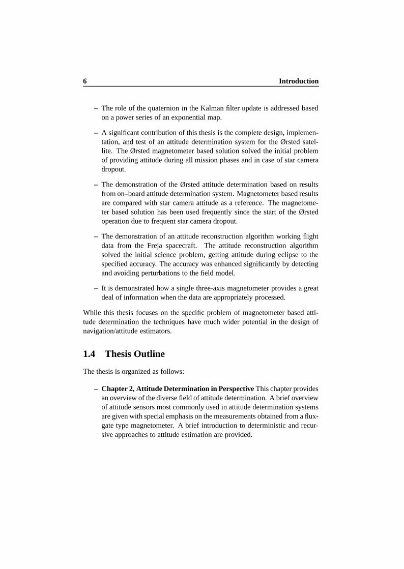
1.1 The magnetometer used on the Ørsted satellite (right photo). The mag-netometer is mounted on an instrument platform with a star camera(left photo) . . . . . . . . . . . . . . . . . . . . . . . . . . . . . . . . 3
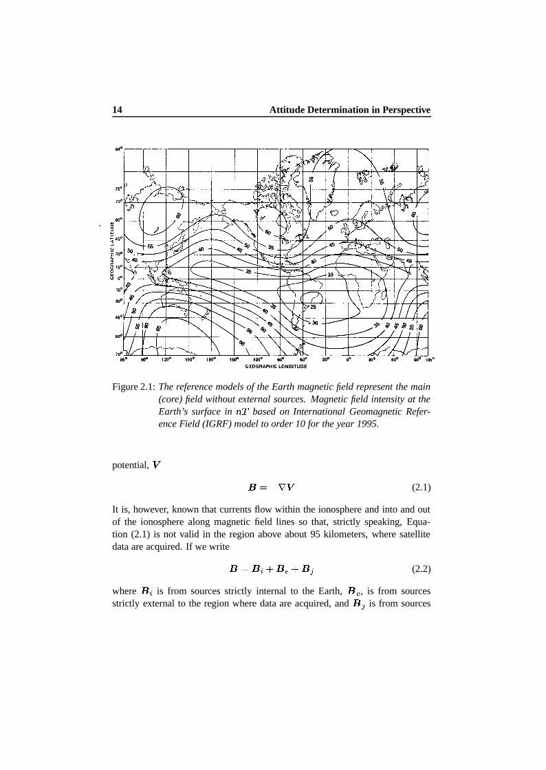
2.1 The reference models of the Earth magnetic field represent the main(core) field without external sources. Magnetic field intensity at theEarth’s surface in ��� based on International Geomagnetic ReferenceField (IGRF) model to order 10 for the year 1995 . . . . . . . . . . . 14
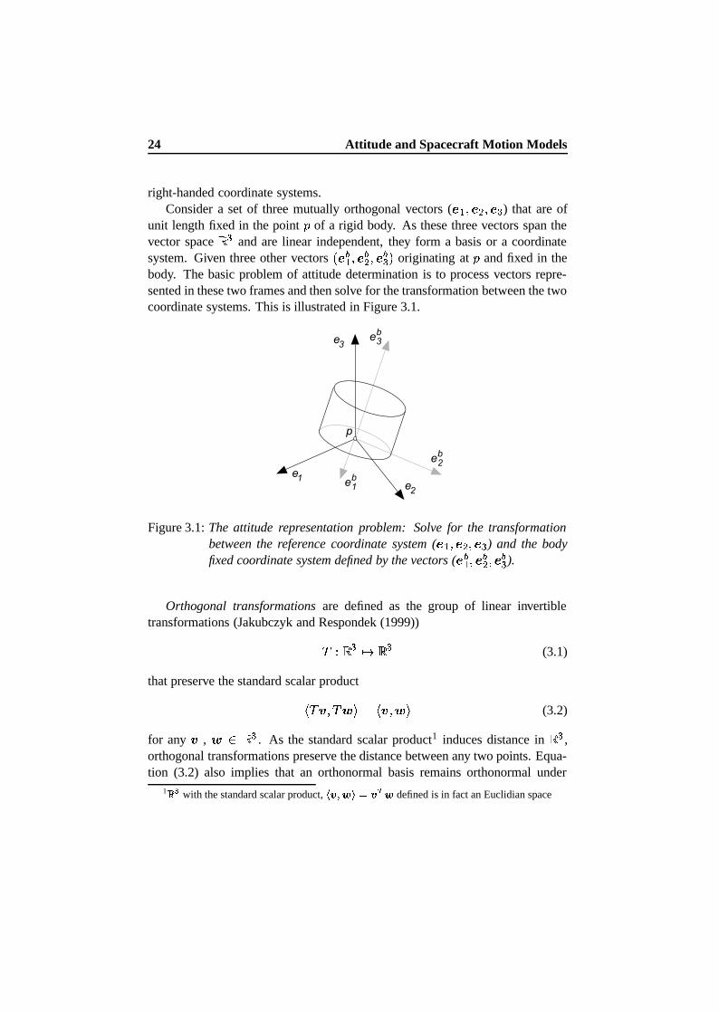
3.1 The attitude representation problem: Solve for the transformation be-tween the reference coordinate system ( ����������� ) and the body fixedcoordinate system defined by the vectors ( ���� ����� ����� ) . . . . . . . . . . 24
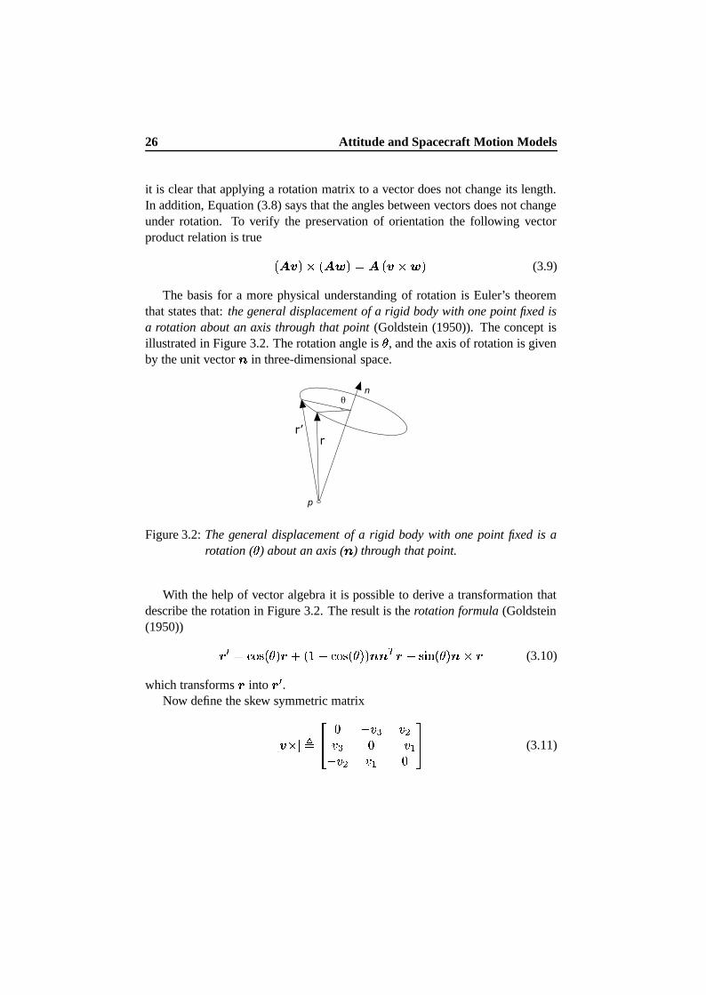
3.2 The general displacement of a rigid body with one point fixed is a ro-tation ( � ) about an axis ( � ) through that point . . . . . . . . . . . . . 26
3.3 Typical torques on a small spacecraft as a function of orbital altitudeabove Earth’s surface (Bryson (1994)) . . . . . . . . . . . . . . . . . 36
4.1 Kalman filter flow. Measurements, ������� are used to update the esti-mate �� ������� ����� . An a priori estimate, �� ��� ����� , for the next measurementinstance is found based on a process model . . . . . . . . . . . . . . 40
4.2 Kalman filter information flow schematic . . . . . . . . . . . . . . . . 50
5.1 The Ørsted satellite. The main body is 600 � 450 � 300 mm and thetotal weight is 62 kg. Instruments are placed on the 8 meter boom. Thevector magnetometer is placed in the gondola . . . . . . . . . . . . . 71
5.2 The attitude control system configuration. The main components aresensors, attitude determination, attitude control, and actuators . . . . . 76
5.3 Conceptual diagram of the Ørsted attitude estimation in secondary op-eration. Besides the core estimation algorithms in observational updateand propagation, additional support functions are required . . . . . . . 78
5.4 Ørsted alignment tree . . . . . . . . . . . . . . . . . . . . . . . . . . 815.5 Conceptual diagram of the Ørsted simulation model . . . . . . . . . . 82
xiii
xiv List of Figures
5.6 Magnitude discrepancies between IGRF field models. (a) Freja dataand results from an 8th order model. (standard deviation 86 nT). (b)Discrepancy between 8th and 10th order models (standard deviation28 nT) . . . . . . . . . . . . . . . . . . . . . . . . . . . . . . . . . . 84
5.7 Power spectral density plot for the magnitude error in Figure 5.6.a . . 855.8 Discrepancy IGRF 8th order model and simulation model. (a)-(c) x,
y, z components of error in ECEF coordinates (standard deviation:50 nT). (d) Angular error (standard deviation: 0.08 deg.) . . . . . . . . 86
5.9 Aerodynamic drag torque in the spacecraft body frame. The controlsystem keeps the satellite within "! deg. from local vertical with amaximum yaw deviation of 20 deg.. The # axis is approximately per-pendicular to the orbit plane . . . . . . . . . . . . . . . . . . . . . . . 90
5.10 Nominal performance – aligned with nadir by the control system.Pitch/roll/yaw relative to the local LVLH frame. Angular velocity rela-tive to inertial frame. The nominal angular velocity in # , and $ is zero,while the % component is approximately &'�(&*) �� rad/sec . . . . . . . 98
5.11 Nominal performance. Pitch/roll/yaw and angular velocity estimationerror for the P1 process model. Two standard deviation profiles arebased on diagonal elements from the estimated covariance matrix (dot-ted lines) . . . . . . . . . . . . . . . . . . . . . . . . . . . . . . . . . 99
5.12 Nominal performance. (a) yaw error for P1 model with standard de-viation envelope. (b) corresponding aerodynamic drag torque in bodyframe, $ direction. (c) angular distance between geomagnetic field vec-tor and the body $ axis . . . . . . . . . . . . . . . . . . . . . . . . . . 100
5.13 Nominal performance. Normalized state error . . . . . . . . . . . . . 1005.14 Nominal performance. Innovation sequence for the P1 process model.
Standard deviation profiles are based on diagonal elements from+ �-, ��� ����� +/.�103254�6 (dotted lines) . . . . . . . . . . . . . . . . . . . 1025.15 Nominal performance. Pitch/roll/yaw and angular velocity estimation
error for the P2 process model. Two standard deviation profiles arebased on diagonal elements from the estimated covariance matrix (dot-ted lines) . . . . . . . . . . . . . . . . . . . . . . . . . . . . . . . . . 103
5.16 Nominal performance. Aerodynamic drag torques in the LVLH frame.(a), (c) estimated and true �17 and ��8 drag torques. (b), (d) estimationerror. Standard deviation profiles are based on diagonal elements fromthe estimated covariance matrix (dotted lines) . . . . . . . . . . . . . 104
5.17 Slow spin – the satellite spins slowly about the $ -axis. Pitch/roll/yawrelative to local LVLH frame. Angular velocity relative to inertial frame 105
5.18 Pitch/roll/yaw and angular velocity estimation error for the P1 processmodel. Two standard deviation profiles are based on diagonal elementsfrom the estimated covariance matrix (dotted lines) . . . . . . . . . . 106
List of Figures xv
5.19 Large initial error – the satellite is offset 40, 30 and 60 deg. in the threeaxes. Pitch/roll/yaw relative to local LVLH frame. Angular velocityrelative to inertial frame . . . . . . . . . . . . . . . . . . . . . . . . . 107
5.20 Convergence of the P1 process model. The estimate converges froman initial knowledge error of 40, 30 and 60 deg. in the three axes. Theapproximate convergence time is 0.5 orbit . . . . . . . . . . . . . . . 108
5.21 Fault scenario - camera blackout after 200 minutes. In plot a) reconfig-uration is performed. In b) the attitude determination is not reconfigured 109
6.1 Schematically overview of the covariance prediction implemented onØrsted. Bierman’s square root free measurement update is combinedwith Thornton’s temporal update . . . . . . . . . . . . . . . . . . . . 118
6.2 On-board geomagnetic field model. Three components of the refer-ence field in orbital positions distributed over 24 hours. Discrepancybetween Ada fixed point implementation and Matlab 8th order model . 119
6.3 Context diagram for the ACS main tasks . . . . . . . . . . . . . . . . 1206.4 Ørsted results from orbits 2535-2538 (August 18 1999 UTC:
12:34:38). Pitch/roll/yaw estimates from the star camera (left) and theestimates based on data from the magnetometer (right). The attitude isgiven relative to LVLH . . . . . . . . . . . . . . . . . . . . . . . . . 123
6.5 Ørsted results from orbits 2535-2538 (August 18 1999 UTC:12:34:38). Pitch/roll/yaw discrepancies between star camera and mag-netometer based estimates of the attitude . . . . . . . . . . . . . . . . 124
6.6 Ørsted results from orbits 2539-2542 (August 18 1999 UTC:19:07:56). Pitch/roll/yaw estimates from the star camera (left) and theestimates based on data from the magnetometer (right). The attitude isgiven relative to LVLH . . . . . . . . . . . . . . . . . . . . . . . . . 125
6.7 Ørsted results from orbits 2539-2542 (August 18 1999 UTC:19:07:56). Pitch/roll/yaw discrepancies between star camera and mag-netometer based estimates of the attitude . . . . . . . . . . . . . . . . 126
7.1 The Freja satellite . . . . . . . . . . . . . . . . . . . . . . . . . . . . 1307.2 Attitude determination solution. Inertial magnetic field vectors from
the IGRF model are combined with measured vectors in a forward fil-tering pass. The state estimate is improved by backward smoothing ofthe covariance and state . . . . . . . . . . . . . . . . . . . . . . . . . 136
7.3 Freja passage over the auroral oval. Orbit 7281, data from Prince Al-bert and Esrange ground stations . . . . . . . . . . . . . . . . . . . . 140
7.4 Magnetic field measured by Freja F2 magnetometer, orbit 7281. Thefigures show the magnetic field projected onto the # , % and $ axis ofthe magnetometer and the field strength . . . . . . . . . . . . . . . . . 140
7.5 Orbit 7281 – Estimated and measured magnetic field measurements . . 1427.6 Measurement residual time histories . . . . . . . . . . . . . . . . . . 143
xvi List of Figures
7.7 Detection of magnetic disturbance by CUSUM log-likelihood test . . . 1457.8 Freja orbit 7281. Estimated spin axis azimuth and declination in ECI.
Estimated spin axis inertia . . . . . . . . . . . . . . . . . . . . . . . 1467.9 Freja orbit 7281. Squared covariance estimate on 9� . (a) covariance
after forward pass; (b) covariance after backward smoothing . . . . . . 147
A.1 Earth Centered Inertial (ECI) and Earth Centered Earth Fixed (ECEF)coordinate systems . . . . . . . . . . . . . . . . . . . . . . . . . . . . 153
A.2 Ørsted and Freja SCB coordinate systems . . . . . . . . . . . . . . . . 154A.3 Local Vertical Local Horizontal coordinate system . . . . . . . . . . . 155
B.1 Discrepancy between SPG4 prediction based on TLE and actual statevectors from SAMPEX . . . . . . . . . . . . . . . . . . . . . . . . . 159
List of Tables
2.1 Summary of typical attitude determination sensors. Performance,weight, power and characteristics are listed . . . . . . . . . . . . . . . 16
2.2 Summary of common point estimation attitude algorithms . . . . . . . 19
3.1 Parameterizations of the rotation group :<; 2>=�6 . Common parametersused in attitude control systems . . . . . . . . . . . . . . . . . . . . . . 28
4.1 Summary of Kalman filter. Linearizations and transition matrix are de-fined in the text above. . . . . . . . . . . . . . . . . . . . . . . . . . . 66
5.1 Operational parameters of the Ørsted satellite. Ørsted was launched onFebruary 23, 1999 . . . . . . . . . . . . . . . . . . . . . . . . . . . . . 72
5.2 Overview of the Ørsted Instruments package . . . . . . . . . . . . . . . 735.3 Parameters defining the spectral densities of the process and noise for
the two models P1 and P2 and the measurement noise covariance. . . . 965.4 Error analysis, systematic errors in the simulation model. . . . . . . . . 110
6.1 Implementation - code size Ørsted ADS modules. The total magnetome-ter related ADS code is responsible for 22% of the total ACS code. . . . 120
7.1 Operational parameters of the Freja satellite. Freja was launched onOctober 7, 1992 . . . . . . . . . . . . . . . . . . . . . . . . . . . . . . 131
7.2 Parameters defining the spectral densities of the process noise as well asthe measurement noise covariance for Freja . . . . . . . . . . . . . . . 139
7.3 Freja attitude information . . . . . . . . . . . . . . . . . . . . . . . . . 145
xvii

Nomenclature
Symbols
?General = � = rotation matrix@ 2BA 6 Wahba’s loss functionC Three dimensional real space:D; 2>=E6 Special orthogonal group of order threeFRotation vectorGThe quaternion groupCReal space: Unit sphere in four-dimensional space: Unit sphere in three-dimensional spaceHJILeft operator, matrix representation of quaternion productK IRight operator, matrix representation of quaternion productL 2NMB6 Skew symmetric matrix ( OP�QO 6 , quaternion kinematics.R 2NMB6 Angular velocity vector.S � 2>MB6 Angular momentum� 2>MB6 Torque vectorTMoments of inertia tensor 2>= � =E6R � 2NMB6 Angular velocity in the body frame�VUWU 2NMB6 Gravity gradient torque vectorX � 2NMB6 Unit zenith vector, gravity gradient modeling� State vectorY 2ZA[6 Continuous time process model\ 2NMB6 Deterministic control input] 2NMB6 Brownian motion^ 2NMB6 Continuous noise input to process model_ 2NMB6 Spectral density of of ^ 2NMB6� � Discrete observation vectorS 2ZA[6 Observation model` � Discrete noise on observation model
xix
xx Nomenclature
03254�6 Discrete observation noise covariance��ba � c Estimated conditional mean of state, a � c Conditional covarianced c Sequence of observationse� ��� ����� Error in the prediction at time M � given observations up to time M �����f � Innovation vectorg � Kalman gain at time M �,Qh*h Innovation covariance, 7 h Cross covariance, state – innovationi 2NMB6 Linear continuous process model+ � Linear discrete observation modelj � State perturbationi U Linearized gravity gradientilkLinearized Euler couplingmon 2p4�6 Sensor noise descriptionm � 2p4�6 Reference model noise descriptionq � Geomagnetic field measurementr 2NM �ts1�-� M � 6 State transition matrixu 2BA 6 Observability Grammiani ���Wvw��� + � Model parameters in field truth modelq-xNn 2NMB6 Field truth model representation of geomagnetic fieldyBasis vector in the ECEF coordinate frame�{z 2>MB6 Aerodynamic torque model|Aerodynamic torque model, diagonal matrix of positive bias timeconstants_ z Aerodynamic torque model, power spectral density}Aerodynamic torque model, diagonal matrix, noise variance~ � � ~ � ~ Inertia ratios_��Inertia uncertainty4 � Empirically found weight on inertia uncertaintyv k �WvQU Euler and gravity gradient coupling_�� a Inertia uncertainty noise description_ I � � _ I � P1, P1 process noise_ � � _Q� Stabilizing process noise on velocity and quaternion state respec-tively�Unit upper diagonal matrix�Diagonal matrix� � . ����� + . �� U Intermediate matrix used in time update� �Diagonal matrix used in time update�Unit lower triangular matrix� a Induced electric field

Nomenclature xxi
�D� �W, � Smoothed state and covariance estimates
Abbreviations
ACS Attitude Control SystemADS Attitude Determination SystemAPS Active Pixel SensorCCD Charged Coupled DeviceCDH Command and Data HandlerCM Center of MassCP Center of PressureCPD Charged Particle DetectorCSC Compact Spherical Coil (vector magnetometer)CUSUM Cumulative sumECI Earth Centered Inertial Coordinate SystemECEF Earth-Centered-Earth-Fixed coordinate systemEKF Extended Kalman filterESA European Space AgencyFDIR Fault detection, Isolation, and ReconfigurationFOAM Fast Optimal Attitude MatrixGFZ GeoForschungsZentrum, PotsdamGPM Greenwich Prime Meridian (GPM)GPS Global Positioning SystemIAGA International Association of Geomagnetism and AeronomyIGRF International Geomagnetic Reference FieldISSD Internet Supported Space DatabaseJPL Jet Propulsion Laboratory, PasadenaLEO Low Earth OrbitLVLH Local Vertical Local Horizontal coordinate systemMME Minimum Model ErrorNASA National Aeronautics and Space AdministrationNORAD North American Aerospace Defense CommandOBCS Object Control StructureOVH Overhauser scalar magnetometerPCS Principal Coordinate SystemREQUEST REcursive QUaternion ESTimatorRMS Root Mean SquareR-T-S Rauch-Tung-Striebel smootherSCB Spacecraft Body Coordinate systemRTSF Real Time Sequential FilterSGP4 Special General Perturbation model of order fourSTVF Statens Teknisk Videnskabelige Forskningsråd (Danish Research Council)

xxii Nomenclature
QUEST QUaternion ESTimatorSVD Singular Value DecompositionSAMPEX Solar Anomalous and Magnetospheric Particle Explorer
Nomenclature xxiii
Terminology
Apogee is the point at which a satellite in orbit around the Earthreaches its farthest distance from the Earth.
Attitude of a spacecraft is its orientation in a certain coordinatesystem.
Altitude is the distance from a reference geoid to the satellite.Ecliptic is the mean plane of the Earth’s orbit around the Sun.Eclipse is a transit of the Earth in front of the Sun, blocking block-
ing all or a significant part of the Sun’s radiation.Geoid is an equipotential surface that coincides with mean sea
level in the open ocean.Ionosphere The region of the atmosphere from about 80 to 480 kilo-
meters above the Earth. The ionosphere has layers of ionsformed from atmospheric gasses that have been ionizedby ultraviolet radiation from the Sun.
Latitude is the angular distance on the Earth measured north orsouth of the equator along the meridian of a satellite lo-cation.
Longitude is the angular distance measured along the Earth’s equa-tor from the Greenwich meridian to the meridian of asatellite location.
Mean Anomaly is the angle from the perigee to the satellite moving witha constant angular speed (orbital rate �D� ) required fora body to complete one revolution in an orbit. Meananomaly, � , is � � j M , where
j M is the time since lastperigee passage.
Orbital rate is the mean angular velocity of the satellite rotation aboutthe Earth.
Pitch, Roll, Yaw are the angle describing satellite attitude. Pitch is referredto the rotation about the x-axis of a reference coordinatesystem, roll to the y-axis, and yaw to the z-axis.
Perigee is the point at which a satellite in orbit around the Earthmost closely approaches the Earth.
Vernal Equinox is the point where the ecliptic crosses the Earth equatorgoing from south to north.
Zenith is a unit vector in the Control Coordinate System alongthe line connecting the satellite centre of gravity and theEarth centre pointing away from the Earth.

Chapter 1
Introduction
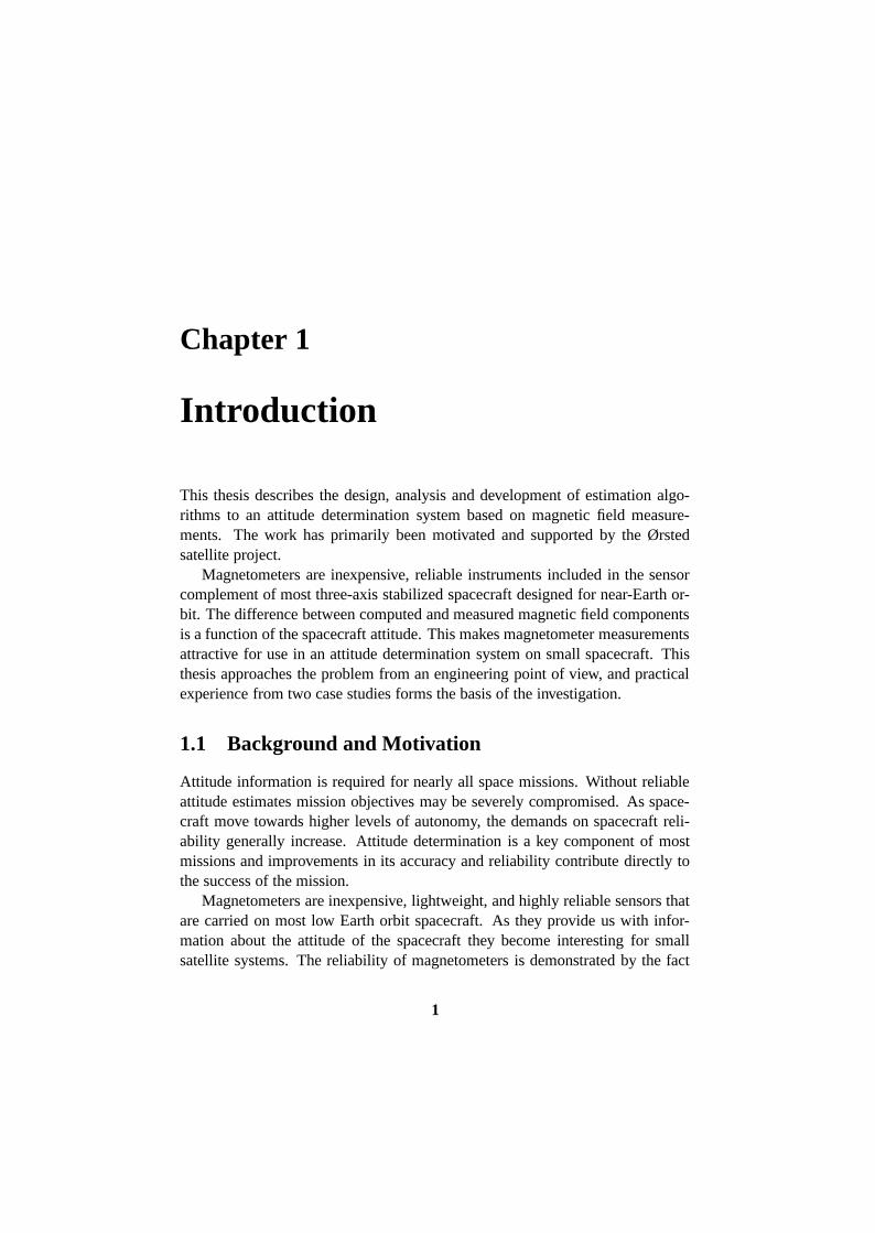
This thesis describes the design, analysis and development of estimation algo-rithms to an attitude determination system based on magnetic field measure-ments. The work has primarily been motivated and supported by the Ørstedsatellite project.
Magnetometers are inexpensive, reliable instruments included in the sensorcomplement of most three-axis stabilized spacecraft designed for near-Earth or-bit. The difference between computed and measured magnetic field componentsis a function of the spacecraft attitude. This makes magnetometer measurementsattractive for use in an attitude determination system on small spacecraft. Thisthesis approaches the problem from an engineering point of view, and practicalexperience from two case studies forms the basis of the investigation.
1.1 Background and Motivation
Attitude information is required for nearly all space missions. Without reliableattitude estimates mission objectives may be severely compromised. As space-craft move towards higher levels of autonomy, the demands on spacecraft reli-ability generally increase. Attitude determination is a key component of mostmissions and improvements in its accuracy and reliability contribute directly tothe success of the mission.
Magnetometers are inexpensive, lightweight, and highly reliable sensors thatare carried on most low Earth orbit spacecraft. As they provide us with infor-mation about the attitude of the spacecraft they become interesting for smallsatellite systems. The reliability of magnetometers is demonstrated by the fact
1
2 Introduction
that, only one failure of a magnetometer has ever been reported on missionssupported by NASA’s Goddard Space Flight Center (Deutchmann et al. (1998)).Another example of the use of magnetometers for attitude determination is givenby the Earth Radiation Budget Satellite (ERBS). In July 1987 ERBS went intoa tumble, which made Sun and Earth sensors unreliable and the gyro telemetrysaturated, so that the three-axis magnetometer became the only useful attitudesensor (Challa et al. (1997)).
The Earth’s magnetic field is primarily a dipole generated largely by currentsin the Earth’s fluid core. The Earth’s magnetic field interacts with and shields usfrom the solar wind. Coronal mass ejections from the Sun cause changes in themagnetosphere shape and local field strength. These fluctuations are the causeof phenomena like the Aroura Borealis and the Van Allen Radiation Belts. Suchperturbations to the main field limit the accuracy of magnetometer based solu-tions. They are, however, still attractive for missions with relative low accuracyrequirements, which require simple inexpensive sensors. Alternatively, missionsdesiring an inexpensive backup method for a more complex attitude and rateestimation packages may use a magnetometer solution.
In 1998 the Gurwin-II Techsat was launched. The platform was stabilizedbased on attitude information from a magnetometer only. The coarse cruisealgorithms has an expected accuracy of 5 deg.. In the fine cruise phase, theuse of an extended Kalman filter is expected to provide an accuracy of 1-2 deg.(Oshman (1999)).
Two case studies have motivated this work, and the results are presented intwo case study chapters.
1.1.1 The Ørsted Case
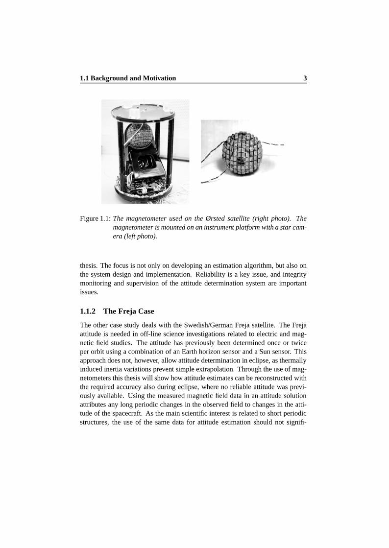
The first case is defined by the Danish Ørsted Satellite. Ørsted is a small satellite,which was launched by a Delta II launch vehicle February 23, 1999. The primaryscience objective is to measure the main geomagnetic field, and a magnetometeris carried as part of the science payload (see Figure 1.1).
For low-budget space experiments like Ørsted we desire to provide as muchdata as possible regarding the dynamics while satisfying severe constraints onthe size, weight, power, and cost of the instrumentation package. Attitude de-termination is therefore based on a gyro-less configuration with a star imageras the primary instrument. Fault tolerance is obtained, through attitude deter-mination based on the science magnetometer as a backup. The backup attitudealgorithm for Ørsted has been a primary motivation for the work presented in this
1.1 Background and Motivation 3
Figure 1.1: The magnetometer used on the Ørsted satellite (right photo). Themagnetometer is mounted on an instrument platform with a star cam-era (left photo).
thesis. The focus is not only on developing an estimation algorithm, but also onthe system design and implementation. Reliability is a key issue, and integritymonitoring and supervision of the attitude determination system are importantissues.
1.1.2 The Freja Case
The other case study deals with the Swedish/German Freja satellite. The Frejaattitude is needed in off-line science investigations related to electric and mag-netic field studies. The attitude has previously been determined once or twiceper orbit using a combination of an Earth horizon sensor and a Sun sensor. Thisapproach does not, however, allow attitude determination in eclipse, as thermallyinduced inertia variations prevent simple extrapolation. Through the use of mag-netometers this thesis will show how attitude estimates can be reconstructed withthe required accuracy also during eclipse, where no reliable attitude was previ-ously available. Using the measured magnetic field data in an attitude solutionattributes any long periodic changes in the observed field to changes in the atti-tude of the spacecraft. As the main scientific interest is related to short periodicstructures, the use of the same data for attitude estimation should not signifi-
4 Introduction
cantly affect the science measurements.
1.1.3 Other Examples
An example of the usefulness of miniature magnetometers may indicate whatthe future will bring in terms of the use of magnetometers for spacecraft atti-tude determination. Researchers at the Jet Propulsion Laboratory have proposeda mission where a single larger satellite ejects several spinning hockey pucksized, disposable, free flying satellites in order to make simultaneous spatiallydistributed measurements. Each pico-sat carry a miniature 3-axis fluxgate mag-netometer and a transmitter. After launch from the main satellite, the picosatstransmit sensor readings back to the main satellite where the data is availablefor retrieval. After the battery discharges completely, the pico satellite dies, andeventually burns up in the atmosphere. The on-board magnetometer supportsthe science objectives, and provides attitude dynamics information for use inevaluation of the science data (Clarke et al. (1996)).
1.2 Overview of Existing Methods
In 1965, Wahba (1965) posed the problem of finding a proper orthogonal (rota-tion) matrix given a number ( ��� ) of vector measurements (see Chapter 2 for amore detailed discussion). Numerous solutions to the problem posed by Wahbahas been proposed over the years (e.g. Lerner (1978), Shuster and Oh (1981),Markley (1993)). These point estimation algorithms do, however, require at leasttwo vector measurements, and therefore fail when only one vector measurement(e.g. magnetometer measurement) is available. The problem is related to observ-ability. A single three-axis magnetometer measurement can give only two-axesworth of attitude information. At any given time point the rotation about thereference vector can not be resolved.
Under the right circumstances the attitude can be determined using measure-ments of a single reference vector (Psiaki et al. (1990)) by using recursive es-timation algorithms and dynamic models. The measurements are processed se-quentially and retain the information content of past measurements, thereby re-ducing the observability problem by temporal fusion with past data. The mostcommonly used technique for attitude estimation is the Kalman filter (Kalman(1960)).
Very few (if any) on-board attitude determination systems have attempted to

1.3 Objectives and Contributions 5
use only magnetometer data to estimate attitude. This is most likely due to theapparent low accuracy of the measurements. The accuracy of a magnetometerbased attitude solution is mainly limited by:
Calibration Magnetometers are inherently nonlinear devices and an accuratein-flight calibration of the magnetometer is required to get to the specifiedaccuracy.
Magnetic cleanliness The spacecraft has to be magnetically clean to minimizedisturbances in the observations and well as disturbances in terms oftorques acting on the spacecraft.
Accurate timing In order to correlate the measurements and the reference fieldvectors, accurate timing of the measurements is needed.
Perturbations to the main field Perturbations to the main field may vary inmagnitude from fractions of a nT to thousands of nT (Langel (1987)).This inaccuracy in the knowledge of the Earth’s field model easily pro-duces errors of 0.4 deg. about each axis.
Furthermore the complexity of spherical harmonics models of the Earth’s mag-netic field as well as the complexity of the attitude estimator, may prevent theuse of magnetometer based attitude solutions.
1.3 Objectives and Contributions
The main contributions of this thesis are as follows:
– The issue of temporal fusion of data is addressed. It is shown how tempo-ral fusion of data may supplement locally unobservable measurement in away such that the system is observable over time.
– It is argued that most practical implementations of estimators require ap-proximations. The quantitative effects of the approximation errors in theprocess and noise statistics are discussed in detail.
– The covariance singularity resulting from the quaternion constraint isdemonstrated and the use of quaternions in the extended Kalman filteraddressed.
6 Introduction
– The role of the quaternion in the Kalman filter update is addressed basedon a power series of an exponential map.
– A significant contribution of this thesis is the complete design, implemen-tation, and test of an attitude determination system for the Ørsted satel-lite. The Ørsted magnetometer based solution solved the initial problemof providing attitude during all mission phases and in case of star cameradropout.
– The demonstration of the Ørsted attitude determination based on resultsfrom on–board attitude determination system. Magnetometer based resultsare compared with star camera attitude as a reference. The magnetome-ter based solution has been used frequently since the start of the Ørstedoperation due to frequent star camera dropout.
– The demonstration of an attitude reconstruction algorithm working flightdata from the Freja spacecraft. The attitude reconstruction algorithmsolved the initial science problem, getting attitude during eclipse to thespecified accuracy. The accuracy was enhanced significantly by detectingand avoiding perturbations to the field model.
– It is demonstrated how a single three-axis magnetometer provides a greatdeal of information when the data are appropriately processed.
While this thesis focuses on the specific problem of magnetometer based atti-tude determination the techniques have much wider potential in the design ofnavigation/attitude estimators.
1.4 Thesis Outline
The thesis is organized as follows:
– Chapter 2, Attitude Determination in Perspective This chapter providesan overview of the diverse field of attitude determination. A brief overviewof attitude sensors most commonly used in attitude determination systemsare given with special emphasis on the measurements obtained from a flux-gate type magnetometer. A brief introduction to deterministic and recur-sive approaches to attitude estimation are provided.
1.4 Thesis Outline 7
– Chapter 3, Attitude and Spacecraft Motion Models This chapter intro-duces a number of attitude representations with the focus on quaternions.An exponential map formulation is presented, which allow an series ex-pansion of the quaternion in terms of ����� skew symmetric matrices.Satellite motion models are derived and the dominant disturbance torquesdescribed.
– Chapter 4, Attitude Estimation This chapter considers estimation basedon extended Kalman filtering. Its structure and operation is described,and the application to nonlinear systems is examined. It is shown howthe Kalman filter predictions allow temporal fusion of the measurementsthereby avoiding a local observability problems, which arise when usingmagnetometers as the only reference sensor. The issue of approximatemodels is also addressed and the effects on the noise statistics quantified.The issue of preserving the norm of the quaternion in the Kalman filteras well as covariance singularity problems related to a full state estimatorare discussed. Finally an attitude estimator solution based on a quaternionvector update is outlined.
– Chapter 5 Ørsted Attitude Estimation The first application, the Ørstedsatellite is described. Two different process models are described and theirnoise statistics discussed in detail. The chapter summarizes and evaluatesthe performance of the two algorithms. An algorithm is selected and fur-ther analyzed, and the predicted performance of the Ørsted attitude algo-rithm is presented.
– Chapter 6 Implementation and Results from Ørsted It is well–knownthat the Kalman filter in its original formulation is sensitive to numericalinaccuracy and potential instability. The numerical behaviour of the algo-rithm is therefore addressed and a brief description of the issues related toa fixed point Ada implementation for Ørsted is given. Finally results fromthe on-board estimator are presented. The results from the magnetome-ter based attitude solution are compared to star camera attitudes therebyproviding an assessment of the absolute accuracy.
– Chapter 7 Freja Attitude Estimation The second application, the Frejasatellite is described. The chapter summarizes and evaluates the perfor-mance of the attitude reconstruction algorithm applied to Freja data. Therequired accuracy and the implications on the estimator design are dis-

8 Introduction
cussed. The solution approach is addressed and reconstruction results arepresented. Periods with disturbed magnetic field measurements are de-tected using a statistical test.
– Chapter 8 Conclusion This chapter gives concluding remarks and recom-mendations for future work.

Chapter 2
Attitude Determination inPerspective
Obtaining accurate attitude information is a fundamental aspect of most spacemissions. Without reliable estimates of the spacecraft attitude, the ability to con-trol the spacecraft and send data back to Earth, or meet other mission objectivesmay be jeopardized.
Sensor information is generally combined in an attitude determination sys-tem to provide the best possible estimates at all times. Depending on the require-ments of the mission, the attitude determination may be performed in real-timeon-board, or alternatively processed in batches on the ground based on informa-tion down-linked from the spacecraft.
Attitude determination systems are a diverse field, but fundamentally theyall require a measurement system that includes sufficient sensors to enable thatattitude information is extracted with the necessary accuracy. Section 2.1 gives abrief overview of attitude sensors most commonly used in attitude determinationsystems. Special emphasis is put on the measurements obtained from a fluxgatetype magnetometer. Section 2.2 introduces different solution approaches thathave been investigated over the last decades.
2.1 Attitude Sensors
This section provides a general overview of present attitude sensor technology.Only salient features are highlighted and the section is intended to be informativerather than complete. It should also be noted, that sensors evolve rapidly, and
9
10 Attitude Determination in Perspective
new more precise and lighter sensors are continuously developed.There are basically two classes of sensors commonly used in attitude deter-
mination systems
– Inertial sensors
– Reference sensors
The two classes of sensors are in most practical implementations used to comple-ment each other in a measurement system. Reference sensors typically providesnoisy vector observations at a low frequency. Rate information from the iner-tial sensor (e.g. gyroscopes) is often fed forward through a state estimator asa prediction to be corrected by observations from the reference sensor, therebycomplementing the reference sensor. Recent advances in reference sensors hasprompted for gyroless attitude determination systems which are very interestingfor inexpensive small satellite missions, such as Ørsted.
2.1.1 Inertial sensors
Inertial sensors consists of sensors that measure rotation and/or translational ac-celeration relative to an inertial frame. The sensors are subject to random driftand bias errors, and as a result, the errors are not bounded. In order to providean absolute attitude, regular updates are performed, based on references such asthe Sun, stars, or the Earth. Traditional inertial reference units are mounted ina multi axis gimbal assembly. While accurate, gimballed units are mechanicallycomplex, heavy, and use more power than the increasingly popular strapdownunits. Strapdown units are typically composed of an orthogonal three-axis set ofinertial angular rate sensors and accelerometers. The inertial sensors are directlymounted (strapdown) to the spacecraft structure. Today, strapdown accuraciescompare to gimballed units (Larson and Wertz (1992)). Strapdown units oftenuse rate gyros which measure only changes in attitude. A number of new solid-state concepts have become available in recent years, such as fiber optic andpiezo electric quartz gyros, resulting in decreased size, weight, and cost. Gyrostypically have a drift rate of down to 0.002 deg./hour.
2.1.2 Reference Sensors
A reference sensor measures the direction of a known vector e.g. the Sun point-ing vector. The vector measurement is a function of spacecraft attitude, making
2.1 Attitude Sensors 11
it attractive for attitude determination. The direction of a known vector is typi-cally measured as (i) all three vector components, or (ii) only a direction (line ofsight). The vector magnetometer is a typical example of the first type, whereassun sensors represent the latter.
One sample from a reference sensor does not provide full attitude informa-tion; a Sun sensor cannot detect any rotation of spacecraft about the Sun vector,for example. Two vector directions, ideally orthogonal are needed for completeattitude information. The uncertainty of a reference sensor is made up of twoparts, the accuracy of the sensor itself and the accuracy of the reference it uses.Stars provide the most accurate sources, with the Sun and Earth being progres-sively less accurate references.
Sun sensors The Sun provides a well defined unambiguous reference vector.Sun sensors are visible light detectors, which measure one or two angles betweentheir mounting base and incident sunlight. Sensors range from analog presencedetectors to digital instruments which measure the sun direction to an accuracydown to one arc-minute.
Sun sensors are popular, accurate and reliable, but require clear fields of view.Since most low-Earth orbits include eclipse periods, the attitude determinationsystem must provide some way of handling the regular loss of Sun reference.Typical sun sensor accuracy range from 0.005 deg. to 4 deg. (Larson and Wertz(1992)).
Star sensors Star sensors can be trackers or scanners, the latter being mainlyused on spinning spacecraft. Charged-Coupled Device (CCD) sensors or ActivePixel Sensors (APS) provides a relatively inexpensive way to image the sky andextract information about stellar locations. Any vehicle motion will show up asa shift of the stars in the field of view.
A star camera measures the elevation of the line of sight to a star as projectedonto mutually perpendicular planes which contain the sensor boresight axis. Thelocations of two or more stars on the sensor, along with their locations in inertialcoordinates are sufficient to determine the attitude of the camera with respectto an inertial frame of reference. The star camera is generally sensitive to largeangular velocities of the spacecraft as this causes a smearing of the star imageson the sensor. Current trends in star sensor technology are treated in Padgett etal. (1997). Typical accuracy range from arc seconds to arc minutes (Larson andWertz (1992)). For the Ørsted mission the star camera was developed and built
12 Attitude Determination in Perspective
by the Department of Automation at the Technical University of Denmark. Theinstrument recognizes star patterns in its field of view in any arbitrary directionusing on-board star databases. The camera is highly intelligent and autonomous,yet lightweight and low power consuming. The star camera on Ørsted has anaccuracy of 5-20 arc seconds ( Liebe (1995), Jørgensen (1995)).
Horizon sensors Horizon sensors are infrared devices that detect the contrastin temperature between space and the Earth’s atmosphere. Some nadir-pointingspacecrafts use a wide field-of-view fixed head sensor, which views the entireEarth disk and centers the spacecraft on it, see Reigber (1996). The direct Earth-relative information obtained from Horizon sensors may simplify on-board pro-cessing on Earth pointing spacecraft. Typical accuracies for systems using hori-zon sensors are 0.1 to 0.25 deg., with some applications approaching 0.03 deg.(Larson and Wertz (1992)).
Global Positioning Sensors A novel use of the Global Positioning System(GPS) or Navstar is to adapt it for use in spacecraft attitude determination (seeMelvin and Hope (1993) and Cohen (1992)). Measurements of carrier phasedifferences of the GPS signal measured by two antennas separated by a baselinefixed in the spacecraft allow the relative range of the two antennas to be deter-mined (except for an integer ambiguity). Reference vectors may be inferred fromthe GPS satellite ephemerides readily available in the receiver. GPS receivers arenow becoming more common on spacecraft for timing and precise orbit deter-mination. Differential carrier receivers are more sophisticated (and expensive)than traditional space receivers, but the benefits from an attitude solution mayvery well make them common over the next decade.
A GPS attitude determination experiment flown on the radar calibration(RADCAL) spacecraft (Lightsey et al. (94)) indicates accuracies of about 0.5 -1.0 deg. for relatively small baselines (< 1 meter). The dominating disturbancein these high precision applications is related to multipath as described by Bakand Bayard (1997). Most efforts have been in the use of GPS for attitude de-termination, but a similar radio frequency system for deep space missions (theautonomous formation flying sensor) was addressed by Bak (1997).
Magnetometers Magnetometers are simple, reliable and lightweight sensorscarried on most spacecraft as part of the attitude control system. The combina-tion of three sensor elements mounted on an orthogonal base make up a vector
2.1 Attitude Sensors 13
sensing system. A three axis magnetometer measure directly the direction andintensity of the local magnetic field expressed in the sensor frame. The use ofmagnetometers for attitude determination is limited to regions with a strong andwell known field, e.g. Low Earth orbits. The attitude is determined from mag-netometer by comparing the measured geomagnetic field with a reference fielddetermined by a reference model.
The accuracy of magnetometers is not as good as that of star or horizon ref-erences due to factors such as:
– Disturbance fields due to spacecraft electronics,
– Model errors in the reference field model,
– External disturbances such as ionospheric currents.
The magnetic field at any location near the Earth can be attributed to a com-bination of sources located respectively in the Earth’s core and crust, and in theEarth’s ionosphere and beyond. By far the largest in magnitude is the field fromthe core, or the main field. Near dipolar in nature, the strength of the main field isapproximately 60.000 nT (nano Tesla) at the poles and approximately 30.000 nTat the equator.
The field model most often used is the International Geomagnetic ReferenceField (IGRF) (Langel (1987)) which is the empirical representation of the Earth’smain magnetic field recommended for scientific use by the International Asso-ciation of Geomagnetism and Aeronomy (IAGA). The IGRF models representthe main field without external sources and they are established as the weightedmean of models developed by a number of agencies. According to Primdahl andJensen (1984) the field is predicted to within approximately 100 nT. A represen-tation of the IGRF field model is given in Figure 2.1. For a discussion of thefield model, see Section B.3.
The temporal variations of the field are slow, with a maximum of about 1%per year. External current systems are time-varying on a scale of seconds up todays, and the resulting near-Earth fields can vary in magnitude from fractions ofa nT to thousands of nT. The external current systems are located in the mag-netosphere, and in the Earth’s ionosphere. The strength and location of thesecurrents vary considerably between magnetically quiet and disturbed times.
The main geomagnetic field has direction as well as magnitude. Given thatthe main field is curl free, allows a representation of � as the gradient of a scalar
14 Attitude Determination in Perspective
Figure 2.1: The reference models of the Earth magnetic field represent the main(core) field without external sources. Magnetic field intensity at theEarth’s surface in ��� based on International Geomagnetic Refer-ence Field (IGRF) model to order 10 for the year 1995.
potential, ��������(� (2.1)
It is, however, known that currents flow within the ionosphere and into and outof the ionosphere along magnetic field lines so that, strictly speaking, Equa-tion (2.1) is not valid in the region above about 95 kilometers, where satellitedata are acquired. If we write
��� �¢¡�£¤�¦¥V£§�©¨ (2.2)
where �ª¡ is from sources strictly internal to the Earth, ��¥ , is from sourcesstrictly external to the region where data are acquired, and �¦¨ is from sources
2.1 Attitude Sensors 15
within the region where data are acquired, then �«¡¬£��¦¥ , can be represented bya scalar potential. In practice, the data used to determine � are selected so asto minimize �¨ and the resulting � is assumed to be a good representation of�ª¡�£§�¦¥ .
External disturbances to the core field, are mainly a problem in the outermagnetosphere and in the polar regions where field aligned currents (Birkelandcurrents) and ionospheric currents produce magnetic fields perpendicular to thecore field (Langel (1987)).
For the Ørsted mission a magnetometer was developed and built by the De-partment of Automation at the Technical University of Denmark. The instrumentis a high performance three axis ringcore fluxgate magnetometer based on a highmu metallic glass sensor. As the Ørsted magnetometer is part of the sciencemission the accuracy is estimated to 0.5 nT peak-to-peak.
The measurements of the fluxgate sensor are based on an excitation of thecore in the sensor by a symmetric current waveform. If no external field ispresent, the core is driven symmetrically into saturation and the magnetic fluxgenerated in the core contains only odd harmonics. If, however, an external fieldis present, the magnetic flux generated in the core will be non-symmetrical andeven harmonics are generated. In a linear sensor the size of the even harmonicsis proportional the external field. A pick-up coil surrounding the excitation coilmakes it possible to measure the generated flux and hence measure the magneticfield by detection the contents of second- or higher even harmonics (see Prim-dahl and Jensen (1984)). The fluxgate ringcore sensor is the preferred design inmodern magnetometer design.
2.1.3 Sensor Summary
The choice of attitude sensors for a specific mission is likely to depend mainly onthe required orientation of the spacecraft and the required accuracy. Other factorsinclude the given financial resources, the requirements to mass, redundancy, faulttolerance, and data rates. Typical performance and physical characteristics aresummarized in Table 2.1.
For full three-axis single point attitude knowledge, at least two reference vec-tor measurements are required. Sensors like GPS and star camera generally pro-vide two or more reference vector measurements at any one time instance.
Frequently, the sensor measurements are made in frames other than the frameof interest for the control system (e.g. local vertical local horizontal (LVLH)),
16 Attitude Determination in Perspective
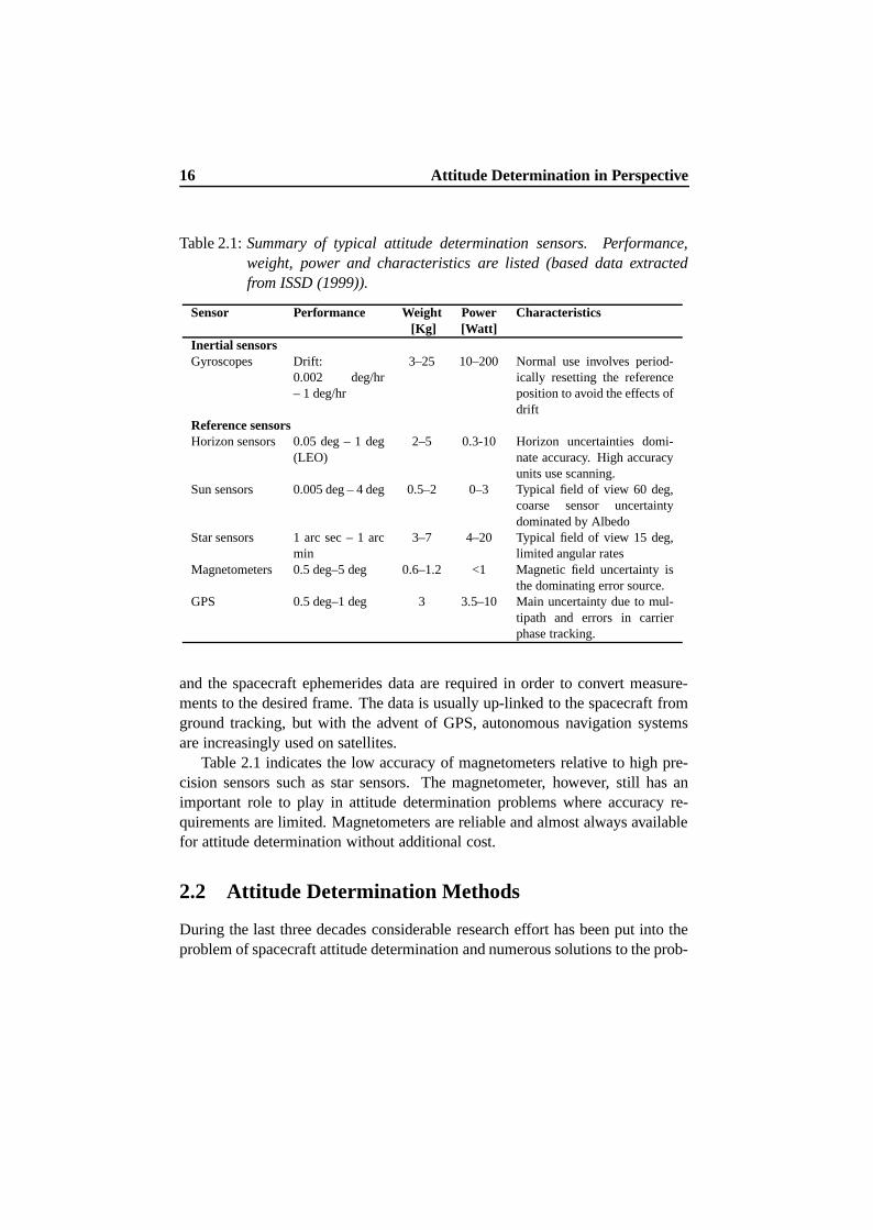
Table 2.1: Summary of typical attitude determination sensors. Performance,weight, power and characteristics are listed (based data extractedfrom ISSD (1999)).
Sensor Performance Weight Power Characteristics[Kg] [Watt]
Inertial sensorsGyroscopes Drift:
0.002 deg/hr– 1 deg/hr
3–25 10–200 Normal use involves period-ically resetting the referenceposition to avoid the effects ofdrift
Reference sensorsHorizon sensors 0.05 deg – 1 deg
(LEO)2–5 0.3-10 Horizon uncertainties domi-
nate accuracy. High accuracyunits use scanning.
Sun sensors 0.005 deg – 4 deg 0.5–2 0–3 Typical field of view 60 deg,coarse sensor uncertaintydominated by Albedo
Star sensors 1 arc sec – 1 arcmin
3–7 4–20 Typical field of view 15 deg,limited angular rates
Magnetometers 0.5 deg–5 deg 0.6–1.2 <1 Magnetic field uncertainty isthe dominating error source.
GPS 0.5 deg–1 deg 3 3.5–10 Main uncertainty due to mul-tipath and errors in carrierphase tracking.
and the spacecraft ephemerides data are required in order to convert measure-ments to the desired frame. The data is usually up-linked to the spacecraft fromground tracking, but with the advent of GPS, autonomous navigation systemsare increasingly used on satellites.
Table 2.1 indicates the low accuracy of magnetometers relative to high pre-cision sensors such as star sensors. The magnetometer, however, still has animportant role to play in attitude determination problems where accuracy re-quirements are limited. Magnetometers are reliable and almost always availablefor attitude determination without additional cost.
2.2 Attitude Determination Methods
During the last three decades considerable research effort has been put into theproblem of spacecraft attitude determination and numerous solutions to the prob-
2.2 Attitude Determination Methods 17
lem have been established. In general the solutions fall into two groups:
– Deterministic (point-by-point) solutions, where the attitude is found basedon two or more vector observations from a single point in time,
– Filters, recursive stochastic estimators that statistically combine measure-ments from several sensors and often dynamic and/or kinematic models inorder to achieve an estimate of the attitude.
2.2.1 Deterministic (point-by-point) solutions
Three-axis point-by-point solutions, that is, solutions that utilize only the vec-tor measurements obtained at a single time point, are widely used in spacecraftapplication.
The TRIAD algorithm (Lerner (1978)) provides a simple deterministic solu-tion for the attitude. The solutions are based on two vector observations given intwo different coordinate systems. TRIAD only accommodates two vector obser-vations at any one time instance. The simplicity of the solution make the TRIADmethod interesting for on-board implementations (see Flatley et al. (1990)). Bar-Itzhack and Harman (1997) has presented an optimized TRIAD algorithm whichprovides a weighted result of two TRIAD solutions which is more accurate thanthe best of the two individual TRIAD solutions that are the basis of the algorithm.
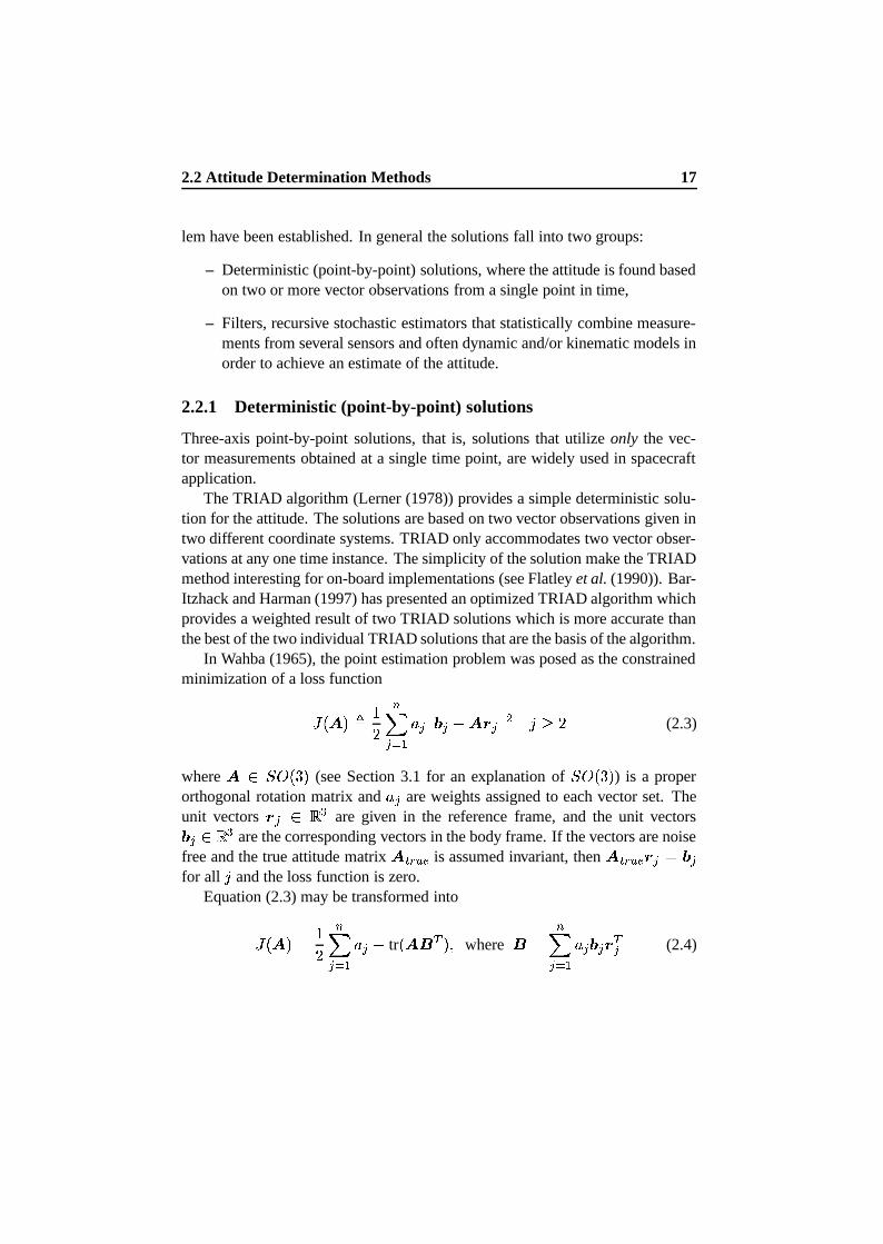
In Wahba (1965), the point estimation problem was posed as the constrainedminimization of a loss function
®°¯²±´³¶µ�·�¸¹¨�º¼»�½ ¨¬¾*¿�¨À�
±(Á ¨�¾Ã Ä3�Å� (2.3)
where±ÇÆ�È°Éʯ²Ë�³
(see Section 3.1 for an explanation ofȶÉ3¯²Ë�³
) is a properorthogonal rotation matrix and ½ ¨ are weights assigned to each vector set. Theunit vectors
Á ¨ ÆÍ̶Îare given in the reference frame, and the unit vectors¿ ¨ Ƣ̶Πare the corresponding vectors in the body frame. If the vectors are noise
free and the true attitude matrix±ÏÑÐWÒ ¥ is assumed invariant, then
±´ÏÑÐWÒ ¥ Á ¨l�Ó¿Ô¨for all Ä and the loss function is zero.
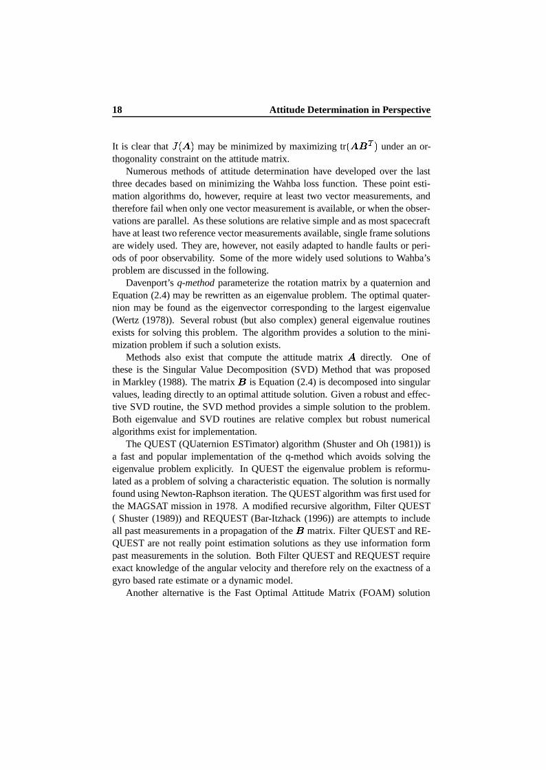
Equation (2.3) may be transformed into
®°¯²±¢³ � ·�¸¹¨�º¼»�½ ¨À� tr
¯²± �´Õ ³*Ö where �×�¸¹¨�º¼»�½ ¨-¿E¨
Á Õ¨ (2.4)
18 Attitude Determination in Perspective
It is clear that®°¯²±¢³
may be minimized by maximizing tr¯²± � Õ ³ under an or-
thogonality constraint on the attitude matrix.Numerous methods of attitude determination have developed over the last
three decades based on minimizing the Wahba loss function. These point esti-mation algorithms do, however, require at least two vector measurements, andtherefore fail when only one vector measurement is available, or when the obser-vations are parallel. As these solutions are relative simple and as most spacecrafthave at least two reference vector measurements available, single frame solutionsare widely used. They are, however, not easily adapted to handle faults or peri-ods of poor observability. Some of the more widely used solutions to Wahba’sproblem are discussed in the following.
Davenport’s q-method parameterize the rotation matrix by a quaternion andEquation (2.4) may be rewritten as an eigenvalue problem. The optimal quater-nion may be found as the eigenvector corresponding to the largest eigenvalue(Wertz (1978)). Several robust (but also complex) general eigenvalue routinesexists for solving this problem. The algorithm provides a solution to the mini-mization problem if such a solution exists.
Methods also exist that compute the attitude matrix±
directly. One ofthese is the Singular Value Decomposition (SVD) Method that was proposedin Markley (1988). The matrix � is Equation (2.4) is decomposed into singularvalues, leading directly to an optimal attitude solution. Given a robust and effec-tive SVD routine, the SVD method provides a simple solution to the problem.Both eigenvalue and SVD routines are relative complex but robust numericalalgorithms exist for implementation.
The QUEST (QUaternion ESTimator) algorithm (Shuster and Oh (1981)) isa fast and popular implementation of the q-method which avoids solving theeigenvalue problem explicitly. In QUEST the eigenvalue problem is reformu-lated as a problem of solving a characteristic equation. The solution is normallyfound using Newton-Raphson iteration. The QUEST algorithm was first used forthe MAGSAT mission in 1978. A modified recursive algorithm, Filter QUEST( Shuster (1989)) and REQUEST (Bar-Itzhack (1996)) are attempts to includeall past measurements in a propagation of the � matrix. Filter QUEST and RE-QUEST are not really point estimation solutions as they use information formpast measurements in the solution. Both Filter QUEST and REQUEST requireexact knowledge of the angular velocity and therefore rely on the exactness of agyro based rate estimate or a dynamic model.
Another alternative is the Fast Optimal Attitude Matrix (FOAM) solution
2.2 Attitude Determination Methods 19
(Markley (1993)), which provides an iterated solution that avoids the explicitsolution of the eigenvalue problem. Instead Newton’s method for solving theeigenvalue problem is employed. In contrast to QUEST, FOAM solves for theattitude matrix directly. The comparison study in Markley (1993) comparethe efficiency of QUEST and FOAM. The efficiency of the two algorithms iscomparable, but FOAM is more robust in some of the cases investigated. Inaddition FOAM has fewer tuning parameters, which is important in practicalimplementations.
All of the solutions above provide relatively efficient point solutions toWahba’s problem. In an attempt to extend the methods to situations with onlyone vector measurement at any given time instance, Challa et al. (1997) pre-sented an approach utilizing batches of magnetometer observations and the timederivative of these as the basis for a TRIAD solution. With unknown angular ve-locity the solution must be supplemented by dynamic equations. The algorithmhas been applied to data from the SAMPEX satellite and the accuracy was foundto be around 5 deg. (Natanson (1993)). The algorithm is sensitive to errors inthe dynamical model and to high spacecraft rates.
The single point estimation algorithms discussed above are summarized inTable 2.2.
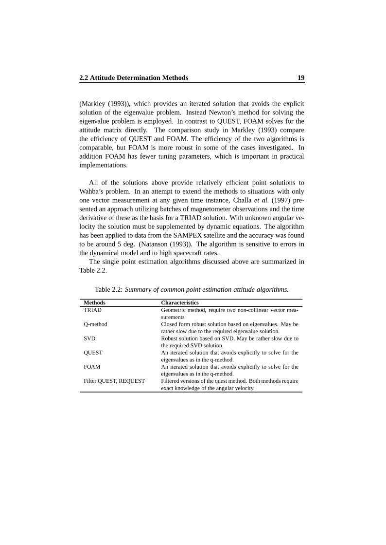
Table 2.2: Summary of common point estimation attitude algorithms.
Methods CharacteristicsTRIAD Geometric method, require two non-collinear vector mea-
surementsQ-method Closed form robust solution based on eigenvalues. May be
rather slow due to the required eigenvalue solution.SVD Robust solution based on SVD. May be rather slow due to
the required SVD solution.QUEST An iterated solution that avoids explicitly to solve for the
eigenvalues as in the q-method.FOAM An iterated solution that avoids explicitly to solve for the
eigenvalues as in the q-method.Filter QUEST, REQUEST Filtered versions of the quest method. Both methods require
exact knowledge of the angular velocity.
20 Attitude Determination in Perspective
2.2.2 Recursive Estimation Algorithms
While many of the above point solutions provide efficient algorithms for on-board implementation, there are a number of shortcomings. First of all, theyall require at least two reference vector measurements. Alternatively they neednoise sensitive temporal derivatives combined with measurements from a singlesensor reading.
Secondly, they do not provide complete state information. Most practical im-plementations of satellite attitude control systems rely on rate estimates, which,in combination with the point estimation algorithms, may be obtained from gy-roscopes. Recent advance in sensor technology and the need for reliable, inex-pensive, and lightweight systems for small satellites, however, call for gyrolessconfigurations.
The third shortcoming is that the point estimation algorithms (filter QUESTand REQUEST exempted) only utilize the vector measurements obtained at asingle time point to determine the attitude at that time point, and thereby infor-mation contained in past measurements is lost. A final shortcoming is that thepoint estimation algorithms do not provide a consistent setting for estimatingstochastic disturbances, biases on gyros etc..
When these shortcomings are undesirable, the increased computational bur-den and complexity, imposed by estimation algorithms, generally has to be ac-cepted. Recursive estimation algorithms for attitude determination have there-fore been investigated intensely.
Kalman Filtering A frequently used technique in attitude estimation is theKalman filter (Kalman (1960)). The Kalman filter utilizes an internal state-spacemodel of the system combined with a statistically model of the error associatedwith the internal model and the measurements. The noise is assumed to be mod-eled by zero-mean Gaussian processes with known covariance. The Kalmanfilter minimizes the trace of the error covariance between the estimated and truestate. The measurements are processed sequentially and retain the informationcontent of past measurements and thereby effectively filter noisy measurements.
Kalman filters in various forms have proved useful for attitude estimation us-ing a combination of reference vectors and gyro measurements (see the surveypaper by Lefferts et al. (1982)). In Bar-Itzhack and Oshman (1985) a variant ofthe Kalman filter was used to estimate the attitude assuming an additive correc-tion.
Under the right circumstances the attitude can be determined without rate
2.3 Summary 21
measurements. This approach has been used in a Real-Time Sequential Filter(RTSF) algorithm which propagates state estimates and error covariances usingdynamic models (Challa (1993)). High bandwidth star tracker measurementswere used in Gai et al. (1985) to drive the estimation of attitude and attituderates. In Fisher et al. (1989) a Kalman filter was designed that takes attitudeinput computed by the QUEST algorithm.
One of the main problems in relation to the Kalman filter is the need foraccurate models, process and measurement models as well as stochastic models.Spacecraft parameters e.g. moments of inertia, external disturbance torques andmomentum wheel dynamics are typically uncertain and the problem has beenaddressed by several authors. In Psiaki et al. (1990) attitude and attitude ratewere determined using only one set of vector measurements. The attitude waspropagated using an accurate dynamic model augmented by external torquesmodeled as a random walk process.
Batch estimators and smoothers based on a Minimum Model Error (MME)approach have recently been proposed by Crassidis and Markley (1997a). Thisapproach requires no a priori statistics on the model error as this is determined aspart of the solution. Another approach was addressed in Crassidis and Markley(1997b), named Predictive Filtering. This approach allows real-time filteringwhile avoiding the Gaussian state noise assumptions of the Kalman filter. Similarto the MME approach, the predictive filter determines the model-error trajectoryas part of the solution.
Nonlinear observers have in recent years received a lot of research interest,see Nijmeijer and Fossen (1999). The main advantage of nonlinear observertheory is that global convergence and stability can be established via Lyapunovtechniques for particular classes of nonlinear systems. A large variety of openproblems concerning nonlinear observers, however, still exist.
2.3 Summary
This chapter addressed the problem of attitude determination. The basis for anyattitude determination is the sensor suite given on the spacecraft. Section 2.1presented a wide range of sensors commonly used in attitude determination sys-tems. Special focus was given to a presentation of the magnetometer. Finally,Section 2.2 briefly introduced a number of point estimation and recursive attitudedetermination techniques developed over the last three decades.

Chapter 3
Attitude and Spacecraft MotionModels
In order to describe the motion of a rigid body in space it is convenient to startwith a description of its possible orientations. Unlike position, orientation isrelatively hard to represent, and a large number of representations are available.This chapter starts by addressing the subject of orthogonal transformations andthe fundamental properties of rotations are outlined. Section 3.2 gives are briefreview of some of the most commonly used representations. Section 3.3 focuseson the quaternion representation which is used throughout this thesis. An ex-ponential map is introduced that will later be applied in approximations of thespacecraft dynamics. Finally, Section 3.4 presents a description of satellite mo-tion models commonly used in attitude estimation.
3.1 Rotations and Orthogonal Matrices
The development of attitude representations can be found in many books on clas-sical mechanics and on attitude control including Hughes (1986), Wertz (1978),and Shuster (1993).
The objective is to describe rotations of a rigid body inÌÀÎ
which has onefixed point but is otherwise free to rotate about any axis through the fixed point.A rigid body is by definition a configuration of points for which the mutualdistances are preserved during movement and a rotation of a rigid body musttherefore preserve distance. Intuitively, rotations must also preserve the naturalorientation of
Ì Î, i.e. right-handed coordinate systems must be transformed into
23
24 Attitude and Spacecraft Motion Models
right-handed coordinate systems.Consider a set of three mutually orthogonal vectors ( ؼ» Ö Ø Â Ö Ø Î ) that are of
unit length fixed in the point Ù of a rigid body. As these three vectors span thevector space
Ì°Îand are linear independent, they form a basis or a coordinate
system. Given three other vectors¯ ØÛÚ » Ö Ø�ÚÂ
Ö Ø�ÚÎ ³ originating at Ù and fixed in thebody. The basic problem of attitude determination is to process vectors repre-sented in these two frames and then solve for the transformation between the twocoordinate systems. This is illustrated in Figure 3.1.
Figure 3.1: The attitude representation problem: Solve for the transformationbetween the reference coordinate system ( Ø<» Ö Ø Â Ö Ø Î ) and the bodyfixed coordinate system defined by the vectors ( Ø�Ú » Ö Ø�ÚÂ
Ö Ø¬ÚÎ ).
Orthogonal transformations are defined as the group of linear invertibletransformations (Jakubczyk and Respondek (1999))
�ÝÜ Ì ÎQÞß Ì Î(3.1)
that preserve the standard scalar product
à ��á Ö ��â´ã¶� à á Ö â¢ã (3.2)
for any á , â ÆäÌ Î. As the standard scalar product1 induces distance in
Ì Î,
orthogonal transformations preserve the distance between any two points. Equa-tion (3.2) also implies that an orthonormal basis remains orthonormal under
1 åÛæ with the standard scalar product, çÑè�é²ê�ë�ìè�íîê defined is in fact an Euclidian space
3.1 Rotations and Orthogonal Matrices 25
transformation. Rotations are now defined as those orthogonal transformationsthat also preserve the orientation of
ÌJÎ.
The body fixed basis vectors¯ Ø Ú » Ö Ø ÚÂ
Ö Ø ÚÎ ³ in Figure 3.1 may now be expressedin the reference frame using coordinates (which is also orthonormal and therebysatisfying the invariance condition in Equation (3.2))
�ïØ Ú¡ �ι¨*º¼» ½ ¡ð¨ Ø ¨
Öòñ � · Ö � ÖÃË (3.3)
The transformation � is therefore uniquely described by theË � Ë rotation matrix± �×óõô°»öô  ô ζ÷ (3.4)
where ô�¨��ùø ½ »p¨Ö½  ¨Ö½ Î ¨�ú Õ are column vectors. As the vectors are orthonormal
the matrix±
satisfies the following conditions
ô Õ ¡ ô�¨û� ü�¡ð¨ Öòñ�Ö Äý� · Ö � ÖÃË (3.5)
where ü�¡ð¨�� · forñ �þÄ Ö and ü�¡ð¨ÿ��� otherwise. These conditions can be
reformulated in the form ± Õ ± ��� (3.6)
where � is the identity matrix. From Equation (3.6) it follows that����� ¯²± Õ ³ ���� ¯²±¢³ � ����� ¯²±´³ Âû� ·and by that
����� ¯²±´³ �� · . Preservation of orientation leads to the followingadditional condition ���� ¯²±´³ � · (3.7)
The space of matrices satisfying Equations (3.6) and (3.7) is called the specialorthogonal group and is denoted by
ȶÉʯ²Ë�³.
Equation (3.5) implies six constraints on±
matrix leaving at most three de-grees of freedom. This means that there are six redundant elements among thenine components of matrix
±. A number of alternative representations are there-
fore frequently used to parameterize the rotation matrix.At the beginning of this section, it was stated that physical rotations intu-
itively would have to preserve distance as well as natural orientation. Using thescalar product on two column vectors á Ö â Æ¢ÌoÎ
à ± á Öñ â´ã¶� ¯²± á ³ Õ ± â � á Õ ± Õ ± â � á Õ âÍ� à á Ö â´ã (3.8)
26 Attitude and Spacecraft Motion Models
it is clear that applying a rotation matrix to a vector does not change its length.In addition, Equation (3.8) says that the angles between vectors does not changeunder rotation. To verify the preservation of orientation the following vectorproduct relation is true
¯Z± á ³ � ¯²± â ³ � ±Ó¯ á«�¢â ³ (3.9)
The basis for a more physical understanding of rotation is Euler’s theoremthat states that: the general displacement of a rigid body with one point fixed isa rotation about an axis through that point (Goldstein (1950)). The concept isillustrated in Figure 3.2. The rotation angle is � , and the axis of rotation is givenby the unit vector in three-dimensional space.
Figure 3.2: The general displacement of a rigid body with one point fixed is arotation ( � ) about an axis ( ) through that point.
With the help of vector algebra it is possible to derive a transformation thatdescribe the rotation in Figure 3.2. The result is the rotation formula (Goldstein(1950))
Á�� ������� ¯ � ³�Á £ ¯ · ������� ¯ � ³t³ � Õ Á ������� ¯ � ³ � Á (3.10)
which transformsÁ
intoÁ �
.Now define the skew symmetric matrix
ø áû� ú µ�� � ��� Î � Â� Î � ��� »���  �î» �
� (3.11)
3.2 Attitude Representations 27
Applied to a vector it yields the same result as the standard vector cross product,i.e. ø á'� ú>â � á �¤â . The transformation in Equation (3.10) may hence bewritten in terms of the rotation matrix defined by
± ¯ �� ³ ������� ¯ � ³ �P£ ¯ · �!����� ¯ � ³t³ � JÕ¢�"����� ¯ � ³ ø ý� ú (3.12)
where the notation± ¯ �� ³ represents the fact that the rotation matrix is parame-
terized in terms of � and .The result in Equation (3.12) may also be expressed in terms of an exponen-
tial map as defined by Chevalley (1946). Any orthonormal matrix± ƤȶÉʯ²Ë�³
may be expressed in terms of a series ofË � Ë skew symmetric matrices defined
in Equation (3.11)
± ¯ �# ³ � ��$&% ¯ ø �� ý� ú ³ �('¹) º+* ·Ù-, ø �� ý� ú ) (3.13)
After some tedious manipulation of the power series, Equation (3.13) may in factbe brought into the form in Equation (3.12).
3.2 Attitude Representations
The problem of parameterizingȶÉ3¯²Ë�³
has been of interest since 1776, whenEuler first showed that
ȶÉʯ²Ë�³only has dimension three (Stuelpnagel (1964)).
Representations involving more than three parameters are therefore subject toconstraints. It was, however, demonstrated by Stuelpnagel (1964) that no three-parameter set can be both global and nonsingular. In order to specify any globalattitude at least four parameters are needed.
The attitude representations most commonly used besides the rotation matrixare vectors of three and four components. Table 3.1 gives a partial list of the mostcommon parameters and provides a quick comparison of the various means ofrepresenting rotations.
The rotation matrix composition follows standard matrix multiplication andrepresents attitude without any singularities. Apart from analytical studies andfor transforming vectors, this representation is little used due to its high dimen-sion and problems in maintaining orthogonality.
The Euler angles, because of their minimum dimension and clear physicalinterpretations are often convenient for describing or analyzing local motion of
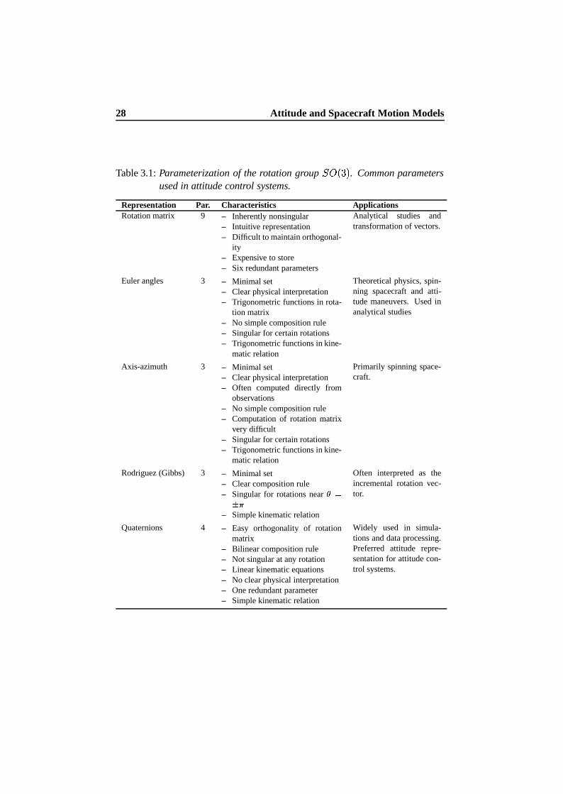
28 Attitude and Spacecraft Motion Models
Table 3.1: Parameterization of the rotation groupȶÉ3¯²Ë�³
. Common parametersused in attitude control systems.
Representation Par. Characteristics ApplicationsRotation matrix 9 – Inherently nonsingular
– Intuitive representation– Difficult to maintain orthogonal-
ity– Expensive to store– Six redundant parameters
Analytical studies andtransformation of vectors.
Euler angles 3 – Minimal set– Clear physical interpretation– Trigonometric functions in rota-
tion matrix– No simple composition rule– Singular for certain rotations– Trigonometric functions in kine-
matic relation
Theoretical physics, spin-ning spacecraft and atti-tude maneuvers. Used inanalytical studies
Axis-azimuth 3 – Minimal set– Clear physical interpretation– Often computed directly from
observations– No simple composition rule– Computation of rotation matrix
very difficult– Singular for certain rotations– Trigonometric functions in kine-
matic relation
Primarily spinning space-craft.
Rodriguez (Gibbs) 3 – Minimal set– Clear composition rule– Singular for rotations near .ýì/10– Simple kinematic relation
Often interpreted as theincremental rotation vec-tor.
Quaternions 4 – Easy orthogonality of rotationmatrix
– Bilinear composition rule– Not singular at any rotation– Linear kinematic equations– No clear physical interpretation– One redundant parameter– Simple kinematic relation
Widely used in simula-tions and data processing.Preferred attitude repre-sentation for attitude con-trol systems.
3.3 Quaternions 29
a body. Nonlinear composition rules and singularities when representing globalattitude limit their usefulness.
The axis-azimuth representation has been used primarily for spinning space-craft as the parameters can often be computed directly from observations. Thisrepresentation is similar to the Euler angles, and experiences many of the sameproblems.
The Rodriguez parameters (Gibbs vector) finds little use and may can be seenas an intermediate step before the quaternion.
The quaternion representation is widely used in simulation, since its kine-matic equations are linear and offer none of the analytical problems (singulari-ties) of representations of smaller dimensions. The parameterization of
ȶÉʯ²Ë�³is
simple as it only involves quadratic terms of the quaternion components, and thequaternion unit norm provides an easy way of maintaining orthogonality of therotation matrix. Composite rotations are expressed in terms of quaternion mul-tiplication. Quaternions are therefore the preferred parameterization for manymodern attitude control systems.
3.3 Quaternions
In this section the representation of rotations in terms of quaternions is discussed.Such a representation is not just concise and elegant but also yields a very ef-ficient way of handling compositions of rotations. The mathematical theory ofquaternions was first developed by Hamilton (1866). Quaternions are also knownas hypercomplex numbers and denoted by 2 . Two different representation ofquaternions are used in this thesis.
First it is convenient to think of quaternions as complex numbers with a scalarreal part, 3 , and a three-dimensional imaginary part, 4 2. Now define a quaternionby 5
��3À£63�»87 £63 Â:9 £63 Î�; (3.14)
where 7 Ö 9 Ö ; are mutually perpendicular unit vectors spanning the space orthog-onal to the real part 3 . For short we write5
� ¯ 3'£<4 ³ (3.15)
2Note that the imaginary part is written in bold italic, whereas the full quaternion is writtenusing upright boldface.
30 Attitude and Spacecraft Motion Models
In fact the real part, 3 , is the projection onto a unit vector Ø in four dimensionalEuclidian space =?> , and the vectors 7 Ö 9 Ö ; are unit vectors in = , the orthogonalcomplement to the vector space spanned by Ø . In this way quaternions are anextension of the imaginary numbers.
The second representation is suitable for applications of matrix algebra.Quaternions are expressed simply as a four-dimensional column vector5
�A@ 43CB (3.16)
A quaternion with a null real part ( 3 �D� ) will be used to represent three di-mensional vector in
ÌoÎ. Likewise, we identify a scalar with a quaternion having
vanishing vector part.Define a left and right operator acting on the quaternion EFHG µ @ Ù1���Åø Il� úJI�KI Õ Ù B and L G µ @ Ù-�l£ ø IP� úMI�NI Õ Ù B (3.17)
The quaternion product operation is then defined asE 5 µ FHG 5 or E 5 µ LPO#E (3.18)
where E Ö 5 Æ 2 and the multiplication on the left hand side is a quaternion prod-uct, whereas the right hand side multiplication is a normal matrix product. It isobvious from Equation (3.18) that the quaternion product rule is only commuta-tive when the vector parts for the two quaternions are parallel so that the crossproduct in Equation (3.18) vanish. However, multiplication by a purely scalarquaternion (
5�Q3'£SR ) is always commutative.
The quaternion conjugate is defined similar to the complex numbers as EUTÀ�¯ Ùw�VI ³ or alternatively in vector notation E T � ø �KI Õ Ù�ú Õ . The quaternion normis defined as
¾WEû¾  � Ù�Ùw£XI Õ I/��E T E (3.19)
which is analogous to the Euclidean vector norm. A unit quaternion is a quater-nion with norm 1, which may be interpreted geometrically as points on the unit3-sphere,
È{Î. The normalization is easily enforced usingE ¸ � ¯ E T E ³WY »[Z Â�E
3.3 Quaternions 31
The remainder of this section will focus on the representation of rotationby the unit quaternion. The symmetric operation on a vector represented as aquaternion with zero real part, \ Æ 2 by\ � � 5 \ 5 T (3.20)
where
5is a unit quaternion defines the orthogonal transformation of the vectorá as represented by the quaternion \ .
By applying successive quaternion product operations (Equation (3.18)), thevector á is transformed into
á � � ¯ 3  ��4 Õ 4 ³ á3£¤�]4 ¯ 4 Õ á ³ � �]3]4 �¢á (3.21)
The correspondence between the quaternion and the rotation matrix±
is there-fore
± ¯5³ � ¯ 3  ��4 Õ 4 ³ �l£¤�]4^4 Õ �ÿ�]3¬ø 4J� ú (3.22)
It is clear that for any quaternion representation of a point inȶÉʯ²Ë�³
,± ¯5³ �± ¯ �
5³, that is, two antipodal points
5and �
5inÈ Î
represents the same rotationinȶÉʯ²Ë�³
.By comparison of the result in Equation (3.22) with the result in Equa-
tion (3.12) it is clear that the quaternion may be expressed as5������� ¯ �&_ � ³ £6����� ¯ �&_ � ³ (3.23)
where is a unit vector representing the axis of rotation, and � is the rotationangle. ����� ¯ �C_ � ³ represents the real part of the quaternion, and ���`� ¯ �&_ � ³ is theimaginary (vector) part. The division by two in the angle of rotation reflects thefact that
5appears twice in Equation (3.20).
Similar to the rotation matrix in Equation (3.13) the quaternion may also beexpressed in terms of an exponential map. Given a rotation by an angle of �]�about the vector , the quaternion exponential is defined as5
¯ � Ö ³ � ��$&% ¯ �# ³ � '¹) º+* ·Ù?, ¯ �� ³ ) (3.24)
where �� on the right hand side is interpreted as a quaternion with zero scalarpart. Note that, as a quaternion product,  � � · . By manipulation of the
32 Attitude and Spacecraft Motion Models
power series, we find��$a% ¯ �� ³ � '¹) º+* ·¯ �*Ù ³ , ¯ �# ³  ) £ '¹) º+* ·¯ �*Ùý£ · ³ , ¯ �� ³  )cb »� '¹) º+* ·¯ �*Ù ³ , ¯ �d�� ³ ) £ '¹) º+* ·¯ �*Ùý£ · ³ , ¯ �e�� ³ ) ¯ �� ³� '¹) º+* ¯ � · ³ )¯ �*Ù ³ , �  ) £f'¹) º+* ¯ � · ³ )¯ �*Ùý£ · ³ , �  )cb » � ����� ¯ � ³ £6�W��� ¯ � ³ (3.25)
This is the same result that was achieved in Equation (3.23). The exponentialmap associated with the attitude matrix was given by a series of
Ë � Ë of skewsymmetric matrices in Equation (3.13). The quaternion map in Equation (3.24) isvery similar in that it represents a series �'�P� skew symmetric matrices when thequaternion product rule is interpreted in terms of Equation (3.18). This under-standing of the quaternions is used in the next section to formulate the kinematicequation for the quaternion.
3.4 Equations of Motion
Thus far, we have examined the general properties of rotations and identifiedseveral possibilities for representing them. The next problem to be addressed isrotations that evolve over time, that is a curve on
È°Éʯ²Ë�³representing the various
orientations. In the following the equations of motion are presented. The kine-matic equations provide the relations between the time derivative of the attituderepresentation and the angular velocity, while the dynamics (or kinetics) describethe development of angular velocities under influence of external moments.
This section makes use of body (principal) and inertial frames. For a detaileddefinition of the coordinate frames see Appendix A.
3.4.1 Attitude Kinematics
Before discussing attitude kinematics the useful concept of infinitesimal rota-tions must be introduced. Infinitesimal rotations are rotations by an infinitesimalsmall angle of rotation, g , about a unit vector, . Using the exponential map
3.4 Equations of Motion 33
from Equation (3.24) the corresponding quaternion is given by5¯ ·� g Ö ³ � · £ ·
� g� �� ·h g  £ji�i�i (3.26)
When composed with a quaternion as
5¯ »Â g Ö ³ 5 the series may be understood
as a sum of quaternion products alternatively as a series of products with skewsymmetric matrices parameterized by the parameters in the sum, and defined bythe composition rule, Equation (3.18). As we will see in the following this isin good agreement with an understanding of the tangent plane being a space of�3�� skew symmetric matrices.
If the attitude is changing with time, then
5¯lk £nm k�³ , the quaternion at timek £<m k , will differ from
5¯lk�³
, the quaternion at timek, and5
¯lk £<m k�³ � 5 ¯ ·� g ¯lk�³*Ö ¯lk�³t³ 5 ¯lkt³ (3.27)
Under the assumption that the rotation is small, the series in Equation (3.26)is truncated to first order, which results in
·m k 5 ¯lk £Sm kt³ � ·m kpo · £ ·� g ¯lkt³ ¯lk�³rq 5 ¯lk�³ £Ss ¯ ¾tgW w¾  ³
� ·m kpo?�P£ ·� @ �dg ¯lkt³ ø ¯lk�³ � úug ¯lk�³ ¯lk�³�dg ¯lk�³ ¯lk�³ Õ � B q 5 ¯lkt³ (3.28)
£vs ¯ ¾tg� w¾ Â ³where the main product in the first line is a quaternion product and the secondline product is the equivalent matrix product.
Defining the angular velocity w ¯lkt³ asw ¯lkt³{µ x ��yz Ï`{ * g ¯lk�³ ¯lkt³m k (3.29)
and taking the limit as m k ß � Equation (3.28) results in|| k 5 ¯lk�³ � ·�~} ¯lk�³ 5 ¯lkt³ (3.30)
where } ¯lk�³ is a skew symmetric �Ê�´� matrix defined as
} ¯lk�³{µ @ �Qø w´� ú�w�ew Õ ��B Ö (3.31)
34 Attitude and Spacecraft Motion Models
These equations are the basis for the integration of attitude. They imply thatif we know the history of the angular velocity w ¯lk�³ , we may integrate and find5¯lk�³
, that is, the attitude history given some initial value of
5¯lk * ³ .
The transformation described by the quaternion above determines the inter-pretation of the angular velocity as defined in Equation (3.29). Given a quater-nion describing the rotation from an inertial to a body frame, the angular velocitywill necessarily be defined in the body frame as the infinitesimal rotation g� isdefined as the rotation from the body frame at time
kto the body frame at timek £<m k .
Using similar reasoning on the rotation matrix leads to the following kine-matic equation || k ± ¯lk�³ ���wø w ¯lk�³ � ú ± ¯lk�³*Ö (3.32)
which is useful when looking at the rate of change of vectors in rotation coordi-nate systems.
3.4.1.1 Differentiation of Rotating Vectors
The rate of change of a vector as seen by two observers in different referenceframes generally differ. Using the product rule for differentiation on á�� ± á �yields | á ¯lkt³| k �
| ±«¯lkt³| k á � ¯lk�³ £ ± ¯lkt³ | á � ¯lkt³| k (3.33)
Applying the result from Equation (3.32), we have| á ¯lk�³| k ����w ¯lkt³ �¢á ¯lkt³ £ ± ¯lk�³ | á � ¯lk�³| k (3.34)
3.4.2 Dynamics
The total system angular momentum � Ú ¯lk�³ÀÆ¦Ì Î of a rigid body with respect toits center of mass is given by (see Kane et al. (1983)):� Ú ¯lk�³ ��� Á Ú ¯lk�³ �¢á Ú ¯lk�³ |�� �Q�dw Ú ¯lkt³*Ö (3.35)
where � Æ«Ì Îc��Î is the moment of inertia matrix of the body about its center ofmass. The vectors
Á Ú and á Ú are the position and velocity of a point mass. Allvectors are given with respect to the body frame as indicated by the subscript � .
3.4 Equations of Motion 35
Suppose the rigid body is subject to external torques. If �"¡ ¯lk�³�Æ«Ì Î denotesthe angular momentum in the inertial frame and �¡ the external torques in theinertial frame, then the momentum balance equation yields|| k��V¡ ¯lk�³ �� "¡ ¯lk�³Using the results from Equation (3.34) this equation is transformed to the bodyframe resulting in || k � Ú ¯lk�³ ����w ¯lk�³ ��� Ú ¯lkt³ £6 Ú ¯lkt³*Ö (3.36)
or � || k�w Ú ¯lk�³ �Ý��w Ú ¯lkt³ � ¯ ��w Ú ¯lk�³t³ £6 Ú ¯lk�³ (3.37)
which is the well–known Euler equation (Goldstein (1950)). The term Ú is thetotal of control and external torques.
3.4.3 External Torques
The torque input in Equation (3.37) is dominated by control torques, aerody-namic drag torques, gravity gradient torques, and torques due to residual mag-netic dipole moments. Apart from control torques which generally are well de-scribed, the latter two dominates in low Earth orbits as seen in Figure 3.3.
For very low orbits the interaction between the aerodynamic drag torques andgravity gradient torques become interesting as described in Bak and Wisniewski(1996) and Bak et al. (1996b).
Control Input and Residual Magnetic Moment The control torque input onØrsted is generated by electromagnetic coils (magnetorquers) and the controlinput torque is hence given by �� ÏÑÐ8� ¯lk�³ ��� ¯lk�³ �ª¿ ¯lkt³ (3.38)
where � ¯lkt³is the magnetic moment generated by current in the torquers, and¿ ¯lkt³ is the local magnetic field in the body frame. A residual magnetic moments
enters into the dynamics in the same way as the control torque, but is not con-trolled actively.
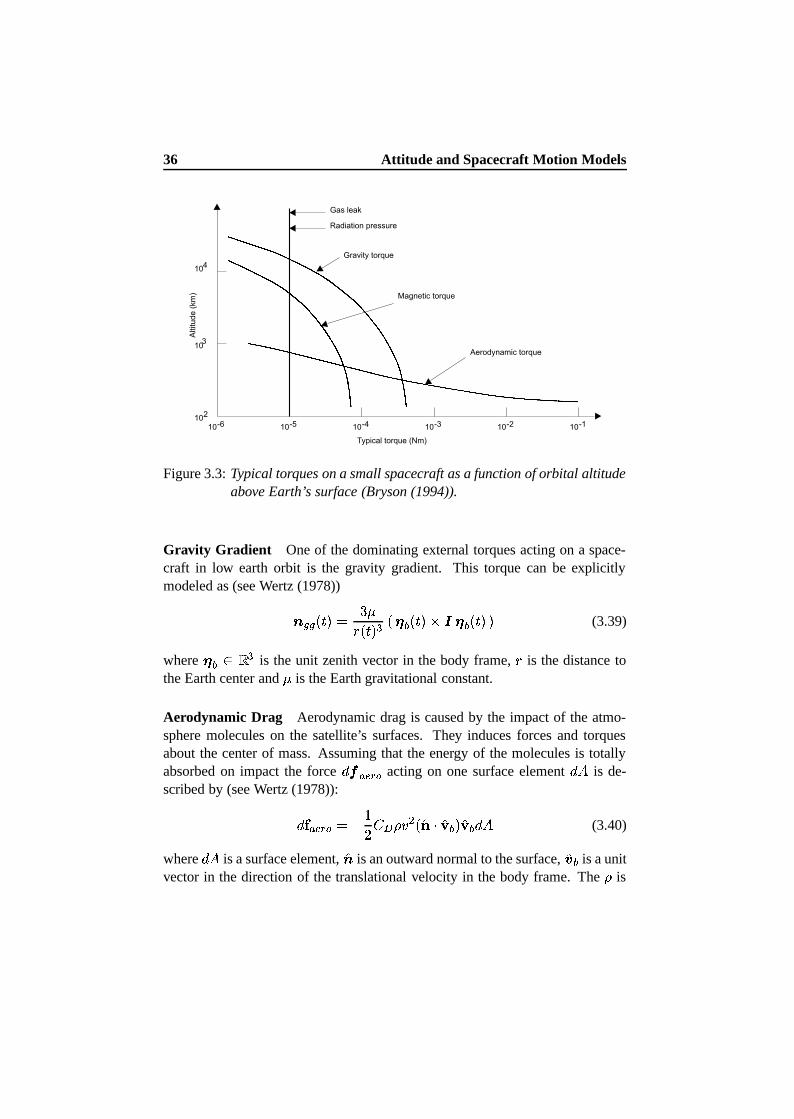
36 Attitude and Spacecraft Motion Models
Figure 3.3: Typical torques on a small spacecraft as a function of orbital altitudeabove Earth’s surface (Bryson (1994)).
Gravity Gradient One of the dominating external torques acting on a space-craft in low earth orbit is the gravity gradient. This torque can be explicitlymodeled as (see Wertz (1978)) U��� ¯lk�³ � Ë��� ¯lk�³ Î ¯]� Ú ¯lk�³ ��� � Ú ¯lk�³�³ (3.39)
where� Ú Æ¤Ì{Î is the unit zenith vector in the body frame, � is the distance to
the Earth center and�
is the Earth gravitational constant.
Aerodynamic Drag Aerodynamic drag is caused by the impact of the atmo-sphere molecules on the satellite’s surfaces. They induces forces and torquesabout the center of mass. Assuming that the energy of the molecules is totallyabsorbed on impact the force
|&�N� ¥ Ð8� acting on one surface element|#�
is de-scribed by (see Wertz (1978)):|#� � ¥ Ð8� ��� ·���U�N� �  ¯c��P� �\ Ú ³��\ Ú |#� (3.40)
where|#�
is a surface element,� is an outward normal to the surface,
�á Ú is a unitvector in the direction of the translational velocity in the body frame. The � is
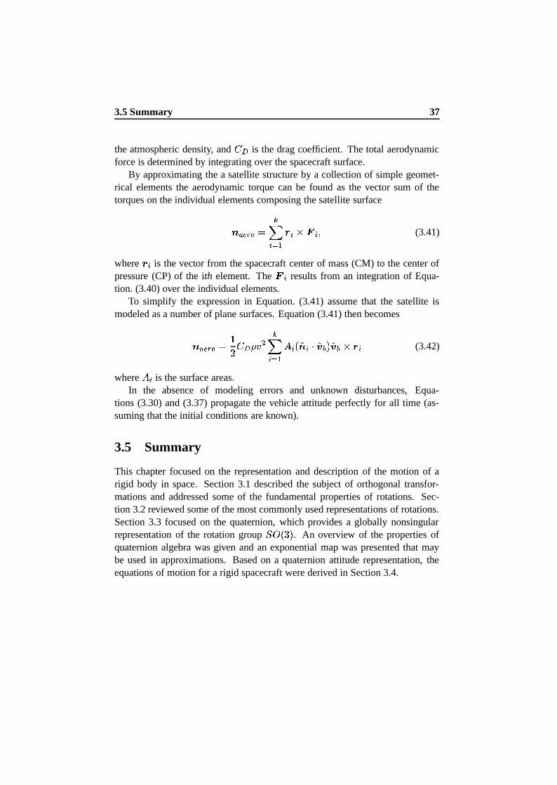
3.5 Summary 37
the atmospheric density, and � � is the drag coefficient. The total aerodynamicforce is determined by integrating over the spacecraft surface.
By approximating the a satellite structure by a collection of simple geomet-rical elements the aerodynamic torque can be found as the vector sum of thetorques on the individual elements composing the satellite surface � ¥ Ð:� � ¹ ¡Nº¼» Á ¡V�P¡ý¡ Ö (3.41)
whereÁ ¡ is the vector from the spacecraft center of mass (CM) to the center of
pressure (CP) of the ith element. The ¡ ¡ results from an integration of Equa-tion. (3.40) over the individual elements.
To simplify the expression in Equation. (3.41) assume that the satellite ismodeled as a number of plane surfaces. Equation (3.41) then becomes � ¥ Ð8� � ·
��� � � ��¢ ¹ ¡Ñº¼» � ¡ ¯ � "¡ � �á Ú ³ �á Ú � Á ¡ (3.42)
where� ¡ is the surface areas.
In the absence of modeling errors and unknown disturbances, Equa-tions (3.30) and (3.37) propagate the vehicle attitude perfectly for all time (as-suming that the initial conditions are known).
3.5 Summary
This chapter focused on the representation and description of the motion of arigid body in space. Section 3.1 described the subject of orthogonal transfor-mations and addressed some of the fundamental properties of rotations. Sec-tion 3.2 reviewed some of the most commonly used representations of rotations.Section 3.3 focused on the quaternion, which provides a globally nonsingularrepresentation of the rotation group
È°Éʯ²Ë�³. An overview of the properties of
quaternion algebra was given and an exponential map was presented that maybe used in approximations. Based on a quaternion attitude representation, theequations of motion for a rigid spacecraft were derived in Section 3.4.

Chapter 4
Attitude Estimation
This chapter considers nonlinear estimation based on Kalman filtering. Attitudedetermination is an estimation problem, and the estimation algorithm determineshow the states are estimated from the sensor information. The attitude determi-nation algorithms in this thesis are based on the Kalman filter. The Kalman filteris based on a structure where predictions made using a model of the system areadjusted using available measurements. This requires accurate models. On theother hand it allows a temporal fusion of data, which is required in order to avoidlocal observability problems when using magnetometers as the only referencesensor.
The basic assumptions behind the Kalman filter are discussed in Section 4.1and Section 4.2 give an overview of the filter structure and operation. The appli-cation of the filter to nonlinear systems is examined in Section 4.3. This leadsto the extended Kalman filter (EKF), which is the most widely used extension ofthe linear Kalman filter to nonlinear problems.
In Section 4.4 the tradeoff between accurate measurements and an accurateprocess model is addressed. It is shown how predictions and observations aretreated equally in the Kalman filter and an approach to model selection is pro-posed. It is argued that most practical estimators require approximations. Thequantitative effects of errors in the process and noise statistics are discussed indetail.
Section 4.6 addresses the issue of preserving the norm of the quaternion inthe Kalman filter as well as covariance singularity problems related to a fullstate estimator. Finally, Section 4.7 presents a quaternion based Kalman filteringsolution, which is later applied in Chapters 5 and 7.
39
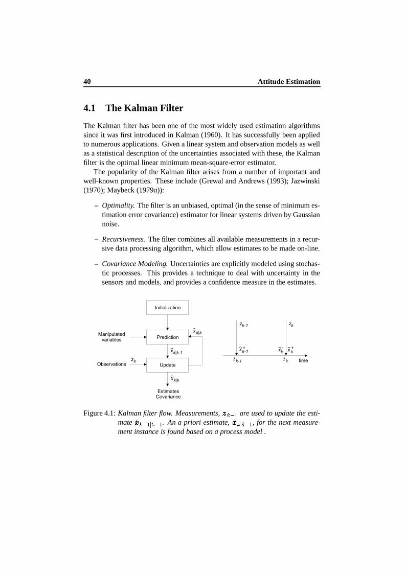
40 Attitude Estimation
4.1 The Kalman Filter
The Kalman filter has been one of the most widely used estimation algorithmssince it was first introduced in Kalman (1960). It has successfully been appliedto numerous applications. Given a linear system and observation models as wellas a statistical description of the uncertainties associated with these, the Kalmanfilter is the optimal linear minimum mean-square-error estimator.
The popularity of the Kalman filter arises from a number of important andwell-known properties. These include (Grewal and Andrews (1993); Jazwinski(1970); Maybeck (1979a)):
– Optimality. The filter is an unbiased, optimal (in the sense of minimum es-timation error covariance) estimator for linear systems driven by Gaussiannoise.
– Recursiveness. The filter combines all available measurements in a recur-sive data processing algorithm, which allow estimates to be made on-line.
– Covariance Modeling. Uncertainties are explicitly modeled using stochas-tic processes. This provides a technique to deal with uncertainty in thesensors and models, and provides a confidence measure in the estimates.
Figure 4.1: Kalman filter flow. Measurements, £ Y » are used to update the esti-mate
�¤ Y »W¥ Y » . An a priori estimate,�¤ ¥ Y » , for the next measure-
ment instance is found based on a process model .
4.1 The Kalman Filter 41
Figure 4.1 shows the basic operation of the filter. It is first initialized— aninitial state of the system and an associated covariance matrix are specified. Thefilter then operates recursively. Each iteration consists of two stages: predictionin time followed by measurement update. With a new measurement at
k Y » , thestate estimate is updated to
�¤ Y »W¥ Y » (the a posteriori estimate). The predictionstage then calculates the a priori estimate for the next sample instance
�¤ ¥ Y » .The prediction is based on a process model describing the evolution of the sys-tem. At time
k a new estimate is formed as a weighted linear combination ofthe a priori state and a correction based on the measurement. The weights arefound such that the mean-squared estimation error is minimized.
4.1.1 Process and Observation Models
The background for the Kalman filter formulation is a state space descriptionof the system. The state of the system at any time
kis expressed using a �
dimensional state space vector ¤ ¯lk�³ . The components of this vector may forexample include the attitude and velocity of the spacecraft, and possibly rele-vant parameters to be estimated. Uncertain parameters include environmentaltorques, components of the inertia tensor for the satellite and possibly sensorcalibration coefficients. The state of the spacecraft changes through time due toits dynamics, which are described using a continuous-time stochastic differentialequation | ¤ ¯lk�³ � � ¯ ¤ ¯lk�³*Ö�¦�¯lk�³*Ö8k�³ | k £ |�§ ¯lk�³ (4.1)
where¦�¯lk�³
is a vector of deterministic control inputs, and§ ¯lkt³
is a Brownianmotion with diffusion ¨ ¯lkt³ . The current time
kis included in the process model
to allow it to be time-varying.This equation may also be written in the less rigorous but for most engineers
more familiar (white noise) notation,|| k ¤ ¯lk�³ � � ¯ ¤ ¯lkt³*Ö�¦P¯lkt³*Ö8k�³ £�á ¯lk�³ (4.2)
where á ¯lk�³ is a vector of stochastic disturbances and contains all perturbations,which act on the system that are not described deterministically by the processmodel. The á ¯lkt³ is assumed to be a zero mean Gaussian noise process withintensity ©«ª
á ¯lkt³W¬ �QR Ö ©«ªá ¯lkt³ á Õ ¯lk £® ³W¬ ��¨ ¯lk�³ ü ¯ ³ (4.3)
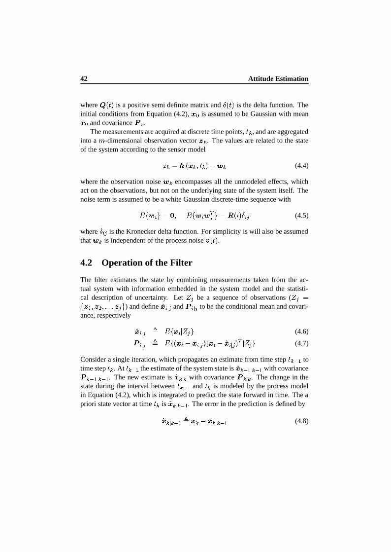
42 Attitude Estimation
where ¨ ¯lkt³ is a positive semi definite matrix and ü ¯lk�³ is the delta function. Theinitial conditions from Equation (4.2), ¤ * is assumed to be Gaussian with mean�¤ * and covariance ¯°* .
The measurements are acquired at discrete time points,k , and are aggregated
into a�
-dimensional observation vector £ . The values are related to the stateof the system according to the sensor model£ �Q� ¯ ¤ Ö8k ³ £ÿâ (4.4)
where the observation noise â encompasses all the unmodeled effects, whichact on the observations, but not on the underlying state of the system itself. Thenoise term is assumed to be a white Gaussian discrete-time sequence with©«ª
â(¡ ¬ ��R Ö ©±ªâ(¡ â Õ¨ ¬ ��² ¯5ñ�³ ü�¡ð¨ (4.5)
where ü ¡ð¨ is the Kronecker delta function. For simplicity is will also be assumedthat â is independent of the process noise á ¯lk�³ .4.2 Operation of the Filter
The filter estimates the state by combining measurements taken from the ac-tual system with information embedded in the system model and the statisti-cal description of uncertainty. Let ³ ¨ be a sequence of observations ( ³ ¨ �ª £V» Ö £ Â Ö i�i�it£�¨ ¬ ) and define
�¤ ¡´¥ ¨ and ¯ ¡´¥ ¨ to be the conditional mean and covari-ance, respectively �¤ ¡´¥ ¨ µ
©«ª ¤ ¡8µ¶³<¨ ¬ (4.6)¯ ¡´¥ ¨ µ©«ª¯ ¤ ¡ � �¤ ¡·¥ ¨ ³�¯ ¤ ¡ � �¤ ¡·¥ ¨ ³ Õ µ¶³ ¨ ¬ (4.7)
Consider a single iteration, which propagates an estimate from time stepk Y » to
time stepk . At
k Y » the estimate of the system state is�¤ Y »W¥ Y » with covariance¯ Y »W¥ Y » . The new estimate is
�¤ ¥ with covariance ¯ ¥ . The change in thestate during the interval between
k Y » andk is modeled by the process model
in Equation (4.2), which is integrated to predict the state forward in time. The apriori state vector at time
k is�¤ ¥ Y » . The error in the prediction is defined by¸¤ ¥ Y » µ ¤ � �¤ ¥ Y » (4.8)
4.2 Operation of the Filter 43
and the covariance of the prediction is¯ ¥ Y » �©«ª ¸¤ ¥ Y » ¸¤ Õ ¥ Y » µ¶³ Y » ¬ (4.9)
The predicted observation is defined by�£ ¥ Y » �©«ª £ µ¶³ Y » ¬ (4.10)
which leads to a definition of the innovation given by¹ µ £ � �£ ¥ Y » (4.11)
and as measurements become available at timek they are incorporated into the
predicted state by finding the weighted sum of the a priori estimate,�¤ ¥ Y » and
the innovation vector, �¤ ¥ � �¤ ¥ Y » £<º ¹ (4.12)
where º is the filter gain matrix (Kalman gain). The error in the observationupdated estimate is ¸¤ ¥ � ¤ � �¤ ¥ � ¤ �¼» �¤ ¥ Y » £Sº ¹ �½ (4.13)
� ¸¤ ¥ Y » �®º ¹ (4.14)
Taking outer products and expectations we get the a posteriori covariance,¯ ¥ �Q¯ ¥ Y » ��¯¿¾ÁÀ º Õ ��º ¯¿À¾ £<º ¯°À�À º Õ (4.15)
where the superscripts on ¯ indicate the cross-covariance matrices.The weighting matrix º , is chosen so that the trace of ¯ ¥ (the mean
squared error) is minimized. The solution was first given by Kalman (1960),º ��¯ ¾ÁÀ ¯ ¯ À�À ³ Y » (4.16)
By using the computed gain in Equation (4.16) we get the Kalman updateequations �¤ ¥ � �¤ ¥ Y » £6º » £ � �£ ¥ Y » ½¯ ¥ � ¯ ¥ Y » �"º ¯ À�À º Õ The covariance prediction from Equation (4.9) determines how informationfrom previous measurements is incorporated into the new estimate.
44 Attitude Estimation
4.2.1 Linear Models
When the system and observation models are linear, there is an exact closed formsolution to the problem. This solution is generally referred to as the Kalman fil-ter. The Kalman filter exists in both continuous, discrete, and continuous/discreteversions. The latter is based on a continuous linear process model and a discreteobservation model || k ¤ ¯lk�³ � ¡ ¯lkt³ ¤ ¯lkt³ £�á ¯lk�³ (4.17)£ � à ¤ £�â (4.18)
The Kalman filter prediction equations are then given by (Maybeck (1979a))|| k �¤ ¯lkt³ � ¡ ¯lk�³#�¤ ¯lk�³ (4.19)|| k ¯ ¯lkt³ � ¡ ¯lk�³ ¯ ¯lk�³ £<¯ ¯lk�³ ¡ Õ ¯lk�³ £<¨ ¯lk�³ (4.20)
The cross-covariances matrices are given by¯ ÀÂÀ � à ¯ ¥ Y » Ã Õ £<² ¯´Ä�³ (4.21)¯ ¾ÁÀ � ¯ ¥ Y » Ã Õ which leads to the familiar observational update equationsº � ¯ ¥ Y » Ã Õ » à ¯ ¥ Y » Ã Õ £S² ¯´Ä�³ ½ Y » (4.22)�¤ ¥ � �¤ ¥ Y » £<º »Å£ �"à �¤ ¥ Y » ½ (4.23)¯ ¥ � ¯ ¥ Y » �"º à ¯ ¥ Y » (4.24)
4.3 Estimators for Nonlinear Systems
For nonlinear systems or non-Gaussian noise, the optimal estimator can only becalculated if the entire density function for the state conditioned on the observedmeasurements is known (Maybeck (1979b)). Since it has no general form, an in-finite number of parameters are required. In practice high order nonlinear filtersare difficult to realize, and virtually all filters, which have been implemented useapproximations of some kind. The simplest and most widely used approach isthe extended Kalman filter (EKF) (Jazwinski (1970)).
4.3 Estimators for Nonlinear Systems 45
4.3.1 The Extended Kalman Filter
The basic assumption behind the EKF is that the process and observation modelsare linear on the scale of the error in the estimated state. By re-linearizationabout each new estimate, the validity of the linearity assumption is less likely tobe violated.
Consider a Taylor series expansion of Equation (4.2) about a nominal trajec-tory defined by ¤ ¸ ¯lk�³Æ¤ ¯lk�³ � Ƥ ¸ ¯lk�³ �ÈÇ � ¯ ¤ ¯lk�³*Ö�¦�¯lk�³*Ö8k�³Ç ¤ ÉÉÉÉ ¤ º ¤~Ê�Ë Ï`Ì ¯ ¤ ¯lk�³ � ¤ ¸ ¯lkt³t³£ h.o.t. £�á ¯lkt³ (4.25)
where “h.o.t.” are terms of powers greater than one in¯ ¤ ¯lkt³ � ¤ ¸ ¯lkt³t³ . The result
is a first order linear approximation to Equation (4.25)|| k�m ¤ ¯lk�³ �Q¡ ¯ ¤ ¸ ¯lk�³*Ö�¦ï¯lk�³*Ö8kt³ m ¤ ¯lkt³ £�á ¯lkt³ (4.26)
where m ¤ is a first order approximation to the state perturbation, and ¡ ¯ � ³ is thematrix of partial derivatives of
� ¯ � ³ with respect to the state (Jacobian matrix),evaluated along the nominal state and input variables. Truncation of the seriesintroduces second and higher-order errors but, by assumption, the effect of thisapproximation is negligible (the strength of á ¯lk�³ may be increased to account forthis assumption).
In a similar way the measurement perturbation model is defined bym±£ ¥ ��à ¯Í�¤ ¥ Ö8k ³ m ¤ ¥ £�â (4.27)
where à ¯ � ³ is the Jacobian of � ¯ � ³ , evaluated along the estimated state.Comparing Equations (4.26) and (4.27) with Equations (4.17) and (4.18), it
is clear that the linear filter is applicable to the linearized system provided theJacobian matrices exist. The output of such a filter would be the optimal estimateof m ¤ ¥ denoted Î m ¤ ¥ . This estimate is combined with the propagated fullstate estimate
�¤ ¥ Y » to establish an estimate of the total state�¤ ¥ � �¤ ¥ Y » £<Îm ¤ ¥ (4.28)
After the incorporation of the estimated perturbation in the full state estimatethe process and measurement models are re-linearized about the new full state.
46 Attitude Estimation
The perturbation Î m ¤ ¥ is reset to zero, and the predicted perturbation Î m ¤ b »W¥ is thus also identically zero.The best estimate of the state between observations is the full state, which is
propagated using the original nonlinear function starting from the initial condi-tion
�¤ ¥ with á ¯lk�³ �Ï� . The new a priori estimate is then used to re-linearizethe filter at time
k b » , which is used in the measurement update equations.The covariance prediction follows the linear Kalman filter covariance prop-
agation in Equation (4.20) based on process and observation models linearizedabout the estimate
�¤ ¥ .Given Î m ¤ b »W¥ �QR , the extended Kalman filters measurement update incor-porates the measurements by means ofÎ m ¤ b »W¥ b » �Qº b » » £ b » �"� ¯ �¤ b »W¥ Ö8k b » ³ ½ (4.29)
where º b » is computed using ¯ b »W¥ and à b » evaluated along the propa-gated full state estimate. The full state is then determined by Equation (4.28).
The basic operation of the EKF is summarized as follows. The filter is sup-plied with initial information, including the measurement error covariance, andestimates of the initial state and associated error. These are used to calculatea gain matrix. The error between the state estimate and the measured data isdetermined and multiplied by the gain matrix to update the state estimate andcovariance. The updated covariance and state are used as input to a nonlinearmodel of the spacecraft dynamics, to predict the projected covariance and stateat the next time instance.
Initially, when the state is only a rough estimate, the gain matrix ensuresthat the measurement data is highly influential in estimating the state. Then, asconfidence in the accuracy of the state grows with each iteration, the gain matrixvalues decrease, causing the influence of the measurement data in updating thestate and associated errors to lessen.
Problems Associated with the EKF The EKF allows us to incorporate nonlin-earities in the filter process and observation models while still exploiting linearestimation techniques. However, there are a number of significant problems withthe EKF
– The assumption that the second and higher order errors might not be neg-ligible and linearization can introduce significant errors. In practice the
4.3 Estimators for Nonlinear Systems 47
inconsistency is often resolved by introducing additional stabilizing noiseterms, which increase the size of the transformed covariance.
– The need to evaluate analytically the Jacobian matrices of the process andobservation models. The Jacobian is not guaranteed to exist and there maybe considerable implementation difficulties when the system is composedof many states and is highly nonlinear.
– The properties of optimality and stability of linear Kalman filters is notguaranteed for EKF. The modeling errors may cause a filter failure modein which the filter covariance estimates become inconsistent, which maylead to filter divergence.
A number of higher order analytical and numerical filters have been devel-oped. Many analytical methods achieve greater accuracy by explicitly includingmore terms in the expansion of Equation (4.25). Second Order Gauss filters(Maybeck (1979b)), for example, assume that the system is locally quadraticand includes both first and second order terms. However, the implementation ofthese filters for even simple systems can be very difficult because it is necessaryto calculate the Hessian as well as the Jacobian. Jazwinski (1970) presents alocal iteration schemes. The measurement state update is iterated until there isno significant change in consecutive iterates. The iterated solution may reducethe effects on the performance of the EKF due to measurement nonlinearities.Higher order filters and iterated solutions are only considered in cases of ex-treme system nonlinearities as they are computational more complex than thestandard EKF.
Numerical methods are able to address both the performance and implemen-tation difficulties. Rather than approximate the model by arbitrary terms in theTaylor Series, they approximate the prior distribution of ¤ Y » by choosing anumber of samples drawn at random. The model is applied to each sample, andthe statistics of the transformed samples are used. One approach is Monte Carlomethods as demonstrated by Handschin (1970). The convergence rates are, how-ever, very slow and a large number of samples are required. In Schei (1997) anew linearization method based on a central point finite-difference approxima-tion was presented. This method avoids explicit evaluation of the Jacobian.
The last problem manifests itself as an inconsistency in the covariance esti-mate ¯ ¡´¥ ¨ � ©«ª ¸¤ ¡´¥ ¨ ¸¤ Õ ¡´¥ ¨ µ¶³ ¨ ¬ÑÐ � (4.30)
48 Attitude Estimation
where ¯ ¡·¥ ¨ is the covariance maintained by the filter, whereas the error vector¸¤ ¡´¥ ¨ is the actual mean-squared error. The inequality in Equation (4.30) is under-stood as a negative definite difference. In other words, the filter believes that itknows the state more accurately than it really does. As a consequence the gainis lower than appropriate. When propagated across over time this may result inan estimation error that becomes progressively worse.
This type of error is often compensated for by modifying the process noise.Increasing ¨ ¯lkt³ will increase the gain, and thereby reduce the effect of modelingerrors. It will, however, increase the sensitivity to errors in the sensor modelingand the sensor noise. Selecting ¨ ¯lkt³ so that the estimated covariance remainshigh, but at the same time low enough to ensure proper filtering is far from easy.The issue is discussed in further detail in Section 4.5.1.
Ljung (1979) discusses the convergence properties of parameter estimationfor linear discrete stochastic systems. An EKF is applied to the problem ofestimating states in a linear system model as well as parameters. The reason fordivergence is shown to be that the effect on the Kalman gain from parameterchanges is not handled properly. Ljung (1979) shows that global convergence ofthe EKF as a parameter estimator may be achieved by including an extra termin the cross coupling between parameters and states. The term included in thecross coupling is the partial derivative of the Kalman gain with respect to theparameters times the innovations. It is also proposed to parameterize the steadystate Kalman gain directly in the filter, rather than the covariance matrices, whichleads to the innovations representation.
In Zhou and Blanke (1989) the innovations representation is extendedto identifying parameters and states of nonlinear state space system models.Second–order terms (bias correction terms) are used in the state expectation andstate predictions in order to allow significant nonlinearities. Both discrete andcontinuous–discrete versions of the algorithm are investigated.
Given these problems with the EKF, it is, however, well–known that extendedKalman filters can be made to operate properly in many practical systems.
4.4 Temporal Fusion of Data
The process model is used to predict the future state of the system. Using the pro-cess model the prediction summarizes all the previous observation information.
4.4 Temporal Fusion of Data 49
The estimate atk is thus not restricted to using the information contained in £ .The prediction allow temporal fusion with data from all past measurements.
The temporal fusion of data is best appreciated by considering the informa-tion form (Maybeck (1979a)) of the prediction. The amount of informationmaintained in an estimate
�¤ is defined to be the inverse of its covariance ma-trix. The covariance prediction in Equation (4.24) may be rewritten as¯ ¥ � ¯ ¥ Y » �"º à ¯ ¥ Y » (4.31)¯ ¥ ¯ Y » ¥ Y » � ���"º à (4.32)
Using this result in combination with the Kalman gain in terms of the predictedcovariance, (Maybeck (1979a))º �Q¯ ¥ Ã Õ ² ¯´Ä�³WY » (4.33)
the state measurement update may be written as�¤ ¥ ��¯ ¥ ÓÒ ¯ Y » ¥ Y » �¤ ¥ Y » £<Ã Õ ² ¯´Ä�³ Y » £ cÔ (4.34)
A similar expression can be found for the predicted information matrix¯ Y » ¥ �Q¯ Y » ¥ Y » £SÃ Õ ² ¯´Ä�³WY » à (4.35)
The estimate in Equation (4.34) is therefore a weighted average of the predic-tion and the observation. Intuitively the weights must be inversely proportionalto their respective covariances. Seen in the light of Equation (4.34) predictionsand observations are treated equally by the Kalman filter. It is therefore possibleto consider the prediction as an observation,
�¤ ¥ Y » with covariance ¯ Y » ¥ Y » .Since the prediction and the observation are equivalent, there is a tradeoffbetween the propagation model and the sensors. The importance of the tempo-ral fusion is demonstrated by the problem of observability in the magnetometersituation. Although the system is not observable about the magnetic field mea-surements at any single point in time the filter is able to estimate the orientationof the spacecraft due to an accurate prediction of the system state.
4.4.1 Information Flow
Theoretically the Kalman filter forms its estimates from the total amount of col-lected observation information, ³ . As the state of the system evolves over time
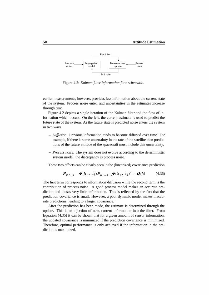
50 Attitude Estimation
Figure 4.2: Kalman filter information flow schematic.
earlier measurements, however, provides less information about the current stateof the system. Process noise enter, and uncertainties in the estimates increasethrough time.
Figure 4.2 depicts a single iteration of the Kalman filter and the flow of in-formation which occurs. On the left, the current estimate is used to predict thefuture state of the system. As the future state is predicted noise enters the systemin two ways
– Diffusion. Previous information tends to become diffused over time. Forexample, if there is some uncertainty in the rate of the satellite then predic-tions of the future attitude of the spacecraft must include this uncertainty.
– Process noise. The system does not evolve according to the deterministicsystem model, the discrepancy is process noise.
These two effects can be clearly seen in the (linearized) covariance prediction¯ ¥ Y » �jÕ ¯lk b » Ö8k ³ ¯ Y »W¥ Y » Õ ¯lk b » Ö8k ³ Õ £<¨ ¯´Ä�³ (4.36)
The first term corresponds to information diffusion while the second term is thecontribution of process noise. A good process model makes an accurate pre-diction and looses very little information. This is reflected by the fact that theprediction covariance is small. However, a poor dynamic model makes inaccu-rate predictions, leading to a larger covariance.
After the prediction has been made, the estimate is determined through theupdate. This is an injection of new, current information into the filter. FromEquation (4.35) it can be shown that for a given amount of sensor information,the updated covariance is minimized if the prediction covariance is minimized.Therefore, optimal performance is only achieved if the information in the pre-diction is maximized.
4.5 Model Selection 51
4.5 Model Selection
The analysis in the previous section shows that the dynamic model should bechosen to maximize the information in the prediction. Intuitively it must closelyapproximate the way that the true system behaves. The order of the true systemis, however, generally high and the system may sometimes not be described bya finite dimension.
The true system takes account of all the effects, which act on the spacecraft.These include states, which are directly relevant to attitude determination (suchas attitude and angular velocity), states, which are indirectly related (for exam-ple, changing atmospheric density) and states, which have only a very slightrelevance (for example, vibration modes in the boom).
Even if the dynamic model were perfectly known and could be describedwith sufficiently few states that it could be implemented, there is an additionalproblem, known as the bias/variance tradeoff. As a model becomes more com-plex, it becomes a better description of the true system, and the bias becomesprogressively smaller. However, a more complex model includes more states.Given that there is only a finite amount of noisy data, the result is that the infor-mation has to be spread between the states and the variance on the estimates ofall of the states increase.
These problems mean that the core issue in designing an attitude estimatoris to find a suitable balance between a detailed dynamic model and an accuratesensor suite. The guiding principle is that the dynamic model should be the leastcomplex model (parsimonious (Ljung (1987))), which is capable of describingthe most significant features of the true system .
4.5.1 Modeling Errors
As mentioned above most practical estimators cannot use a model which de-scribes the true system precisely. Approximations must be made in order toachieve a computational efficient algorithm. This section analyze the problem ofapproximate system models in greater detail and the effects of modeling errorsis quantified. The effect of an approximate system model in the covariance pre-diction context is first analyzed and next the effect of incorrect noise statistics isexamined.
52 Attitude Estimation
4.5.1.1 Covariance Prediction
As discussed in Section 4.3.1 modeling errors are often compensated for in theEKF by increasing the process noise, ¨ ¯lk�³ . The objective in the following is toset up a bound on the minimum value of the process noise that takes modelingerrors into account.
For simplicity, we assume that the process noise is additive and that thereis no control input. The true system then evolves according to the stochasticdifferential equation | ¤ Õ ¯lkt³ � � Õ ¯ ¤ Õ ¯lk�³t³ | k £ |�§ Õ ¯lk�³ (4.37)
where ¤ Õ ¯lk�³ is the state of the true system,|�§Õ¯lk�³
is the process noise, and�Õ¯ � ³ is the true system model.Given the true state vector at time
k , ¤ Õ ¯lk ³ . The true system may be ofhigh order, and approximations are therefore made in the estimator design. It isassumed that there is a structural relationship between the states of the approxi-mate system and the true system given by the projection of the true system state¤ Õ ¯lk ³ onto the approximate system state spaceÖ¤ ¯lk ³¶µØ×°¯ ¤ Õ ¯lk ³t³ (4.38)
whereÖ¤ ¯lk ³ is the projection of the true state onto the approximate state space.
The projection into the approximate state space,Ö¤ ¯lk ³ represents the true system,
but in approximate state space. In the case of zero estimation error,Ö¤ ¯lk ³ would
be our estimate of the true state. The dimension of the approximate systemstate space may be smaller than the dimension of the true state space. In theanalysis here,
×°¯ � ³ need not be explicitly defined unless exact optimum resultsare required.
The actual prediction error of the approximate system at timek is then given
by ¸¤ ¯lk ³{µ Ö¤ ¯lk ³ � �¤ ¥ Y » (4.39)
and the actual mean-squared error prediction error is thus given byÖ¯ ¥ Y » �©±ª ¸¤ ¯lk ³]¸¤ Õ ¯lk ³ µ¶³ Y » ¬ (4.40)
To ensure consistency of the estimator, the process noise parameters ¨ must beselected such that ¯ ¥ Y » � Ö¯ ¥ Y » (4.41)
4.5 Model Selection 53
which means that the predicted error estimate is larger than the actual error.Based on Equation (4.37) the projection of the true system is governed by the
stochastic differential equation| Ö¤ ¯lkt³ ��Ù ¯lkt³ � Õ ¯ ¤ Õ ¯lkt³t³ | k £SÙ ¯lkt³ |�§ Õ ¯lkt³ (4.42)
where the Ù ¯lk�³ and Ù ¯lk�³ is the Jacobian of×°¯ � ³ with respect to ¤ Õ ¯lk�³ . The
model�Õ¯ � ³ describe the evolution of the true system, and
|�§Õ¯lkt³
is the trueadditive process noise.
The first term in Equation (4.42) describe the evolution of the true systemstate without noise, which is projected onto the approximate system space. It isassumed that this may also be written as the evolution of
Ö¤ ¯lkt³ using the approx-imate dynamics and an additive modeling error term, which is a function of thetrue state | Ö¤ ¯lk�³ � � ¯ Ö¤ ¯lkt³t³ | k £SÙ ¯lk�³ |�§ Õ ¯lkt³ £<Ú ¯ ¤ Õ ¯lkt³t³ | k (4.43)
where Ú ¯ ¤ Õ ¯lkt³t³ is the modeling error, which describes the error committed byassuming the approximate dynamicsÚ ¯ ¤ Õ ¯lk�³t³ | k ��Ù ¯lkt³ � Õ ¯ ¤ Õ ¯lkt³t³ | k � � ¯ Ö¤ ¯lk�³t³ | k (4.44)
The estimate and error states are now substituted into Equation (4.43), whichis then linearized about the estimated system state| Ö¤ ¯lk�³ � � ¯��¤ ¯lkt³ £ ¸¤ ¯lkt³t³ | k £SÙ ¯lk�³ |�§ Õ ¯lkt³ £SÚ ¯ ¤ Õ ¯lkt³t³ | k (4.45)Û � ¯ �¤ ¯lkt³t³ | k £<¡ ¯lk�³ ¸¤ ¯lk�³ | k £SÙ ¯lk�³ |�§ Õ ¯lkt³ £<Ú ¯ ¤ Õ ¯lkt³t³ | kwhere ¡ ¯lk�³ is the Jacobian of the approximate dynamics evaluated at the stateestimate
�¤ ¯lk�³ . The evolution of the estimated state is controlled by| �¤ ¯lk�³ � � ¯ �¤ ¯lkt³t³ | kSubtracting the estimated dynamics from Equation (4.45) results in the fol-
lowing error dynamics| ¸¤ ¯lkt³ ��¡ ¯lk�³ ¸¤ ¯lkt³ | k £<Ù ¯lkt³ |�§ Õ ¯lkt³ £SÚ ¯ ¤ Õ ¯lk�³t³ | k (4.46)
The first term in Equation (4.46) accounts for the propagation of estimationerror whereas the second term describe the process noise. These two terms are
54 Attitude Estimation
explicitly maintained by the Kalman filter. The third term is an additional errorintroduced by the approximate system modeling.
In order to arrive at a discrete covariance propagation, Equation (4.46) isintegrated over the interval from
k tok b »¸¤ ¯lk b » ³ �jÕ ¯lk b » Ö8k ³ ¸¤ ¯lk ³ £�á Õ ¯´Ä £ · ³ £SÚ b » (4.47)
where Õ ¯lk b » Ö8k ³ is the state transition matrix. The á Õ ¯´Ä £ · ³ is the true discreteprocess noise projected onto the approximate space and given by
á Õ ¯´Ä £ · ³ ��� Ï`Ü:ÝaÞÏ`Ü Õ ¯lk b » Ö ³ Ù ¯ ³ |�§ Õ ¯ ³The Ú b » is the contribution from the modeling error and defined byÚ b » � �
Ï`Ü:ÝaÞÏ`Ü Õ ¯lk b » Ö ³ Ú ¯ ¤ Õ ¯ ³t³ |
The prediction covariance in Equation (4.40) is now found by taking outerproducts and expectations of Equation (4.47)Ö¯ b »W¥ � Õ ¯lk b » Ö8k ³ Ö¯ ¥ ÕPÕ ¯lk b » Ö8k ³ £<¨ Õ ¯´Ä�³£ßÕ ¯lk b » Ö8k ³ ¯ ¾Áà ¥ £ ¯ ¯ ¾Áà ¥ ³ Õ Õ Õ ¯lk b » Ö8k ³ £S¯ à�à (4.48)
The first two terms are well known from the Kalman filter covariance prediction.The last three terms are cross correlation terms that are included as a conse-quence of modeling errors. The ¯ ¾Áà ¥ is the correlation between the error in thea posteriori state estimate and the modeling error introduced by predicting fromk to
k b » . The last covariance term is ¯ à�à , which is the mean squared value ofthe modeling error term. In case of a very inaccurate approximate model ¯ à^à may not be finite and the process noise is thus unbounded.
The analysis above leads to the following condition on the selection of theprocess noise parameters¨ ¯´Ä�³ � ¨ Õ ¯´Ä�³ £6Õ ¯lk b » Ö8k ³ ¯ ¾Áà ¥ £ ¯ ¯¿¾Áà ¥ ³ Õ Õ Õ ¯lk b » Ö8k ³ £S¯¿à�à á k (4.49)
This analysis has shown that using an approximate system model introduces aperformance penalty. Modeling errors introduce discrepancies in the covarianceprediction, which must be compensated for by increasing the process noise inorder to ensure a consistent estimate. The minimum value of noise is given byEquation (4.49). In most practical systems the actual noise and the modelingerror function are not known and the selection of ¨ ¯´Ä�³ is not trivial.
4.5 Model Selection 55
4.5.1.2 Covariance Update
The observational update in the Kalman filter is based on the innovation, whichrepresented in terms of the true state is given by¹ �Q� Õ ¯ ¤ Õ ¯lk ³*Ö8k ³ £�â Õ ¯´Ä�³ �"� ¯ �¤ ¥ Y » Ö8k ³ (4.50)
Assuming that there are no structural errors in � ¯ � ³ , the true observation is lin-earized about the estimated state� Õ ¯ ¤ Õ ¯lk ³*Ö8k ³ �Q� ¯��¤ ¥ Y » Ö8k ³ £6à ¸¤ ¥ Y » (4.51)
where à is the Jacobian of � ¯ � ³ evaluated at�¤ ¥ Y » .Substituting this result into Equation (4.50) and applying the Kalman obser-
vational update (Equation (4.23)) to the error state we get¸¤ ¥ � ¤ Õ ¯lk ³ � �¤ ¥ � ¤ Õ ¯lk ³ �¼» �¤ ¥ Y » £<º ¹ ͽ� ¯ ����º à ³~¸¤ ¥ Y » £<º â Õ ¯´Ä�³ (4.52)
Taking outer products and expectations, the true mean squared error of the esti-mate is Ö¯ ¥ � ¯ ���"º à ³ Ö¯ ¥ Y » ¯ ���"º à ³ Õ£<º ² Õ ¯´Ä�³ º Õ (4.53)
which is similar the Joseph form (Bucy and Joseph (1968)) of the normal Kalmanfilter covariance update. In the approximate filter knowledge about the true co-variance
Ö¯ ¥ Y » or observation noise ² Õ ¯´Ä�³ is not available, and the update ishence given by¯ ¥ � ¯ ���®º à ³ ¯ ¥ Y » ¯ �Q�"º à ³ Õ £<º ² ¯´Ä�³ º Õ fá k (4.54)
Subtracting Equation (4.54) from Equation (4.53) leads to¯ ¥ � Ö¯ ¥ � ¯ ���"º à ³b¯ ¯ ¥ Y » � Ö¯ ¥ Y » ³�¯ ���"º à ³ Õ£6º ¯ ² ¯´Ä�³ �®² Õ ¯´Ä�³t³ º Õ (4.55)
and in order to ensure consistency we require that ¯ ¥ � Ö¯ ¥ �âR . A suffi-cient condition to ensure that the difference is positive semi definite is (Jazwinski(1970)) ¯ ¥ Y » � Ö¯ ¥ Y » �nR and ² ¯´Ä�³ �"² Õ ¯´Ä�³ �nR á k (4.56)

56 Attitude Estimation
The two conditions state that both the covariance prediction and the observa-tion noise statistics must be consistent. The modeling errors associated with thecovariance prediction must be compensated for by increasing the process noise.A bound on the process noise was established (Equation (4.49)) but it was arguedthat in most practical systems the bound cannot be calculated. The second con-dition in Equation (4.56) states that the approximate systems observation noisemust exceed the noise of the true system.
4.6 The Quaternion in the Kalman Filter
In Chapter 3 the use of quaternions to represent a rotation inÈ°Éʯ²Ë�³
was outlined.The quaternion was chosen as the attitude representation on the Ørsted satel-
lite. The main reasons being the nonsigularity of the representation, the easilyenforced orthogonality (by preserving unit norm), which is important from animplementational point of view, and finally properties that make it ideal for con-troller design (see Wisniewski (1997)).
Before applying the EKF to the attitude estimation problem two problemsmust be addressed. Both are related to the quaternion state
– Covariance Singularity. The unit norm constraint on the quaternion leadsto a constrained error vector, and the associated covariance matrix is there-fore singular.
– Quaternion unity. The filter should preserve the unit norm of the attitudequaternion in order to maintain orthogonality in the rotation. The standardEKF update is based on unconstrained additive corrections, and the resultis not an attitude quaternion as the quaternion has no group structure underaddition.
In the following, alternative forms of the EKF are presented that are norm pre-serving within a linear approximation and numerical round-off, while avoidingthe covariance singularity issue.
4.6.1 Covariance Singularity
As discussed previously, the Kalman filter is designed to minimize the trace ofthe error covariance. That is, suppose
�5is some estimate of the quaternion, and
5is the true attitude. The goal of the Kalman filter algorithms is then to minimize
4.6 The Quaternion in the Kalman Filter 57
the trace of the covariance matrix for the quaternion state, ¯äã:ã , which is definedas a �3�´� matrix ¯ ã:ã � ©±ª ¯Â¸4©� ©±ª ¸4 ¬E³b¯t¸4©� ©«ª ¸4 ¬E³ Õ ¬ (4.57)
where¸4 is the difference between true and estimated attitude¸4 µ 5 � �5 (4.58)
Assuming that the true quaternion is in a small neighborhood of the estimatedquaternion, Equation (4.58) may be rewritten using the exponential power seriesin terms of the rotation vector,¸4´�åo · £ ·
� g� �� ·h g�°£ni�i�i q �5 � �5� o ·� g� �� ·h g  £ji�i�i q �5 (4.59)
and with the definition in Equation (3.18)¸4��LSæO @ »Â gW ��B £Ss ¯ ¾tgW w¾Ã ³ (4.60)
With
©±ª gW ¬ �MR the full quaternion covariance may to first order be approxi-mated by ¯¿ã:ã Û ·
�© o�LSæOç@ g� �HB ó gW Õ � ÷ L´Õ æO q (4.61)Û ·� LSæO @ ¯¿è·è�RR Õ ��B L´Õ æO (4.62)
where ¯ è·è � ©«ªÍé�éÕ ¬ is the attitude error covariance. It follows immediately
that the �l� � covariance matrix is singular. Preserving this singularity is numer-ically difficult and may lead to a inconsistent filter solutions and divergence. Inorder to preserve the singularity it hence necessary to take the normalization con-straint into account explicitly, or reduce the problem to one of lower dimension(i.e. three).
The former approach is generally difficult as the operations performed in thestandard EKF assume independent state variables and therefore do not preservethe unit norm. Several authors (Bar-Itzhack and Oshman (1985); Bar-Itzhack
58 Attitude Estimation
et al. (1991)) have, however, performed numerical investigations and achievedgood results by basically ignoring the constraint on the quaternion and usingthe standard EKF unconstrained update equations on all four quaternion compo-nents.
Lefferts et al. (1982) suggested deleting one of the quaternion components inthe state error vector (the component with largest magnitude) in order to achievea truncated covariance matrix. This approach maintains proper rank of the co-variance matrix and quaternion unity, but the full state transition matrix still hasto be computed each time.
Alternatively Lefferts et al. (1982) suggests a more efficient algorithm basedon a body referenced quaternion correction. Defining the error quaternion as thecorrection that has to be composed with the estimated quaternion in order to getthe true state the error state dimension may be reduced.
Using the exponential map from Equation (3.24) we may parameterize aneighborhood of
�5by 5
� ��$&% ¯ ·� �� ³ �5
� o · £ ·� gW �� ·h g  £�i�i�i q �5 (4.63)
Assuming that the exponential correction in Equation (4.63) is small andtruncating the series to first order we get5 Û o · £ ·
� gW q �5 (4.64)
The estimated quaternion�5
represents the rotation from the reference frame tothe estimated body frame. The correction in Equation (4.64) then represents arotation from the estimated to the true body frame. This is in fact equivalent tothe body referenced correction described in Lefferts et al. (1982).
The truncated series corresponds to a quaternion with unit real part and threefree variables. The basic idea is now only to estimate the three free variables,which are aggregated into a 3 vector such that m«4ª� »Â g� . The error state to beestimated is then given by Î m ¤ ¥ �Èêaëm±4 ¥ ëm±ì ¥
í(4.65)
One independent parameter has been removed from the error state. If ì hasdimension � , then the state error vector has dimension
¯ �P£ Ë�³ , whereas the state
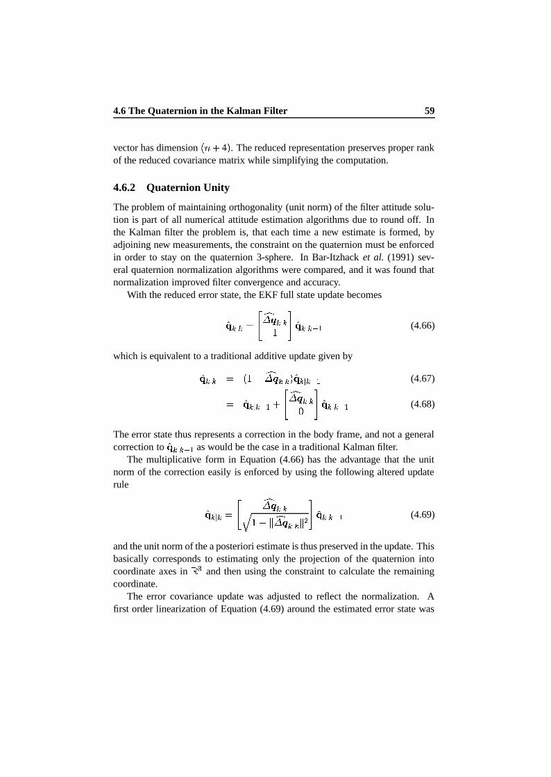
4.6 The Quaternion in the Kalman Filter 59
vector has dimension¯ �w£ � ³ . The reduced representation preserves proper rank
of the reduced covariance matrix while simplifying the computation.
4.6.2 Quaternion Unity
The problem of maintaining orthogonality (unit norm) of the filter attitude solu-tion is part of all numerical attitude estimation algorithms due to round off. Inthe Kalman filter the problem is, that each time a new estimate is formed, byadjoining new measurements, the constraint on the quaternion must be enforcedin order to stay on the quaternion 3-sphere. In Bar-Itzhack et al. (1991) sev-eral quaternion normalization algorithms were compared, and it was found thatnormalization improved filter convergence and accuracy.
With the reduced error state, the EKF full state update becomes�5 ¥ �Èê ëm«4 ¥ · í �5 ¥ Y » (4.66)
which is equivalent to a traditional additive update given by�5 ¥ � ¯ · £ ëm±4 ¥ ³��5 ¥ Y » (4.67)
� �5 ¥ Y » £åê ëm±4 ¥ � í �5 ¥ Y » (4.68)
The error state thus represents a correction in the body frame, and not a generalcorrection to
�5 ¥ Y » as would be the case in a traditional Kalman filter.The multiplicative form in Equation (4.66) has the advantage that the unit
norm of the correction easily is enforced by using the following altered updaterule �5 ¥ � ê ëm«4 ¥ î · � ¾ ëm±4 ¥ ¾ Â
í �5 ¥ Y » (4.69)
and the unit norm of the a posteriori estimate is thus preserved in the update. Thisbasically corresponds to estimating only the projection of the quaternion intocoordinate axes in
ÌoÎand then using the constraint to calculate the remaining
coordinate.The error covariance update was adjusted to reflect the normalization. A
first order linearization of Equation (4.69) around the estimated error state was
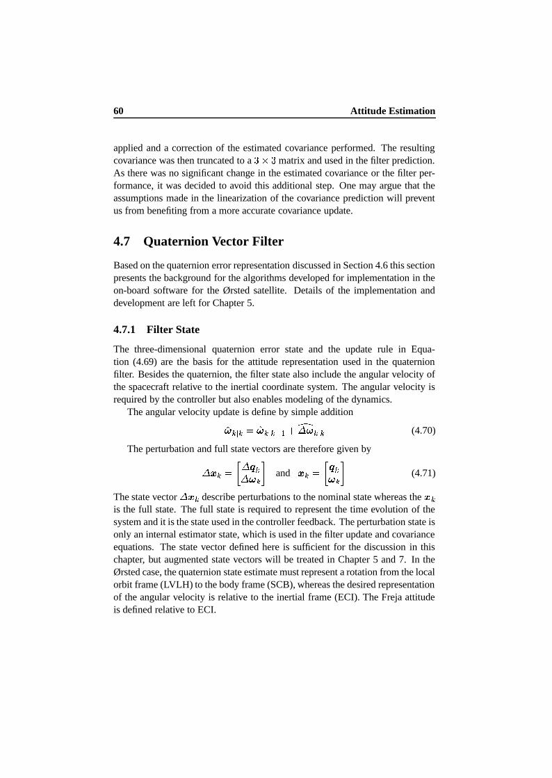
60 Attitude Estimation
applied and a correction of the estimated covariance performed. The resultingcovariance was then truncated to a
Ë � Ë matrix and used in the filter prediction.As there was no significant change in the estimated covariance or the filter per-formance, it was decided to avoid this additional step. One may argue that theassumptions made in the linearization of the covariance prediction will preventus from benefiting from a more accurate covariance update.
4.7 Quaternion Vector Filter
Based on the quaternion error representation discussed in Section 4.6 this sectionpresents the background for the algorithms developed for implementation in theon-board software for the Ørsted satellite. Details of the implementation anddevelopment are left for Chapter 5.
4.7.1 Filter State
The three-dimensional quaternion error state and the update rule in Equa-tion (4.69) are the basis for the attitude representation used in the quaternionfilter. Besides the quaternion, the filter state also include the angular velocity ofthe spacecraft relative to the inertial coordinate system. The angular velocity isrequired by the controller but also enables modeling of the dynamics.
The angular velocity update is define by simple addition�w ¥ � �w ¥ Y » £ Îm±w ¥ (4.70)
The perturbation and full state vectors are therefore given bym ¤ � @ m±4 mÓw B and ¤ � @ 4 w B (4.71)
The state vector m ¤ describe perturbations to the nominal state whereas the ¤ is the full state. The full state is required to represent the time evolution of thesystem and it is the state used in the controller feedback. The perturbation state isonly an internal estimator state, which is used in the filter update and covarianceequations. The state vector defined here is sufficient for the discussion in thischapter, but augmented state vectors will be treated in Chapter 5 and 7. In theØrsted case, the quaternion state estimate must represent a rotation from the localorbit frame (LVLH) to the body frame (SCB), whereas the desired representationof the angular velocity is relative to the inertial frame (ECI). The Freja attitudeis defined relative to ECI.
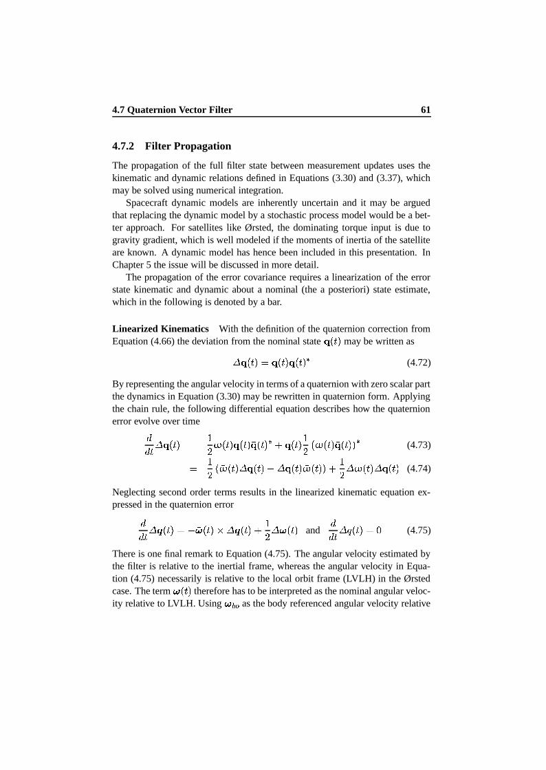
4.7 Quaternion Vector Filter 61
4.7.2 Filter Propagation
The propagation of the full filter state between measurement updates uses thekinematic and dynamic relations defined in Equations (3.30) and (3.37), whichmay be solved using numerical integration.
Spacecraft dynamic models are inherently uncertain and it may be arguedthat replacing the dynamic model by a stochastic process model would be a bet-ter approach. For satellites like Ørsted, the dominating torque input is due togravity gradient, which is well modeled if the moments of inertia of the satelliteare known. A dynamic model has hence been included in this presentation. InChapter 5 the issue will be discussed in more detail.
The propagation of the error covariance requires a linearization of the errorstate kinematic and dynamic about a nominal (the a posteriori) state estimate,which in the following is denoted by a bar.
Linearized Kinematics With the definition of the quaternion correction fromEquation (4.66) the deviation from the nominal state
Ö5 ¯lk�³may be written asm 5 ¯lkt³ � 5 ¯lkt³ Ö5 ¯lk�³ T (4.72)
By representing the angular velocity in terms of a quaternion with zero scalar partthe dynamics in Equation (3.30) may be rewritten in quaternion form. Applyingthe chain rule, the following differential equation describes how the quaternionerror evolve over time|| k m 5 ¯lkt³ � ·
�-ï ¯lk�³ 5 ¯lk�³ Ö5 ¯lkt³ T £ 5 ¯lkt³ ·� ¯ Öï ¯lk�³ Ö5 ¯lkt³t³ T (4.73)
� ·�¯ Öï ¯lk�³ m 5 ¯lk�³ �"m 5 ¯lk�³ Öï ¯lkt³t³ £ ·
� m ï ¯lk�³ m 5 ¯lk�³ (4.74)
Neglecting second order terms results in the linearized kinematic equation ex-pressed in the quaternion error|| k�m±4 ¯lk�³ ��� Öw ¯lk�³ ��m±4 ¯lkt³ £ ·
� mÓw ¯lkt³ and|| k�m±3 ¯lk�³ ��� (4.75)
There is one final remark to Equation (4.75). The angular velocity estimated bythe filter is relative to the inertial frame, whereas the angular velocity in Equa-tion (4.75) necessarily is relative to the local orbit frame (LVLH) in the Ørstedcase. The term
Öw ¯lkt³ therefore has to be interpreted as the nominal angular veloc-ity relative to LVLH. Using
Öw Ú � as the body referenced angular velocity relative
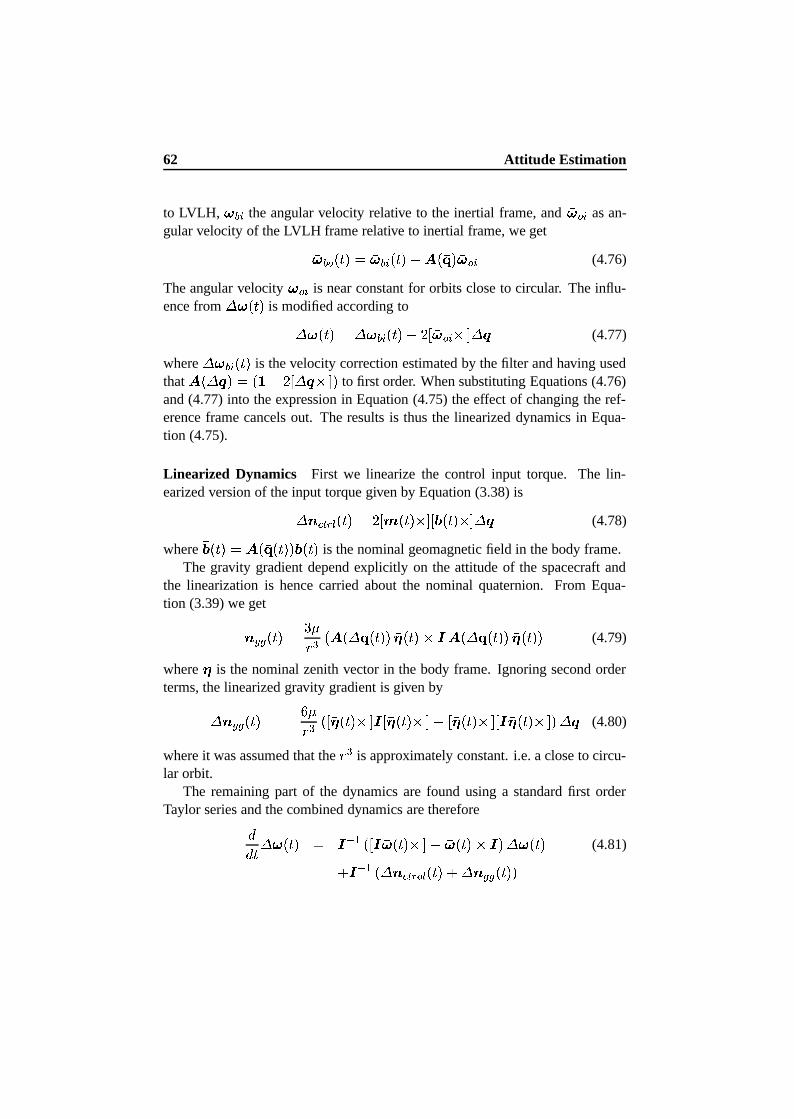
62 Attitude Estimation
to LVLH, w Ú ¡ the angular velocity relative to the inertial frame, andÖw � ¡ as an-
gular velocity of the LVLH frame relative to inertial frame, we getÖw Ú � ¯lk�³ � Öw Ú ¡ ¯lkt³ � ±«¯ Ö5 ³ Öw � ¡ (4.76)
The angular velocityÖw � ¡ is near constant for orbits close to circular. The influ-
ence from mÓw ¯lk�³ is modified according tomÓw ¯lkt³ ��mÓw Ú ¡ ¯lk�³ � ��ø Öw � ¡��ýúðm±4 (4.77)
where mÓw Ú ¡ ¯lkt³ is the velocity correction estimated by the filter and having usedthat
± ¯ m±4 ³ � ¯ ��� ��ø¶m±4"� ú ³ to first order. When substituting Equations (4.76)and (4.77) into the expression in Equation (4.75) the effect of changing the ref-erence frame cancels out. The results is thus the linearized dynamics in Equa-tion (4.75).
Linearized Dynamics First we linearize the control input torque. The lin-earized version of the input torque given by Equation (3.38) ism± U� ÏÑÐ8� ¯lk�³ � ��ø � ¯lk�³ � úø Ö¿ ¯lkt³ �{úðm±4 (4.78)
whereÖ¿ ¯lkt³ � ± ¯ Ö5 ¯lk�³t³ ¿ ¯lkt³ is the nominal geomagnetic field in the body frame.
The gravity gradient depend explicitly on the attitude of the spacecraft andthe linearization is hence carried about the nominal quaternion. From Equa-tion (3.39) we get ��� ¯lk�³ � Ë��� Î ¯Z± ¯ m 5 ¯lk�³t³ Ö�'¯lkt³ �P� ± ¯ m 5 ¯lk�³t³ Ö�À¯lkt³t³ (4.79)
whereÖ�
is the nominal zenith vector in the body frame. Ignoring second orderterms, the linearized gravity gradient is given bym± ñ��� ¯lk�³ � ò �� Î ¯ ø Ö�J¯lk�³ � úð�{ø Ö�"¯lkt³ � ú1�Åø Ö�J¯lk�³ � úø¶� Ö�"¯lkt³ � ú ³ m±4 (4.80)
where it was assumed that the � Î is approximately constant. i.e. a close to circu-lar orbit.
The remaining part of the dynamics are found using a standard first orderTaylor series and the combined dynamics are therefore|| k�mÓw ¯lk�³ � � Y » ¯ ø¶� Öw ¯lkt³ � ú1� Öw ¯lkt³ �ç� ³ mÓw ¯lk�³ (4.81)
£ó� Y » ¯ m« ñ� ÏÑÐ:�:� ¯lk�³ £<m« N�W� ¯lkt³t³
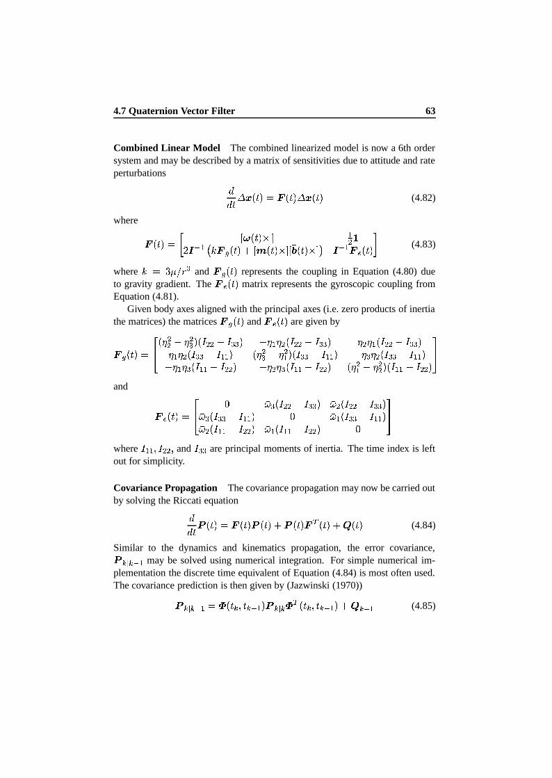
4.7 Quaternion Vector Filter 63
Combined Linear Model The combined linearized model is now a 6th ordersystem and may be described by a matrix of sensitivities due to attitude and rateperturbations || k m ¤ ¯lkt³ �Q¡ ¯lk�³ m ¤ ¯lk�³ (4.82)
where ¡ ¯lkt³ � @ �Qø Öw ¯lkt³ � ú »Â ���� Y » » Ä ¡«� ¯lkt³ £äø � ¯lk�³ � úø Ö¿ ¯lkt³ �{ú ½ � Y » ¡3¥ ¯lk�³ B (4.83)
whereÄ � Ë�� _ � Î and ¡«� ¯lk�³ represents the coupling in Equation (4.80) due
to gravity gradient. The ¡©¥ ¯lkt³ matrix represents the gyroscopic coupling fromEquation (4.81).
Given body axes aligned with the principal axes (i.e. zero products of inertiathe matrices) the matrices ¡V� ¯lkt³ and ¡3¥ ¯lk�³ are given by
¡ � ¯lkt³ � �� ¯ Öô  � Öô ÂÎ ³�¯·õ Ât � õ ÎtÎ ³ � Öô » Öô  ¯·õ Ât � õ ÎtÎ ³ Öô  Öô » ¯·õ Ât � õ ÎtÎ ³Öô » Öô  ¯·õ ÎtÎ � õ »t» ³ ¯ Öô ÂÎ � Öô » ³�¯·õ ÎtÎ � õ »t» ³ � Öô Î Öô  ¯·õ ÎtÎ � õ »t» ³� Öô » Öô Î ¯·õ »t»¶� õ Ât ³ � Öô  Öô Î ¯·õ »t»¶� õ Ât ³ ¯ Öô » � Öô  ³�¯·õ »t»°� õ Ât ³�
and ¡3¥ ¯lk�³ � �� � Öö Î ¯·õ Ât � õ ÎtÎ ³ Öö  ¯·õ Ât � õ ÎtÎ ³Öö Î ¯·õ ÎtÎ � õ »t» ³ � Öö » ¯·õ ÎtÎ � õ »t» ³Öö  ¯·õ »t»¶� õ Ât ³ Öö » ¯·õ »t»¶� õ Ât ³ ��
whereõ »t» Ö�õ ÂtÂ Ö and
õ ÎtÎ are principal moments of inertia. The time index is leftout for simplicity.
Covariance Propagation The covariance propagation may now be carried outby solving the Riccati equation|| k ¯ ¯lk�³ �Q¡ ¯lkt³ ¯ ¯lkt³ £6¯ ¯lkt³ ¡ýÕ ¯lkt³ £S¨ ¯lk�³ (4.84)
Similar to the dynamics and kinematics propagation, the error covariance,¯ ¥ Y » may be solved using numerical integration. For simple numerical im-plementation the discrete time equivalent of Equation (4.84) is most often used.The covariance prediction is then given by (Jazwinski (1970))¯ ¥ Y » ��Õ ¯lk Ö8k Y » ³ ¯ ¥ Õ Õ ¯lk Ö8k Y » ³ £<¨ Y » (4.85)
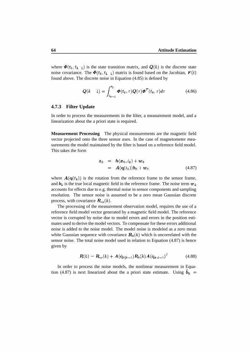
64 Attitude Estimation
where Õ ¯lk Ö8k Y » ³ is the state transition matrix, and ¨ ¯´Ä�³ is the discrete statenoise covariance. The Õ ¯lk Ö8k Y » ³ matrix is found based on the Jacobian, ¡ ¯lk�³found above. The discrete noise in Equation (4.85) is defined by¨ ¯´Ä � · ³ ��� Ï ÜÏ ÜW÷CÞ Õ ¯lk Ö ³ ¨ ¯ ³ Õ Õ ¯lk Ö ³ | (4.86)
4.7.3 Filter Update
In order to process the measurements in the filter, a measurement model, and alinearization about the a priori state is required.
Measurement Processing The physical measurements are the magnetic fieldvector projected onto the three sensor axes. In the case of magnetometer mea-surements the model maintained by the filter is based on a reference field model.This takes the form £ � � ¯ ¤ Ö8k ³ £�â � ± ¯
5¯lk ³t³ ¿ £�â (4.87)
where± ¯5¯lk ³t³ is the rotation from the reference frame to the sensor frame,
and ¿ is the true local magnetic field in the reference frame. The noise term â accounts for effects due to e.g. thermal noise in sensor components and samplingresolution. The sensor noise is assumed to be a zero mean Gaussian discreteprocess, with covariance ²°ø ¯´Ä�³ .
The processing of the measurement observation model, requires the use of areference field model vector generated by a magnetic field model. The referencevector is corrupted by noise due to model errors and errors in the position esti-mates used to derive the model vectors. To compensate for these errors additionalnoise is added to the noise model. The model noise is modeled as a zero meanwhite Gaussian sequence with covariance ² Ú ¯´Ä�³ which is uncorrelated with thesensor noise. The total noise model used in relation to Equation (4.87) is hencegiven by ² ¯´Ä�³ �Q² ø ¯´Ä�³ £ ± ¯Á�5 ¥ Y » ³ ² Ú ¯´Ä�³W±«¯Á�
5 ¥ Y » ³ Õ (4.88)
In order to process the noise models, the nonlinear measurement in Equa-tion (4.87) is next linearized about the a priori state estimate. Using
Ö¿ �
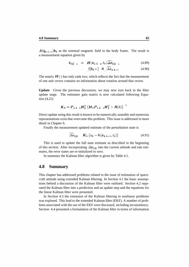
4.8 Summary 65
± ¯ �5 ¥ Y » ³ ¿ as the nominal magnetic field in the body frame. The result isa measurement equation given by�£ ¥ Y » � à ¯ �¤ ¥ Y » Ö8k ³ Î m ¤ ¥ Y » (4.89)
� ó ��ø Ö¿ � úåR ÷ Îm ¤ ¥ Y » (4.90)
The matrix à ¯ � ³ has only rank two, which reflects the fact that the measurementof one unit vector contains no information about rotation around that vector.
Update Given the previous discussion, we may now turn back to the filterupdate stage. The estimator gain matrix is now calculated following Equa-tion (4.22) º �Q¯ ¥ Y » Ã Õ »Åà ¯ ¥ Y » Ã Õ £<² ¯´Ä�³ ½ Y »Direct update using this result is known to be numerically unstable and numerousrepresentations exist that overcome this problem. This issue is addressed in moredetail in Chapter 6.
Finally the measurement updated estimate of the perturbation state isÎ m ¤ ¥ �Qº »ù£ �"� ¯��¤ ¥ Y » Ö8k ³ ½ (4.91)
This is used to update the full state estimate as described in the beginningof this section. After incorporating m ¤ ¥ into the current attitude and rate esti-mates, the error states are re-initialized to zero.
In summary the Kalman filter algorithm is given by Table 4.1.
4.8 Summary
This chapter has addressed problems related to the issue of estimation of space-craft attitude using extended Kalman filtering. In Section 4.1 the basic assump-tions behind a discussion of the Kalman filter were outlined. Section 4.2 sepa-rated the Kalman filter into a prediction and an update step and the equations forthe linear Kalman filter were presented.
In Section 4.3 the extension of the Kalman filtering to nonlinear problemswas explored. This lead to the extended Kalman filter (EKF). A number of prob-lems associated with the use of the EKF were discussed, including inconsistency.Section 4.4 presented a formulation of the Kalman filter in terms of information
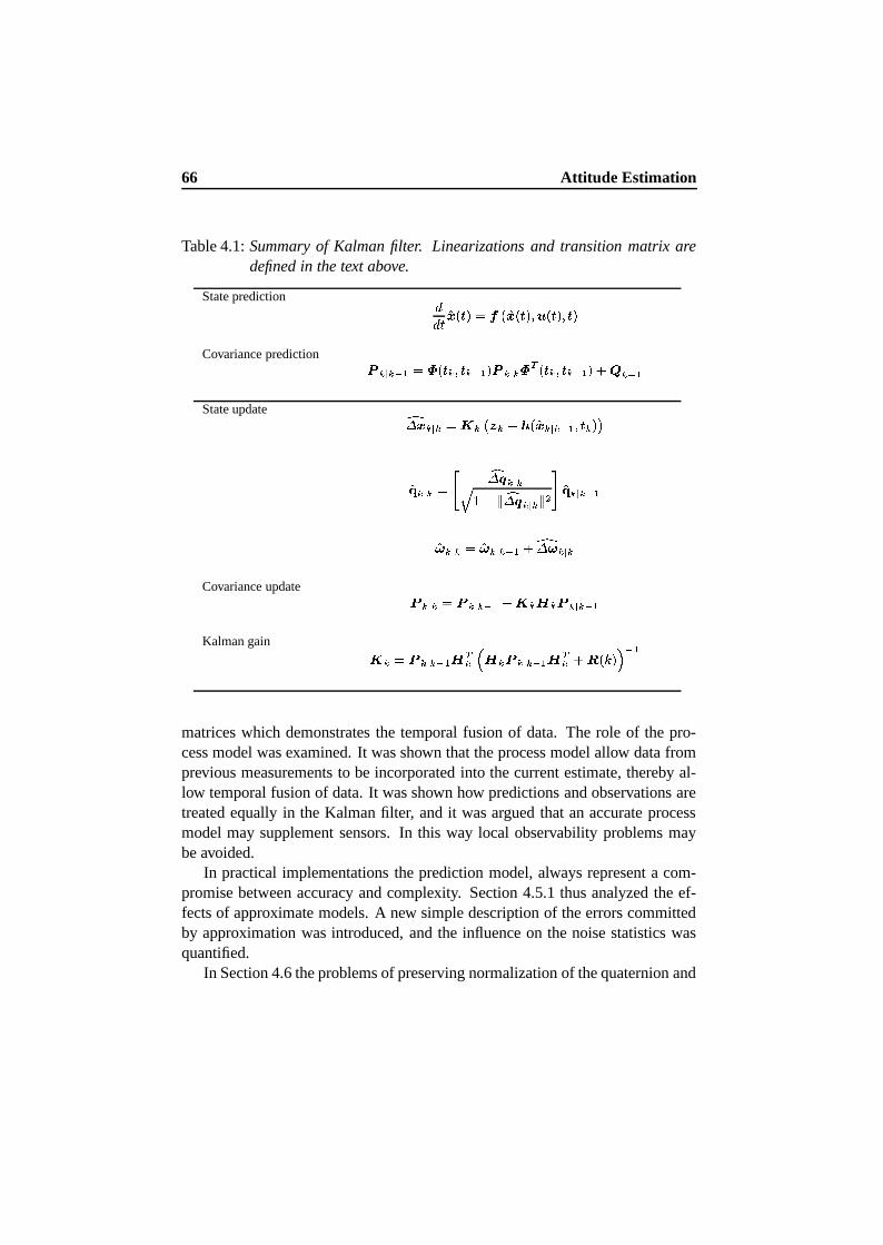
66 Attitude Estimation
Table 4.1: Summary of Kalman filter. Linearizations and transition matrix aredefined in the text above.
State prediction úú�û�üý+þ ûÅÿ ì�� þ üý�þ ûÅÿ é�� þ ûÅÿ é ûÅÿCovariance prediction � Ü�� ÜW÷&Þ ì�� þ û Ü é û Ü�÷&Þ ÿ � Ü�� Ü � í þ û Ü é û Ü�÷&Þ ÿ�� ÜW÷CÞState update � ý Ü�� Ü ì�� Ü����#Ü���� þ üý Ü�� ÜW÷CÞ é û Ü ÿ��
ü� Ü�� Ü ì � ���� Ü�� Ü� ��! ���� Ü"� Ü !$#&% ü� Ü�� ÜW÷CÞü' Ü�� Ü ì ü' Ü"� ÜW÷&Þ � ' Ü"� Ü
Covariance update � Ü�� Ü ì � Ü�� ÜW÷CÞ � � Ü�(�Ü � Ü�� Ü�÷&ÞKalman gain � Ü ì � Ü"� ÜW÷&Þ ( í Ü*) ( Ü � Ü�� ÜW÷CÞ ( í Ü �+ þ-, ÿ/. ÷&Þ
matrices which demonstrates the temporal fusion of data. The role of the pro-cess model was examined. It was shown that the process model allow data fromprevious measurements to be incorporated into the current estimate, thereby al-low temporal fusion of data. It was shown how predictions and observations aretreated equally in the Kalman filter, and it was argued that an accurate processmodel may supplement sensors. In this way local observability problems maybe avoided.
In practical implementations the prediction model, always represent a com-promise between accuracy and complexity. Section 4.5.1 thus analyzed the ef-fects of approximate models. A new simple description of the errors committedby approximation was introduced, and the influence on the noise statistics wasquantified.
In Section 4.6 the problems of preserving normalization of the quaternion and

4.8 Summary 67
covariance singularity were addressed. It was argued that a conventional EKFapproach is problematic due to a covariance singularity. The covariance singu-larity was demonstrated using the exponential series in the quaternion, whichwas truncated to first order. The first order approximation was finally used inSection 4.7, which presented a filter, which avoids the covariance singularity byusing a three dimensional first order approximation to the correction quaternioncalculated by the Kalman filter. The correction represents a rotation in the bodyframe.


Chapter 5
Ørsted Attitude Estimation
The original motivation for the work presented in this thesis was given by theattitude control system (ACS) for the Ørsted small satellite. The Ørsted mis-sion requires Earth-pointing three-axis control, which in turn demands that thespacecraft attitude determination system (ADS) provides accurate attitude of thevehicle. This chapter presents the design and evaluation of the ADS developedfor Ørsted. Results from the on-board implementation are discussed in Chap-ter 6. The main results in this chapter have been published in Bak (1996), Bak etal. (1996a), and Bak (1998a).
The chapter is divided into six sections plus conclusions. Section 5.1 presentsthe motivation for addressing the Ørsted problem and describes the underlyingproblems. Section 5.2 addresses the requirements to accuracy and fault toler-ance. The implications for estimator design are discussed. Section 5.3 takesthe first step in the development of the ADS. A simulation model is describedthat simulate the motion of the satellite as accurately as possible over a set oftest cases. Section 5.4 discusses the estimator design, and two different processmodels are presented. Section 5.5 presents the results for a set of scenarios rang-ing from a nominal pointing to a fault situation. Finally, Section 5.6 presents anerror budget which combines the effects of a number of systematic errors into anestimate of the predicted performance of the magnetometer based ADS.
5.1 Motivation and Related Work
Low-cost launch opportunities and technological advancements make smallsatellites interesting for doing space experiments within an affordable cost and
69
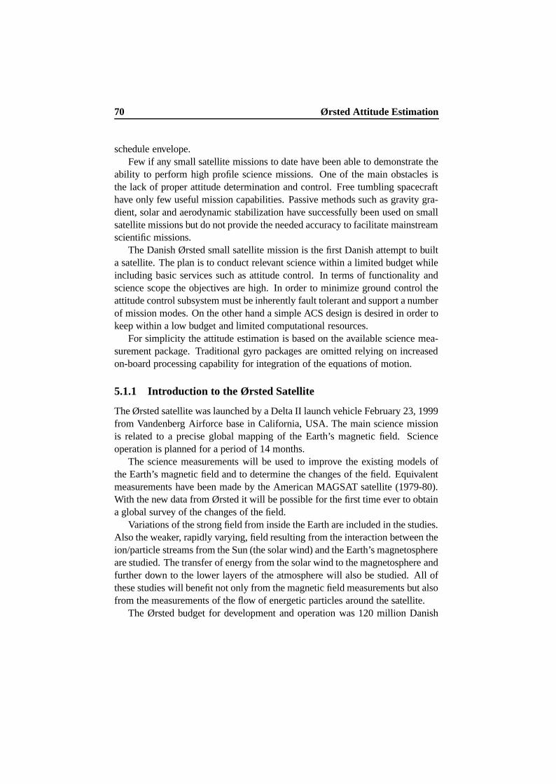
70 Ørsted Attitude Estimation
schedule envelope.Few if any small satellite missions to date have been able to demonstrate the
ability to perform high profile science missions. One of the main obstacles isthe lack of proper attitude determination and control. Free tumbling spacecrafthave only few useful mission capabilities. Passive methods such as gravity gra-dient, solar and aerodynamic stabilization have successfully been used on smallsatellite missions but do not provide the needed accuracy to facilitate mainstreamscientific missions.
The Danish Ørsted small satellite mission is the first Danish attempt to builta satellite. The plan is to conduct relevant science within a limited budget whileincluding basic services such as attitude control. In terms of functionality andscience scope the objectives are high. In order to minimize ground control theattitude control subsystem must be inherently fault tolerant and support a numberof mission modes. On the other hand a simple ACS design is desired in order tokeep within a low budget and limited computational resources.
For simplicity the attitude estimation is based on the available science mea-surement package. Traditional gyro packages are omitted relying on increasedon-board processing capability for integration of the equations of motion.
5.1.1 Introduction to the Ørsted Satellite
The Ørsted satellite was launched by a Delta II launch vehicle February 23, 1999from Vandenberg Airforce base in California, USA. The main science missionis related to a precise global mapping of the Earth’s magnetic field. Scienceoperation is planned for a period of 14 months.
The science measurements will be used to improve the existing models ofthe Earth’s magnetic field and to determine the changes of the field. Equivalentmeasurements have been made by the American MAGSAT satellite (1979-80).With the new data from Ørsted it will be possible for the first time ever to obtaina global survey of the changes of the field.
Variations of the strong field from inside the Earth are included in the studies.Also the weaker, rapidly varying, field resulting from the interaction between theion/particle streams from the Sun (the solar wind) and the Earth’s magnetosphereare studied. The transfer of energy from the solar wind to the magnetosphere andfurther down to the lower layers of the atmosphere will also be studied. All ofthese studies will benefit not only from the magnetic field measurements but alsofrom the measurements of the flow of energetic particles around the satellite.
The Ørsted budget for development and operation was 120 million Danish
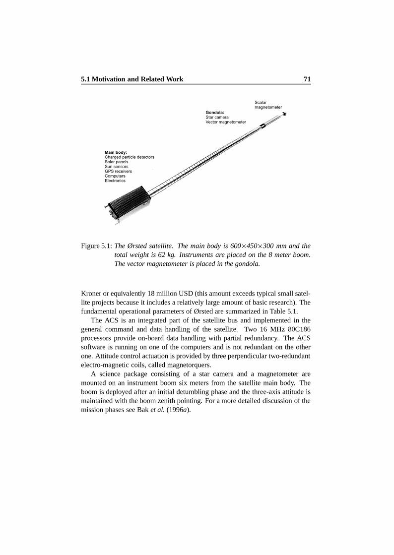
5.1 Motivation and Related Work 71
Figure 5.1: The Ørsted satellite. The main body is 600 � 450 � 300 mm and thetotal weight is 62 kg. Instruments are placed on the 8 meter boom.The vector magnetometer is placed in the gondola.
Kroner or equivalently 18 million USD (this amount exceeds typical small satel-lite projects because it includes a relatively large amount of basic research). Thefundamental operational parameters of Ørsted are summarized in Table 5.1.
The ACS is an integrated part of the satellite bus and implemented in thegeneral command and data handling of the satellite. Two 16 MHz 80C186processors provide on-board data handling with partial redundancy. The ACSsoftware is running on one of the computers and is not redundant on the otherone. Attitude control actuation is provided by three perpendicular two-redundantelectro-magnetic coils, called magnetorquers.
A science package consisting of a star camera and a magnetometer aremounted on an instrument boom six meters from the satellite main body. Theboom is deployed after an initial detumbling phase and the three-axis attitude ismaintained with the boom zenith pointing. For a more detailed discussion of themission phases see Bak et al. (1996a).
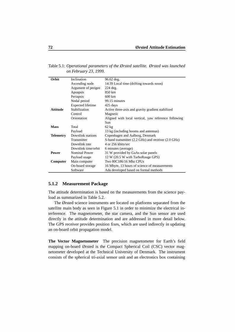
72 Ørsted Attitude Estimation
Table 5.1: Operational parameters of the Ørsted satellite. Ørsted was launchedon February 23, 1999.
Orbit Inclination 96.62 deg.Ascending node 14:39 Local time (drifting towards noon)Argument of perigee 224 deg.Apoapsis 850 kmPeriapsis 600 kmNodal period 99.15 minutesExpected lifetime 425 days
Attitude Stabilization Active three-axis and gravity gradient stabilizedControl MagneticOrientation Aligned with local vertical, yaw reference following
SunMass Total 62 kg
Payload 13 kg (including booms and antennas)Telemetry Downlink stations Copenhagen and Aalborg, Denmark
Transmitter S-band transmitter (2.2 GHz) and receiver (2.0 GHz)Downlink rate 4 or 256 kbits/secDownlink time/orbit 6 minutes (average)
Power Nominal Power 31 W provided by GaAs solar panelsPayload usage 12 W (20.5 W with TurboRouge GPS)
Computer Main computer Two 80C186/16 Mhz CPUsOn-board storage 16 Mbyte, 13 hours of science of measurementsSoftware Ada developed based on formal methods
5.1.2 Measurement Package
The attitude determination is based on the measurements from the science pay-load as summarized in Table 5.2.
The Ørsted science instruments are located on platforms separated from thesatellite main body as seen in Figure 5.1 in order to minimize the electrical in-terference. The magnetometer, the star camera, and the Sun sensor are useddirectly in the attitude determination and are addressed in more detail below.The GPS receiver provides position fixes, which are used indirectly in updatingan on-board orbit propagation model.
The Vector Magnetometer The precision magnetometer for Earth’s fieldmapping on-board Ørsted is the Compact Spherical Coil (CSC) vector mag-netometer developed at the Technical University of Denmark. The instrumentconsists of the spherical tri-axial sensor unit and an electronics box containing
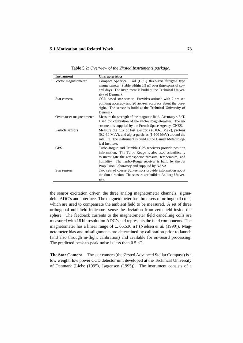
5.1 Motivation and Related Work 73
Table 5.2: Overview of the Ørsted Instruments package.
Instrument CharacteristicsVector magnetometer Compact Spherical Coil (CSC) three-axis fluxgate type
magnetometer. Stable within 0.5 nT over time spans of sev-eral days. The instrument is build at the Technical Univer-sity of Denmark
Star camera CCD based star sensor. Provides attitude with 2 arc-secpointing accuracy and 20 arc-sec accuracy about the bore-sight. The sensor is build at the Technical University ofDenmark.
Overhauser magnetometer Measure the strength of the magnetic field. Accuracy < 5nT.Used for calibration of the vector magnetometer. The in-strument is supplied by the French Space Agency, CNES.
Particle sensors Measure the flux of fast electrons (0.03-1 MeV), protons(0.2-30 MeV), and alpha-particles (1-100 MeV) around thesatellite. The instrument is build at the Danish Meteorolog-ical Institute.
GPS Turbo-Rogue and Trimble GPS receivers provide positioninformation. The Turbo-Rouge is also used scientificallyto investigate the atmospheric pressure, temperature, andhumidity. The Turbo-Rouge receiver is build by the JetPropulsion Laboratory and supplied by NASA
Sun sensors Two sets of coarse Sun-sensors provide information aboutthe Sun direction. The sensors are build at Aalborg Univer-sity.
the sensor excitation driver, the three analog magnetometer channels, sigma-delta ADC’s and interface. The magnetometer has three sets of orthogonal coils,which are used to compensate the ambient field to be measured. A set of threeorthogonal null field indicators sense the deviation from zero field inside thesphere. The feedback currents to the magnetometer field cancelling coils aremeasured with 18 bit resolution ADC’s and represents the field components. Themagnetometer has a linear range of 65.536 nT (Nielsen et al. (1990)). Mag-netometer bias and misalignments are determined by calibration prior to launch(and also through in-flight calibration) and available for on-board processing.The predicted peak-to-peak noise is less than 0.5 nT.
The Star Camera The star camera (the Ørsted Advanced Stellar Compass) is alow weight, low power CCD detector unit developed at the Technical Universityof Denmark (Liebe (1995), Jørgensen (1995)). The instrument consists of a
74 Ørsted Attitude Estimation
camera head unit with a commercial CCD detector, and a data processing unitequipped with an Intel 486 type processor. The processing unit contains twolarge star databases, which enable autonomous acquisition and tracking modeattitude determination. In tracking mode, the tracking is based on a sphericalleast squares fit between two consecutive images. The acquisition is based onpattern recognition of the stars in the field of view. Typically 65 stars in thefield of view are used for tracking. The camera field of view is 16 � 22 deg. andthe CCD has 752 � 582 pixels. The attitude is updated at approximately 0.8 Hzand give the attitude relative to the ECI inertial frame. The camera’s limit ofoperation is an angular rate of 10 deg./minute. Sun/Moon/Earth exposure mayalso cause temporary loss of attitude information. The instrument is mounted onthe boom next to the magnetometer in order to provide the highest accuracy inthe magnetometer attitude relative to the star camera. The predicted accuracy is2 arcsec (1 sigma) perpendicular to the boresight and 20 arcsec (1 sigma) aboutthe boresight (Eisenman et al. (1996))
The Wide-Angle Sun Sensor A low accuracy Sun sensor provides Sun posi-tion sensing over a near 4 0 steradian operating range. The instrument is buildat Aalborg University. The Sun sensors are comprised of eight independentGaAs cells, each operated in short circuit mode. The cells are mounted on themain structure in two three-axis assemblies and two single axis assemblies. Themounting of the sensors overcomes the field of view limitations otherwise im-posed by separation mechanism and antennas. Each of the eight Sun sensorheads has two-redundant cells and termistors for thermal compensation. Field ofview limitations and Earth albedo make the Sun sensors fairly nonlinear and theexpected accuracy of the calibrated sensors is about 4 deg. (1 sigma) about allthree axes.
5.1.3 The Attitude Control Subsystem
The Ørsted attitude control is implemented using magnetorquers as the sole con-trol devices. The attitude is estimated on-board using the available science sensorsuite. The nominal pointing requirements are derived from power optimizationas well as the operational cone and rate sensitivity of the star camera.
The control objectives of the ACS are related to
– Detumbling. Initially, after release from the launcher the satellite will ex-perience a tumbling motion. The objective of the ACS is to reduce the
5.1 Motivation and Related Work 75
kinetic energy. The satellite should be aligned with the local magneticfield, ready for boom deployment.
– Three-axis stabilization. After detumbling the boom is deployed and thesatellite should be three axes stabilized during the remainder of the mis-sion. The reference attitude is aligned with local vertical with boom zenithpointing. The angular deviation from vertical should be maintained withina 10 deg. (1 sigma) accuracy. The yaw reference is changing with lo-cal solar time and should be maintained within 20 deg. (1 sigma). Theangular velocity is required below 10 deg./minute at all time.
– Contingencies. A number of contingency situations are foreseen, includ-ing a boom down and a high spin rate mode. The ACS should handle thesecases autonomously and re-acquire the satellite.
– Autonomy A philosophy for the development of fault-tolerant control hasbeen adopted in the design of the ACS (Blanke (1995)). Autonomy isachieved through development of attitude determination and control al-gorithms that are reconfigurable in real time. This makes it possible toaccommodate changed mission phases, faults, and contingencies. An on-board supervisor (Bøgh et al. (1995)) monitors the spacecraft status andreconfigures ACS algorithms accordingly, to optimize the performanceof the system. All on-board autonomous transitions can be controlledthrough up-linked, time-tagged telecommands. Further operational flex-ibility is provided by allowing adjustments of flight software by upload asa last resort.
A number of ACS operational modes have been identified as reflected in theØrsted ACS architecture illustrated in Figure 5.2.
The initial rate detumbling relies entirely on the magnetometer measurementas a reference for damping the kinetic energy. After boom deployment the at-titude is stabilized in three axes and three axis attitude and rate information isdetermined by the ADS. The available input is data from the star camera, theSun sensor, and the magnetometer. An orbit model is dynamically updated fromground based on information from the GPS receiver. The attitude control algo-rithm determine a desired control torque that is used to compute the coil currentsbased on the measured geomagnetic field direction. A general introduction toattitude determination and control of the Ørsted satellite is provided in Bøgh etal. (1997). Details on the fault tolerant approach to ACS design and the atti-
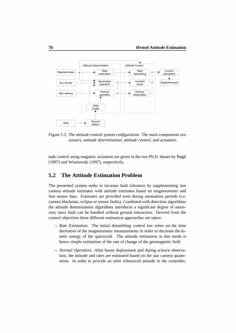
76 Ørsted Attitude Estimation
Figure 5.2: The attitude control system configuration. The main components aresensors, attitude determination, attitude control, and actuators.
tude control using magnetic actuation are given in the two Ph.D. theses by Bøgh(1997) and Wisniewski (1997), respectively.
5.2 The Attitude Estimation Problem
The presented system seeks to increase fault tolerance by supplementing starcamera attitude estimates with attitude estimates based on magnetometer andSun sensor data. Estimates are provided even during anomalous periods (i.e.camera blackouts, eclipse or sensor faults). Combined with detection algorithmsthe attitude determination algorithms introduces a significant degree of auton-omy since fault can be handled without ground interaction. Derived from thecontrol objectives three different estimation approaches are taken:
– Rate Estimation. The initial detumbling control law relies on the timederivative of the magnetometer measurements in order to decrease the ki-netic energy of the spacecraft. The attitude estimation in this mode ishence simple estimation of the rate of change of the geomagnetic field.
– Normal Operation. After boom deployment and during science observa-tion, the attitude and rates are estimated based on the star camera quater-nions. In order to provide an orbit referenced attitude to the controller,
5.2 The Attitude Estimation Problem 77
the cameras inertial attitude estimates are transformed with orbit positioninformation into local attitude and rate estimates. The pointing require-ments translate into requirements to the on-board attitude knowledge. Thepitch/roll requirement is 2 deg. (1 sigma). The yaw requirement is 4 deg.(1 sigma). The error in the rate estimates should be below �ai h � · � Y >rad/sec (1 sigma). With the star camera accuracy these modest require-ments are not a problem.
– Secondary Operation. For contingency situations where the star cameraattitude is not available, a secondary operation mode is available. Situa-tions may include high angular rates, a boom down situation and camerablackouts due to bright objects in the field of view. The secondary opera-tion is based on measurements from the Sun sensor and the magnetometer.The measurements are filtered by an EKF that computes attitude and rateestimates from the measured magnetic field and Sun vector together withmodel vectors of the geomagnetic field and the Sun direction.
After boom deployment the star camera estimates the attitude with uniqueaccuracy provided the operational constraints of the camera are satisfied. Prior toboom deployment and in situations with faults or temporary blackout, alternativesources of information are needed to maintain adequate attitude information forcontrol.
Rather than using sensor fusion techniques where all sensors are combined inone algorithm, the problem was separated into two parallel problems. The nor-mal operation problem based on the star camera, and the secondary operationproblem where the attitude estimates are based on the Sun sensor and magne-tometer.
This decision has several consequences:
– Reduced complexity. In the nominal situation where the star camera is pro-viding the attitude, the on-board computation is simplified significantly.The complex Kalman filter algorithm is only a backup.
– Parallel development. The two different algorithms may be developed inparallel. As design and tests of the nominal situation were scheduled priorto the different backup solutions, a simple normal operation mode wasdesirable.
– Two independent on-board estimates. Two estimates are available on-board for fault detection and integrity monitoring.
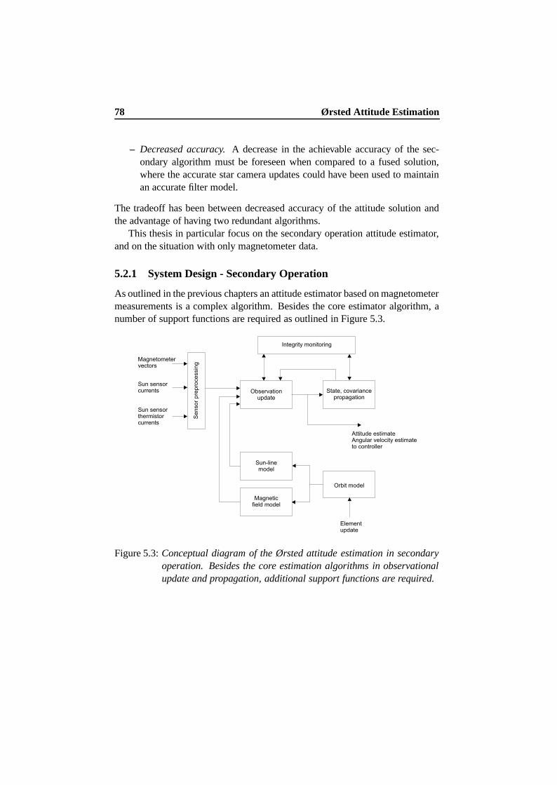
78 Ørsted Attitude Estimation
– Decreased accuracy. A decrease in the achievable accuracy of the sec-ondary algorithm must be foreseen when compared to a fused solution,where the accurate star camera updates could have been used to maintainan accurate filter model.
The tradeoff has been between decreased accuracy of the attitude solution andthe advantage of having two redundant algorithms.
This thesis in particular focus on the secondary operation attitude estimator,and on the situation with only magnetometer data.
5.2.1 System Design - Secondary Operation
As outlined in the previous chapters an attitude estimator based on magnetometermeasurements is a complex algorithm. Besides the core estimator algorithm, anumber of support functions are required as outlined in Figure 5.3.
Figure 5.3: Conceptual diagram of the Ørsted attitude estimation in secondaryoperation. Besides the core estimation algorithms in observationalupdate and propagation, additional support functions are required.
5.2 The Attitude Estimation Problem 79
Integrity Monitoring Faulty measurements and possible non-convergence ofthe filter must be detected autonomously on-board in order to achieve as high alevel of autonomy as possible with simple means.
The variance of the Kalman filter innovation sequence is assumed zero meanand the variance is given by the elements of ø¶Ã ¯ Ã Õ £�² ¯´Ä�³ ú . This is ex-ploited for the practical purposes of sensor failure detection and outlier detectionof the measurement data. During operation of the filter, the innovation sequenceis monitored and compared to this description. If the description is violated con-sistently, the filter process is declared faulty.
Innovation monitoring is also used for outlier checking of the measurementsbefore they are processed by the filter. If a measurement residual is greater thanthe 3 1 value computed by the filter, it is not processed. However, if this happensfrequently, the cause may be either a sensor failure or a filter divergence problem.In the latter case, it is critical not to reject large residuals, since they are the onlymeans of correcting the divergence. In the Ørsted control system, an approachhas, however, been taken based on the simple 3 1 in order to simplify the detector.The test levels may be modified from ground as flight experience is gained. Amore elegant approach would be based on an online statistical test as outlined inSection 7.4.1.1 but this was rejected as part of a general software reduction.
Orbit Model Ørsted is equipped with on-board GPS receivers, which, in thenominal situation, determines a state vector, consisting of position and velocity.The raw GPS measurements are osculating elements and hence not suited forsimple propagation, which is based on mean elements. Test have shown thatusing raw GPS measurements in the orbit propagation resulted in errors of 12 kmafter just 16 hours (Bak (1995)).
An orbit model concept is therefore adopted based on the assumption thatthe GPS is not directly available for on-board ACS processing. The orbit prop-agation on-board is based on simple Kepler propagation with mean elementsuploaded from ground every seven days. The model incorporates the primary
® Âgravitational perturbational effect on the orbit plane, which is represented by aconstant drift rate for the ascending node and the apsidal line as a function oftime.
The upload parameters are estimated on ground using a least square fit overseven days of propagated orbit positions from the high accuracy ground prop-agation model. The model provides an estimated accuracy of 15 km (1 sigma)over a seven day period (See Appendix B).
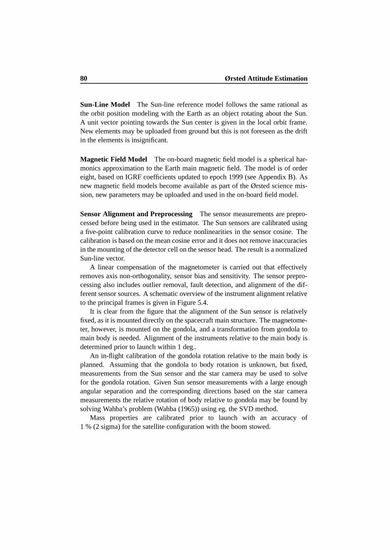
80 Ørsted Attitude Estimation
Sun-Line Model The Sun-line reference model follows the same rational asthe orbit position modeling with the Earth as an object rotating about the Sun.A unit vector pointing towards the Sun center is given in the local orbit frame.New elements may be uploaded from ground but this is not foreseen as the driftin the elements is insignificant.
Magnetic Field Model The on-board magnetic field model is a spherical har-monics approximation to the Earth main magnetic field. The model is of ordereight, based on IGRF coefficients updated to epoch 1999 (see Appendix B). Asnew magnetic field models become available as part of the Ørsted science mis-sion, new parameters may be uploaded and used in the on-board field model.
Sensor Alignment and Preprocessing The sensor measurements are prepro-cessed before being used in the estimator. The Sun sensors are calibrated usinga five-point calibration curve to reduce nonlinearities in the sensor cosine. Thecalibration is based on the mean cosine error and it does not remove inaccuraciesin the mounting of the detector cell on the sensor head. The result is a normalizedSun-line vector.
A linear compensation of the magnetometer is carried out that effectivelyremoves axis non-orthogonality, sensor bias and sensitivity. The sensor prepro-cessing also includes outlier removal, fault detection, and alignment of the dif-ferent sensor sources. A schematic overview of the instrument alignment relativeto the principal frames is given in Figure 5.4.
It is clear from the figure that the alignment of the Sun sensor is relativelyfixed, as it is mounted directly on the spacecraft main structure. The magnetome-ter, however, is mounted on the gondola, and a transformation from gondola tomain body is needed. Alignment of the instruments relative to the main body isdetermined prior to launch within 1 deg..
An in-flight calibration of the gondola rotation relative to the main body isplanned. Assuming that the gondola to body rotation is unknown, but fixed,measurements from the Sun sensor and the star camera may be used to solvefor the gondola rotation. Given Sun sensor measurements with a large enoughangular separation and the corresponding directions based on the star camerameasurements the relative rotation of body relative to gondola may be found bysolving Wahba’s problem (Wahba (1965)) using eg. the SVD method.
Mass properties are calibrated prior to launch with an accuracy of1 % (2 sigma) for the satellite configuration with the boom stowed.
5.3 Simulation Models 81
Figure 5.4: Ørsted alignment tree.
The next section begins the task of developing and analyzing the ADCthrough the identification of a simulation model.
5.3 Simulation Models
An accurate simulation (or truth) model is significant for the development of anADS. The simulation model replaces the real physical system with a simula-tion, which realistically models the behavior of the satellite system. It yields theappropriate observations, which would be acquired by a given sensor. Withinthis methodology, a candidate system is designed, tuned and its performance as-sessed with respect to the simulation model. Since the data is simulated the truestate of the spacecraft is known and the filter statistics can be easily calculated.With an accurate simulation model, the results obtained from it should apply tothe actual spacecraft with a high degree of confidence.
Results from computer simulations integrating models of the sensors, thespacecraft, and its on-orbit environment are presented to demonstrate projectedperformance capability. Figure 5.5 gives an overview of the simulation modeldeveloped for Ørsted.
The simulation model is a powerful tool for system design only if it modelsthe behavior of the true system with a high degree of accuracy. Sections 5.3.1 and5.3.2 describe the properties of respectively the dynamics and sensor models. Adescription of the environmental models used in the simulation model are given
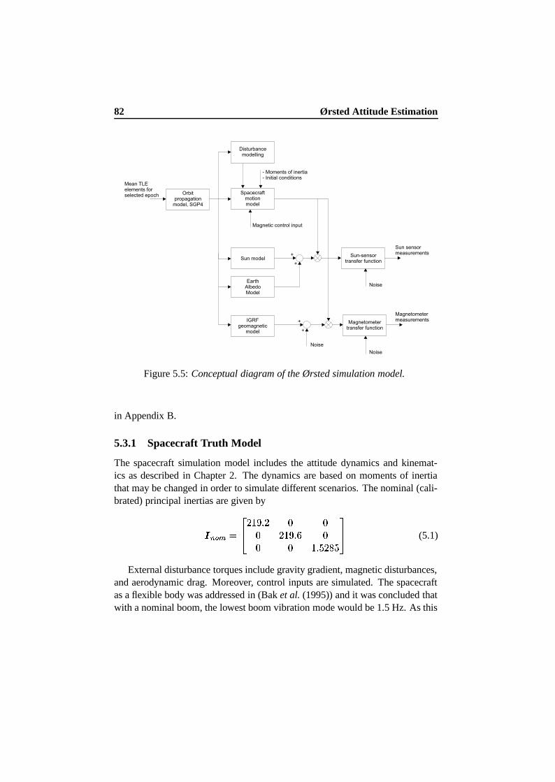
82 Ørsted Attitude Estimation
Figure 5.5: Conceptual diagram of the Ørsted simulation model.
in Appendix B.
5.3.1 Spacecraft Truth Model
The spacecraft simulation model includes the attitude dynamics and kinemat-ics as described in Chapter 2. The dynamics are based on moments of inertiathat may be changed in order to simulate different scenarios. The nominal (cali-brated) principal inertias are given by
� ¸ � ø � �� � ·32 i � � �� � ·32 i ò �� � · i54�� h 4�
(5.1)
External disturbance torques include gravity gradient, magnetic disturbances,and aerodynamic drag. Moreover, control inputs are simulated. The spacecraftas a flexible body was addressed in (Bak et al. (1995)) and it was concluded thatwith a nominal boom, the lowest boom vibration mode would be 1.5 Hz. As this
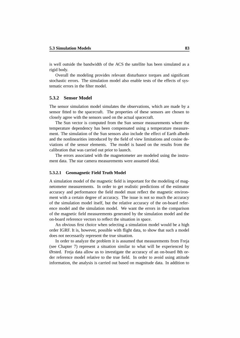
5.3 Simulation Models 83
is well outside the bandwidth of the ACS the satellite has been simulated as arigid body.
Overall the modeling provides relevant disturbance torques and significantstochastic errors. The simulation model also enable tests of the effects of sys-tematic errors in the filter model.
5.3.2 Sensor Model
The sensor simulation model simulates the observations, which are made by asensor fitted to the spacecraft. The properties of these sensors are chosen toclosely agree with the sensors used on the actual spacecraft.
The Sun vector is computed from the Sun sensor measurements where thetemperature dependency has been compensated using a temperature measure-ment. The simulation of the Sun sensors also include the effect of Earth albedoand the nonlinearities introduced by the field of view limitations and cosine de-viations of the sensor elements. The model is based on the results from thecalibration that was carried out prior to launch.
The errors associated with the magnetometer are modeled using the instru-ment data. The star camera measurements were assumed ideal.
5.3.2.1 Geomagnetic Field Truth Model
A simulation model of the magnetic field is important for the modeling of mag-netometer measurements. In order to get realistic predictions of the estimatoraccuracy and performance the field model must reflect the magnetic environ-ment with a certain degree of accuracy. The issue is not so much the accuracyof the simulation model itself, but the relative accuracy of the on-board refer-ence model and the simulation model. We want the errors in the comparisonof the magnetic field measurements generated by the simulation model and theon-board reference vectors to reflect the situation in space.
An obvious first choice when selecting a simulation model would be a highorder IGRF. It is, however, possible with flight data, to show that such a modeldoes not necessarily represent the true situation.
In order to analyze the problem it is assumed that measurements from Freja(see Chapter 7) represent a situation similar to what will be experienced byØrsted. Freja data allow us to investigate the accuracy of an on-board 8th or-der reference model relative to the true field. In order to avoid using attitudeinformation, the analysis is carried out based on magnitude data. In addition to
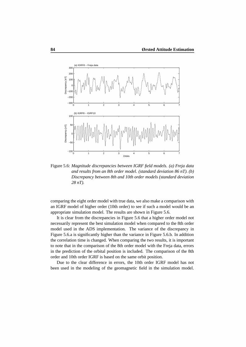
84 Ørsted Attitude Estimation
0 1 2 3 4 5 6 7−300
−200
−100
0
100
200
300D
iscr
epan
cy [n
T]
0 1 2 3 4 5 6 7−100
−50
0
50
100
Dis
crep
ancy
[nT
]
Orbits
(a) IGRF8 − Freja data
(b) IGRF8 − IGRF10
Figure 5.6: Magnitude discrepancies between IGRF field models. (a) Freja dataand results from an 8th order model. (standard deviation 86 nT). (b)Discrepancy between 8th and 10th order models (standard deviation28 nT).
comparing the eight order model with true data, we also make a comparison withan IGRF model of higher order (10th order) to see if such a model would be anappropriate simulation model. The results are shown in Figure 5.6.
It is clear from the discrepancies in Figure 5.6 that a higher order model notnecessarily represent the best simulation model when compared to the 8th ordermodel used in the ADS implementation. The variance of the discrepancy inFigure 5.6.a is significantly higher than the variance in Figure 5.6.b. In additionthe correlation time is changed. When comparing the two results, it is importantto note that in the comparison of the 8th order model with the Freja data, errorsin the prediction of the orbital position is included. The comparison of the 8thorder and 10th order IGRF is based on the same orbit position.
Due to the clear difference in errors, the 10th order IGRF model has notbeen used in the modeling of the geomagnetic field in the simulation model.
5.3 Simulation Models 85
The simulation model used in the Ørsted estimator design, is based on an 8thorder model, but it is augmented with a noise representation of the discrepancyin Figure 5.6.a.
To generate an error model for the results in Figure 5.6.a the errors wereanalyzed by looking at the auto-correlation and corresponding power spectraldensity (PSD). The PSD plot is shown in Figure 5.7.
10−4
10−3
10−2
10−1
100
10−2
100
102
104
106
Frequency [Hz]
Pow
er s
pect
ral d
ensi
ty [n
T2 s]
Figure 5.7: Power spectral density plot for the magnitude error in Figure 5.6.a.
The power spectral density curve in Figure 5.7 is approximated by a second-order Markov sequence, which provides a model of the oscillatory random phe-nomena in Figure 5.6.a. Data are fitted using subspace identification (Overscheeand Moor (1996)). The result is a colored noise model of the form¤ » ¯´Ä £ · ³ � ¡» ¤ » ¯´Ä�³ £ØÙª»�6 ¯´Ä�³ (5.2)7 » ¯´Ä�³ � ÃÓ» ¤ » ¯´Ä�³ (5.3)
where ¡´» ÆÓÌ Â �  , Ù¦» ÆÓÌ Â � » Ö Ã » ÆÓÌ » �  , and 6 ¯´Ä�³ is a white Gaussiannoise sequence with
©±ª 6Ô¡86ÃÄ Õ ¬ � ü�¡[¨ . The output of the noise model, 7 » ¯´Ä�³ ,represents the magnitude disturbance, which must be added to the output fromthe field model in order to reconstruct the (magnitude) error characteristics ofFreja data.
It is assumed that the magnitude errors are representative for the errors alsoperpendicular to the field vectors. Two additional noise sequences, 7  ¯´Ä�³*Ö 7 Î ¯´Ä�³similar to Equation (5.2) are constructed and added perpendicular to the IGRF
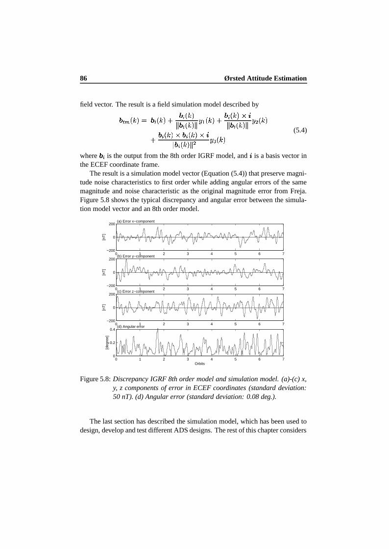
86 Ørsted Attitude Estimation
field vector. The result is a field simulation model described by
¿ Ï ø ¯´Ä�³ �ö¿�¡ ¯´Ä�³ £ ¿�¡ ¯´Ä�³¾*¿ ¡ ¯´Ä�³ ¾ 7 » ¯´Ä�³ £ ¿�¡ ¯´Ä�³ �ç7
¾*¿ ¡ ¯´Ä�³ ¾ 7  ¯´Ä�³£ ¿�¡ ¯´Ä�³ �ª¿�¡ ¯´Ä�³ �ç7
¾*¿�¡ ¯´Ä�³ ¾  7 Î ¯´Ä�³ (5.4)
where ¿�¡ is the output from the 8th order IGRF model, and 7 is a basis vector inthe ECEF coordinate frame.
The result is a simulation model vector (Equation (5.4)) that preserve magni-tude noise characteristics to first order while adding angular errors of the samemagnitude and noise characteristic as the original magnitude error from Freja.Figure 5.8 shows the typical discrepancy and angular error between the simula-tion model vector and an 8th order model.
0 1 2 3 4 5 6 7−200
0
200
[nT
]
0 1 2 3 4 5 6 7−200
0
200
[nT
]
0 1 2 3 4 5 6 7−200
0
200
[nT
]
0 1 2 3 4 5 6 70
0.2
0.4
Orbits
[deg
ree]
(a) Error x−component
(b) Error y−component
(c) Error z−component
(d) Angular error
Figure 5.8: Discrepancy IGRF 8th order model and simulation model. (a)-(c) x,y, z components of error in ECEF coordinates (standard deviation:50 nT). (d) Angular error (standard deviation: 0.08 deg.).
The last section has described the simulation model, which has been used todesign, develop and test different ADS designs. The rest of this chapter considers
5.4 Estimator Design 87
the development of the ADS. The core estimation algorithms have already beendiscussed and it remains to discuss the details in the implementation, and todemonstrate and test the capabilities of the attitude estimation
5.4 Estimator Design
In this section the design of the estimator is established and its performanceis evaluated with respect to the simulation model. The development process isiterative and requires a large amount of simulation and evaluation of models.The presentation here, highlights some of the more important steps taken in thedesign
– Process model. Two different process models are evaluated. The processmodel and the corresponding noise model are treated. The tradeoff be-tween model complexity and performance is discussed.
– Sensor model. The white Gaussian assumption on the sensor noise is dis-cussed on the basis of an analysis of magnetic field models.
– Evaluation. The estimator designs are evaluated and the performance pre-dicted.
The estimator design will focus on the ADS based on magnetometer measure-ments only. Inclusion of Sun vector measurements was discussed in Bak (1994).
5.4.1 Process Models
The model selection plays an integral role in the design of a model basedestimator. The main problem is the difficulty of obtaining an accurate spacecraftdynamic model. The dynamic model presented in Chapter 3 is sensitive touncertainty in the spacecraft moments of inertia and the external torque input.This problem has been recognized in previous work. Psiaki et al. (1990)suggested modeling the external torques as a random-walk process while Gaiet al. (1985) used a first-order Markov process to model rate disturbances. In arecent paper (Oshman and Markley (1999)) the dynamic model was completelyomitted, but the spacecraft angular acceleration was modeled as a first-orderMarkov process.
The choice of process model for Ørsted was based on the following observa-tions
88 Ørsted Attitude Estimation
– The satellite is gravity gradient stabilized. The influence from gravity gra-dient may be small at the reference (zenith pointing), but when the satellitemoves away from local vertical, the influence from the restoring gravitytorques becomes significant. For large angular deviations from local ver-tical, the gravity torque is larger than the possible control torques.
– The main uncertainty associated with explicit dynamic modeling is due tothe uncertainty in the moments of inertia. The inertias are calibrated priorto launch to an accuracy of 1 % (2 sigma). Only the satellite configurationwith boom stowed is calibrated, and the boom deployed inertias are thusmore uncertain.
– An in-flight calibration of the moments of inertia based on star cameraattitude in combination with a control torque excitation is planned. Thedynamic model may be adjusted accordingly in-flight.
– As Ørsted is a geomagnetic research satellite, the residual magnetic mo-ment in the structure is tightly controlled, and the dominating externaltorques, after the gravity gradient, is that caused by aerodynamic drag.The uncertainty involved in modeling of the drag is significant due to thecomplex structure of the boom and the uncertainty of atmospheric density.
Following the observations above, the process model is designed with explicitdynamic models, which include gravity gradient. The problem remaining is tomodel external torques and inertia uncertainty. Selecting a filter model whichyields optimal results is not a trivial process, as a more complex filter model withmore states might not lead to better performance because of the bias/variancetradeoff discussed in Chapter 4. This motivates an approach where two modelsare examined:
– P1 model. This model includes the gravity gradient explicitly, but all ex-ternal disturbances and inertia uncertainties are modeled as a white noiseprocess. A purely Gaussian model of the disturbance is selected, morebecause of its mathematical convenience, than its ability to accurately de-scribe the estimation errors.
– P2 model. In addition to explicit modeling of the gravity gradient torque,this process model includes a stochastic modeling of the external torquesas a Markov process. Based on an investigation of the typical disturbancetorques environment, the disturbance is modeled as an exponentially cor-related process driven by zero-mean Gaussian noise.
5.4 Estimator Design 89
The first of the two models is clearly an advantage from an implementation pointof view, as it reduces the complexity of the filter. The penalty is that the processnoise must be increased to account for unmodeled disturbances.
The P1 model The P1 process model follows the equations of motion as de-scribed by the Equations (3.30), (3.37) and (3.39) and the perturbation state vec-tor is given by m ¤ ) »o�A@ m±4mÓwdB (5.5)
No explicit modeling of the aerodynamic drag disturbance is included due to thecomplexity of such a model. This may lead to reduced accuracy, but the pricemay be acceptable as long as the results are within specifications, and the filteris consistent. The selection of process noise associated with P1 is discussed inSection 5.4.2.
The P2 model This model augment the state vector with extra states to allowthe filter to estimate the influence of the aerodynamic drag torque input. Theinvestigation of the drag torque environment is based on a series of simulationswith the simulation model. A typical example of the aerodynamic drag torqueis shown in Figure 5.9. For comparison the rate influence from gravity gradientis approximately (Wertz (1978))
Î:9Ð æ ¯·õ »t»o� õ ÎtÎ ³ � Û Ë i h � · � Y > Nm at a �Ê� · �deg. offset from local vertical.
As the satellite body coordinate system in Figure 5.9 is approximately alignedwith LVLH frame, the disturbance, � ¾ (pitch torque) dominates, which is notsurprising as this represents the torque resulting from aerodynamic drag on theboom structure. Due to the relative low inertia about the ; axis, also the torque�=< is significant. The disturbance in 7 is small as this axis is nominally alignedwith the velocity vector. The periodic component of the signals is correlated withthe orbital period and caused by the increase in atmospheric density at perigee.
The aerodynamic drag disturbance is dependent on the attitude of the satel-lite. Given a 90 deg. rotation in yaw, the dominating disturbance would be in7 rather than > . To allow for this attitude dependence to be expressed in themodel, the aerodynamic drag is modeled in the orbit frame. The aerodynamicmodel output is rotated to the body frame using the a posteriori estimate of theattitude prior to inclusion in the dynamic model. Allowing the attitude to dis-tribute the drag along different axis does not include the changes in the drag
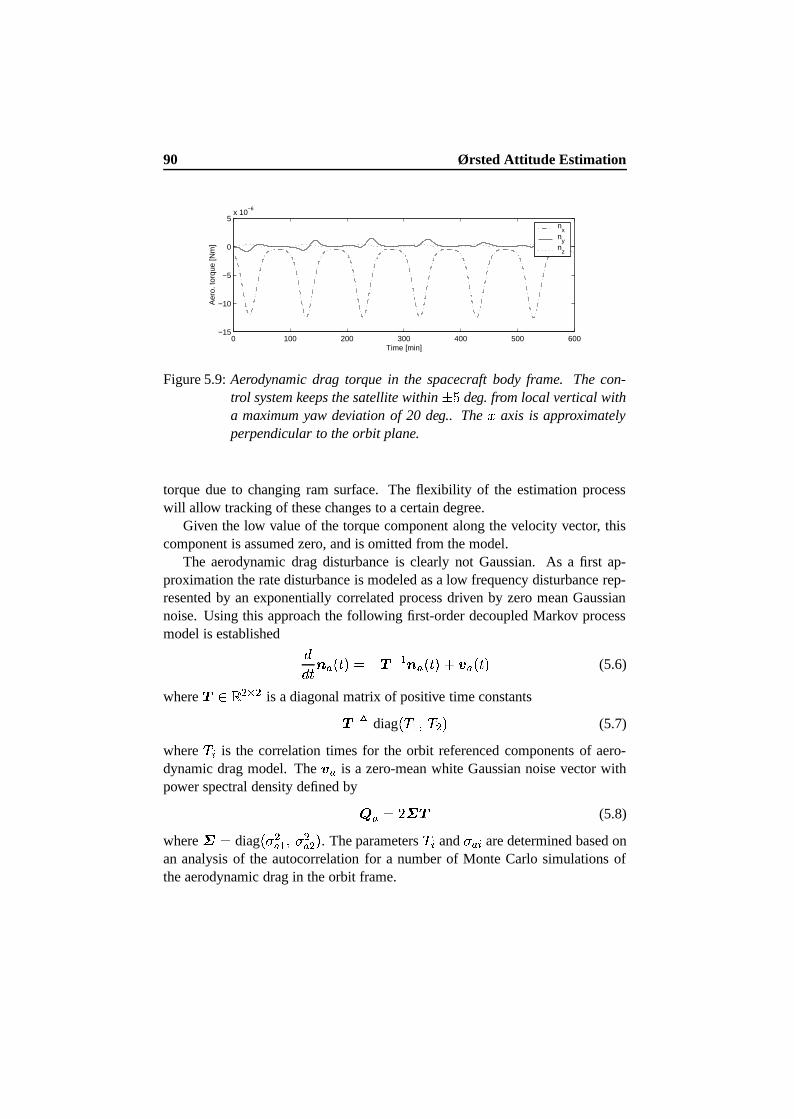
90 Ørsted Attitude Estimation
0 100 200 300 400 500 600−15
−10
−5
0
5x 10
−6
Time [min]
Aer
o. to
rque
[Nm
]
nx
ny
nz
Figure 5.9: Aerodynamic drag torque in the spacecraft body frame. The con-trol system keeps the satellite within ?4 deg. from local vertical witha maximum yaw deviation of 20 deg.. The > axis is approximatelyperpendicular to the orbit plane.
torque due to changing ram surface. The flexibility of the estimation processwill allow tracking of these changes to a certain degree.
Given the low value of the torque component along the velocity vector, thiscomponent is assumed zero, and is omitted from the model.
The aerodynamic drag disturbance is clearly not Gaussian. As a first ap-proximation the rate disturbance is modeled as a low frequency disturbance rep-resented by an exponentially correlated process driven by zero mean Gaussiannoise. Using this approach the following first-order decoupled Markov processmodel is established || k � ¯lk�³ ���A@ Y » � ¯lkt³ £�á � ¯lk�³ (5.6)
where @ Æ¢Ì Â �  is a diagonal matrix of positive time constants@ µdiag
¯ �V» Ö � Â ³ (5.7)
where ��¡ is the correlation times for the orbit referenced components of aero-dynamic drag model. The á � is a zero-mean white Gaussian noise vector withpower spectral density defined by ¨ � �ä�CB�@ (5.8)
where B � diag¯ 1 Â� » Ö 1 Â�  ³ . The parameters �b¡ and 1 � ¡ are determined based on
an analysis of the autocorrelation for a number of Monte Carlo simulations ofthe aerodynamic drag in the orbit frame.
5.4 Estimator Design 91
It is clear that for large angular deviations from local vertical, the aerody-namic torques will change significantly, and it is hence necessary to restrict theanalysis to a set of scenarios, which are close (<20 deg.) to local vertical. Theseall represent realistic situations for the satellite in normal operation.
Different yaw references would also influence the drag model, and in suchcases new parameters might be up-linked. This representation is of cause some-what restricted and it will slowly degrade and problems may arise when largeangular motion is considered.
The two states described by Equation (5.6) are augmented to the state vectorand the estimates of � are added in the dynamic equation. The augmented statevector for the P2 model is given bym ¤ )  � �� m±4mÓw �
� (5.9)
which has dimension eight. Adding two extra states adds to the complexity of thefiltering process, and the tradeoff remains between accuracy and complexity. Amore complex second order Markov model has been investigated, but was foundnot to give satisfactory results.
This section has described two different process models for the system. TheP1 model assumes a simple six dimensional state space representation, whichdoes not explicitly include aerodynamic drag. The P2 model include estimationof the aerodynamic drag influence by augmenting the state vector with two extrastates.
5.4.2 Process Noise Models
Process noises take account of all the discrepancies between the nominal processmodel and the actual behaviour of the spacecraft. They can be classified as twodifferent types
– Disturbances which act as input and include errors in the coil currents andaerodynamic drag.
– Noises that act on satellite parameters (in this case moments of inertia) asa result of the actual value of the parameters being unknown.
– Stabilizing noises. These are used to compensate for other unmodelederror sources like linearization. Often these noises have no clear physicalbasis but are required to ensure successful filter operation.
92 Ørsted Attitude Estimation
The process noise models are for the two process models are described in thefollowing.
Input Noise The coil currents in the torquer coils are measured directly and themeasurements are assumed corrupted by additive, zero mean uncorrelated noisesources, which have a Gaussian distribution. The corruption is due to samplingand resistor tolerances. Misalignment of the coils is difficult to quantify, and isassumed negligible as the coils are an integral parts of the satellite structure.
The influence of aerodynamic drag in the P1 model is compensated for byincreasing the input noise variance. In this way the simplicity obtained by not in-cluding explicit aerodynamic modeling is traded against increased process noise.The noise on the three angular velocity components is assumed uncorrelated andthe spectral density given by¨�D � diag
¯ 1 ÂD » Ö 1 ÂD Â Ö 1 ÂD Î ³ (5.10)
As the P2 process model include the aerodynamic drag effects explicitly, therequired injection of input noise is lower as for the P1 model. Under the assump-tion that the aerodynamic modeling is perfect, the P2 input noise set to zero.
Parameter Noise The second type of process noise affects the spacecraft pa-rameters. The only parameters in the process model, which are uncertain are themoments of inertia in the dynamics, and the correlation time in the aerodynamicmodeling. The modeling error due to errors in the moments of inertia has aneffect on the satellite dynamics propagation. The influence is analyzed in thefollowing.
The moments of inertia are calibrated prior to launch to an accuracy of 1%(2 sigma) in all three axes. The inertias for the satellite configuration with boomdeployed is then extrapolated based on inertia information for all structural ele-ments. It is assumed that this will result in an increase in the uncertainty to 2%(2 sigma).
Assuming that the angular velocity is represented in the principal frame, andleaving out control input, the dynamics (Equation (3.37)) may be rewritten inscalar form as Æö »o�FE�» ö  ö Î � Ä E�» ô  ô Î £®� D »Æö  �FE  ö Î ö » � Ä E  ô Î ô »V£®� D ÂÆö Î �FE Î ö » ö  � Ä E Î ô » ô  £®� D Î
5.4 Estimator Design 93
where � D ¡ is process noise contaminating the process,Ä � Ë�� _ � Î is the gravity
constant and E » � õ Ât � õ ÎtÎõ »t» E  � õ ÎtÎ � õ »t»õ Ât E Î � õ »t»¶� õ ÂtÂõ ÎtÎ (5.11)
whereõ ¡ ¡ are the principal moments of inertia.
As a result of the uncertainty in the calibration of the moments of inertia, theEÔ¡ parameters used in the filter process model will deviate from the true parame-ters. Systematic errors like this cannot directly be modeled using Gaussian whitenoise processes. One possibility is to estimate them as part of an augmented statevector (see the Freja case in Chapter 7). In the Ørsted case, the systematic ef-fects due to the E ¡ parameter errors are attempted compensated by increasing thevariance of the process noise. Combined with a possible in-flight calibration ofthe inertias, this reduces the complexity of the model.
The translation from a systematic error in the inertia parameters into covari-ance is not really well defined. The 2% variance on the inertia matrix diagonalelements is transformed into the corresponding variance the for the 1 ¡ parame-ters, and a square matrix describing the squared uncertainties in the parametersis defined by ¨HG � ÄI diag
¯ mJE Â » Ö mJE ÂÂ Ö mKE ÂÎ ³ (5.12)
whereÄ I
is a tuning parameter. Once the variance has been established on theinertias, the noise acting on the angular rate state is then obtained by a transfor-mation into the state space using the noise input matricesÙ¥ � diag
¯ ö Â ö Î Ö ö Î ö » Ö ö » ö Â ³ (5.13)Ù � � diag¯ � ô Â ô Î Ö � ô Î ô » Ö � ô » ô Â ³ (5.14)
The spectral density of the rate noise due to uncertainty in the inertias is thengiven by ¨ D ¡ � Ù¥W¨ I Ù©Õ¥ £ØÙ �c¨ I Ù©Õ � (5.15)
The noise description in Equation (5.15) is dependent on the actual state of thesystem. Intuitively the error committed in the state propagation must be smallfor small rates while larger for faster motion of the satellite. This intuition isreflected in the covariance in Equation (5.15).
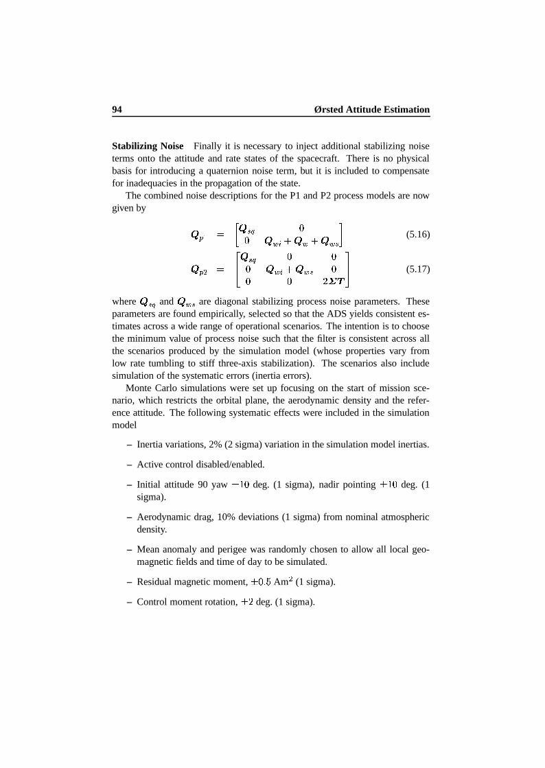
94 Ørsted Attitude Estimation
Stabilizing Noise Finally it is necessary to inject additional stabilizing noiseterms onto the attitude and rate states of the spacecraft. There is no physicalbasis for introducing a quaternion noise term, but it is included to compensatefor inadequacies in the propagation of the state.
The combined noise descriptions for the P1 and P2 process models are nowgiven by ¨ ) » � @ ¨ I ã �� ¨ D ¡ £<¨ D £6¨ D I B (5.16)
¨ )  ��� ¨ I ã � �� ¨ D ¡ £6¨ D I �� � �CB�@
� (5.17)
where ¨ I ã and ¨ D I are diagonal stabilizing process noise parameters. Theseparameters are found empirically, selected so that the ADS yields consistent es-timates across a wide range of operational scenarios. The intention is to choosethe minimum value of process noise such that the filter is consistent across allthe scenarios produced by the simulation model (whose properties vary fromlow rate tumbling to stiff three-axis stabilization). The scenarios also includesimulation of the systematic errors (inertia errors).
Monte Carlo simulations were set up focusing on the start of mission sce-nario, which restricts the orbital plane, the aerodynamic density and the refer-ence attitude. The following systematic effects were included in the simulationmodel
– Inertia variations, 2% (2 sigma) variation in the simulation model inertias.
– Active control disabled/enabled.
– Initial attitude 90 yaw · � deg. (1 sigma), nadir pointing · � deg. (1sigma).
– Aerodynamic drag, 10% deviations (1 sigma) from nominal atmosphericdensity.
– Mean anomaly and perigee was randomly chosen to allow all local geo-magnetic fields and time of day to be simulated.
– Residual magnetic moment, �ai54 Am  (1 sigma).
– Control moment rotation, l� deg. (1 sigma).
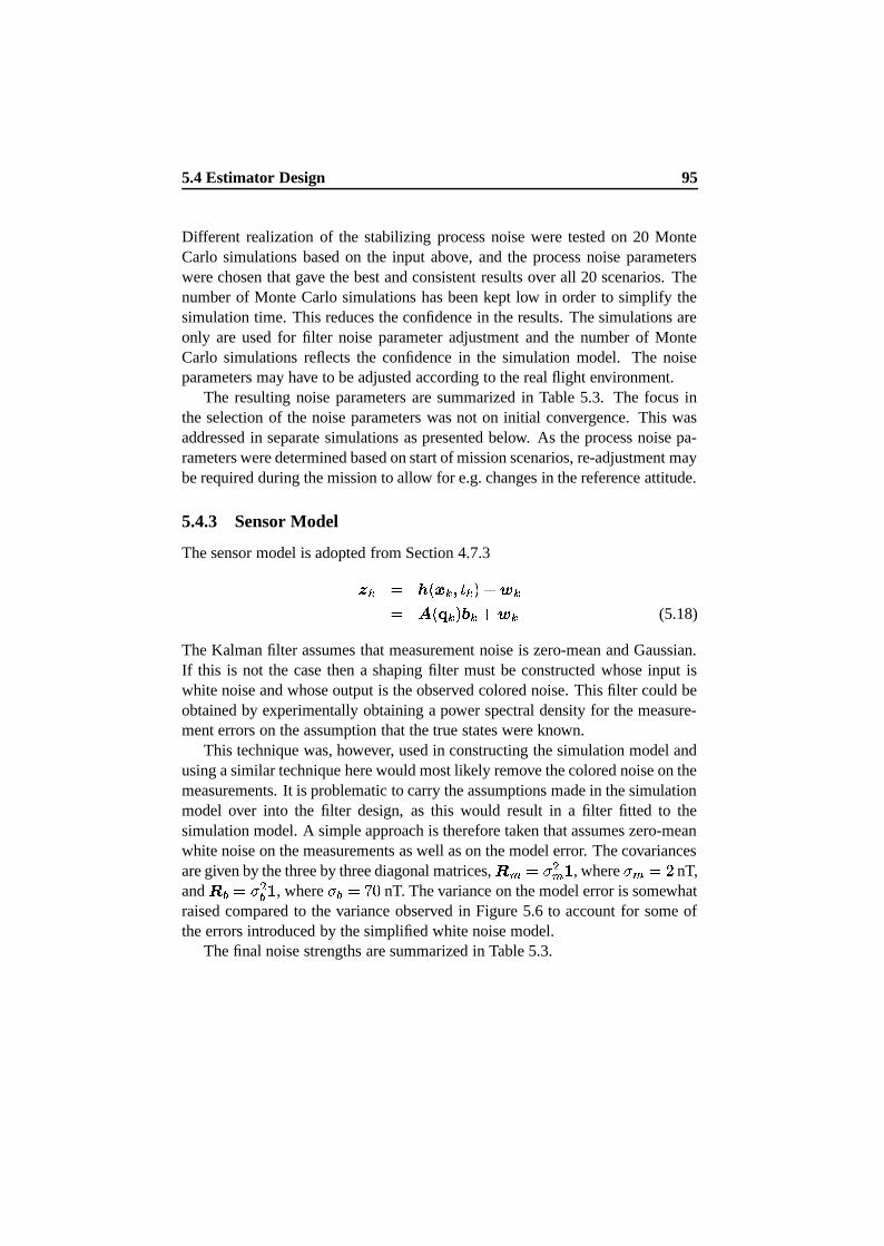
5.4 Estimator Design 95
Different realization of the stabilizing process noise were tested on 20 MonteCarlo simulations based on the input above, and the process noise parameterswere chosen that gave the best and consistent results over all 20 scenarios. Thenumber of Monte Carlo simulations has been kept low in order to simplify thesimulation time. This reduces the confidence in the results. The simulations areonly are used for filter noise parameter adjustment and the number of MonteCarlo simulations reflects the confidence in the simulation model. The noiseparameters may have to be adjusted according to the real flight environment.
The resulting noise parameters are summarized in Table 5.3. The focus inthe selection of the noise parameters was not on initial convergence. This wasaddressed in separate simulations as presented below. As the process noise pa-rameters were determined based on start of mission scenarios, re-adjustment maybe required during the mission to allow for e.g. changes in the reference attitude.
5.4.3 Sensor Model
The sensor model is adopted from Section 4.7.3£ � � ¯ ¤ Ö8k ³ £�â � ± ¯5 ³ ¿ £¤â (5.18)
The Kalman filter assumes that measurement noise is zero-mean and Gaussian.If this is not the case then a shaping filter must be constructed whose input iswhite noise and whose output is the observed colored noise. This filter could beobtained by experimentally obtaining a power spectral density for the measure-ment errors on the assumption that the true states were known.
This technique was, however, used in constructing the simulation model andusing a similar technique here would most likely remove the colored noise on themeasurements. It is problematic to carry the assumptions made in the simulationmodel over into the filter design, as this would result in a filter fitted to thesimulation model. A simple approach is therefore taken that assumes zero-meanwhite noise on the measurements as well as on the model error. The covariancesare given by the three by three diagonal matrices, ² ø �L1 Âø � , where 1 ø � � nT,and ² Ú �F1 ÂÚ � , where 1 Ú �NM�� nT. The variance on the model error is somewhatraised compared to the variance observed in Figure 5.6 to account for some ofthe errors introduced by the simplified white noise model.
The final noise strengths are summarized in Table 5.3.
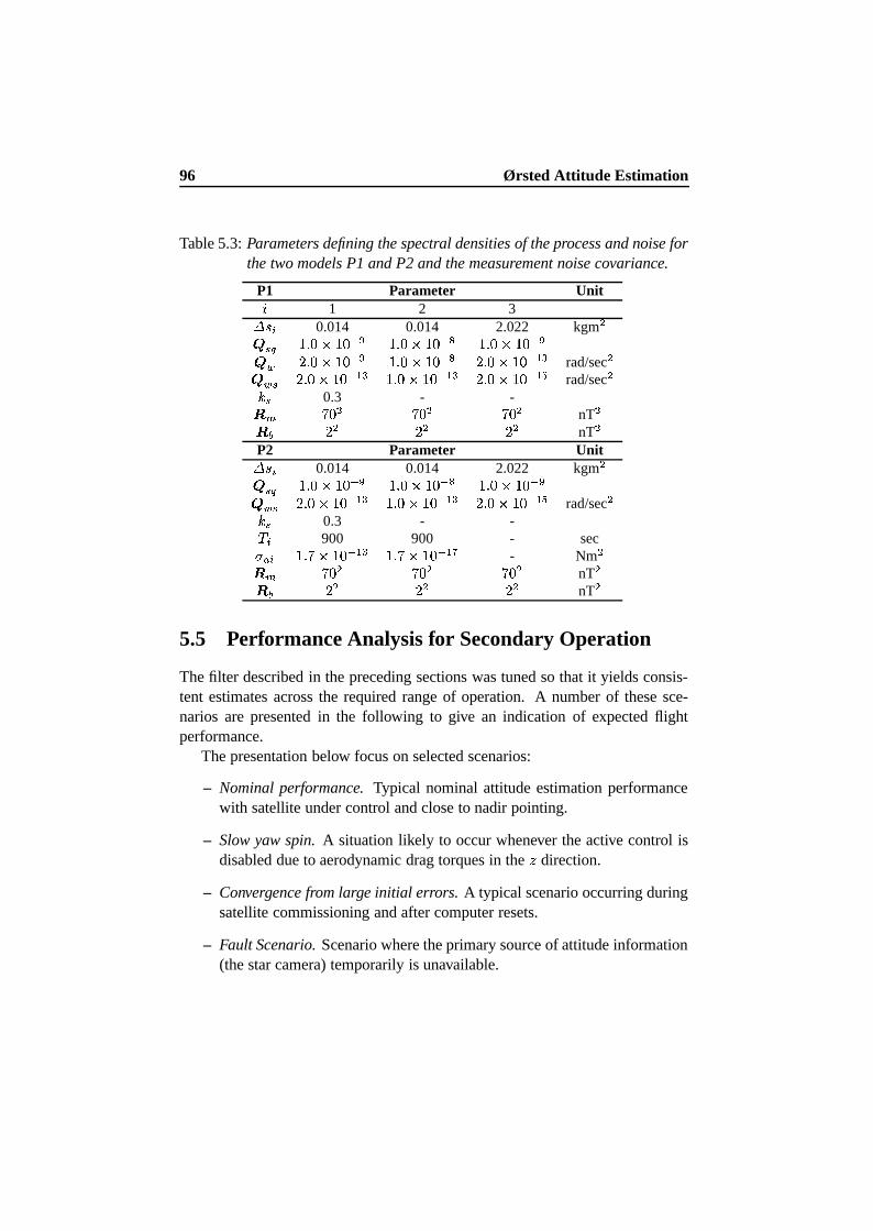
96 Ørsted Attitude Estimation
Table 5.3: Parameters defining the spectral densities of the process and noise forthe two models P1 and P2 and the measurement noise covariance.
P1 Parameter UnitO1 2 3j ~ a 0.014 0.014 2.022 kgm _�� � &QP )P�(&*) �SR &TP )ï�©&�) �VU &QP )P�(&*) �SR_�� W P )P�(&*) �SR &TP )ï�©&�) �VU W P )ï�(&*) ���Z rad/sec _���� W P )ï�(&*) ���Z &TP )P�©&�) ���B W P )ï�(&*) ���8X rad/sec 4 � 0.3 - -0 n Y ) Y ) Y ) nT 0 � W W W nT
P2 Parameter Unitj ~ a 0.014 0.014 2.022 kgm _�� � &QP )P�(&*) �SR &TP )ï�©&�) �VU &QP )P�(&*) �SR_���� W P )ï�(&*) ���Z &TP )P�©&�) ���B W P )ï�(&*) ���8X rad/sec 4 � 0.3 - -� a 900 900 - secZ z a &QP Y �(&*) ���Z &TP Y �©&�) ���&[ - Nm 0 n Y ) Y ) Y ) nT 0 � W W W nT
5.5 Performance Analysis for Secondary Operation
The filter described in the preceding sections was tuned so that it yields consis-tent estimates across the required range of operation. A number of these sce-narios are presented in the following to give an indication of expected flightperformance.
The presentation below focus on selected scenarios:
– Nominal performance. Typical nominal attitude estimation performancewith satellite under control and close to nadir pointing.
– Slow yaw spin. A situation likely to occur whenever the active control isdisabled due to aerodynamic drag torques in the ; direction.
– Convergence from large initial errors. A typical scenario occurring duringsatellite commissioning and after computer resets.
– Fault Scenario. Scenario where the primary source of attitude information(the star camera) temporarily is unavailable.

5.5 Performance Analysis for Secondary Operation 97
The net effects of all modeled error sources is investigated by comparingthe simulation model quantities to the corresponding estimates generated by thefilter. The difference between the estimated value and its corresponding simula-tion model value is the actual estimation error for this quantity. As an additionalcheck, the errors generated in this type of analysis are compared to the standarddeviations predicted by the filter.
5.5.1 Nominal Attitude
The nominal attitude scenario focus on a situation where the spacecraft is underactive control. The attitude is initially offset by 10 deg. in pitch. The pitch angleis gradually damped by the control system as shown in Figure 5.10.
The yaw reference in this scenario is 90 deg. (start of mission reference atti-tude), which results in the 7 axis being approximately perpendicular to the orbitplane. The angular velocities are nominally zero in > and ; , while the nominalrate about the 7 -axis is approximately · � · � Y Î rad/sec.
P1 Model Typical nominal attitude estimation performance for the P1 modelis shown in Figure 5.11.
The error in attitude estimates, represented by pitch, yaw and roll angles aswell as errors in the angular velocity are shown. Standard deviation (2 sigma)bounds are calculated by taking the square root of the diagonals of the estimatedcovariances and multiplying the result by two. Providing the filter is consistentlytuned, the state errors should lie within these bounds at least 2 4]\ of the time.
As a result of the tuning philosophy that focus on achieving consistent resultsfor all scenarios, the results in Figure 5.11 do not represent the best achievableresults for that specific scenario, but represents a compromise over a number ofcases.
The state errors in Figure 5.11 are approximately zero mean and bounded bythe two standard deviation curves and the covariance estimate is thus compatiblewith the actual errors. The accuracy of the yaw estimate is lower than the esti-mates of pitch and roll. This is due to the relative lower ; -axis inertia, and theaerodynamic drag disturbance.
The periodic nature of the standard deviation profiles in Figure 5.11 are dueto the periodic changes in the magnetic field vector. As an example look at theyaw errors. As the field is close to parallel to the ; -axis (over pole and southpole) the system is not observable in yaw, resulting in an increase in the yawcovariance estimate, see Figure 5.12.
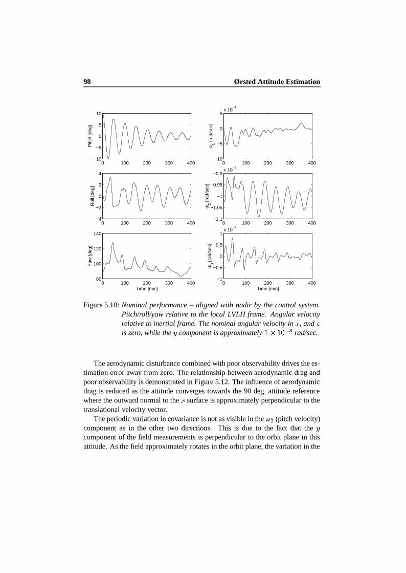
98 Ørsted Attitude Estimation
0 100 200 300 400−10
−5
0
5
10
Pitc
h [d
eg]
0 100 200 300 400−4
−2
0
2
4
Rol
l [de
g]
0 100 200 300 40080
100
120
140
Yaw
[deg
]
Time [min]
0 100 200 300 400−10
−5
0
5x 10
−4
ω1 [r
ad/s
ec]
0 100 200 300 400−1.1
−1.05
−1
−0.95
−0.9x 10
−3
ω2 [r
ad/s
ec]
0 100 200 300 400−1
−0.5
0
0.5
1x 10
−3
ω3 [r
ad/s
ec]
Time [min]
Figure 5.10: Nominal performance – aligned with nadir by the control system.Pitch/roll/yaw relative to the local LVLH frame. Angular velocityrelative to inertial frame. The nominal angular velocity in > , and ;is zero, while the 7 component is approximately · � · � Y Î rad/sec.
The aerodynamic disturbance combined with poor observability drives the es-timation error away from zero. The relationship between aerodynamic drag andpoor observability is demonstrated in Figure 5.12. The influence of aerodynamicdrag is reduced as the attitude converges towards the 90 deg. attitude referencewhere the outward normal to the > surface is approximately perpendicular to thetranslational velocity vector.
The periodic variation in covariance is not as visible in the ö Â (pitch velocity)component as in the other two directions. This is due to the fact that the 7component of the field measurements is perpendicular to the orbit plane in thisattitude. As the field approximately rotates in the orbit plane, the variation in the
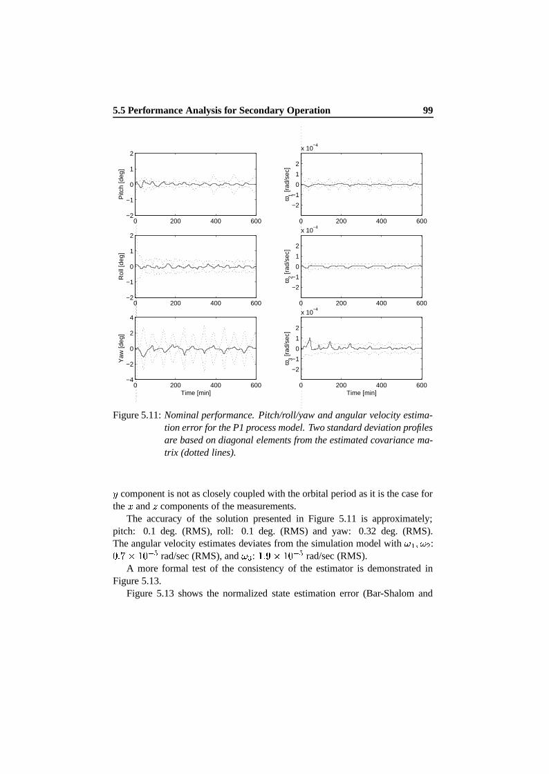
5.5 Performance Analysis for Secondary Operation 99
0 200 400 600−2
−1
0
1
2
Pitc
h [d
eg]
0 200 400 600−2
−1
0
1
2
Rol
l [de
g]
0 200 400 600−4
−2
0
2
4
Yaw
[deg
]
Time [min]
0 200 400 600
−2
−1
0
1
2
x 10−4
ω1 [r
ad/s
ec]
0 200 400 600
−2
−1
0
1
2
x 10−4
ω2 [r
ad/s
ec]
0 200 400 600
−2
−1
0
1
2
x 10−4
ω3 [r
ad/s
ec]
Time [min]
Figure 5.11: Nominal performance. Pitch/roll/yaw and angular velocity estima-tion error for the P1 process model. Two standard deviation profilesare based on diagonal elements from the estimated covariance ma-trix (dotted lines).
7 component is not as closely coupled with the orbital period as it is the case forthe > and ; components of the measurements.
The accuracy of the solution presented in Figure 5.11 is approximately;pitch: 0.1 deg. (RMS), roll: 0.1 deg. (RMS) and yaw: 0.32 deg. (RMS).The angular velocity estimates deviates from the simulation model with ö » Ö ö Â :�ai^M � · � Y`_ rad/sec (RMS), and ö Î : · i 2 � · � Y`_ rad/sec (RMS).
A more formal test of the consistency of the estimator is demonstrated inFigure 5.13.
Figure 5.13 shows the normalized state estimation error (Bar-Shalom and
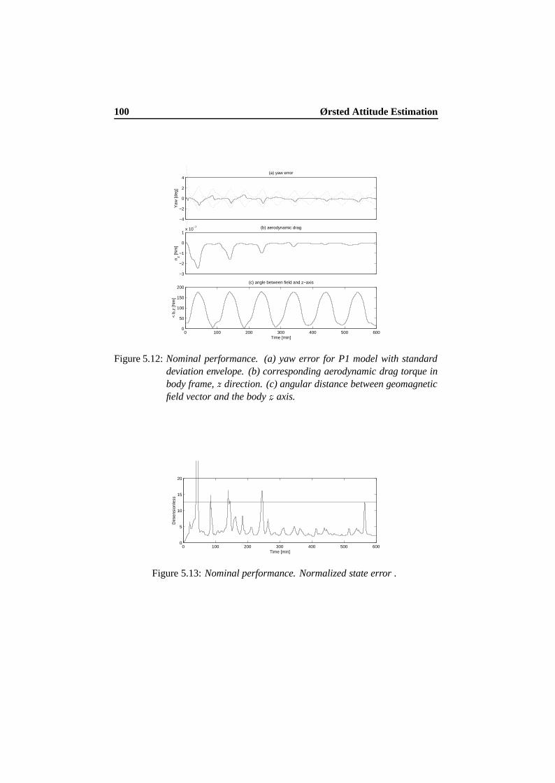
100 Ørsted Attitude Estimation
−4
−2
0
2
4(a) yaw error
Yaw
[deg
]
0 100 200 300 400 500 6000
50
100
150
200
< b
,z [N
m]
Time [min]
(c) angle between field and z−axis
−3
−2
−1
0
1x 10
−7 (b) aerodynamic drag
n z [Nm
]
Figure 5.12: Nominal performance. (a) yaw error for P1 model with standarddeviation envelope. (b) corresponding aerodynamic drag torque inbody frame, ; direction. (c) angular distance between geomagneticfield vector and the body ; axis.
0 100 200 300 400 500 6000
5
10
15
20
Dim
ensi
onle
ss
Time [min]
Figure 5.13: Nominal performance. Normalized state error .
5.5 Performance Analysis for Secondary Operation 101
Fortmann (1988)) a¯´Ä�³ � ¸¤ Õ ¥ ¯ Y » ¥ ¸¤ ¥ (5.19)
where¸¤ ¥ is the error in
�¤ . Under the hypothesis that the estimated covarianceand the true covariance match, the
a¯´Ä�³
is a b  distribution with � degrees offreedom. The � is the state dimension. If the filter is consistent then, by theproperties of this distribution
©«ª a¯´Ä�³W¬ �Í� . The hypothesis is accepted with
95% confidence when the normalized error is below 12.6 since for a six degreeof freedom b  random variable c ª b Âed · �&i ò ¬ ���ai 2 4 .Figure 5.13 plots the normalized error for the nominal performance filter runwith the P1 model. Only 2.5% of the samples are outside the confidence limit at12.6, and it is therefore concluded that the filter is consistent.
Figure 5.13 also shows that the average value lies below the line indicatingthat the filter is conservative – the estimated covariance is larger than the actualmean-squared error of the estimate. This is a direct result of the tuning policy:a conservative design ensures that the filter is robust and consistent. The covari-ance matrix overestimates the errors and so underestimates the accuracy of thefilter. However, it was found that adjusting the noise levels to make the filtermore accurate in this particular case led to inconsistencies in other runs.
The innovations are plotted in Figure 5.14. They are zero mean and boundedby the standard deviations. They are clearly not white, which is a result of thesimplified noise modeling. Periodic field model errors were introduced, but thenoise model assumed a white noise discrepancy. The relative small 7 componentis a result of a generally small 7 component of the geomagnetic field in the orbitframe.
P2 Model Results with the augmented P2 model on the same scenario aregiven in Figure 5.15. The errors in yaw and pitch are reduced as a result ofthe aerodynamic modeling. The reduced stabilizing state noise on the angularvelocity results in lower variance bounds and thereby more confidence in thedynamic model.
The errors in Figure 5.15 are approximately pitch: 0.07 deg. (RMS), roll: 0.1deg. (RMS) and yaw: 0.28 deg. (RMS). The rate errors are ö » : �ai^M<� · � Y`_ rad/sec(RMS), ö Â : �ai Ë �'� · � Y`_ rad/sec (RMS), and ö Î : · i[�û� · � Y`_ rad/sec (RMS). Theangular velocity error are hence reduced especially in ö Â and ö Î , which are thetwo axis that are most affected by aerodynamic drag.
The two estimated components of the aerodynamic drag in the LVLH are
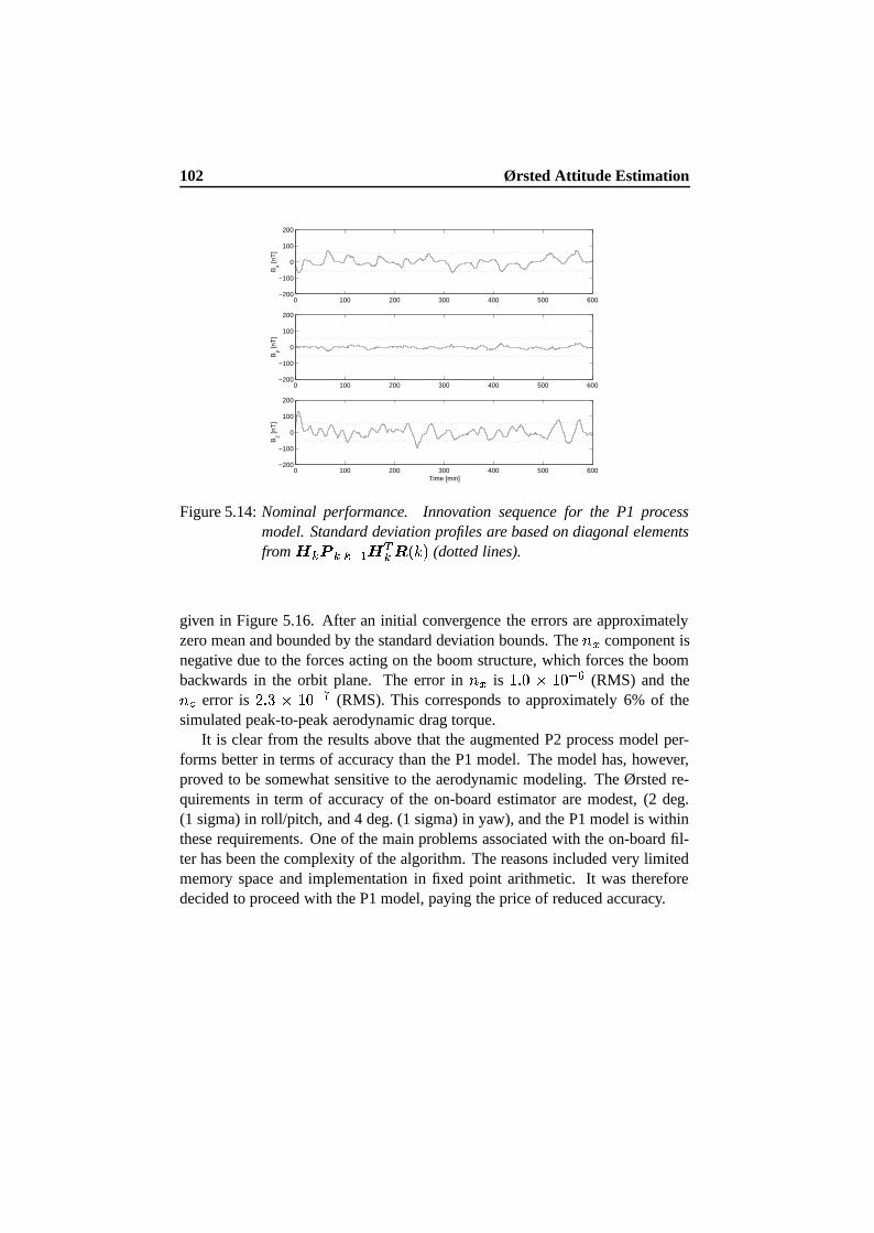
102 Ørsted Attitude Estimation
0 100 200 300 400 500 600−200
−100
0
100
200
Bx [n
T]
0 100 200 300 400 500 600−200
−100
0
100
200
By [n
T]
0 100 200 300 400 500 600−200
−100
0
100
200
Bz [n
T]
Time [min]
Figure 5.14: Nominal performance. Innovation sequence for the P1 processmodel. Standard deviation profiles are based on diagonal elementsfrom à ¯ ¥ Y » Ã Õ ² ¯´Ä�³ (dotted lines).
given in Figure 5.16. After an initial convergence the errors are approximatelyzero mean and bounded by the standard deviation bounds. The � ¾ component isnegative due to the forces acting on the boom structure, which forces the boombackwards in the orbit plane. The error in � ¾ is · i � � · � Y`f (RMS) and the� < error is �&i Ë � · � Yhg (RMS). This corresponds to approximately 6% of thesimulated peak-to-peak aerodynamic drag torque.
It is clear from the results above that the augmented P2 process model per-forms better in terms of accuracy than the P1 model. The model has, however,proved to be somewhat sensitive to the aerodynamic modeling. The Ørsted re-quirements in term of accuracy of the on-board estimator are modest, (2 deg.(1 sigma) in roll/pitch, and 4 deg. (1 sigma) in yaw), and the P1 model is withinthese requirements. One of the main problems associated with the on-board fil-ter has been the complexity of the algorithm. The reasons included very limitedmemory space and implementation in fixed point arithmetic. It was thereforedecided to proceed with the P1 model, paying the price of reduced accuracy.
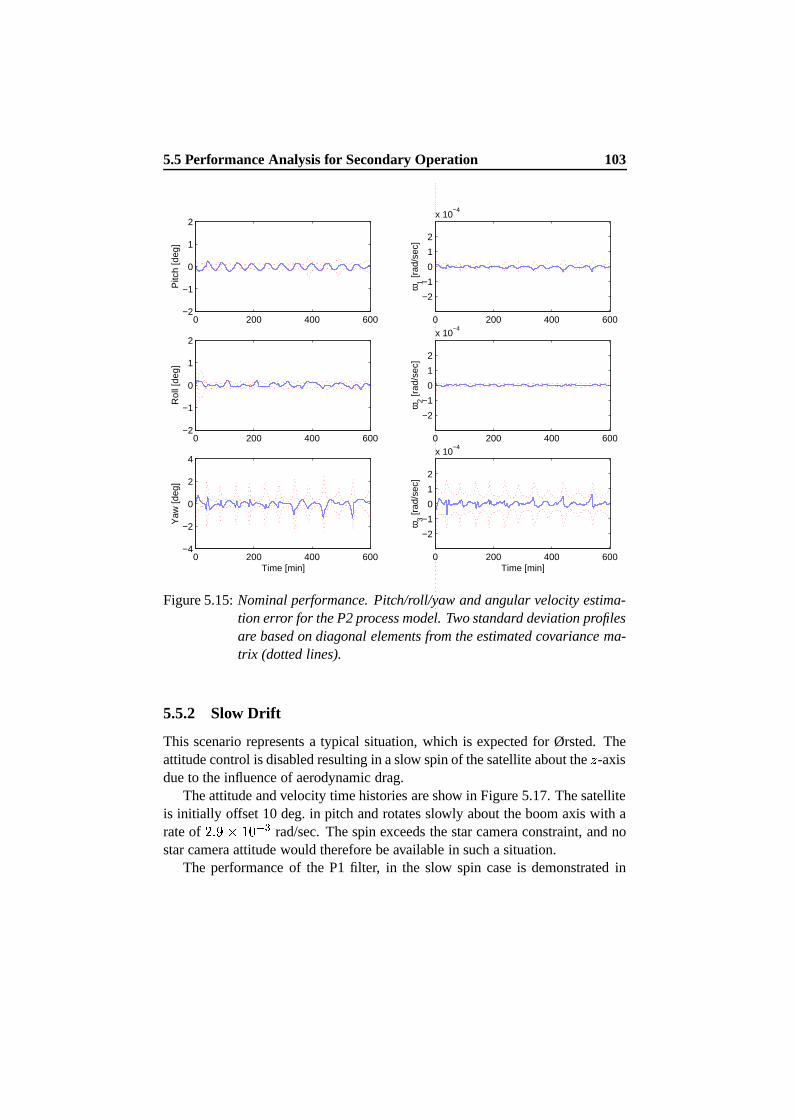
5.5 Performance Analysis for Secondary Operation 103
0 200 400 600−2
−1
0
1
2
Pitc
h [d
eg]
0 200 400 600−2
−1
0
1
2
Rol
l [de
g]
0 200 400 600−4
−2
0
2
4
Yaw
[deg
]
Time [min]
0 200 400 600
−2
−1
0
1
2
x 10−4
ω1 [r
ad/s
ec]
0 200 400 600
−2
−1
0
1
2
x 10−4
ω2 [r
ad/s
ec]
0 200 400 600
−2
−1
0
1
2
x 10−4
ω3 [r
ad/s
ec]
Time [min]
Figure 5.15: Nominal performance. Pitch/roll/yaw and angular velocity estima-tion error for the P2 process model. Two standard deviation profilesare based on diagonal elements from the estimated covariance ma-trix (dotted lines).
5.5.2 Slow Drift
This scenario represents a typical situation, which is expected for Ørsted. Theattitude control is disabled resulting in a slow spin of the satellite about the ; -axisdue to the influence of aerodynamic drag.
The attitude and velocity time histories are show in Figure 5.17. The satelliteis initially offset 10 deg. in pitch and rotates slowly about the boom axis with arate of �&i 2 � · � Y Î rad/sec. The spin exceeds the star camera constraint, and nostar camera attitude would therefore be available in such a situation.
The performance of the P1 filter, in the slow spin case is demonstrated in
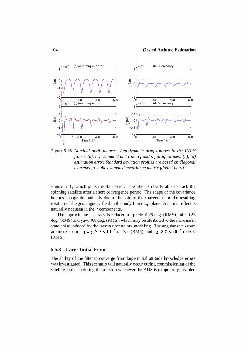
104 Ørsted Attitude Estimation
0 200 400 600−2
−1
0
1x 10
−5
n x [Nm
]
(a) Aero. torque in orbit
0 200 400 600−2
−1
0
1
2x 10
−6
n z [Nm
]
Time [min]
(c) Aero. torque in orbit0 200 400 600
−1
0
1x 10
−5
n x [Nm
]
(b) Discrepancy
0 200 400 600−1
−0.5
0
0.5
1x 10
−6
n z [Nm
]
Time [min]
(d) Discrepancy
Figure 5.16: Nominal performance. Aerodynamic drag torques in the LVLHframe. (a), (c) estimated and true � ¾ and �=< drag torques. (b), (d)estimation error. Standard deviation profiles are based on diagonalelements from the estimated covariance matrix (dotted lines).
Figure 5.18, which plots the state error. The filter is clearly able to track thespinning satellite after a short convergence period. The shape of the covariancebounds change dramatically due to the spin of the spacecraft and the resultingrotation of the geomagnetic field in the body frame > 7 plane. A similar effect isnaturally not seen in the ; components.
The approximate accuracy is reduced to; pitch: 0.26 deg. (RMS), roll: 0.23deg. (RMS) and yaw: 0.8 deg. (RMS), which may be attributed to the increase instate noise induced by the inertia uncertainty modeling. The angular rate errorsare increased to ö » Ö ö Â : �&i 2 � · � Y`_ rad/sec (RMS), and ö Î : �&i^Mý� · � Y`_ rad/sec(RMS).
5.5.3 Large Initial Error
The ability of the filter to converge from large initial attitude knowledge errorswas investigated. This scenario will naturally occur during commissioning of thesatellite, but also during the mission whenever the ADS is temporarily disabled
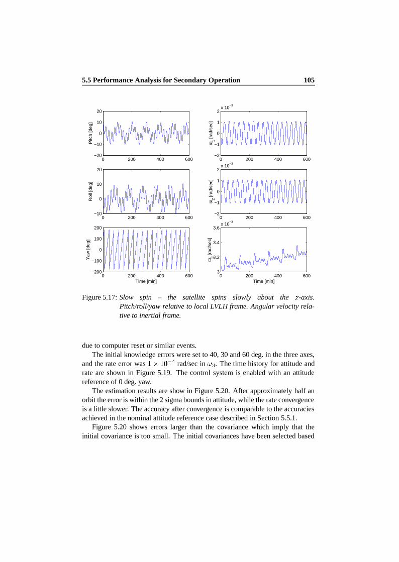
5.5 Performance Analysis for Secondary Operation 105
0 200 400 600−20
−10
0
10
20
Pitc
h [d
eg]
0 200 400 600−10
0
10
20
Rol
l [de
g]
0 200 400 600−200
−100
0
100
200
Yaw
[deg
]
Time [min]
0 200 400 600−2
−1
0
1
2x 10
−3
ω1 [r
ad/s
ec]
0 200 400 600−2
−1
0
1
2x 10
−3
ω2 [r
ad/s
ec]
0 200 400 6003
3.2
3.4
3.6x 10
−3
ω3 [r
ad/s
ec]
Time [min]
Figure 5.17: Slow spin – the satellite spins slowly about the ; -axis.Pitch/roll/yaw relative to local LVLH frame. Angular velocity rela-tive to inertial frame.
due to computer reset or similar events.The initial knowledge errors were set to 40, 30 and 60 deg. in the three axes,
and the rate error was · � · � Y > rad/sec in ö Î . The time history for attitude andrate are shown in Figure 5.19. The control system is enabled with an attitudereference of 0 deg. yaw.
The estimation results are show in Figure 5.20. After approximately half anorbit the error is within the 2 sigma bounds in attitude, while the rate convergenceis a little slower. The accuracy after convergence is comparable to the accuraciesachieved in the nominal attitude reference case described in Section 5.5.1.
Figure 5.20 shows errors larger than the covariance which imply that theinitial covariance is too small. The initial covariances have been selected based
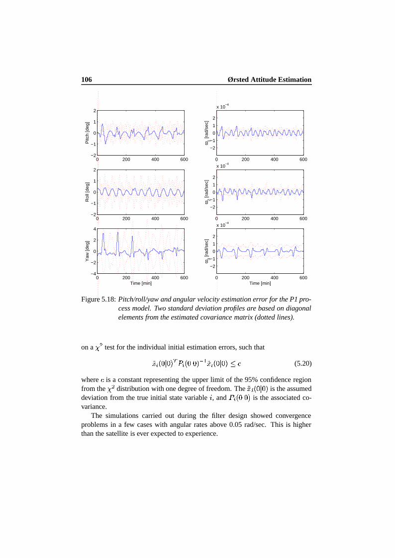
106 Ørsted Attitude Estimation
0 200 400 600−2
−1
0
1
2
Pitc
h [d
eg]
0 200 400 600−2
−1
0
1
2
Rol
l [de
g]
0 200 400 600−4
−2
0
2
4
Yaw
[deg
]
Time [min]
0 200 400 600
−2
−1
0
1
2
x 10−4
ω1 [r
ad/s
ec]
0 200 400 600
−2
−1
0
1
2
x 10−4
ω2 [r
ad/s
ec]
0 200 400 600
−2
−1
0
1
2
x 10−4
ω3 [r
ad/s
ec]
Time [min]
Figure 5.18: Pitch/roll/yaw and angular velocity estimation error for the P1 pro-cess model. Two standard deviation profiles are based on diagonalelements from the estimated covariance matrix (dotted lines).
on a b  test for the individual initial estimation errors, such that¸>�¡ ¯ � µ � ³ Õ c¼¡ ¯ � µ � ³ Y » ¸>�¡ ¯ � µ � ³ dji (5.20)
where i is a constant representing the upper limit of the 95% confidence regionfrom the b  distribution with one degree of freedom. The
¸>D¡ ¯ � µ � ³ is the assumeddeviation from the true initial state variable
ñ, and c¶¡ ¯ � µ � ³ is the associated co-
variance.The simulations carried out during the filter design showed convergence
problems in a few cases with angular rates above 0.05 rad/sec. This is higherthan the satellite is ever expected to experience.
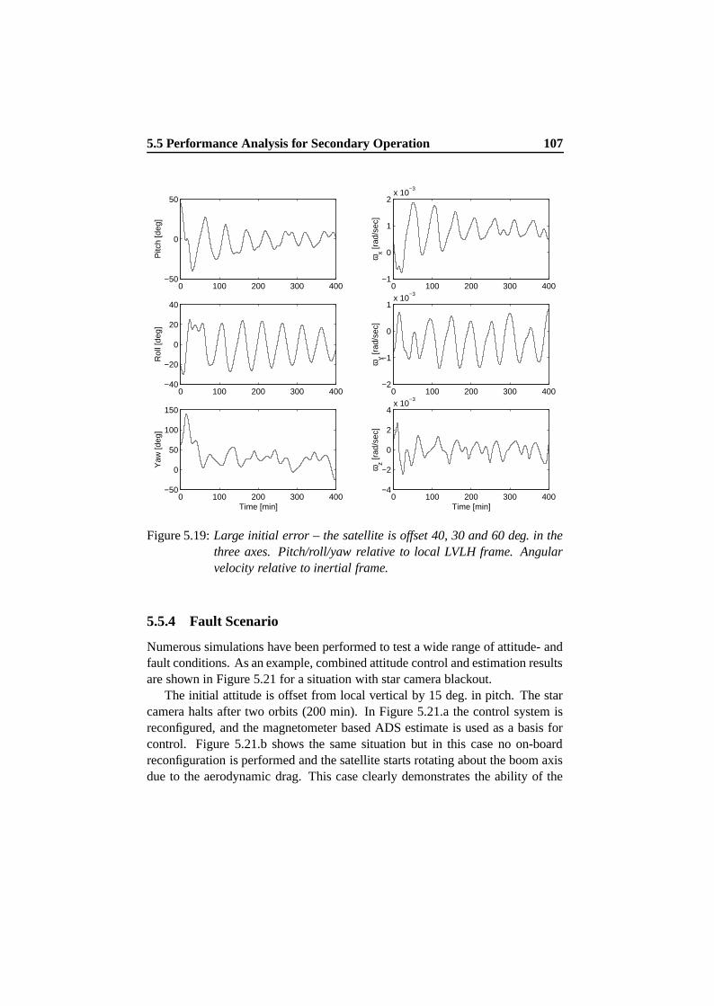
5.5 Performance Analysis for Secondary Operation 107
0 100 200 300 400−50
0
50
Pitc
h [d
eg]
0 100 200 300 400−40
−20
0
20
40
Rol
l [de
g]
0 100 200 300 400−50
0
50
100
150
Yaw
[deg
]
Time [min]
0 100 200 300 400−1
0
1
2x 10
−3
ωx [r
ad/s
ec]
0 100 200 300 400−2
−1
0
1x 10
−3
ωy [r
ad/s
ec]
0 100 200 300 400−4
−2
0
2
4x 10
−3
ωz [r
ad/s
ec]
Time [min]
Figure 5.19: Large initial error – the satellite is offset 40, 30 and 60 deg. in thethree axes. Pitch/roll/yaw relative to local LVLH frame. Angularvelocity relative to inertial frame.
5.5.4 Fault Scenario
Numerous simulations have been performed to test a wide range of attitude- andfault conditions. As an example, combined attitude control and estimation resultsare shown in Figure 5.21 for a situation with star camera blackout.
The initial attitude is offset from local vertical by 15 deg. in pitch. The starcamera halts after two orbits (200 min). In Figure 5.21.a the control system isreconfigured, and the magnetometer based ADS estimate is used as a basis forcontrol. Figure 5.21.b shows the same situation but in this case no on-boardreconfiguration is performed and the satellite starts rotating about the boom axisdue to the aerodynamic drag. This case clearly demonstrates the ability of the
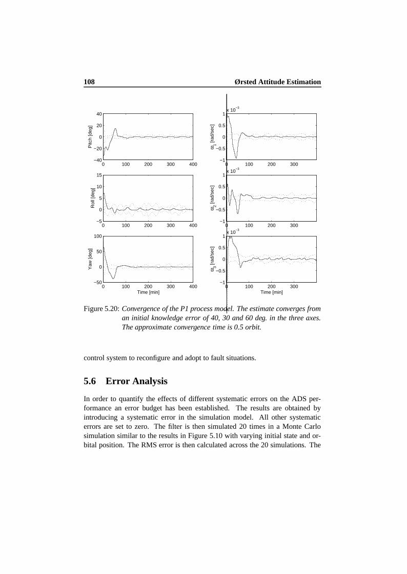
108 Ørsted Attitude Estimation
0 100 200 300 400−40
−20
0
20
40
Pitc
h [d
eg]
0 100 200 300 400−5
0
5
10
15
Rol
l [de
g]
0 100 200 300 400−50
0
50
100
Yaw
[deg
]
Time [min]
0 100 200 300−1
−0.5
0
0.5
1x 10
−3
ω1 [r
ad/s
ec]
0 100 200 300−1
−0.5
0
0.5
1x 10
−3
ω2 [r
ad/s
ec]
0 100 200 300−1
−0.5
0
0.5
1x 10
−3
ω3 [r
ad/s
ec]
Time [min]
Figure 5.20: Convergence of the P1 process model. The estimate converges froman initial knowledge error of 40, 30 and 60 deg. in the three axes.The approximate convergence time is 0.5 orbit.
control system to reconfigure and adopt to fault situations.
5.6 Error Analysis
In order to quantify the effects of different systematic errors on the ADS per-formance an error budget has been established. The results are obtained byintroducing a systematic error in the simulation model. All other systematicerrors are set to zero. The filter is then simulated 20 times in a Monte Carlosimulation similar to the results in Figure 5.10 with varying initial state and or-bital position. The RMS error is then calculated across the 20 simulations. The
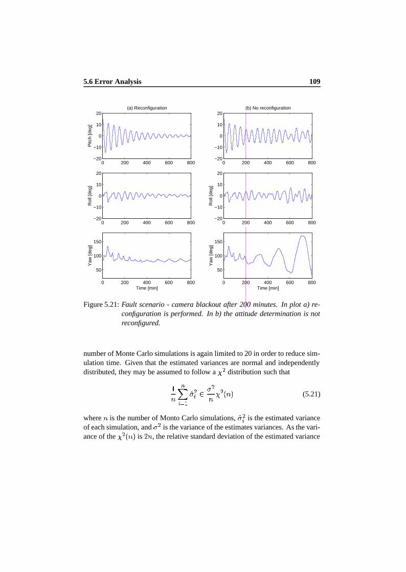
5.6 Error Analysis 109
0 200 400 600 800−20
−10
0
10
20
Pitc
h [d
eg]
(a) Reconfiguration
0 200 400 600 800−20
−10
0
10
20
Rol
l [de
g]
0 200 400 600 800
50
100
150
Yaw
[deg
]
Time [min]
0 200 400 600 800−20
−10
0
10
20(b) No reconfiguration
0 200 400 600 800−20
−10
0
10
20
Rol
l [de
g]
0 200 400 600 800
50
100
150
Yaw
[deg
]
Time [min]
Figure 5.21: Fault scenario - camera blackout after 200 minutes. In plot a) re-configuration is performed. In b) the attitude determination is notreconfigured.
number of Monte Carlo simulations is again limited to 20 in order to reduce sim-ulation time. Given that the estimated variances are normal and independentlydistributed, they may be assumed to follow a b  distribution such that
·�¸¹¡Ñº¼»
�1 ¡ Æk1 Â� b  ¯ � ³ (5.21)
where � is the number of Monto Carlo simulations,�1 ¡ is the estimated variance
of each simulation, and 1  is the variance of the estimates variances. As the vari-ance of the b  ¯ � ³ is �E� , the relative standard deviation of the estimated variance
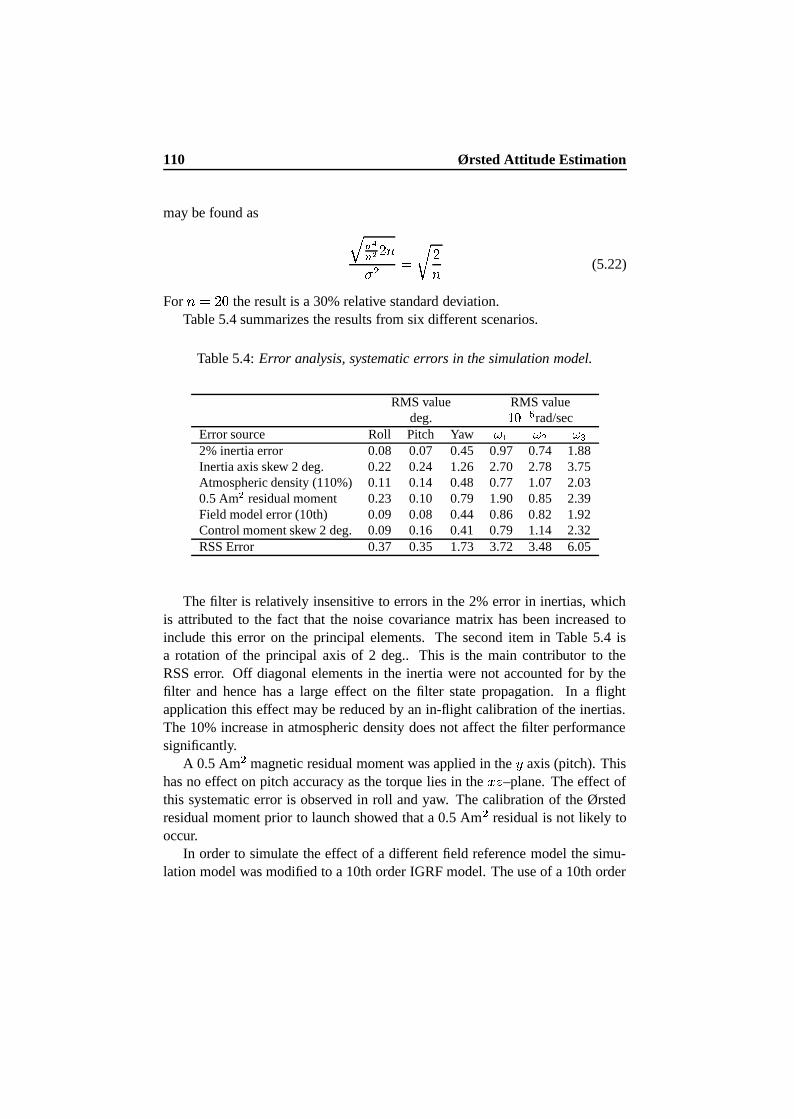
110 Ørsted Attitude Estimation
may be found as î GQl¸ # �E�1  �nm �� (5.22)
For �ª� �]� the result is a 30% relative standard deviation.Table 5.4 summarizes the results from six different scenarios.
Table 5.4: Error analysis, systematic errors in the simulation model.
RMS value RMS valuedeg. &*) �SX rad/sec
Error source Roll Pitch Yaw � � � � 2% inertia error 0.08 0.07 0.45 0.97 0.74 1.88Inertia axis skew 2 deg. 0.22 0.24 1.26 2.70 2.78 3.75Atmospheric density (110%) 0.11 0.14 0.48 0.77 1.07 2.030.5 Am residual moment 0.23 0.10 0.79 1.90 0.85 2.39Field model error (10th) 0.09 0.08 0.44 0.86 0.82 1.92Control moment skew 2 deg. 0.09 0.16 0.41 0.79 1.14 2.32RSS Error 0.37 0.35 1.73 3.72 3.48 6.05
The filter is relatively insensitive to errors in the 2% error in inertias, whichis attributed to the fact that the noise covariance matrix has been increased toinclude this error on the principal elements. The second item in Table 5.4 isa rotation of the principal axis of 2 deg.. This is the main contributor to theRSS error. Off diagonal elements in the inertia were not accounted for by thefilter and hence has a large effect on the filter state propagation. In a flightapplication this effect may be reduced by an in-flight calibration of the inertias.The 10% increase in atmospheric density does not affect the filter performancesignificantly.
A 0.5 Am  magnetic residual moment was applied in the 7 axis (pitch). Thishas no effect on pitch accuracy as the torque lies in the >o; –plane. The effect ofthis systematic error is observed in roll and yaw. The calibration of the Ørstedresidual moment prior to launch showed that a 0.5 Am  residual is not likely tooccur.
In order to simulate the effect of a different field reference model the simu-lation model was modified to a 10th order IGRF model. The use of a 10th order
5.7 Summary 111
model seems to have little effect on the filter performance. As it was seen inFigure 5.6 the variance of the 10th order model compared to the 8th order modelis lower than the variance of the field model discrepancies used in the nominalsimulation model. From this it is clear that the current measurement noise cov-ers the systematic error introduced by using the 10th order model. The analysisshows that filter is not sensitive to the changes in frequency of the reference fieldmodel.
Finally a 2 deg. rotation was applied to the control moment vector, whichonly has limited effect on the accuracy. This is mainly due to the relative lowmagnetic control moment ( � � ÏÑÐ:� d �ai ò Am  ) generated during the scenario inFigure 5.10.
The root square sum (RSS) in Table 5.4 indicate an expected accuracy ofapproximately 0.37 and 0.34 deg. in pitch and roll and 1.73 in yaw. The RSSerrors in angular velocity are approximately
Ë i^M �©� · � Y`_ rad/sec in ö » , Ë i[� h �· � Y`_ rad/sec in ö  and finally error is ò i �p4� · � Y`_ rad/sec. This result is wellbelow the specifications in angles and marginally below the specification in theangular rates. Even with the 30% relative standard deviations on the results doesnot violate specifications.
5.7 Summary
The objective of this chapter has been to develop an ADS for estimation of three-axis spacecraft attitude and rate information, based solely on three-axis magne-tometer measurements.
A system for estimating three-axis spacecraft attitude and rates by Kalmanfiltering of magnetometer data has been described. The Kalman filter estimatesare supplementing star camera based estimates. The two estimation algorithmsoperate in parallel providing fault tolerance towards Sun sensor and star camerablackouts. Combined with detection algorithms the presented attitude determi-nation introduces a significant degree of autonomy.
Section 5.1 presented the motivation and problems associated with the ADS,which has been incorporated in the attitude control system for the Ørsted satel-lite. Section 5.2 addressed the requirements to the ADS while Section 5.3 de-scribed the simulation model which is the basis for tests of the estimator design.Two process models were presented in Section 5.4 and their noise parametersspecified.
In Section 5.5 the simulated results of the actively controlled, zenith pointing

112 Ørsted Attitude Estimation
spacecraft demonstrated the ability of the estimation algorithm. With the sys-tem described, sufficient in-flight attitude estimation accuracy is maintained forattitude control purposes. Finally Section 5.6 presented an error budget whichcombines the effects of a number of systematic errors. The attitude determi-nation based on magnetometer data only was found effective and the obtainedaccuracies were 0.37-0.34 deg. in pitch/roll, 1.73 deg. in yaw. The angular rateaccuracies were found to be ö » : Ë i^M �3� · � Y`_ rad/sec, ö Â : Ë i[� h � · � Y`_ rad/sec,and finally ö Î : ò i �p4(� · � Y`_ rad/sec. A 30% standard deviation is estimated onthese results.
Chapter 6
Implementation and Resultsfrom Ørsted
It is well–known that the Kalman filter in its original formulation is sensitive tonumerical inaccuracy and the extended Kalman filter has potential instability. Asthe Kalman filter described in the previous chapter is developed for implementa-tion in the on-board computer of the Ørsted satellite the numerical behaviour ofthe algorithm has to be addressed. Section 6.1 gives a brief description of the is-sues related to a fixed point Ada implementation for Ørsted. Section 6.2 presentsresults from the on board ADS. The results from the magnetometer based esti-mation of attitude are compared to star camera attitudes thereby providing anassessment of the absolute accuracy.
6.1 Implementation
Up to this point the discussion has focused on a theoretical performance of theKalman filter using given truth models for simulations. It is, however, well–known that the Kalman filter in its original formulation may predict results thatdiffer from observed behaviour. This difference or divergence may be causedby: modeling errors, poor state observability, and numerical inaccuracy. Thissection focuses on the numerical issue.
The Ørsted on-board software and thereby the control system was imple-mented using the Ada programming language. This choice was not necessarilywise when considering numerical intensive algorithms, but Ada provide othersoftware engineering benefits like readability, maintainability, portability, etc.
113
114 Implementation and Results from Ørsted
that were important for the project development.The Kalman filter is evaluated in the on-board processor as a real time pro-
cess, implying that the filter has to perform the necessary calculations betweensamples. As the sampling time is relative low (10 seconds) this is not a severeconstraint. The main practical constraints were caused by the fixed point arith-metic and the code size.
6.1.1 Core Numerical Algorithms
The main problem with a fixed point implementation is the reduced dynamicrange imposed by the arithmetic, which may lead to divergence of the filter.The internal data flow in the Kalman filter consists basically of two estimationloops. The estimated mean (state estimate) is propagated around one loop, andthe covariance in another.
– In the state estimation loop, errors in the estimated mean introduced byroundoff and noise are compensated by feedback through the weighted(Kalman gain) innovation.
– The covariance loop is not stabilized by feedback, and as a result, errorspropagate and accumulate. This may lead to errors in the mean estimateand divergence of the filter. The computations involved in the covarianceprediction must therefore be addressed.
Implementation methods for reducing the effects of roundoff errors in the co-variance loop have been intensely studied since the numerical difficulties withthe Kalman filter were first addressed in the mid seventies. The most success-ful and numerical stable implementations are based on the idea of propagatingsymmetric products of triangular factors for the covariance matrix, rather thatthe covariance matrix itself (Grewal and Andrews (1993)).
The Ørsted ADS employs a covariance formulation, which is based on amodified Cholesky decomposition (UD decomposition) of the covariance ma-trix. This formulation provides adequate covariance matrix precision with singleprecision fixed-point arithmetic.
The measurement update is done using Bierman’s Square Root Free squareroot observational update (Bierman (1977)), and the covariance time updateis based on Thornton’s modified weighted Gram-Schmidt algorithm (Thornton(1976)). These methods belong among the most numerically stable algorithmsfor Kalman filter implementation (Grewal and Andrews (1993)).
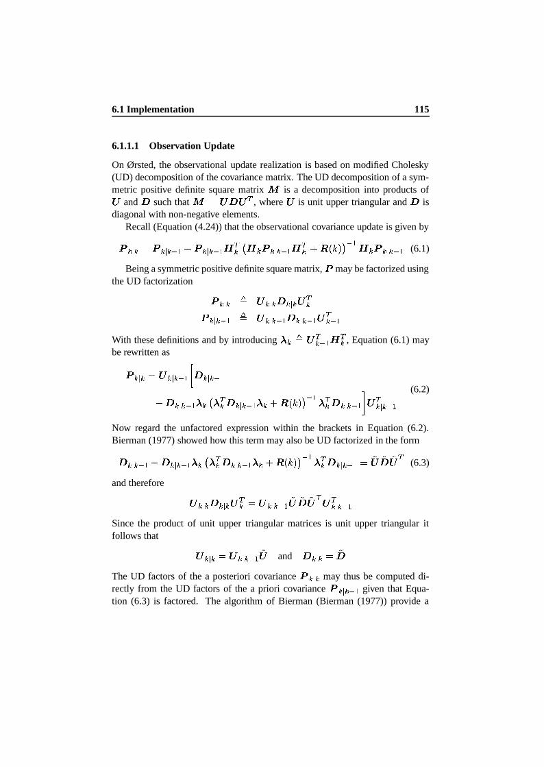
6.1 Implementation 115
6.1.1.1 Observation Update
On Ørsted, the observational update realization is based on modified Cholesky(UD) decomposition of the covariance matrix. The UD decomposition of a sym-metric positive definite square matrix q is a decomposition into products ofr
and s such that q � r s r Õ , wherer
is unit upper triangular and s isdiagonal with non-negative elements.
Recall (Equation (4.24)) that the observational covariance update is given by¯ ¥ �Q¯ ¥ Y » �"¯ ¥ Y » Ã Õ » à ¯ ¥ Y » Ã Õ £<² ¯´Ä�³ ½ Y » à ¯ ¥ Y » (6.1)
Being a symmetric positive definite square matrix, ¯ may be factorized usingthe UD factorization ¯ ¥ µ r ¥ s ¥ r Õ ¯ ¥ Y » µ r ¥ Y » s ¥ Y » r Õ Y »With these definitions and by introducing t µur Õ Y » Ã Õ , Equation (6.1) maybe rewritten as¯ ¥ � r ¥ Y » @ s ¥ Y »�vs ¥ Y » t »&t Õ s ¥ Y » t £S² ¯´Ä�³ ½ Y » t Õ s ¥ Y » B r Õ ¥ Y » (6.2)
Now regard the unfactored expression within the brackets in Equation (6.2).Bierman (1977) showed how this term may also be UD factorized in the forms ¥ Y » �ws ¥ Y » t »xt Õ s ¥ Y » t £S² ¯´Ä�³ ½ Y » t Õ s ¥ Y » � ¸r ¸s ¸r Õ (6.3)
and therefore r ¥ s ¥ r Õ � r ¥ Y » ¸r ¸s ¸r Õ r Õ ¥ Y »Since the product of unit upper triangular matrices is unit upper triangular itfollows that r ¥ � r ¥ Y » ¸r and s ¥ � ¸sThe UD factors of the a posteriori covariance ¯ ¥ may thus be computed di-rectly from the UD factors of the a priori covariance ¯ ¥ Y » given that Equa-tion (6.3) is factored. The algorithm of Bierman (Bierman (1977)) provide a
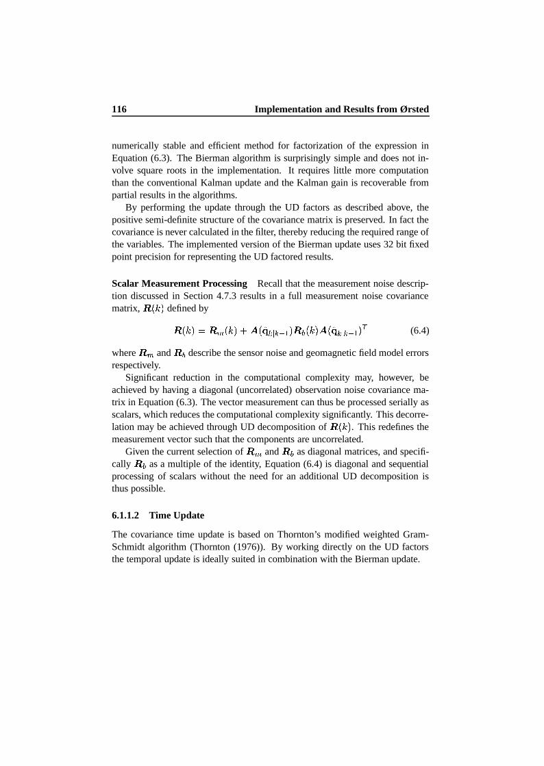
116 Implementation and Results from Ørsted
numerically stable and efficient method for factorization of the expression inEquation (6.3). The Bierman algorithm is surprisingly simple and does not in-volve square roots in the implementation. It requires little more computationthan the conventional Kalman update and the Kalman gain is recoverable frompartial results in the algorithms.
By performing the update through the UD factors as described above, thepositive semi-definite structure of the covariance matrix is preserved. In fact thecovariance is never calculated in the filter, thereby reducing the required range ofthe variables. The implemented version of the Bierman update uses 32 bit fixedpoint precision for representing the UD factored results.
Scalar Measurement Processing Recall that the measurement noise descrip-tion discussed in Section 4.7.3 results in a full measurement noise covariancematrix, ² ¯´Ä�³ defined by² ¯´Ä�³ �Q² ø ¯´Ä�³ £ ± ¯Á�5 ¥ Y » ³ ² Ú ¯´Ä�³W±«¯Á�
5 ¥ Y » ³ Õ (6.4)
where ²¿ø and ² Ú describe the sensor noise and geomagnetic field model errorsrespectively.
Significant reduction in the computational complexity may, however, beachieved by having a diagonal (uncorrelated) observation noise covariance ma-trix in Equation (6.3). The vector measurement can thus be processed serially asscalars, which reduces the computational complexity significantly. This decorre-lation may be achieved through UD decomposition of ² ¯´Ä�³ . This redefines themeasurement vector such that the components are uncorrelated.
Given the current selection of ²çø and ² Ú as diagonal matrices, and specifi-cally ² Ú as a multiple of the identity, Equation (6.4) is diagonal and sequentialprocessing of scalars without the need for an additional UD decomposition isthus possible.
6.1.1.2 Time Update
The covariance time update is based on Thornton’s modified weighted Gram-Schmidt algorithm (Thornton (1976)). By working directly on the UD factorsthe temporal update is ideally suited in combination with the Bierman update.
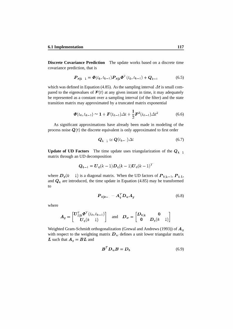
6.1 Implementation 117
Discrete Covariance Prediction The update works based on a discrete timecovariance prediction, that is¯ ¥ Y » ��Õ ¯lk Ö8k Y » ³ ¯ ¥ Õ Õ ¯lk Ö8k Y » ³ £<¨ Y » (6.5)
which was defined in Equation (4.85). As the sampling interval m k is small com-pared to the eigenvalues of ¡ ¯lk�³ at any given instant in time, it may adequatelybe represented as a constant over a sampling interval (of the filter) and the statetransition matrix may approximated by a truncated matrix exponentialÕ ¯lk Ö8k Y » ³ Û �ï£<¡ ¯lk Y » ³ m k £ ·
� ¡  ¯lk Y » ³ m k  (6.6)
As significant approximations have already been made in modeling of theprocess noise ¨ ¯lkt³ the discrete equivalent is only approximated to first order¨ Y » Û ¨ ¯lk Y » ³ m k (6.7)
Update of UD Factors The time update uses triangularization of the ¨ Y »matrix through an UD decomposition¨ Y » � r ã ¯´Ä � · ³ s®ã ¯´Ä � · ³"r ã ¯´Ä � · ³ Õwhere s"ã ¯´Ä � · ³ is a diagonal matrix. When the UD factors of ¯ ¥ Y » , ¯ ¥ ,and ¨ are introduced, the time update in Equation (4.85) may be transformedto ¯ ¥ Y » � ± Õ � s D ± � (6.8)
where
± ��� @ r Õ ¥ Õ Õ ¯lk Ö8k Y » ³r ã ¯´Ä � · ³ B and s D � @ s ¥ RR s ã ¯´Ä � · ³ BWeighted Gram-Schmidt orthogonalization (Grewal and Andrews (1993)) of
± �with respect to the weighting matrix s D defines a unit lower triangular matrixy
such that± ��� � y and
� Õ s D ���Fs Ú (6.9)
118 Implementation and Results from Ørsted
where s Ú is a diagonal matrix representing the fact that the column vectors of� are orthogonal with respect to s D 1. Using the result of the weighted Gram-Schmidt orthogonalization, Equation (6.8) may be reformulated as¯ ¥ Y » � y Õ¼�¢Õ�s D � y
� y Õ�s Ú y (6.10)
As UD factorization is unique, andy
is unit lower triangular and s Ú diagonalthe temporal update of the UD factored covariance is given byr ¥ Y » � y Õ and s ¥ Y » �Fs Ú (6.11)
This is used directly in the measurement update outlined above. The covariancesare thus never directly calculated in the real-time implementation. The combinedcovariance prediction implemented on Ørsted is shown in Figure 6.1.
Figure 6.1: Schematically overview of the covariance prediction implemented onØrsted. Bierman’s square root free measurement update is combinedwith Thornton’s temporal update .
1The vectors ý and z are said to be orthogonal with respect to {J| if the weighted innerproduct ý íC{}|Vz�ì�~ .
6.1 Implementation 119
6.1.2 Reference Field Implementation
Another computationally complex algorithm is the IGRF reference field modelrequired for the measurement update. A 16 bit fixed point Ada implementationwas established based on a standard IGRF Fortran model. The algorithm wastested over a wide range of possible orbital positions and the results comparedwith results from a floating point implementation in Matlab. The errors commit-ted by this low accuracy implementation were found to be approximately 30 nT(RMS) as shown in Figure 6.2. This is acceptable as the modeling error inher-ent to the IGRF model was found in Section 5.3.2.1 to be approximately 83 nT(RMS) when compared to data from Freja.
0 10 20 30 40 50 60 70 80 90 100−100
−50
0
50
100Discrepancy Ada/Matlab
nT
Samples
Figure 6.2: On-board geomagnetic field model. Three components of the refer-ence field in orbital positions distributed over 24 hours. Discrepancybetween Ada fixed point implementation and Matlab 8th order model.
6.1.3 ADS Implementation in Software
The Ørsted ADS has been implemented as a task running on one of the two on-board computers. The ADS software is executed as part of the central controllevel task. The interaction of the control level task with other ACS tasks is shownin Figure 6.3.
The control level task runs at a 10 second cycle that can be interrupted bya synchronous rendezvous with reconfiguration commands from a parallel run-ning supervisor task. The preprocessed magnetometer readings are generatedafter an interrupt from the control level task and are transferred synchronouslythrough rendezvous with an input dispatcher task that handles the interface tothe other subsystems. The variables required for integrity monitoring and faultdetection are transferred asynchronously from the control task to the supervisortask through a variable pool that is protected by a semaphore. The internal pa-
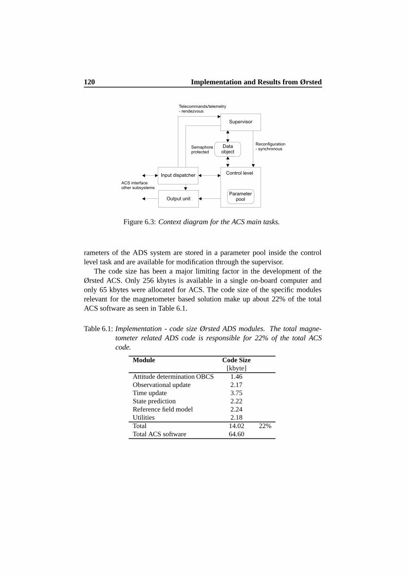
120 Implementation and Results from Ørsted
Figure 6.3: Context diagram for the ACS main tasks.
rameters of the ADS system are stored in a parameter pool inside the controllevel task and are available for modification through the supervisor.
The code size has been a major limiting factor in the development of theØrsted ACS. Only 256 kbytes is available in a single on-board computer andonly 65 kbytes were allocated for ACS. The code size of the specific modulesrelevant for the magnetometer based solution make up about 22% of the totalACS software as seen in Table 6.1.
Table 6.1: Implementation - code size Ørsted ADS modules. The total magne-tometer related ADS code is responsible for 22% of the total ACScode.
Module Code Size[kbyte]
Attitude determination OBCS 1.46Observational update 2.17Time update 3.75State prediction 2.22Reference field model 2.24Utilities 2.18Total 14.02 22%Total ACS software 64.60
6.2 Results from Ørsted 121
The module Attitude determination OBCS (Object Control Structure) exe-cutes the overall control of the ADS, which involves transitions between sec-ondary (magnetometer) and primary sensors (star camera). The main burden isassociated with the time update which involves the modules time update and stateprediction. The module utilities provided services such as multiplication to theother modules. The total execution time of the ACS control task, which involvethe attitude determination has been measured to 1.788 sec (Bøgh (1996). Witha nominal cycle time of 10 seconds the ACS is hence responsible for about 18%of the computational load on the computer where the ACS software is running.
6.2 Results from Ørsted
With the launch of Ørsted on February 23, 1999, data are available for evaluationof the on-board estimation algorithm. Investigation are still ongoing, and theresults presented here are considered preliminary.
As with most other satellites a number of difficulties have been discovered inrelation to the flight configuration, many of which are yet unsolved. Of primaryconcern to evaluation of the ADS are the following
– Boom distortion. After deployment of the Ørsted boom significant dis-crepancy was found between the expected gondola and actual gondola ori-entation. A calibration based on Sun sensor and star camera data showeda 45 deg. rotation of the gondola relative to nominal. The ADS gondola tobody rotation has been adjusted according to the calibration. The accuracyof the calibration is, however, limited due to the limited accuracy of theSun sensors. This uncertainty is transferred to the ADS as uncertainty inthe moments of inertia, and the control torque input. No explanation forthis unexpected rotation has yet been found.
– Boom flexibility. When torques are applied to the satellite by the con-trol system boom oscillations have been experienced at a frequency muchlower than expected. Thermal effects also have an apparent influence. Onthe day side of the orbit boom oscillations are generated. Each upset of theboom (boom quake) is associated with a change in the boom stiffness, asseen on the eigenfrequency of the associated torsional vibrations (Bauer(1999)). Boom oscillations apparently cause star camera vibrations, andloss of star camera availability for a period of 20–40 sec. This phenom-ena may be coupled to the boom distortion and has so far not been fully
122 Implementation and Results from Ørsted
understood.
– Star camera timing. Timing problems with the star camera complicatesthe use of the star camera quaternion as a reference for evaluating theADS. The timing problem has been solved, but data were only availablefor a very limited part of the mission at the time of writing. The analysispresented here is based on raw star camera attitude estimates.
– Control system torques. Current spikes in the magnetorquers combinedwith rapid changes in the current demands resulted in input torques thatwere problematic for the star camera. In combination with the boom os-cillation phenomena the torque input caused the star camera to generatedegraded estimates and eventually fall out. The problem was minimizedby adjustments of star camera sensitivity and control system parameters,in particular the maximal allowed control current.
– Unknown input torque. The behaviour of the control system before boomdeployment and during normal operation indicates some unknown distur-bance torques. This assumption is supported by the analysis of the estima-tor performance discussed below.
The issues above all make the attitude determination task more difficult andthe results presented in the next section are thus expected to be slightly worsethan could be achieved. As the problems above are solved, the on-board filterwill be adjusted accordingly and the errors may decrease somewhat.
6.2.1 Attitude Time Histories
Two different sets of orbits have been selected for an evaluation of the ADS per-formance. During the first six month of operation only approximately 30% goodstar camera data were available and the control of the satellite hence dependedon the magnetometer based solution for a large part of the time.
The two sets presented here have been selected so that star camera data wereavailable for comparison of the results. The first set represents a typical situationwhere the satellite is rotating slowly about the ; axis, whereas set two representsthe situation as it has been after some adjustments in late August 1999.
Orbits 2535-2538 The attitude estimated by the magnetometer based solutionis compared with available star camera data. The results presented in Figure 6.4are based on four orbits 2535-2538 (August 18 1999 UTC: 12:34:38).
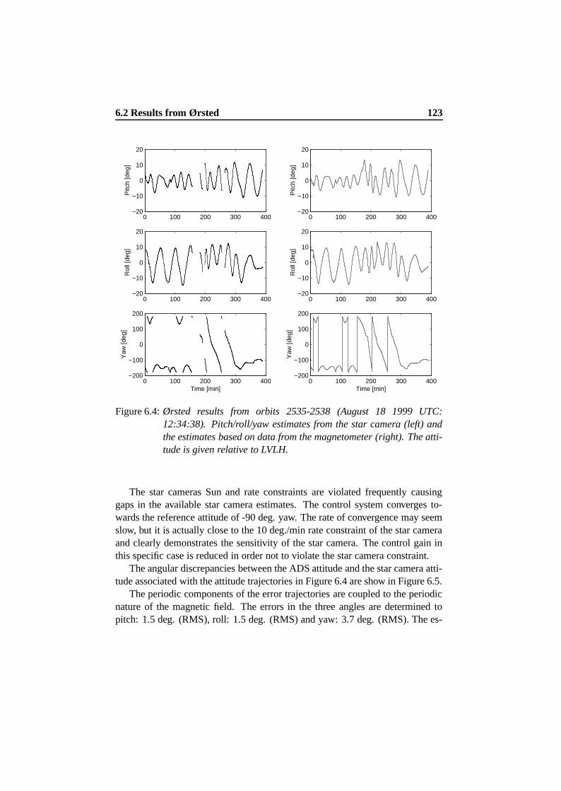
6.2 Results from Ørsted 123
0 100 200 300 400−20
−10
0
10
20
Pitc
h [d
eg]
0 100 200 300 400−20
−10
0
10
20
Rol
l [de
g]
0 100 200 300 400−200
−100
0
100
200
Yaw
[deg
]
Time [min]
0 100 200 300 400−20
−10
0
10
20
Pitc
h [d
eg]
0 100 200 300 400−20
−10
0
10
20
Rol
l [de
g]
0 100 200 300 400−200
−100
0
100
200
Yaw
[deg
]
Time [min]
Figure 6.4: Ørsted results from orbits 2535-2538 (August 18 1999 UTC:12:34:38). Pitch/roll/yaw estimates from the star camera (left) andthe estimates based on data from the magnetometer (right). The atti-tude is given relative to LVLH.
The star cameras Sun and rate constraints are violated frequently causinggaps in the available star camera estimates. The control system converges to-wards the reference attitude of -90 deg. yaw. The rate of convergence may seemslow, but it is actually close to the 10 deg./min rate constraint of the star cameraand clearly demonstrates the sensitivity of the star camera. The control gain inthis specific case is reduced in order not to violate the star camera constraint.
The angular discrepancies between the ADS attitude and the star camera atti-tude associated with the attitude trajectories in Figure 6.4 are show in Figure 6.5.
The periodic components of the error trajectories are coupled to the periodicnature of the magnetic field. The errors in the three angles are determined topitch: 1.5 deg. (RMS), roll: 1.5 deg. (RMS) and yaw: 3.7 deg. (RMS). The es-
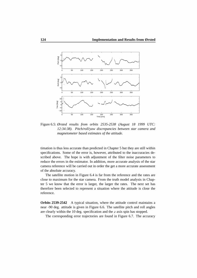
124 Implementation and Results from Ørsted
0 50 100 150 200 250 300 350
−5
0
5
Pitc
h [d
eg]
0 50 100 150 200 250 300 350
−5
0
5
Rol
l [de
g]
0 50 100 150 200 250 300 350
−10
−5
0
5
10
Yaw
[deg
]
Time [min]
Figure 6.5: Ørsted results from orbits 2535-2538 (August 18 1999 UTC:12:34:38). Pitch/roll/yaw discrepancies between star camera andmagnetometer based estimates of the attitude.
timation is thus less accurate than predicted in Chapter 5 but they are still withinspecifications. Some of the error is, however, attributed to the inaccuracies de-scribed above. The hope is with adjustment of the filter noise parameters toreduce the errors in the estimator. In addition, more accurate analysis of the starcamera reference will be carried out in order the get a more accurate assessmentof the absolute accuracy.
The satellite motion in Figure 6.4 is far from the reference and the rates areclose to maximum for the star camera. From the truth model analysis in Chap-ter 5 we know that the error is larger, the larger the rates. The next set hastherefore been selected to represent a situation where the attitude is close thereference.
Orbits 2539-2542 A typical situation, where the attitude control maintains anear -90 deg. attitude is given in Figure 6.6. The satellite pitch and roll anglesare clearly within the 10 deg. specification and the ; axis spin has stopped.
The corresponding error trajectories are found in Figure 6.7. The accuracy
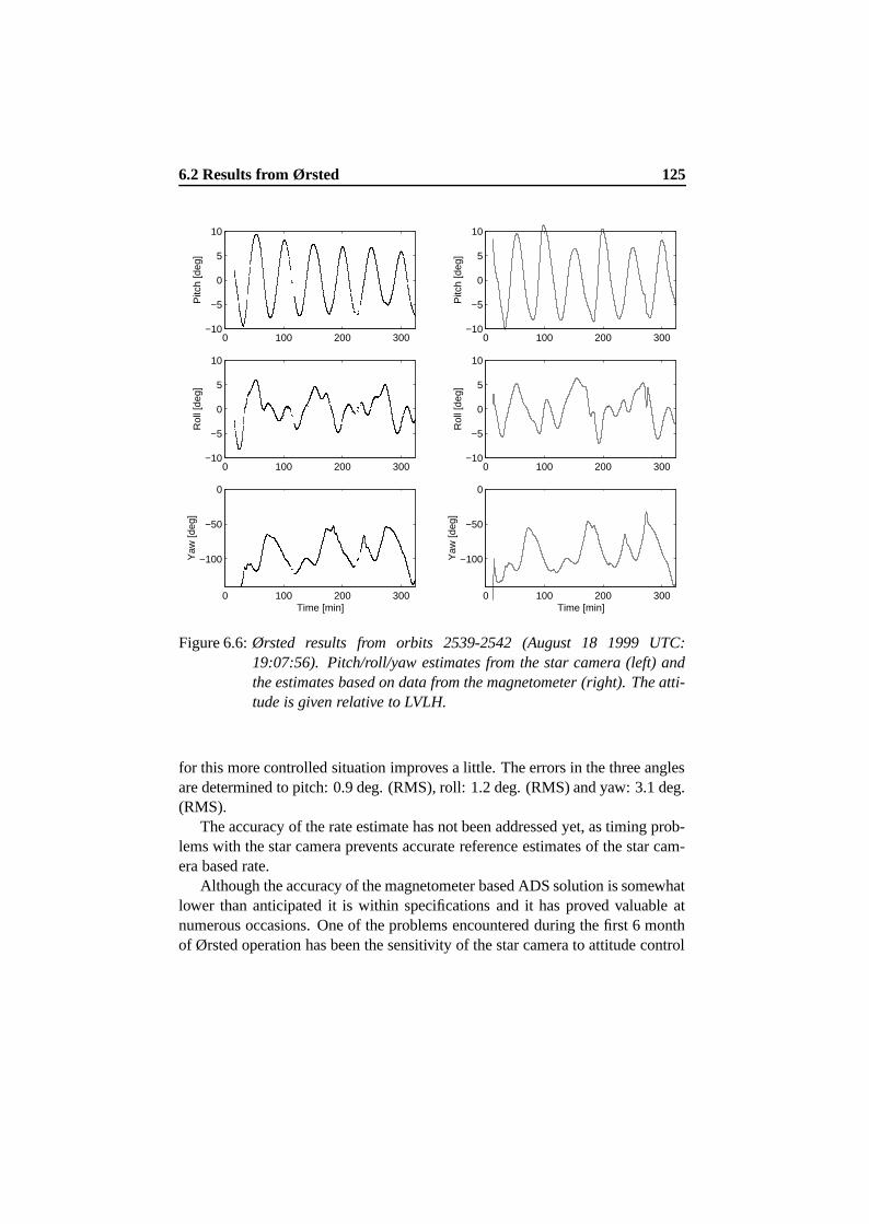
6.2 Results from Ørsted 125
0 100 200 300−10
−5
0
5
10
Pitc
h [d
eg]
0 100 200 300−10
−5
0
5
10
Rol
l [de
g]
0 100 200 300
−100
−50
0
Yaw
[deg
]
Time [min]
0 100 200 300−10
−5
0
5
10
Pitc
h [d
eg]
0 100 200 300−10
−5
0
5
10
Rol
l [de
g]
0 100 200 300
−100
−50
0
Yaw
[deg
]
Time [min]
Figure 6.6: Ørsted results from orbits 2539-2542 (August 18 1999 UTC:19:07:56). Pitch/roll/yaw estimates from the star camera (left) andthe estimates based on data from the magnetometer (right). The atti-tude is given relative to LVLH.
for this more controlled situation improves a little. The errors in the three anglesare determined to pitch: 0.9 deg. (RMS), roll: 1.2 deg. (RMS) and yaw: 3.1 deg.(RMS).
The accuracy of the rate estimate has not been addressed yet, as timing prob-lems with the star camera prevents accurate reference estimates of the star cam-era based rate.
Although the accuracy of the magnetometer based ADS solution is somewhatlower than anticipated it is within specifications and it has proved valuable atnumerous occasions. One of the problems encountered during the first 6 monthof Ørsted operation has been the sensitivity of the star camera to attitude control
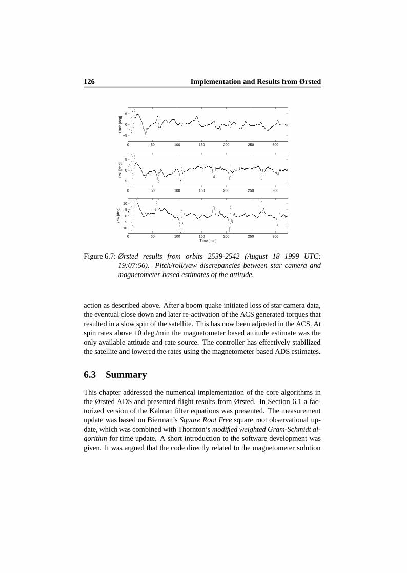
126 Implementation and Results from Ørsted
0 50 100 150 200 250 300
−5
0
5
Pitc
h [d
eg]
0 50 100 150 200 250 300
−5
0
5
Rol
l [de
g]
0 50 100 150 200 250 300
−10
−5
0
5
10
Yaw
[deg
]
Time [min]
Figure 6.7: Ørsted results from orbits 2539-2542 (August 18 1999 UTC:19:07:56). Pitch/roll/yaw discrepancies between star camera andmagnetometer based estimates of the attitude.
action as described above. After a boom quake initiated loss of star camera data,the eventual close down and later re-activation of the ACS generated torques thatresulted in a slow spin of the satellite. This has now been adjusted in the ACS. Atspin rates above 10 deg./min the magnetometer based attitude estimate was theonly available attitude and rate source. The controller has effectively stabilizedthe satellite and lowered the rates using the magnetometer based ADS estimates.
6.3 Summary
This chapter addressed the numerical implementation of the core algorithms inthe Ørsted ADS and presented flight results from Ørsted. In Section 6.1 a fac-torized version of the Kalman filter equations was presented. The measurementupdate was based on Bierman’s Square Root Free square root observational up-date, which was combined with Thornton’s modified weighted Gram-Schmidt al-gorithm for time update. A short introduction to the software development wasgiven. It was argued that the code directly related to the magnetometer solution

6.3 Summary 127
is responsible for less than 22% of ACS code.Finally Section 6.2 presented preliminary results from the Ørsted ADS. The
magnetometer based ADS was evaluated by comparison with available attitudeestimates from the star camera. The accuracy was found to be lower than ex-pected, but the hope is with adjustment of the filter noise parameters and moreaccurate analysis to get results that are more in line with the predicted results.The preliminary results from Ørsted do, however, meet the 2 deg. pitch/roll and4 deg. yaw (1 sigma) error specification.

Chapter 7
Freja Attitude Estimation
The second application described in this thesis is an attitude estimation algorithmfor the Freja satellite. The attitude is needed by the science mission to make off-line compensations of motion induced disturbances. At the present time onlycoarse, low rate attitude knowledge is available. A relatively high accuracy isrequired in order to fully utilize the science measurements.
This chapter presents the result of an effort to explore the use the extendedKalman filtering algorithms described in the previous chapters. The algorithmsare applied to magnetometer flight data and attitude data reconstructed. A num-ber of new issues had to be addressed in order to achieve the required accu-racy. The solution presented here provides attitude estimates also during eclipse,where no reliable attitude was previously available. The results in this chapterwere published in Bak (1998b), and Bak (1998a).
The chapter is divided into five sections and a summary. Section 7.1 givesthe motivation for addressing the Freja problem and outlines the previous attitudeestimation attempts and their limited usefulness. Section 7.2 address the requiredaccuracy and the implications for a potential estimator design. Section 7.3 dealswith the solution approach and Section 7.4 gives a brief description the filterdesign, batch interval selection and filter tuning. Finally, Section 7.5 discussesthe perspective for attitude reconstruction applied to the satellite Astrid-2.
7.1 Motivation and Related Work
The Freja spacecraft was launched on October 6, 1992, and delivered approxi-mately 200 megabytes of data each day until science observation ended in June
129
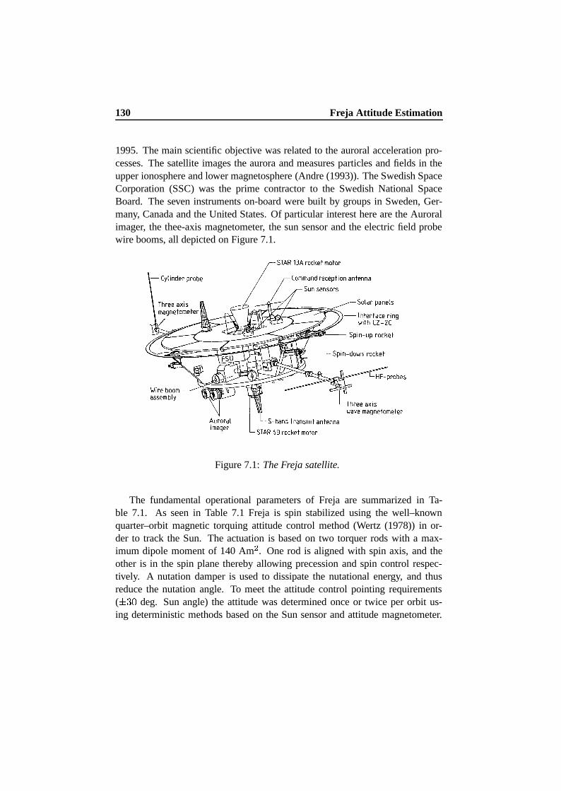
130 Freja Attitude Estimation
1995. The main scientific objective was related to the auroral acceleration pro-cesses. The satellite images the aurora and measures particles and fields in theupper ionosphere and lower magnetosphere (Andre (1993)). The Swedish SpaceCorporation (SSC) was the prime contractor to the Swedish National SpaceBoard. The seven instruments on-board were built by groups in Sweden, Ger-many, Canada and the United States. Of particular interest here are the Auroralimager, the thee-axis magnetometer, the sun sensor and the electric field probewire booms, all depicted on Figure 7.1.
Figure 7.1: The Freja satellite.
The fundamental operational parameters of Freja are summarized in Ta-ble 7.1. As seen in Table 7.1 Freja is spin stabilized using the well–knownquarter–orbit magnetic torquing attitude control method (Wertz (1978)) in or-der to track the Sun. The actuation is based on two torquer rods with a max-imum dipole moment of 140 Am  . One rod is aligned with spin axis, and theother is in the spin plane thereby allowing precession and spin control respec-tively. A nutation damper is used to dissipate the nutational energy, and thusreduce the nutation angle. To meet the attitude control pointing requirements( Ë � deg. Sun angle) the attitude was determined once or twice per orbit us-ing deterministic methods based on the Sun sensor and attitude magnetometer.
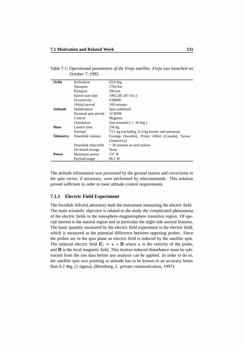
7.1 Motivation and Related Work 131
Table 7.1: Operational parameters of the Freja satellite. Freja was launched onOctober 7, 1992.
Orbit Inclination 63.0 deg.Apoapsis 1764 kmPeriapsis 596 kmEpoch start date 1992.281 (07 Oct.)Eccentricity 0.08000Orbital period 109 minutes
Attitude Stabilization Spin stabilizedNominal spin period 10 RPMControl MagneticOrientation Sun oriented (+/- 30 deg.)
Mass Launch time 256 kgPayload 73.1 kg (including 21.6 kg booms and antennas)
Telemetry Downlink stations Esrange (Sweden), Prince Albert (Canada), Syowa(Antarctica)
Downlink time/orbit < 30 minutes at each stationOn-board storage None
Power Maximum power 137 WPayload usage 66.1 W
The attitude information was processed by the ground station and corrections tothe spin vector, if necessary, were performed by telecommands. This solutionproved sufficient in order to meet attitude control requirements.
7.1.1 Electric Field Experiment
The Swedish Alfvén Laboratory built the instrument measuring the electric field.The main scientific objective is related to the study the complicated phenomenaof the electric fields in the ionosphere-magnetosphere transition region. Of spe-cial interest is the auroral region and in particular the night side auroral features.The basic quantity measured by the electric field experiment is the electric field,which is measured as the potential difference between opposing probes. Sincethe probes are in the spin plane an electric field is induced by the satellite spin.The induced electric field �l¡Q�D\ �v� where \ is the velocity of the probe,and � is the local magnetic field. This motion induced disturbance must be sub-tracted from the raw data before any analysis can be applied. In order to do so,the satellite spin axis pointing or attitude has to be known to an accuracy betterthan 0.2 deg. (1 sigma), (Blomberg, L. private communication, 1997).
132 Freja Attitude Estimation
The accuracy of the present single frame solution is unclear. More important,however, the single frame solution fails during eclipse when the Sun reference isnot available. This is a major difficulty as a number of interesting phenomena inthe polar ionosphere take place in the night-side auroral oval.
Determining the attitude based on interpolation of the single frame attitudesolution before and after eclipse has proved problematic. The passage of thespacecraft in and out of eclipse complicates the problem. The decrease in tem-perature during orbit night cause the coil booms to shrink, shortening the boomsradial distance to the spacecraft center of mass, thereby decreasing the momentsof inertia.
An alternative solution is therefore needed that allow the estimation of a com-plete attitude time history during the polar cap passage. One approach that hasbeen applied was based on the UV-imager. The ultra violet CCD camera waspointed towards the stars and a star identification algorithm combined with anattitude determination was applied. The results deviated significantly from atti-tude estimated for attitude control purposes. The UV-imager based attitude is,however, only available for six selected orbits.
7.1.2 A Magnetometer based Approach for Freja
Although the Freja satellite is fundamentally different from Ørsted, some of thesame attitude estimation methods may still be applied. As demonstrated in theprevious chapter, a single three axis magnetometer may provide us with valu-able information about the spacecraft attitude state also during eclipse. Usingthe measured magnetic field data in an attitude solution will attribute any longperiodic changes in the observed field to changes in the attitude of the spacecraft.As the main scientific interest is related to short periodic structures, the use ofthe same data for attitude estimation will not significantly affect the science mea-surements.
7.1.2.1 The Magnetic Field Experiment
Freja also flies a magnetic field experiment. The magnetometer is a triaxial corefluxgate sensor (Ballard and Hayes (1992) and Andre (1993)) mounted on a2 meter boom, seen on the left in Figure 7.1.
The fluxgate type instrument senses all three components of the magneticfield with range of ò 4&i ����� nT and provides a resolution of 2 nT. The magneticfield vector is sampled at 128 Hz. Data is already part of the post processing of
7.2 The Attitude Problem 133
the electric field measurements and thus available for attitude estimation.
A number of issues are new in the Freja problem compared to whatwas described in Chapter 5. The main challenge is the need for accuracy(0.2 deg. (1 sigma)) over the entire science observation interval. This accuracyrequirement changes some of the issues discussed in relation to the Ørsted designand a number of the assumptions have to be re-addressed.
7.2 The Attitude Problem
The Freja problem is to estimate the three-axis attitude time history
5¯lkt³
duringscience observation. The attitude quaternion parameterizes the transformationfrom inertial coordinates to spacecraft body coordinates. The basic input is thescience magnetometer measurement. As science data is investigated off-line inbatches, the attitude estimation may be treated as a smoothing problem. Theattitude estimate at a given instant can hence be based on data that fall bothbefore and after that time.
7.2.1 Magnetometer Calibration
Calibration of the magnetometer may possibly be carried out directly as part ofthe estimation process, but off-line parameter identification of sensor sensitivity,bias, orthogonality, misalignment may help simplify the estimator design signif-icantly. Moreover all these issues have previously been addressed in the as partof the magnetic field experiment (Luehr (1997)) and we could take advantage ofthese earlier results.
Magnetometers are inherently nonlinear devices and an accurate calibrationof the magnetometer is required to get to the specified accuracy (Freja 2 nT).The calibration converts the raw engineering units measured by the instrumentsinto field components in nT along three orthogonal Cartesian coordinate axes.The calibration may be carried out in a coil facility prior to launch. Stress dur-ing launch and operation in the space environment may, however, significantlychange the instrument transfer function, and an in-flight calibration is thereforenormally required.
Luehr (1997) has showed that a complex non-linear in-flight calibration ofthe magnetometer is necessary in order to get to the 2 nT noise level. Thisnoise level is well below the 0.2 deg. accuracy requirement and a simple linear
134 Freja Attitude Estimation
approach has been taken. The result is a calibration according to� �F� ¯���r £w� ³ (7.1)
where � is the measured field in nT, q is theË � Ë orthogonality and sensitivity
correction matrix,���
is the raw measurement vector in engineering units, and¿ is a bias vector in engineering units. All parameters are estimate based on aleast square fitting.
The magnetic field vector measurement is made in the magnetometer assem-bly coordinate system, where the z-axis was designed to be parallel to the satel-lite spin axis and the other two axes lie in the spin plane. It was found, however,that a correction on the order of a few tenths of a deg. was necessary for thealignment of the instrument.
This correction was implemented as follows: First, the > - and 7 - axis mea-surements were fitted with a sinusoidal wave with a shifted baseline and alinearly-varying envelop. The satellite spin period is determined from the os-cillation period of these two components, whereas the cross-component phaselag gives the information about the angle between the > and 7 axes. The ratiobetween the > / 7 -component offset to the ; -component measurement provides aninclination of the ; -axis from the satellite spin axis.
Based on those results the measured magnetic field vector is rotated from theinstrument assembly frame to the spacecraft body frame.
7.2.2 Reference Model Accuracy
While the calibration is carried out off-line and thereby simplifying the estimatordesign, the accuracy of the reference model has to be addressed directly in theestimator design.
One of the science objectives of Freja and of the electric field experimentin particular is the investigation of field aligned currents that are present inthe auroral region. The field aligned currents results in magnetic perturbationsperpendicular to the main field. As the Freja orbit goes through the auroraloval these perturbations may significantly vary in magnitude from fractions ofa nT to thousands of nT Langel (1987). When using the magnetometer data inan attitude solution, periods with large perturbations must be avoided as theseperturbations would otherwise influence the attitude estimates. As it will beshown later in this chapter, perturbations in the order of 300 nT may occur,which if attributed to attitude changes, would result in attitude errors as largeas ���W� � ��� ¯²Ë ���#_ Ë �ai ����� ³ ���ai ò deg..

7.3 Estimator Design 135
In order to avoid this contamination of the attitude estimation, these pertur-bations to the field must be detected by the attitude determination system andthe measurements must be rejected or corrected before being applied in the atti-tude estimator. When measurements are rejected the propagation will have to bebased on an accurate dynamic model between measurement updates as no gyrosare available.
7.2.3 Accuracy of Dynamic Model
The need for 0.2 deg. accuracy combined with possible propagation over con-taminated data gaps emphasizes the need for an accurate dynamic model. Pas-sage of the spacecraft in and out of eclipse further complicates the problem. Pre-sumably the temperature change cause the coil booms to shrink when they cooldown during orbit night shortening the booms radial distance to the spacecraftcenter of mass, thereby decreasing the moments of inertia. An simple propaga-tion of the spin frequency through the day/night transition will hence not work.Assuming zero torques on the spacecraft, the angular momentum is known tobe constant during such a transition, and any change in spin frequency may bereferred to the a change in the moments of inertia about the spin axis.
An additional effect to shrinking of the booms, is that heat dissipation in thebooms due to bending will cause the system to lose energy. This drift is, assumednegligible during the relative short time intervals considered here.
The inherent magnetic residual in the spacecraft was minimized during de-sign, to reduce disturbances on the measurements. Magnetically induced torquesare therefore assumed negligible.
7.3 Estimator Design
The attitude reconstruction problem has been solved using an estimator similarto the one developed for Ørsted. The estimator maintains an accurate dynamicmodel of the spacecraft, which is used to propagate the attitude and angular ve-locity estimates through the data gap. The dynamic model propagation is basedon estimates of the on-orbit spacecraft inertias. The thermally induced changesin the moments of inertia are estimated through a parameter in the filter, therebyconserving angular momentum. Updates of the model are performed wheneverreliable magnetometer data are available. The data gaps are identified using thea residual monitoring algorithm described below.
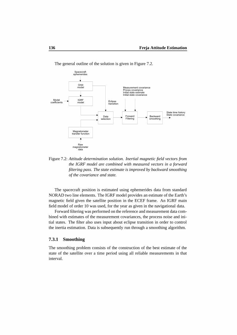
136 Freja Attitude Estimation
The general outline of the solution is given in Figure 7.2.
Figure 7.2: Attitude determination solution. Inertial magnetic field vectors fromthe IGRF model are combined with measured vectors in a forwardfiltering pass. The state estimate is improved by backward smoothingof the covariance and state.
The spacecraft position is estimated using ephemerides data from standardNORAD two line elements. The IGRF model provides an estimate of the Earth’smagnetic field given the satellite position in the ECEF frame. An IGRF mainfield model of order 10 was used, for the year as given in the navigational data.
Forward filtering was performed on the reference and measurement data com-bined with estimates of the measurement covariances, the process noise and ini-tial states. The filter also uses input about eclipse transition in order to controlthe inertia estimation. Data is subsequently run through a smoothing algorithm.
7.3.1 Smoothing
The smoothing problem consists of the construction of the best estimate of thestate of the satellite over a time period using all reliable measurements in thatinterval.
7.3 Estimator Design 137
Let an estimate of the initial state atk * be given and denote it by
�¤ * . Theerror in this initial estimate is assumed to be Gaussian with zero mean and co-variance ¯°* . The filtered estimate at time
k ¨ is designated by ¤��¨ . Given is a setof discrete measurements
ª £ µ Ä � · Ö i i i�� ¬ , we process the measurements se-quentially forward in time and produce the sequence
ª �¤ � Ö ¯ � ÖWÄ � · Ö i�i�i Ö � ¬ .The smoothing algorithm produces the sequence
ª �¤�� Ö ¯ � ÖWÄ �F� Ö i�i�i Ö · ¬ , withthe initial smoothed estimate at � being provided by the filtered estimate at � .
Forward Filtering Pass The magnetic field observations are processed in aforward pass using the Kalman filter described in Chapter 4.
The thermally induced variations in moments of inertia are known to be cor-related with the day/night and night/day transitions. In order to allow the filterto track these inertia changes, the noise model is synchronized with the eclipsetransitions. After an eclipse transition, the inertia covariance is reset to its origi-nal value and a new constant bias is estimated.
Backward Smoothing The smoothing algorithm is based on the Rauch-Tung-Striebel (R-T-S) fixed interval smoothing algorithm (Rauch et al. (1965)).
During the forward filtering the intermediate results�¤ ¥ , ¯ ¥ , �¤ ¥ Y » ,¯ ¥ Y » and Õ Õ ¯lk Ö8k Y » ³ are stored at each time
k . The smoothing pass runsbackward in time from the time
k"�of the last measurement, computing the
smoothed state estimate from the intermediate results. The smoothed state esti-mate and its covariance are initialized with the a posteriori values�¤ I� � �¤ � ¥ � (7.2)¯ I� � ¯ � ¥ � (7.3)
The smoothed estimates are then computed recursively usingº � ¯ ¥ Õ Õ ¯lk Ö8k Y » ³ ¯ Y » b »W¥ (7.4)�¤ I � �¤ ¥ £<º » ¤ I b » � �¤ b »W¥ ½ (7.5)
7.3.2 Process Model
The filter error state vector is composed of the vector part of the inertial to bodyattitude quaternions and the three angular rate corrections. To account for ther-mally induced perturbation to the maximum moment of inertia, a perturbation tothe spin axis moment of inertia is included in the state vector
138 Freja Attitude Estimation
The result is a 7 dimensional perturbational state vectorm ¤�� ��ó m±4�ÕHm±wûÕ õ Î�÷ Õ (7.6)
where w are the inertial body rates represented in the body frame. The fullquaternion 4 parameterize the rotation from inertial to the body frame.
õ Î is themaximum (spin axis) moment of inertia. The perturbation to the maximum prin-cipal moment of inertia is used to model the thermally induced inertia variations.Such a model automatically conserve angular momentum and it was found to berequired in order to propagate the attitude and rate estimates accurately throughdata gaps.
The vehicle attitude process model follows the equations derived in Chapter 3with small modifications due to the inclusion of the extra inertia state and the factthat the Freja attitude is given relative to inertial space.
The variableõ Î is estimated using a bias model that is a random constant
generated as the output of an integrator with no input, thus|| k õ Î ¯lkt³ �Q� (7.7)
The initial condition is specified by the meanõ Î * and the variance cV¡ * . The
selection of this kind of model is based on the assumption that the inertia isunknown but constant over the interval under investigation. The filter will useinitial data to estimate the constant and eventually disregard all later measure-ments. After an eclipse transition, the filter is reset, and the filter will use thenew measurements to converge to a new constant value, which hopefully repre-sents the modified moment of inertia. The measurement formulation follows theØrsted measurement model.
The initial full state estimates are derived from the coarse attitude data avail-able in the present attitude history files, and is set equal to4 * � ø �e�ai[� ò � 2 Ö �ai � h M Ë�Ö �e�ai^M�M Ë 2 Ö �ai[��� Ë�Ë úÑÕ (7.8)w * � ø � Ö � Ö · i � h ·�· ú Õ (7.9)�^*Ç�
�� 2 4&i Ë 2 � � �� h · i Ë�Ë 4 �� � · 4 2 i ò M 2�
(7.10)
The measurement noise model has been addressed previously in Sec-tion 5.3.2.1 while the process noise intensity were found empirically to obtain
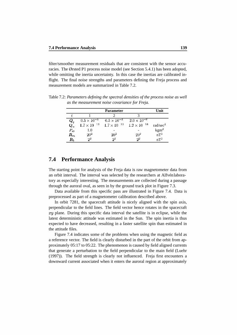
7.4 Performance Analysis 139
filter/smoother measurement residuals that are consistent with the sensor accu-racies. The Ørsted P1 process noise model (see Section 5.4.1) has been adopted,while omitting the inertia uncertainty. In this case the inertias are calibrated in-flight. The final noise strengths and parameters defining the Freja process andmeasurement models are summarized in Table 7.2.
Table 7.2: Parameters defining the spectral densities of the process noise as wellas the measurement noise covariance for Freja.
Parameter UnitO1 2 3_ � )P !��(&*) �SU )pP[!ï�©&�) �VU W P )ï�(&*) �SU_�� &TP Y �(&*) ���Z &TP Y �(&*) ���B &TP W �(&*) ���8� rad/sec � a5� 1.0 - - kgm 0 n W ) W ) W ) nT 0 � W W W nT
7.4 Performance Analysis
The starting point for analysis of the Freja data is raw magnetometer data froman orbit interval. The interval was selected by the researchers at Alfvén labora-tory as especially interesting. The measurements are collected during a passagethrough the auroral oval, as seen in by the ground track plot in Figure 7.3.
Data available from this specific pass are illustrated in Figure 7.4. Data ispreprocessed as part of a magnetometer calibration described above.
In orbit 7281, the spacecraft attitude is nicely aligned with the spin axis,perpendicular to the field lines. The field vector hence rotates in the spacecraft> 7 plane. During this specific data interval the satellite is in eclipse, while thelatest deterministic attitude was estimated in the Sun. The spin inertia is thusexpected to have decreased, resulting in a faster satellite spin than estimated inthe attitude files.
Figure 7.4 indicates some of the problems when using the magnetic field asa reference vector. The field is clearly disturbed in the part of the orbit from ap-proximately 05:17 to 05:22. The phenomenon is caused by field aligned currentsthat generate a perturbation to the field perpendicular to the main field (Luehr(1997)). The field strength is clearly not influenced. Freja first encounters adownward current associated when it enters the auroral region at approximately
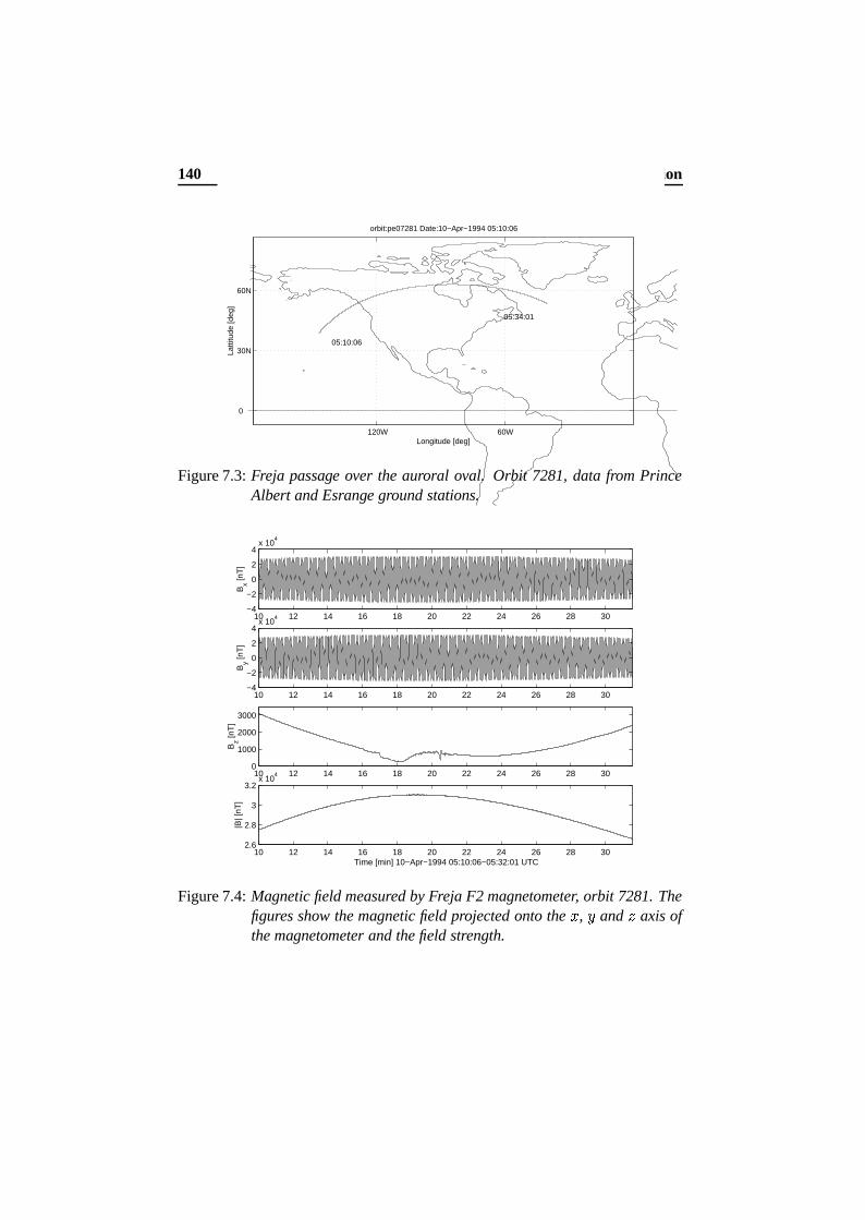
140 Freja Attitude Estimation
120W 60W
0
30N
60N
Longitude [deg]
Latti
tude
[deg
]orbit:pe07281 Date:10−Apr−1994 05:10:06
05:10:06
05:34:01
Figure 7.3: Freja passage over the auroral oval. Orbit 7281, data from PrinceAlbert and Esrange ground stations.
10 12 14 16 18 20 22 24 26 28 30−4
−2
0
2
4x 10
4
Bx [n
T]
10 12 14 16 18 20 22 24 26 28 30−4
−2
0
2
4x 10
4
By [n
T]
10 12 14 16 18 20 22 24 26 28 300
1000
2000
3000
Bz [n
T]
10 12 14 16 18 20 22 24 26 28 302.6
2.8
3
3.2x 10
4
|B| [
nT]
Time [min] 10−Apr−1994 05:10:06−05:32:01 UTC
Figure 7.4: Magnetic field measured by Freja F2 magnetometer, orbit 7281. Thefigures show the magnetic field projected onto the > , 7 and ; axis ofthe magnetometer and the field strength.

7.4 Performance Analysis 141
05:17. At approximately 05:19 it encounters a discontinuity, at which the fieldsignature changed rapidly. The discontinuity occurs within a region of upwardcurrent. Finally Freja leaves the auroral oval at approximately 05:21.
Applying the filter directly the measured field with an error of 300 nT resultsin an error of approximately atan
¯²Ë ���#_ Ë ������� ³ ���ai ò deg.. The problem is solvedselecting a batch interval outside this region. The result is a data gap, where thestate estimation will have to be based on integration of the equations of motionof the spacecraft.
Assuming that field aligned currents cause the phenomena seen in Figure 7.4the disturbance to the main field is mainly perpendicular to the spin axis. In thecase in Figure 7.4 this would leave the > and 7 components of the measurementsinvariant, and they could be used in the filter. The attitude is, however, not alwaysas nicely aligned as in Figure 7.4 and the estimator is hence designed with nomeasurement updates in the disturbed region.
It is evident that in order to automate the estimation process and at the sametime get the required accuracy, disturbance detection is necessary. A simple testbased on the log-likelihood ratio is proposed and applied in the following.
7.4.1 Attitude Reconstruction Results
The filter/smoother output includes several types of data that illustrate its per-formance. The measurement residual time histories indicate the filter/smoothersability to fit the data. The attitude time histories illustrate the general state esti-mate.
Figure 7.5 shows the estimated and measured field measurements for the7281 orbit.
Measurement Residual Time Histories The measurement residual vector is£ �j� ¯ �¤ I ¥ Ö8k ³ . The result should be a noise sequences with a RMS valuesless than or equal to the diagonal elements of the measurement noise covariance,² . If the process noise intensity were very small, then the measurement resid-ual sequences would be almost white noise with RMS values approaching thediagonal elements of ² .
Figure 7.6 shows the estimated F2 measurement residual time history.The attitude is propagated from 05:16–05:24. The measurement residuals
outside the data gap has RMS values are around 20 nT in the > and 7 compo-nents, which is in good agreement with the observation noise. A 20 nT error inthe field components approximately correspond to an angular error of 0.04 deg.
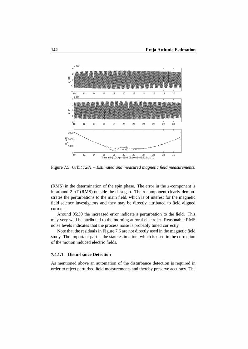
142 Freja Attitude Estimation
10 12 14 16 18 20 22 24 26 28 30−4
−2
0
2
4x 10
4
Bx [n
T]
10 12 14 16 18 20 22 24 26 28 30−4
−2
0
2
4x 10
4
By [n
T]
10 12 14 16 18 20 22 24 26 28 300
1000
2000
3000
Bz [n
T]
Time [min] 10−Apr−1994 05:10:06−05:32:01 UTC
Figure 7.5: Orbit 7281 – Estimated and measured magnetic field measurements.
(RMS) in the determination of the spin phase. The error in the ; -component isin around 2 nT (RMS) outside the data gap. The ; component clearly demon-strates the perturbations to the main field, which is of interest for the magneticfield science investigators and they may be directly attributed to field alignedcurrents.
Around 05:30 the increased error indicate a perturbation to the field. Thismay very well be attributed to the morning auroral electrojet. Reasonable RMSnoise levels indicates that the process noise is probably tuned correctly.
Note that the residuals in Figure 7.6 are not directly used in the magnetic fieldstudy. The important part is the state estimation, which is used in the correctionof the motion induced electric fields.
7.4.1.1 Disturbance Detection
As mentioned above an automation of the disturbance detection is required inorder to reject perturbed field measurements and thereby preserve accuracy. The
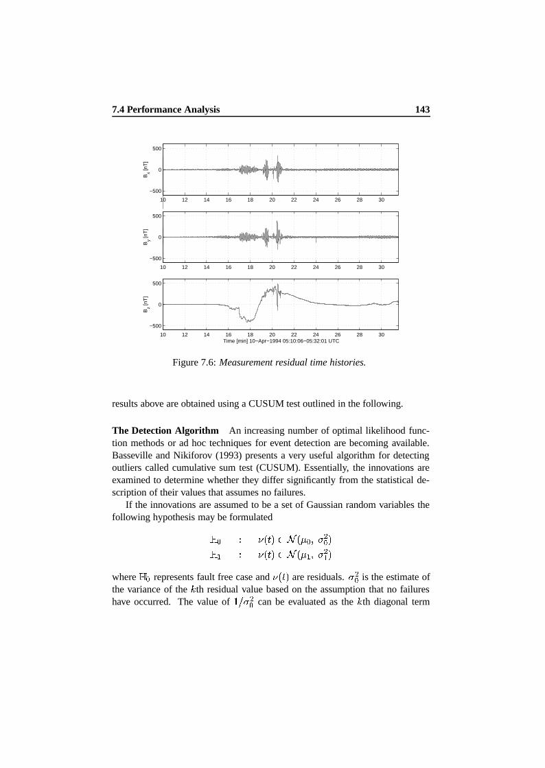
7.4 Performance Analysis 143
10 12 14 16 18 20 22 24 26 28 30
−500
0
500B
x [nT
]
10 12 14 16 18 20 22 24 26 28 30
−500
0
500
By [n
T]
10 12 14 16 18 20 22 24 26 28 30
−500
0
500
Bz [n
T]
Time [min] 10−Apr−1994 05:10:06−05:32:01 UTC
Figure 7.6: Measurement residual time histories.
results above are obtained using a CUSUM test outlined in the following.
The Detection Algorithm An increasing number of optimal likelihood func-tion methods or ad hoc techniques for event detection are becoming available.Basseville and Nikiforov (1993) presents a very useful algorithm for detectingoutliers called cumulative sum test (CUSUM). Essentially, the innovations areexamined to determine whether they differ significantly from the statistical de-scription of their values that assumes no failures.
If the innovations are assumed to be a set of Gaussian random variables thefollowing hypothesis may be formulated2 * Ü � ¯lk�³oÆK�Ó¯l� * Ö 1 Â* ³2P» Ü � ¯lk�³oÆK�Ó¯l� » Ö 1b» ³where 2�* represents fault free case and � ¯lk�³ are residuals. 1 Â* is the estimate ofthe variance of the
Äth residual value based on the assumption that no failures
have occurred. The value of · _�1 Â* can be evaluated as theÄ
th diagonal term
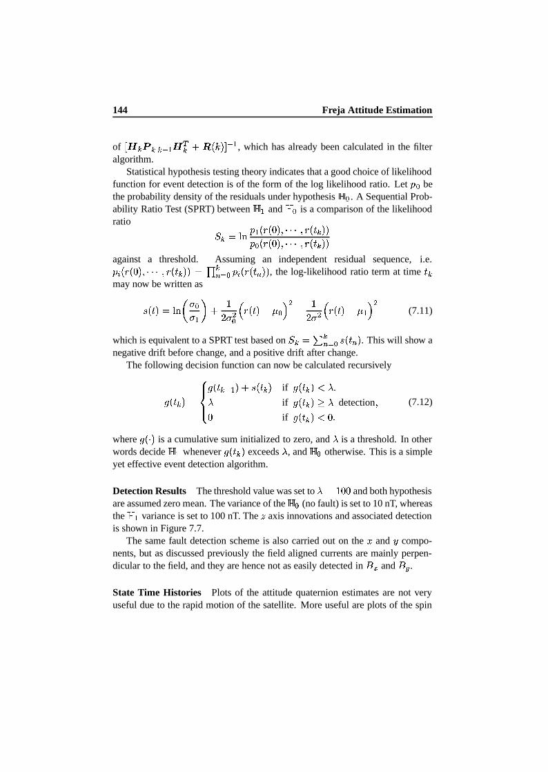
144 Freja Attitude Estimation
of ø¶Ã ¯ ¥ Y » Ã Õ £Q² ¯´Ä�³ ú Y » , which has already been calculated in the filteralgorithm.
Statistical hypothesis testing theory indicates that a good choice of likelihoodfunction for event detection is of the form of the log likelihood ratio. Let Ù1* bethe probability density of the residuals under hypothesis 2 * . A Sequential Prob-ability Ratio Test (SPRT) between 2�» and 2d* is a comparison of the likelihoodratio È � x � ÙD» ¯ � ¯ � ³*Ö ����� Ö � ¯lk ³t³Ù�* ¯ � ¯ � ³*Ö ����� Ö � ¯lk ³t³against a threshold. Assuming an independent residual sequence, i.e.Ù�¡ ¯ � ¯ � ³*Ö ����� Ö � ¯lk ³t³ ��� ¸ º+* Ù�¡ ¯ � ¯lk ¸ ³t³ , the log-likelihood ratio term at time
k may now be written asE ¯lk�³ � x � o 1 *1b» q £ ·��1 Â*�� � ¯lk�³ � � *��  � ·
��1 »�� � ¯lk�³ � � »��  (7.11)
which is equivalent to a SPRT test based onÈ �N ¸ º+* E ¯lk ¸ ³ . This will show a
negative drift before change, and a positive drift after change.The following decision function can now be calculated recursively
¡ ¯lk ³ � ¢£¤ £¥¡ ¯lk Y » ³ £¦E ¯lk ³ if ¡ ¯lk ³NШ§bÖ§
if ¡ ¯lk ³ � §detection
Ö� if ¡ ¯lk ³NÐ �ai (7.12)
where ¡ ¯ � ³ is a cumulative sum initialized to zero, and§
is a threshold. In otherwords decide 2�» whenever ¡ ¯lk ³ exceeds
§, and 2d* otherwise. This is a simple
yet effective event detection algorithm.
Detection Results The threshold value was set to§ � · ��� and both hypothesis
are assumed zero mean. The variance of the 2 * (no fault) is set to 10 nT, whereasthe 2 » variance is set to 100 nT. The ; axis innovations and associated detectionis shown in Figure 7.7.
The same fault detection scheme is also carried out on the > and 7 compo-nents, but as discussed previously the field aligned currents are mainly perpen-dicular to the field, and they are hence not as easily detected in © ¾ and ©]ª .State Time Histories Plots of the attitude quaternion estimates are not veryuseful due to the rapid motion of the satellite. More useful are plots of the spin
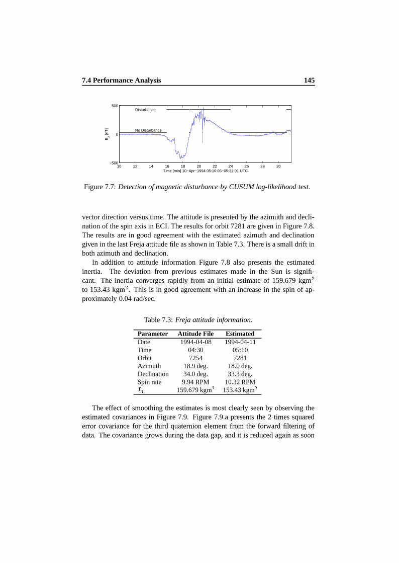
7.4 Performance Analysis 145
10 12 14 16 18 20 22 24 26 28 30−500
0
500
Time [min] 10−Apr−1994 05:10:06−05:32:01 UTC
Bz [n
T]
Disturbance
No Disturbance
Figure 7.7: Detection of magnetic disturbance by CUSUM log-likelihood test.
vector direction versus time. The attitude is presented by the azimuth and decli-nation of the spin axis in ECI. The results for orbit 7281 are given in Figure 7.8.The results are in good agreement with the estimated azimuth and declinationgiven in the last Freja attitude file as shown in Table 7.3. There is a small drift inboth azimuth and declination.
In addition to attitude information Figure 7.8 also presents the estimatedinertia. The deviation from previous estimates made in the Sun is signifi-cant. The inertia converges rapidly from an initial estimate of 159.679 kgm Âto 153.43 kgm  . This is in good agreement with an increase in the spin of ap-proximately 0.04 rad/sec.
Table 7.3: Freja attitude information.
Parameter Attitude File EstimatedDate 1994-04-08 1994-04-11Time 04:30 05:10Orbit 7254 7281Azimuth 18.9 deg. 18.0 deg.Declination 34.0 deg. 33.3 deg.Spin rate 9.94 RPM 10.32 RPM« 159.679 kgm 153.43 kgm
The effect of smoothing the estimates is most clearly seen by observing theestimated covariances in Figure 7.9. Figure 7.9.a presents the 2 times squarederror covariance for the third quaternion element from the forward filtering ofdata. The covariance grows during the data gap, and it is reduced again as soon
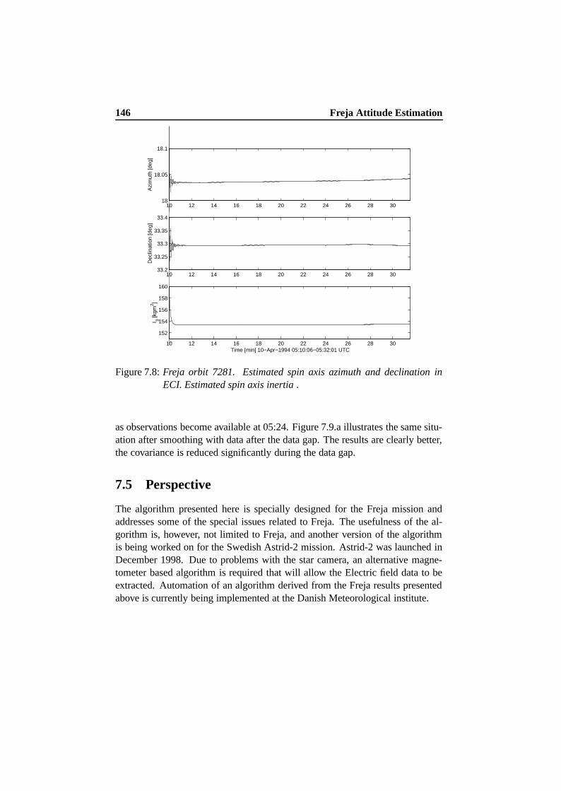
146 Freja Attitude Estimation
10 12 14 16 18 20 22 24 26 28 3018
18.05
18.1A
zim
uth
[deg
]
10 12 14 16 18 20 22 24 26 28 3033.2
33.25
33.3
33.35
33.4
Dec
linat
ion
[deg
]
10 12 14 16 18 20 22 24 26 28 30
152
154
156
158
160
I 3 [kgm
2 ]
Time [min] 10−Apr−1994 05:10:06−05:32:01 UTC
Figure 7.8: Freja orbit 7281. Estimated spin axis azimuth and declination inECI. Estimated spin axis inertia .
as observations become available at 05:24. Figure 7.9.a illustrates the same situ-ation after smoothing with data after the data gap. The results are clearly better,the covariance is reduced significantly during the data gap.
7.5 Perspective
The algorithm presented here is specially designed for the Freja mission andaddresses some of the special issues related to Freja. The usefulness of the al-gorithm is, however, not limited to Freja, and another version of the algorithmis being worked on for the Swedish Astrid-2 mission. Astrid-2 was launched inDecember 1998. Due to problems with the star camera, an alternative magne-tometer based algorithm is required that will allow the Electric field data to beextracted. Automation of an algorithm derived from the Freja results presentedabove is currently being implemented at the Danish Meteorological institute.
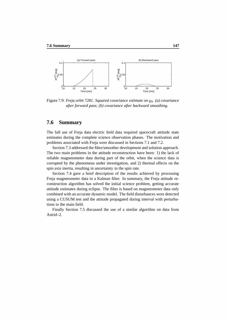
7.6 Summary 147
10 15 20 25 300
0.05
0.1
Time [min]
2P1/
2q3
[deg
]
(a) Forward pass
10 15 20 25 300
0.05
0.1
Time [min]
2P1/
2q3
[deg
]
(b) Backward pass
Figure 7.9: Freja orbit 7281. Squared covariance estimate on 3 Î . (a) covarianceafter forward pass; (b) covariance after backward smoothing.
7.6 Summary
The full use of Freja data electric field data required spacecraft attitude stateestimates during the complete science observation phases. The motivation andproblems associated with Freja were discussed in Sections 7.1 and 7.2.
Section 7.3 addressed the filter/smoother development and solution approach.The two main problems in the attitude reconstruction have been: 1) the lack ofreliable magnetometer data during part of the orbit, when the science data iscorrupted by the phenomena under investigation, and 2) thermal effects on thespin axis inertia, resulting in uncertainty in the spin rate.
Section 7.4 gave a brief description of the results achieved by processingFreja magnetometer data in a Kalman filter. In summary, the Freja attitude re-construction algorithm has solved the initial science problem, getting accurateattitude estimates during eclipse. The filter is based on magnetometer data onlycombined with an accurate dynamic model. The field disturbances were detectedusing a CUSUM test and the attitude propagated during interval with perturba-tions to the main field.
Finally Section 7.5 discussed the use of a similar algorithm on data fromAstrid–2.

Chapter 8
Conclusion andRecommendations
This thesis considered a number of aspects related to spacecraft attitude determi-nation. The problem of estimating the attitude based on magnetometer measure-ments only was studied in detail. This chapter summarizes the work presented inthis thesis. The main results are review and directions for further investigationsare identified.
8.1 Conclusion
Theory and application was combined in this thesis. First some basic theoreticalproblems were addressed and at the end two real flight cases were investigatedin detail. Results demonstrate the usefulness of magnetometer based solutionsto attitude estimation, as a backup on small satellites demanding coarse attitudeknowledge, or as a batch-processing reconstruction algorithm used in connectionwith a science mission.
The following conclusions are drawn on the accomplishments and contribu-tions of this thesis:
– A general discussion of attitude representation was presented and the ad-vantages of using a four component quaternion as rotation group specifiedwas outlined. The quaternion provides a globally nonsingular two-to-onemapping of the rotation group. A unit norm constraint limits the numberof independent parameters to one. An exponential series expansion of the
149
150 Conclusion and Recommendations
quaternion was presented, which may easily be truncated in linearization.It was argued that the series may be interpreted as a series of �(�¦� skewsymmetric matrices.
– An introduction to nonlinear attitude estimation based on Kalman filter-ing was given. It was demonstrated how temporal fusion of measurementsmakes full three-axis attitude determination possible with only one refer-ence sensor.
– Consistency of the estimator in the presence of modeling errors was inves-tigated. Given knowledge of the true system, limits on the noise statisticswere established that prevents inconsistency of the estimator.
– The problems of preserving normalization of the quaternion and covari-ance singularity were demonstrated by use of the exponential quater-nion series. The covariance singularity is numerically problematic, anda quaternion error approach was therefore taken that avoids the singular-ity by only estimating the three independent parameters in a first orderapproximation of the exponential series.
– An ADS design, where the magnetometer attitude estimate was used asa backup algorithm was presented. The result is a fault tolerant system,which enhance the autonomy of the Ørsted small satellite. Intense simula-tions based on a truth model has been carried out demonstrating the abilityof the system to estimate attitude and rates with the required accuracy.
– Flight results from Ørsted demonstrates how a single magnetometer mayprovide us with valuable information about the state of the spacecraft. Theuse of a simple magnetometer combined with an attitude estimator hascomplemented the more sophisticated star camera and provided estimatesof rate and attitude when the star camera constraints were violated. Dueto boom oscillations and other problems this has frequently been the caseover the first months of operation.
– Finally the Freja problem was addressed. The solution approach was out-lined and the results evaluated against available reference data. The result-ing estimator solved the problem of estimating the attitude during eclipseand data gaps. The filter state was augmented with an inertia state in orderto facilitate accurate propagation during periods with perturbed field data.

8.2 Recommendations 151
Perturbations to the field were automatically detected by use of a statisti-cal test. The accuracy of the solution solved the initial problem posed andenabled the compensation of motion induced disturbances on the electricscience field measurements, thereby enhancing the Freja science mission.
8.2 Recommendations
The following topics are not covered in this work but it is believed that futureinvestigations could be beneficial:
– With the advent of modern microprocessors, it has become increasinglypossible to produce smart sensors in which the state estimation process ismoved inside the sensor box. A typical example is the user segment of theGPS in which the receiver and navigation software are usually integratedinto a single processor. The implementation of an attitude estimator withthe magnetometer could be an interesting new application of the magne-tometer based attitude determination.
– The Ørsted data give us valuable new data and a high accuracy reference,which will allow additional studies of magnetometer based solutions onreal flight data. Problems with the Ørsted data are being addressed but afew problems related to the star camera timing and the boom oscillationsremain open.
– The areas of nonlinear observers and differential geometry has in recentyears received a lot of research interest. The results in these areas couldpossibly be transferred to the attitude estimation problem, yielding solu-tions (quaternions) that evolved on the
ÈoÎmanifold and thereby avoid the
normalization problem entirely.

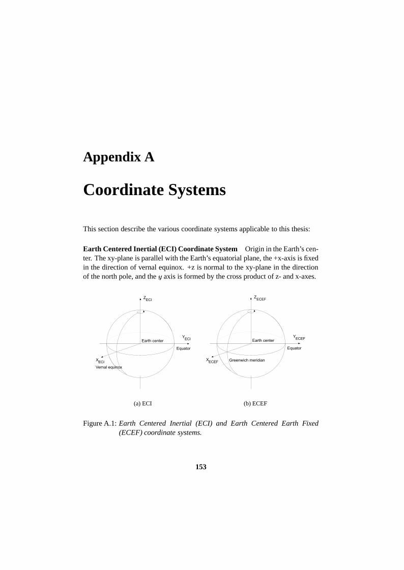
Appendix A
Coordinate Systems
This section describe the various coordinate systems applicable to this thesis:
Earth Centered Inertial (ECI) Coordinate System Origin in the Earth’s cen-ter. The xy-plane is parallel with the Earth’s equatorial plane, the +x-axis is fixedin the direction of vernal equinox. +z is normal to the xy-plane in the directionof the north pole, and the 7 axis is formed by the cross product of z- and x-axes.
(a) ECI (b) ECEF
Figure A.1: Earth Centered Inertial (ECI) and Earth Centered Earth Fixed(ECEF) coordinate systems.
153

154 Coordinate Systems
Spacecraft Body (SCB) Coordinate System Origin is defined in the space-craft structure and the frame is fixed to the spacecraft. The > 7 plane is definedby the interface plane where the satellite attaches to the launcher. The ; axis isnormal to the > 7 plane with the +z axis in the direction of the Ørsted boom, orthe “boresight” of the solar array in the Freja case. The Ørsted 7 axis is per-pendicular to the long side of the main body, while the Freja 7 axis is along themagnetometer booms with + 7 defined in the direction of the F2 magnetometer.The > axis completes the orthogonal coordinate system. The Ørsted SCB systemis given in Figure A.2(a) and the Freja SCB system in Figure A.2(b)
(a) Ørsted SCB (b) Freja SCB
Figure A.2: Ørsted and Freja SCB coordinate systems.
Principal (PCS) Coordinate System Origin is in the center of mass of thespacecraft. The axes are defined by the principal axes of the spacecraft withthe ; axis aligned with the spin axis of the spacecraft. The > and 7 axes areperpendicular to the ; axis. The rotation from SCB to P is implicit in this thesis.
Earth-Centered-Earth-Fixed (ECEF) Coordinate System Origin is at thecenter of mass of the Earth. The xy-plane coincide with the Earth’s equatorialplane, the +x-axis is fixed by the Greenwich Prime Meridian (GPM). +z is nor-mal to the xy-plane in the direction of the north pole, and the 7 axis is formedby the cross product of z- and x-axes, i.e. the 7 axis points 90 deg. to the east of

155
GPM.
Figure A.3: Local Vertical Local Horizontal coordinate system.
Local-Vertical-Local-Horizontal (LVLH) Coordinate System Origin is atthe center of mass of the spacecraft. The + ; axis (local vertical) is parallel to theradius vector, negative from the spacecraft center of mass to the center of Earth.The + > axis is pointed in the direction of the angular momentum vector (perpen-dicular to orbit plane). The 7 axis (local horizontal) completes the orthogonalcoordinate system. The + 7 lies in the orbit plane in the direction of the negativevelocity vector (only identical to the velocity vector for perfectly circular orbits).Note that this definition of LVLH deviates from traditional definitions.


Appendix B
Satellite and SpaceEnvironmental Models
B.1 Atmospheric Density Model
The Mass-Spectrometer-Incoherent-Scatter (MSIS-86) model describes the neu-tral temperature and densities in the upper atmosphere (above about 100 km). Itis used to model the large periodic changes in the atmospheric density. MSIS-86model an empirical model based on the extensive data compilation and analysiswork of Hedin (1987) and his colleagues.
B.2 Orbit Propagation Models
General perturbations element sets generated by NORAD are used to predictposition and velocity of the satellites. To do this one must be careful to use aprediction method which is compatible with the way in which the elements weregenerated.
Only ideal orbits describe true ellipses and have constant orbital elements.Real orbits experience both periodic and secular effects in their elements. Be-cause of this, there are various ways of describing orbital elements. One wayis to use osculating or instantaneous orbital elements, that is, the instantaneousvalues of each element at the specified epoch. The other is to use mean orbitalelements.
NORAD maintains general perturbation element sets (Two Line Elements(TLE’s) on all resident space objects. These element sets are periodically refined
157
158 Satellite and Space Environmental Models
so as to maintain a reasonable prediction capability on all space objects. In turn,these element sets are provided to users. The NORAD element sets are meanelements obtained by removing periodic variations in a particular way. In orderto obtain good predictions, these periodic variations must be reconstructed in thesame way they were removed by NORAD. Hence, inputting NORAD elementsets into a different model (even though the model may be more accurate or evena numerical integrator) will result in degraded predictions. The NORAD elementsets must be used with one of the models described in this report in order to retainmaximum prediction accuracy.
The Special General Perturbation (SGP4) model generate predictions basedon NORAD TLE’s and at the same time allow quick calculations. The procedureto compute position and velocity state vectors for any desired time using SGP4is well understood and detailed in Hoots and Roehrich (1980).
The basic perturbations that cause a satellite’s path to deviate from an idealKeplerian orbit result from
1. The non-spherical mass distribution of the Earth.
2. Atmospheric drag.
SGP4 apply these perturbational effects to orbits by the technique knownas variation of parameters, where the parameters being changed are the orbitalelements. If these effects were ignored and the orbit were propagated using 2-body (i.e., Keplerian) orbit theory, the error in the predictions would be apparentwithin the span of 2-3 hours.
The geopotential deviations from an ideal spherical mass distribution resultin predictable changes to the orbit. The primary gravitational perturbational ef-fects are on the orbital plane and the orientation of the orbit’s apogee-perigee (orapsidal) line. The primary effects are "secular" in nature as they represent con-stant drift rates for the ascending node and the apsidal line as a function of time.The constant drift rates are a function of the semimajor axis, eccentricity, andinclination of the orbit. The secondary effects are periodic in nature and consistof both long- and short-term effects. The long term periodics are superposedon the secular effects. The short-term periodics, in turn, are superposed on thelong-term periodic effects.
SGP4 uses a 4th order geopotential model which includes the equatorialbulge (2nd order) and the greater amount of mass in the southern hemisphere(3rd order). An additional mass deviation is included that is smaller than thesecond and third order deviations.
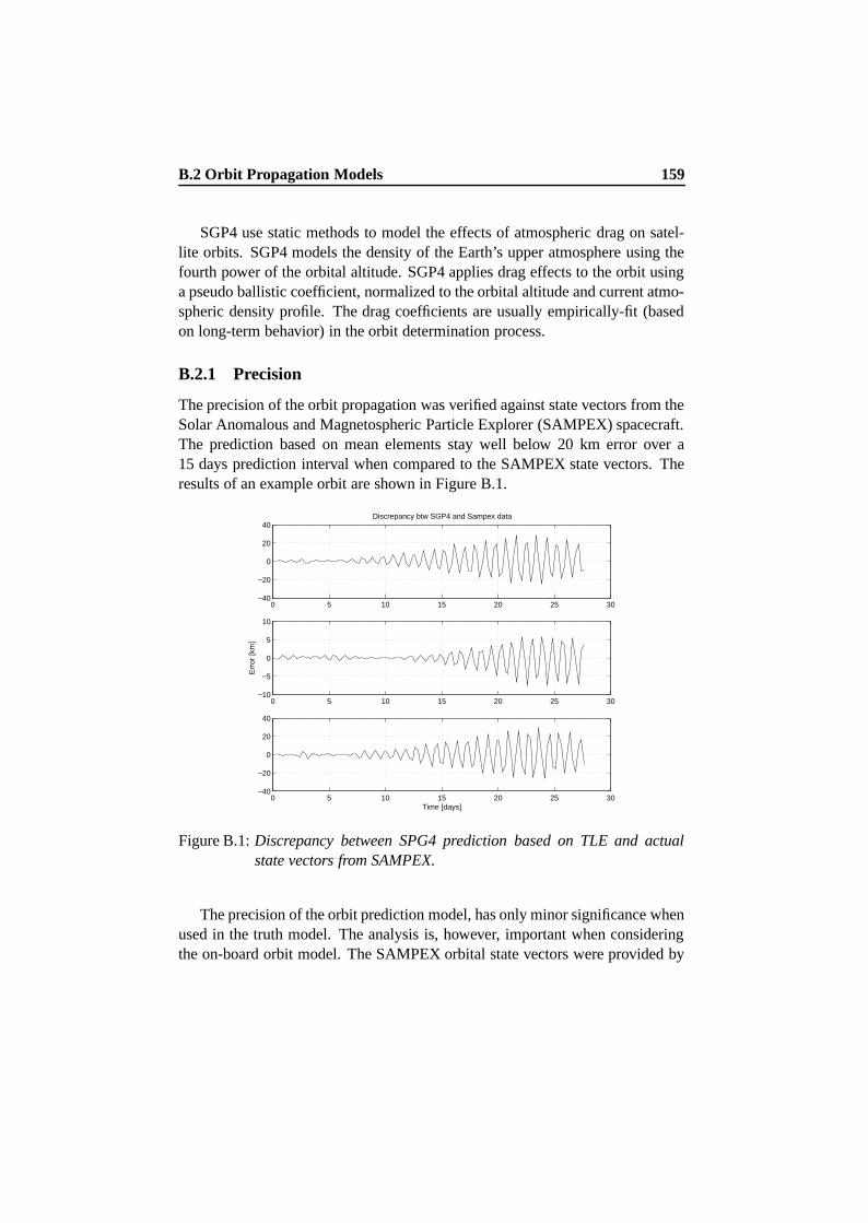
B.2 Orbit Propagation Models 159
SGP4 use static methods to model the effects of atmospheric drag on satel-lite orbits. SGP4 models the density of the Earth’s upper atmosphere using thefourth power of the orbital altitude. SGP4 applies drag effects to the orbit usinga pseudo ballistic coefficient, normalized to the orbital altitude and current atmo-spheric density profile. The drag coefficients are usually empirically-fit (basedon long-term behavior) in the orbit determination process.
B.2.1 Precision
The precision of the orbit propagation was verified against state vectors from theSolar Anomalous and Magnetospheric Particle Explorer (SAMPEX) spacecraft.The prediction based on mean elements stay well below 20 km error over a15 days prediction interval when compared to the SAMPEX state vectors. Theresults of an example orbit are shown in Figure B.1.
0 5 10 15 20 25 30−40
−20
0
20
40Discrepancy btw SGP4 and Sampex data
0 5 10 15 20 25 30−10
−5
0
5
10
Err
or [k
m]
0 5 10 15 20 25 30−40
−20
0
20
40
Time [days]
Figure B.1: Discrepancy between SPG4 prediction based on TLE and actualstate vectors from SAMPEX.
The precision of the orbit prediction model, has only minor significance whenused in the truth model. The analysis is, however, important when consideringthe on-board orbit model. The SAMPEX orbital state vectors were provided by
160 Satellite and Space Environmental Models
courtesy of H. Hoffmann, NASA Goddard Space Flight Center.
B.3 Geomagnetic Reference Field Model
As shown by Gauss in 1839, the main geomagnetic field (i.e., magnetic potential)can be represented by a spherical harmonic series, the first term being the simpledipole term. A gradient of the potential determines the magnetic vector field. TheEarth’s real magnetic field is the sum of several contributions including the main(core) field, the crustal (anomaly) field, and the external source (magnetospheric)fields.
The principal data sources for the main geomagnetic field modeling are thefollowing:
– Permanent (standard) magnetic observatories worldwide
– Global satellite magnetic measurements
– Magnetic surveys from the aircraft and ships
Satellite data (MAGSAT and Dynamic Explorer 2) have also helped to evalu-ate the crustal (anomaly) fields at individual observatories and regions and havethus greatly enhanced the accuracy of observatory data for the main field mod-eling. Temporal variations of the internal field have been modeled by expandingthe coefficients in a Taylor series in time. Most models include only the constantand first time derivative (secular variation) terms.
The International Geomagnetic Reference Field (IGRF) model is the em-pirical representation of the Earth’s magnetic field recommended for scientificuse by the International Association of Geomagnetism and Aeronomy. TheIGRF model represents the main (core) field without external sources. Theyemploy the usual spherical harmonics expansion of the scalar potential in geo-centric coordinates. The IGRF model coefficients are based on all available datasources including geomagnetic measurements from observatories, ships, aircraftand satellites.
Bibliography
Andre, M., (Ed.) (1993). The FREJA Scientific Satellite. Vol. IRF Scientific Re-port 214. 3 ed.. Swedish Institute of Space Physics.
Bak, T. (1994). Attitude Determination Methods. Technical Report ØrstedProject TN-151. Aalborg University.
Bak, T. (1995). Onboard Models for Autonomous Attitude Determination. TNT03-06-021. Aalborg University.
Bak, T. (1996). Onboard Attitude Determination for a Small Satellite. In proc.:Proceedings Third International Conference on Spacecraft Guidance, Navi-gation and Control Systems. ESA.
Bak, T. (1997). The Autonomous Formation Flying (AFF) Sensor. Engineringmemorandum. JPL.
Bak, T. (1998a). Attitude Reconstruction for FREJA, a Magnetometer based Ap-proach. In proc.: IFAC World Congress ’99.
Bak, T. (1998b). FREJA Attitude Estimation. Technical note R4246. AalborgUniversity.
Bak, T. and D. Bayard (1997). JPL Multipath Estimation Technique with aGeneric GPS Receiver. Technical Report Enginering Memorandum, EM-3455-97-034. JPL.
Bak, T. and R. Wisniewski (1996). Passive Aerodynamic Stabilization of a lowEarth orbit Satellite. In proc.: Proceedings Third International Conference onSpacecraft Guidance, Navigation and Control Systems. ESA.
Bak, T., H. H. Pedersen and C. Brøndum (1995). The Ørsted satellite with flexi-ble boom. Master’s thesis. Aalborg University.
161
162 BIBLIOGRAPHY
Bak, T., R. Wisniewski and M. Blanke (1996a). Autonomous Attitude Determi-nation and Control System for the Ørsted Satellite. In proc.: IEEE AerospaceApplication Conference.
Bak, T., R. Wisniewski and M. Blanke (1996b). Gso-l: Assessment of attitudedynamics. In: In ESA study on Geomagnetic Space Observatories (TorstenNeubert, Ed.). DMI/GSO/RPT/005.
Ballard, B. and J. Hayes (1992). FREJA F2 Magnetic Field Experiment SoftwareRequirements. Technical report. JHU/APL.
Bar-Itzhack, I. Y. (1996). REQUEST: A Recursive QUEST Algorithm for Se-quential Attitude Determination. Journal of Guidance, Control, and Dynamics19(5), 1034–1038.
Bar-Itzhack, I. Y. and R. R. Harman (1997). Optimized TRIAD Algorithmfor Attitude Determination. Journal of Guidance, Control, and Dynamics20(1), 208–211.
Bar-Itzhack, I. Y., L. Markley and J. Deutchmann (1991). Quaternion Narmaliza-tion in Additive EKF for Spacecraft Attitude Determination. In proc.: FlightMechanics/Estimation Symposium.
Bar-Itzhack, I.Y. and Y. Oshman (1985). Attitude Determination from VectorObservations: Quaternion Estimation. IEEE Transaction on Aerospace andElectronic Systems 21(1), 128–135.
Bar-Shalom, Y. and T.E. Fortmann (1988). Tracking and Data Association. TheAcademic Press.
Basseville, M. and I.V. Nikiforov (1993). Detection of Abrupt Changes: Theoryand Application. Prentice Hall. New Jersey.
Bauer, Peter (1999). Analysis of thermal effects on the Ørsted science data. Pre-liminary Report.
Bøgh, S. A. (1996). ACS Benchmarking. Ørsted/TN 331. AAU. Aalborg Uni-versity.
Bøgh, S. A. (1997). Fault Tolerant Control Systems - a Development Methodand Real-life Case Study. PhD thesis. Aalborg University.
BIBLIOGRAPHY 163
Bøgh, S. A., R. Wisniewski and T. Bak (1997). Autonomous Attitude ControlSystem for the Ørsted Satellite. In proc.: Proceedings of the IFAC Workshopon Control of Small Spacecraft, Breckenbridge, USA, Feb. ’97.
Bierman, G. J. (1977). Factorization Methods for Discrete Sequential Estima-tion. Vol. 128 of Mathematics in Science and Engineering. Academic Press.
Blanke, M. (1995). Aims and Tools in the Evolution of Fault-tolerant Control. Inproc.: ESF COSY Workshop, Rome.
Bøgh, S. A., R. Izadi-Zamanabadi and M. Blanke (1995). Onboard Supervisorfor the Ørsted Satellite Attitude Control System. In proc.: 5th ESA workshopon Artificial Inteligence and Knowledge Based Systems for Space.
Bryson, A. E. (1994). Control of spacecraft and aircraft. Princeton universitypress.
Bucy, R.S. and P.D. Joseph (1968). Filtering for Stochastic Processes, with Ap-plications to Guidance. Wiley. New York.
Challa, M. S. (1993). Solar, Anomalous and Magnetospheric Particle Explorer(SAMPEX) REal-Time Sequential Filter (RTSF). Evaluation report. NASAGoddard Space Flight Center.
Challa, M., S. Kotaru and G. Natanson (1997). Magnetometer-only Attitudeand Rate Estimates During the Earth Radiation Budget Satellite 1987 Con-trol Anomaly.
Chevalley, C. (1946). Theory of Lie Groups. Princeton University Press.
Clarke, D. S., M. T. Hicks, A. M. Fitzgerald, J. J. Suchman, R. J. Twiggs, J. Ran-dolf and T. W. Kenny (1996). Picosat Free Flying Magnetometer Experiments.In proc.: 10th Anual AIAA Small Satellite Conference.
Cohen, C. E. (1992). Attitude Determination Using GPS. PhD thesis. StanfordUniversity, Department of Aeronautics and Astronautics.
Crassidis, J. L. and F. L. Markley (1997a). Minimum Model Error Ap-proach for Attitude Estimation. Journal of Guidance, Control, and Dynamics20(6), 1241–1247.
164 BIBLIOGRAPHY
Crassidis, J. L. and F. L. Markley (1997b). Predictive Filtering for Attitude Es-timation Without Rate Sensors. Journal of Guidance, Control, and Dynamics20(3), 522–527.
Deutchmann, J., R. Harman and I. Bar-Itzhack (1998). A Low Cost Approach toSimultaneous Orbit, Attitude, and Rate Estimation Using an Extended KalmanFilter. In proc.: AAS/GSFC 13th International Symposium on Space FlightDynamics (Tom Stengle, Ed.). Vol. 2. pp. 667–676.
Eisenman, A., C. C. Liebe and J. Jørgensen (1996). Astronomical Performanceof the Engineering Model of Ørsted Advanced Stellar Compass. In proc.:Space Sciencecraft Control and Tracking in the New Millennium (E. KaneCasani and Mark A. Vander Does, Eds.). pp. 252–264.
Fisher, H. L., M. D. Shuster and T. E. Strikwerda (1989). Attitude Determinationfor the Star Tracker Mission. In proc.: AAS/AIAA Astrodynamics Conference.Orlando, Florida. pp. 139–150.
Flatley, T. W., J. K. Forden, D. A. Henretty, E. G. Lightsey and F. L. Markley(1990). On-board Attitude Determination and Control Algorithms for SAM-PEX. In proc.: Flight Mechanics/Estimation Theory Symposium.
Gai, E., K. Daly, J. Harrison and L. Lemos (1985). Star-Sensor-Based SatelliteAttitude/Attitude Rate Estimator. Journal of Guidance, Control, and Dynam-ics 8(5), 560–565.
Goldstein, H. (1950). Classical Mechanics. Addison-Wesley. Reading, Mas-sachusetts.
Grewal, M. S. and A. P. Andrews (1993). Kalman Filtering, Theory and Practice.Information and System Science Series. Prentice Hall.
Hamilton, W. R. (1866). Elements of Quaternions. Longmans, Green. London.
Handschin, J. E. (1970). Monte Carlo Techniques for Prediction and Filtering ofNon-linear Stochastic Processes. Automatica 6(4), 555–563.
Hedin, A. E. (1987). MSIS-86 Thermospheric Model. J. Geophys. Res. 92.
Hoots, F. R. and R. L. Roehrich (1980). Models for Propagation of NORADElement Sets. Technical report. Spacetrack report no.3.
BIBLIOGRAPHY 165
Hughes, P. C. (1986). Spacecraft Attitude Dynamics. Wiley and Sons, Inc.
ISSD (1999). Internet supported space database, http://issd.zarm.uni-bremen.de/. University Of Bremen, Germany.
Jakubczyk, B. and W. Respondek (1999). Geometric Nonlinear Control. Lec-ture notes, Aalborg University, Department of Control Engineering. Aalborg,Denmark.
Jazwinski, A. H. (1970). Stochastic Processes and Filtering Theory. Vol. 64 ofMathematics in science and engineering. Academic Press, Inc.. London.
Jørgensen, J.L. (1995). Development of the Ørsted Precision Attitude Instrumentthe Star Imager. In proc.: The Chapman Conf. on Measurement Techniques forSpace Plasmas.
Kalman, R. E. (1960). A new approach to linear filtering and prediction prob-lems. Transaction of ASME, Series D, Journal of Basic Engineering 82, 35–45.
Kane, T. R., P. W. Likins and D. A. Levinson (1983). Spacecraft Dynamics.McGraw-Hill.
Langel, R. A. (1987). The main geomagnetic field. In: Geomagnetism (J. A.Jacobs, Ed.). Chap. 4, pp. 249–512. Academic Press.
Larson, W. J. and Wertz, J. R., Eds.) (1992). Space Mission Analysis and Design.Luwer Academic Publishers.
Lefferts, E. J., F. L. Markley and M. D. Shuster (1982). Kalman Filteringfor Spacecraft Attitude Determination. Journal of Guidance and Control5(5), 417–429.
Lerner, G.M. (1978). Spacecraft Attitude Determination and Control. Chap.Three-Axis Attitude Determination, pp. 420–428. Reidel, Dordrecht, TheNetherlands.
Liebe, C. C. (1995). Star Trackers for Attitude Determination. IEEE Aerospaceand Electronic Systems Magazine 10(6), 10–16.
Lightsey, E. G., E. E. Cohen, W .A. Feess and B. W. Parkinson (94). Analy-sis os spacecraft attitude Measurements using onboard GPS. Advances in theAstronautical Sciences 86, 521–532.
166 BIBLIOGRAPHY
Ljung, L. (1979). Asymptotic Behavior of the Extended Kalman Filter as a Pa-rameter Estimator for Linear Systems. 24(1), 36–50.
Ljung, L. (1987). System Identification, Theory for the User. Prentice-Hall in-formation and system sciences series. Prentice-Hall.
Luehr, H. (1997). Magnetfeldmessungen auf dem schwedish-deutchen SatellitenFREJA. Technical report. Technischen Universitaet Braunschweig.
Markley, F. L. (1988). Attitude Determination Using Vector Observations andthe Singular Value Decomposition. Journal of the Astronautical Sciences36(3), 245–258.
Markley, F. L. (1993). Attitude Determination Using Vector Observations:A Fast Optimal Matrix Algorithm. Journal of the Astronautical Sciences41(2), 261–280.
Maybeck, P. S. (1979a). Stochastic Models, Estimation, and Control. Vol. 1.Academic Press.
Maybeck, P. S. (1979b). Stochastic Models, Estimation, and Control. Vol. 2.Academic Press.
Melvin, P.J. and A. S. Hope (1993). Satellite attitude determination with GPS.Advances in the Astronautical Sciences 85, 59–78.
Natanson, G. (1993). A Deterministic Method for Estimating Attitude FromMagnetometer Data. In proc.: 43rd Congress of the International Astronauti-cal Federation.
Nielsen, O. V., B. Hernando, J.R. Petersen and F. Primdahl (1990). Miniaturisa-tion of Low-Cost Metalic Glass Flux-Gate Sensors. Magnetism and MagneticMaterials 83, 404–406.
Nijmeijer, H. and T. I. Fossen (1999). New Directions in Nonlinear Observer De-sign. Vol. 244 of Lecture Notes in Control and Information Sciences. Springer-Verlag.
Oshman, Y. (1999). Private Communication.
Oshman, Y. and F. L. Markley (1999). Sequential Attitude and Attitude-Rate Es-timation Using Integrated-Rate Parameters. Journal of the Astronautical Sci-ences 22(3), 385–394.
BIBLIOGRAPHY 167
Overschee, P. Van and B. De Moor (1996). Subspace Identification for LinearSystems: Theory-Implementation-Applications. Kluwer Academic Publishers.
Padgett, C., K. Kreutz-Delgado and S. Udomkesmalee (1997). Evaluation ofStar Identification Techniques. Journal of Guidance, control, and Dynamics20(2), 259–267.
Primdahl, F. and P. A. Jensen (1984). Dansk Rumforskningsinstitut’s raket mag-netometer eksperiment (in danish). Gamma, Tidskrift for fysik.
Psiaki, M. L., F. Martel and P. K. Pal (1990). Three-Axis Attitude Determinationvia Kalman Filtering of Magnetometer Data. Journal of Guidance, Controland Dynamics 13(3), 506–514.
Rauch, H. E., F. Tung and C.T. Striebel (1965). Maximum likelihood estimatesof linear dynamic systems. AIAA Journal 3(8), 1445–1450.
Reigber, C., (Ed.) (1996). Champ, Phase B. Scientific technical reportSTR96/13. champ project office.
Schei, T. S. (1997). A Finite-Difference Method for Linearization in NonlinearEstimation Algorithms. Automatica.
Shuster, M. D. (1989). A Simple Kalman Filter and Smoother for SpacecraftAttitude. Journal of the Astronautical Sciences 37(1), 89–106.
Shuster, M. D. (1993). A Survey of Atttitude Representations. Journal of theAstronautical Sciences.
Shuster, M. D. and S.D Oh (1981). Attitude Determination from Vector Obser-vations. Journal of Guidance and Control 4(1), 70–77.
Stuelpnagel, J. D. (1964). On the Parametrization of the three-dimensional rota-tion group. SIAM review 6, 422–430.
Thornton, C.L. (1976). Triangular Covariance Factorization for Kalman Filter-ing. Ph.d. thesis. University of California at Los Angeles.
Wahba, G. (1965). A Least Squares Estimate of Satellite Attitude. SIAM Review7(3), 409.
Wertz, J. R., (Ed.) (1978). Spacecraft Attitude Determination and Control.Kluwer Academic Publishers.

168 BIBLIOGRAPHY
Wisniewski, R. (1997). Satellite Attitude Control Using Only Magnetic Actua-tion. PhD thesis. Aalborg University.
Zhou, W.-W. and M. Blanke (1989). Idenfitication of a Class of Nonlinear State-Space Models Using RPE Techniques. IEEE Transaction on Automatic Con-trol 34(3), 312–316.