Decentralized Coordinated Attitude Control of aFormation of Spacecraft

by

Matthew C. VanDyke

Thesis submitted to the Faculty of the

Virginia Polytechnic Institute and State University

in partial fulfillment of the requirements for the degree of

Master of Science

in

Aerospace Engineering

Dr. Christopher D. Hall, Committee Chair

Dr. Hanspeter Schaub, Committee Member

Dr. Naira Hovakimyan, Committee Member

May 21, 2004

Blacksburg, Virginia

Keywords: spacecraft, dynamics, control, decentralized, coordinated, Liaponuv, nonlinear,

formation, attitude, behavior-based

Copyright 2004, Matthew C. VanDyke

Abstract

Decentralized Coordinated Attitude Control of a Formation of

Spacecraft

Matthew Clark VanDyke

Spacecraft formations offer more powerful and robust space system architectures than single

spacecraft systems. Investigations into the dynamics and control of spacecraft formations

are vital for the development and design of future successful space missions. The problem of

controlling the attitude of a formation of spacecraft is investigated. The spacecraft formation

is modelled as a distributed system, where the individual spacecraft’s attitude control systems

are the local control agents. A decentralized attitude controller utilizing behavior-based

control is developed. The global stability of the controller is proven using Lyaponuv stability

theory. Convergence of the attitude controller is proven through the use of an invariance

argument. The attitude controller’s stability and convergence characteristics are investigated

further through numeric simulation of the attitude dynamics of the spacecraft formation.

Dedication & Acknowledgements

I dedicate this work to my beautiful fiancee Melissa, who had to withstand two years of

separation from me because of it. How she was ever able to summon the courage and fortitude

necessary to withstand such a tremendous sacrifice, I may never know. I also dedicate some

small portion of this work (perhaps just the references) to the past and present inhabitants∗

of the Space Systems Simulation Laboratory, whose ability to divert my attention from my

work (with such wonderfully silly things as lunch and demerits) was invaluable in the delay

to get it done. I would like to thank my advisor, Dr. Hall, for his guidance in this research

and without whom this manuscript would not be the sparkling example of perfection that

you see before you. And finally, I would like to thank the Virginia Space Grant Consortium

who generously partially funded this research.

∗In loose chronological order: Jana Schwartz, Matt Berry, Scott Lennox, Marcus Pressl, Andrew Turner,Eugene Skelton, Mike Shoemaker, Brett Streetman, Sam Wright, Justin McFarland

iii

Contents

1 Introduction 1

1.1 Spacecraft Formation Flying . . . . . . . . . . . . . . . . . . . . . . . . . . . 2

1.2 Coordinated Control . . . . . . . . . . . . . . . . . . . . . . . . . . . . . . . 2

1.3 Behavior-Based Control . . . . . . . . . . . . . . . . . . . . . . . . . . . . . 4

1.4 Applications . . . . . . . . . . . . . . . . . . . . . . . . . . . . . . . . . . . . 5

1.4.1 Interferometry . . . . . . . . . . . . . . . . . . . . . . . . . . . . . . . 5

1.4.2 Spacecraft Orbital Formation-Keeping . . . . . . . . . . . . . . . . . 5

1.5 Outline of Thesis . . . . . . . . . . . . . . . . . . . . . . . . . . . . . . . . . 6

2 Literature Review 7

2.1 Wang, Hadaegh, Yee, and Lau - The First School . . . . . . . . . . . . . . . 7

2.2 Lawton, Beard, Hadaegh, and Ren - The Second School . . . . . . . . . . . . 8

2.3 Kang, Yeh, and Sparks - The Third School . . . . . . . . . . . . . . . . . . . 10

2.4 Deficiencies in the Literature . . . . . . . . . . . . . . . . . . . . . . . . . . . 11

2.5 Summary and Conclusions . . . . . . . . . . . . . . . . . . . . . . . . . . . . 11

3 Spacecraft Attitude Dynamics 12

iii

3.1 Vectors and Reference Frames . . . . . . . . . . . . . . . . . . . . . . . . . . 12

3.2 Attitude Representations . . . . . . . . . . . . . . . . . . . . . . . . . . . . . 14

3.2.1 Rotation Matrices . . . . . . . . . . . . . . . . . . . . . . . . . . . . . 14

3.2.2 Quaternions . . . . . . . . . . . . . . . . . . . . . . . . . . . . . . . . 17

3.3 Equations of Motion . . . . . . . . . . . . . . . . . . . . . . . . . . . . . . . 18

3.4 Attitude Error Dynamics . . . . . . . . . . . . . . . . . . . . . . . . . . . . . 19

3.4.1 Station-Keeping Error . . . . . . . . . . . . . . . . . . . . . . . . . . 19

3.4.2 Formation-Keeping Error . . . . . . . . . . . . . . . . . . . . . . . . . 20

3.5 Summary . . . . . . . . . . . . . . . . . . . . . . . . . . . . . . . . . . . . . 21

4 Spacecraft Attitude Control 22

4.1 Lyapunov Stability Theory . . . . . . . . . . . . . . . . . . . . . . . . . . . . 22

4.2 Quaternion-Based Attitude Controller . . . . . . . . . . . . . . . . . . . . . . 25

4.2.1 Simulation Results . . . . . . . . . . . . . . . . . . . . . . . . . . . . 26

4.3 Quaternion-Based Attitude Tracking Controller . . . . . . . . . . . . . . . . 28

4.3.1 Simulation Results . . . . . . . . . . . . . . . . . . . . . . . . . . . . 30

4.4 Summary . . . . . . . . . . . . . . . . . . . . . . . . . . . . . . . . . . . . . 31

5 Spacecraft Formation Attitude Control 34

5.1 Problem Statement . . . . . . . . . . . . . . . . . . . . . . . . . . . . . . . . 34

5.1.1 Approach . . . . . . . . . . . . . . . . . . . . . . . . . . . . . . . . . 35

5.1.2 Assumptions . . . . . . . . . . . . . . . . . . . . . . . . . . . . . . . . 36

5.1.3 Scope of Research . . . . . . . . . . . . . . . . . . . . . . . . . . . . . 37

iv

5.2 The Decentralized Coordinated Attitude Controller . . . . . . . . . . . . . . 37

5.2.1 Desired Behavior Control Actions . . . . . . . . . . . . . . . . . . . . 37

5.2.2 The Control Law . . . . . . . . . . . . . . . . . . . . . . . . . . . . . 38

5.3 Coordination Architectures . . . . . . . . . . . . . . . . . . . . . . . . . . . . 39

5.4 Global Stability and Convergence Proofs . . . . . . . . . . . . . . . . . . . . 42

5.5 Summary . . . . . . . . . . . . . . . . . . . . . . . . . . . . . . . . . . . . . 47

6 Simulation Results 48

6.1 Common Simulation Parameters . . . . . . . . . . . . . . . . . . . . . . . . . 48

6.2 Nominal Case . . . . . . . . . . . . . . . . . . . . . . . . . . . . . . . . . . . 52

6.3 Differing Coordination Architectures . . . . . . . . . . . . . . . . . . . . . . 53

6.3.1 Behavior Weighting Variation . . . . . . . . . . . . . . . . . . . . . . 53

6.3.2 Spacecraft Connection Variations . . . . . . . . . . . . . . . . . . . . 56

6.3.3 Cluster Coordination Architectures . . . . . . . . . . . . . . . . . . . 59

6.4 Gravity-Gradient Torque . . . . . . . . . . . . . . . . . . . . . . . . . . . . . 62

6.5 Summary . . . . . . . . . . . . . . . . . . . . . . . . . . . . . . . . . . . . . 65

7 Summary & Conclusions 69

v

List of Figures

1.1 A general depiction of the (A) centralized and (B) decentralized coordinated

control types. . . . . . . . . . . . . . . . . . . . . . . . . . . . . . . . . . . . 3

1.2 An example where a goal attainment behavior and an obstacle avoidance

behavior conflict. . . . . . . . . . . . . . . . . . . . . . . . . . . . . . . . . . 4

3.1 The kth reference frame, Fk, consisting of the triad of ~k1, ~k2, and ~k3 . . . . 13

3.2 The vector ~v shown in the kth reference frame, Fk . . . . . . . . . . . . . . . 14

3.3 The unit reference vectors of Fj and Fk . . . . . . . . . . . . . . . . . . . . . 15

4.1 Angular error of the spacecraft during the simulation . . . . . . . . . . . . . 27

4.2 Angular rate error of the spacecraft during the simulation . . . . . . . . . . . 28

4.3 Magnitude of the control torque applied during the simulation . . . . . . . . 28

4.4 Angular error of the spacecraft tracking an attitude trajectory during the

simulation . . . . . . . . . . . . . . . . . . . . . . . . . . . . . . . . . . . . . 31

4.5 Angular rate error of the spacecraft tracking an attitude trajectory during the

simulation . . . . . . . . . . . . . . . . . . . . . . . . . . . . . . . . . . . . . 32

4.6 Magnitude of the control torque applied during the simulation of the space-

craft tracking an attitude trajectory . . . . . . . . . . . . . . . . . . . . . . . 32

vi

5.1 Four decentralized coordination architectures using a different number of con-

nections between spacecraft in the formation . . . . . . . . . . . . . . . . . . 40

5.2 A coordination architecture where the individual spacecraft do not all have

the same number of connections . . . . . . . . . . . . . . . . . . . . . . . . . 41

5.3 A spacecraft that is connected to four other spacecraft in the formation using

different weights . . . . . . . . . . . . . . . . . . . . . . . . . . . . . . . . . . 41

5.4 A decentralized coordination architecture that groups spacecraft into clusters 42

6.1 Attitude trajectory of the reference spacecraft . . . . . . . . . . . . . . . . . 49

6.2 The simulation results of a spacecraft formation using the quaternion-based

decentralized controller . . . . . . . . . . . . . . . . . . . . . . . . . . . . . . 52

6.3 Relative angular error performance of the spacecraft formation using different

values of the formation-keeping behavior weighting . . . . . . . . . . . . . . 54

6.4 Absolute angular error performance of the spacecraft formation using different

values of the formation-keeping behavior weighting . . . . . . . . . . . . . . 55

6.5 Average control torque magnitude applied by the spacecraft in the formation

using different values of the formation-keeping behavior weighting . . . . . . 56

6.6 Relative angular error performance of the spacecraft formation using different

numbers of connections between spacecraft . . . . . . . . . . . . . . . . . . . 57

6.7 Absolute angular error performance of the spacecraft formation using different

numbers of connections between spacecraft . . . . . . . . . . . . . . . . . . . 58

6.8 Average control torque magnitude applied by the spacecraft in the formation

using different numbers of connections between spacecraft . . . . . . . . . . . 59

6.9 Simulation results of a spacecraft formation using a cluster-type coordination

architecture . . . . . . . . . . . . . . . . . . . . . . . . . . . . . . . . . . . . 61

6.10 Relative angular error results of a spacecraft formation using a cluster-type

coordination architecture . . . . . . . . . . . . . . . . . . . . . . . . . . . . . 62

vii

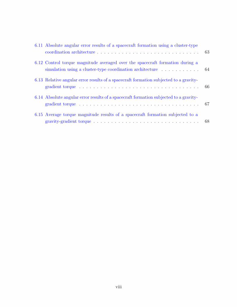
6.11 Absolute angular error results of a spacecraft formation using a cluster-type

coordination architecture . . . . . . . . . . . . . . . . . . . . . . . . . . . . . 63

6.12 Control torque magnitude averaged over the spacecraft formation during a

simulation using a cluster-type coordination architecture . . . . . . . . . . . 64

6.13 Relative angular error results of a spacecraft formation subjected to a gravity-

gradient torque . . . . . . . . . . . . . . . . . . . . . . . . . . . . . . . . . . 66

6.14 Absolute angular error results of a spacecraft formation subjected to a gravity-

gradient torque . . . . . . . . . . . . . . . . . . . . . . . . . . . . . . . . . . 67

6.15 Average torque magnitude results of a spacecraft formation subjected to a

gravity-gradient torque . . . . . . . . . . . . . . . . . . . . . . . . . . . . . . 68

viii

List of Tables

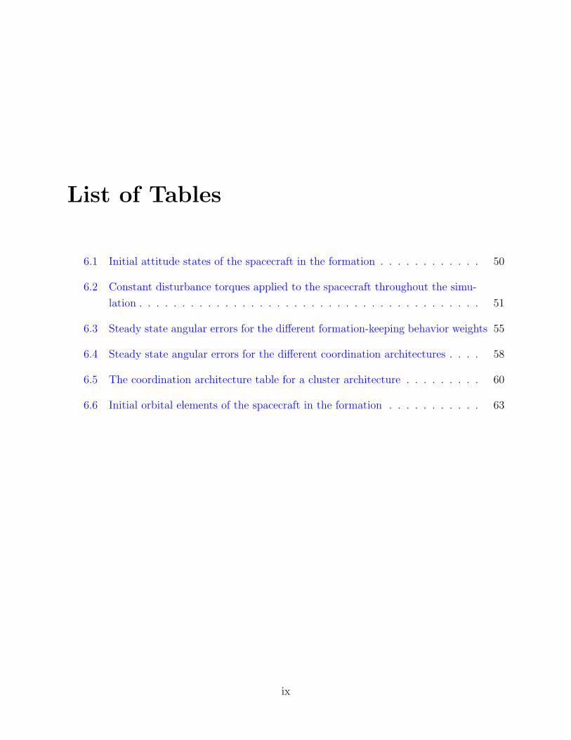
6.1 Initial attitude states of the spacecraft in the formation . . . . . . . . . . . . 50

6.2 Constant disturbance torques applied to the spacecraft throughout the simu-

lation . . . . . . . . . . . . . . . . . . . . . . . . . . . . . . . . . . . . . . . . 51

6.3 Steady state angular errors for the different formation-keeping behavior weights 55

6.4 Steady state angular errors for the different coordination architectures . . . . 58

6.5 The coordination architecture table for a cluster architecture . . . . . . . . . 60

6.6 Initial orbital elements of the spacecraft in the formation . . . . . . . . . . . 63

ix

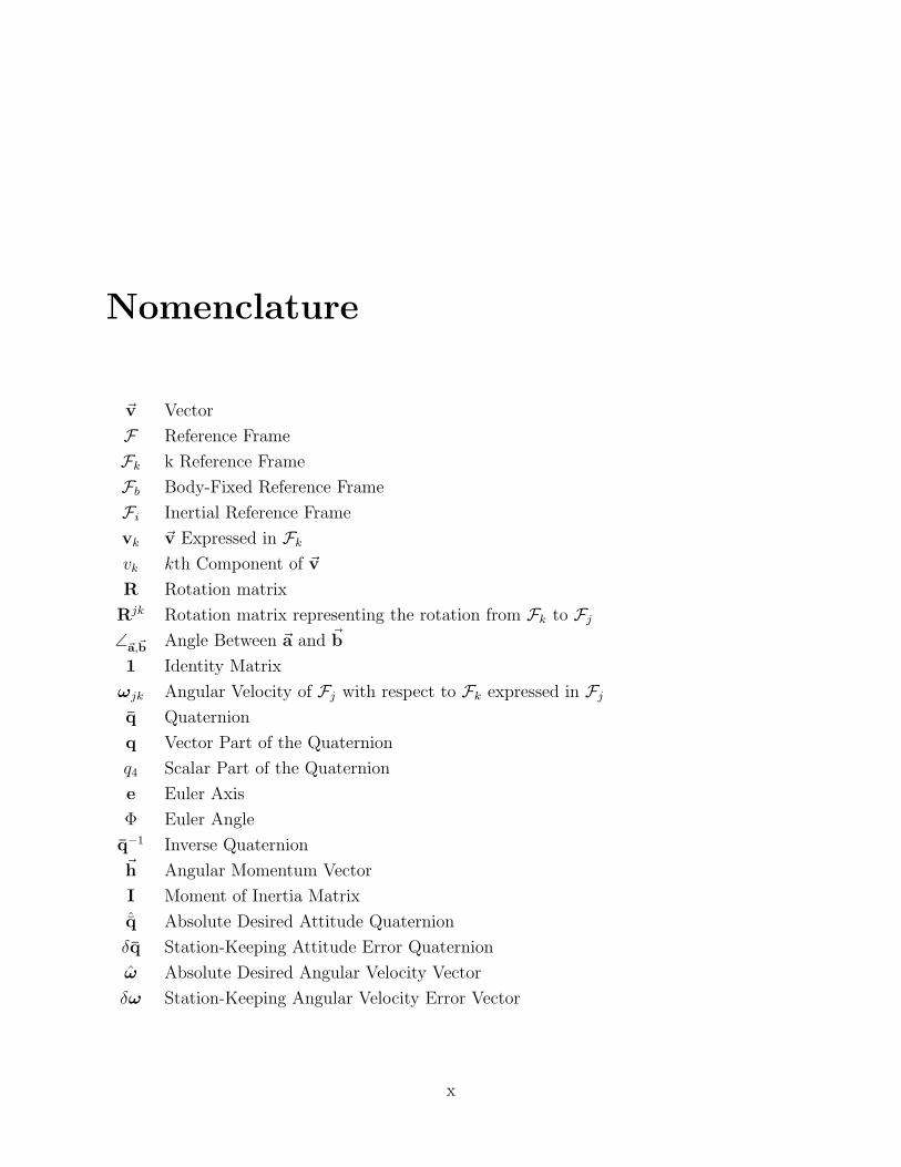
Nomenclature

~v Vector

F Reference Frame

Fk k Reference Frame

Fb Body-Fixed Reference Frame

Fi Inertial Reference Frame

vk ~v Expressed in Fk

vk kth Component of ~v

R Rotation matrix

Rjk Rotation matrix representing the rotation from Fk to Fj

∠~a,~b Angle Between ~a and ~b

1 Identity Matrix

ωjk Angular Velocity of Fj with respect to Fk expressed in Fj

q Quaternion

q Vector Part of the Quaternion

q4 Scalar Part of the Quaternion

e Euler Axis

Φ Euler Angle

q−1 Inverse Quaternion~h Angular Momentum Vector

I Moment of Inertia Matrix

ˆq Absolute Desired Attitude Quaternion

δq Station-Keeping Attitude Error Quaternion

ω Absolute Desired Angular Velocity Vector

δω Station-Keeping Angular Velocity Error Vector

x

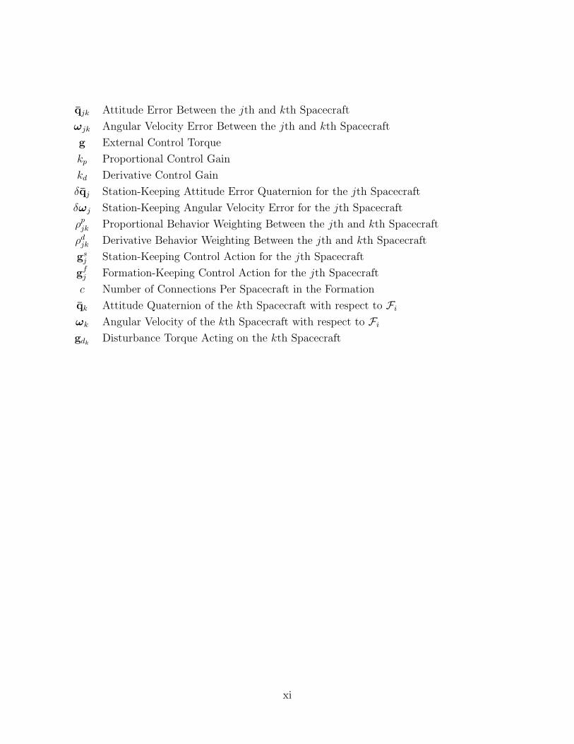
qjk Attitude Error Between the jth and kth Spacecraft

ωjk Angular Velocity Error Between the jth and kth Spacecraft

g External Control Torque

kp Proportional Control Gain

kd Derivative Control Gain

δqj Station-Keeping Attitude Error Quaternion for the jth Spacecraft

δωj Station-Keeping Angular Velocity Error for the jth Spacecraft

ρpjk Proportional Behavior Weighting Between the jth and kth Spacecraft

ρdjk Derivative Behavior Weighting Between the jth and kth Spacecraft

gsj Station-Keeping Control Action for the jth Spacecraft

gfj Formation-Keeping Control Action for the jth Spacecraft

c Number of Connections Per Spacecraft in the Formation

qk Attitude Quaternion of the kth Spacecraft with respect to Fi

ωk Angular Velocity of the kth Spacecraft with respect to Fi

gdkDisturbance Torque Acting on the kth Spacecraft

xi

1

Chapter 1

Introduction

The topic of spacecraft formation flying has pervaded much of the recent work in the space-

craft dynamics and control field. The reason for the recent focus is the power and flexibility

available to space system architectures that use spacecraft formations. Much of the work

has concentrated on translational control of the spacecraft in the formation. However, some

work has explored the problem of controlling the attitude of a spacecraft formation. Both

centralized and decentralized coordination approaches to the problem have been analyzed.

The centralized coordination approaches have been examined in detail;1–9 however there are

still gaps in the decentralized coordination approach literature.10–14 The most notable gap

is the lack of a decentralized coordinated attitude controller that guarantees global conver-

gence of the spacecraft formation. The research presented here extends the previous work

in decentralized coordinated attitude control. A class of decentralized coordinated attitude

control laws that guarantees global converge of the spacecraft formation is developed and

analyzed.

Three basic concepts important in the study of spacecraft formation attitude control are

spacecraft formation flying, coordinated control, and behavior-based control. These concepts

are briefly introduced and their relevance discussed.

1.1. SPACECRAFT FORMATION FLYING 2

1.1 Spacecraft Formation Flying

A spacecraft formation consists of two or more spacecraft in specific relative positions and

orientations. Dispersing the functions of a single spacecraft over a formation of spacecraft

produces a robust, fault-tolerant system architecture. The failure of a single spacecraft

in a formation does not necessarily lead to system failures as it would in a single, larger

spacecraft. Upgrades or repairs could be performed by simply replacing any obsolete or

disabled spacecraft.15 The cost of repair and upgrades of the system is reduced because of

the natural modularity of a spacecraft formation.

Spacecraft formations allow for higher performing and more efficient system architectures. A

formation facilitates greater resolution through the use of spatially distributed simultaneous

measurements.16 Long-baseline optical interferometry is an example of a high performance

system that requires distributed measurements.17 Another benefit of spacecraft formations

is their ability to change the relative spacecraft positions and attitudes to achieve optimal

configurations for different missions throughout the lifetime of the system. The result is a

system with greater functionality than a system consisting of a single spacecraft.15

1.2 Coordinated Control

A spacecraft formation is a distributed system. A distributed system is a large system

consisting of multiple smaller subsystems. The attitude control systems of the individual

spacecraft act as the local control agents. The control decisions of the local control agents

must be coordinated to ensure the stability and convergence of the global system.

Coordinated controllers are generally categorized into centralized and decentralized types.

The distinction is based on where the control decisions are made. Centralized control is

a type of coordinated control where a single control agent, called the global control agent,

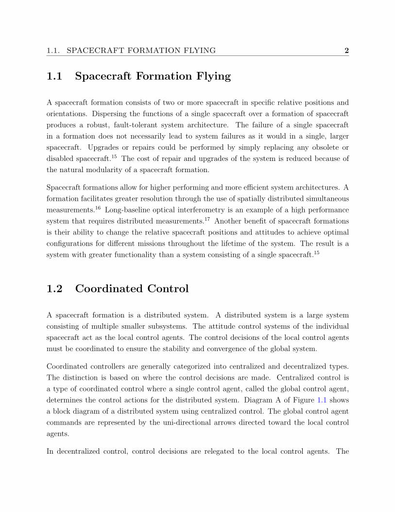
determines the control actions for the distributed system. Diagram A of Figure 1.1 shows

a block diagram of a distributed system using centralized control. The global control agent

commands are represented by the uni-directional arrows directed toward the local control

agents.

In decentralized control, control decisions are relegated to the local control agents. The

1.2. COORDINATED CONTROL 3

Figure 1.1: A general depiction of the (A) centralized and (B) decentralized coordinated control

types.

local control agents use local observations and any information communicated by the other

control agents to determine control actions. A block diagram of a distributed system using

decentralized control is presented in Part B of Figure 1.1. The bi-directional arrows represent

the two-way communication of information between the local control agents.

The two primary benefits of decentralized control over centralized control are fault-tolerance

and simpler control laws. Failure of a single local control agent in a decentralized controlled

system does not lead to the destabilization of the entire system.18 The failure is confined

to the region of the failed local control agent resulting in a graceful degradation of system

performance. Decentralized control results in relatively simple control laws, because the

design of the global controller can be decomposed into smaller control agents. The local

control agents are designed so that they perform their local control tasks, and coordinate

with one another to control the global system.18 The coordination is implemented by means

of communication between the local control agents. Centralized controllers require greater

information and information processing than what is required by the local control agents of

the equivalent decentralized controller.19 The primary drawback of decentralized controllers

is that they are difficult to analyze analytically.

1.3. BEHAVIOR-BASED CONTROL 4

1.3 Behavior-Based Control

A useful tool for the spacecraft formation attitude control problem is behavior-based con-

trol. Behavior-based control is implemented when a control system has multiple, and some-

times competing, objectives or behaviors. The behaviors could include goal-attainment,

collision-avoidance, obstacle-avoidance, and formation-keeping. The overall control action is

determined by a weighted sum of the control actions for each of the behaviors.20

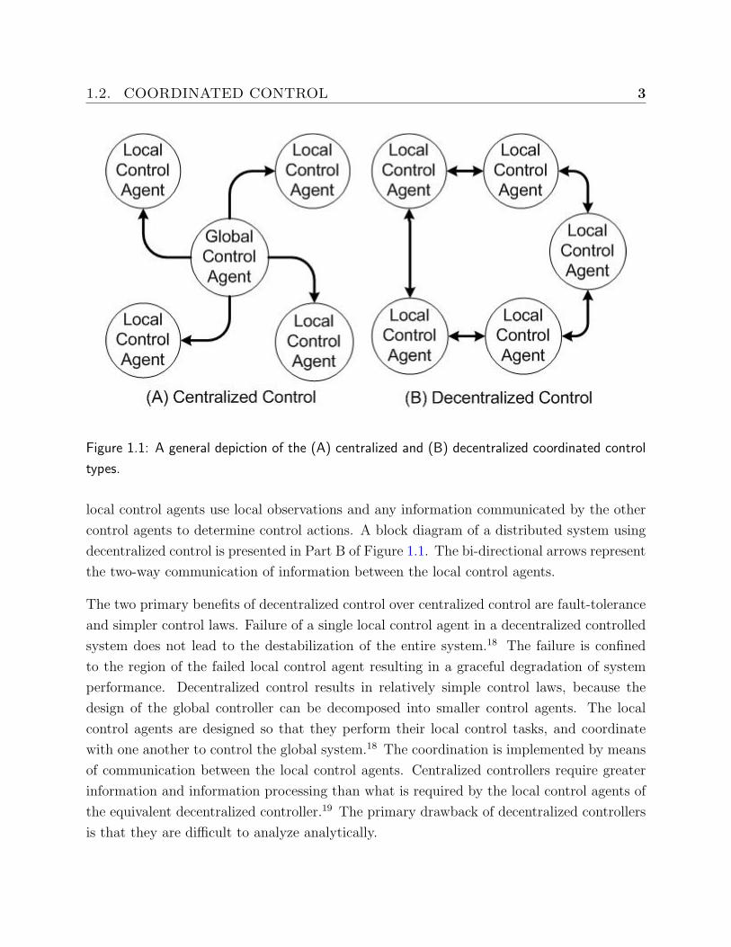
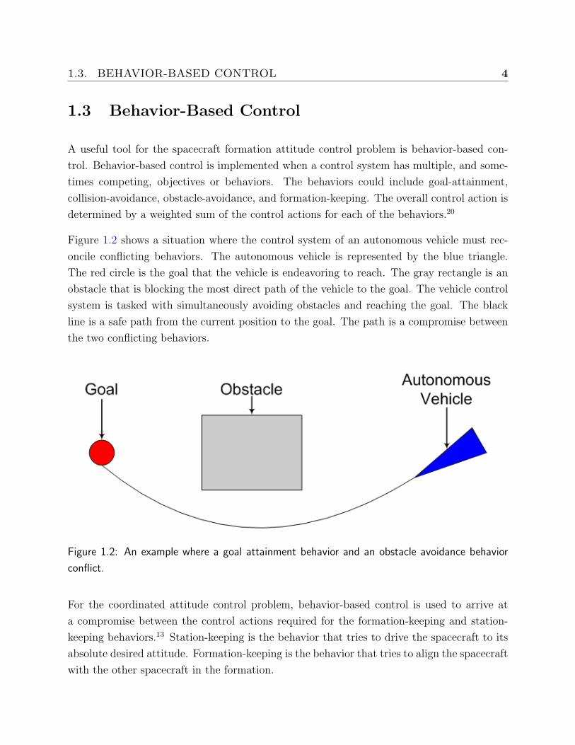
Figure 1.2 shows a situation where the control system of an autonomous vehicle must rec-

oncile conflicting behaviors. The autonomous vehicle is represented by the blue triangle.

The red circle is the goal that the vehicle is endeavoring to reach. The gray rectangle is an

obstacle that is blocking the most direct path of the vehicle to the goal. The vehicle control

system is tasked with simultaneously avoiding obstacles and reaching the goal. The black

line is a safe path from the current position to the goal. The path is a compromise between

the two conflicting behaviors.

Figure 1.2: An example where a goal attainment behavior and an obstacle avoidance behavior

conflict.

For the coordinated attitude control problem, behavior-based control is used to arrive at

a compromise between the control actions required for the formation-keeping and station-

keeping behaviors.13 Station-keeping is the behavior that tries to drive the spacecraft to its

absolute desired attitude. Formation-keeping is the behavior that tries to align the spacecraft

with the other spacecraft in the formation.

1.4. APPLICATIONS 5

1.4 Applications

Research into coordinated attitude control algorithms is applicable to any spacecraft forma-

tion flying mission. Improvements in attitude control generally lead to heightened overall

system performance. Two interesting applications of this research are long baseline interfer-

ometry and spacecraft positional formation-keeping.

1.4.1 Interferometry

Interferometry is being considered as a method to detect extra-solar planets for the Ter-

restrial Planet Finder (TPF). Interferometry would allow the cancellation of exo-zodiacal

light from the planet’s signal, thereby providing a better signal from which scientific data

can be extracted. One of the concepts being considered for the TPF uses a formation of

free-flying spacecraft, separated by hundreds of meters, equipped with optical sensors acting

as an interferometer.21

Interferometry using a spacecraft formation would require two or more spacecraft to move

within an observation plane to reflect light sampled from a celestial body to another space-

craft. Scientific data can then be extracted from the interference pattern of the sampled

light.10 A free-flying spacecraft interferometer provides better performance than a struc-

turally connected interferometer by allowing greater baselines, leading to greater resolutions,

and more complex nulling patterns to better cancel unwanted light.21

1.4.2 Spacecraft Orbital Formation-Keeping

Coordinated attitude control allows spacecraft in Low Earth Orbit (LEO) to maintain tighter

formations. Spacecraft formations in LEO are subject to an atmospheric drag force. The

drag force has a disturbing influence on spacecraft formations. Even if the spacecraft are

identical, the drag force experienced by each is slightly different. The difference is caused

by the relative attitude tracking errors of the spacecraft. The relative attitude error causes

the spacecraft to have different attitudes with respect to their velocity vectors, and therefore

with respect to the free-stream. The differences in the attitudes of the spacecraft with

respect to the free-stream results in differing drag forces. Therefore, a spacecraft formation

1.5. OUTLINE OF THESIS 6

with smaller relative attitude error is less affected by the drag force disturbance, thereby

lessening the propulsive force required to maintain the formation.22

1.5 Outline of Thesis

A review of the literature specifically related to the topic of coordinated attitude control is

presented in Chapter 2. The literature is grouped into three categories based on the approach

used by the authors. Deficiencies in the literature are noted for later resolution.

A review of spacecraft dynamics is given in Chapter 3. Absolute and relative attitude

kinematic error variables for the spacecraft are formulated. Chapter 4 discusses nonlinear

attitude control of a spacecraft modelled as a rigid body. Stability definitions and theorems

are introduced and used to develop two quaternion-based attitude controllers. The primary

contribution of this work is the development and analysis of a class of decentralized attitude

controllers that globally asymptotically stabilizes the spacecraft formation, and it is presented

in Chapter 5.

Numeric simulations are used in Chapter 6 to validate the analytic results and examine the

effects of varying several vital parameters. Finally, conclusions are drawn in Chapter 7 based

on the analytic and numeric results presented in Chapters 5 and 6. Areas requiring further

investigation are also noted.

7

Chapter 2

Literature Review

Spacecraft formation flying has been prominent in recent spacecraft dynamics and control

literature. The majority of the papers on the subject focus on the problem of controlling

and maintaining the relative positions of the spacecraft in the formations. However, several

papers have investigated the problem of controlling and maintaining the relative attitudes

of the spacecraft in the formation. Work in the coordinated attitude control area has been

produced primarily by three schools. The first school investigates leader-follower type co-

ordination strategies. The papers of the second school concentrate on behavior-based and

virtual structure coordination strategies. The third school uses a fundamentally different

approach than the first two schools, where the control law and the coordination layer are

decoupled.

2.1 Wang, Hadaegh, Yee, and Lau - The First School

One of the first school’s earlier coordinated attitude control papers is by Wang and Hadaegh.1

Their paper investigates the use of one-leader, multiple-leader, and barycenter coordination

strategies. The one-leader coordination strategy requires that one spacecraft serves as the

reference spacecraft, the leader, for the rest of the spacecraft, the followers, in the formation.

The followers then track the leader, possibly with a constant offset. The multiple-leader

approach involves splitting the formation into two or more groups and assigning one or more

fleet leaders. The fleet leaders act as the reference spacecraft for the group leaders, which

2.2. LAWTON, BEARD, HADAEGH, AND REN - THE SECOND SCHOOL 8

in turn, act as the reference spacecraft for the group followers. This approach results in a

hierarchical communication topology. The most interesting coordination strategy discussed

is the barycenter strategy. In this strategy, the ith spacecraft uses the position information

of the neighboring spacecraft to determine the barycenter of their locations. The barycenter

is then used as the desired location of the ith spacecraft.

The authors develop control laws for position control for each of these coordination strate-

gies, and prove globally asymptotically stability of the closed-loop system. Disappointingly,

only one type of coordination strategy is investigated for attitude control of the formation.

A nearest-neighbor attitude controller is developed and proven to globally asymptotically

stabilize the attitude of the spacecraft formation. The nearest-neighbor controller uses a

leader-follower coordination architecture with multiple leaders. The nearest-neighbor atti-

tude controller uses a ”chain” coordination architecture, where each spacecraft follows one

other spacecraft in the formation, except the leader who tracks the absolute desired attitude

trajectory of the formation.

In a subsequent paper, Wang, Hadaegh, and Lau2 use the same type of formulation to

develop one-leader based coordinated control laws for position and attitude control of a

spacecraft formation. The interesting addition of this paper is the application of the one-

leader coordinated control strategy to the problem of Michelson stellar interferometry. A

more recent paper by Wang, Lee and Hadaegh3 implements the one-leader coordination

strategy for attitude control on an experimental spacecraft attitude dynamics simulator

system.

2.2 Lawton, Beard, Hadaegh, and Ren - The Second

School

The second school of researchers uses an approach that is similar to the first school; however

they investigate more exotic methods for coordinated control. However, Lawton, Beard,

and Hadaegh10 develop a relatively simple leader-follower coordinated controller to be used

primarily as a baseline for which to compare the performance of their behavior-based and

virtual structure coordinated controllers.

Lawton, Beard, and Hadaegh10 develop a decentralized controller for the spacecraft formation

2.2. LAWTON, BEARD, HADAEGH, AND REN - THE SECOND SCHOOL 9

attitude control problem that they term the coupled dynamics controller. The coupled

dynamics controller uses a ring communication topology, where each spacecraft knows the

state of two other spacecraft in the formation. The desired state and the state of the

two other spacecraft are used to determine the appropriate control torque. A convergence

proof is provided; however the proof does not ensure global convergence of the formation

attitude. It requires that the spacecraft begin with no angular rate and that the initial

formation error is below a certain limit. Appendix B of the paper gives an interesting proof

demonstrating that the geodesic metric between two unit quaternions can be approximated

by the Euclidean distance between them, which is a useful result for developing formation

attitude error measures.

In another paper, Lawton and Beard14 develop a passivity-based controller for the spacecraft

formation attitude control problem. The passivity-based controller uses only attitude infor-

mation to determine control actions, thus alleviating the need for angular rate measurements.

The authors also analytically determine the domain of attraction for the passivity-based con-

troller and the coupled dynamics controller.

The coupled dynamics and passivity-based controllers use behavior-based control. Behavior-

based control is used in the literature because it is a method of reconciling sometimes con-

flicting control aims or behaviors. The control aim conflict of the attitude control system of

a spacecraft in a formation is that it must simultaneously try to align the spacecraft with

its absolute desired attitude and with the other spacecraft in the formation.

A more general architecture for spacecraft formation attitude control is introduced by the

same authors in a later paper.13 The architecture is designed to subsume the leader-follower,

behavior-based, and virtual-structure coordination strategies. The authors claim that the

architecture is “amenable to analysis via control theoretic methods.” A brief descriptive list

of some formation control problems that can be analyzed using the architecture is given.

The authors demonstrate the usefulness of the architecture by applying it to the practical

problem of Michelson stellar interferometry. The problem is solved by defining the different

modes that are required by the interferometry system, and using the general architecture to

develop an appropriate controller for each mode.

Ren and Beard9 investigate a centralized implementation of virtual structure coordination

strategy using the general architecture. The primary contribution of the paper is the addition

of formation feedback to the spacecraft formation. The authors prove the virtual structure

2.3. KANG, YEH, AND SPARKS - THE THIRD SCHOOL 10

control law guarantees the stability and convergence of the system.

2.3 Kang, Yeh, and Sparks - The Third School

The approach to the design of coordinated controllers by the third school is far different

from the approaches used by the first two schools. The third school completely decouples

the individual attitude controllers from the coordinated controller. The goal of the third

school is also slightly different. The first two schools strive to guarantee convergence of the

formation, whereas the third school looks to only stabilize the formation to a final state that

minimizes the relative and absolute errors of the spacecraft in the presence of tracking errors.

A coordinated controller based on decentralized feedback is introduced by Kang, Yeh, and

Sparks.7 A reference projection is used to determine the appropriate control action for

the spacecraft. Each spacecraft in the formation uses its current desired state and state

information communicated by the other spacecraft to determine a quasi-desired state using

the reference projection. The quasi-desired state is then used by the spacecraft’s attitude

controller to determine the appropriate control action.

Different types of coordination are possible using the appropriate reference projection. In the

paper, a reference projection is developed for the leader-follower, generalized leader-follower,

and the virtual desired attitude coordination strategies. The leader-follower reference projec-

tion for the leader is the desired state of the formation, and the current state of the leader is

the reference projection for the follower spacecraft. The generalized leader-follower strategy

differs in that the reference projection for the followers is a compromise between the desired

state and the current state of the leader. The only truly decentralized coordination strategy

is the virtual desired attitude strategy, where the reference projection for each spacecraft

is a compromise between the desired state and the average state of the spacecraft in the

formation.

In a later paper, Kang and Yeh5 first discuss applying the idea of reference projections

to tracking control. Kang and Sparks8 investigate the idea further and present simulation

results.

2.4. DEFICIENCIES IN THE LITERATURE 11

2.4 Deficiencies in the Literature

Coordinated attitude control is a relatively new topic in the spacecraft dynamics and con-

trol field. The literature on the topic uses some interesting and novel methods to attack

the coordinated control problem, such as behavior-based control and reference projections.

However, the literature suffers from two glaring deficiencies. The first is the poor definition

of kinematic error variables used in the development of the coordinated controllers, and the

second is the lack of global stability and convergence proofs for the decentralized coordinated

controllers.

The kinematic attitude error quantities used by the authors of the first and third school

are simply differences between quaternions or angular velocity vectors, in different reference

frames. The second school defines a proper relative attitude quaternion, but does not define

a proper relative angular velocity vector. The fundamentally nonlinear nature of rotational

kinematics is ignored. The difference of two quaternions or two angular velocity vectors,

that are not in the same reference frame, is not a physically significant quantity.

Despite the use of poorly defined, valid analytic proofs are provided by all three schools.

Authors from the first and seconds schools offer global stability and convergence proofs for

centralized leader-follower type coordinated controllers. Local analytic stability and conver-

gence proofs are offered by authors from the second school for their decentralized coupled

dynamics controller. The third school also offers a local stability proof for its reference pro-

jection based coordinated attitude controllers. However, analytic proofs of global stability

and convergence for decentralized coordinated controllers do not appear in the literature.

2.5 Summary and Conclusions

The deficiencies of the literature noted here are addressed and resolved by this work. Proper

kinematic error variables that recognize the nonlinearity of rotational kinematics are de-

fined and used in the development of decentralized attitude controllers. The stability and

convergence characteristics of decentralized controllers are investigated in greater depth.

12

Chapter 3

Spacecraft Attitude Dynamics

The topic of spacecraft attitude dynamics is briefly reviewed in this chapter. The basic

concepts of vectors, reference frames, and attitude are introduced and defined. Two attitude

representations used in this work, rotation matrices and quaternions, are introduced and

defined. The attitude dynamics equations of motion are briefly derived under the assumption

that the spacecraft is a rigid body. Absolute and relative attitude kinematic variables for the

spacecraft formation attitude control problem are developed. The concepts and equations

developed in this chapter are used extensively in the analysis and simulation of the attitude

controllers in later chapters.

3.1 Vectors and Reference Frames

A vector is a mathematic quantity in three-dimensional space possessing both magnitude

and direction.23 A bold lowercase letter with an arrow above it denotes a vector, ~v. A

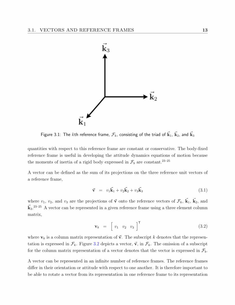
reference frame, F , is defined as a dextral, orthonormal triad.23–25 A triad is a set of three

unit vectors. The orthonormal and dextral adjectives restrict the vectors in the triad to be

mutually perpendicular and right-handed. Figure 3.1 is a diagram of the k reference frame,

Fk.

Two reference frames that are important in attitude dynamics are the inertial reference frame,

Fi, and the body-fixed reference frame, Fb. The inertial reference frame is a non-rotating

and non-accelerating reference frame. The inertial reference frame is useful because some

3.1. VECTORS AND REFERENCE FRAMES 13

Figure 3.1: The kth reference frame, Fk, consisting of the triad of ~k1, ~k2, and ~k3

quantities with respect to this reference frame are constant or conservative. The body-fixed

reference frame is useful in developing the attitude dynamics equations of motion because

the moments of inertia of a rigid body expressed in Fb are constant.23–25

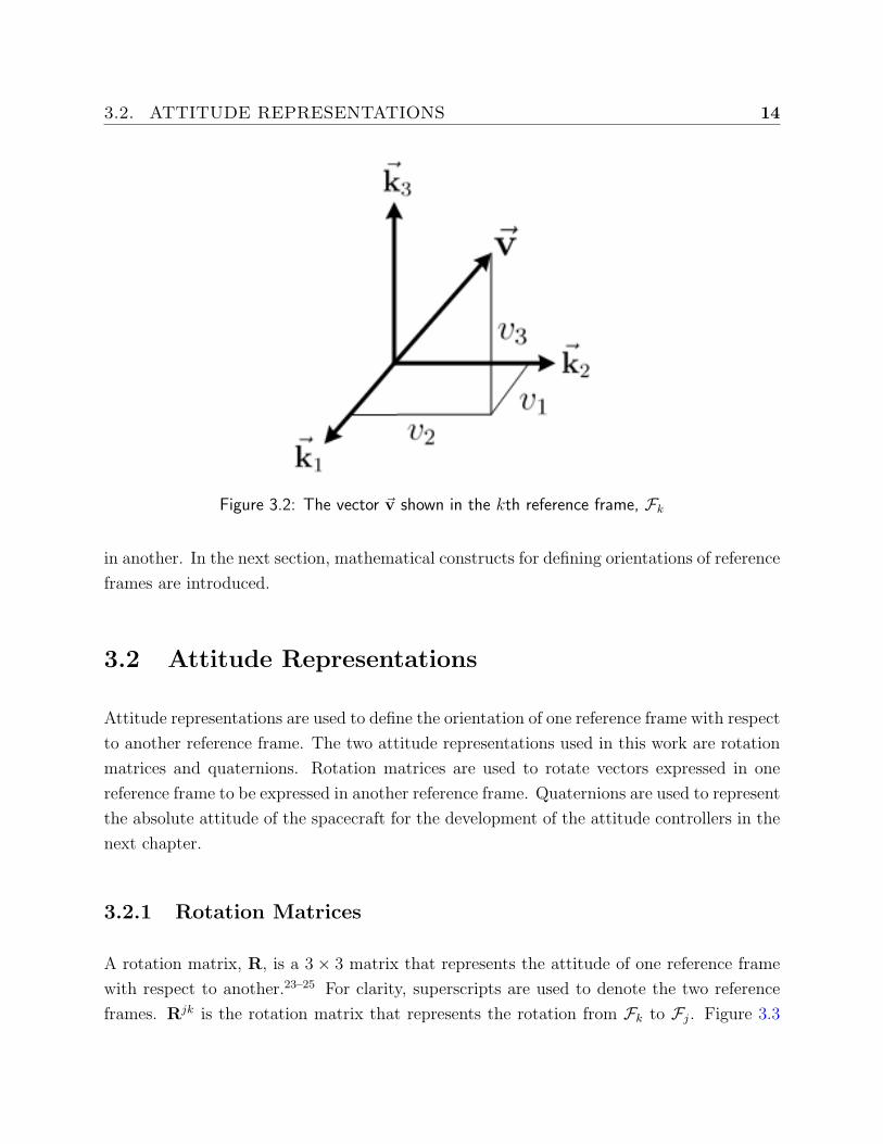
A vector can be defined as the sum of its projections on the three reference unit vectors of

a reference frame,

~v = v1~k1 + v2

~k2 + v3~k3 (3.1)

where v1, v2, and v3 are the projections of ~v onto the reference vectors of Fk, ~k1, ~k2, and~k3.

23–25 A vector can be represented in a given reference frame using a three element column

matrix,

vk =[

v1 v2 v3

]T(3.2)

where vk is a column matrix representation of ~v. The subscript k denotes that the represen-

tation is expressed in Fk. Figure 3.2 depicts a vector, ~v, in Fk. The omission of a subscript

for the column matrix representation of a vector denotes that the vector is expressed in Fb.

A vector can be represented in an infinite number of reference frames. The reference frames

differ in their orientation or attitude with respect to one another. It is therefore important to

be able to rotate a vector from its representation in one reference frame to its representation

3.2. ATTITUDE REPRESENTATIONS 14

Figure 3.2: The vector ~v shown in the kth reference frame, Fk

in another. In the next section, mathematical constructs for defining orientations of reference

frames are introduced.

3.2 Attitude Representations

Attitude representations are used to define the orientation of one reference frame with respect

to another reference frame. The two attitude representations used in this work are rotation

matrices and quaternions. Rotation matrices are used to rotate vectors expressed in one

reference frame to be expressed in another reference frame. Quaternions are used to represent

the absolute attitude of the spacecraft for the development of the attitude controllers in the

next chapter.

3.2.1 Rotation Matrices

A rotation matrix, R, is a 3 × 3 matrix that represents the attitude of one reference frame

with respect to another.23–25 For clarity, superscripts are used to denote the two reference

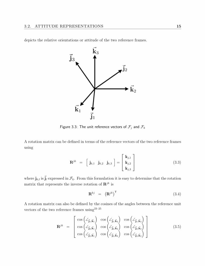
frames. Rjk is the rotation matrix that represents the rotation from Fk to Fj. Figure 3.3

3.2. ATTITUDE REPRESENTATIONS 15

depicts the relative orientations or attitude of the two reference frames.

Figure 3.3: The unit reference vectors of Fj and Fk

A rotation matrix can be defined in terms of the reference vectors of the two reference frames

using

Rjk =[

jk,1 jk,2 jk,3

]=

kj,1

kj,2

kj,3

(3.3)

where jk,l is~jl expressed in Fk. From this formulation it is easy to determine that the rotation

matrix that represents the inverse rotation of Rjk is

Rkj =(Rjk

)T(3.4)

A rotation matrix can also be defined by the cosines of the angles between the reference unit

vectors of the two reference frames using23–25

Rjk =

cos(∠~j1,~k1

)cos(∠~j1,~k2

)cos(∠~j1,~k3

)cos(∠~j2,~k1

)cos(∠~j2,~k2

)cos(∠~j2,~k3

)cos(∠~j3,~k1

)cos(∠~j3,~k2

)cos(∠~j3,~k3

) (3.5)

3.2. ATTITUDE REPRESENTATIONS 16

where ∠~jl,~kmis the angle between the lth reference vector of Fj and the mth reference vector

of Fk. The rotation matrix is also referred to as the direction cosine matrix, because of this

formulation, Eq. (3.5).

The rotation matrix attitude representation provides a simple method for adding succes-

sive rotations using matrix multiplication. The rotation matrix representing the successive

rotations of Rjk and Rlj is found using

Rlk = RljRjk (3.6)

The interior superscripts of the rotation matrices being multiplied are effectively cancelled.

Using Eqs. (3.4) and (3.6), the transpose of a rotation matrix is found to be equal to its

inverse,

Rjk(Rjk

)T= RjkRkj = Rjj = 1 (3.7)

where 1 is the identity matrix.

Rotation matrices are used to rotate a vector expressed in one reference frame to be expressed

in another reference frame. The vector ~v as expressed in Fj, vj, can be calculated using

vj = Rjkvk (3.8)

where vk is ~v as expressed in Fk.

Equations defining time development of the rotation matrix are required in the development

of the attitude tracking control laws. The first time derivative of the rotation matrix is

defined

Rjk = −ω×jkR

jk (3.9)

where ωjk is the angular velocity of Fj with respect to Fk expressed in Fj. The superscript

operator × denotes the skew-symmetric matrix given by

v =

v1

v2

v3

⇔ v× =

0 −v3 v2

v3 0 −v1

−v2 v1 0

(3.10)

Rotation matrices will be used in the development of the relative angular velocity vector

later in this chapter, and throughout the derivations of the attitude control laws presented

in the next two chapters.

3.2. ATTITUDE REPRESENTATIONS 17

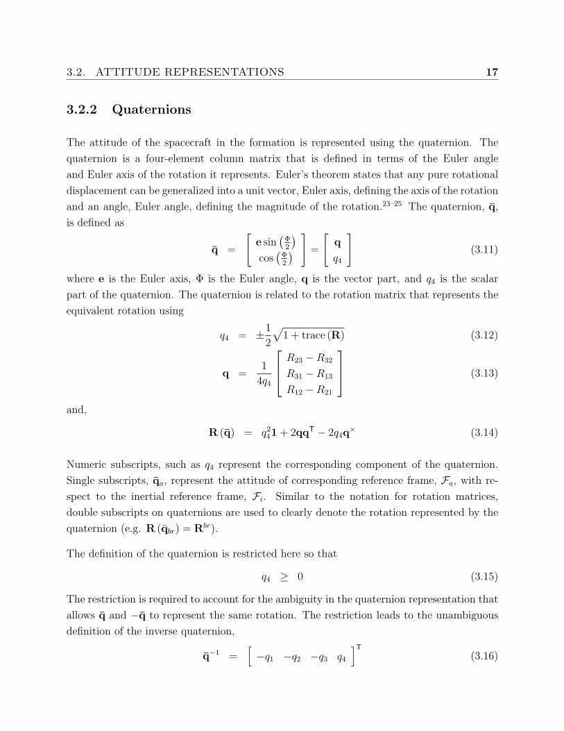
3.2.2 Quaternions

The attitude of the spacecraft in the formation is represented using the quaternion. The

quaternion is a four-element column matrix that is defined in terms of the Euler angle

and Euler axis of the rotation it represents. Euler’s theorem states that any pure rotational

displacement can be generalized into a unit vector, Euler axis, defining the axis of the rotation

and an angle, Euler angle, defining the magnitude of the rotation.23–25 The quaternion, q,

is defined as

q =

[e sin

(Φ2

)cos(

Φ2

) ] =

[q

q4

](3.11)

where e is the Euler axis, Φ is the Euler angle, q is the vector part, and q4 is the scalar

part of the quaternion. The quaternion is related to the rotation matrix that represents the

equivalent rotation using

q4 = ±1

2

√1 + trace (R) (3.12)

q =1

4q4

R23 −R32

R31 −R13

R12 −R21

(3.13)

and,

R (q) = q241 + 2qqT − 2q4q

× (3.14)

Numeric subscripts, such as q4 represent the corresponding component of the quaternion.

Single subscripts, qa, represent the attitude of corresponding reference frame, Fa, with re-

spect to the inertial reference frame, Fi. Similar to the notation for rotation matrices,

double subscripts on quaternions are used to clearly denote the rotation represented by the

quaternion (e.g. R (qbr) = Rbr).

The definition of the quaternion is restricted here so that

q4 ≥ 0 (3.15)

The restriction is required to account for the ambiguity in the quaternion representation that

allows q and −q to represent the same rotation. The restriction leads to the unambiguous

definition of the inverse quaternion,

q−1 =[−q1 −q2 −q3 q4

]T(3.16)

3.3. EQUATIONS OF MOTION 18

which represents the equal and opposite rotation represented by q. The inverse quaternion

has the property that

R (q)R(q−1)

= 1 (3.17)

Like the rotation matrix, the quaternion has a straight-forward method to mathematically

“add” successive rotations called quaternion multiplication. The quaternion that represents

the successive rotations of qb and qa is

qc = qa ⊗ qb (3.18)

where ⊗ is the operator for quaternion multiplication. The ⊗ operator is defined as

qc =

q4,a q3,a −q2,a q1,a

−q3,a q4,a q1,a q2,a

q2,a −q1,a q4,a q3,a

−q1,a −q2,a −q3,a q4,a

q1,b

q2,b

q3,b

q4,b

(3.19)

Quaternion multiplication is used extensively in the development of attitude error measures

later in this chapter.

The first time derivative of the quaternion is defined as

˙q =1

2ω ⊗ q (3.20)

where ω is defined

ω =[

ω 0]T

(3.21)

and ω is the angular velocity of the spacecraft. The omission of reference frame subscripts

denotes that ω is the angular velocity of Fb with respect to Fi expressed in Fb.

3.3 Equations of Motion

The individual spacecraft in the formation are modelled as rigid bodies. The angular mo-

mentum, h, of a spacecraft about its mass center with respect to inertial space is24

h = Iω (3.22)

3.4. ATTITUDE ERROR DYNAMICS 19

where I is the moment of inertia matrix of the spacecraft expressed in Fb. The moment of

inertia matrix of the spacecraft is constant, because of the rigid body assumption. The first

inertial time derivative of ~h in the body-fixed reference frame is

di

dt~h|b = h + ω×h (3.23)

= Iω + ω×Iω (3.24)

Euler’s equation states that24

d~h

dt= ~g (3.25)

where ~g is the external torque acting on the spacecraft. A useful form of the equations of

motion is found by combining Eqs. (3.24) and (3.25) and rearranging the terms to arrive at

Iω = g − ω×Iω (3.26)

Equation (3.26) is the form of the equations of motion used in the development of the

controllers presented in the next two chapters.

3.4 Attitude Error Dynamics

The development of the attitude controllers in the next chapter requires the definition of

attitude kinematic error variables. There are two measures of attitude error of an individual

spacecraft in a formation. The error measures are the station-keeping and formation-keeping

attitude state errors.

3.4.1 Station-Keeping Error

Station-keeping error is the attitude state error of an individual spacecraft with respect to

its absolute desired attitude. The station-keeping attitude error, δq, is defined

δq = q⊗ ˆq−1 (3.27)

where ˆq is the absolute desired attitude of the spacecraft formation. Using Eq. (3.20), the

first time derivative of δq is

δ ˙q =1

2δω ⊗ δq (3.28)

3.4. ATTITUDE ERROR DYNAMICS 20

The station-keeping angular velocity error, δω, is defined as

δω = ω −R (δq) ω (3.29)

where ω is the absolute desired angular velocity vector expressed in the absolute desired

reference frame. The first time derivative of δω is required in the development of the attitude

tracking controller. It is defined as

δω = ω −R (δq) ˙ω + δω×R (δq) ω (3.30)

where Eq. (3.9). The station-keeping error measure is used to determine the station-keeping

behavior control action.

3.4.2 Formation-Keeping Error

Formation-keeping error is the attitude state error of the individual spacecraft with respect

to the other spacecraft in the formation. The desired relative attitudes of the spacecraft in

the formation are assumed to be constant. The formation-keeping attitude error presents

a challenge if there are more than two spacecraft in the formation, because a physically

relevant average attitude measure does not exist. The equations developed in this section

deal with the error between two spacecraft in the formation. The attitude error between the

jth and kth spacecraft, qjk, is

qjk = qj ⊗ q−1k (3.31)

and can be defined in terms δqj and δqk,

qjk = δqj ⊗ ˆq−1j ⊗ (δqk ⊗ ˆq−1

k )−1

= δqj ⊗ ˆq−1j ⊗ ˆqk ⊗ δq−1

k

= δqj ⊗ δq−1k (3.32)

The time derivative of qij is

˙qjk =1

2ωjk ⊗ qjk (3.33)

where the relative angular velocity vector of the jth spacecraft with respect to the kth

spacecraft, ωjk, is defined as

ωjk = ωj −Rjkωk (3.34)

3.5. SUMMARY 21

and can be defined in terms δωj and δωk,

ωjk = δωj + R (δqj) ω −Rjk (δωk + R (δqk) ω)

= δωj −Rjkδωk (3.35)

The control action for the formation-keeping behavior is determined using the formation-

keeping error measures developed in this section.

3.5 Summary

A brief review of spacecraft attitude dynamics was given in this chapter. The important

basic concepts of vectors, reference frames, and attitude were introduced and defined. The

attitude representations used in this work were introduced and defined. The attitude kine-

matic and dynamic equations of motion were presented. Attitude error variables for the

spacecraft formation attitude control problem were developed. The concepts and equations

introduced in this chapter are used in the next chapter to develop control laws for a single,

rigid spacecraft.

22

Chapter 4

Spacecraft Attitude Control

Nonlinear techniques for the analysis of the stability characteristics of a nonlinear controller

are introduced in this chapter. Two attitude controllers for a single spacecraft are analyzed

using these techniques. The analytic stability and convergence results are reinforced using

numeric simulation results. The attitude controllers are extended in the next chapter to

develop coordinated attitude controllers for a spacecraft formation.

4.1 Lyapunov Stability Theory

The goal of a controller is to determine the control actions required to ensure that the desired

state or trajectory of the system is an asymptotically stable equilibrium point of the system.

Techniques for the analysis of the stability of equilibrium points of autonomous systems

are introduced in this section. A system whose dynamics are independent of time is an

autonomous system. A general state-space representation of an autonomous system is

x = f (x) (4.1)

An equilibrium point of the system, x, satisfies the equation,

f (x) = 0 (4.2)

An equilibrium point is stable, in the sense of Lyapunov, if a solution that begins near the

equilibrium point will stay near the equilibrium point for all time, otherwise the equilibrium

4.1. LYAPUNOV STABILITY THEORY 23

point is unstable.26 A formal mathematical definition for the stability of an equilibrium

point is presented in Definition 1.

Definition 1 (Stability of an Equilibrium Point26) An equilibrium point, x, of the sys-

tem described by Eq. (4.1) is stable if and only if

‖x− x(0)‖ < δ ⇒ ‖x− x(t)‖ < ε, ∀ t ≥ 0

where δ and ε are positive constants. 2

An equilibrium point is asymptotically stable, if a solution that begins near the equilibrium

point tends toward the equilibrium point as time progresses. Definition 2 presents a formal

mathematical definition for the asymptotic stability of an equilibrium point.

Definition 2 (Asymptotic Stability of an Equilibrium Point26) An equilibrium point,

x, of the system described by Eq. (4.1) is asymptotically stable if and only if

‖x− x(0)‖ < δ ⇒ lim ‖x− x(t)‖ = 0, ∀ t ≥ 0

where δ is a positive constant. 2

Lyapunov stability theory is useful in the analysis of nonlinear systems. Analytic solutions

to nonlinear systems are often difficult to obtain. Lyapunov stability theory allows for

the stability analysis of equilibrium points without determining analytic solutions to the

nonlinear system. In Lyapunov stability theory, a scalar-valued, vector function of the system

states, called a Lyapunov function, V , is used to determine the stability characteristics of

the system. The requirements on the Lyapunov function to guarantee local stability and

local asymptotic stability of the system are presented in Theorem 1.

Theorem 1 (Lyapunov Stability Theorem26) Let x = x be an equilibrium point for

the system described by Eq. (4.1). Let V be a continuously differentiable function on a

neighborhood D of x that maps Rn on to R, such that

V (x) = 0 and V (x) > 0 in D − {x}

V (x) ≤ 0 in D

Then, x = x is a stable equilibrium point of the system. Moreover, if

V (x) < 0 in D − {x}

Then, x = x is an asymptotically stable equilibrium point of the system. 2

4.1. LYAPUNOV STABILITY THEORY 24

Global asymptotic stability of the system can be proven if the additional requirement of

a radially-unbounded Lyapunov function is added to the asymptotic stability requirements

presented in Theorem 1. Theorem 2 presents the formal mathematic requirements to prove

global asymptotic stability of the system.

Theorem 2 (Barbashin-Krasovskii Theorem26) Let x = x be an equilibrium point of

the system described by Eq. (4.1). Let V be a continuously differentiable function of x that

maps Rn on to R, such that

V (x) = 0 and V (x) > 0, ∀ x 6= x

and, if

‖x‖ → ∞⇒ V (x) →∞

V (x) < 0, ∀ x 6= 0

Then, x = x is a globally asymptotically stable equilibrium point. 2

The analysis of the stability of spacecraft attitude controllers often leads to a negative-semi-

definite V . Therefore, only global stability can be proven using the theorems and definitions

already given in the section. LaSalle’s invariance principle provides a method to prove that

the controller is asymptotically stable by investigating the solutions for which V = 0. A

formal statement of the invariance principle is presented in Theorem 3.

Theorem 3 (LaSalle’s Invariance Principle26) Let x = x be an equilibrium point of the

system described by Eq. (4.1). Let V be a continuously-differentiable, radially-unbounded,

positive-definite function of x that maps Rn on to R, such that V ≤ 0 for x ∈ Rn. Let S be

a subset of Rn where V = 0 for x ∈ S, and suppose that no solution can stay forever in S

other than the solution at x. Then, the equilibrium point is globally asymptotically stable. 2

Stability definitions, Lyapunov stability theorems, and LaSalle’s invariance principle were

presented in this section. These definitions and theorems are used to prove the global

asymptotic stability of the individual spacecraft attitude controllers presented in the next

two sections.

4.2. QUATERNION-BASED ATTITUDE CONTROLLER 25

4.2 Quaternion-Based Attitude Controller

A linear attitude control law for a single, rigid spacecraft using external control torques is

g = −kpq− kdω (4.3)

This control law was first introduced by Mortensen27 and was later included in a survey of

attitude representations for use in attitude control by Tsiotras.28 The control law is proven

to guarantee the attitude stability of a rigid body using the candidate Lyapunov function,

V =1

2ωTIω + kpq

Tq + (1− q4)2 (4.4)

Equation (4.4) defines a positive definite function that is radially unbounded. The first time

derivative of V is

V = ωTIω + 2kpqTq− 2 (1− q4) q4 (4.5)

Using Eq. (3.20), V simplifies to

V = ωTIω + kpωTq (4.6)

= ωT (Iω + kpq) (4.7)

The closed-loop attitude dynamics of the spacecraft, Eqs. (3.26) and (4.3), are used to arrive

at

V = −kdωTω (4.8)

Equation (4.4) is a positive-definite, radially-unbounded function, whose first time derivative

is negative semi-definite. Thus, V is a Lyapunov function, and the attitude of the spacecraft

is globally stable, because the function satisfies the requirements of Theorem 1.

The convergence of the spacecraft’s attitude is proven using an invariance argument. Equa-

tion (4.8) guarantees that

limt→∞

ω = 0 (4.9)

The closed-loop attitude dynamics of the spacecraft are

Iω = −kpq− kdω − ω×Iω (4.10)

4.2. QUATERNION-BASED ATTITUDE CONTROLLER 26

Applying Eq. (4.9) to Eq. (4.10)

q = 0 (4.11)

Therefore,

limt→∞

q = 0 (4.12)

and the attitude of the spacecraft converges to the desired attitude.

4.2.1 Simulation Results

The stability analysis is reinforced by numeric simulation of a spacecraft using the quaternion-

based attitude control law, Eq. (4.3). The moment of inertia matrix, I, of the simulated

spacecraft is

I =

2 0 0

0 3 0

0 0 4

kg ·m2 (4.13)

The control gains used for the simulation are

kp = 3 (4.14)

kd = 5 (4.15)

The control gains are chosen to allow the spacecraft to converge to the desired attitude

in a reasonable time to prevent long simulation times. The ratio of the proportional and

derivative gains was chosen to prevent severe oscillations of the spacecraft. Because, the

stability and convergence results presented in the previous section are independent of the

control gains, the actual values chosen for the gains are not critical. The attitude and angular

velocity of the spacecraft are initialized to

q0 =[

0.0559 0.3652 −0.0260 0.9289]T

(4.16)

ω0 =[

0.0123 −0.0123 0]T

rad/s (4.17)

The spacecraft is commanded to a desired attitude of

ˆq =[

0 0 0 1]T

(4.18)

4.2. QUATERNION-BASED ATTITUDE CONTROLLER 27

which corresponds to with the inertial reference frame.

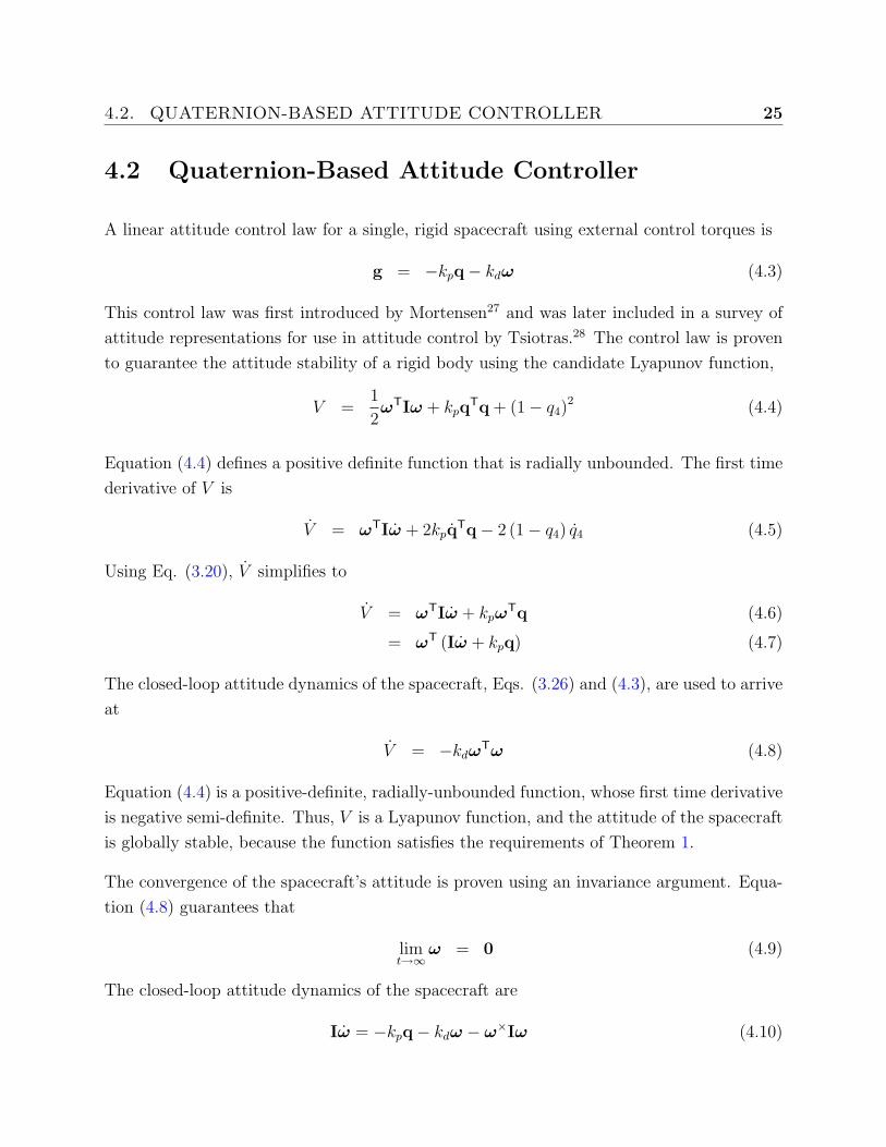
The results of the simulation are presented in Figures 4.1, 4.2, and 4.3. Figure 4.1 contains

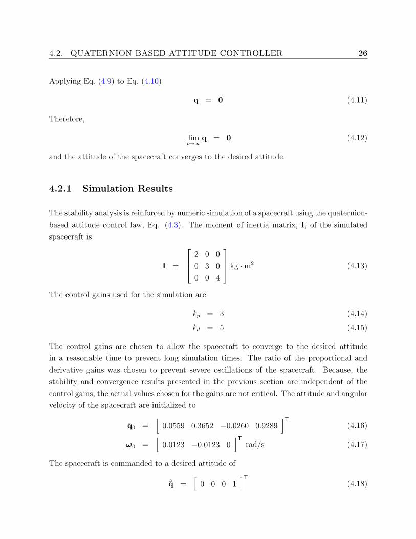
the angular error of the spacecraft, in degrees, throughout the simulation. Figure 4.2 contains

plots of the angular rate error of the spacecraft in o/s. In both figures the upper plot displays

the results using a linear scale and the lower plot uses a log scale on the ordinate axis. The

semi-log plots are shown to better depict the features of the curves. The plots in both figures

show that the spacecraft’s attitude converges to the desired attitude. The angular error curve

on the semi-log plot stops approximately 85 seconds into the simulation, because the error

reaches “machine zero.” The angular rate error decreases through the first 135 seconds of

the simulation. After this point in the simulation the angular rate error has reached the

integration tolerance limit, 10−8.

Figure 4.1: Angular error of the spacecraft during the simulation

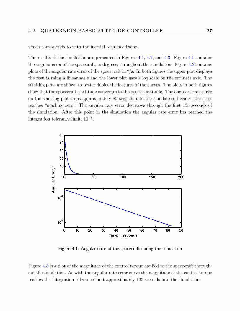
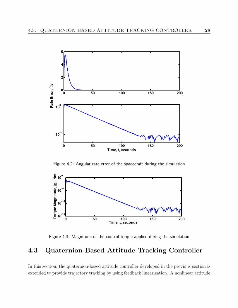
Figure 4.3 is a plot of the magnitude of the control torque applied to the spacecraft through-

out the simulation. As with the angular rate error curve the magnitude of the control torque

reaches the integration tolerance limit approximately 135 seconds into the simulation.

4.3. QUATERNION-BASED ATTITUDE TRACKING CONTROLLER 28

Figure 4.2: Angular rate error of the spacecraft during the simulation

Figure 4.3: Magnitude of the control torque applied during the simulation

4.3 Quaternion-Based Attitude Tracking Controller

In this section, the quaternion-based attitude controller developed in the previous section is

extended to provide trajectory tracking by using feedback linearization. A nonlinear attitude

4.3. QUATERNION-BASED ATTITUDE TRACKING CONTROLLER 29

tracking control law for a single, rigid spacecraft is

g = ω×Iω + I(R (δq) ˙ω + δω×R (δq) ω

)− kpδq− kdδω (4.19)

Equation (4.19) is an extended version of the control law presented in Eq. (4.3). The addition

of the first two nonlinear terms in Eq. (4.19) allows the spacecraft to track a given reference

attitude trajectory. The first term cancels out the nonlinear gyroscopic torque term in the

rigid body equations of motion. The second term represents the control action required to

follow the desired attitude trajectory.

The candidate Lyapunov function,

V =1

2δωTIδω + kpδq

Tδq + (1− δq4)2 (4.20)

is used to prove that the control law globally stabilizes the attitude of the spacecraft. Equa-

tion (4.20) is radially-unbounded and positive-definite. The first time derivative of the

candidate Lyapunov function is

V = δωTIδω + 2kpδqTδq− 2 (1− δq4) δq4 (4.21)

Using Eq. (3.20), V simplifies to

V = δωTIδω + kpδωTδq (4.22)

= δωT (Iδω + kpδq) (4.23)

The equation is further simplified using the closed-loop attitude dynamics of the spacecraft,

V = −kdδωTδω (4.24)

which is negative semi-definite. The candidate Lyapunov function, Eq. (4.19), is thus proven

to be a true Lyapunov function. All of the conditions of Theorem 1 are satisfied, and there-

fore the quaternion-based attitude tracking control law globally stabilizes the spacecraft’s

attitude. The attitude tracking control law, Eq. (4.19), globally stabilizes the attitude of the

spacecraft.

An invariance argument is used to prove that the attitude tracking control law guarantees

global convergence of the spacecraft’s attitude to the desired attitude reference trajectory.

Equation (4.24) requires

limt→∞

δω = 0 (4.25)

4.3. QUATERNION-BASED ATTITUDE TRACKING CONTROLLER 30

The closed-loop attitude dynamics of the spacecraft are

Iδω = −kpδq− kdδω (4.26)

Applying Eq. (4.25) to Eq. (4.26)

δq = 0 (4.27)

Therefore,

limt→∞

δq = 0 (4.28)

The spacecraft’s attitude converges to the desired attitude reference trajectory.

4.3.1 Simulation Results

Numeric simulation of a single spacecraft is performed to validate the analytic stability

analysis presented for the quaternion-based attitude tracking controller, Eq. (4.19), in the

previous section. The proportional and derivative control gains and the moment of inertia

matrix used in the simulation are the same as those used in the quaternion-based attitude

controller simulation. The attitude and angular velocity of the spacecraft are initialized to

q0 =[

0.1339 0.0529 0.0734 0.9869]T

(4.29)

ω0 =[

0.0011 0.0745 0.0548]T

rad/s (4.30)

The spacecraft is commanded to track the attitude trajectory of a reference spacecraft that

is performing a 90o slew maneuver about its ~b2 axis in 90 seconds. The initial attitude of

the reference spacecraft is set to

ˆq0 =[

0 0 0 1]T

(4.31)

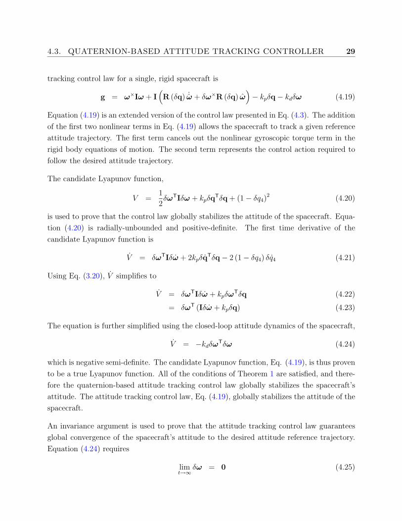
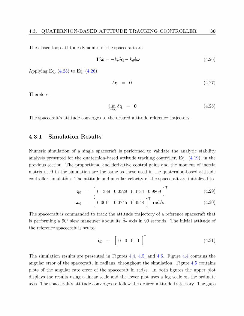
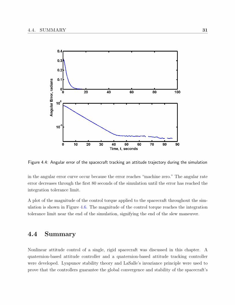
The simulation results are presented in Figures 4.4, 4.5, and 4.6. Figure 4.4 contains the

angular error of the spacecraft, in radians, throughout the simulation. Figure 4.5 contains

plots of the angular rate error of the spacecraft in rad/s. In both figures the upper plot

displays the results using a linear scale and the lower plot uses a log scale on the ordinate

axis. The spacecraft’s attitude converges to follow the desired attitude trajectory. The gaps

4.4. SUMMARY 31

Figure 4.4: Angular error of the spacecraft tracking an attitude trajectory during the simulation

in the angular error curve occur because the error reaches “machine zero.” The angular rate

error decreases through the first 80 seconds of the simulation until the error has reached the

integration tolerance limit.

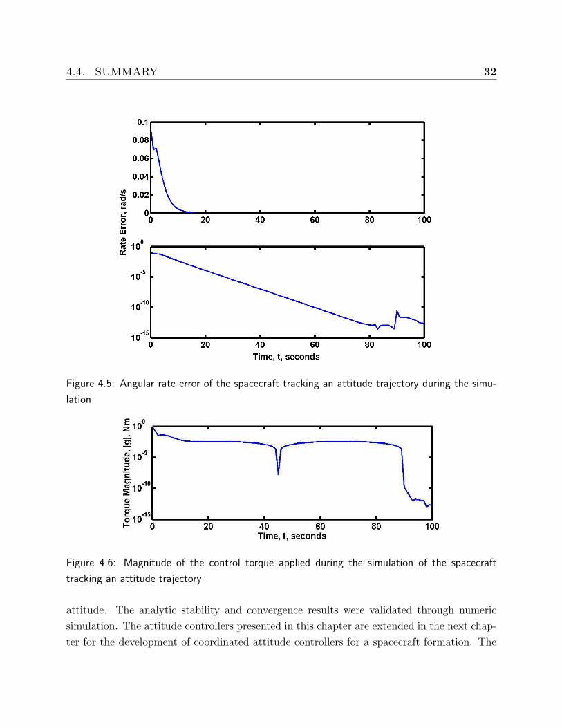
A plot of the magnitude of the control torque applied to the spacecraft throughout the sim-

ulation is shown in Figure 4.6. The magnitude of the control torque reaches the integration

tolerance limit near the end of the simulation, signifying the end of the slew maneuver.

4.4 Summary

Nonlinear attitude control of a single, rigid spacecraft was discussed in this chapter. A

quaternion-based attitude controller and a quaternion-based attitude tracking controller

were developed. Lyapunov stability theory and LaSalle’s invariance principle were used to

prove that the controllers guarantee the global convergence and stability of the spacecraft’s

4.4. SUMMARY 32

Figure 4.5: Angular rate error of the spacecraft tracking an attitude trajectory during the simu-

lation

Figure 4.6: Magnitude of the control torque applied during the simulation of the spacecraft

tracking an attitude trajectory

attitude. The analytic stability and convergence results were validated through numeric

simulation. The attitude controllers presented in this chapter are extended in the next chap-

ter for the development of coordinated attitude controllers for a spacecraft formation. The

4.4. SUMMARY 33

analytic stability and convergence analysis methods introduced in this chapter are used to

analyze the coordinated attitude controllers.

34

Chapter 5

Spacecraft Formation Attitude

Control

The deficiencies in the literature discussed in Chapter 2 are resolved in this chapter. A class

of decentralized attitude control laws is introduced. The control laws extend the quaternion-

based attitude control law and the quaternion-based attitude tracking control law developed

in the previous chapter. The analytical methods presented in Chapter 4 are used to prove

that the class of control laws guarantee global stability and convergence of the spacecraft

formation.

5.1 Problem Statement

The problem is formally defined before introducing the class of attitude control laws. The

coordination of the attitude control systems of a spacecraft formation is considered. First,

the approach used in solving the problem is discussed. Then the assumptions used in the

development and analysis of the class of control laws are stated. Finally, the scope of the

research is defined.

5.1. PROBLEM STATEMENT 35

5.1.1 Approach

The two control methodology challenges presented by spacecraft formation attitude control

are coordination and conflicting desired control behaviors.

The spacecraft formation is treated as a distributed system. The control systems of the

individual spacecraft are coordinated through the communication of attitude state data. A

decentralized coordination architecture is used, because of the system architecture benefits

and the lack of prior proper investigation of this approach. Systems that use decentralized

control architectures are fault-tolerant, and simple to upgrade and repair. Decentralized

architectures are fault-tolerant because the resulting system does not have a single point of

failure. Failure of a local subsystem does not lead to the destabilization of the entire system.18

Repairs to the formation can simply be performed by replacing malfunctioning spacecraft.

Upgrades can take the form of replacing obsolete spacecraft with a more advanced version, or

by simply adding spacecraft to the formation. The drawback of decentralized controllers is

the difficulty in producing analytic convergence proofs. The problem of analytic convergence

proofs for decentralized controllers is discussed and resolved in this chapter.

Coordination is also accomplished through the use of the virtual structure method. The

virtual structure method models the formation as one large, rigid spacecraft. The attitude

of the virtual structure is the desired absolute attitude of the formation. Each spacecraft is

able to determine its desired absolute attitude, because each spacecraft knows the attitude

trajectory of the virtual structure and its constant attitude offset from that attitude. The

addition of these rotations is the desired absolute attitude of the spacecraft.

An attitude control system of a spacecraft in a formation has two desired control behaviors:

station-keeping and formation-keeping. The two behaviors often conflict due to the inevitable

tracking errors of the spacecraft. Behavior-based control is used to reconcile the conflict

and concurrently satisfy the desired control behaviors. The attitude control laws for the

spacecraft in the formation are extended versions of the single spacecraft attitude control

laws presented in the previous chapter. The single spacecraft attitude control laws represent

the station-keeping behavior control terms. The formation-keeping behavior is satisfied by

adding terms involving the relative attitude states of the spacecraft in the formation. The

resultant control action is a compromise between the station-keeping and formation-keeping

desired control behaviors.

5.1. PROBLEM STATEMENT 36

Lyapunov stability theory is used to analyze the stability characteristics of the coordinated

attitude control laws. A spacecraft formation is a special case of a distributed system where

the subsystems are similar with respect to the form of their equations of motion. Therefore,

it is prudent to separate the system’s Lyapunov function into component Lyapunov functions

for each subsystem. A component Lyapunov function incorporates all information about a

specific subsystem (e.g. individual spacecraft). The Lyapunov function for the global system,

the composite Lyapunov function, is the sum of the component Lyapunov functions. The

composite Lyapunov function can be used to investigate the stability and convergence char-

acteristics of the global system using Lyapunov stability theory. The stability characteristics

of the coordinated attitude control laws are investigated using component and composite

Lyapunov functions.26

5.1.2 Assumptions

Several assumptions relating to the nature of the spacecraft formation and the individual

spacecraft are made to simplify the development and analysis of the class of decentralized

attitude control laws. The spacecraft formation is assumed to have a rigid configuration

and to be free-flying. The rigid configuration constraint requires that the desired relative

attitudes of the spacecraft in the formation be constant. Therefore, the desired relative

angular velocity of the spacecraft in the formation is identically zero. A free-flying spacecraft

formation has no physical connections between the spacecraft in the formation, such as

tethers or booms. The individual spacecraft interact only through the communication of

state information between the spacecraft.

The spacecraft are assumed to be rigid bodies that use external torque actuation for atti-

tude control. The rigid body assumption simplifies the attitude dynamics of the spacecraft.

Although external torque actuation is used in developing the coordinated control laws, ex-

tending the results to use internal torque actuation is a straight-forward matter. The internal

torque actuation extension is not included because there are no important or significant dif-

ferences in that development.

5.2. THE DECENTRALIZED COORDINATED ATTITUDE CONTROLLER37

5.1.3 Scope of Research

The focus of this research is the development of a decentralized coordinated attitude control

law. An emphasis is placed on proving analytically that the decentralized controller guaran-

tees a global asymptotically stable system. The effects of the control law parameters, such

as control gains and coordination architecture are also investigated.

An in-depth analysis of the effects of communication disturbances between spacecraft and

parameter uncertainties on the performance and stability of the spacecraft formation is not

within the scope of this work. The communication between spacecraft is considered perfect.

Each spacecraft knows its current attitude and the current attitudes of the spacecraft that are

communicating with it at all times. Communication interrupts or failures are not considered.

Bandwidth limitations on communication are also not considered. Uncertainty effects are not

included in the scope of this research. The controllers are assumed to have perfect knowledge

of the spacecraft parameters (e.g. moments of inertia). Control actuation is assumed to be

perfect.

5.2 The Decentralized Coordinated Attitude Controller

As discussed in the Approach section, a behavior-based control methodology is used to

develop the class of decentralized attitude control laws. The first step in behavior-based

control is the determination of the control actions for the desired control behaviors.

5.2.1 Desired Behavior Control Actions

The two desired behaviors for a spacecraft formation are station-keeping and formation-

keeping. The control action for the attitude-tracking station-keeping behavior for the jth

spacecraft, gsj , is calculated using

gsj = ω×

j Ijωj + Ij

(R (δqj) ˙ω − δω×

j R (δqj) ω)− kpj

δqj − kdjδωj (5.1)

If the desired attitude of the formation is constant, then the station-keeping control action

can be simplified to

gsj = −kpj

qj − kdjωj (5.2)

5.2. THE DECENTRALIZED COORDINATED ATTITUDE CONTROLLER38

Equations (5.1) and (5.2) are identical to the single spacecraft attitude control law, Eq. (4.3),

and the single, spacecraft attitude tracking control law, Eq. (4.19), presented in Chapter 4.

The station-keeping control action drives the absolute attitude state error to zero.

The control action for the formation-keeping behavior for the jth spacecraft, gfj , is calculated

using

gfj = −

n∑k=1

ρpjkqjk −

n∑k=1

ρdjkωjk (5.3)

where ρpjk is the proportional formation-keeping behavior weighting, ρd

jk is the derivative

formation-keeping behavior weighting, and n is the number of spacecraft in the formation.

The control action for the formation-keeping behavior drives the relative attitude state error,

qjk and ωjk, between connected spacecraft to zero. The proportional behavior weighting

factor, ρpjk, determines the importance of the relative alignment of the jth and the kth

spacecraft in the formation. The derivative behavior weighting factor, ρdjk, determines the

importance of the jth and the kth spacecraft in the formation maintaining the same angular

rate. The value of ρpjk is restricted so that

ρpjk ≥ 0 and

n∑k=1

ρpjk < kpj

∀ j = 1, 2, ..., n (5.4)

and the value of ρdjk is restricted so that

ρdjk ≥ 0 (5.5)

These restrictions are necessary for the convergence proof presented later in this chapter.

Both the proportional and derivative behavior weights are further restricted by

ρjk = ρkj (5.6)

The second restriction, Eq. (5.6), requires that the importance of the relative alignment and

angular rate of the jth and kth spacecraft be the same for the jth spacecraft and the kth

spacecraft.

5.2.2 The Control Law

The decentralized attitude control law is determined by summing the control actions for

the station-keeping and formation-keeping behaviors. The resulting control law for the jth

5.3. COORDINATION ARCHITECTURES 39

spacecraft, gj, is

gj = gsj + gf

j (5.7)

= ω×j Ijωj + Ij

(R (δqj) ˙ω − δω×

j R (δqj) ω)− kpδqj − kdδωj

−n∑

k=1

ρpjkqjk −

n∑k=1

ρdjkωjk

The control law, Eq. (5.7), is an extension of the single spacecraft quaternion-based attitude

tracking control law presented in Chapter 4. The control law is extended in recognition

that the spacecraft is part of a larger system, the spacecraft formation. The two summation

terms appended to the end of the equation represent the modification. These terms enforce

an interconnection between the spacecraft in the formation. Throughout the rest of this

work, a non-zero ρjk is referred to as a connection between spacecraft. The magnitude of ρjk

represents the strength of the connection between the spacecraft. This terminology is used

to more clearly indicate the interdependency of the spacecraft in the formation.

5.3 Coordination Architectures

Equation (5.7) represents a class of decentralized control laws that differ by the coordination

architecture used by the spacecraft formation. The choice of the formation-keeping weighting

factors, ρjk, determine the coordination architecture used. Variants of coordination archi-

tectures can be created by altering the number of connections between spacecraft and the

strength of the connections.

Four different coordination architectures for a six-spacecraft formation are presented in Fig-

ure 5.1. The circles represent the individual spacecraft. Connections between the spacecraft

are denoted by bi-directional arrows. The coordination architectures in Figure 5.1 differ in

the number of connections per spacecraft, c, used. Diagram A depicts an architecture with

no connection between the spacecraft. In this architecture the spacecraft act independently

as if they were not part of a formation. Diagram B shows a coordination architecture with

two connections per spacecraft. This type of coordination architecture is used by the velocity

feedback controller presented in Lawton and Beard14 and the “coupled-dynamics controller”

presented in Lawton, Beard and Hadaegh.10 The authors term the two-connection archi-

tecture the “ring” coordination architecture. Diagram C shows an architecture with three

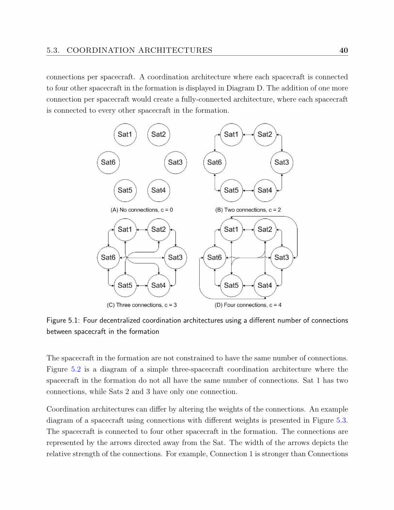
5.3. COORDINATION ARCHITECTURES 40

connections per spacecraft. A coordination architecture where each spacecraft is connected

to four other spacecraft in the formation is displayed in Diagram D. The addition of one more

connection per spacecraft would create a fully-connected architecture, where each spacecraft

is connected to every other spacecraft in the formation.

Figure 5.1: Four decentralized coordination architectures using a different number of connections

between spacecraft in the formation

The spacecraft in the formation are not constrained to have the same number of connections.

Figure 5.2 is a diagram of a simple three-spacecraft coordination architecture where the

spacecraft in the formation do not all have the same number of connections. Sat 1 has two

connections, while Sats 2 and 3 have only one connection.

Coordination architectures can differ by altering the weights of the connections. An example

diagram of a spacecraft using connections with different weights is presented in Figure 5.3.

The spacecraft is connected to four other spacecraft in the formation. The connections are

represented by the arrows directed away from the Sat. The width of the arrows depicts the

relative strength of the connections. For example, Connection 1 is stronger than Connections

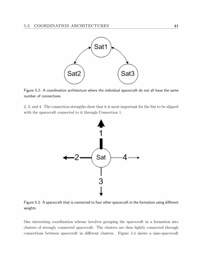
5.3. COORDINATION ARCHITECTURES 41

Figure 5.2: A coordination architecture where the individual spacecraft do not all have the same

number of connections

2, 3, and 4. The connection strengths show that it is most important for the Sat to be aligned

with the spacecraft connected to it through Connection 1.

Figure 5.3: A spacecraft that is connected to four other spacecraft in the formation using different

weights

One interesting coordination scheme involves grouping the spacecraft in a formation into

clusters of strongly connected spacecraft. The clusters are then lightly connected through

connections between spacecraft in different clusters. Figure 5.4 shows a nine-spacecraft

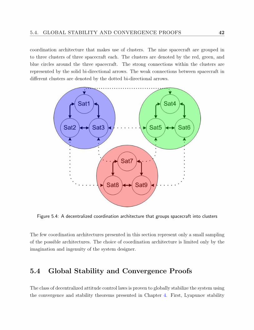
5.4. GLOBAL STABILITY AND CONVERGENCE PROOFS 42

coordination architecture that makes use of clusters. The nine spacecraft are grouped in

to three clusters of three spacecraft each. The clusters are denoted by the red, green, and

blue circles around the three spacecraft. The strong connections within the clusters are

represented by the solid bi-directional arrows. The weak connections between spacecraft in

different clusters are denoted by the dotted bi-directional arrows.

Figure 5.4: A decentralized coordination architecture that groups spacecraft into clusters

The few coordination architectures presented in this section represent only a small sampling

of the possible architectures. The choice of coordination architecture is limited only by the

imagination and ingenuity of the system designer.

5.4 Global Stability and Convergence Proofs

The class of decentralized attitude control laws is proven to globally stabilize the system using

the convergence and stability theorems presented in Chapter 4. First, Lyapunov stability

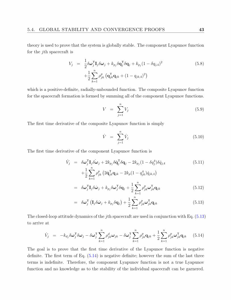
5.4. GLOBAL STABILITY AND CONVERGENCE PROOFS 43

theory is used to prove that the system is globally stable. The component Lyapunov function

for the jth spacecraft is

Vj =1

2δωT

j Ijδωj + kpjδqT

j δqj + kpj(1− δqj,4)

2 (5.8)

+1

2

n∑k=1

ρpjk

(qT

jkqjk + (1− qjk,4)2)

which is a positive-definite, radially-unbounded function. The composite Lyapunov function

for the spacecraft formation is formed by summing all of the component Lyapunov functions.

V =n∑

j=1

Vj (5.9)

The first time derivative of the composite Lyapunov function is simply

V =n∑

j=1

Vj (5.10)

The first time derivative of the component Lyapunov function is

Vj = δωTj Ij

˙δωj + 2kpjδqT

j δqj − 2kpj(1− δq4

j )δqj,4 (5.11)

+1

2

n∑k=1

ρpjk

(2qT

jkqjk − 2kp(1− q4jk)qjk,4

)= δωT

j Ijδωj + kpjδωT

j δqj +1

2

n∑k=1

ρpjkω

Tjkqjk (5.12)

= δωTj

(Ijδωj + kpj

δqj

)+

1

2

n∑k=1

ρpjkω

Tjkqjk (5.13)

The closed-loop attitude dynamics of the jth spacecraft are used in conjunction with Eq. (5.13)

to arrive at

Vj = −kdjδωT

j δωj − δωTj

n∑k=1

ρdjkωjk − δωT

j

n∑k=1

ρpjkqjk +

1

2

n∑k=1

ρpjkω

Tjkqjk (5.14)

The goal is to prove that the first time derivative of the Lyapunov function is negative

definite. The first term of Eq. (5.14) is negative definite; however the sum of the last three

terms is indefinite. Therefore, the component Lyapunov function is not a true Lyapunov

function and no knowledge as to the stability of the individual spacecraft can be garnered.

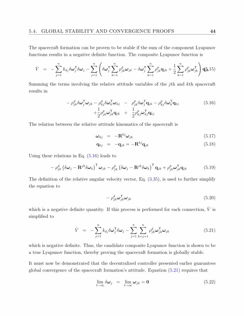
5.4. GLOBAL STABILITY AND CONVERGENCE PROOFS 44

The spacecraft formation can be proven to be stable if the sum of the component Lyapunov

functions results in a negative definite function. The composite Lyapunov function is

V = −n∑

j=1

kdjδωT

j δωj −n∑

j=1

(δωT

j

n∑k=1

ρdjkωjk − δωT

j

n∑k=1

ρpjkqjk +

1

2

n∑k=1

ρpjkω

Tjk

)qjk(5.15)

Summing the terms involving the relative attitude variables of the jth and kth spacecraft

results in

− ρdjkδω

Tj ωjk − ρd

kjδωTk ωkj − ρp

jkδωTj qjk − ρp

kjδωTk qkj (5.16)

+1

2ρp

jkωTjkqjk +

1

2ρp

kjωTkjqkj

The relation between the relative attitude kinematics of the spacecraft is

ωkj = −Rkjωjk (5.17)

qkj = −qjk = −Rkjqjk (5.18)

Using these relations in Eq. (5.16) leads to

− ρdjk

(δωj −Rjkδωk

)Tωjk − ρp

jk

(δωj −Rjkδωk

)Tqjk + ρp

jkωTjkqjk (5.19)

The definition of the relative angular velocity vector, Eq. (3.35), is used to further simplify

the equation to

− ρdjkω

Tjkωjk (5.20)

which is a negative definite quantity. If this process is performed for each connection, V is

simplified to

V = −n∑

j=1

kdjδωT

j δωj −n∑

j=1

n∑k=j+1

ρdjkω

Tjkωjk (5.21)

which is negative definite. Thus, the candidate composite Lyapunov function is shown to be

a true Lyapunov function, thereby proving the spacecraft formation is globally stable.

It must now be demonstrated that the decentralized controller presented earlier guarantees

global convergence of the spacecraft formation’s attitude. Equation (5.21) requires that

limt→∞

δωj = limt→∞

ωjk = 0 (5.22)

5.4. GLOBAL STABILITY AND CONVERGENCE PROOFS 45

If this result is applied to the closed-loop dynamics of the system, the result is a system of

n equations of the form,

kpjδqj +

n∑k=1

ρpjkqjk = 0 (5.23)

Using the definition of qjk, Eq. (5.23) can be re-written as

0 = kpjδqj +

n∑k=1

ρpjk

((δq×k + δqk,41

)δqj − δqj,4δqk

)(5.24)

= kpjδqj +

((n∑

k=1

ρpjkδqk

)×+

n∑k=1

ρpjkδqk,41

)δqj − δqj,4

n∑k=1

ρpjkδqk (5.25)

which can be written in the convenient form,

δq×j

n∑k=1

ρpjkδqk =

(kpj

+n∑

k=1

ρpjkδqk,4

)δqj − δqkj,4

n∑k=1

ρpjkδqk (5.26)

The right side of Eq. (5.26) is a linear combination of the vectors, δqj and∑n

k=1 ρpjkδqk, and

the left side of the equation is the cross product of the same two vectors. The equality is

only satisfied if

δq×j

n∑k=1

ρpjkδqk = 0 (5.27)

Therefore, Eq. (5.26) simplifies to(kpj

+n∑

k=1

ρpjkδqk,4

)δqj − δqj,4

n∑k=1

ρpjkδqk = 0 (5.28)

which is solved for δqj

δqj =δqj,4

kp +∑n

k=1 ρpjkδqk,4

n∑k=1

ρpjkδqk (5.29)

The set of n equations that result can be represented in matrix form as

Q = MQ (5.30)

where the 3n× 1 column vector Q

Q =[

δqT1 · · · δqT

n

]T(5.31)

5.4. GLOBAL STABILITY AND CONVERGENCE PROOFS 46

The 3n× 3n matrix M is defined

mjk = κjρpjk (5.32)

where

κj =δqj,4

kpj+∑n

k=1 ρpjkδqk,4

(5.33)

The upper limit of the magnitude of κj is

κj ≤ 1

kpj

(5.34)

This value becomes important later in the proof. Re-writing Eq. (5.30) in homogeneous form

results in

(1−M)Q = MQ = 0 (5.35)

The equation can be satisfied if

Q = 0 (5.36)

In order to prove that the formation will converge, Eq. (5.36), the matrix M is investigated.

In block-matrix form, M is

M =

1 −κ1ρ

p121 · · · −κ1ρ

p1n1

−κ2ρp211

. . . · · · ...... · · · . . . −κn−1ρ

pn−1|n1

−κnρpn11 · · · −κnρ

pn|n−11 1

(5.37)

The diagonal elements of the matrix are all 1. The sum of the off-diagonal elements of the

jth row is

n∑k=1

−κjρpjk (5.38)

and because of the restrictions on ρpjk and upper magnitude limit of κj,∣∣∣∣∣

n∑k=1

κjρpjk

∣∣∣∣∣ < 1 ∀ j = 1, 2, ..., n (5.39)

5.5. SUMMARY 47

Therefore, M is a strictly diagonally dominant matrix and

det(M)

6= 0 (5.40)

which means that the M is an invertible matrix.29 The homogeneous equation, Eq. (5.35),

can be solved for Q to arrive at

Q = M−10 = 0 (5.41)

Therefore, the only valid, stable equilibrium condition of the spacecraft formation is Eq. (5.36).

The decentralized attitude control law thereby guarantees that the spacecraft formation will

converge to the commanded desired attitude trajectory. The origin of the system can be

shifted to allow the spacecraft formation to attain any attitude trajectory in any rigid con-

figuration.

5.5 Summary

A class of decentralized attitude control laws was developed in this chapter. Coordination

architectures that are possible with this class of control laws were discussed. The control laws

were proven through analytic analysis to guarantee the global stability and convergence of

the spacecraft formation. The next chapter further investigates the stability characteristics

the class of control laws through numeric simulation.

48

Chapter 6

Simulation Results

The performance and stability characteristics of the class of decentralized attitude control

laws developed in the previous chapter are investigated through numeric simulation. The

stability analysis presented in the previous chapter is reinforced using a simulation of a

spacecraft formation with no un-modelled effects. The performance of different coordination

architectures is investigated using simulations including un-modelled disturbance torques.

6.1 Common Simulation Parameters

Investigating the performance of different coordination architectures requires that some sim-

ulation parameters not dealing with coordination architecture be held constant in the sim-

ulations. By holding these non-critical parameters constant meaningful comparisons can be

made between simulations. Parameters common to the simulations presented in this chapter

are defined in this section.

The simulations presented in this chapter are performed with an integration tolerance of

10−8. The spacecraft formation’s attitude is assumed to have converged to the desired at-

titude when the angular error reaches the integration tolerance. The spacecraft formation

simulations require the definition of the reference spacecraft’s attitude trajectory. The refer-

ence spacecraft performs a 180o slew maneuver about its ~b2 axis. The maneuver is completed

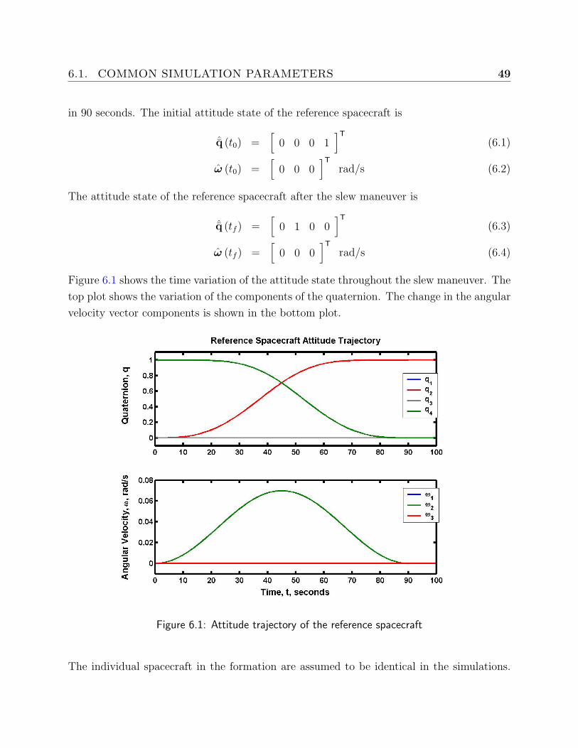
6.1. COMMON SIMULATION PARAMETERS 49

in 90 seconds. The initial attitude state of the reference spacecraft is

ˆq (t0) =[

0 0 0 1]T

(6.1)

ω (t0) =[

0 0 0]T

rad/s (6.2)

The attitude state of the reference spacecraft after the slew maneuver is

ˆq (tf ) =[

0 1 0 0]T

(6.3)

ω (tf ) =[

0 0 0]T

rad/s (6.4)

Figure 6.1 shows the time variation of the attitude state throughout the slew maneuver. The

top plot shows the variation of the components of the quaternion. The change in the angular

velocity vector components is shown in the bottom plot.

Figure 6.1: Attitude trajectory of the reference spacecraft

The individual spacecraft in the formation are assumed to be identical in the simulations.

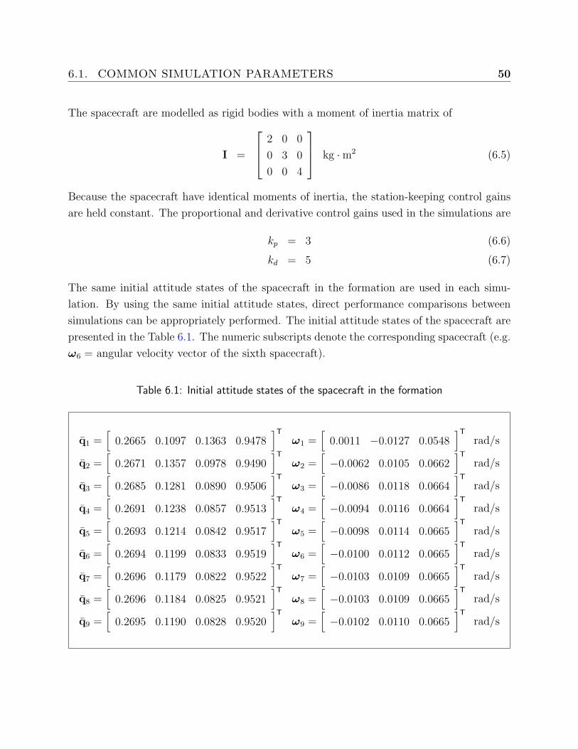
6.1. COMMON SIMULATION PARAMETERS 50

The spacecraft are modelled as rigid bodies with a moment of inertia matrix of

I =

2 0 0

0 3 0

0 0 4

kg ·m2 (6.5)

Because the spacecraft have identical moments of inertia, the station-keeping control gains

are held constant. The proportional and derivative control gains used in the simulations are

kp = 3 (6.6)

kd = 5 (6.7)

The same initial attitude states of the spacecraft in the formation are used in each simu-

lation. By using the same initial attitude states, direct performance comparisons between

simulations can be appropriately performed. The initial attitude states of the spacecraft are

presented in the Table 6.1. The numeric subscripts denote the corresponding spacecraft (e.g.

ω6 = angular velocity vector of the sixth spacecraft).

Table 6.1: Initial attitude states of the spacecraft in the formation

q1 =[

0.2665 0.1097 0.1363 0.9478]T

ω1 =[

0.0011 −0.0127 0.0548]T

rad/s

q2 =[

0.2671 0.1357 0.0978 0.9490]T

ω2 =[−0.0062 0.0105 0.0662

]Trad/s

q3 =[

0.2685 0.1281 0.0890 0.9506]T

ω3 =[−0.0086 0.0118 0.0664

]Trad/s

q4 =[

0.2691 0.1238 0.0857 0.9513]T

ω4 =[−0.0094 0.0116 0.0664

]Trad/s

q5 =[

0.2693 0.1214 0.0842 0.9517]T

ω5 =[−0.0098 0.0114 0.0665

]Trad/s

q6 =[

0.2694 0.1199 0.0833 0.9519]T

ω6 =[−0.0100 0.0112 0.0665

]Trad/s

q7 =[

0.2696 0.1179 0.0822 0.9522]T

ω7 =[−0.0103 0.0109 0.0665

]Trad/s

q8 =[

0.2696 0.1184 0.0825 0.9521]T

ω8 =[−0.0103 0.0109 0.0665

]Trad/s

q9 =[

0.2695 0.1190 0.0828 0.9520]T

ω9 =[−0.0102 0.0110 0.0665

]Trad/s

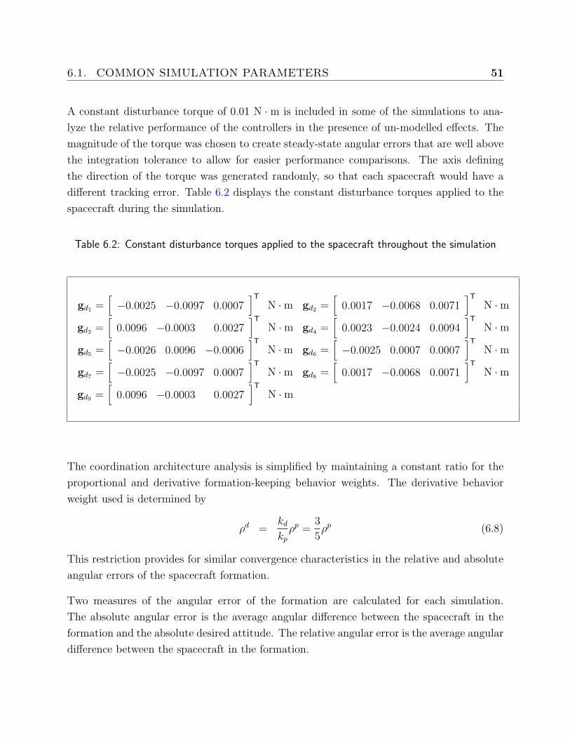
6.1. COMMON SIMULATION PARAMETERS 51

A constant disturbance torque of 0.01 N ·m is included in some of the simulations to ana-

lyze the relative performance of the controllers in the presence of un-modelled effects. The

magnitude of the torque was chosen to create steady-state angular errors that are well above

the integration tolerance to allow for easier performance comparisons. The axis defining

the direction of the torque was generated randomly, so that each spacecraft would have a

different tracking error. Table 6.2 displays the constant disturbance torques applied to the

spacecraft during the simulation.

Table 6.2: Constant disturbance torques applied to the spacecraft throughout the simulation

gd1 =[−0.0025 −0.0097 0.0007

]TN ·m gd2 =

[0.0017 −0.0068 0.0071

]TN ·m

gd3 =[

0.0096 −0.0003 0.0027]T

N ·m gd4 =[

0.0023 −0.0024 0.0094]T

N ·m

gd5 =[−0.0026 0.0096 −0.0006

]TN ·m gd6 =

[−0.0025 0.0007 0.0007

]TN ·m

gd7 =[−0.0025 −0.0097 0.0007

]TN ·m gd8 =

[0.0017 −0.0068 0.0071

]TN ·m

gd9 =[

0.0096 −0.0003 0.0027]T

N ·m

The coordination architecture analysis is simplified by maintaining a constant ratio for the

proportional and derivative formation-keeping behavior weights. The derivative behavior

weight used is determined by

ρd =kd

kp

ρp =3

5ρp (6.8)

This restriction provides for similar convergence characteristics in the relative and absolute

angular errors of the spacecraft formation.

Two measures of the angular error of the formation are calculated for each simulation.

The absolute angular error is the average angular difference between the spacecraft in the

formation and the absolute desired attitude. The relative angular error is the average angular

difference between the spacecraft in the formation.

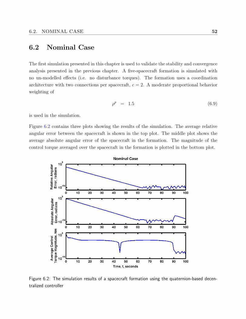
6.2. NOMINAL CASE 52

6.2 Nominal Case

The first simulation presented in this chapter is used to validate the stability and convergence

analysis presented in the previous chapter. A five-spacecraft formation is simulated with

no un-modelled effects (i.e. no disturbance torques). The formation uses a coordination

architecture with two connections per spacecraft, c = 2. A moderate proportional behavior

weighting of

ρp = 1.5 (6.9)

is used in the simulation.

Figure 6.2 contains three plots showing the results of the simulation. The average relative

angular error between the spacecraft is shown in the top plot. The middle plot shows the

average absolute angular error of the spacecraft in the formation. The magnitude of the

control torque averaged over the spacecraft in the formation is plotted in the bottom plot.

Figure 6.2: The simulation results of a spacecraft formation using the quaternion-based decen-

tralized controller

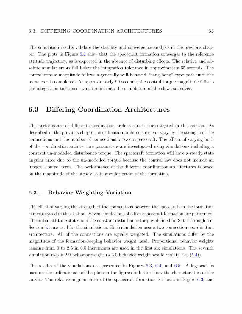
6.3. DIFFERING COORDINATION ARCHITECTURES 53

The simulation results validate the stability and convergence analysis in the previous chap-

ter. The plots in Figure 6.2 show that the spacecraft formation converges to the reference

attitude trajectory, as is expected in the absence of disturbing effects. The relative and ab-

solute angular errors fall below the integration tolerance in approximately 65 seconds. The

control torque magnitude follows a generally well-behaved “bang-bang” type path until the

maneuver is completed. At approximately 90 seconds, the control torque magnitude falls to

the integration tolerance, which represents the completion of the slew maneuver.

6.3 Differing Coordination Architectures

The performance of different coordination architectures is investigated in this section. As

described in the previous chapter, coordination architectures can vary by the strength of the

connections and the number of connections between spacecraft. The effects of varying both

of the coordination architecture parameters are investigated using simulations including a

constant un-modelled disturbance torque. The spacecraft formation will have a steady state

angular error due to the un-modelled torque because the control law does not include an

integral control term. The performance of the different coordination architectures is based

on the magnitude of the steady state angular errors of the formation.

6.3.1 Behavior Weighting Variation

The effect of varying the strength of the connections between the spacecraft in the formation

is investigated in this section. Seven simulations of a five-spacecraft formation are performed.

The initial attitude states and the constant disturbance torques defined for Sat 1 through 5 in

Section 6.1 are used for the simulations. Each simulation uses a two-connection coordination

architecture. All of the connections are equally weighted. The simulations differ by the

magnitude of the formation-keeping behavior weight used. Proportional behavior weights

ranging from 0 to 2.5 in 0.5 increments are used in the first six simulations. The seventh

simulation uses a 2.9 behavior weight (a 3.0 behavior weight would violate Eq. (5.4)).

The results of the simulations are presented in Figures 6.3, 6.4, and 6.5. A log scale is

used on the ordinate axis of the plots in the figures to better show the characteristics of the

curves. The relative angular error of the spacecraft formation is shown in Figure 6.3, and

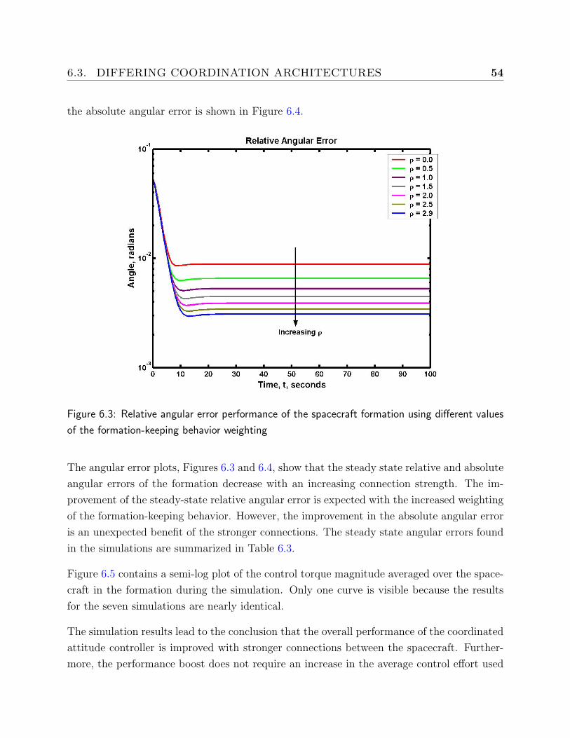
6.3. DIFFERING COORDINATION ARCHITECTURES 54

the absolute angular error is shown in Figure 6.4.

Figure 6.3: Relative angular error performance of the spacecraft formation using different values

of the formation-keeping behavior weighting

The angular error plots, Figures 6.3 and 6.4, show that the steady state relative and absolute

angular errors of the formation decrease with an increasing connection strength. The im-

provement of the steady-state relative angular error is expected with the increased weighting

of the formation-keeping behavior. However, the improvement in the absolute angular error

is an unexpected benefit of the stronger connections. The steady state angular errors found

in the simulations are summarized in Table 6.3.

Figure 6.5 contains a semi-log plot of the control torque magnitude averaged over the space-

craft in the formation during the simulation. Only one curve is visible because the results

for the seven simulations are nearly identical.

The simulation results lead to the conclusion that the overall performance of the coordinated

attitude controller is improved with stronger connections between the spacecraft. Further-

more, the performance boost does not require an increase in the average control effort used

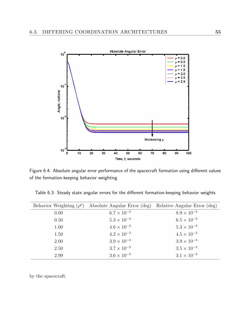
6.3. DIFFERING COORDINATION ARCHITECTURES 55

Figure 6.4: Absolute angular error performance of the spacecraft formation using different values

of the formation-keeping behavior weighting

Table 6.3: Steady state angular errors for the different formation-keeping behavior weights

Behavior Weighting (ρp) Absolute Angular Error (deg) Relative Angular Error (deg)

0.00 6.7× 10−3 8.9× 10−3

0.50 5.3× 10−3 6.5× 10−3

1.00 4.6× 10−3 5.3× 10−3

1.50 4.2× 10−3 4.5× 10−3

2.00 3.9× 10−3 3.9× 10−3

2.50 3.7× 10−3 3.5× 10−3

2.99 3.6× 10−3 3.1× 10−3

by the spacecraft.

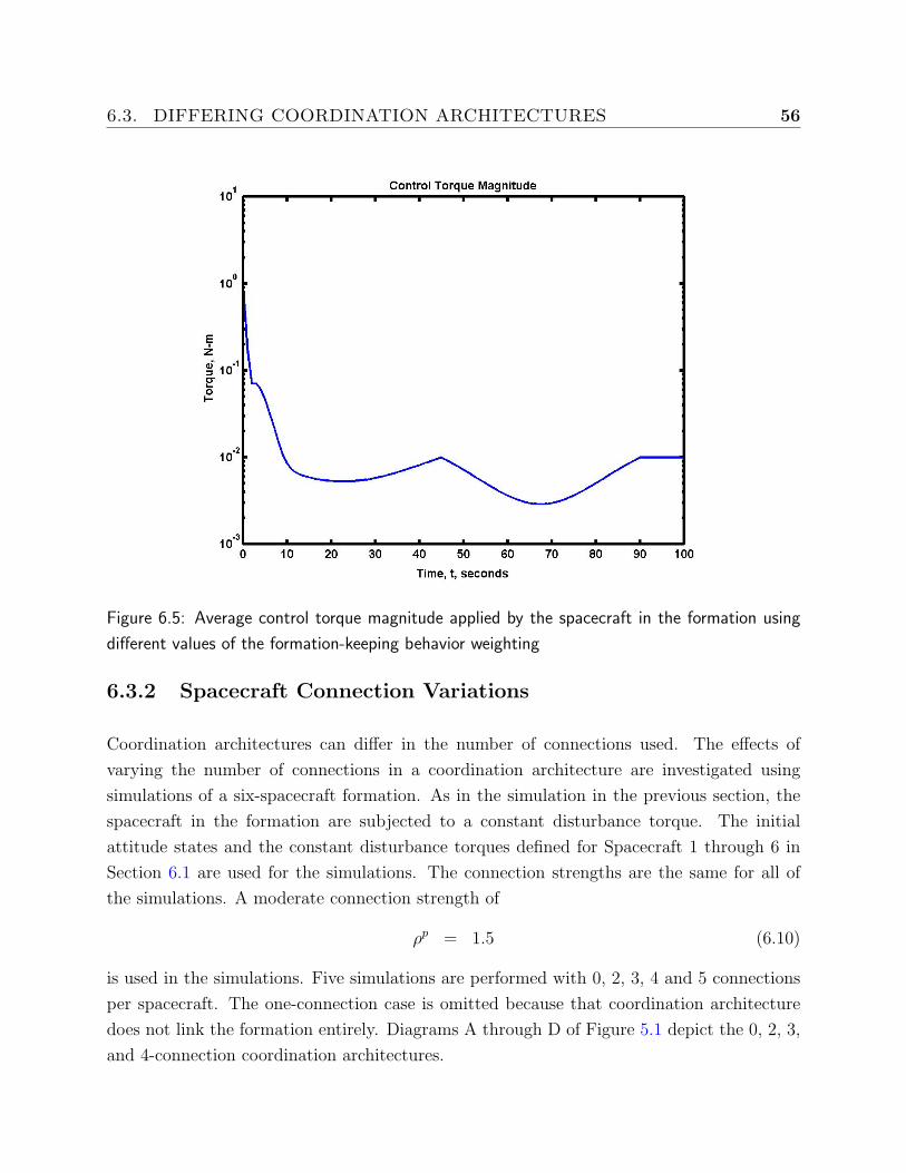
6.3. DIFFERING COORDINATION ARCHITECTURES 56

Figure 6.5: Average control torque magnitude applied by the spacecraft in the formation using

different values of the formation-keeping behavior weighting

6.3.2 Spacecraft Connection Variations

Coordination architectures can differ in the number of connections used. The effects of

varying the number of connections in a coordination architecture are investigated using

simulations of a six-spacecraft formation. As in the simulation in the previous section, the

spacecraft in the formation are subjected to a constant disturbance torque. The initial

attitude states and the constant disturbance torques defined for Spacecraft 1 through 6 in

Section 6.1 are used for the simulations. The connection strengths are the same for all of

the simulations. A moderate connection strength of

ρp = 1.5 (6.10)

is used in the simulations. Five simulations are performed with 0, 2, 3, 4 and 5 connections

per spacecraft. The one-connection case is omitted because that coordination architecture

does not link the formation entirely. Diagrams A through D of Figure 5.1 depict the 0, 2, 3,

and 4-connection coordination architectures.

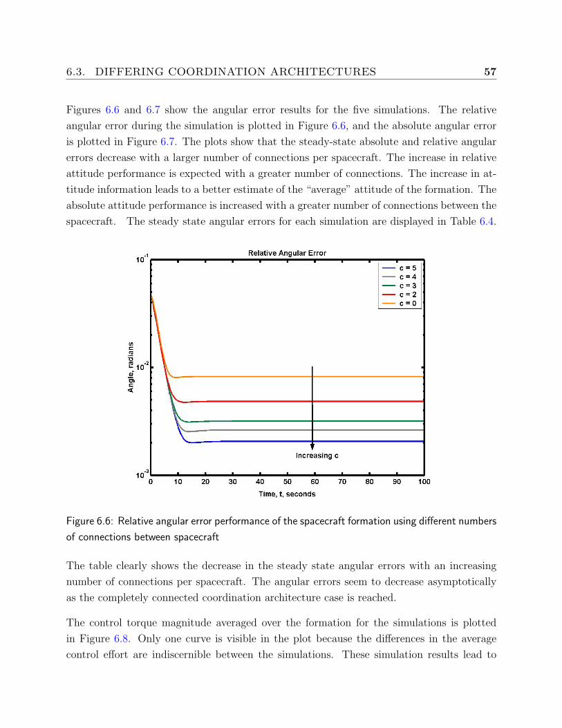
6.3. DIFFERING COORDINATION ARCHITECTURES 57

Figures 6.6 and 6.7 show the angular error results for the five simulations. The relative

angular error during the simulation is plotted in Figure 6.6, and the absolute angular error

is plotted in Figure 6.7. The plots show that the steady-state absolute and relative angular

errors decrease with a larger number of connections per spacecraft. The increase in relative

attitude performance is expected with a greater number of connections. The increase in at-

titude information leads to a better estimate of the “average” attitude of the formation. The

absolute attitude performance is increased with a greater number of connections between the

spacecraft. The steady state angular errors for each simulation are displayed in Table 6.4.

Figure 6.6: Relative angular error performance of the spacecraft formation using different numbers

of connections between spacecraft

The table clearly shows the decrease in the steady state angular errors with an increasing

number of connections per spacecraft. The angular errors seem to decrease asymptotically

as the completely connected coordination architecture case is reached.

The control torque magnitude averaged over the formation for the simulations is plotted

in Figure 6.8. Only one curve is visible in the plot because the differences in the average

control effort are indiscernible between the simulations. These simulation results lead to

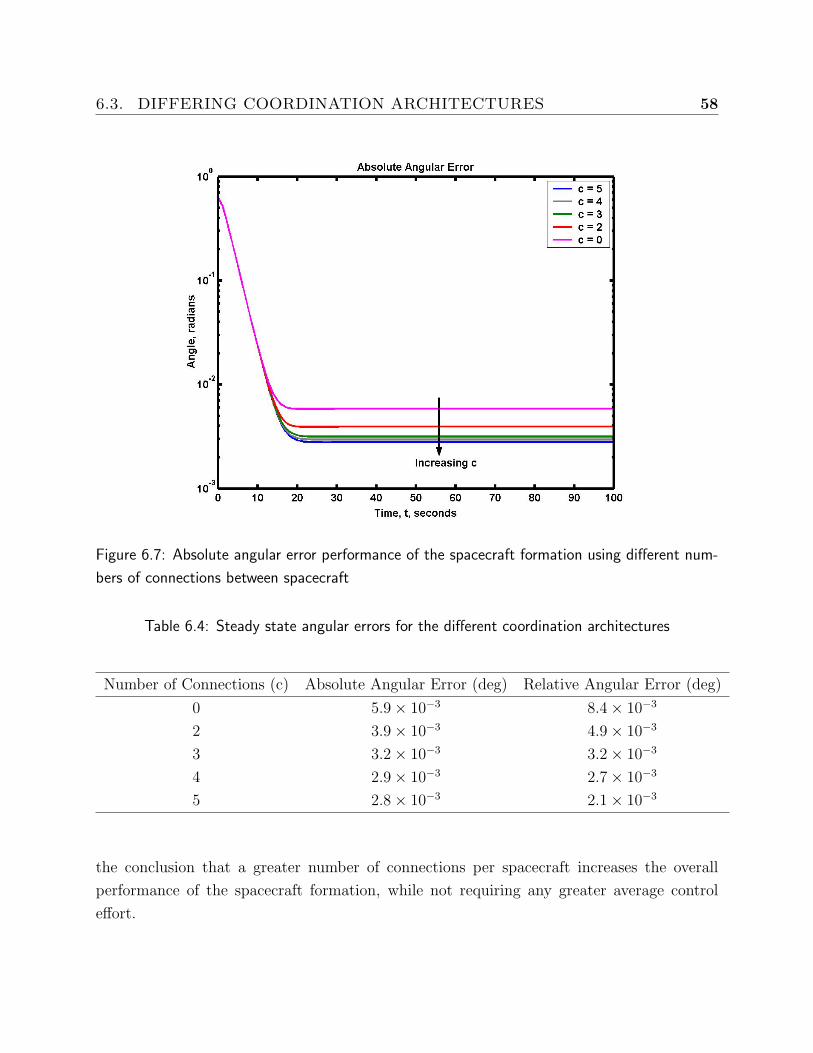
6.3. DIFFERING COORDINATION ARCHITECTURES 58

Figure 6.7: Absolute angular error performance of the spacecraft formation using different num-

bers of connections between spacecraft

Table 6.4: Steady state angular errors for the different coordination architectures

Number of Connections (c) Absolute Angular Error (deg) Relative Angular Error (deg)

0 5.9× 10−3 8.4× 10−3

2 3.9× 10−3 4.9× 10−3

3 3.2× 10−3 3.2× 10−3

4 2.9× 10−3 2.7× 10−3

5 2.8× 10−3 2.1× 10−3

the conclusion that a greater number of connections per spacecraft increases the overall

performance of the spacecraft formation, while not requiring any greater average control

effort.

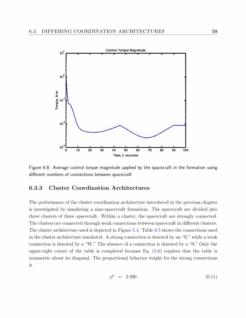
6.3. DIFFERING COORDINATION ARCHITECTURES 59

Figure 6.8: Average control torque magnitude applied by the spacecraft in the formation using

different numbers of connections between spacecraft

6.3.3 Cluster Coordination Architectures

The performance of the cluster coordination architecture introduced in the previous chapter

is investigated by simulating a nine-spacecraft formation. The spacecraft are divided into

three clusters of three spacecraft. Within a cluster, the spacecraft are strongly connected.

The clusters are connected through weak connections between spacecraft in different clusters.

The cluster architecture used is depicted in Figure 5.4. Table 6.5 shows the connections used

in the cluster architecture simulated. A strong connection is denoted by an “S,” while a weak

connection is denoted by a “W.” The absence of a connection is denoted by a “0.” Only the

upper-right corner of the table is completed because Eq. (5.6) requires that the table is

symmetric about its diagonal. The proportional behavior weight for the strong connections

is

ρp = 2.990 (6.11)

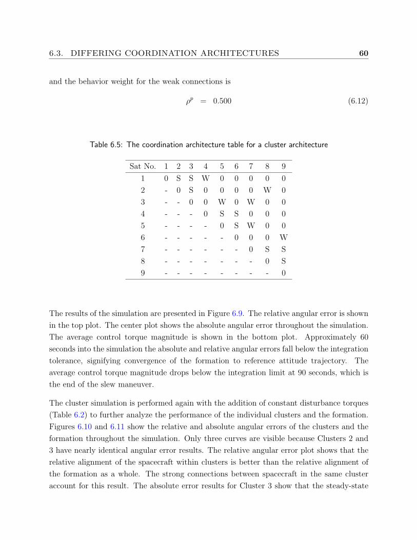
6.3. DIFFERING COORDINATION ARCHITECTURES 60

and the behavior weight for the weak connections is

ρp = 0.500 (6.12)

Table 6.5: The coordination architecture table for a cluster architecture

Sat No. 1 2 3 4 5 6 7 8 9

1 0 S S W 0 0 0 0 0

2 - 0 S 0 0 0 0 W 0

3 - - 0 0 W 0 W 0 0

4 - - - 0 S S 0 0 0

5 - - - - 0 S W 0 0

6 - - - - - 0 0 0 W

7 - - - - - - 0 S S

8 - - - - - - - 0 S

9 - - - - - - - - 0

The results of the simulation are presented in Figure 6.9. The relative angular error is shown

in the top plot. The center plot shows the absolute angular error throughout the simulation.

The average control torque magnitude is shown in the bottom plot. Approximately 60

seconds into the simulation the absolute and relative angular errors fall below the integration

tolerance, signifying convergence of the formation to reference attitude trajectory. The

average control torque magnitude drops below the integration limit at 90 seconds, which is

the end of the slew maneuver.

The cluster simulation is performed again with the addition of constant disturbance torques

(Table 6.2) to further analyze the performance of the individual clusters and the formation.

Figures 6.10 and 6.11 show the relative and absolute angular errors of the clusters and the

formation throughout the simulation. Only three curves are visible because Clusters 2 and

3 have nearly identical angular error results. The relative angular error plot shows that the

relative alignment of the spacecraft within clusters is better than the relative alignment of

the formation as a whole. The strong connections between spacecraft in the same cluster

account for this result. The absolute error results for Cluster 3 show that the steady-state

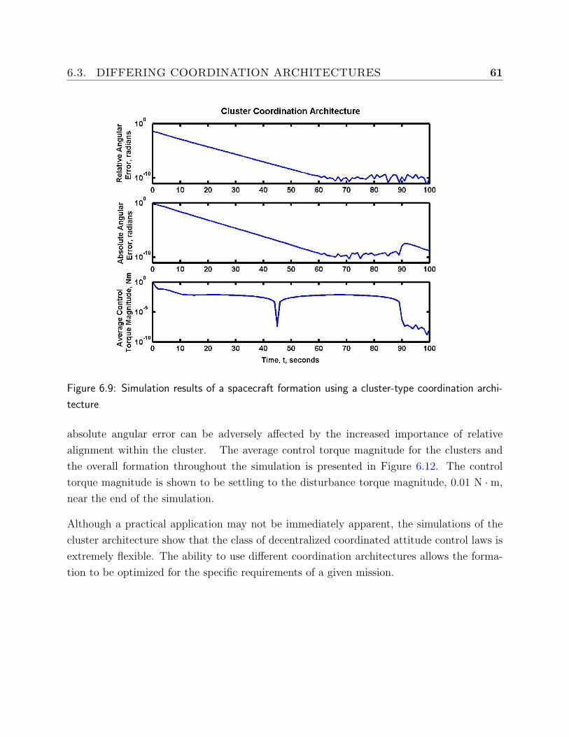
6.3. DIFFERING COORDINATION ARCHITECTURES 61

Figure 6.9: Simulation results of a spacecraft formation using a cluster-type coordination archi-

tecture

absolute angular error can be adversely affected by the increased importance of relative

alignment within the cluster. The average control torque magnitude for the clusters and

the overall formation throughout the simulation is presented in Figure 6.12. The control

torque magnitude is shown to be settling to the disturbance torque magnitude, 0.01 N ·m,

near the end of the simulation.

Although a practical application may not be immediately apparent, the simulations of the

cluster architecture show that the class of decentralized coordinated attitude control laws is

extremely flexible. The ability to use different coordination architectures allows the forma-

tion to be optimized for the specific requirements of a given mission.

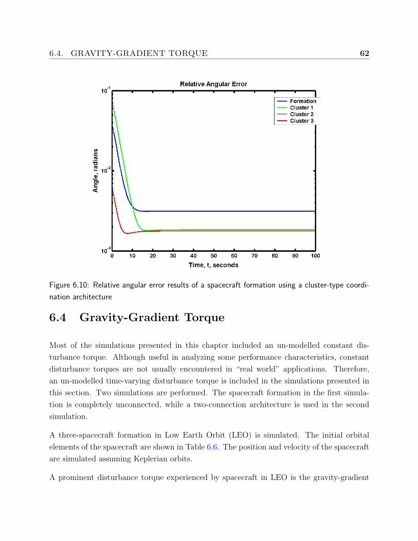
6.4. GRAVITY-GRADIENT TORQUE 62

Figure 6.10: Relative angular error results of a spacecraft formation using a cluster-type coordi-

nation architecture

6.4 Gravity-Gradient Torque

Most of the simulations presented in this chapter included an un-modelled constant dis-

turbance torque. Although useful in analyzing some performance characteristics, constant

disturbance torques are not usually encountered in “real world” applications. Therefore,

an un-modelled time-varying disturbance torque is included in the simulations presented in

this section. Two simulations are performed. The spacecraft formation in the first simula-

tion is completely unconnected, while a two-connection architecture is used in the second

simulation.

A three-spacecraft formation in Low Earth Orbit (LEO) is simulated. The initial orbital

elements of the spacecraft are shown in Table 6.6. The position and velocity of the spacecraft

are simulated assuming Keplerian orbits.

A prominent disturbance torque experienced by spacecraft in LEO is the gravity-gradient

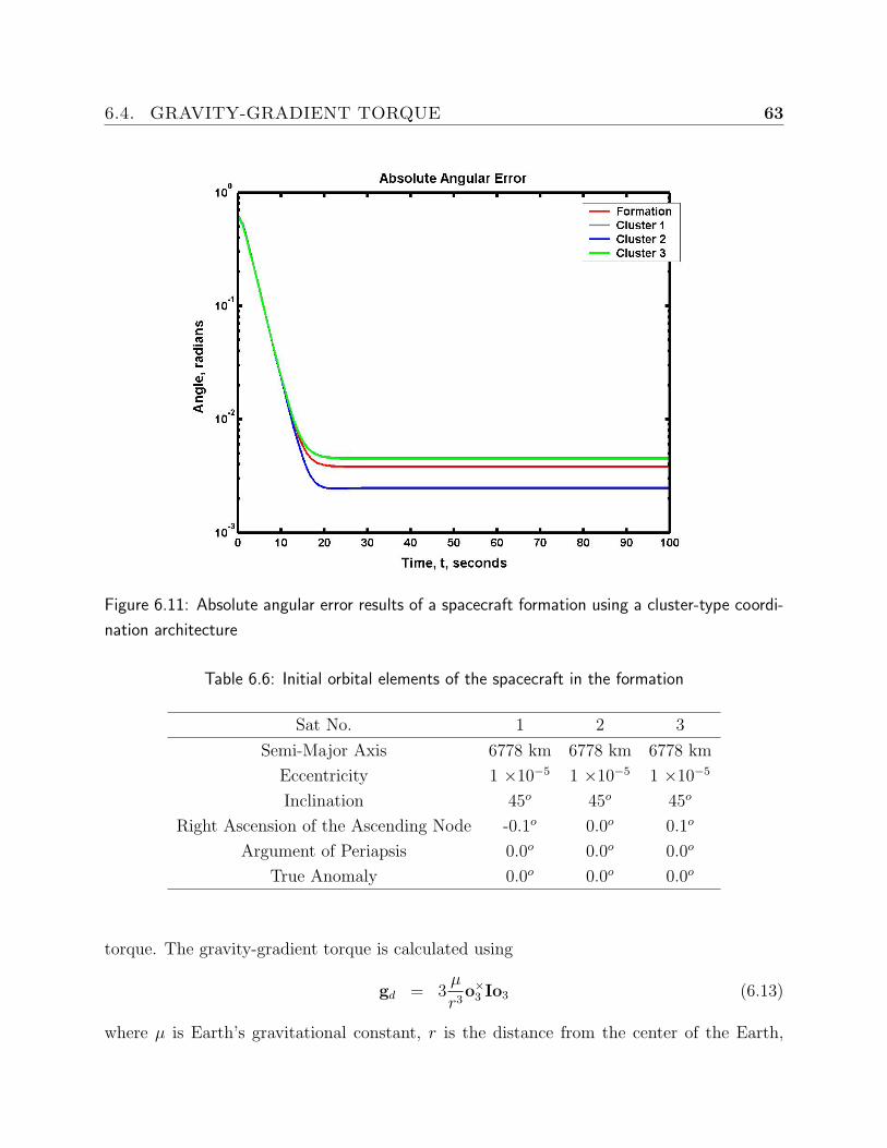
6.4. GRAVITY-GRADIENT TORQUE 63

Figure 6.11: Absolute angular error results of a spacecraft formation using a cluster-type coordi-

nation architecture

Table 6.6: Initial orbital elements of the spacecraft in the formation

Sat No. 1 2 3

Semi-Major Axis 6778 km 6778 km 6778 km

Eccentricity 1 ×10−5 1 ×10−5 1 ×10−5

Inclination 45o 45o 45o

Right Ascension of the Ascending Node -0.1o 0.0o 0.1o

Argument of Periapsis 0.0o 0.0o 0.0o

True Anomaly 0.0o 0.0o 0.0o

torque. The gravity-gradient torque is calculated using

gd = 3µ

r3o×3 Io3 (6.13)

where µ is Earth’s gravitational constant, r is the distance from the center of the Earth,

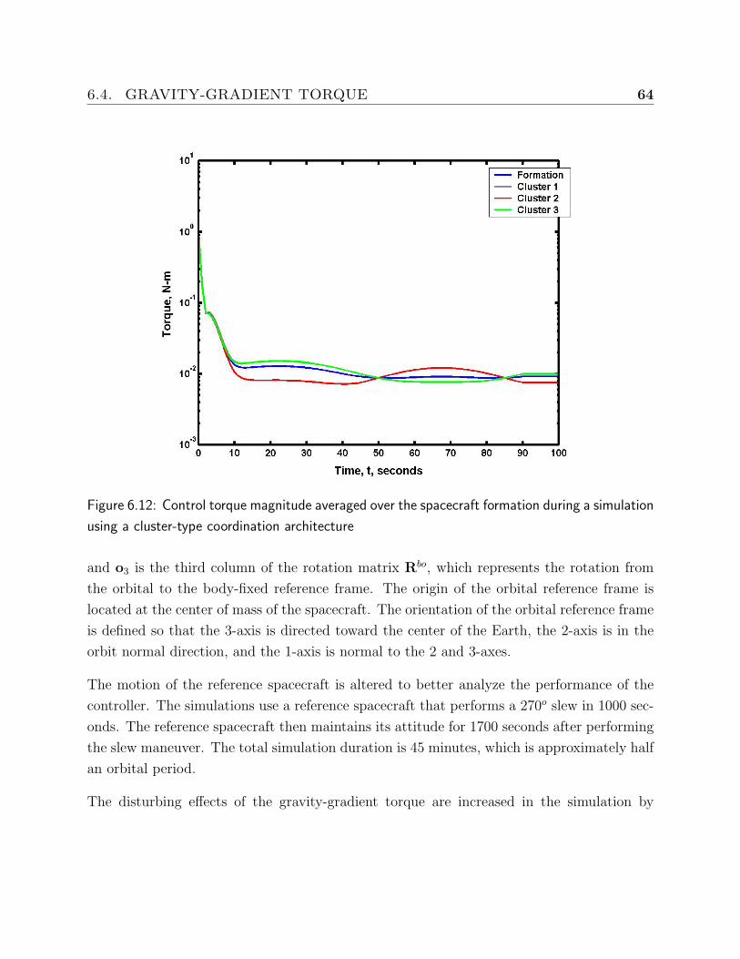
6.4. GRAVITY-GRADIENT TORQUE 64

Figure 6.12: Control torque magnitude averaged over the spacecraft formation during a simulation

using a cluster-type coordination architecture

and o3 is the third column of the rotation matrix Rbo, which represents the rotation from

the orbital to the body-fixed reference frame. The origin of the orbital reference frame is

located at the center of mass of the spacecraft. The orientation of the orbital reference frame

is defined so that the 3-axis is directed toward the center of the Earth, the 2-axis is in the

orbit normal direction, and the 1-axis is normal to the 2 and 3-axes.

The motion of the reference spacecraft is altered to better analyze the performance of the

controller. The simulations use a reference spacecraft that performs a 270o slew in 1000 sec-

onds. The reference spacecraft then maintains its attitude for 1700 seconds after performing

the slew maneuver. The total simulation duration is 45 minutes, which is approximately half

an orbital period.

The disturbing effects of the gravity-gradient torque are increased in the simulation by

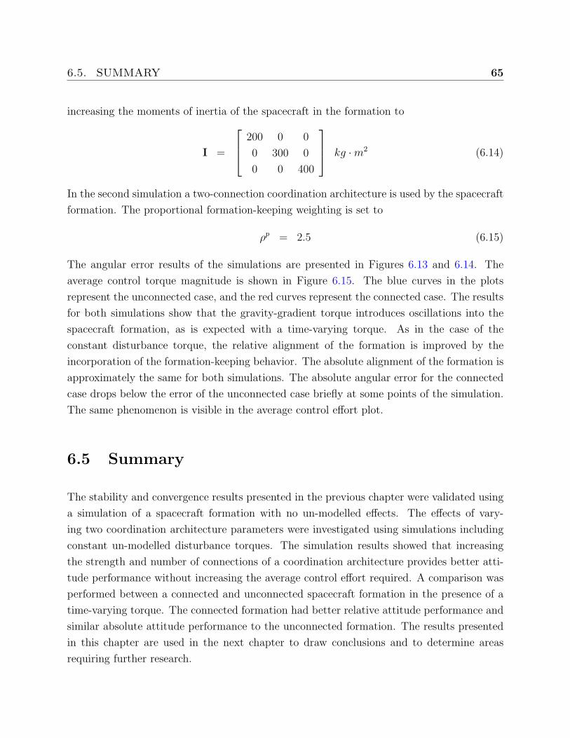
6.5. SUMMARY 65

increasing the moments of inertia of the spacecraft in the formation to

I =

200 0 0

0 300 0

0 0 400

kg ·m2 (6.14)

In the second simulation a two-connection coordination architecture is used by the spacecraft

formation. The proportional formation-keeping weighting is set to

ρp = 2.5 (6.15)

The angular error results of the simulations are presented in Figures 6.13 and 6.14. The

average control torque magnitude is shown in Figure 6.15. The blue curves in the plots

represent the unconnected case, and the red curves represent the connected case. The results

for both simulations show that the gravity-gradient torque introduces oscillations into the

spacecraft formation, as is expected with a time-varying torque. As in the case of the

constant disturbance torque, the relative alignment of the formation is improved by the

incorporation of the formation-keeping behavior. The absolute alignment of the formation is

approximately the same for both simulations. The absolute angular error for the connected

case drops below the error of the unconnected case briefly at some points of the simulation.

The same phenomenon is visible in the average control effort plot.

6.5 Summary

The stability and convergence results presented in the previous chapter were validated using

a simulation of a spacecraft formation with no un-modelled effects. The effects of vary-

ing two coordination architecture parameters were investigated using simulations including

constant un-modelled disturbance torques. The simulation results showed that increasing

the strength and number of connections of a coordination architecture provides better atti-

tude performance without increasing the average control effort required. A comparison was

performed between a connected and unconnected spacecraft formation in the presence of a

time-varying torque. The connected formation had better relative attitude performance and

similar absolute attitude performance to the unconnected formation. The results presented

in this chapter are used in the next chapter to draw conclusions and to determine areas

requiring further research.

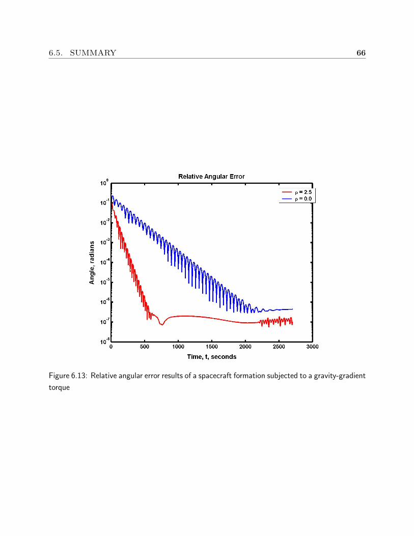
6.5. SUMMARY 66

Figure 6.13: Relative angular error results of a spacecraft formation subjected to a gravity-gradient

torque

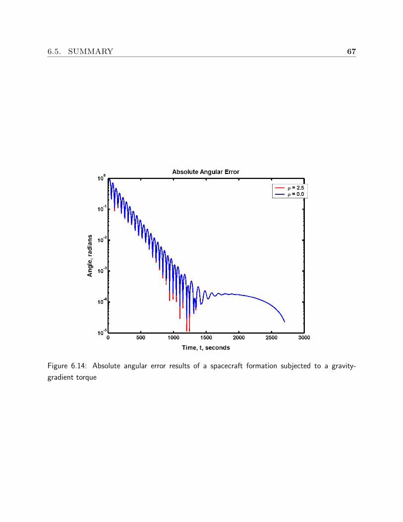
6.5. SUMMARY 67

Figure 6.14: Absolute angular error results of a spacecraft formation subjected to a gravity-

gradient torque

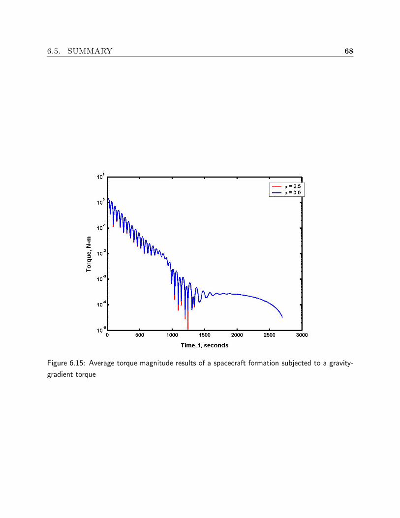
6.5. SUMMARY 68

Figure 6.15: Average torque magnitude results of a spacecraft formation subjected to a gravity-

gradient torque

69

Chapter 7

Summary & Conclusions

Spacecraft formations offer more powerful and robust space system architectures than single

spacecraft systems. Investigations into the dynamics and control of spacecraft formations are

vital for the development and design of future successful space missions. The primary con-

tribution of this work is the development and analysis of a class of decentralized coordinated

attitude tracking control laws that guarantee global convergence of a spacecraft formation’s

attitude.

Special emphasis is placed on developing physically significant relative attitude variables,

and providing a global convergence proof for the class of decentralized attitude control laws.

These areas are inadequately addressed in prior literature on the topic. The relative attitude

quaternion and relative angular velocity vector are developed as physically significant relative

attitude variables. These variables are used in the development of the attitude control laws.

Lyapunov stability theory is used to prove that the class of decentralized attitude control

laws guarantee the global convergence of the spacecraft formation’s attitude. The results of

a numeric simulation of a five-spacecraft formation performing a slew maneuver reinforced

the convergence results.

The class of decentralized attitude control laws consists of control laws that use different

coordination architectures. Coordination architectures can vary by the number and strength

of the connections between spacecraft. The performance effects of varying these two co-

ordination architecture variables are investigated using numeric simulations of a spacecraft

formation with constant applied disturbance torques.

70

The simulation results show that increasing either the number or strength of the connec-

tions decreases the steady-state relative and absolute angular errors caused by the constant

disturbance torques without increasing the average control effort required. The decrease in

the steady-state relative angular error is expected because with an increase in the number

or strength of the connections between spacecraft a greater importance is placed on the

relative alignment by the decentralized attitude control laws. However, the decrease in the

steady-state absolute angular error is unexpected. The gravity-gradient torque simulation

results further complicate this matter. In that simulation, an increase in the number and

strength of the connections leads to better relative alignment, but does not provide any

absolute alignment benefit.

The physical reasoning behind the results for the absolute alignment in the different simula-

tions is not readily apparent, and warrants further investigation. Analytic analysis into the

effects of un-modelled disturbance torques on the formation may be useful in determining

the cause of this phenomenon. Another area for further analysis is the effect of imperfect

communication on the performance of the control laws. Particularly interesting would be the

use of a sequential filter to alleviate some of the dependency of the control laws on continuous

communication between the spacecraft.

During the course of this research the author noted several possible extensions to this work.

The first logical extension would be the addition of an integral control term to counteract

constant or slow-varying disturbance torques. However, the author is quick to note that the

use of an integral control term in the presence of conflicting control aims could lead to situa-

tions where the formation-keeping control action is simply cancelled out by a station-keeping

integral control term. Possibly the most interesting extension would be the application of

the coordinated control approach used in this work to the orbital control of a spacecraft for-

mation. It is believed by the author that the similar form of the relative position variables

and the relative attitude variables would also allow several of the analytic techniques used

in this work to be applied to the problem.

71

References

[1] P. Wang and F. Hadaegh, “Coordination and control of multiple microspacecraft moving

in formation,” The Journal of the Astronautical Sciences, vol. 44, pp. 315–355, July-

September 1996.

[2] P. Wang, F. Hadaegh, and K. Lau, “Synchronized Formation Rotation and Attitude

Control of Multiple Free-Flying Spacecraft,” Journal of Guidance, Control, and Dy-

namics, vol. 22, pp. 28–35, January-February 1999.

[3] P. Wang, J. Yeh, and F. Hadaegh, “Synchronized Rotation of Multiple Autonomous

Spacecraft with Rule-Based Controls: Experimental Study,” Journal of Guidance, Con-

trol, and Dynamics, vol. 24, pp. 352–359, March-April 2001.

[4] W. Kang, A. Sparks, and S. Banda, “Coordinated Control of Multisatellite Systems,”

Journal of Guidance, Control, and Dynamics, vol. 24, pp. 360–368, March-April 2001.

[5] W. Kang and H.-H. Yeh, “Co-ordinated attitude control of multi-satellite systems,”

International Journal of Robust and Nonlinear Control, vol. 12, pp. 185–205, February-

March 2002.

[6] W. Kang, N. Xi, and A. Sparks, “Theory and applications of formation control in a

perceptive referenced frame,” in Proceedings of the IEEE Conference on Decision and

Control, (Sidney), December 2000.

[7] W. Kang, H.-H. Yeh, and A. Sparks, “Coordinated Control of Relative Attitude for

Satellite Formation,” in Guidance, Naviagtion, and Control Conference and Exhibit,

(Montreal, Canada), AIAA 2001-4093, August 2001.

[8] W. Kang and A. Sparks, “Coordinated Attitude and Formation Control of Multi-

satellite Systems,” in Guidance, Naviagtion, and Control Conference and Exhibit, (Mon-

terey, California), AIAA 2002-4655, August 2002.

REFERENCES 72

[9] W. Ren and R. W. Beard, “Virtual Structure Based Spacecraft Formation Control with

Formation Feedback,” in AIAA Guidance, Navigation, and Control Conference and

Exhibit, (Monterey, California), AIAA 2002-4963, August 2002.

[10] J. Lawton, R. W. Beard, and F. Y. Hadaegh, “Elementary Attitude Formation Maneu-

vers Via Leader-following and Behavior-based Control,” in Guidance, Naviagtion, and

Control Conference and Exhibit, (Denver, Colorado), AIAA 2000-4442, August 2000.

[11] R. W. Beard, J. Lawton, and F. Y. Hadaegh, “A feedback architecture for formation

control,” in American Control Conference, (Chicago, IL), June 2000.

[12] J. Lawton, B. Young, and R. Beard, “A decentralized approach to elementarty formatoin

maneuvers,” in Proceedings of The IEEE International Conference on Robotics and

Automation, (San Fransico, CA), April 2000.

[13] R. Beard, J. Lawton, and F. Hadaegh, “A feedback architecture for formation control,”

IEEE Transactions on Control Systems Technology, vol. 9, no. 6, pp. 777–790, 2001.

[14] J. R. Lawton and R. W. Beard, “Synchronized multiple spacecraft rotations,” Automat-

ica, vol. 38, pp. 1359–1364, August 2002.

[15] A. Das, R. Cobb, and M. Stallard, “TechSat 21 - A Revolutionary Concept in Dis-

tributed Space Based Sensing,” in Proceedings of the guidance, navigatin and control

conference, vol. AIAA-98-5255, (Boston, MA), pp. 1–6, AIAA, August 1998.

[16] J. Leitner, F. Bauer, D. Folta, M. Moreau, R. Carpenter, and J. How, “Formation Flight

in Space,” GPS World, February 2002.

[17] A. DeCou, “Orbital station-keeping for multiple spacecraft interferometry,” Journal of

the Astronautical Sciences, vol. 39, pp. 283–297, July-September 1991.

[18] E. Davison, “The Decentralized Stabilization and Control of a Class of Unknown Non-

Linear Time-Varying Systems,” Automatica, vol. 10, pp. 309–316, 1974.

[19] M. Aoki and M. T. Li, “Partial Reconstruction of State Vector in Decentralized Dynamic

Systems,” IEEE Transactions on Automatic Control, vol. 18, pp. 289–292, June 1973.

[20] T. Balch and R. C. Arkin, “Behavior-Based Formation Control for Multirobot Teams,”

IEEE Transactions on Robotics and Automation, vol. 14, pp. 926–939, December 1998.

[21] C. Lindensmith (Ed.), “Technology Plan for the Terrestrial Planet Finder,” JPL Pub-

lication 03-007, NASA Jet Propulsion Laboratory, California Institute of Technology,

Pasadena, California, March 2003.

REFERENCES 73

[22] K. Alfriend, “Dynamics and Control of Formation Flying Satellites.” Virginia Tech

Aerospace and Ocean Engineering Department Graduate Seminar, September 18 2003.

[23] P. C. Hughes, Spacecraft Attitude Dynamics. New York: John Wiley and Sons, 1986.

[24] C. D. Hall, “Class Notes - Spacecraft Attitude Dynamics and Control.” January 12,

2003.

[25] H. Schaub and J. L. Junkins, Analytical Mechanics of Space Systems. AIAA Education

Series, Reston, Virginia: American Institute of Aeronautics and Astronautics, 2003.

[26] H. K. Khalil, Nonlinear Systems. New York, New York: MacMillan, 1992.

[27] R. Mortensen, “A Globally Stable Linear Attitude Regulator,” International Journal of

Control, vol. 8, pp. 297–302, 1968.

[28] P. Tsiotras, “New Control Laws for the Attitude Stabilization of Rigid Bodies,” in 13th

IFAC Symposium on Automatic Control in Aerospace, pp. 316–321, September 1994.

[29] R. L. Burden and J. D. Faires, Numerical Analysis 7th Edition. Pacific Grove, California:

Brooks/Cole, 2001.

74

Vita

Matthew Clark VanDyke was born in Havre de Grace, Maryland. He attended Rising Sun

High School, where he graduated in June 1998 with honors. Matt started at Virginia Tech

in the Fall of 1998. He received his bachelor’s degree in Aerospace Engineering in Spring

1999.