attosecond optical and electronic wave packets...dig. kemiska reaktioner d¨ar atomer och molekyler...
TRANSCRIPT

Attosecond Optical andElectronic Wave Packets
Per Johnsson
Doctoral Thesis
2006

Attosecond Optical and Electronic Wave Packets
Copyright c© 2006 Per JohnssonAll rights reservedPrinted in Sweden by KFS AB, Lund, 2006
Division of Atomic PhysicsDepartment of PhysicsFaculty of Engineering LTHLund UniversityP.O. Box 118SE–221 00 LundSweden
ISSN 0281-2762Lund Reports on Atomic Physics, LRAP-363
ISBN 13: 978-91-628-6898-7ISBN 10: 91-628-6898-5

Abstract
When a low-frequency laser pulse is focused to a high intensity ina gas, the electric field of the laser may become comparable to, oreven exceed, the electric field between the electrons and the nucleusin the atom. Under such conditions, through a process knownas high-order harmonic generation, bursts of extreme ultravioletradiation may be emitted, with durations in the attosecond domain(1 as = 10−18 s), which is the time-scale of electronic processes. Inthe work presented in this thesis, attosecond pulse trains (APTs)have been generated in the laboratory. These APTs have furtherbeen characterized and finally used in a number of applications.
The first series of experiments was focused on the generation,control and characterization of high-order harmonics on the fem-tosecond time-scale, corresponding to the duration of the drivingpulse. The time-frequency structure of individual harmonics doesnot significantly affect the properties of the individual attosecondpulses, but is, however, important for the overall structure of theAPT, which is also the subject of some theoretical investigationsincluded in this work.
In the second series of experiments, the production and mea-surement of attosecond pulses in an APT were successfully per-formed. In addition, external phase control of the attosecondpulses was demonstrated, by means of metallic filters, leading topost-compression of the pulses down to a duration of 170 as, whichwas, at that time, the shortest pulse duration ever reported.
Finally, the APTs were applied to inject electron wave pack-ets (EWPs), through single-photon ionization, into an externallow-frequency laser field. By using the pulses in the APT to ob-tain precise timing of the ionization, control of the ejected EWPs,and even of the ionization process itself, by the external field, wasdemonstrated. It has also been shown that, making use of theexternal control offered by the APTs, it is possible to perform in-terference experiments on continuum EWPs, in a way very similarto that of traditional interference experiments with photons.
iii


Sammanfattning
Vill man ta en bild av nagot som ror sig mycket snabbt, kravs detatt man anvander en kort exponeringstid. Om kamerans slutare aroppen under for lang tid, hinner det man vill fotografera rora sigunder tiden filmen exponeras, med resultatet att bilden blir sud-dig. Kemiska reaktioner dar atomer och molekyler ar inblandadear exempel pa nagot som sker pa valdigt kort tid, typiskt nagrahundra femtosekunder (en femtosekund ar en miljondels miljard-dels sekund). For att kunna tidsupplosa dessa har forskare underde senaste tjugo aren anvant ultrakorta laserpulser, bade till attstarta reaktionen, och for att mata resultatet.
Omfordelningen av elektroner som befinner sig i nagot av deinre elektronskalen, nara atomkarnan, ar exempel pa en processsom ar annu snabbare. Denna sker typiskt pa en attosekunds-tidsskala, dar en attosekund (as) ar en miljarddels miljarddelssekund, dvs. tusen ganger kortare an en femtosekund. Sa kortaljuspulser kan bara skapas genom att anvanda vaglangder i det ex-tremt ultravioletta omradet, vilket innebar vaglangder kortare an100 nm. Detta lyckades en grupp forskare med for forsta gangen ar2001, genom generering av hoga overtoner till en intensiv infrarodlaserpuls.
Det arbete som ligger till grund for denna avhandling, syft-ade i forsta hand till att generera, karakterisera och kontrolleraattosekundspulser, och i andra hand till att aven anvanda dessa itillampningar. Denna avhandling beskriver ett antal experimentmed detta som mal, gjorda vid Hogeffektlaserfaciliteten vid LundsTekniska Hogskola.
I ett experiment, utfort ar 2003, genererades och karakter-iserades for forsta gangen attosekundspulser i Lund, utsanda i ettpulstag dar varje puls hade en varaktighet pa 250 as. Som enfortsattning pa detta experiment anvandes tunna filter gjorda avaluminium for att kontrollera fasen pa attosekundspulserna, ochpa sa vis kunde dessa komprimeras till en pulslangd pa endast170 as, som vid denna tid utgjorde det nya varldsrekordet.
Parallellt med experimenten med attosekundspulser, har ocksatidsstrukturen hos de enskilda overtoner som bygger upp pulstagetstuderats, bade experimentellt och teoretiskt. De enskilda overton-
v

Sammanfattning
ernas struktur har ingen storre paverkan pa varje enskild puls,utan paverkar istallet variationen mellan pulserna i taget. I dessastudier pavisades bland annat hur man genom att kontrollera tids-strukturen hos den laserpuls som genererar overtonerna, kan kon-trollera tidsstrukturen hos attosekundspulstaget.
I nagra av de senast gjorda experimenten anvandes attosek-undspulserna till att skapa fria elektroner, genom jonisation aven gas, och genom att overlappa attosekundspulstaget med ettinfrarott laserfalt, kunde de skapade elektronerna styras och de-ras slutliga hastighet kontrolleras. Elektronernas egenskaper dade skapas beror pa tidsstrukturen hos attosekundspulserna, och iett av experimenten visas hur man genom att kontrollera denna,kan paverka vad som hander med elektronerna i laserfaltet. Vidarevisades i ett experiment hur man genom att anvanda attosekund-spulser, som inte i sig sjalva har tillrackligt hog energi for att joni-sera atomerna i gasen, kan kontrollera sjalva jonisationsprocessenmed hjalp av det infraroda laserfaltet.
Enligt kvantmekaniken ar alla partiklar aven vagor, och viceversa, vilket innebar att de elektroner som skapas och kontrollerasi de experiment som namnts ovan, aven borde kunna betraktas somvagpaket. I ett av de presenterade experimenten framgar detta iallra hogsta grad, da ett infrarott laserfalt anvandes for att fa tvaolika delar av ett sadant elektronvagpaket, som fran borjan hadeolika riktning och hastighet, till att slutligen fa samma riktningoch hastighet. I experimentet observerades da interferens mellandessa olika bidrag, ett fenomen som oftast associeras med optiskaexperiment, och fran denna interferens kunde information om fasenhos elektronvagpaketen fas.
vi

List of Publications
This thesis is based on the following papers, which will be referredto by their roman numerals in the text.
I Characterization of High-Order HarmonicRadiation on Femtosecond and Attosecond TimeScalesR. Lopez-Martens, J. Mauritsson, P. Johnsson, K. Varju,A. L’Huillier, W. Kornelis, J. Biegert, U. Keller, M. Gaardeand K. Schafer.Appl. Phys B 78, 835 (2004).
II Amplitude and Phase Control of Attosecond LightPulsesR. Lopez-Martens, K. Varju, P. Johnsson, J. Mauritsson,Y. Mairesse, P. Salieres, M. B. Gaarde, K. J. Schafer,A. Persson, S. Svanberg, C.-G. Wahlstrom andA. L’Huillier.Phys. Rev. Lett. 94, 033001 (2005).
III Experimental Studies of Attosecond Pulse TrainsK. Varju, P. Johnsson, R. Lopez-Martens, T. Remetter,E. Gustafsson, J. Mauritsson, M. B. Gaarde, K. J. Schafer,Ch. Erny, I. Sola, A. Zaır, E. Constant, E. Cormier,E. Mevel and A. L’Huillier.Laser Physics 15, 888 (2005).
IV Measurement and Control of the Frequency ChirpRate of High-Order Harmonic PulsesJ. Mauritsson, P. Johnsson, R. Lopez-Martens, K. Varju,W. Kornelis, J. Biegert, U. Keller, M. B. Gaarde,K. J. Schafer and A. L’Huillier.Phys. Rev. A 70, 021801 (2004).
vii

List of Publications
V Time-Resolved Ellipticity Gating of High-OrderHarmonic EmissionR. Lopez-Martens, J. Mauritsson, P. Johnsson,A. L’Huillier, O. Tcherbakoff, A. Zaır, E. Mevel andE. Constant.Phys. Rev A 69, 053811 (2004).
VI Attosecond Pulse Trains Generated Using TwoColor Laser FieldsJ. Mauritsson, P. Johnsson, E. Gustafsson, A. L’Huillier,K. J. Schafer and M. B. Gaarde.Phys. Rev. Lett. 97, 013001 (2006).
VII Probing Temporal Aspects of High-Order HarmonicPulses via Multi-Colour, Multi-Photon IonizationProcessesJ. Mauritsson, P. Johnsson, R. Lopez-Martens, K. Varju,A. L’Huillier, M. B. Gaarde and K. J. Schafer.J. Phys. B 38, 2265 (2005).
VIII Frequency Chirp of Harmonic and AttosecondPulsesK. Varju, Y. Mairesse, B. Carre, M. B. Gaarde,P. Johnsson, S. Kazamias, R. Lopez-Martens,J. Mauritsson, K. J. Schafer, Ph. Balcou, A. L’Huillier andP. Salieres.J. Mod. Opt. 52, 379 (2005).
IX Reconstruction of Attosecond Pulse Trains Usingan Adiabatic Phase ExpansionK. Varju, Y. Mairesse, P. Agostini, P. Breger, B. Carre,L. J. Frasinski, E. Gustafsson, P. Johnsson, J. Mauritsson,H. Merdji, P. Monchicourt, A. L’Huillier and P. Salieres.Phys. Rev. Lett. 95, 243901 (2005).
X Attosecond Electron Wave Packet Dynamics inStrong Laser FieldsP. Johnsson, R. Lopez-Martens, S. Kazamias,J. Mauritsson, C. Valentin, T. Remetter, K. Varju,M. B. Gaarde, Y. Mairesse, H. Wabnitz, P. Salieres,Ph. Balcou, K. J. Schafer and A. L’Huillier.Phys. Rev. Lett. 95, 013001 (2005).
viii

List of Publications
XI Trains of Attosecond Electron Wave PacketsP. Johnsson, K. Varju, T. Remetter, E. Gustafsson,J. Mauritsson, R. Lopez-Martens, S. Kazamias, C. Valentin,Ph. Balcou, M. B. Gaarde, K. J. Schafer and A. L’Huillier.J. Mod. Opt. 53, 233 (2006).
XII Attosecond Control of Ionization DynamicsP. Johnsson, J. Mauritsson, T. Remetter, K. J. Schafer andA. L’Huillier.Manuscript in preparation.
XIII Attosecond Electron Wave Packet InterferometryT. Remetter, P. Johnsson, J. Mauritsson, K. Varju, Y. Ni,F. Lepine, E. Gustafsson, M. Kling, J. Khan,R. Lopez-Martens, K. J. Schafer, M. J. J. Vrakking andA. L’Huillier.Nature Physics 2, 323 (2006).
XIV Angularly Resolved Electron Wave PacketInterferencesK. Varju, P. Johnsson, J. Mauritsson, T. Remetter,T. Ruchon, Y. Ni, F. Lepine, M. Kling, J. Khan,K. J. Schafer, M. J. J. Vrakking and A. L’Huillier.Accepted for publication in J. Phys B.
ix

List of Publications
Other related publications by the author:
Volumetric Intensity Dependence on the Formationof Molecular and Atomic Ions within a HighIntensity Laser FocusL. Robson, K. W. D. Ledingham, P. McKenna,T. McCanny, S. Shimizu, J. M. Yang, C.-G. Wahlstrom,R. Lopez-Martens, K. Varju, P. Johnsson andJ. Mauritsson.J. Am. Soc. Mass Spectrom. 16, 82 (2005).
Time-Resolved Measurements of High OrderHarmonics Confined by Polarization GatingA. Zaır, O. Tcherbakoff, E. Mevel, E. Constant,R. Lopez-Martens, J. Mauritsson, P. Johnsson andA. L’Huillier.Appl. Phys B 78, 869 (2004).
Controle de la Generation d’Harmoniques d’OrdresEleves par Modulation de l’Ellipticite duFondamentalA. Zaır, I. J. Sola, R. Lopez-Martens, P. Johnsson,E. Cormier, K. Varju, J. Mauritsson, D. Descamps,V. Strelkov, A. L’Huillier, E. Mevel et E. Constant.J. Phys. IV France 127, 91 (2005).
Temporal and Spectral Studies of High-OrderHarmonics Generated by Polarization-ModulatedInfrared FieldsI. J. Sola, A. Zaır, R. Lopez-Martens, P. Johnsson,K. Varju, E. Cormier, J. Mauritsson, A. L’Huillier,V. Strelkov, E. Mevel and E. Constant.Phys. Rev. A 74, 013810 (2006).
Generation of Attosecond Pulses in MolecularNitrogenH. Wabnitz, Y. Mairesse, L. J. Frasinski, M. Stankiewicz,W. Boutu, P. Breger, P. Johnsson, H. Merdji,P. Monchicourt, P. Salieres, K. Varju, M. Vitteau andB. Carre.Eur. Phys. J. D , published online at:http://dx.doi.org/10.1140/epjd/e2006-00148-5.
x

Abbreviations
APT attosecond pulse trainCCD charge-coupled deviceCEP carrier-envelope phaseEWP electron wave packetFROG frequency-resolved optical gatingGVD group velocity dispersionHHG high-order harmonic generationIR infraredMBES magnetic bottle electron spectrometerMCP microchannel plate
RABITT reconstruction of attosecond beating by interfer-ence of two-photon transitions
SFA strong-field approximationTDSE time-dependent Schrodinger equationTOF time-of-flightVMIS velocity map imaging spectrometerXFROG cross-correlation frequency-resolved optical gatingXUV extreme ultraviolet
xi


Contents
1 Introduction 11.1 From High-Order Harmonics to Attosecond Pulses . . . . . . 21.2 The Aim and Outline of this Thesis . . . . . . . . . . . . . . . 31.3 Wave Packets . . . . . . . . . . . . . . . . . . . . . . . . . . . 5
1.3.1 General Description . . . . . . . . . . . . . . . . . . . 51.3.2 Optical Wave Packets . . . . . . . . . . . . . . . . . . 61.3.3 Electron Wave Packets . . . . . . . . . . . . . . . . . 8
2 Photoionization Using Extreme Ultraviolet Pulses 92.1 Single-Photon Ionization . . . . . . . . . . . . . . . . . . . . . 9
2.1.1 Ionization Cross Section and the Atomic Dipole Phase 102.1.2 Angular Distribution . . . . . . . . . . . . . . . . . . 102.1.3 Photoelectron Spectrum . . . . . . . . . . . . . . . . 11
2.2 Two-Color Ionization . . . . . . . . . . . . . . . . . . . . . . . 112.2.1 Ionization over Many Cycles . . . . . . . . . . . . . . 122.2.2 Sub-Cycle Ionization . . . . . . . . . . . . . . . . . . 15
2.3 Experimental Detection Techniques . . . . . . . . . . . . . . . 162.3.1 Ion Time-of-Flight Spectrometer . . . . . . . . . . . . 172.3.2 Magnetic Bottle Electron Spectrometer . . . . . . . . 172.3.3 Velocity Map Imaging Spectrometer . . . . . . . . . . 18
3 Extreme Ultraviolet Optical Wave Packets 213.1 The Semi-Classical Model . . . . . . . . . . . . . . . . . . . . 21
3.1.1 Electron Trajectories . . . . . . . . . . . . . . . . . . 223.1.2 Classical Predictions . . . . . . . . . . . . . . . . . . 24
3.2 The Quantum Picture . . . . . . . . . . . . . . . . . . . . . . 243.2.1 Ellipticity Dependence . . . . . . . . . . . . . . . . . 253.2.2 The Full Calculation . . . . . . . . . . . . . . . . . . 253.2.3 The Strong-Field Approximation . . . . . . . . . . . 263.2.4 Quantum Orbits . . . . . . . . . . . . . . . . . . . . . 283.2.5 The Dipole Amplitude and Phase . . . . . . . . . . . 28
3.3 Experimental Aspects of XUV Generation . . . . . . . . . . . 303.3.1 The kHz Laser System . . . . . . . . . . . . . . . . . 303.3.2 XUV Generation . . . . . . . . . . . . . . . . . . . . 303.3.3 Macroscopic Effects . . . . . . . . . . . . . . . . . . . 31
3.4 Femtosecond High-Order Harmonics . . . . . . . . . . . . . . 323.4.1 The Harmonic Spectrum . . . . . . . . . . . . . . . . 333.4.2 Time-Frequency Characterization . . . . . . . . . . . 353.4.3 Intrinsic and Imposed Harmonic Chirp . . . . . . . . 373.4.4 Temporal Confinement Through Ellipticity Gating . 39
3.5 Attosecond Pulses and Pulse Trains . . . . . . . . . . . . . . . 403.5.1 Synthesis of On-Target Attosecond Pulses . . . . . . 413.5.2 Train Structure . . . . . . . . . . . . . . . . . . . . . 433.5.3 APT Characterization . . . . . . . . . . . . . . . . . 44

Contents
3.5.4 Attosecond Pulse Generation and Compression . . . 473.5.5 Trains with One Pulse per Laser Cycle . . . . . . . . 48
4 Electron Wave Packets in External Laser Fields 534.1 Seeding Strong-Field Processes . . . . . . . . . . . . . . . . . 53
4.1.1 Below-Threshold Injection . . . . . . . . . . . . . . . 544.1.2 Above-Threshold Injection . . . . . . . . . . . . . . . 554.1.3 Probing the Train Structure . . . . . . . . . . . . . . 56
4.2 Three-Dimensional Wave Packet Dynamics . . . . . . . . . . . 574.2.1 Control of the Final Momentum . . . . . . . . . . . . 574.2.2 Chirped Electron Wave Packets . . . . . . . . . . . . 60
4.3 Electron Wave Packet Interferometry . . . . . . . . . . . . . . 614.3.1 Interference between Electron Wave Packets . . . . . 614.3.2 Experimental Results . . . . . . . . . . . . . . . . . . 64
5 Summary and Outlook 67
The Author’s Contribution to the Papers 71
Acknowledgements 75
References 77
Papers
I Characterization of High-Order Harmonic Radiation onFemtosecond and Attosecond Time Scales 87
II Amplitude and Phase Control of Attosecond Light Pulses 95
III Experimental Studies of Attosecond Pulse Trains 101
IV Measurement and Control of the Frequency Chirp Rateof High-Order Harmonic Pulses 115
V Time-Resolved Ellipticity Gating of High-Order Har-monic Emission 121
VI Attosecond Pulse Trains Generated Using Two ColorLaser Fields 127
VII Probing Temporal Aspects of High-Order HarmonicPulses via Multi-Colour, Multi-Photon Ionization Pro-cesses 133
VIII Frequency Chirp of Harmonic and Attosecond Pulses 149
IX Reconstruction of Attosecond Pulse Trains Using an Adi-abatic Phase Expansion 167
X Attosecond Electron Wave Packet Dynamics in StrongLaser Fields 173
XI Trains of Attosecond Electron Wave Packets 179
XII Attosecond Control of Ionization Dynamics 195
XIII Attosecond Electron Wave Packet Interferometry 203
XIV Angularly Resolved Electron Wave Packet Interferences 209

Chapter 1
Introduction
One attosecond (1 as) is 10−18 s, or one billionth of a billionthof a second. The work presented in this thesis concerns eventsoccurring in around 100 as, using pulses of light or matter localizedover that time-scale.
A camera needs a fast shutter to avoid blurring of fast-movingobjects. If one wants to time resolve a physical or chemical pro-cess, the pump and probe that are used to initiate and measure it,need to have durations comparable to or shorter than the time ittakes for the process to occur. For the last two decades, femtosec-ond (1 fs = 10−15 s) laser pulses have been successfully used tostudy the dynamics of atoms and molecules involved in chemicalreactions, which typically take place on the femtosecond or evenpicosecond time-scale [1]. The attosecond time-scale is where elec-tronic processes such as the rapid rearrangement of the electrons inan atom following excitation of an inner-shell electron takes place.Using attosecond pulses as probes makes it possible to resolve suchprocesses in time [2].
Figure 1.1 shows the decrease in the shortest available lightpulse durations from different sources, up until today. Dye lasershave been replaced by the more user-friendly solid state Ti:sapp-hire lasers, but since around 1990, progress has been slow in termsof pulse duration. The reason is that the fundamental lower limiton the pulse duration is the period of the laser central frequencywhich, for the Ti:sapphire wavelength of 800 nm, is 2.7 fs, indi-cated by the horizontal line in the figure. Thus, to reach pulses ofattosecond duration, it is necessary to use shorter wavelengths, cor-responding to radiation in the extreme ultraviolet (XUV) regime.
1

1.1. From High-Order Harmonics to Attosecond Pulses
Year
Pul
sedu
ration
(s) Dye lasers
Ti:sapphire lasers
High-order harmonic generation
1970 1980 1990 200010−16
10−15
15−14
10−13
10−12
10−11
100 as
1 fs
10 fs
100 fs
1 ps
10 ps
Figure 1.1. Decrease in available pulse duration during the last fourdecades. The horizontal line indicates the period of the electric field atthe Ti:sapphire wavelength 800 nm, being 2.7 fs.
Harmonic order
Inte
nsity
(arb
.u.)
3 9 15 21 27 33 3910−8
10−4
100
Figure 1.2. Calculated spectrumfrom high-order harmonicgeneration in argon, exposed toan infrared field with an intensityof 1.4× 10¹⁴ W·cm−2.
1.1 From High-Order Harmonics toAttosecond Pulses
In 1987, two research groups, in Chicago [3] and in Saclay [4], ex-perimentally observed the existence of a broad plateau reachingup to high photon energies, through high-order harmonic gener-ation (HHG) from a gas exposed to a high-intensity laser pulse.Figure 1.2 shows a calculated HHG spectrum from argon exposedto an infrared (IR) field with an intensity of 1.4 × 10¹⁴ W·cm−2.The characteristic features of a HHG spectrum are: (i) the low-order harmonics showing a rapid decrease in intensity, as expectedfrom a perturbative process, and thus often called the perturbativeregion; (ii) a plateau region for which the intensity of the harmon-ics is more or less constant reaching up to (iii) a cut-off, wherethe intensity of the harmonics rapidly decreases and the harmonicemission ceases. In 1993, a semi-classical model, explaining theappearance of the harmonic plateau, was formulated [5–7]. Thismodel explains the HHG process in three steps: (i) tunnel ioniza-tion of the atom due to the strong laser field; (ii) acceleration ofthe freed electron by the laser field and (iii) recombination of theelectron with the parent ion, with the emission of a photon. Soonafter, a quantum model, recovering the semi-classical model, wasproposed by Lewenstein et al. [8, 9].
Since their discovery, research on high-order harmonics has ledto increased understanding of the process, as well as improvedefficiency and better control of the harmonic generation. Har-monics have been generated with wavelengths in the water win-dow1 [10, 11], corresponding to photon energies around 400 eV,
1The water window refers to the wavelength region between the K absorp-tion edges of carbon (4.4 nm) and oxygen (2.3 nm).
2

Introduction
an important region for e.g. biological imaging. Today, high-orderharmonics with photon energies up to 700 eV have been gener-ated [12]. Although the conversion efficiency for harmonic gener-ation is inherently low, experiments have demonstrated the pro-duction of harmonic pulses with pulse energies in the microjoulerange around photon energies of 20 eV [13, 14], as well as the feasi-bility of inducing non-linear processes in the XUV region [15–17].The pulse duration of high-order harmonics is always comparableto or shorter than the duration of the laser pulses that are usedto generate them, meaning that they can easily have femtosecondduration, and thus provide an ideal tool for pump-probe experi-ments [18]. Apart from the short duration, also the coherence ofthe generating laser pulse is transferred to the high-order harmon-ics, which thus provide an ideal tool for interferometry in the XUVregion [19].
Not long after the observation of the harmonic plateau, it wasrealized that if this short-wavelength broadband radiation had theappropriate phase behavior, it would support the generation ofattosecond pulses [20, 21]. It then took almost 10 years before thefirst measurement was made, mainly due to the lack of suitablecharacterization methods. Important experiments that ultimatelymade attosecond measurements possible, are the studies of two-color ionization by Glover et al. [22] and Schins et al. [23]. Thefirst experimental observation of attosecond pulses was made in2001 by Paul et al. [24], in the form of a train of attosecond pulses,each with a duration of 250 as. Shortly after, Hentschel et al. [25]managed to isolate a single attosecond pulse, with a duration of650 as. In Lund, an attosecond pulse train (APT) was observedfor the first time at the end of 2003, and is presented in Paper I.
1.2 The Aim and Outline of this Thesis
The aim of this work, which started in 2003, was to generate andmeasure XUV pulses in the attosecond range, and to use them insome applications. The work includes both experimental and the-oretical investigations, with a natural division as described below.
In Papers I-III, experiments on the control and characteriza-tion of attosecond pulses are presented. While Paper I reportsthe first attosecond measurement performed in Lund, Paper IIpresents the first experiment where external control of the atto-second temporal structure was demonstrated, producing pulseswith a duration of 170 as, by means of external phase compensa-tion. Paper III presents the generation of an APT using sub-10 fsdriving pulses, and contains detailed information on the experi-mental setup and characterization technique, as well as a suggestedapplication for measuring refractive indices in the XUV range.
3

1.2. The Aim and Outline of this Thesis
Papers IV and V present experiments on control and charac-terization of the time-frequency structure of individual harmonics,demonstrating the transfer of phase from the generating pulse tothe harmonics (Paper IV), and the temporal confinement of har-monics generated using a driving field with a time-varying ellip-ticity (Paper V).
In Papers VI-IX the focus is shifted from the individual pulsesin the pulse train, to the overall structure of the APT. The exper-iment presented in Paper VI demonstrates the ability to controlthe repetition rate of the pulses in an APT, by using a second,frequency-doubled, laser pulse for the harmonic generation. Thisimprovement is important for the application of APTs in futurecontrol experiments. Papers VII-IX are of a more theoretical na-ture, discussing the pulse-to-pulse variations over the duration ofthe APT, and suggesting methods for the complete characteriza-tion of APTs, supported by experimental data.
Papers X-XIV concern experiments in which the attosecondpulses are used to produce attosecond electron wave packets(EWPs), through single-photon ionization of a target gas, in thepresence of an external IR field. In Paper X it is demonstrated howthe EWPs may exchange energy with the external field, dependingon the phase of the field at the time of injection. More details onthis experiment, as well as new experimental data, are presentedin Paper XI. The recent experiment presented in Paper XII isvery different in the sense that the energy of the attosecond pulsesis just below the ionization threshold of the target atoms and,as shown in the paper, this allows for control of the total ioniza-tion yield through the delay of the external IR field. Finally, inPaper XIII, it is demonstrated how interference between EWPs,observable in their final momentum distributions, can be used forphase measurements on the continuum wave function. Details re-garding the theoretical analysis of the interference patterns arepresented in Paper XIV, together with an extended presentationof the experimental data.
The remainder of this chapter will give a general descriptionof wave packets, concluded with a discussion of important proper-ties of, as well as differences between, optical and electronic wavepackets. Chapter 2 describes how an XUV optical wave packet,i.e. an XUV pulse, can be converted into an EWP through aone-photon ionization process, with or without the influence of anexternal IR field. It also includes a description of the experimen-tal detection schemes used for the experiments presented in thisthesis. Chapter 3 concerns the generation of XUV optical wavepackets from a gas irradiated by a strong laser field, and it furtherpresents overviews and highlights of the results from Papers I-IX.In Chapter 4, the dynamics of an EWP in an external IR fieldis discussed, together with a presentation of the experiments de-scribed in Papers X-XIV, and also some aspects of the results
4

Introduction
Figure 1.3. Illustration of a wavepacket, constructed by summingmonochromatic waves.
from Paper VI. Finally, a summary of the work and the progressmade in the research field during the same period, is presented inChapter 5, together with an outlook on future developments.
1.3 Wave Packets
A wave packet, used to describe things that are localized in timeand space (i.e. a pulse), is made up of a large number of waves ofdifferent frequencies, each of them being infinitely long in time, butwhen summed together produce a wave which has a non-negligibleamplitude only during a short time when all the waves are in phase,as illustrated in Figure 1.3.
1.3.1 General Description
Mathematically, a wave packet can be described as a superpositionof traveling plane waves, by a complex amplitude that is a functionof time, t, and space, r:
a (r, t) =∫
dk a (k) ei[k·r−ω(k)t] (1.1)
where k is the propagation vector, a (k) the complex mode ampli-tudes and ω (k) the angular frequencies of the modes. The local-ization arises from the interference between the different modes,which may be constructive for some points in space and time. Inone dimension, which for simplicity will be studied here, assumingpropagation along the x-axis, the complex amplitude reads:
a (x, t) =∫ +∞
−∞dk a (k) ei[kx−ω(k)t] (1.2)
where k = kx is now called the propagation constant. The depen-dence of the angular frequency, ω, on the propagation constant, k,is often referred to as the dispersion relation, governing the timeevolution of the wave packet.
Phase and Group Velocities
As can be seen from Equation (1.2), each mode in the wave packetwill move with a phase velocity vp = ω (k) /k. To study the timeevolution of the whole wave packet, i.e. of the superposition ofmodes, it is useful to consider a case where the mode amplitudes,a (k), are non-zero only in a limited range around k = kc. Then,the dispersion relation may be approximated by its first-order Tay-lor expansion:
ω (k) ≈ ω (kc) +(
∂ω
∂k
)kc
(k − kc)
= ωc + ω′c (k − kc) (1.3)
5

1.3.2. Optical Wave Packets
Insertion of this expression into Equation (1.2) yields:
a (x, t) = ei(kcx−ωct)
∫ +∞
−∞dk a (k) ei(k−kc)(x−ω′
ct) (1.4)
From the pre-factor, it can be seen that the central oscillation, orcarrier, of the wave packet will have an angular frequency ωc, andmove with a phase velocity of vp = ωc/kc. In addition, from thefactor x−ω′
ct in the exponential of the integral, it can be deducedthat the wave packet envelope, |a (x, t)|, will move with a velocityvg = ω′
c, which is often referred to as the group velocity.
Group Velocity Dispersion
When the bandwidth of the wave packet, i.e. the width of a (k),is large, higher order terms in the dispersion relation may not benegligible. In this case, different groups of modes will not have thesame velocity, resulting in a broadening of the wave packet. Thespatial spread, ∆x, of a wave packet with a bandwidth of ∆k, welllocalized at t = 0, can be approximated by:
∆x ≈∣∣∣∣∂2ω
∂k2
∣∣∣∣ ∆k · t (1.5)
In the same way, the temporal duration, ∆t, of a wave packet,which is short at x = 0, can be approximated by:
∆t ≈∣∣∣∣ ∂2k
∂ω2
∣∣∣∣ ∆ω · x (1.6)
This effect is usually referred to as the group velocity dispersion(GVD).
1.3.2 Optical Wave Packets
For electromagnetic fields, the traveling plane waves are solutionsto Maxwell’s wave equations with the dispersion relation:
ω (k) =ck
n (k)(1.7)
where c is the speed of light and n (k) the refractive index of themedium. The wave packet amplitude given by Equation (1.2) is thecomplex electric field, whose real part corresponds to the physicalelectric field, and where |a (x, t)|2 is proportional to the intensityof the optical pulse. The phase and group velocities are then givenby:
vp =c
n (k)(1.8)
vg =c
n (k)
(1− k
n (k)dn
dk
)(1.9)
6

Introduction
In the special case of an optical wave packet propagating in vac-uum, where n (k) ≡ 1, the phase and group velocities are the same,and equal to the speed of light. In a material, the two velocitiesare the same only if the refractive index is independent of k, whichis generally not the case. In the optical case, GVD is a mediumproperty, describing the broadening of a pulse as it passes througha medium. A more involved discussion of optical pulses than theone found here can be found in Diels and Rudolph [26].
Time-Frequency Properties
For an optical pulse, one is often interested in its temporal struc-ture at a single spatial point. By setting x = 0 and rewritingEquation (1.2) for the electric field, one obtains:
E (t) = E (0, t) =∫ +∞
−∞dk E (k) e−iω(k)t
=∫ +∞
−∞dω
∂k (ω)∂ω
E [k (ω)] e−iωt (1.10)
where the integration variable has been changed to ω. This equa-tion can be rewritten in the form:
E (t) =∫ +∞
0
dω E (ω) e−iωt (1.11)
where E (ω) is the complex spectral amplitude. This is a Fouriertransform, and thus E (ω) can be calculated using the inverseFourier transform. The complex spectral amplitude can be ex-pressed as:
E (ω) = E0 (ω) eiϕ(ω) (1.12)
where E0 (ω) and ϕ (ω) are the spectral amplitude and phase, re-spectively, and E0 (ω) is non-zero only for positive frequencies. Thesquare of the spectral amplitude |E0 (ω)|2, is the power spectrum.
From the above equations, it can be seen that a constant spec-tral phase will not affect the temporal shape of the pulse, apartfrom an overall phase shift. If the spectral phase is linear in ω,ϕ (ω) = ωτ , the pulse will be shifted in time by an amount τ , andit is thus common to introduce a group delay, td, defined as:
td =∂ϕ (ω)
∂ω(1.13)
The shortest pulse that can be synthesized from the spectral am-plitude, E0 (ω), is obtained when the spectral phase is linearlydependent on ω. It is referred to as a transform-limited pulse.If there are higher order phase terms, these will affect the tem-poral shape of the pulse, broadening it, but also introducing a
7

1.3.3. Electron Wave Packets
Frequency
Spec
tral
phas
e
a
b
c
Ele
ctric
fiel
d
a
Ele
ctric
fiel
d
b
Time
Ele
ctric
fiel
d
c
Figure 1.4. Effect on the temporalelectric field of adding a quadraticspectral phase to a Gaussianpulse.
variation in the instantaneous frequency with time over the pulse,called a chirp. An example is shown in Figure 1.4, where the ef-fect of adding a quadratic spectral phase to a Gaussian laser pulseis schematically illustrated. As can be seen, when the quadraticphase is added, the pulse duration increases and the oscillationfrequency of the electric field starts to vary over time. When theinstantaneous frequency increases with time, the chirp is positive,while for a negative chirp, the frequency decreases with time. Theconcept of a chirped pulse is easily understood if one considersthat when quadratic or higher-order phase terms are added to thespectral phase, the group delay will vary over the spectrum of thepulse, and consequently, the frequency content of the pulse willstart to change in time.
1.3.3 Electron Wave Packets
For free electrons, the traveling plane waves are solutions to theSchrodinger equation with the dispersion relation:
ω (k) =hk2
2m(1.14)
where m is the electron mass. The wave packet amplitude givenby Equation (1.2) is the electron wave function, with the inter-pretation that |a (x, t)|2 is the probability distribution for findingthe electron at the spatial coordinate x, at time t. The phase andgroup velocities are then given by:
vp =hk
2m=
p
2m(1.15)
vg =hk
m=
p
m(1.16)
where the momentum p = hk can be identified as the mechani-cal momentum of the electron moving with the group velocity vg.Thus, the group velocity of an electron wave packet correspondsto the velocity of the electron, connecting the wave description ofthe electron to the particle picture. In the same way, the effectof the GVD will be analogous to the case of an electron bunch,spreading due to the different kinetic energies of the electrons.
8

Chapter 2
Photoionization Using ExtremeUltraviolet Pulses
When a photon impinges on an atom, its energy can be transferredto an electron which, for sufficient photon energies, may breakaway from the atom and leave with a kinetic energy equal to thatof the photon minus the binding energy of the electron [27, 28].Using a wave packet formulation, an optical wave packet, i.e. alight pulse, interacts with an atomic system, creating a positiveion and an electron wave packet (EWP). The properties of theejected EWP are closely related to those of the optical wave packet,although with a lower energy due to the ionization potential.
This chapter discusses the generation of EWPs from extremeultraviolet (XUV) pulses, also in the presence of a low-frequencylaser field. The creation of EWPs from the combination of XUVand IR pulses is of great importance for experiments with XUVpulses: firstly since it provides the cross-correlation signal requiredfor pulse measurements, discussed in Sections 3.4.2 and 3.5.3; sec-ondly because it enables a certain degree of control of the ejectedEWPs, which is the basis of the experiments presented in Chap-ter 4. At the end of the chapter, the electron and ion detectionschemes used during the experiments presented in this thesis areintroduced and briefly explained.
2.1 Single-Photon Ionization
When an atom interacts with an XUV field, EXUV (t), the proba-bility of finding the ejected electron in a state with momentum pf
is given by P (pf) ∝ |a (pf)|2, where a (pf) is the transition am-plitude. According to first-order perturbation theory, under the
9

2.1.1. Ionization Cross Section and the Atomic Dipole Phase
pxφ
|p|
θ
py
pz
Figure 2.1. Momentum spacecoordinate system. For all casesconsidered here, the XUV field islinearly polarized along thepy-axis.
px (10−24 Ns)
py
(10−
24N
s)
-2 -1 0 1 2
-2
-1
0
1
2
Figure 2.2. 2D section throughthe 3D photoelectron momentumdistribution from helium ionizedby an XUV pulse with a centralenergy of 39 eV and a duration of5 fs, calculated using theapproximation for hydrogen-likeatoms.
single active electron approximation1 [29], this is given by:
a (pf) = −i
∫ ∞
−∞dt d (pf) ·EXUV (t) exp
[i
h
(IP +
p2f
2m
)t
](2.1)
where IP is the ionization potential, m the electron mass and d (p)the dipole transition matrix element.
2.1.1 Ionization Cross Section and the AtomicDipole Phase
Apart from the energy shift due to IP in the exponential term, allinformation about the atom is contained in the dipole transitionmatrix element:
d (p) = µ (p) e−iϕat(p) (2.2)
where the amplitude vector µ (p) contains information about thedifferential single-photon ionization cross section [30], and ϕat (p)is a characteristic atomic dipole phase [31]. As can be seen fromEquation (2.1), the temporal properties of the EWP created willreflect those of the XUV pulse, meaning that if one is able tomeasure the intensity and phase of the EWP, it is possible to re-construct the XUV pulses through compensation by known valuesof the cross section and atomic dipole phase. These can either bemeasured experimentally or calculated from theory [30, 32, 33].
2.1.2 Angular Distribution
The angular distribution of the ejected photoelectrons arises fromthe scalar product in Equation (2.1), and thus depends on boththe polarization of the XUV field and on the specific form of d (p).For all cases presented in this thesis an XUV field linearly polar-ized along the py-axis according to the coordinate system shownin Figure 2.1 was used. A common model for the dipole transi-tion matrix element is that for hydrogen-like atoms, described byLewenstein et al. [9]:
µ (p) ∝ p
(p2 + 2IP)3(2.3)
with ϕat (p) ≡ 0. This approximation will be used for the calcu-lations that follow, leading to an angular distribution that is rota-tionally symmetric with respect to the XUV polarization axis (py),and thus does not depend on the angle φ. The scalar product inEquation (2.1) will give a cos (θ) factor, so that P (p, θ) ∝ cos2 (θ),
1In the single active electron approximation, only a single electron is con-sidered to take part in the interaction, moving in the mean potential of theion and the other electrons.
10

Photoionization Using Extreme Ultraviolet Pulses
px (10−24 Ns)
py
(10−
24N
s)
-2 -1 0 1 2
-2
-1
0
1
2
Figure 2.3. 2D section throughthe 3D photoelectron momentumdistribution from helium ionizedby an XUV pulse with a centralenergy of 39 eV and a duration of300 as, calculated using theapproximation for hydrogen-likeatoms.
Photoelectron energy (eV)
Inte
nsity
(arb
.u.)
0 10 200
0.5
1
Photon energy (eV)25 30 35 40 45
Figure 2.4. Photoelectron spectrafrom helium obtained from themomentum distributions inFigures 2.2 and 2.3 (solid lines).The dotted lines show the spectraof the XUV pulses used in the twocases.
which is characteristic for single-photon transitions from s-states.Figures 2.2 and 2.3 show 2D sections through the 3D momentumdistributions:
Pxy (px, py) = P (px, py, 0) (2.4)
resulting from calculations for helium (IP = 24.6 eV), using XUVpulses with central energies of 39 eV and pulse durations of 5 fs(Figure 2.2) and 300 as (Figure 2.3). Experimentally, such momen-tum distributions can be recorded using a velocity map imagingspectrometer (VMIS) as described in Section 2.3.3.
2.1.3 Photoelectron Spectrum
For some experiments, the observable of interest is not the fullangular distribution, but rather the photoelectron energy distri-bution P (Wk), where Wk = p2
f /2m is the photoelectron kineticenergy (see, for example, Sections 3.4.2 and 3.5.3). This can ei-ther be measured using a magnetic bottle electron spectrometer(MBES)2, as described in Section 2.3.2, or can be obtained fromthe angular momentum distribution Pxy (p, θ):
P (Wk) ∝√
Wk
∫ π
0
dθ Pxy
(√2mWk, θ
)sin θ (2.5)
In Figure 2.4 the photoelectron spectra corresponding to the an-gular distributions in Figures 2.2 and 2.3 are shown, together withthe spectra of the XUV pulses used in the two cases. For thelarge bandwidth of the 300 as pulse, the ionization cross sectionmanifests itself through a small shift of the central energy of theEWP compared to the central energy (shifted by the ionizationpotential) of the XUV pulse.
2.2 Two-Color Ionization
When single-photon ionization takes place in the presence of an IRlaser field, the emerging EWP may also exchange energy with thelaser field. As will be discussed in Section 3.2.3, a very successfulmodel for describing strong-field ionization dynamics is the strong-field approximation (SFA) [8, 9], used to describe processes suchas above-threshold ionization, high-order harmonic generation andnon-sequential double ionization. It amounts to neglecting theatomic potential in relation to that of the laser field, which isan excellent assumption for fields that are sufficiently strong. Asdiscussed by Quere et al. [34], for the present case this assumption
2Actually, the MBES collects only half of the electrons, as discussed later,so that the integration in Equation (2.5) has to be done between 0 and π/2instead.
11

2.2.1. Ionization over Many Cycles
px (10−24 Ns)
py
(10−
24N
s)
a
-2 0 2
-2
0
2
IR intensity (1012 W·cm−2)
Photo
elec
tron
ener
gy
(eV)
b
0 1 2 3 4 5
10
12
14
16
18
Figure 2.5. Effect of an IR field onthe photoelectrons from heliumionized by an XUV pulse with acentral energy of 39 eV and apulse duration of 5 fs. Panel ashows the momentumdistributions for an IR intensity of5× 1011 W·cm−2. Panel b showsthe photoelectron spectrum as afunction of IR intensity.
is also valid for weaker laser fields, since the XUV ionization stepalready ensures that the continuum dynamics are dominated bythe laser field. Here, the formulation from [34] for the transitionamplitude to the final continuum state with momentum pf , is used:
a (pf , τ) = −i
∫ +∞
−∞dt d [pf + eA (t)] ·EXUV (t− τ)
× exp[
i
h
(IP +
p2f
2m
)t
]× exp iφIR (pf , t)(2.6)
where EXUV (t) is the XUV field, A (t) is the vector potentialof the IR field and τ is the delay between the IR field and theXUV pulse. The IR electric field is related to the vector potentialthrough E (t) = −∂A(t)
∂t . Equation (2.6) has a clear semi-classicalinterpretation, treating ionization as a two-step process. The firststep is the ejection of the electron through single-photon ionization,as expressed in Equation (2.1), but now to a continuum which isdressed by the IR field. The second step describes the continuumdynamics of the EWP through:
φIR (pf , t) = − 12mh
∫ +∞t
dt′[2epf ·A (t′) + e2A2 (t′)
](2.7)
including the effect of the IR field as a phase modulation of thecontinuum wave packet.
2.2.1 Ionization over Many Cycles
In the limit where the XUV pulses are long in comparison withthe period of the IR field, the EWPs will experience a periodicphase modulation. Assuming a linearly polarized IR field, E (t) =eE0 (t) sin (ωt), with a slowly varying envelope, E0 (t), such thatA (t) = eE0(t)
ω cos (ωt), the phase modulation can be written as asum of two terms:
φIR (pf , e, t) = φP (t) + φSB (pf , e, t) (2.8)
with
φP (t) = − 1h
∫ +∞
t
dt′ UP (t) (2.9)
φSB (pf , e, t) =1
2hω
[4
√UP (t)
mpf · e sin (ωt)
+ UP (t) sin (2ωt)]
(2.10)
where UP (t) = e2E20(t)
4mω2 is the ponderomotive energy, correspondingto the wiggling energy of an electron in a laser field. Figure 2.5ashows the effect of an 800 nm IR field on the momentum distri-bution from helium ionized by 5 fs pulses. In addition, panel b
12

Photoionization Using Extreme Ultraviolet Pulses
IR Intensity (1012 W·cm−2)
|J′ n|2
J ′0
J ′1
J ′2 J ′
3
0 1 2 3 4 50
0.5
1
Figure 2.6. Generalized Besselfunctions describing theintensities of the generatedsidebands, plotted as a function ofIR intensity using arguments asshown in Equation (2.11).
shows the photoelectron spectrum as a function of IR intensity.For these calculations, the IR field has an infinite duration, i.e. itsamplitude is constant over the duration of the XUV pulse.
The Ponderomotive Shift
For a constant UP (t) = UP, the term φP (t) is linear in time witha linearity constant UP/h, resulting in an energy shift of −UP ofthe ionized electrons (see Figure 2.5b). This is referred to as theponderomotive shift [35, 36], interpreted as an increase in the ef-fective ionization potential, since for ionization to be possible, theelectron has to have sufficient energy, not only to overcome thefield-free ionization potential, but also to wiggle in the laser field.For example, for an intensity of 5×10¹² W·cm−2, the ponderomo-tive shift is 0.3 eV at a wavelength of 800 nm.
Sidebands
As can be seen in Figure 2.5, the second effect of the IR field isthe appearance of sidebands, spaced by the IR photon energy, ofthe main photoelectron peak [22, 23, 37]. These come from thesecond phase term, φSB (pf , e, t), which oscillates rapidly. A moreintuitive picture can be obtained by recognizing the exponentialas an infinite sum of generalized Bessel functions [38, 39].
eiφSB(pf ,e,t) =∑
n
J ′n
[u (pf , e)
√UP (t), vUP (t)
]einωt (2.11)
with
u (pf , e) =2
hω√
mpf · e (2.12)
v =1
2hω(2.13)
The expression in Equation (2.6) can then be rewritten as an infi-nite sum over n.
a (pf , τ) =∑
n
∫ +∞
−∞dt F (pf , t, τ)
× J ′n
[u (pf , e)
√UP (t), vUP (t)
]einωt (2.14)
where
F (pf , t, τ) = −id [pf + eA (t)] ·EXUV (t− τ)
× exp[
i
h
(IP +
p2f
2m
)t + iφP (t)
](2.15)
Each term in the sum contributes a linear phase term, nωt, corre-sponding to an energy shift of −nhω, or the emission (n > 0) or
13

2.2.1. Ionization over Many Cycles
Delay, τ (fs)
Pho
toel
ectr
onen
ergy
(eV
)
600 as
-3 -2 -1 0 1 2 35
10
15
20
Delay, τ (fs)
300 as
-3 -2 -1 0 1 2 3
Pho
toel
ectr
onen
ergy
(eV
)
1.5 fs
5
10
15
201 fs
Pho
toel
ectr
onen
ergy
(eV
)
3 fs
5
10
15
202 fs
Figure 2.7. Calculated delay-dependent photoelectron spectra fromtwo-color ionization by XUV pulses with central energies of 39 eV anddecreasing durations, for an IR intensity of 1× 10¹² W·cm−2.
absorption (n < 0) of |n| laser photons. Thus, in this formulation itis possible to separate the contributions to the resulting photoelec-tron distribution according to the number of IR photons absorbedor emitted in the process. The amplitude of each peak in the spec-trum will be proportional to the generalized Bessel function of thecorresponding order, with arguments as shown in Equation (2.11).For example, in Figure 2.6 |J ′
n|2 is shown for n = 0, 1, 2 and 3 as
a function of IR intensity, with pf parallel to the IR polarizationdirection, e, and with |pf | corresponding to a photoelectron en-ergy of 15 eV. As can be seen, for low intensities the sidebandsappear one after the other, while the main peak is depleted. Athigher intensities, the process is clearly not perturbative, and thesidebands may even become stronger than the main peak.
14

Photoionization Using Extreme Ultraviolet Pulses
p y(1
0−24
Ns) a
-2 0 2
-2
0
2 b
-2 0 2
px (10−24 Ns)
c
-2 0 2
d
-2 0 2
e
-2 0 2
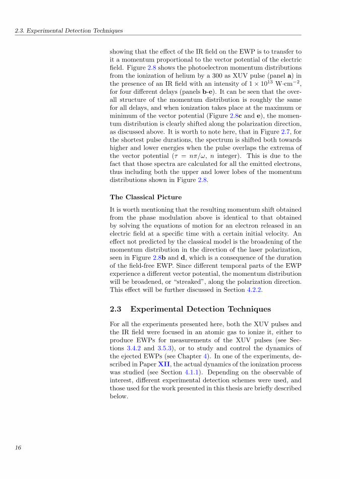
Figure 2.8. Electron momentum distributions from helium ionized bya 300 as XUV pulse in the presence of an IR field. The XUV pulsehas a central energy of 39 eV and the IR intensity is 1× 10¹³ W·cm−2.Above the momentum maps the delay between the XUV pulses (blackline) and the vector potential of the IR field (gray line) is indicated.
2.2.2 Sub-Cycle Ionization
Both the ponderomotive shift and the generation of sidebands areeffects of averaging over several IR cycles, and are thus not sen-sitive to delay changes on the sub-cycle time-scale between theXUV pulses and the IR field. In Figure 2.7 calculated photoelec-tron spectra are shown as a function of the delay, τ , between theIR field cycle and the XUV pulse, for decreasing XUV pulse du-rations and an IR intensity of 1 × 10¹² W·cm−2. Also for thesecalculations, the IR field amplitude is constant over the durationof the XUV pulse. It can be seen that as the XUV pulse durationdecreases, the width of the photoelectron peaks increases, and asit becomes close to or shorter than half the period of the IR laserfield (1.3 fs), delay-dependent effects appear. For XUV pulse dura-tions significantly shorter than the IR period, clear oscillations athigh and low energies are seen, with maximum energy shifts at thezero-crossings of the electric field, corresponding to the extrema ofthe vector potential (τ = nπ/ω, n integer).
Momentum Shift
When the XUV pulse is very short compared with the period ofthe phase modulation, φIR (pf , t), the phase accumulated by theEWP varies almost linearly with time, such that the main effectof the laser is to introduce an energy shift, ∆W , given by:
∆W =p2
f (t)− p20
2m= −h
∂φIR (pf , t)∂t
(2.16)
where p0 is the initial momentum. Using Equation (2.7), this canbe solved to give:
pf (t) = p0 − eA (t) (2.17)
15
2.3. Experimental Detection Techniques
showing that the effect of the IR field on the EWP is to transfer toit a momentum proportional to the vector potential of the electricfield. Figure 2.8 shows the photoelectron momentum distributionsfrom the ionization of helium by a 300 as XUV pulse (panel a) inthe presence of an IR field with an intensity of 1× 10¹³ W·cm−2,for four different delays (panels b-e). It can be seen that the over-all structure of the momentum distribution is roughly the samefor all delays, and when ionization takes place at the maximum orminimum of the vector potential (Figure 2.8c and e), the momen-tum distribution is clearly shifted along the polarization direction,as discussed above. It is worth to note here, that in Figure 2.7, forthe shortest pulse durations, the spectrum is shifted both towardshigher and lower energies when the pulse overlaps the extrema ofthe vector potential (τ = nπ/ω, n integer). This is due to thefact that those spectra are calculated for all the emitted electrons,thus including both the upper and lower lobes of the momentumdistributions shown in Figure 2.8.
The Classical Picture
It is worth mentioning that the resulting momentum shift obtainedfrom the phase modulation above is identical to that obtainedby solving the equations of motion for an electron released in anelectric field at a specific time with a certain initial velocity. Aneffect not predicted by the classical model is the broadening of themomentum distribution in the direction of the laser polarization,seen in Figure 2.8b and d, which is a consequence of the durationof the field-free EWP. Since different temporal parts of the EWPexperience a different vector potential, the momentum distributionwill be broadened, or “streaked”, along the polarization direction.This effect will be further discussed in Section 4.2.2.
2.3 Experimental Detection Techniques
For all the experiments presented here, both the XUV pulses andthe IR field were focused in an atomic gas to ionize it, either toproduce EWPs for measurements of the XUV pulses (see Sec-tions 3.4.2 and 3.5.3), or to study and control the dynamics ofthe ejected EWPs (see Chapter 4). In one of the experiments, de-scribed in Paper XII, the actual dynamics of the ionization processwas studied (see Section 4.1.1). Depending on the observable ofinterest, different experimental detection schemes were used, andthose used for the work presented in this thesis are briefly describedbelow.
16

Photoionization Using Extreme Ultraviolet Pulses
+Vacc
Ground
Field-free
flight tube
Detector
Figure 2.9. Schematic of an iontime-of-flight spectrometer.
2.3.1 Ion Time-of-Flight Spectrometer
An ion time-of-flight (TOF) spectrometer is used for the detectionof ions, separating them according to their charge and mass. Asdepicted in Figure 2.9, ionization takes place in between two elec-trodes, one which is grounded and has a hole in the center, andone which has a high positive voltage (Vacc ∼ 1 kV) applied to it.The created ions are accelerated by the static electric field, travelthrough the field-free flight tube, in the end of which they are de-tected using, for example, an electron multiplier tube. The timeof arrival is inversely proportional to the velocity of the ion whenit enters the field-free region (apart from a small correction due tothe acceleration time), which in turn is proportional to the squareroot of the ratio between the charge and the mass of the ion. Byrecording the time dependence of the signal from the detector us-ing, for example, an oscilloscope, ions with different charge-massratios can be separated, and their abundance quantified. In theexperiment presented in Paper XII, the VMIS, described below,was used as an ion TOF spectrometer.
2.3.2 Magnetic Bottle Electron Spectrometer
The MBES is also based on the TOF technique, but instead ofdetecting ions according to their charge and mass, it measures thekinetic energies of the electrons created in the ionization, i.e. thephotoelectron spectrum. Thus, no extraction field is used, sincethe observable of interest is the initial velocity of the electrons. Inthe MBES, ionization takes place in a region with a strong mag-netic field (∼ 1 T), which is parallel to the flight tube direction.The field adiabatically decreases towards the flight tube, where itis constant (∼ 1 mT). The ejected electrons will spiralize aroundthe magnetic field lines, and as the field gets weaker, the initialvelocity of the electrons will gradually be converted into longitu-dinal velocity, i.e. a velocity in the direction of the flight tube [40].By using this magnetic bottle, all electrons that initially have avelocity component in the direction of the flight tube, will eventu-ally reach the detector, implying a theoretical collection efficiencyof 50%. The detector used is a microchannel plate (MCP), fromwhich a signal, corresponding to the total electron count over thedetector area, is collected using a multi-scaler computer card. Af-ter performing a calibration to determine the relation between theTOF and the photoelectron energy, the photoelectron spectrumcan be calculated from the recorded detector signal. For the injec-tion of the target gas, the experiments presented here have used astatic gas pressure of ∼ 10−4 mbar. The MBES was used for theexperiments presented in Papers I-VI, VIII, X and XI.
17

2.3.3. Velocity Map Imaging Spectrometer
Repeller
Extractor
Ground
VR
VE
0
MCPs
Phosphor screen
SkimmerPulsedgas jet
x
z
y
Figure 2.10. Schematic of thevelocity map imagingspectrometer
x (pixels)
y(p
ixel
s)
a
0 100 2000
100
200
px (10−24 Ns)
py
(10−
24N
s)
b
-1 0 1-1
0
1
Figure 2.11. Velocity map imagedata for electrons from heliumionized by an XUV pulse with acentral energy of 26 eV. a, rawimage, 2D projection of the 3Ddistribution, b, image afterinversion, 2D section through the3D distribution.
2.3.3 Velocity Map Imaging Spectrometer
The principle of the VMIS is very different from the two spectrom-eters described above. Instead of measuring the flight time of theelectron, it measures its transverse momentum3. In Figure 2.10, aschematic picture of the VMIS is shown. To obtain high-qualityimages, it is important that the electrons are created only froma small volume, and thus the focused light beam is crossed witha pulsed atomic beam. This is obtained by sending a pulse ofgas from a gas jet through a skimmer, blocking all but a centralcollimated beam of gas. The ionization takes place between twoelectrodes, the extractor and the repeller, with applied potentialsVR < VE < 0. The voltages are in the order of kilovolts, leading toa strong acceleration of the electrons in the z-direction, towards thedetector, which consists of imaging MCPs coupled to a phosphorscreen. The impact coordinates (x, y) on the detector of electronsoriginating from a given point in the interaction volume, reflecttheir initial transverse momentum (i.e. in the xy-plane). Further,by properly choosing the ratio VR/VE, it is possible to obtain focus-ing of the electrons, so that all electrons in the interaction volumewith the same initial momentum, end up at the same coordinateson the detector [41]. Thus, what is measured with a VMIS, is the2D projection of the 3D momentum distribution of the electrons.
Image Acquisition and Inversion
In the experiment, a charge-coupled device (CCD) camera is usedto image the phosphor screen, and the images are transferred toa computer for storage and analysis. An example of such a CCD-image is shown in Figure 2.11a, obtained from ionization of heliumusing an XUV pulse with a central energy of 26 eV. To be ableto reconstruct the full 3D momentum distribution, it is necessaryto use the fact that the distributions are rotationally symmetricaround the polarization direction of the XUV field, which for allcases discussed in this thesis correspond to the y-axis. The ini-tial distribution can then in principle be recovered by Abel inver-sion [42]. However, this method does not perform very well onexperimental data, so for the experiments presented here, an iter-ative inversion procedure has been used [43]. The result of suchan inversion can be seen in Figure 2.11b, showing a 2D sectionthrough the 3D photoelectron distribution, obtained from the 2Dprojection shown in panel a.
The VMIS was used to measure electron momentum distribu-tions in the experiments presented in Papers XII-XIV. In addi-tion, it can be used in ion TOF mode. In that case, VR > 0 and
3It can be noted that velocity map imaging works equally well for ions,using different voltage settings. In this thesis however, only electron imagingdata are presented.
18

Photoionization Using Extreme Ultraviolet Pulses
VE = 0, and instead of images, the total signal from the phosphorscreen is recorded as a function of time. This feature was used forthe experiments presented in Paper XII.
19


x
W
V0
Figure 3.1. Step one: the electrontunnels through the potentialbarrier which is suppressed by thelaser field. The dashed curveshows the unperturbed potential.
x
W
-
Figure 3.2. Step two: the electronis accelerated in the electric field,gaining kinetic energy, W . Thedashed curve shows the shape ofthe potential at the time oftunneling.
Chapter 3
Extreme Ultraviolet OpticalWave Packets
The XUV optical wave packets that are generated in the interac-tion between strong femtosecond laser pulses and atoms, have fea-tures both on the femtosecond and attosecond time-scales. On thefemtosecond time-scale, they are conveniently described as high-order harmonics of the driving frequency, while on the attosecondtime-scale, the picture of re-colliding EWPs, emitting short burtsof XUV radiation every half-cycle of the driving field, is more ap-propriate.
This chapter starts from the sub-cycle picture, first detailing asemi-classical model describing the emission, and then introducinga quantum mechanical model, comparing some results of the two.It moves on to a short presentation of some experimental aspectsof the XUV generation process, including a description of the lasersystem used for the experiments presented in this thesis. Finally,the experiments presented in Papers I-IX are overviewed.
3.1 The Semi-Classical Model
The generation of attosecond XUV pulses from atoms interactingwith a strong laser field can be conveniently explained and under-stood through the so-called three-step model, suggested in 1993 toexplain the dynamics behind the generation of high-order harmon-ics [5–7].
In the first step, an atom exposed to the strong laser field isionized at a certain time by tunneling of the outermost electronthrough the potential barrier formed by the atomic potential andthe electric field, as shown in Figure 3.1. In the second step, theelectron is regarded as a classical particle starting with zero kineticenergy in the electric field at the time of ionization. The motion of
21

3.1.1. Electron Trajectories
Ele
ctric
field
(E0)
-1
0
1
Time, ωt (rad)
Ele
ctro
npos
itio
n(
eE0
mω
2)
ωti = 0.4π
ωti = 0.55π
ωti = 0.7π
0 π 2π 3π 4π 5π 6π-6
-3
0
3
6
Figure 3.4. Classical electron trajectories for three different ionizationtimes (black lines). The electric field is illustrated as the sinusoidalcurve and the instants of ionization are indicated by black dots.
the electron is considered to be governed completely by the laserfield, and the electron can gain or loose energy as it oscillates in theelectric field, as shown in Figure 3.2. For some ionization times, theelectron will return to its parent ion, where it may recombine. Inthis recombination process the excess energy, including the bindingenergy of the final state, is converted into and emitted as a photon,as shown in Figure 3.3.
x
W
γ
Figure 3.3. Step three: theelectron has been turned aroundby the laser field and returns tothe atom (x = 0), where itrecombines and emits its energyas a photon, γ.
3.1.1 Electron Trajectories
The trajectory of an ionized electron is determined by the time oftunneling. For a laser field described by E (t) = E0 sin (ωt), theposition of an electron ionized at time ti is given by:
x (t) =eE0
mω2[sin (ωt)− sin (ωti)− ω (t− ti) cos (ωti)] (3.1)
where e and m are the charge and mass of the electron. Figure 3.4shows the electric field and the position of the ionized electronfor three different times of ionization. It can be seen that forωti = 0.4π the electron is accelerated away from the ion core,while for the other two ionization times it passes the ion once(ωti = 0.7π), and three times (ωti = 0.55π).
A more detailed analysis of Equation (3.1) for the first half-cycle of the electric field shows that only electrons ejected at timesπ2 ≤ ωti < π will return to the core to recombine1. In the toppanel of Figure 3.5 the distance between the ejected electron andthe ion is shown on a grayscale as a function of the ionization time,ti, and time, t. The dashed line indicates the times at which theelectron passes the ion. As can be seen, all electrons ejected in the
1Note that it is sufficient to consider one half-cycle of the field, since theonly thing that differs between the two half-cycles is the sign of the electroncoordinate.
22

Extreme Ultraviolet Optical Wave Packets
Dis
tanc
efr
omio
n(
eE0
mω
2)
0
5
10
Ioni
zation
tim
e,ωt i
(rad
)
0
π
Time, ωt (rad)
Ret
urn
ener
gy(U
P)
0 π 2π 3π 4π 5π 6π 7π 8π 9π 10π0
1
2
3
Figure 3.5. Classical re-collision events. The top panel shows the dis-tance between the electron and the ion for ionization events taking placeduring one half-cycle of the laser field. The dashed line indicates thetimes for which the electron returns to the core, while the bottom panelshows the energy of the returning electron at these instants.
time range π2 ≤ ωt < π re-collide at least once, while the electrons
ejected close to the peak of the field (ωt = π2 ) experience several
collision events.The kinetic energy of the electron in the electric field is given
by:
W (t) = 2UP [cos (t)− cos (ti)]2 (3.2)
where UP = e2E20
4mω2 is the ponderomotive energy, corresponding tothe wiggling energy of an electron in an electric field. In the bot-tom panel of Figure 3.5 the return energy of the electron at thedifferent re-collision events is plotted. It can be seen that the gen-eral structure of all the re-collisions is the same, beginning withlow-energy electrons, increasing towards a maximum in re-collisionenergy and finally decreasing again. The maximum return energyis highest for the first re-collision, and then asymptotically ap-proaches a value of ≈ 2UP. In practice, the contributions from thehigher-order returns are very weak, due to the long time the elec-tron spends in the continuum in combination with phase-matchingeffects [44].
23

3.1.2. Classical Predictions
Time, ωt (rad)
Ret
urn
ener
gy
(UP)
π 3π2
2π 5π2
0
1
2
3
Exc
urs
ion
tim
e,ω
(t−
t i)(
rad)
0
2
4
6
Figure 3.6. Details of the firstre-collision event. The solid lineshows the return energy and thedashed line the time spent by theelectron in the continuum. Thedash-dotted lines show theposition of the classical cut-off.
3.1.2 Classical Predictions
Although the semi-classical model is a simple one, it has beenshown to predict many features of the XUV emission from an atomin a strong field. Focusing here on the first re-collision, the energyof the returning electron (solid line) and the excursion time t− ti(dashed line), i.e. the time spent by the electron in the continuum,are plotted as a function of time in Figure 3.6.
The first observation, as can also be seen in Figure 3.5, is thatthe maximum in the return energy occurs for electrons returningat ωt ≈ 6 rad, slighty before the zero-crossing of the electric field.These electrons will have an energy of 3.2 UP, and this is themaximum classical return energy that any electron can have whenreturning to the ion. For the emitted photons, this confirms theso-called cut-off law predicted empirically by Krause et al. [45],stating that the maximum photon energy scales as ECO = Ip +3.2UP, where Ip is the ionization energy of the atom.
For all but the cut-off electrons, it can be seen in Figure 3.6 thatthere are always two trajectories returning with the same energy.These can be assigned to two different branches, those returningbefore the cut-off electrons and those returning after. Due to thetime the electrons belonging to the different branches spend in thecontinuum, these are often referred to as the short and the longtrajectory2.
From the existence of two types of trajectories one can inferthat, for XUV radiation with a certain bandwidth and with a cen-tral energy below the cut-off energy, there will be two bursts ofradiation during each half-cycle of the driving field. Furthermore,the pulses emitted will not be transform-limited since, according toFigure 3.6, the energies are spread out in time (see Section 1.3.2).In particular, the pulses arising from the short trajectory shouldhave a positive chirp, while the chirp of the long trajectory pulsesshould be negative, predictions that have recently been experimen-tally confirmed [46, 47], and will be further discussed in Section 3.5.
3.2 The Quantum Picture
The semi-classical model provides considerable insight into the dy-namics of an atom in a strong laser field and is able to shed somelight on many of the results obtained experimentally. However,in the real world, there is no electron taking a trip in the contin-uum and later returning to the core, but rather part of a boundelectron wave packet, tunneling through the classically forbiddenpotential barrier, propagating in the continuum in the presenceof the atomic potential and finally interfering with the part of it
2In the literature one often sees the notations first and second trajectory,or τ1 and τ2 for the short and long trajectories, respectively. The reason forthis will become clear in Section 3.2.4
24

Extreme Ultraviolet Optical Wave Packets
Ellipticity, ε
Effi
cien
cy(a
rb.
u.)
-0.4 -0.2 0 0.2 0.410−3
10−2
10−1
100
Figure 3.7. Ellipticity dependenceof the XUV conversion efficiency.
Intensity (arb. u.)
10−2 10−1
Time (as)
Photo
nen
ergy
(eV)
-1000 0 1000
20
30
40
50
Figure 3.8. Visualization of thesingle-atom emission from argonatoms subjected to an 800 nmlaser field with an intensity of1.4× 1014 W·cm−2, calculated byintegration of the TDSE followedby a wavelet analysis. The solidwhite lines show the predictedreturn times and energiesobtained using the semi-classicalmodel for the first two returns ofthe electron.
that is left in the bound states of the atom. Thus, effects thatcannot be described classically come into play, such as the accu-mulation of phase due to the tunneling and the presence of theCoulomb potential, and the spatial spreading of the wave packetas it propagates in the continuum.
3.2.1 Ellipticity Dependence
A clear manifestation of the quantum nature of the electron contin-uum dynamics is the dependence of the XUV conversion efficiencyon the polarization of the generating field [48–50]. According tothe semi-classical model, photon emission would cease completelyas soon as a small amount of ellipticity is introduced, since it isthen impossible for the electron to return to the ion core to re-combine. In the quantum picture, however, one has to include thetransverse spread of the wave packet in the continuum, resulting ina certain probability of recombination also for elliptical polariza-tion. Figure 3.7 shows the XUV conversion efficiency as a functionof ellipticity3, ε, using a perturbative model [49] fitted to experi-mental results [48]. This model was applied in Paper V where theellipticity dependence is used to achieve temporal confinement ofthe XUV emission (see Section 3.4.4).
3.2.2 The Full Calculation
To obtain the full picture it is necessary to solve the time-dependent Schrodinger equation (TDSE) for the system consist-ing of the atom and the laser field [51]. In Figure 3.8 the resultsof such a calculation are presented for an argon atom exposedto an IR field with a wavelength of 800 nm and an intensity of1.4× 1014 W·cm−2. What is shown is the distribution of emissionfrequencies as a function of time, obtained via a wavelet analy-sis [52]. The picture reveals a complicated time structure, repeat-ing itself with half the period of the driving field (1330 as). As willbe discussed below, this repetition is what gives rise to the discreteharmonic peaks. During a single half-cycle, for a given range ofenergies there are multiple bursts of radiation, in qualitative agree-ment with the semi-classical model, whose return times and ener-gies are shown for comparison for the first two re-collisions. It canbe seen that the two dominating contributions to the emission seemto come from the short trajectories of both re-collisions, a behav-ior that has previously been reported as typical for emission fromargon [53]. Quantitatively, the agreement with the semi-classicalmodel is not that obvious, which is not surprising considering itssimplicity. It has, however, been shown that for conditions closer
3The ellipticity denotes the ratio of the amplitudes of two perpendicularcomponents of the electric field, such that ε = 0 and ε = 1 correspond to linearand circular polarization, respectively.
25

3.2.3. The Strong-Field Approximation
to those under which the semi-classical model is derived (longerwavelengths and higher intensities), the quantitative agreementgets significantly better [54].
3.2.3 The Strong-Field Approximation
Although possible, the full calculation is demanding in terms ofcomputer power and is also increasingly time consuming with thelevel of complexity of the studied system. In addition, if the aimis to obtain some understanding of the process, the results of afull calculation may be very difficult to interpret, as exemplifiedby the distribution in Figure 3.8. A very successful, fully quantummechanical, approach to the problem was formulated shortly afterthe semi-classical model was proposed [8, 9]. As for the two-colorionization model, introduced in Section 2.2, the derivation is basedon a strong-field approximation (SFA) of the Schrodinger equation,neglecting the influence of the atomic potential on the electron inthe continuum, as well as the influence of all bound states exceptthe ground state. For studying the emission from the atom, thequantity of interest is the time-dependent dipole moment4, givenby:
D (t) = −i
∫ t
−∞dt′
∫d3p d [p + eA (t′)] ·E (t′)
× exp [iφ (p, t′, t)]× d∗ [p + eA (t)] (3.3)
where E (t) and A (t) are the electric field and vector potential,respectively, and d (p) is the dipole matrix element for the transi-tion from the ground state to the continuum state with momentump (∗ denotes complex conjugation). Equation (3.3) clearly illus-trates the classical picture discussed above, with the electron beingionized at time t′ and recombining with the ion at time t. In be-tween these times, the electron accumulates a phase relative to theground state of the atom, given by:
φ (p, t′, t) = − 1h
∫ t
t′dt′′
[p + eA (t′′)]2
2m+ IP
(3.4)
where IP is the ionization potential of the atom. The two integralsaccount for the fact that the dipole moment at time t is the sumof contributions from electrons ionized at all earlier times, t′ < t,and over all possible electron momenta, p.
The Dipole Spectrum
In the following, a linearly polarized, monochromatic laser fieldwith frequency ω, i.e. E (t) = E0 sin (ωt), is assumed. As in the
4Since the emission strength is proportional to the square of the dipoleacceleration.
26

Extreme Ultraviolet Optical Wave Packets
Emission intensity (arb. u.)10−30 10−20 10−10
Photon energy, hΩ (eV)
IRin
tens
ity,
I(W
·cm−
2)
a
10 20 30 40
1013
1014
Emission intensity (arb. u.)10−15 10−10 10−5
Photon energy, hΩ (eV)
b20 40 60
Figure 3.9. Emission intensity,∣∣Ω2D (Ω, I)
∣∣2, as a function of photon
energy and IR intensity, calculated using the SFA (a) and by integra-tion of the TDSE (b). The solid white lines show the cut-off positionpredicted by the classical cut-off law.
classical discussion above, only the emission from a single half-cycleof the electric field is considered, and the frequency spectrum ofthe time-dependent dipole moment in Equation (3.3) can then bewritten:
D (Ω, I) = −i
∫ πω
0
dt
∫ t
−∞dt′
∫d3p d [p + eA (t′)] ·E (t′)
× exp i [φ (p, t′, t) + Ωt] × d∗ [p + eA (t)] (3.5)
where Ω corresponds to the frequency of the emitted radiation andI = 1
2ε0c |E0|2 is the intensity of the driving field.In Figure 3.9, the emission intensity,
∣∣Ω2D (Ω, I)∣∣2, is shown
as a function of photon energy and IR intensity, calculated usingthe SFA (panel a) and by integration of the TDSE (panel b). Ascan be seen, the qualitative agreement between the two is good,showing the perturbative region at low energies, with an intensityrapidly decaying with energy. For sufficiently high intensities, thisis followed by the plateau, leading to a cut-off. The cut-off energy isseen to increase with intensity, in fair agreement with the classicalcut-off law, ECO = IP + 3.2UP, shown by the solid white lines.In the plateau region, ripples can be seen in the dipole emissionintensity as the IR intensity is varied. As discussed below, theseare the result of interference between different quantum orbits.
27

3.2.4. Quantum Orbits
3.2.4 Quantum Orbits
From Equation (3.5) it can be seen that for each frequency compo-nent, there are an infinite number of contributions to the integral.Although numerically more tractable than solving the full TDSE,in this form the SFA model hardly reveals any more informationabout the process. In practice, for high laser intensities only alimited number of paths contribute significantly to the emission.These contributions arise from the quantum orbits, pn, t′n, tn,for which the phase term in Equation (3.5), φ (p, t′, t) + Ωt, is sta-tionary. The quantum orbits are normally indexed according tothe time τ the electron spends in the continuum, τn = tn − t′n, sothis increases with n. Thus, it is common to refer to the differentquantum orbits as τ1, τ2, etc.
As shown by Lewenstein et al. [55], the quantum orbits canbe found using a saddle-point approximation of the integrals inEquation (3.5). Including the result that, for a linearly polarizeddriving field, the resulting dipole will be polarized parallel to thepolarization of the field [55], Equation (3.5) can be rewritten as:
D (Ω, I) =∑
n
Dn (Ω, I) (3.6)
where the sum extends over all relevant quantum orbits. Thus,as in the semi-classical model, it is also possible to separate thecontributions from different trajectories in the quantum picture,using the saddle-point solutions to the SFA. However, a very im-portant difference from the semi-classical model is illustrated bythe coherent sum in Equation (3.6), where, for a given frequency Ω,the total emission will be determined by interfering contributionsfrom the different quantum orbits.
3.2.5 The Dipole Amplitude and Phase
As can be seen above, each quantum orbit, τn, contributes a termDn (Ω, I) to the sum in Equation (3.6), which is usually writtenas:
Dn (Ω, I) = An (Ω, I) exp [iΦn (Ω, I)] (3.7)
where An and Φn are the dipole amplitude and phase, respectively.For the components in the plateau, the dipole amplitude is onlyweakly dependent on intensity and energy, and thus does not sig-nificantly influence the temporal structure of the emission. Thedipole phase, on the other hand, will have a considerable impacton the temporal structure, and for reasons that will become clearlater, it is useful to consider its dependence on energy and intensityseparately.
28

Extreme Ultraviolet Optical Wave Packets
Emission time, te (as)
Photo
nen
ergy,
hΩ
(eV)
τ1 τ2
-1000 -500 0 500
20
30
40
50
60
Figure 3.10. Comparison betweenthe emission times for thequantum orbits obtained from theSFA (solid lines) and the classicalreturn time (dashed line). Thecalculations are done for the IRintensities 1× 10¹⁴ W·cm−2 (thinlines) and 2× 10¹⁴ W·cm−2
(thick lines).
Photon energy, hΩ (eV)
αn
(10−
14W−
1·c
m2)
τ1
τ2
20 40 600
10
20
Figure 3.11. Intensity dependenceof the first two quantum pathsillustrated by the linearityconstant αn, plotted as a functionof the emission energy for the IRintensities 1.5× 10¹⁴ W·cm−2
(thin lines) and 2× 10¹⁴ W·cm−2
(thick lines).
Energy Dependence
The sub-cycle structure of the emission will be determined by thevariation in the dipole phase with energy at a constant intensity.It is useful to define the emission time:
te,n (Ω, I) =∂Φn (Ω, I)
∂Ω(3.8)
which is the group delay of the frequency components of τn cen-tered around Ω (see Section 1.3.2). It can be shown [46] that theemission time is equal to the real part5 of the recombination time,i.e. te,n (Ω) = Re tn (Ω). In Figure 3.10 the emission energy hΩis plotted versus the emission time for the two shortest quantumorbits, τ1 and τ2, using IR intensities of 1 × 10¹⁴ W·cm−2 (thinlines) and 2× 10¹⁴ W·cm−2 (thick lines). As can be seen, the SFAresults clearly reflect the semi-classical nature of the emission pro-cess, showing good qualitative agreement with the purely classicalresult from Figure 3.6, shown by the dashed line. Quantitatively,the tunneling process results in corrections to the emission energiesand also replaces the sharp classical cut-off by a smooth mergingof the two quantum orbits.
Intensity Dependence
When it comes to effects appearing on the time-scale of the drivinglaser pulse duration, the dependence of the dipole phase on inten-sity becomes important. As can be seen in Figure 1 of Paper VIII,in the plateau the dipole phase has an almost linear dependenceon the intensity, and it is thus common to introduce a linearityconstant, αn:
αn (Ω, I) = −∂Φn (Ω, I)∂I
(3.9)
In Figure 3.11 this is plotted as a function of the emission en-ergy for the IR intensities 1.5 × 10¹⁴ W·cm−2 (thin lines) and2× 1014 W·cm−2 (thick lines). It can be seen that while α1 has avalue close to zero, positive for all but the lowest harmonics, thevalue of α2 is larger, indicating that τ2 is more sensitive to inten-sity variations. Classically, this can be explained by the longertime the electrons belonging to τ2 spend in the continuum, thusbeing more strongly affected by the IR field.
5Interestingly, the resulting times t′n and tn are in general complex quanti-ties, with an imaginary part that can be attributed to the tunneling involved.
29
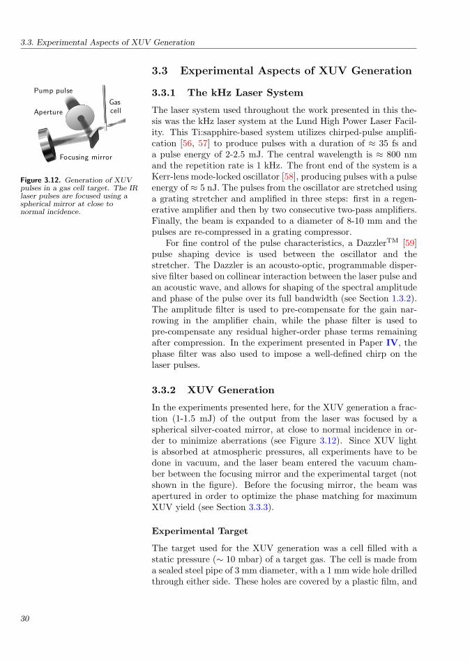
3.3. Experimental Aspects of XUV Generation
Pump pulse
Aperture
Focusing mirror
Gascell
Figure 3.12. Generation of XUVpulses in a gas cell target. The IRlaser pulses are focused using aspherical mirror at close tonormal incidence.
3.3 Experimental Aspects of XUV Generation
3.3.1 The kHz Laser System
The laser system used throughout the work presented in this the-sis was the kHz laser system at the Lund High Power Laser Facil-ity. This Ti:sapphire-based system utilizes chirped-pulse amplifi-cation [56, 57] to produce pulses with a duration of ≈ 35 fs anda pulse energy of 2-2.5 mJ. The central wavelength is ≈ 800 nmand the repetition rate is 1 kHz. The front end of the system is aKerr-lens mode-locked oscillator [58], producing pulses with a pulseenergy of ≈ 5 nJ. The pulses from the oscillator are stretched usinga grating stretcher and amplified in three steps: first in a regen-erative amplifier and then by two consecutive two-pass amplifiers.Finally, the beam is expanded to a diameter of 8-10 mm and thepulses are re-compressed in a grating compressor.
For fine control of the pulse characteristics, a DazzlerTM [59]pulse shaping device is used between the oscillator and thestretcher. The Dazzler is an acousto-optic, programmable disper-sive filter based on collinear interaction between the laser pulse andan acoustic wave, and allows for shaping of the spectral amplitudeand phase of the pulse over its full bandwidth (see Section 1.3.2).The amplitude filter is used to pre-compensate for the gain nar-rowing in the amplifier chain, while the phase filter is used topre-compensate any residual higher-order phase terms remainingafter compression. In the experiment presented in Paper IV, thephase filter was also used to impose a well-defined chirp on thelaser pulses.
3.3.2 XUV Generation
In the experiments presented here, for the XUV generation a frac-tion (1-1.5 mJ) of the output from the laser was focused by aspherical silver-coated mirror, at close to normal incidence in or-der to minimize aberrations (see Figure 3.12). Since XUV lightis absorbed at atmospheric pressures, all experiments have to bedone in vacuum, and the laser beam entered the vacuum cham-ber between the focusing mirror and the experimental target (notshown in the figure). Before the focusing mirror, the beam wasapertured in order to optimize the phase matching for maximumXUV yield (see Section 3.3.3).
Experimental Target
The target used for the XUV generation was a cell filled with astatic pressure (∼ 10 mbar) of a target gas. The cell is made froma sealed steel pipe of 3 mm diameter, with a 1 mm wide hole drilledthrough either side. These holes are covered by a plastic film, and
30

Extreme Ultraviolet Optical Wave Packets
the laser beam is used to drill a small hole through this, thus mini-mizing the leakage of gas from the cell to the surrounding vacuum,making it easier to maintain a low pressure in the chamber.
Choice of Non-Linear Medium
The choice of the non-linear medium for the XUV generation is atrade-off between conversion efficiency and maximum photon en-ergy. The conversion efficiency is closely linked to the polarizabilityof the medium, while the maximum photon energy depends on theionization potential, partly due to the IP term in the expression forthe classical cut-off (see Section 3.1.2), but mainly since a higherionization potential means that the medium can be exposed to ahigher intensity before being ionized.
A high ionization potential means strongly bound electrons,and thus a low polarizability. Taking the rare gases as examples,the lightest gases, helium and neon, have high ionization poten-tials but low polarizability, leading to high photon energies, butrather poor conversion efficiency. For the heavier elements, likekrypton and xenon, the situation is reversed, and the emission ex-hibits higher XUV intensities, but only at low photon energies. Inthe experiments presented in this thesis, mainly argon has beenused for the XUV generation. In Paper XII, however, xenon wasused as the generating gas, since for this experiment low photonenergies were required (≈ 20 eV), as discussed in Section 4.1.1. Ina recent experiment performed in Lund, where large XUV band-widths were required, neon was used as a generating gas, resultingin a maximum photon energy above 100 eV [60].
3.3.3 Macroscopic Effects
Thus far, the discussion has only dealt with the response of a sin-gle atom to a strong laser field, and has detailed how this leads tobursts of XUV radiation with certain spectral profiles and phasesdepending on the specific quantum orbit responsible for the emis-sion. In practice, XUV generation takes place in a medium con-sisting of many atoms or molecules, with a certain density profile,subjected to a laser field with a spatial and longitudinal intensitydistribution. All of these sources radiate in all directions, with am-plitudes and phases depending on the local IR intensity, and theresulting XUV emission is the coherent sum of these contributions.For example, the directionality, i.e. the fact that the XUV radia-tion emerges collinearly with the generating beam, is the result ofinterference between radiation from the different atoms, adding upconstructively only in the forward direction. Much theoretical andexperimental effort has been devoted to investigating these macro-scopic effects [55, 61–65]. The work presented here has mainlybeen concerned with the single-atom aspects, and only a few ef-
31

3.4. Femtosecond High-Order Harmonics
fects, essential for the understanding of the results in this thesis,are considered below.
Effects of Phase Matching
The XUV emission is optimized when the contributions from dif-ferent points along the medium length are in phase. There are es-sentially three effects that can cause a phase mismatch: the Gouyphase shift of π that a laser beam experiences when it goes througha focus; dispersion (see Section 1.3.2), dominated by the disper-sion of free electrons created by ionization and the dipole phase,which varies with intensity over the medium, as discussed in Sec-tion 3.2.5. The total phase mismatch will be determined by theinterplay between these effects, and will depend on: the pressure ofthe target gas, the intensity, the focusing conditions, the mediumlength and the position of the laser focus in relation to the medium.
Using loose focusing minimizes the phase mismatch due to theGouy phase shift and the dipole phase variation, while keeping theintensity low will lead to less ionization and thus minimize the mis-match due to dispersion of free electrons. In addition, by focusingthe laser before the medium, it is possible to find a situation wherethe phase mismatch from the dipole phase partly cancels out thatcaused by the Gouy phase shift, so that good phase matching isobtained on the optical axis for the short quantum orbit [55, 63].
Spatial Profiles
The intensity dependence of the dipole phase, quantified by thelinearity constant αn in Section 3.2.5, also has consequences forthe spatial properties of the XUV emission. From a typical spatialprofile, two regions can be identified: a central part, consisting ofcontributions from the first quantum orbit; and a more divergentpart, containing emission from the second quantum orbit [66]. Thedifference in divergence is caused by the transverse variation of thelaser intensity over the focus, leading to a curvature of the XUVwave fronts, with a magnitude that scales with αn. As discussedin Section 3.2.5 (see also Figure 3.11), α2 > α1, so that the wavefront of the emission from the second quantum orbit has a largercurvature, and is thus more divergent than the emission from thefirst quantum orbit. As will be further discussed in Sections 3.4.3and 3.5.1, this difference in divergence between emission from dif-ferent quantum orbits, allows for selection of a single contributionby blocking different parts of the spatial profile.
3.4 Femtosecond High-Order Harmonics
For the experiments presented in this thesis, laser pulses of fem-tosecond duration, corresponding to many laser cycles at the
32
Extreme Ultraviolet Optical Wave Packets
Ti:sapphire wavelength of 800 nm, were used for the generationof XUV radiation. This means that the sub-cycle process dis-cussed above is repeated, so that, instead of a single burst, a trainof bursts is generated. The temporal structure of these trains andthe pulses therein are discussed in Section 3.5, while this sectionwill focus on the temporal structure of the high-order harmonicsthat appear in the spectrum as a result of this repetition.
3.4.1 The Harmonic Spectrum
When calculating the emission spectrum resulting from a multi-cycle driving field, one needs to take into account the differ-ence between two consecutive half-cycles. Equation (3.6) de-fines the dipole spectrum from the first half-cycle of a sinu-soidal driving field, obtained from a saddle-point analysis ofEquation (3.5). It can be deduced that for the second half-cycle, the saddle-point analysis6 will pick out the quantum orbits−pn, t′n + π/ω, tn + π/ω. Assuming an atomic (symmetric) sys-tem, the dipole spectrum from the second half-cycle will be givenby D′ (Ω, I) = −D (Ω, I), i.e. there will be a phase shift of π in theemission between consecutive half-cycles. Thus, the emission spec-trum resulting from a multi-cycle driving field can be expressed as:
E (Ω) =∑
k
(−1)kD (Ω, Ik) eikπ Ω
ω
=∑
n
∑k
An (Ω, Ik)
× exp
i
[Φn (Ω, Ik) + kπ
(Ωω− 1
)](3.10)
where Ik denotes the instantaneous intensity of the driving fieldduring half-cycle k, and the phase term kπ Ω
ω accounts for the delayof half-cycle k.
Constant Intensity
Assuming a driving field of constant intensity, Ik = I0, it canbe seen that, for each separate quantum orbit, constructive inter-ference will occur between contributions from different half-cycleswhen:
(k + 1) π
(Ωω− 1
)= kπ
(Ωω− 1
)+ j · 2π (3.11)
where j is an integer. Simplifying this expression, one obtainsΩ = (2j + 1)ω, showing that the resulting spectrum will contain
6Note that although the saddle-point analysis is used here to support thediscussion, the conclusions made in this section are general, and not limitedto the SFA treatment.
33

3.4.1. The Harmonic Spectrum
Harmonic order
Inte
nsity
1
2
4
8
17 21 25 29 33
Figure 3.13. Harmonic spectrummade up of a Gaussian emissionspectrum repeated for 1, 2, 4 and8 half-cycles of the driving field.
only odd harmonics of the driving laser frequency. Figure 3.13shows their appearance for a Gaussian emission spectrum repeatedfor 1, 2, 4 and 8 half-cycles.
Intensity-Induced Frequency Shift
When considering the more realistic case of a driving field witha time-dependent intensity, the dipole phase Φn (Ω, Ik) must beincluded in the interference criterion, yielding:
Φn (Ωn, Ik+1) + (k + 1)π
(Ωn
ω− 1
)=
Φn (Ωn, Ik) + kπ
(Ωn
ω− 1
)− j · 2π (3.12)
which can be simplified to:
Ωn = (2j + 1)ω − [Φn (Ωn, Ik+1)− Φn (Ωn, Ik)]ω
π(3.13)
with a correction to the frequency of the harmonics7, depending onthe variation of the dipole phase due to the difference in intensitybetween the two half-cycles. Identifying π/ω as half the periodof the driving field, the discrete differential in the correction termcan be approximated by the continuous one.
Ωn = (2j + 1) ω − ∂Φn (Ωn, I)∂t
= (2j + 1) ω − ∂Φn (Ωn, I)∂I
· ∂I
∂t
= (2j + 1) ω + αn (Ωn, I) · ∂I
∂t(3.14)
Thus, the linearity constant αn, as defined in Equation (3.9), de-scribes how the frequency shift scales with the derivative of theintensity. This frequency shift has important effects on both thespectral and the temporal properties of the emitted harmonics.Spectrally, experiments have shown a blueshift of the harmonicfrequencies as a result of ionization [67] since, for high laser intensi-ties, the medium is ionized before the peak of the pulse, so harmon-ics are only generated on the leading edge of the laser pulse, andthus have a frequency shift towards higher energies (αn > 0) [68].Temporally, the intensity-dependent frequency shift results in anintrinsic chirp on the generated harmonics, an effect that will befurther discussed in Section 3.4.3.
7It might be argued that these are no longer harmonics of the driving laserfrequency, which is of course strictly speaking correct. However, in this thesisthey are referred to as harmonics.
34

Extreme Ultraviolet Optical Wave Packets
3.4.2 Time-Frequency Characterization
In order to measure the time-frequency characteristics of ultra-short pulses, it is necessary to have a filter that is non-stationaryin time [69], i.e. it requires some means of selecting different tem-poral portions of the pulse. In the visible or infrared regime, thiscan easily be achieved by the use of a non-linear effect. In theXUV regime it is difficult, not only to find suitable materials, butalso to reach the high intensities required to induce non-linearprocesses. Despite these difficulties, this has been achieved exper-imentally [15–17, 70–72].
In the experiments presented in Papers I, IV and V a differ-ent approach was used, based on converting the femtosecond XUVpulses into EWPs through single-photon ionization, and character-izing the wave packets from which, as pointed out in Section 2.1,the properties of the XUV pulses can be extracted8.
Cross-Correlation Frequency-Resolved Optical Gating
The technique used for the characterization of the high-orderharmonics is a variant of frequency-resolved optical gating(FROG) [73]. FROG is a group of techniques, where a gate, G (t),with a variable delay, τ , is overlapped with the pulse to charac-terize. For each delay, the spectrum is measured, resulting in aspectrogram:
S (ω, τ) =∣∣∣∣∫ +∞
−∞dt G (t) E (t− τ) eiωt
∣∣∣∣2 (3.15)
where E (t) is the field of the pulse. The gate function is usu-ally derived from the pulse itself, like in the simplest case, secondharmonic generation FROG, where G (t) = E (t). For the mea-surements presented here, the gate is an IR probe pulse, with aduration shorter than the XUV pulse, and the measured spectrumis that of the EWPs ejected when the XUV and IR pulses are usedto ionize a gas [74–76]. This variant of FROG, where the gate func-tion is known, is called cross-correlation frequency-resolved opticalgating (XFROG).
As shown in Section 2.2.1, when the IR probe pulse temporallyoverlaps the XUV pulse, sidebands are generated. In addition, us-ing an IR pulse which is shorter than the XUV pulse, sidebands willonly be generated from the temporal part of the XUV pulse thatoverlaps with the probe. The top panel of Figure 3.14 shows anXFROG spectrogram from the experiment presented in Paper IV,
8When measurements are done for single harmonics, the associated band-widths are so narrow that the variation of the atomic dipole phase can beneglected. The cross section needs to be included in the reconstruction onlyif the relative intensities of the harmonics are required.
35
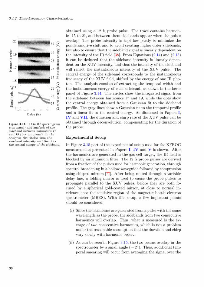
3.4.2. Time-Frequency Characterization
Har
monic
ord
er
15
17
19
21
Photo
elec
tron
ener
gy
(eV)
24
26
28
30
32
Cen
tral
ener
gy
(eV)
27
28
29
Delay (fs)
Sig
nal
(arb
.u.)
-60 -30 0 30 600
1
Figure 3.14. XFROG spectrogram(top panel) and analysis of thesideband between harmonics 17and 19 (bottom panel). In theanalysis, the circles show thesideband intensity and the dotsthe central energy of the sideband.
obtained using a 12 fs probe pulse. The trace contains harmon-ics 15 to 21, and between them sidebands appear when the pulsesoverlap. The probe intensity is kept low partly to minimize theponderomotive shift and to avoid creating higher order sidebands,but also to ensure that the sideband signal is linearly dependent onthe intensity of the IR field [38]. From Equations (2.14) and (2.15)it can be deduced that the sideband intensity is linearly depen-dent on the XUV intensity, and thus the intensity of the sidebandwill reflect the instantaneous intensity of the XUV pulse. Thecentral energy of the sideband corresponds to the instantaneousfrequency of the XUV field, shifted by the energy of one IR pho-ton. The analysis consists of extracting the temporal width andthe instantaneous energy of each sideband, as shown in the lowerpanel of Figure 3.14. The circles show the integrated signal fromthe sideband between harmonics 17 and 19, while the dots showthe central energy obtained from a Gaussian fit to the sidebandprofile. The gray lines show a Gaussian fit to the temporal profileand a linear fit to the central energy. As discussed in Papers I,IV and VII, the duration and chirp rate of the XUV pulse can beobtained through deconvolution, compensating for the duration ofthe probe.
Experimental Setup
In Figure 3.15 part of the experimental setup used for the XFROGmeasurements presented in Papers I, IV and V is shown. Afterthe harmonics are generated in the gas cell target, the IR field isblocked by an aluminum filter. The 12 fs probe pulses are derivedfrom a fraction of the pulses used for harmonic generation, throughspectral broadening in a hollow waveguide followed by compressionusing chirped mirrors [77]. After being routed through a variabledelay line, a folding mirror is used to cause the probe pulses topropagate parallel to the XUV pulses, before they are both fo-cused by a spherical gold-coated mirror, at close to normal in-cidence, into the sensitive region of the magnetic bottle electronspectrometer (MBES). With this setup, a few important pointsshould be considered:
(i) Since the harmonics are generated from a pulse with the samewavelength as the probe, the sidebands from two consecutiveharmonics will overlap. Thus, what is measured is the av-erage of two consecutive harmonics, which is not a problemunder the reasonable assumption that the duration and chirpvary slowly with harmonic order.
(ii) As can be seen in Figure 3.15, the two beams overlap in thespectrometer by a small angle (∼ 2). Thus, additional tem-poral smearing will occur from averaging the signal over the
36

Extreme Ultraviolet Optical Wave Packets
Harmonicgeneration
XUV + IR
Aluminum filter
XUV
Short IRprobe pulse
Focusing
mirror
MBES
Figure 3.15. Cross-correlation setup used for the XFROG measure-ments.
spatial profile of the pump-probe overlap. This geometricalfactor has to be accounted for in the deconvolution.
(iii) The XUV pulses and the probe pulses have different diver-gence, and thus when being focused with the same optics,the IR is focused slightly before the XUV in the sensitiveregion of the spectrometer. This ensures homogeneous IRintensity over the whole overlap volume.
Finally, it should be mentioned that the geometrical issues ofpoints (ii) and (iii) above will efficiently prevent any interferencebetween the two contributions, discussed in point (i), from be-ing seen in the generated sidebands. As will be described in Sec-tion 3.5.3, such effects are essential when measuring the relativeproperties of different harmonics, rather than the properties of asingle harmonic.
3.4.3 Intrinsic and Imposed Harmonic Chirp
The intensity-dependent frequency shift defined in Equation (3.14)has important consequences for the time-frequency characteristicsof the high-order harmonics. Only the case when ionization is lowwill be considered here, so the influence from free electrons [78] canbe neglected, and in addition, the harmonics are generated mainlyat the peak of the generating pulse. For a Gaussian driving pulsethe intensity derivative close to its peak can be approximated as:
∂I
∂t≈ −8I0 ln 2
τ2· t (3.16)
where I0 is the peak intensity and τ the pulse duration. Thus,the time-dependent frequency of the harmonic of order q = 2j +1,
37

3.4.3. Intrinsic and Imposed Harmonic Chirp
a27
28
29
Photo
elec
tron
ener
gy
(eV)
b27
28
29
Delay (fs)
c
-20 -10 0 10 20
27
28
29
Figure 3.16. Sideband toharmonic 17 generated in argon,calculated including the full field(a), the central spatial part (b)and the annular spatial part (c).The sketches in the top rightcorners show the shape of themasks used in the three cases.
from the quantum orbit n, can be written as:
Ωn,q (t) = q (ω + b1t)− αn (qω, I0) ·8I0 ln 2
τ2· t (3.17)
where b1 is the chirp rate of the driving pulse, which is assumed tobe linearly chirped. It is also assumed that the linearity constant,αn, does not vary significantly within the resulting bandwidth ofthe harmonic. As can be seen, there will be two contributions tothe time-dependent frequency of the harmonic: one from the chirprate of the driving field, and one from the intensity-dependentdipole phase. The resulting harmonic chirp rate can be written as:
bn,q = qb1 − αn (qω, I0) ·8I0 ln 2
τ2(3.18)
stating that the chirp rate of the harmonics is simply q times thatof the generating field, plus a contribution due to the atom which,for a given harmonic, is proportional to the intensity of the drivingpulse, and inversely proportional to the square of its duration.
The Short and the Long Quantum Orbit
Since αn is normally positive, the chirp rate of a harmonic gen-erated by a transform-limited pulse, also called the intrinsic har-monic chirp, is in general negative. In addition, as can be seenin Figure 3.11, for τ2 the value of αn is much larger, predict-ing a larger negative chirp for harmonics belonging to the sec-ond quantum orbit. This is exemplified and confirmed in Fig-ure 3.16, showing XFROG traces for a sideband to harmonic 17generated in argon, probed by a 12 fs IR pulse. The harmonic fieldsused were calculated from numerically solving the Maxwell waveequation in the macroscopic medium [79], using dipole momentsfrom TDSE calculations as the non-linear source term, while theXFROG traces were calculated from these using the SFA modeldescribed in Section 2.2.1, including only the first-order sidebands.Panel a shows the sideband resulting from including the full spa-tial extent of the field in the sideband calculation, while in panelsb and c, calculations using the central and outer spatial parts9 ofthe field, respectively, are shown. As discussed in Section 3.3.3,such spatial selection can be used to separate the contributionsfrom the short and the long quantum orbits. This is confirmed inFigure 3.16, where the hole selects the contribution with a smallnegative chirp, corresponding to τ1, and the mask enhances thecontribution from τ2, with a significantly larger negative chirp.
9The spatial selection is implemented in the calculation by simulating theinsertion of a 1 mm circular hole or a 1 mm circular mask into the beam at apoint 35 cm behind the harmonic generation point.
38

Extreme Ultraviolet Optical Wave Packets
Harmonic order
αn
(10−
14W−
1·c
m2)
τ1
τ2
13 17 21 25 29 330
5
10
15
20
25
Figure 3.17. Comparison betweenexperimentally measured values ofαn and values calculated from thesaddle-point solutions of the SFA,for the two shortest quantumorbits.
Chirp Measurements
In the experiments described in Papers I and IV, the chirp rateswere measured for harmonics 13 to 23 generated in argon andspatially filtered using an aperture, as a function of the chirp rateof the driving field, keeping the peak intensity more or less constantand well below the limit where the effects of ionization start toplay a role. The intrinsic harmonic chirp rates were measured,using a transform-limited fundamental pulse, and from these thevalues of αn were extracted. These were found to agree well withcalculated values for τ1, as shown in Figure 3.17 and in Paper VIII,confirming the spatial selection of contributions from the shortquantum orbit. Finally, by varying the chirp rate of the drivingpulse, it was shown that the chirp is transferred to the harmonics,as predicted by Equation (3.17). In particular, by imposing apositive chirp on the fundamental, it is possible to reach a situationwhere a whole range of harmonics have the same chirp rate, leadingto interesting conclusions about the structure of the attosecondbeating between the harmonics, as will be further discussed inSection 3.5.2.
3.4.4 Temporal Confinement Through EllipticityGating
As discussed in Section 3.2.1, for harmonic generation, the conver-sion efficiency is very strongly dependent on the ellipticity of thedriving field [48–50]. Thus, by using a laser pulse with a varyingellipticity, the harmonic generation will be confined to a tempo-ral window that may be shorter than the one determined by theinstantaneous driving laser intensity. This has been suggested,by Corkum et al. [80], as a method of generating isolated atto-second pulses, an idea that has recently gained experimental sup-port [81]. In previous experiments [82–84], spectral measurementshave indicated the existence of temporal confinement through thebroadening of the individual harmonics. In the experiment pre-sented in Paper V (see also [85–87]), a time-resolved study wasperformed of harmonics 13 to 21 generated in argon using anellipticity-modulated fundamental.
Experimental Technique
To create the required polarization gate, a technique based ontwo quartz quarter-wave plates was used [83, 88], as illustratedin Figure 1 of Paper V. The linearly polarized laser pulse is sentthrough the first plate, which is a thick multi-order plate, withits polarization direction at a 45 angle to the optic axis of theplate. This results in two, time-delayed but partly overlapping,perpendicularly polarized replicas of the input pulse, and since
39

3.5. Attosecond Pulses and Pulse Trains
a
18
Har
monic
ord
er
b
18
Delay (fs)
Sig
nal
(arb
.u.)
c
-80 -40 0 40 800
1
Figure 3.18. XFROGspectrograms of the sidebandbetween harmonics 17 and 19with a large (a) and a narrow (b)ellipticity gate on thefundamental. Panel c shows theintegrated sideband profiles forthe large (thick gray line) and thenarrow (thin black line) gate case.
the phase difference between them is exactly π/2, the polarizationof the total field will change from linear to circular (when the tworeplicas have equal amplitude), and back to linear again. Theproperties of the resulting field, obtained after passing the pulsethrough the second plate, which is a thin zero-order plate, dependon the angle β of the optic axis of this plate with respect to theinitial laser polarization. For example, for β = 0, what is referredto as the narrow gate is obtained, where the polarization goes fromcircular, through linear, and back to circular. On the other hand,for β = 45, a large gate is obtained, with linear polarizationover the entire pulse, while the direction of polarization rotatesby 90. For other values of β, intermediate gates are obtained,always with linear polarization at the center of the pulse, but witha continuously tunable width of the ellipticity gate, and with moreor less rotation of the major axis of the polarization ellipse.
Experimental Results
Measurements of the temporal duration of the ellipticity-gated har-monics, presented in Paper V, show continuously tunable temporalconfinement of the harmonics. Figure 3.18 shows spectrograms ofthe sideband between harmonics 17 and 19, measured in the large(panel a) and narrow gate configuration (panel b). Panel c showsthe integrated sideband profiles for the two cases. The analysis,which takes into account the rotation of the XUV polarization, butnot the geometrical factor, shows that the harmonics are short-ened from 50 fs in the large gate case, to 18 fs in the narrow gatecase. Considering that the extracted duration is very close to thetemporal resolution afforded by the non-collinear beam-geometry(≈ 15 fs), it does not reflect the lower limit of the XUV pulseduration, but rather the resolution possible with the experimen-tal setup. In addition, the measurements reveal a varying chirpinduced by the polarization gate, with a maximum for an inter-mediate gate, in qualitative agreement with the analysis presentedby Strelkov et al. [88].
3.5 Attosecond Pulses and Pulse Trains
There are two very different approaches for the generation of atto-second pulses. One is to use a multi-cycle driver pulse, leading toa train of bursts spaced by half the laser period, while the otherapproach aims to isolate a single burst in the train. To isolatea single pulse, it is necessary to confine the XUV emission to asingle half-cycle of the driving field, successfully demonstrated forthe first time by Hentschel et al. [25], by using a driving pulsewith a duration of 7 fs. When such short driving pulses are used,only a few XUV bursts are obtained, and by spectrally selectingthe cut-off region a single burst, generated close to the peak of
40

Extreme Ultraviolet Optical Wave Packets
Time (as)
XU
Vin
tensity b
-1000 0 10000
1
Intensity (arb. u.)
10−6 10−5 10−4 10−3
Photo
nen
ergy
(eV)
a10
20
30
40
50
Figure 3.19. Generated XUVemission. Panel a shows a waveletanalysis of the field resulting froma macroscopic calculation (see thetext), while b shows thenormalized temporal intensity.
the temporal intensity profile, can be obtained [89, 90]. Anothertechnique, which has recently gained experimental support [81], isto use ellipticity gating [80], discussed above and demonstrated inPaper V, to temporally confine the emission. For the reliable gen-eration of a single attosecond pulse, it is required that the carrier-envelope phase (CEP)10 of the laser pulses is stable [91]. The workpresented in this thesis, has only been concerned with attosecondpulse trains (APTs), which is the subject of the remainder of thissection.
As predicted by the classical model in Section 3.1.2, and sup-ported by the calculated emission times from the SFA (see Fig-ure 3.10), the sub-cycle emission exhibits a chirp, i.e. the differentfrequency components will arrive at different times. This intrinsicattosecond chirp, is positive for the short trajectory, and nega-tive for the long trajectory [46, 47]. It is important to distinguishbetween the chirp of the attosecond pulses, and the chirp of theharmonics, previously discussed in Section 3.4.3, which is the chirpof the single harmonics on the femtosecond time-scale.
The first experimental observation of an APT in Lund is pre-sented in Paper I, where 250 as pulses were measured, arisingfrom a subset of harmonics (13 to 23) generated in argon. Theexistence of an attosecond chirp means that the emitted pulses arenot transform-limited by default, and in the experiments presentedin Paper II, compression of the pulses down to 170 as by compen-sation of the attosecond chirp was demonstrated. To achieve theseshort pulses, focused on target, measures have to be taken to re-move unwanted contributions to the emission.
This section starts by giving a general recipe for the synthesisof on-target attosecond pulses, using an example based on thecalculations done for Paper II. It moves on to consider the overallstructure of an APT, and the variations from pulse to pulse inthe train. Finally, after detailing the characterization techniqueused, some results from the experiments presented in Paper II, onpost-compression of attosecond pulses, are highlighted.
3.5.1 Synthesis of On-Target Attosecond Pulses
Figure 3.19b shows the temporal intensity of the XUV emis-sion during one IR cycle, obtained by numerically solving theMaxwell wave equation in the macroscopic medium [79], usingdipole moments from TDSE calculations as the non-linear sourceterm. Panel a shows the results of a wavelet analysis [52] of thecorresponding electric field, averaged over the spatial profile ofthe beam. The macroscopic calculations were performed for an800 nm, 40 fs pulse, focused to an intensity of 1.4× 10¹⁴ W·cm−2
10The CEP is the phase of the electric field of the pulse, measured at thepeak of its intensity profile.
41
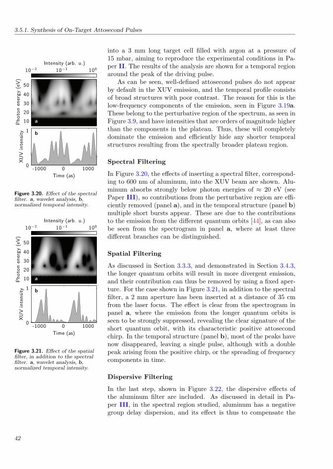
3.5.1. Synthesis of On-Target Attosecond Pulses
Time (as)
XU
Vin
tensity b
-1000 0 10000
1
Intensity (arb. u.)
10−2 10−1 100
Photo
nen
ergy
(eV)
a10
20
30
40
50
Figure 3.20. Effect of the spectralfilter. a, wavelet analysis, b,normalized temporal intensity.
Time (as)
XU
Vin
tensity b
-1000 0 10000
1
Intensity (arb. u.)
10−2 10−1 100
Photo
nen
ergy
(eV)
a10
20
30
40
50
Figure 3.21. Effect of the spatialfilter, in addition to the spectralfilter. a, wavelet analysis, b,normalized temporal intensity.
into a 3 mm long target cell filled with argon at a pressure of15 mbar, aiming to reproduce the experimental conditions in Pa-per II. The results of the analysis are shown for a temporal regionaround the peak of the driving pulse.
As can be seen, well-defined attosecond pulses do not appearby default in the XUV emission, and the temporal profile consistsof broad structures with poor contrast. The reason for this is thelow-frequency components of the emission, seen in Figure 3.19a.These belong to the perturbative region of the spectrum, as seen inFigure 3.9, and have intensities that are orders of magnitude higherthan the components in the plateau. Thus, these will completelydominate the emission and efficiently hide any shorter temporalstructures resulting from the spectrally broader plateau region.
Spectral Filtering
In Figure 3.20, the effects of inserting a spectral filter, correspond-ing to 600 nm of aluminum, into the XUV beam are shown. Alu-minum absorbs strongly below photon energies of ≈ 20 eV (seePaper III), so contributions from the perturbative region are effi-ciently removed (panel a), and in the temporal structure (panel b)multiple short bursts appear. These are due to the contributionsto the emission from the different quantum orbits [44], as can alsobe seen from the spectrogram in panel a, where at least threedifferent branches can be distinguished.
Spatial Filtering
As discussed in Section 3.3.3, and demonstrated in Section 3.4.3,the longer quantum orbits will result in more divergent emission,and their contribution can thus be removed by using a fixed aper-ture. For the case shown in Figure 3.21, in addition to the spectralfilter, a 2 mm aperture has been inserted at a distance of 35 cmfrom the laser focus. The effect is clear from the spectrogram inpanel a, where the emission from the longer quantum orbits isseen to be strongly suppressed, revealing the clear signature of theshort quantum orbit, with its characteristic positive attosecondchirp. In the temporal structure (panel b), most of the peaks havenow disappeared, leaving a single pulse, although with a doublepeak arising from the positive chirp, or the spreading of frequencycomponents in time.
Dispersive Filtering
In the last step, shown in Figure 3.22, the dispersive effects ofthe aluminum filter are included. As discussed in detail in Pa-per III, in the spectral region studied, aluminum has a negativegroup delay dispersion, and its effect is thus to compensate the
42
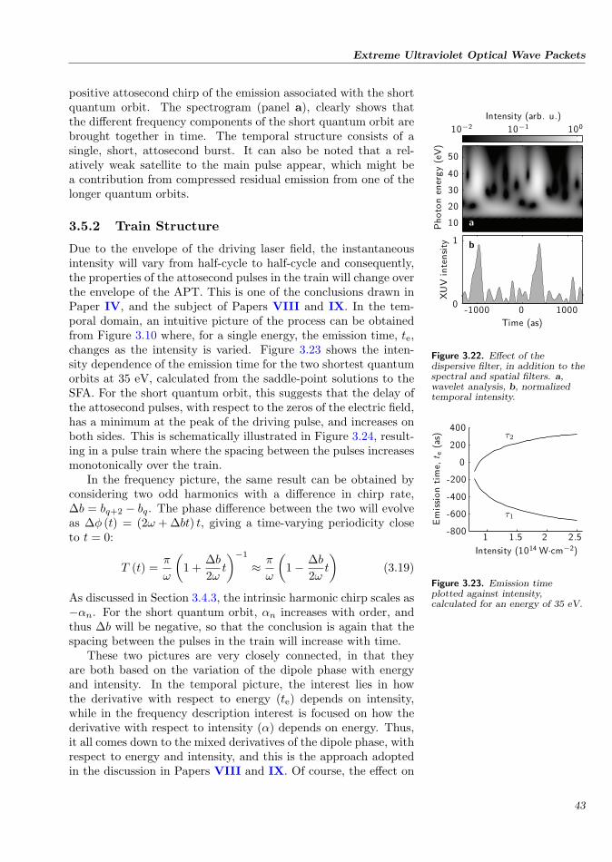
Extreme Ultraviolet Optical Wave Packets
Time (as)
XU
Vin
tensity b
-1000 0 10000
1
Intensity (arb. u.)
10−2 10−1 100
Photo
nen
ergy
(eV)
a10
20
30
40
50
Figure 3.22. Effect of thedispersive filter, in addition to thespectral and spatial filters. a,wavelet analysis, b, normalizedtemporal intensity.
Intensity (1014 W·cm−2)
Em
ission
tim
e,t e
(as)
τ1
τ2
1 1.5 2 2.5-800
-600
-400
-200
0
200
400
Figure 3.23. Emission timeplotted against intensity,calculated for an energy of 35 eV.
positive attosecond chirp of the emission associated with the shortquantum orbit. The spectrogram (panel a), clearly shows thatthe different frequency components of the short quantum orbit arebrought together in time. The temporal structure consists of asingle, short, attosecond burst. It can also be noted that a rel-atively weak satellite to the main pulse appear, which might bea contribution from compressed residual emission from one of thelonger quantum orbits.
3.5.2 Train Structure
Due to the envelope of the driving laser field, the instantaneousintensity will vary from half-cycle to half-cycle and consequently,the properties of the attosecond pulses in the train will change overthe envelope of the APT. This is one of the conclusions drawn inPaper IV, and the subject of Papers VIII and IX. In the tem-poral domain, an intuitive picture of the process can be obtainedfrom Figure 3.10 where, for a single energy, the emission time, te,changes as the intensity is varied. Figure 3.23 shows the inten-sity dependence of the emission time for the two shortest quantumorbits at 35 eV, calculated from the saddle-point solutions to theSFA. For the short quantum orbit, this suggests that the delay ofthe attosecond pulses, with respect to the zeros of the electric field,has a minimum at the peak of the driving pulse, and increases onboth sides. This is schematically illustrated in Figure 3.24, result-ing in a pulse train where the spacing between the pulses increasesmonotonically over the train.
In the frequency picture, the same result can be obtained byconsidering two odd harmonics with a difference in chirp rate,∆b = bq+2 − bq. The phase difference between the two will evolveas ∆φ (t) = (2ω + ∆bt) t, giving a time-varying periodicity closeto t = 0:
T (t) =π
ω
(1 +
∆b
2ωt
)−1
≈ π
ω
(1− ∆b
2ωt
)(3.19)
As discussed in Section 3.4.3, the intrinsic harmonic chirp scales as−αn. For the short quantum orbit, αn increases with order, andthus ∆b will be negative, so that the conclusion is again that thespacing between the pulses in the train will increase with time.
These two pictures are very closely connected, in that theyare both based on the variation of the dipole phase with energyand intensity. In the temporal picture, the interest lies in howthe derivative with respect to energy (te) depends on intensity,while in the frequency description interest is focused on how thederivative with respect to intensity (α) depends on energy. Thus,it all comes down to the mixed derivatives of the dipole phase, withrespect to energy and intensity, and this is the approach adoptedin the discussion in Papers VIII and IX. Of course, the effect on
43

3.5.3. APT CharacterizationIR
inte
nsity a
0
1
t e(a
s)
b
-800
-550
-300
XU
Vin
tensity c
0
1
Time (fs)
Per
iod,T
(as)
d
-15 0 15
1200
1350
1500
Figure 3.24. Illustration of thepulse-to-pulse variations withinthe APT, that appear due to theenvelope of the driving pulse. a,intensity of the driving pulse andb, the corresponding emissiontime calculated using the SFA foran energy of 22 eV. c, pulse trainconstructed from the calculatedemission times, with vertical linesindicating the equally spacedzeros of the driving field, and d,the periodicity obtained from thecalculated emission times.
the delay of the attosecond pulses described above is only the first-order effect, while in Paper IX higher-order effects are included,such as the variation of the chirp of the attosecond pulses over thetrain, as well as the variation of the CEP of the attosecond pulses.
In connection with this discussion, it is interesting to returnto the transfer of chirp from the fundamental to the harmonics,demonstrated by the experiments described in Paper IV, and dis-cussed in Section 3.4.3. As can be seen in Equation (3.18), afundamental chirp, b1, will lead to a chirp difference of 2b1 be-tween two consecutive harmonics. From Equation (3.19), it canbe seen that this will result in an additional linear variation ofthe periodicity of the pulses. The corresponding temporal descrip-tion is that when the fundamental pulse is chirped, the zeros ofthe field are redistributed in time in a linear fashion, and withthem the attosecond bursts. Thus, an interesting aspect of theexperiments on chirp transfer, is that they provide a possibility tocontrol the structure of the pulse train by varying the chirp of thedriving field. In particular, in Paper IV the possibility of reachinga situation where all harmonics have more or less the same chirprates is demonstrated, implying that the corresponding temporalstructure is a train of equally spaced pulses.
3.5.3 APT Characterization
For the characterization of pulses in an APT, a method known asreconstruction of attosecond beating by interference of two-photontransitions (RABITT) [92], has been used for the experiments pre-sented here. It is an indirect method, where the phase differences,∆φq+1, between consecutive harmonics are measured and used to-gether with the harmonic amplitudes to reconstruct the attosecondpulses [24]. The phase difference can be interpreted as a group de-lay (see Section 1.3.2), expressed as:
td =∂φ (Ω)
∂Ω≈ ∆φq+1
2ω=
φq+2 − φq
2ω(3.20)
where φq is the phase of harmonic q. This group delay representsthe delay of frequency components centered around Ω = (q + 1) ω.
Sideband Interference
As mentioned in Section 3.4.2, in a cross-correlation trace like theone shown in Figure 3.14, there will be two contributions to eachsideband: one from each of the neighboring harmonic peaks. If thecross-correlation setup allows for interferometric precision, throughthe stability of the pump-probe delay, but also in terms of thewavefront matching in the overlap region, it will be possible toobserve interference between these contributions [31]. In addition,
44

Extreme Ultraviolet Optical Wave Packets
Pulse fromthe laser
Pump pulse
Probe pulse
Beamsplitter
Harmonic generation
Aluminum filter
Recombination mirror
Toroidalmirror MBES
Variable delay
Figure 3.25. Mach-Zehnder type cross-correlation setup used for theRABITT measurements.
this interference will be modulated by the delay τ between theprobe field and the XUV field, with the modulated part given by:
Sq+1 (τ) ∝ cos (2ωτ −∆φq+1 −∆ϕat) (3.21)
where ∆φq+1 is the sought phase difference between the two har-monics involved, introduced above. The term ∆ϕat is a correctionterm due to the variation of the atomic dipole phase [31], discussedin Section 2.1.1 and Papers III and XI. The effect of this correc-tion on the resulting pulse length is usually very small, and canoften be neglected, especially at high energies.
Experimental Setup
The RABITT measurements require a stability in the pump-probedelay on the attosecond time-scale, translating into a few tens ofnanometers in the length of the arms of the interferometer. Thisis achieved by using a Mach-Zehnder configuration, shown in Fig-ure 3.25. The interferometer is built on a single optical table, andvibration dampers are used for all vacuum pumps. The laser pulseis split into a pump and a probe pulse, and the pump pulse is usedto generate the APT, while the probe pulse is routed through avariable delay line, controlled by a piezo-electric actuator. The re-maining IR pump light is blocked by an aluminum filter before theXUV pulses are recombined with the probe pulses. The geometryused for the recombination of the two beams is slightly differentfrom that used for the XFROG measurements (see Figure 3.15),using here a convex mirror with a hole at the center. The XUVpulses are sent through the hole from the back of the mirror, whilethe annular part of the probe beam is reflected off the mirror to
45
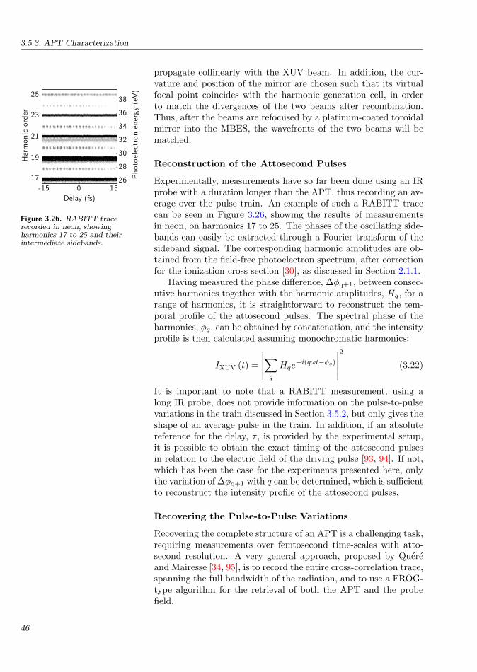
3.5.3. APT Characterization
Delay (fs)
Har
monic
ord
er
-15 0 15
17
19
21
23
25
Photo
elec
tron
ener
gy
(eV)
26
28
30
32
34
36
38
Figure 3.26. RABITT tracerecorded in neon, showingharmonics 17 to 25 and theirintermediate sidebands.
propagate collinearly with the XUV beam. In addition, the cur-vature and position of the mirror are chosen such that its virtualfocal point coincides with the harmonic generation cell, in orderto match the divergences of the two beams after recombination.Thus, after the beams are refocused by a platinum-coated toroidalmirror into the MBES, the wavefronts of the two beams will bematched.
Reconstruction of the Attosecond Pulses
Experimentally, measurements have so far been done using an IRprobe with a duration longer than the APT, thus recording an av-erage over the pulse train. An example of such a RABITT tracecan be seen in Figure 3.26, showing the results of measurementsin neon, on harmonics 17 to 25. The phases of the oscillating side-bands can easily be extracted through a Fourier transform of thesideband signal. The corresponding harmonic amplitudes are ob-tained from the field-free photoelectron spectrum, after correctionfor the ionization cross section [30], as discussed in Section 2.1.1.
Having measured the phase difference, ∆φq+1, between consec-utive harmonics together with the harmonic amplitudes, Hq, for arange of harmonics, it is straightforward to reconstruct the tem-poral profile of the attosecond pulses. The spectral phase of theharmonics, φq, can be obtained by concatenation, and the intensityprofile is then calculated assuming monochromatic harmonics:
IXUV (t) =
∣∣∣∣∣∑q
Hqe−i(qωt−φq)
∣∣∣∣∣2
(3.22)
It is important to note that a RABITT measurement, using along IR probe, does not provide information on the pulse-to-pulsevariations in the train discussed in Section 3.5.2, but only gives theshape of an average pulse in the train. In addition, if an absolutereference for the delay, τ , is provided by the experimental setup,it is possible to obtain the exact timing of the attosecond pulsesin relation to the electric field of the driving pulse [93, 94]. If not,which has been the case for the experiments presented here, onlythe variation of ∆φq+1 with q can be determined, which is sufficientto reconstruct the intensity profile of the attosecond pulses.
Recovering the Pulse-to-Pulse Variations
Recovering the complete structure of an APT is a challenging task,requiring measurements over femtosecond time-scales with atto-second resolution. A very general approach, proposed by Quereand Mairesse [34, 95], is to record the entire cross-correlation trace,spanning the full bandwidth of the radiation, and to use a FROG-type algorithm for the retrieval of both the APT and the probefield.
46

Extreme Ultraviolet Optical Wave Packets
Harmonicgeneration Aluminum
filter Aperture
Time (fs)
Inte
nsity
-1 0 1
Time (fs)
Inte
nsity
-1 0 1
Time (fs)
Inte
nsity
-1 0 1
Figure 3.27. Setup used for the post-compression experiments. Theamount of compensation can be controlled by varying the number ofaluminum filters. The insets show the results of TDSE calculations forthe temporal structure of the pulses at the different positions in thesetup.
In Paper VII, a different approach is proposed, which can bedescribed as a combination of the XFROG and RABITT tech-niques. In principle, by using an interferometrically stable setupin combination with a short probe pulse, the measurement of therelative harmonic phases will be done locally in the pulse train.By extracting the phase of the oscillation over the full sidebandtogether with the sideband tilt, the complete structure of the APTcan be recovered, assuming linearly chirped harmonics. In prac-tice, corrections have to be made to compensate for the duration ofthe probe pulse, as discussed in Paper VII, where the reconstruc-tion from a calculated cross-correlation trace is demonstrated.
A third, more indirect method, is presented in Paper IX, wherea Taylor expansion in time and energy is performed for the phaseof the total field. The idea is based on measuring the coefficients ofthe expansion, using RABITT measurements at different intensi-ties, combined with XFROG measurements for different harmonicorders. Knowing the coefficients, it is possible to carry out anadiabatic reconstruction of the APT.
3.5.4 Attosecond Pulse Generation andCompression
Several routes have been suggested to compensate for the intrin-sic attosecond chirp, using, for example, XUV chirped multi-layermirrors [96], the negative electron dispersion in a plasma [46] ormetallic filters with negative group velocity dispersion [46, 97].
In Paper II, the latter method was implemented, using filtersmade of aluminum, whose properties are detailed in Paper III.The APT was generated from argon, and in the preparation of theattosecond pulses, depicted in Figure 3.27, the recipe given in Sec-
47

3.5.5. Trains with One Pulse per Laser Cycle
Group delay, td (as)
Photo
nen
ergy,
hΩ
(eV)
b
-400 0 40020
30
40
50
Time (as)
Inte
nsity
(arb
.u.)
a
-400 0 4000
1
Figure 3.28. Post-compression ofattosecond pulses using aluminumfilters. a, reconstructed temporalprofiles using 200 nm (dashedline) and 600 nm (solid line) ofaluminum. b, the correspondinggroup delays for 200 nm (circles)and 600 nm (squares) ofaluminum.
tion 3.5.1 was followed, using the transmission of the aluminumfilter for the spectral selection, an aperture to remove contribu-tions from all but the short quantum orbit, and the dispersionof the filter to compensate for the intrinsic positive chirp of theattosecond pulses. Figure 3.28a shows the reconstructed temporalprofiles of the pulses after propagation through 200 nm (dashedline) and 600 nm (solid line) of aluminum. Panel b shows thecorresponding measured group delays, td, for 200 nm (circles) and600 nm (squares) of aluminum. Varying the filter thickness, it waspossible to control the amount of compensation, and by increasingthe thickness from 200 nm to 600 nm, the pulses were compressedfrom 280 as down to 170 as, where the latter corresponds to only1.2 electric field cycles at the central photon energy (30 eV).
3.5.5 Trains with One Pulse per Laser Cycle
So far, only the generation of attosecond pulse trains using amonochromatic driving field has been considered, which, due tothe half-cycle anti-symmetry of the field in combination with thesymmetry of the medium, results in pulses with identical envelopes,separated by half an IR cycle, with a phase shift of π betweenconsecutive pulses. In Section 3.4.1, it was discussed that it isexactly this phase shift, in combination with the repetition rate,that causes only the odd harmonics to appear in the spectrum.
For some experiments, such as those presented in Papers XIIIand XIV and discussed in Section 4.3, it is useful to have atrain with two pulses per laser cycle, since, in the presence ofa strong laser field, each ejected EWP will experience an oppo-site shift in momentum relative to the previous one, as discussedin Section 4.1.3. However, for many experiments, this is an am-biguity that leads to difficulties in the interpretation of the ex-perimental results. In addition, removing alternate pulses fromthe train, will mean that all pulses are generated under identicalconditions, and thus will have the same CEP. Knowing that itis possible to produce attosecond pulses with durations close tothe single-cycle limit, by using external phase compensation, asdemonstrated in Paper II, this is indeed an interesting approachto extending the concept of few-cycle, phase-stabilized pulses intothe XUV regime [91, 98–100].
In the experiment described in Paper VI, the production of anAPT with a repetition period of one IR laser cycle was demon-strated. By including the second harmonic of the IR field in theXUV generation, the half-cycle-to-half-cycle anti-symmetry wasbroken and, for a wide range of delays between the IR field and itssecond harmonic, it was shown experimentally that the emissionwas dominated by a single attosecond pulse per IR cycle. Below,the interferometer used to create the two-color driving field is de-
48

Extreme Ultraviolet Optical Wave Packets
Laserpulse
KDPtype I
ω,↔
ω,↔2ω,
ω,↔2ω,
λ/2
2ω,↔
Pump pulse
ω,↔2ω,↔
ω,↔
Probe pulse
Delay plateVariable delay
DBS
BS
DBS
Figure 3.29. Two-color Michelson interferometer used to create thepump pulses for the generation of APTs with one pulse per laser cy-cle. At different points in the interferometer, the labels indicate thefrequency (ω or 2ω) of the pulses, and their polarization (↔, horizontalor l, vertical). BS, beam splitter; DBS, dichroic beam splitter; λ/2,half-wave plate.
scribed, and the spectral measurements are discussed together withresults and predictions of the SFA and the semi-classical model.
Two-Color Interferometer
To create the two-color driving field a two-color Michelson inter-ferometer, shown in Figure 3.29, was used. The incoming, horizon-tally polarized, laser pulse is frequency doubled in a type I KDP11
crystal, so that the second harmonic pulse is created with verticalpolarization. Using a dichroic beam splitter, the second harmonicpulse is separated from the IR pulse and routed through a variabledelay line, before a half-wave plate is used to rotate its polarizationback to horizontal, matching its polarization with that of the IRpulse. The variable delay is introduced using mirrors mounted on atranslation stage, and is only used to find the overlap between thetwo pulses, while in the other arm of the interferometer, a rotat-able 100 µm thick delay plate is used to obtain a fine adjustmentof the relative arm lengths. Before the two pulses are recombined,by means of a dichroic beam splitter, part of the IR pulse is splitoff using another beam splitter, to be used as a probe for the mea-surements. In the pump-probe experiment presented in Paper VI,the two-color Michelson interferometer simply replaced the beamsplitter in Figure 3.25.
11potassium dihydrogen phosphate
49

3.5.5. Trains with One Pulse per Laser Cycle
Photon energy (eV)
Inte
nsity
(arb
.u.
)
a
20 30 400
0.5
1
Photon energy (eV)
e
20 30 40
Photon energy (eV)
Inte
nsity
(arb
.u.
)
b0 20 40 60 8010−10
100
Photon energy (eV)
f0 20 40 60 80
Time (as)
Inte
nsity
(arb
.u.
)
c
-2000 0 2000-1
0
1
Time (as)
g
-2000 0 2000
Time (as)
Ret
urn
ener
gy(U
P)
d
-2000 0 20000
2
4
Time (as)
h
-2000 0 2000
Figure 3.30. Experimental results and theoretical predictions for thegeneration of an APT using a two-color field. a-d correspond to thedelays for which the harmonic yield is minimum, while e-h correspondto the maximum harmonic yield (see text). a and b show experimentalspectra, using only the IR field (gray shaded areas), and both the IR fieldand its second harmonic (black lines). b and f, spectra calculated usingthe SFA. The total spectra are shown by the thick gray lines, while theblack lines show the separate contributions from electrons ionized whenthe field is either positive or negative. c and g, shape of the electric field(gray lines) together with the temporal structure calculated using theSFA. d and h, classical return energy, represented in grayscale accordingto the strength of the electric field at the time of ionization (from whiteto black for increasing field strengths).
50

Extreme Ultraviolet Optical Wave Packets
Spectral and SFA Results
The result of adding the second harmonic to the generation is theappearance of both odd and even harmonics of the IR field [101–103], due to the change in periodicity of the generation process.As shown in Figure 2 of Paper VI, experimentally a modulationof the total harmonic yield is found as the delay between the IRpulse and its second harmonic is changed. Figure 3.30 focuseson the two delays for which the yield is minimum (panels a-d)and maximum (panels e-h). Panels a and b show experimentallymeasured spectra, using only the IR field (gray shaded areas), andboth the IR field and its second harmonic (black lines).
When the minimum yield is obtained, the harmonic peakstrengths vary considerably from peak to peak (panel a), whilefor the maximum yield, the harmonic peaks follow a smooth spec-tral envelope (panel b). The same delay dependence is found inthe spectra calculated using the SFA, shown by the gray lines inpanels b and f. Panels c and g show the shape of the electric fieldfor the two delays, together with the temporal structure of theemission, calculated using the SFA. As can be seen, for the delaycorresponding to minimum harmonic yield, there are two pulses ofcomparable intensity per IR cycle, one of them resulting from elec-trons ionized when the electric field is negative, and one when thefield is positive. In the SFA, these two contributions can be sepa-rated, and each of them is shown (black lines) in panel b. In thiscase, the spectra from the two contributions are very similar, andthe irregular behavior observed in the total spectrum is a result ofinterference between the two. In the case of maximum harmonicyield (panel g), there is only one pulse per IR cycle and, as canbe seen in panel f, this is the result of one of the contributionsdominating in the spectrum.
Finally, in panels d and h, the classical return times are shown,calculated for the two-color field, where the lines are representedin grayscale according to the strength of the electric field at thetime the electron was ionized (increasing from white to black).The semi-classical model gives an intuitive picture of the processin the case of a single pulse per cycle (panel h). In this case,one of the re-collisions contain electrons ionized by a weak electricfield (low ionization probability), and returning with a high energy(high cut-off energy), while the other re-collision contains electronsionized with a high probability, but with low cut-off energies, likethe two contributions to the spectrum shown in panel f.
Paper VI, presents temporal measurements experimentallyconfirming the predicted time structures for different delays. Theseare also discussed in Section 4.1.3.
51

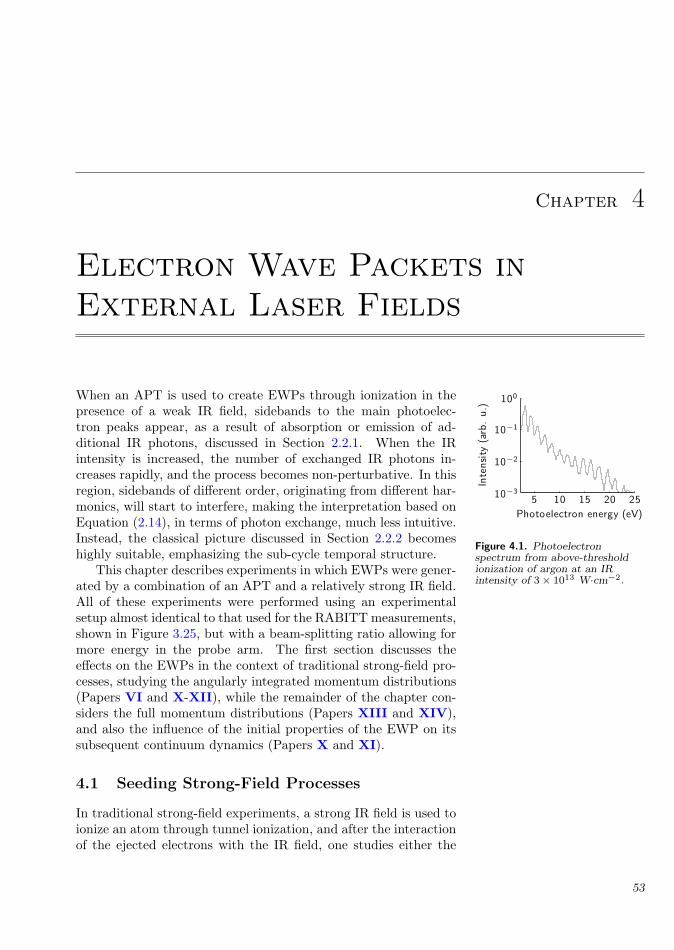
Photoelectron energy (eV)
Inte
nsity
(arb
.u.)
5 10 15 20 2510−3
10−2
10−1
100
Figure 4.1. Photoelectronspectrum from above-thresholdionization of argon at an IRintensity of 3× 10¹³ W·cm−2.
Chapter 4
Electron Wave Packets inExternal Laser Fields
When an APT is used to create EWPs through ionization in thepresence of a weak IR field, sidebands to the main photoelec-tron peaks appear, as a result of absorption or emission of ad-ditional IR photons, discussed in Section 2.2.1. When the IRintensity is increased, the number of exchanged IR photons in-creases rapidly, and the process becomes non-perturbative. In thisregion, sidebands of different order, originating from different har-monics, will start to interfere, making the interpretation based onEquation (2.14), in terms of photon exchange, much less intuitive.Instead, the classical picture discussed in Section 2.2.2 becomeshighly suitable, emphasizing the sub-cycle temporal structure.
This chapter describes experiments in which EWPs were gener-ated by a combination of an APT and a relatively strong IR field.All of these experiments were performed using an experimentalsetup almost identical to that used for the RABITT measurements,shown in Figure 3.25, but with a beam-splitting ratio allowing formore energy in the probe arm. The first section discusses theeffects on the EWPs in the context of traditional strong-field pro-cesses, studying the angularly integrated momentum distributions(Papers VI and X-XII), while the remainder of the chapter con-siders the full momentum distributions (Papers XIII and XIV),and also the influence of the initial properties of the EWP on itssubsequent continuum dynamics (Papers X and XI).
4.1 Seeding Strong-Field Processes
In traditional strong-field experiments, a strong IR field is used toionize an atom through tunnel ionization, and after the interactionof the ejected electrons with the IR field, one studies either the
53

4.1.1. Below-Threshold Injection
Inte
nsity
a Xe
0
1
Photon energy (eV)
0 10 20 30 40 50
Harmonic order
Inte
nsity
b Ar
1 7 13 19 25 31 370
1Ar+ He+
Figure 4.2. Spectra of APTsgenerated in xenon (a) and argon(b), shown in relation to theionization potentials of argon andhelium.
Delay (as)
Ion
yiel
d(a
rb.
u.)
He+
Ar+
-1000 0 1000 20000
1
2
3
4
5
Figure 4.3. Experimental ionyields as a function of the delaybetween the APT and the IRfield. The ion yields arenormalized to the yields obtainedwith only the APT. The insetsshow the shape of the atomicpotential at the time of injectionby the attosecond pulses.
photons emitted when the electrons recombine, as discussed inChapter 3, or the electrons ejected [6, 7, 104]. Figure 4.1 showsa photoelectron spectrum from argon ionized by an IR field withan intensity of 3 × 10¹³ W·cm−2. The spectrum exhibits peaksspaced by the IR photon energy, due to the periodicity of theprocess which is equal to the laser period, reaching high energiesas a result of the electrons being accelerated by the IR field and re-scattered from the ion core [105, 106]. In this process, called above-threshold ionization, for a given atomic species all parameters aredetermined solely by the IR field, dictating when tunneling takesplace, what the initial properties of the EWP are, and finally whatits subsequent evolution will be.
In Papers X-XII, an APT was used to initiate the ionizationprocess, resulting in control of either the ionization yield (Pa-per XII), or the initial conditions for the evolution of the EWP inthe IR field (Papers X and XI). Finally, in Paper VI, the effect ofthe field on the injected EWP was used to confirm the predictedtemporal structure of an APT with a single pulse per IR cycle,previously discussed in Section 3.5.5.
4.1.1 Below-Threshold Injection
Figure 4.2a shows the spectrum of an APT generated in xenonused for the experiment presented in Paper XII. The pulses inthe APT have a central energy of ≈ 23 eV, and a pulse durationof 370 as, measured using the RABITT technique. The interestin these pulses lies in the fact that the photon energy is lowerthan the ionization potential of helium (24.6 eV), as indicated inFigure 4.2a, making single-photon ionization of helium possibleonly for the high-energy flank of the bandwidth, consisting of har-monic 17. In the experiment the velocity map imaging spectrom-eter (VMIS) was operated in ion TOF mode (see Section 2.3.3),and the yield of singly charged helium was studied as a functionof the delay between the APT and an IR field. Some of the resultsare presented in Figure 4.3, where it can be seen that as the IRfield is introduced, the He+ yield is enhanced by a factor of ≈ 4for all delays1. In addition, the yield is modulated with a depth ofmodulation of ≈ 35%, with maxima twice per laser cycle, close towhen the attosecond pulses overlap the peaks of the electric field.A suggested interpretation is that ionization takes place throughan “over-the-barrier” mechanism, where the EWP is most likely toescape when the Coulomb barrier is maximally suppressed by theelectric field of the laser [107], as shown by the insets in Figure 4.3.Thus, by using an APT with a central energy below the ionizationthreshold, in Paper XII the possibility of controlling the ioniza-
1For these measurements, the intensity of the IR field was 1.3 ×10¹³ W·cm−2, causing no measurable ionization by the IR field alone.
54

Electron Wave Packets in External Laser Fields
Inte
nsity
a10−2
10−1
100
Energy
Inte
nsity Xe/He
Inte
nsity
b10−2
10−1
100
Energy
Inte
nsity Xe/Ar
Photoelectron energy (eV)
Inte
nsity
c
0 10 20 30 4010−2
10−1
100
Energy
Inte
nsity Ar/Ar
Figure 4.4. Comparison of thephotoelectron spectra obtainedfrom ionization by an APT and arelatively strong IR field, fordifferent experimental conditions.The thin and the thick linescorrespond to different delaysbetween the two fields (see text).a, APT generated in xenon,detection in helium. b, generationin xenon, detection in argon. c,generation in argon, detection inargon. For a and b the IRintensity was 1.3× 10¹³ W·cm−2,and for c it was 3× 10¹³ W·cm−2.The insets show the spectra fromthe APT alone.
tion, by changing the delay between the attosecond pulses and theIR field, was shown.
The photoelectron momentum distributions were also studied(see Figure 4 of Paper XII), and, as expected, peaks spaced bythe IR photon energy, with intensities and cut-off energies stronglyvarying with the delay were found. The angular distributions werefound to be strongly peaked along the polarization direction ofthe IR field, very similar to the angular distributions found intraditional multi-photon ionization. Figure 4.4a shows the photo-electron spectra corresponding to the delay for which the highestenergy electrons are obtained (thin line) and a delay one quarterof a cycle away (thick line). Interestingly, it was found from the-oretical calculations that these delays do not exactly correspondto the delays for which the maximum and minimum ion yields areobtained, an observation which is further discussed in Paper XII.
4.1.2 Above-Threshold Injection
Argon has an ionization threshold of 15.8 eV, meaning that theentire bandwidth of the APTs used above will contribute to theproduction of Ar+ already in the field-free case, as shown in Fig-ure 4.2a. As a consequence of this, adding the IR field to theionization has no effect on the ion yield, as shown in Figure 4.3.In the photoelectron spectrum, however, dramatic effects appear,as shown in Figure 4.4b. For the delays when the attosecondpulses overlap the peaks of the laser field, sidebands appear andthe distribution is slightly broadened (thick line). When the pulsesoverlap the zero-crossings of the electric field, the distribution isstrongly broadened, with electrons appearing on both the low- andthe high-energy sides of the initial distribution (thin line). Con-sidering the full delay dependence of the photoelectron spectrum,shown in Figure 3 of Paper XII, it is clear that the effect of theIR field is merely to redistribute the electrons that are already inthe continuum after the single-photon step, an observation that isconsistent with the lack of modulation of the ion yield. This ef-fect is nothing but the momentum shift, discussed in Section 2.2.2,equal to the vector potential and is thus maximum or minimum atthe zero-crossings of the electric field.
The first experiments showing the resulting energy shift usingan APT are presented in Papers X and XI. An APT generated inargon was used, as shown in Figure 4.2b, having a higher centralenergy (≈ 30 eV) than the APT generated in xenon. The corre-sponding results are presented in Figure 4.4c, showing even moreclearly how the photoelectrons are redistributed to higher energieswhen overlapping the zeros of the laser field (thin line). In thiscase, the redistribution towards lower energies does not appearthat clearly, being partly hidden by low-energy electrons from ion-
55

4.1.3. Probing the Train Structure
a5
15
25
b5
15
25
Photo
elec
tron
ener
gy
(eV)
c5
15
25
Delay (fs)
d-4 -2 0 2 4
5
15
25
Figure 4.5. Photoelectron spectrafrom argon as a function of delayfor different APTs. a, APTgenerated by only the IR field.b-d, APTs generated using an IRfield plus its second harmonic forthree different delays between thetwo fields. To emphasize thehigh-energy behavior, eachphotoelectron peak is representedby a sum over the peak, and thesignal for each peak has beennormalized.
ization by the IR field alone2. For the full delay dependence of thephotoelectron spectrum, see Figure 2 of Paper X.
As discussed here, the experiments presented in Papers X-XIIshow that using APTs for the precise injection of EWPs into astrong IR field provides a way of controlling the subsequent elec-tron dynamics, with significant effects on the resulting photoelec-tron distributions. In Papers X and XI, it is shown how the initialtime-frequency properties of the EWPs can be influenced by theattosecond pulses, and how this affects the photoelectron distribu-tions (see also Section 4.2.2).
4.1.3 Probing the Train Structure
The reason why there is a shift towards both higher and lower en-ergies in the spectra of Figure 4.4b and c, is that an APT with twopulses per laser cycle was used. Thus, for each time, t, such thata certain EWP experiences a momentum shift −eA (t) [see Equa-tion (2.17)], the next EWP in the train will instead experience ashift −eA (t + π/ω) = eA (t). As a consequence, the photoelec-tron spectrum will vary with the delay between the APT and theIR field, with a period of half the laser cycle, as demonstrated inPapers X and XI.
In Paper VI, this effect was used to probe the periodicity ofthe APT generated using a two-color field. Figure 3 of Paper VIshows the delay dependence of the photoelectron spectrum for thecase of a clean APT with a single pulse per IR cycle, togetherwith the integrated high-energy signal for a few different cases. InFigure 4.5, the full delay-dependence of the photoelectron spec-tra corresponding to all those cases is shown. To emphasize thehigh-energy behavior, the spectra have been integrated over eachphotoelectron peak, and the resulting signal normalized with re-spect to the delay for each peak. Panel a shows the case when theAPT is generated by the IR field alone. As can be seen, the peri-odicity of the signal is half a laser cycle, 1.33 fs, indicating that,as expected, there are two, equally spaced, attosecond pulses percycle. In panels b-d, harmonics are created by mixing the funda-mental and its second harmonic. The spectra in panels b and d arerecorded for delays between the IR field and its second harmonicchosen so that the harmonic yield is maximized (corresponding toFigure 3.30e-h). The prediction of the SFA calculation is that forthese delays, a single attosecond pulse per IR cycle should domi-nate the emission, and indeed, this is confirmed by the repetitionrate, being equal to a full laser cycle, or 2.66 fs. Finally, panel cshows a result when the delay between the two fields is such thatthe harmonic yield is minimized. As predicted by the SFA (see
2For this measurement, the IR intensity was slightly higher (3 ×10¹³ W·cm−2), and thus, at low energies, photoelectrons from ionization bythe IR field alone can be observed.
56

Electron Wave Packets in External Laser Fields
Figure 3.30a-d), a satellite burst appears in the train, manifestingitself in the delay-dependent spectra as an additional high-energycontribution, appearing almost, but not exactly, in between thecontributions from the main pulse.
Thus, by letting the second harmonic of the driving field par-ticipate in the generation of the APT, in Paper VI it was shownthat for certain delays between the two fields, APTs with a singlepulse per IR cycle are generated. As will be shown in the nextsection, these pulse trains have the potential to be extremely use-ful, in that they remove the ambiguity resulting from having twopulses, and thus two different events, per cycle.
4.2 Three-Dimensional Wave Packet Dynamics
In the previous section, experiments were presented in which theinfluence of an IR laser field on an EWP was observed and eval-uated mainly from the photoelectron spectra. A great deal ofimportant information can be obtained from such measurements,but from Section 2.2.2, and in particular Figure 2.8, it is clearthat, in order to demonstrate the classical interpretation of theelectron dynamics, angularly resolved measurements are needed.This section will discuss how the momentum shift of an EWP ina laser field will manifest itself when instead of a single EWP, atrain of EWPs is used, and this will be illustrated by showing somerecent experimental results. It will also be shown how the initialproperties of the EWP can change its dynamics in the field, aneffect observed in the experiments presented in Papers X and XI.
4.2.1 Control of the Final Momentum
As shown in Figure 2.8, the momentum distribution of an EWPgenerated from ionization by a single XUV pulse significantlyshorter than the period of the IR field will experience a shift inmomentum equal to −eA (t), through its interaction with the laserfield. If instead a pulse train with a single pulse per IR cycle, asdiscussed above, is used for ionization, each EWP in the train willexperience the same momentum shift, as illustrated in Figure 4.6a-e, leading to an effect very similar to the one observed for singleEWPs. What differs between the two results is that interferencerings appear when a pulse train is used, centered at the origin,arising from the repetition of the ionization process. The max-ima of these rings will, as discussed in Section 3.5.5, correspondto harmonics (odd and even) of the IR frequency, shifted by theionization potential of the atom plus the ponderomotive shift.
In a recent experiment [108], an APT with one pulse per cyclewas generated from argon, using the two-color technique presentedin Paper VI and Section 3.5.5. This train was used to create EWPs
57

4.2.1. Control of the Final Momentum
p y(1
0−24
Ns) a
-2 0 2
-2
0
2 b
-2 0 2
px (10−24 Ns)
c
-2 0 2
d
-2 0 2
e
-2 0 2
p y(1
0−24
Ns)
f
-2 0 2
-2
0
2 g
-2 0 2
px (10−24 Ns)
h
-2 0 2
i
-2 0 2
j
-2 0 2
Figure 4.6. Calculated electron momentum distributions from heliumionized by XUV pulses with a duration of 300 as and a central energy of39 eV, in the presence of an IR field with an intensity of 1×10¹³ W·cm−2.The pulses are delivered in an APT with one pulse per IR cycle (a-e)and two pulses per IR cycle (f-j). Above the momentum maps the delaybetween the XUV pulses (black line) and the vector potential of the IRfield (gray line) is indicated.
by ionization of argon, and the possibility of controlling the finalmomentum of these wave packets was demonstrated, through an-gularly resolved measurements of the photoelectron distributions.The first results are shown in Figure 4.7a-e. Without an IR field(panel a), one can clearly see the peaks corresponding to odd andeven harmonics. When ionization takes place at the zero-crossingsof the vector potential (panels b and d), broadening of the momen-tum distributions is seen in the direction of the laser polarization,an effect of the duration of the EWP, as different temporal parts ofthe EWP experience different momentum shifts (see Section 2.2.2).When ionization takes place at the peaks of the vector potential,steering of the electrons can clearly be seen, either along the pos-itive (panel c) or the negative (panel e) py-axis.
From these first measurements, it can be concluded that theambiguity of having two different events per cycle is removed whenusing an APT with a single pulse per IR cycle. Thus, these APTsprovide a tool useful for performing control experiments, previ-ously exclusively reserved to isolated attosecond pulses. In addi-tion, being synthesized from the emission plateau rather than thecut-off, APTs give access to large bandwidths and higher intensi-ties, with the possibility of injecting low-energy EWPs. An inter-
58

Electron Wave Packets in External Laser Fields
p y(1
0−24
Ns) a
-2 0 2
-2
0
2 b
-2 0 2
px (10−24 Ns)
c
-2 0 2
d
-2 0 2
e
-2 0 2
p y(1
0−24
Ns) f
-2 0 2-2
0
2 g
-2 0 2
px (10−24 Ns)
h
-2 0 2
i
-2 0 2
j
-2 0 2
Figure 4.7. Experimental momentum distributions from ionization ofargon by XUV pulses in the presence of an IR field. a-e, using an APTwith one pulse per cycle, generated by a two-color field from argon.The central energy of the pulses was ≈ 24 eV, and the pulse durationwas estimated to 300 as. a-e using an APT with two pulses per cyclegenerated in xenon. The central energy was ≈ 23 eV, and the pulseduration 370 as. Above the momentum maps the delay between theXUV pulses (black line) and the vector potential of the IR field (grayline) is indicated.
esting effect of the latter statement is demonstrated in Figure 4.7cand e, where it can be seen that for the delays corresponding tothe maximum momentum shifts, some electrons are even “turnedaround”, having their direction along the py-axis changed throughthe interaction with the IR field.
In the experiments presented in Papers XII-XIV, the momen-tum distributions from APTs with two pulses per IR cycle werestudied. As already mentioned in Section 4.1.3, when these areoverlapped by an IR field, each EWP will be shifted in momentumin the opposite direction to the previous one. This is illustratedin Figure 4.6f -j, showing the results of calculations in helium. Forthe APT alone (panel f), interference rings are seen, correspond-ing to ionization by odd harmonics of the IR frequency. As can beseen, when overlapping the zero-crossings of the vector potential(panels g and i), the same broadening as before appears, whileoverlapping with the maxima and minima (panels h and j) of thevector potential shifts consecutive EWPs in opposite directions,giving rise to two clearly distinguishable rings in the momentumdistributions. For both delays, it can be seen that an additionalinterference structure, apart from the one arising from the peri-
59

4.2.2. Chirped Electron Wave Packets
p y(1
0−24
Ns) a
-2 0 2
-2
0
2 b
-2 0 2
px (10−24 Ns)
c
-2 0 2
d
-2 0 2
e
-2 0 2
Figure 4.8. Electron momentum distributions from helium ionized byan XUV pulse with a central energy of 39 eV, in the presence of an IRfield. The XUV pulse has a positive chirp, leading to a pulse durationof 350 as compared to its transform-limited duration of 300 as. The IRintensity used was 1 × 10¹³ W·cm−2. Above the momentum maps thedelay between the XUV pulses (black line) and the vector potential ofthe IR field (gray line) is indicated.
odicity of the process, appears where the momentum distributionsoverlap. These structures are the subject of Papers XIII and XIV,and are further discussed in Section 4.3. In Figure 4.7f -j, resultsfrom Paper XII are shown, where an APT generated in xenonis used to ionize argon in the presence of an IR field with an in-tensity of 1.3 × 10¹³ W·cm−2. These results agree well with theeffects predicted by the calculation, although it is not possible toobserve any separation of the two rings, due to the initially broadmomentum distribution.
4.2.2 Chirped Electron Wave Packets
The dynamics of an EWP injected into an IR field will depend, notonly on its energy, the time of injection and the strength of the IRfield, but also on the time-frequency properties of the unperturbedEWP3. This dependence is studied in the experiments presentedin Papers X and XI, where dispersive filtering of the pulses in theAPT, using aluminum filters (see Paper II), is used as a way toalter the attosecond chirp rate of the XUV pulses, and thus of theinjected EWPs.
As already discussed above, due to the durations of the EWPs,different temporal slices will appear in the continuum at differentvalues of the vector potential, and thus experience different mo-mentum shifts. In the case of transform-limited EWPs, discussedso far, this results in broadening along the polarization directionof the IR field, seen for example in Figure 2.8. In the case ofchirped EWPs, the situation becomes somewhat more complex,as shown in Figure 4.8. A clear asymmetry appears when ioniza-
3The properties of the unperturbed EWP denotes the initial properties ofthe EWP, when injected into the continuum without an IR field.
60

Electron Wave Packets in External Laser Fields
tion takes place at the zero-crossings of the vector potential; onepart of the EWP becomes broadened, while the other part is nar-rowed. This can be explained through realizing that a chirp in theenergy of the EWP, also means that it is chirped in momentum.When overlapping with the zero-crossings of the vector potential,the momentum shift due to the field varies in time over the EWP,imposing an additional chirp on the EWP along the py-axis. Onone side of the plane py = 0, the chirp imposed by the IR field willadd to the chirp of the unperturbed EWP, thus broadening its mo-mentum distribution, while on the other side, it will compensatethe chirp, narrowing the distribution.
The effect of the varying momentum shift is in principle that ofa streak camera, and as suggested in [109, 110] and implementedin [111], by studying the energy distribution of electrons alonga well-defined direction, this effect can be used to measure thelinear chirp of isolated attosecond XUV pulses. In the experimentspresented in Papers X and XI, these effects were observed in theangularly integrated photoelectron spectra, and in addition it wasshown that by using dispersive filtering to shape the attosecondXUV pulses, the properties of the injected EWPs could be altered,and the result observed in the continuum dynamics (see Figures 2and 3 in Paper X).
4.3 Electron Wave Packet Interferometry
At the points in momentum space where two or more EWPs over-lap, an interference structure will appear, in addition to the inter-ference that is seen as a result of the repetition. In the experimentspresented in Papers XIII and XIV, different aspects of these in-terference patterns were studied, using APTs with two pulses perIR cycle. Below, the results from these papers are briefly reviewed,starting with a more general model of the interference.
4.3.1 Interference between Electron Wave Packets
An EWP is described by its momentum distribution:
a (p) = Ae (p) eiφe(p) (4.1)
where Ae (p) and φe (p) are the amplitude and phase of the wavepacket. If this EWP is exposed to an IR field at a time ti, assumingthat its duration is very short compared to the period of the field(see Section 2.2.2), its final amplitude distribution can be writtenas:
a (p, ti) = Ae [p + eA (ti)] eiφe[p+eA(ti)]+φIR(p,ti)
= Ae (pi) ei[φe(pi)+φIR(p,ti)] (4.2)
61

4.3.1. Interference between Electron Wave Packets
where pi = p + eA (ti), A (t) is the vector potential of the IRfield, and φIR is the phase modulation of the EWP caused by theIR field, as defined in Equation (2.7). If two identical EWPs areinjected into the IR field at times t1 and t2, their contributionshave to be added coherently, resulting in a electron probabilitydistribution given by:
P (p, t1, t2) =∣∣∣∣a (p, t1) ei p2
2mh t1 + a (p, t2) ei p2
2mh t2
∣∣∣∣2= |Ae (p1)|2 + |Ae (p2)|2
+ 2Ae (p1) Ae (p2) cos
p2
2mh(t2 − t1)
+ φe (p2)− φe (p1) + φIR (p, t2)− φIR (p, t1)
= Λ (p1,p2)
1 + Γ (p1,p2) cos[
p2
2mh(t2 − t1)
+ ∆φe (p1,p2) + ∆φIR (p, t1, t2)]
(4.3)
with:
Λ (p1,p2) = |Ae (p1)|2 + |Ae (p2)|2
Γ (p1,p2) =2Ae (p1) Ae (p2)
Λ (p1,p2)∆φe (p1,p2) = φe (p2)− φe (p1)
∆φIR (p, t1, t2) = φIR (p, t2)− φIR (p, t1) (4.4)
As can be seen from the last step of Equation (4.3), the resultinginterference pattern will, to a first approximation, consist of circu-lar fringes arising from the term p2 (t2 − t1) /2mh. This is simplythe interference arising from the repetition, with a fringe spacingthat depends on the delay between the two EWPs, and the tworemaining terms in the cosine will lead to a shift of these fringes.The first term, ∆φe (p1,p2), is the phase difference between thetwo momentum components p1 and p2, which are brought togetherto interfere, while the second term, ∆φIR (p, t1, t2), is the phaseacquired in the IR field by the first EWP between the times t1 andt2. Assuming a linearly polarized IR field, E (t) = eE0 sin (ωt),Equations (2.8), (2.9) and (2.10) may be used to write the phasedifference induced by the IR field as:
∆φIR (p, t1, t2) =UP
h(t2 − t1) +
12hω
×
4
√UP
mp · e [sin (ωt2)− sin (ωt1)]
+ UP [sin (2ωt2)− sin (2ωt1)]
(4.5)
62

Electron Wave Packets in External Laser Fields
p y(1
0−24
Ns) a
-2 0 2
-2
0
2 b
-2 0 2
px (10−24 Ns)
c
-2 0 2
d
-2 0 2
e
-2 0 2
Figure 4.9. Calculated electron momentum distributions from heliumionized by two attosecond pulses, separated by half an IR cycle, in thepresence of an IR field. The XUV pulses have a central energy of 39 eV,durations of 300 as and the IR intensity was 1× 10¹³ W·cm−2. Abovethe momentum maps the delay between the XUV pulses (black line)and the vector potential of the IR field (gray line) is indicated.
where UP = e2E20
4mω2 is the ponderomotive energy. The first termhere causes an inward shift, i.e. a decrease in the radius, of thecircular fringes, by a distance corresponding to a kinetic energy ofUP. Thus, this is nothing but the ponderomotive shift, previouslydiscussed in Section 2.2.1. The last term also corresponds to achange in radius of the fringes, but now with a magnitude thatchanges with t1 and t2, while the remaining term causes morecomplex fringe shifts, as discussed below.
Two Electron Wave Packets per Cycle
In the following, EWPs separated by exactly half an IR cycle willbe considered. In this case, the delay between two consecutiveEWPs is always t2− t1 = π/ω, so Equation (4.5) can be simplifiedto:
∆φIR (p, t1) =π
hω
[UP −
4π
√UP
mp · e sin (ωt1)
](4.6)
Assuming that ∆φe (p1,p2) is constant, it is possible to show fromEquation (4.3) that the center of the interference circles, pc, willdepend on the timing with respect to the IR field as:
pc (t1) =4√
mUP
πsin (ωt1) e
=2e
πωE (t1) (4.7)
Thus, the interference fringes will be shifted off-center out of phasewith the shift of the overall momentum distributions, whose shiftis proportional to the vector potential. This effect is illustrated bythe calculated momentum distributions in Figure 4.9, where two
63
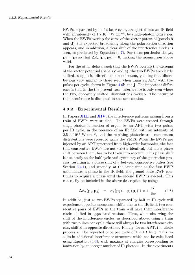
4.3.2. Experimental Results
EWPs, separated by half a laser cycle, are ejected into an IR fieldwith an intensity of 1×10¹³ W·cm−2, by single-photon ionization.When the EWPs overlap the zeros of the vector potential (panels band d), the expected broadening along the polarization directionappears, and in addition, a clear shift of the interference circles isseen, as predicted by Equation (4.7). For these particular delays,p1 = p2 so that ∆φe (p1,p2) = 0, making the assumption abovevalid.
For the other delays, such that the EWPs overlap the extremaof the vector potential (panels c and e), the two EWPs are clearlyshifted in opposite directions in momentum, yielding final distri-butions very similar to those seen when using an APT with twopulses per cycle, shown in Figure 4.6h and j. The important differ-ence is that in the the present case, interference is only seen wherethe two, oppositely shifted, distributions overlap. The nature ofthis interference is discussed in the next section.
4.3.2 Experimental Results
In Papers XIII and XIV, the interference patterns arising from atrain of EWPs were studied. The EWPs were created throughsingle-photon ionization of argon by an APT with two pulsesper IR cycle, in the presence of an IR field with an intensity of2.5 × 1013 W·cm−2, and the resulting photoelectron momentumdistributions were recorded using the VMIS. When the EWPs areinjected by an APT generated from high-order harmonics, the factthat consecutive EWPs are not strictly identical, but has a phaseshift between them, has to be taken into account. This phase shiftis due firstly to the half-cycle anti-symmetry of the generation pro-cess, resulting in a phase shift of π between consecutive pulses (seeSection 3.4.1), and secondly, at the same time as the first EWPaccumulates a phase in the IR field, the ground state EWP con-tinues to acquire a phase until the second EWP is ejected. Thiscan easily be included in the above description by using:
∆φe (p1,p2) = φe (p2)− φe (p1) + π +πIP
hω(4.8)
In addition, just as two EWPs separated by half an IR cycle willexperience opposite momentum shifts due to the IR field, two con-secutive pairs of EWPs in the train will have their interferencecircles shifted in opposite directions. Thus, when observing theshift of the interference circles, as described above, using a trainwith two pulses per cycle, there will always be two interference cir-cles, shifted in opposite directions. Finally, for an APT, the wholeprocess will be repeated once per cycle of the IR field. This re-sults in additional interference structure, which can be calculatedusing Equation (4.3), with maxima at energies corresponding toionization by an integer number of IR photons. In the experiments
64

Electron Wave Packets in External Laser Fields
px (10−24 Ns)
py
(10−
24N
s)
-2 -1 0 1 2
-2
-1
0
1
2
Figure 4.10. Experimentalmomentum distribution fromionization of argon by an APTgenerated in argon, in thepresence of an IR field with anintensity of 2.5× 10¹³ W·cm−2.The delay is such that the pulsesoverlap with the extrema of thevector potential, and the upperand lower parts of the initialmomentum distributions areshifted outside the detector.
described in Papers XIII and XIV, the shifts of the interferencecircles described above were observed, and are discussed in moredetail in Paper XIV.
Momentum-Shearing Interferometry
In Paper XIII, the interference pattern for the delay when themomentum shift is maximum, illustrated for two pulses in panels cand e of Figure 4.9, was studied more closely. In this case, thesecond term in the IR-induced phase difference [Equation (4.6)]vanishes, and the maxima of the interference pattern, pmax, canbe found by requiring the phase in Equation (4.3) to be a multipleof 2π:
π
hω
[p2
max
2m+ IP + UP
]+ φe (p2)− φe (p1) + π = 2πn (4.9)
which can be rewritten as:
p2max
2m= (2n + 1) hω − IP − UP −
hω
π[φe (p2)− φe (p1)] (4.10)
In other words, this expression states that the maxima of the inter-ference will occur for kinetic energies corresponding to ionizationby an odd number of IR photons, shifted due to the phase differ-ence between the two momentum components that overlap at thatpoint.
In the experiment, the IR field was polarized along the py-axisand the two shifted momentum distributions overlapped mainly inthe plane py = 0 (see Figure 4.9c and e), along which momentumcomponents with the same magnitude, but from opposite sides ofthe plane py = 0, are overlapped. Thus, the positions of the fringemaxima are a measure of the symmetry or anti-symmetry of thecontinuum wave packet, relative to the plane py = 0. For a wavepacket which is symmetric with respect to this plane, φe (p2) −φe (p1) = 0, and the fringes will correspond to ionization by an oddnumber of IR photons, while for an anti-symmetric wave packet,φe (p2)−φe (p1) = π, leading to peaks from ionization by an evennumber of photons.
Figure 4.10 shows the experimentally measured momentum dis-tribution. The IR field used was rather strong (2.5×10¹³ W·cm−2),so that the upper and lower parts of the distributions are shiftedoutside the detector. Still, the interference along the px-axis isclearly visible, and its maxima correspond to ionization by an evennumber of IR photons. This observation is consistent with ioniza-tion from the 3p, m = ±1 ground state in argon, resulting in ananti-symmetric continuum wave function (d,m = ±1). Furtherdetails on the data analysis, and results from TDSE calculations,can be found in Paper XIII.
65
4.3.2. Experimental Results
Finally, it should be emphasized that the method describedhere is very general, providing a tool for doing interferometryon EWPs in momentum space, in a way analogous to lateral-shearing interferometry used for the measurement of wavefrontsin optics [112]. A variant of this method has previously been sug-gested for the characterization of attosecond pulses [113], observ-ing only electrons ejected in a single direction. In principle, themethod used here, based on measuring the full momentum distri-butions, is able to measure the phase difference between any twomomentum components of the continuum wave packet that can bebrought together to interfere by the IR field. Thus, if measure-ments are made for two perpendicular polarization directions ofthe IR field, it should be possible to completely map out the phaseof the continuum wave packet, with a resolution determined by theinduced momentum shift [114].
66

Chapter 5
Summary and Outlook
Since the beginning of this thesis work, the field of attosecondphysics has seen significant advances. As attosecond pulses havebecome available in a growing number of laboratories, the tech-niques for their control and characterization have matured, andare now at the level where attosecond pulses, isolated or emittedin a train, can be routinely generated and characterized.
For APTs, important steps in their understanding and appli-cability include the first measurements of the intrinsic attosecondchirp [46], the demonstration of a direct auto-correlation measure-ment [115] and measurements of the sub-cycle timing [93, 116].
The work presented in this thesis has contributed in a numberof ways, such as through the synthesis and compression of on-targetpulses down to a duration of 170 as (Paper II) and the generationof pulse trains with a single pulse per IR cycle (Paper VI). Fromthe point of view of applications, the experiments presented inthis thesis clearly demonstrate the feasibility of using APTs as themechanism for creating EWPs for further control by an externallaser field (Papers X-XI and XIII-XIV), but also for controllingthe ionization process itself (Paper XII).
The properties of isolated attosecond pulses, synthesized fromthe cut-off region of the XUV emission from phase-stabilized few-cycle laser pulses [91], have also improved, and pulses with dura-tions of 250 as have now been measured [111]. Isolated attosecondpulses have been used so far to time resolve the emission of Augerelectrons from krypton with attosecond resolution [2], and to com-pletely map out the vector potential of a few-cycle laser pulse [117].
A third approach to attosecond physics has been to make use ofthe strong laser field directly, rather than the XUV pulses it gener-ates. One series of experiments employing this approach has beenused to study electrons from strong-field ionization by few-cycle,phase-stabilized pulses. For such short pulses, tunnel ionizationwill in principle be confined to a single half-cycle of the electric
67

field and, by controlling the carrier-envelope phase of the pulses,one can control the ionization process, and in particular the direc-tion of electron ejection, on the attosecond time-scale [100, 118]. Ina recent experiment, similar control has been demonstrated for thedissociation of a molecule [119], where asymmetry in the ejectionof the ionic fragments was observed. Another type of experimentsuses multi-cycle driving fields, and the ejected EWP itself, drivenback by the strong IR field, is used to probe its parent ion. In re-cent studies of molecular vibrations, the observable has been eitherthe fragments created through the impact between the returningEWP and the ion [120], or the high-order harmonics emitted whenthe EWP returns [121, 122]. Experiments have also been done inwhich a number of harmonic spectra have been recorded, each fora different alignment of the molecule in relation to the polarizationof the strong field. From these spectra, the molecular wave func-tion can be obtained, by using tomographic reconstruction [123].
It is safe to say that the field of attosecond physics will con-tinue to advance, and by limiting the discussion to attosecond lightpulses, it is possible to identify a few interesting points for the nearfuture. First, for the generation of APTs, the work presented inthis thesis demonstrates the flexibility that exists regarding thecentral energy, the pulse duration and even the repetition rate ofthe APTs. By finding suitable filtering mechanisms, in combina-tion with carefully chosen generating conditions, it should be pos-sible to compensate for the intrinsic chirp of the attosecond pulsesover far larger bandwidths than those presented in Paper II. Asan example, it can be mentioned that recent results from Lundshow the formation of 140 as pulses (100 as transform-limited),with a central energy of 80 eV, generated in neon and filtered byzirconium filters [60].
Another interesting development lies in the alternative schemesfor generating isolated attosecond pulses that are now starting toshow results. This is exemplified by the recent experiments pre-sented by Sola et al. [81], in which spectral measurements predictthe formation of a single attosecond pulse, using the ellipticitygating technique, also used in Paper V, to temporally confine theXUV emission from a 5 fs, phase-stabilized, IR pulse. Anotherapproach for the generation of isolated attosecond pulses is thegeneration of an APT by a two-color field, as presented in Pa-per VI. By generating an APT in this way, the repetition periodis doubled, thus relaxing the demands on the pulse duration of thedriving field [124].
Many techniques have been demonstrated for the characteri-zation of attosecond pulses, both isolated and in trains [24, 92,110, 115]. However, for APTs, the challenge of reconstructing thecomplete structure of the train from a single type of measurement([34, 95] and Papers VII and IX), still remains.
Clear applications of APTs in atomic and molecular physics
68

Summary and Outlook
emerge from the control experiments presented in Papers X-XIV.First, being synthesized from plateau harmonics, APTs provideEWPs with low kinetic energies. Thus, these are promising candi-dates for examining the effects of the atomic potential, especiallywith the results from Paper VI in mind, removing the ambiguityof having two pulses per IR cycle. Second, the results presented inPapers XIII and XIV, show the possibility of performing phasemeasurements on electronic wave functions, through interferencein the continuum EWP momentum distributions [125], using meth-ods inspired by interferometry techniques normally used in optics.
69


The Author’s Contribution tothe Papers
I Characterization of High-Order HarmonicRadiation on Femtosecond and Attosecond TimeScalesI took part in both experiments presented in this paper. Ianalyzed part of the data from the XFROG measurements.I contributed a major part to the writing of the laboratorycontrol and collection software for the RABITT measure-ments, while for the RABITT analysis, I wrote the analysisprogram and performed the analysis.
II Amplitude and Phase Control of Attosecond LightPulsesI took part in the experiment, and wrote a large part of thelaboratory control and collection software. I wrote the anal-ysis program and performed the analysis and reconstructionof the experimental data. I also took part in the writing ofthe paper.
III Experimental Studies of Attosecond Pulse TrainsI took part in some of the experiments and contributed tosome extent to the writing of the paper. I wrote the analysisprogram and performed part of the analysis.
IV Measurement and Control of the Frequency ChirpRate of High-Order Harmonic PulsesI took part in the experiment and carried out part of thedata analysis. I also contributed to the writing of the paper.
71

The Author’s Contribution to the Papers
V Time-Resolved Ellipticity Gating of High-OrderHarmonic EmissionI took part in the analysis of the experimental data, and thetheoretical comparison.
VI Attosecond Pulse Trains Generated Using TwoColor Laser FieldsI was very active in the preparation and planning of theexperiment, and also took played a major part in the ex-perimental work. I contributed to the data analysis and thewriting of the paper.
VII Probing Temporal Aspects of High-Order HarmonicPulses via Multi-Colour, Multi-Photon IonizationProcessesI played a part in the conception of the original idea andcontributed to the writing of the paper. I also wrote theSFA code used for calculating the photoelectron spectra, de-veloped the analysis program and performed the analysis.
VIII Frequency Chirp of Harmonic and AttosecondPulsesI mainly contributed through discussions and ideas prior toand during the writing of the paper. I also analyzed some ofthe experimental data and made some of the illustrations.
IX Reconstruction of Attosecond Pulse Trains Usingan Adiabatic Phase ExpansionI mainly contributed through discussions prior to and duringthe writing of the paper.
X Attosecond Electron Wave Packet Dynamics inStrong Laser FieldsI played a major part in the experiment, and wrote the lab-oratory control and collection software. I also analyzed theexperimental data and wrote the paper.
XI Trains of Attosecond Electron Wave PacketsI played a major part in the experiment, and wrote the labo-ratory control and collection software. I wrote the SFA codefor calculating the photoelectron spectra, and performed thecalculations. I also analyzed the experimental data andwrote most of the paper.
72

The Author’s Contribution to the Papers
XII Attosecond Control of Ionization DynamicsI planned and carried out the experiment. I wrote the soft-ware for the collection of ion time-of-flight data as well asthe velocity map images. I performed the analysis and wrotethe manuscript.
XIII Attosecond Electron Wave Packet InterferometryI played an essential part in the experiments and in the dis-cussions leading to the final interpretation of the results. Iwrote the camera software for collecting the velocity mapimages, and contributed to some extent to the analysis ofthe data and the writing of the paper.
XIV Angularly Resolved Electron Wave PacketInterferencesI played an essential part in the experiments and wrote thecamera software for collecting the velocity map images. Iwrote the SFA code for calculating the angular distributions,and performed the calculations. I contributed to some extentto the writing of the paper.
73

Acknowledgements
During the years of work that have resulted in this thesis, manypeople have contributed in one way or another.
First of all, I would like to thank my supervisor, AnneL’Huillier, for her genuine interest in exploring physics, and forher ability to transmit this enthusiasm to anyone working withher. My co-supervisor, Claes-Goran Wahlstrom, for always beingwilling to share his experience, practical or theoretical, throughdiscussions, often saving me a lot of work. Sune Svanberg, headof the Atomic Physics Division, for his enthusiasm when it comesto physics, but also for making the Atomic Physics Division sucha pleasant place to work at.
When I started this work in 2003, Johan Mauritsson and Ro-drigo Lopez-Martens were the people who got me going, at thesame time as we became good friends, something I am very grate-ful for. Thank you for teaching me all those clever, and also not soclever, tricks in the lab. Also, special thanks to Johan for makingall the 3D figures for this thesis.
Special thanks go to all my colleagues at the Atomic PhysicsDivision, and in particular to the fellow PhD-students and post-docs in the Attosecond Physics & High-Order Harmonic Genera-tion group: Thomas Remetter, Erik Gustafsson, Marko Swoboda,Thierry Ruchon, Olivier Guilbaud, Katalin Varju and Allan Jo-hansson. It has been a great pleasure to work with you all.
None of the experiments presented here would have workedwithout the technical support provided by Anders Persson, EmeliePourtal, Bertil Hermansson and Ake Bergquist. Also, withoutthe administrative help of Laila Lewin, Marie Holmdahl-Svensson,Britt-Marie Hansson, Minna Ramkull and Henrik Steen, thingswould have been a lot more difficult. I would also like to thankthe people at the former teaching department, in particular LarsEngstrom, Ingela Simonsson and Lennart Nilsson, for all help withthe teaching I have carried out in parallel with this work.
I have also had the privilege of collaborating with membersof groups from all over the world, who have all contributed tothe work presented in this thesis. These come from: LSU, BatonRouge, USA; CEA, Saclay, France; CELIA, Bordeaux, France;
75

Acknowledgements
FOM-AMOLF, Amsterdam, the Netherlands; LOA, Palaiseau,France; LIXAM, Orsay, France; ETH, Zurich, Switzerland andthe University of Reading, Reading, UK. Many of these collabo-rations were made possible by the support of the European Com-munity’s Improving Human Potential Programme ATTO and theMarie Curie Research Training Network XTRA. I would like tothank in particular: Ken Schafer and Mette Gaarde from LSU;Marc Vrakking from AMOLF and Pascal Salieres from CEA, forfruitful collaboration and for their hospitality when having me asa visitor.
Very special and warm thanks go to my friends and family,who have put up with a great deal during the years, but nevergave anything but more support and encouragement in return.
Finally, none of this would have been possible without the loveand support of my wife, Maria, I love you.
76

References
1. A. Zewail. Femtochemistry: Atomic-Scale Dynamics of the ChemicalBond. J. Phys. Chem. A 104, 5660 (2000).
2. M. Drescher, M. Hentschel, R. Kienberger, M. Uiberacker, V. Yakovlev,A. Scrinzi, Th. Westerwalbesloh, U. Kleineberg, U. Heinzmann andF. Krausz. Time-resolved atomic inner-shell spectroscopy. Nature 419,803 (2002).
3. A. McPherson, G. Gibson, H. Jara, U. Johann, T. S. Luk, I. A. McIn-tyre, K. Boyer and C. K. Rhodes. Studies of multiphoton production ofvacuum-ultraviolet radiation in the rare gases. J. Opt. Soc. Am. B 4,595 (1987).
4. M. Ferray, A. L’Huillier, X. F. Li, G. Mainfray and C. Manus. Multiple-harmonic conversion of 1064 nm radiation in rare gases. J. Phys. B 21,L31 (1988).
5. K. C. Kulander, K. J. Schafer and J. L. Krause. Dynamics of Short-PulseExcitation, Ionization and Harmonic Conversion. In Super-IntenseLaser-Atom Physics. Plenum Press, New York (1993).
6. K. J. Schafer, B. Yang, L. F. DiMauro and K. C. Kulander. Abovethreshold ionization beyond the high harmonic cutoff. Phys. Rev. Lett.70, 1599 (1993).
7. P. B. Corkum. Plasma perspective on strong-field multiphoton ionization.Phys. Rev. Lett. 71, 1994 (1993).
8. A. L’Huillier, M. Lewenstein, P. Salieres, Ph. Balcou, M. Yu. Ivanov,J. Larsson and C. G. Wahlstrom. High-order harmonic generation cutoff.Phys. Rev. A 48, R3433 (1993).
9. M. Lewenstein, Ph. Balcou, M.Yu. Ivanov, A. L’Huillier and P. B.Corkum. Theory of high-order harmonic generation by low-frequencylaser fields. Phys. Rev. A 49, 2117 (1994).
10. Z. Chang, A. Rundquist, H. Wang, M. M. Murnane and H. C. Kapteyn.Generation of Coherent Soft X Rays at 2.7 nm Using High Harmonics.Phys. Rev. Lett. 79, 2967 (1997).
11. Ch. Spielmann, N. H. Burnett, S. Sartania, R. Koppitsch, M. Schnurer,C. Kan, M. Lenzner, P. Wobrauschek and F. Krausz. Generation of Co-herent X-rays in the Water Window Using 5-Femtosecond Laser Pulses.Science 278, 661 (1997).
12. E. Seres, J. Seres, F. Krausz and C. Spielmann. Generation of Coher-ent Soft-X-Ray Radiation Extending Far Beyond the Titanium L Edge.Phys. Rev. Lett. 92, 163002 (2004).
77

References
13. J.-F. Hergott, M. Kovacev, H. Merdji, C. Hubert, Y. Mairesse, E. Jean,P. Breger, P. Agostini, B. Carr and P. Salires. Extreme-ultraviolet high-order harmonic pulses in the microjoule range. Phys. Rev. A 66, 021801(2002).
14. E. Takahashi, Y. Nabekawa and K. Midorikawa. Generation of 10-µJcoherent extreme-ultraviolet light by use of high-order harmonics. Opt.Lett. 27, 1920 (2002).
15. Y. Kobayashi, T. Sekikawa, Y. Nabekawa and S. Watanabe. 27-fs ex-treme ultraviolet pulse generation by high-order harmonics. Opt. Lett.23, 64 (1998).
16. T. Sekikawa, T. Ohno, T. Yamazaki, Y. Nabekawa and S. Watanabe.Pulse Compression of a High-Order Harmonic by Compensating theAtomic Dipole Phase. Phys. Rev. Lett. 83, 2564 (1999).
17. D. Descamps, L. Roos, C. Delfin, A. L’Huillier and C.-G. Wahlstrom.Two and three-photon ionization of rare gases using femtosecond har-monic pulses generated in a gas medium. Phys. Rev. A 64, 031401(2001).
18. S. L. Sorensen, O. Bjorneholm, I. Hjelte, T. Kihlgren, G. Ohrwall,S. Sundin, S. Svensson, S. Buil, D. Descamps and A. L’Huillier. Fem-tosecond pump-probe photoelectron spectroscopy of predissociative statesin acetylen. J. Chem. Phys. 112, 8038 (2000).
19. H. Merdji, P. Salieres, L. Le Deroff, J. F. Hergott, B. Carre, D. Joyeux,D. Descamps, J. Norin, C. Lynga, A. L’Huillier, C. G. Wahlstrom,M. Bellini and S. Huller. Coherence properties of high-order harmon-ics: Application to high-density laser-plasma diagnostic. Laser Part.Beams 18, 495 (2000).
20. G. Farkas and C. Toth. Proposal for attosecond light pulse generation us-ing laser induced multiple-harmonic conversion processes in rare gases.Phys. Lett. A 168, 447 (1992).
21. S. E. Harris, J. J. Macklin and T. W. Hansch. Atomic scale temporalstructure inherent to high-order harmonic generation. Opt. Commun.100, 487 (1993).
22. T. E. Glover, R. W. Schoenlein, A. H. Chin and C. V. Shank. Observa-tion of Laser Assisted Photoelectric Effect and Femtosecond High OrderHarmonic Radiation. Phys. Rev. Lett 76, 2468 (1996).
23. J. M. Schins, P. Berger, P. Agostini, R. C. Constantinescu, H. G.Muller, A. Bouhal, G. Grillon, A. Antonetti and A. Mysyrowicz. Cross-correlation measurements of femtosecond extreme-ultraviolet high-orderharmonics. J. Opt. Soc. Am. B 13, 197 (1996).
24. P. M. Paul, E. S. Toma, P. Breger, G. Mullot, F. Auge, Ph. Balcou,H. G. Muller and P. Agostini. Observation of a Train of AttosecondPulses from High Harmonic Generation. Science 292, 1689 (2001).
25. M. Hentschel, R. Kienberger, Ch. Spielmann, G. A. Reider, N. Milosevic,T. Brabec, P. Corkum, U. Heinzmannß, M. Drescher and F. Krausz.Attosecond metrology. Nature 414, 509 (2001).
26. J.-C. Diels and W. Rudolph. Ultrashort laser pulse phenomena. Aca-demic Press (1996).
27. H. Hertz. Ueber einen Einfluss des ultravioletten Lichtes auf die elec-trische Entladung. Ann. Physik 267, 983 (1887).
78
References
28. A. Einstein. Uber einen die Erzeugung und Verwandlung des Lichtesbetreffenden heuristischen Gesichtspunkt. Ann. Physik 322, 132 (1905).
29. K. C. Kulander. Time-dependent Hartree-Fock theory of multiphotonionization: Helium. Phys. Rev A 36, 2726 (1987).
30. D. J. Kennedy and S. T. Manson. Photoionization of the Noble Gases:Cross Sections and Angular Distributions. Phys. Rev. A 5, 227 (1972).
31. V. Veniard, R. Taıeb and A. Maquet. Phase dependence of (N+1) - color(N>1) ir-uv photoionization of atoms with higher harmonics. Phys.Rev. A 54, 721 (1996).
32. E. S. Toma and H. G. Muller. Calculation of matrix elements for mixedextreme-ultraviolet-infrared two-photon above-threshold ionization of ar-gon. J. Phys. B 35, 3435 (2002).
33. J. Mauritsson, M. B. Gaarde and K. J. Schafer. Accessing propertiesof electron wave packets generated by attosecond pulse trains throughtime-dependent calculations. Phys. Rev. A 72, 013401 (2005).
34. F. Quere, Y. Mairesse and J. Itatani. Temporal characterization of atto-second XUV fields. J. Mod. Opt. 52, 339 (2005).
35. P. H. Bucksbaum, R. R. Freeman, M. Bashkansky and T. J. McIlratht.Role of the ponderomotive potential in above-threshold ionization. J.Opt. Soc. Am. B 4, 760 (1987).
36. R. R. Freeman and P. H. Bucksbaum. Investigations of above-thresholdionization using subpicosecond laser pulses. J. Phys. B 24, 325 (1991).
37. V. Veniard, R. Taıeb and A. Maquet. Two-Color Multiphoton Ionizationof Atoms Using High-Order Harmonic Radiation. Phys. Rev. Lett. 74,4161 (1995).
38. H. R. Reiss. Effect of an intense electromagnetic field on a weakly boundsystem. Phys. Rev. A 22, 1786 (1980).
39. L. B. Madsen. Strong-field approximation in laser-assisted dynamics.Am. J. Phys. 73, 57 (2005).
40. P. Kruit and F. H. Read. Magnetic field paralleliser for 2π electron-spectrometer and electron-image magnifier. J. Phys. E 16, 313 (1983).
41. Andre T. J. B. Eppink and David H. Parker. Velocity map imagingof ions and electrons using electrostatic lenses: Application in photo-electron and photofragment ion imaging of molecular oxygen. Rev. Sci.Instrum. 68, 3477 (1997).
42. C. J. Dasch. One-dimensional tomography: a comparison of Abel, onion-peeling, and filtered back projection methods. Appl. Opt. 31, 1146 (1992).
43. M. J. J. Vrakking. An iterative procedure for the inversion of two-dimensional ion/photoelectron imaging experiments. Rev. Sci. Instr. 72,4084 (2001).
44. Ph. Antoine, A. L’Huillier and M. Lewenstein. Attosecond Pulse TrainsUsing High-Order Harmonics. Phys. Rev. Lett. 77, 1234 (1996).
45. J. L. Krause, K. J. Schafer and K. C. Kulander. High-order harmonicgeneration from atoms and ions in the high intensity regime. Phys. Rev.Lett. 68, 3535 (1992).
79

References
46. Y. Mairesse, A. de Bohan, L. J. Frasinski, H. Merdji, L. C. Dinu,P. Monchicourt, P. Breger, M. Kovacev, R. Taıeb, B. Carre, H. G.Muller, P. Agostini and P. Salieres. Attosecond Synchronization of High-Harmonic Soft X-rays. Science 302, 1540 (2003).
47. P. B. Corkum. Private communication (2006).
48. P. Dietrich, N. H. Brunett, M. Ivanov and P. Corkum. High-harmonicgeneration and correlated two-electron multiphoton ionization with el-liptically polarized light. Phys. Rev. A 50, 3585 (1994).
49. K. S. Budil, P. Salieres, A. L’Huillier, T. Ditmire and M. D. Perry. In-fluence of ellipticity on harmonic generation. Phys. Rev. A 48, R3437(1993).
50. Y. Liang, M. V. Ammosov and S. L. Chin. High-order harmonic gen-eration in argon by elliptically polarized picosecond dye laser pulses. J.Phys. B 27, 1269 (1994).
51. K. C. Kulander, K. J. Schafer and J. L. Krause. Time-Dependent Studiesof Multiphoton Processes. In Atoms in Intense Laser Fields. AcademicPress San Diego (1992).
52. C. Torrence and G. P. Compo. A Practical Guide to Wavelet Analysis.Bull. Am. Meteorol Soc. 79, 61 (1998).
53. M. B. Gaarde and K. J. Schafer. Quantum path distributions for high-order harmonics in rare gas atoms. Phys. Rev. A 65, 031406(R) (2002).
54. J. Tate, T. Auguste, H. G. Muller, P. Salieres, P. Agostini and L. F.DiMauro. Wave packet dynamics and attosecond chirp in mid-infraredhigh harmonic generation. Private communication (2006).
55. M. Lewenstein, P. Salieres and A. L’Huillier. Phase of the atomic po-larization in high-order harmonic generation. Phys. Rev. A 52, 4747(1995).
56. D. Strickland and G. Mourou. Compression of amplified chirped opticalpulses. Opt. Commun. 56, 219 (1985).
57. P. Maine, D. Strickland, P. Bado, M. Pessot and G. Mourou. Genera-tion of ultrahigh peak power pulses by chirped pulse amplification. IEEEJ. Quantum Electron. 24, 398 (1988).
58. D. E. Spence, P. N. Kean and W. Sibbett. 60-fsec pulse generation froma self-mode-locked Ti:sapphire laser. Opt. Lett. 16, 42 (1991).
59. P. Tournois. Acousto-optic programmable dispersive filter for adaptivecompensation of group delay time dispersion in laser systems. Opt.Commun. 140, 245 (1997).
60. E. Gustafsson, T. Ruchon, M. Swoboda, T. Remetter, R. Lopez-Martens,Ph. Balcou and A. L’Huillier. Manuscript in preparation (2006).
61. Ph. Balcou, C. Cornaggia, A. S. L. Gomes, L.-A. Lompre andA. L’Huillier. Optimizing high-order harmonic generation in strongfields. J. Phys. B 25, 4467 (1992).
62. P. Salieres, A. L’Huillier, Ph. Antoine and M. Lewenstein. Study of thespatial and temporal coherence of high-order harmonics. Adv. Atom.Mol. Opt. Phys. 41, 83 (1999).
63. P. Salieres, A. L’Huillier and M. Lewenstein. Coherence control of high-order harmonics. Phys. Rev. Lett. 74, 3776 (1995).
80
References
64. A. L’Huillier, X. F. Li and L. A. Lompre. Propagation effects in high-order harmonic generation in rare gases. J. Opt. Soc. Am. B 7, 527(1990).
65. C. Altucci, T. Starczewski, E. Mevel, C. G. Wahlstrom, B. Carre andA. LHuillier. Influence of atomic density in high-order harmonic gener-ation. J. Opt. Soc. Am. B 13, 148 (1996).
66. M. Bellini, C. Lynga, A. Tozzi, M.B. Gaarde, C. Delfin, T.W. Hansch,A. L’Huillier and C.-G. Wahlstrom. Temporal coherence of ultrashorthigh-order harmonic pulses. Phys. Rev. Lett. 81, 297 (1998).
67. H. J. Shin, D. G. Lee, Y. H. Cha, K. H. Hong and C. H. Nam. Generationof Nonadiabatic Blueshift of High Harmonics in an Intense FemtosecondLaser Field. Phys. Rev. Lett. 83, 2544 (1999).
68. C. Kan, C. E. Capjack, R. Rankin and N. H. Burnett. Spectral and tem-poral structure in high harmonic emission from ionizing atomic gases.Phys. Rev A 52, 4336 (1995).
69. I. A. Walmsley and V. Wong. Characterization of the electric field ofultrashort optical pulses. J. Opt. Soc. Am. B 13, 2453 (1996).
70. T. Sekikawa, T. Katsura, S. Miura and S. Watanabe. Measurement ofthe Intensity-Dependent Atomic Dipole Phase of a High Harmonic byFrequency-Resolved Optical Gating. Phys. Rev. Lett. 88, 193902 (2002).
71. N. A. Papadogiannis, L. A. A. Nikolopoulos, D. Charalambidis, G. D.Tsakiris, P. Tzallas and K. Witte. Two-photon ionization of He througha superposition of higher harmonics. Phys. Rev. Lett. 90, 133902 (2003).
72. T. Sekikawa, A. Kosuge, T. Kanai and S. Watanabe. Nonlinear opticsin the extreme ultraviolet. Nature 432, 605 (2004).
73. R. Trebino, K. W. DeLong, D. N. Fittinghoff, J. Sweetser, M. A.Krumbugel and B. Richman. Measuring ultrashort laser pulses in thetime-frequency domain using frequency-resolved optical gating. Rev. Sci.Instrum. 68, 1 (1997).
74. J. Norin, J. Mauritsson, A. Johansson, M. K. Raarup, A. Persson S. Buil,O. Duhr, M. B. Gaarde, K. J. Schafer, U. Keller, C.-G. Wahlstrom andA. L’Huillier. Time-Frequency Characterization of Femtosecond XUVPulses. Phys. Rev. Lett. 88, 193901 (2002).
75. R. Lopez-Martens, J. Mauritsson, A. Johansson, J. Norin andA. L’Huillier. Time-frequency characterization of high-order harmonicpulses. Eur. Phys. J. D 26, 105 (2003).
76. T. Sekikawa, T. Kanai and S. Watanabe. Frequency-Resolved OpticalGating of Femtosecond Pulses in the Extreme Ultraviolet. Phys. Rev.Lett. 91, 103902 (2003).
77. M. Nisoli, S. De Silvestri, O. Svelto, R. Szipocs, K. Ferencz, Ch. Spiel-mann, S. Sartania and F. Krausz. Compression of high-energy laserpulses below 5 fs. Opt. Lett. 22, 522 (1997).
78. C. G. Wahlstrom, J. Larsson, A. Persson, T. Starczewski, S. Svanberg,P. Salieres, Ph. Balcou and A. L’Huillier. High-order harmonic genera-tion in rare gases with an intense short-pulse laser. Phys. Rev. A 48,4709 (1993).
79. A. L’Huillier, P. Balcou, S. Candel, K. J. Schafer and K. C. Kulander.Calculations of high-order harmonic-generation processes in xenon at1064 nm. Phys. Rev. A 46, 2778 (1992).
81
References
80. P. B. Corkum, N. H. Burnett and M. Y. Ivanov. Subfemtosecond pulses.Opt. Lett. 19, 1870 (1994).
81. I. J. Sola, E. Mevel, L. Elouga, E. Constant, V. Strelkov, L. Poletto,P. Villoresi, E. Benedetti, J.-P. Caumes, S. Stagira, C. Vozzi, G. San-sone and M. Nisoli. Controlling attosecond electron dynamics by phase-stabilized polarization gating. Nature Phys. 2, 319 (2006).
82. C. Altucci, C. Delfin, L. Roos, M. Gaarde, A. L’Huillier, I. Mercer,T. Straczewski and C.-G. Wahlstrom. Frequency-resolved time-gatedhigh-order harmonics. Phys. Rev. A 58, 3934 (1998).
83. O. Tcherbakoff, E. Mevel, D. Descamps, J. Plumridge and E. Constant.Time-gated high-order harmonic generation. Phys. Rev. A 68, 0438040(2003).
84. M. Kovacev, Y. Mariesse, E. Priori, H. Merdji, O. Tcherbakoff,P. Monchieourt, P. Breger, E. Mevel, E. Constant, P. Salieres, B. Carreand P. Agostini. Temporal confinement of harmonic emission by polar-ization gating. Eur. Phys. J. D 26, 79 (2003).
85. A. Zaır, O. Tcherbakoff, E. Mevel, E. Constant, R. Lopez-Martens,J. Mauritsson, P. Johnsson and A. L’Huillier. Time-resolved measure-ments of high order harmonics confined by polarization gating. Appl.Phys. B 78, 869 (2004).
86. A. Zaır, I. J. Sola, R. Lopez-Martens, P. Johnsson, E. Cormier, K. Varju,J. Mauritsson, D. Descamps, V. Strelkov, A. L’Huillier, E. Mevel andE. Constant. Controle de la generation d’harmoniques d’ordres elevespar modulation de l’ellipticite du fondamental. J. Phys. IV France 127,91 (2005).
87. I. J. Sola, A. Zaır, R. Lopez-Martens, P. Johnsson, K. Varju, E. Cormier,J. Mauritsson, A. L’Huillier, V. Strelkov, E. Mevel and E. Constant.Temporal and spectral studies of high-order harmonics generated bypolarization-modulated infrared fields. Phys. Rev. A 74, 013810 (2006).
88. V. Strelkov, A. Zaır, O. Tcherbakoff, R. Lopez-Martens, E. Cormier,E. Mevel and E. Constant. Generation of attosecond pulses withellipticity-modulated fundamental. Appl. Phys. B 78, 879 (2004).
89. I.P. Christov, M.M. Murnane and H.C. Kapteyn. High-harmonic gener-ation of attosecond pulses in the single cycle regime. Phys. Rev. Lett.78, 1251 (1997).
90. K. J. Schafer and K. C. Kulander. High Harmonic Generation fromUltrafast Pump Lasers. Phys. Rev. Lett. 78, 638 (1997).
91. A. Baltuska, Th. Udem, M. Uiberacker, M. Hentschel, E. Goulielmakis,Ch. Gohle, R. Holzwarth, V. S. Yakovlev, A. Scrinzi, T. W. Hansch andF. Krausz. Attosecond control of electronic processes by intense lightfields. Nature 421, 611 (2003).
92. H. G. Muller. Reconstruction of attosecond harmonic beating by inter-ference of two-photon transitions. Appl. Phys. B 74, 17 (2002).
93. L. C. Dinu, H. G. Muller, S. Kazamias, G. Mullot, F Auge, Ph. Bal-cou, P. M. Paul, M. Kovacev, P. Breger and P. Agostini. Measurementof the Subcycle Timing of Attosecond XUV Bursts in High-HarmonicGeneration. Phys. Rev. Lett. 91, 063901 (2003).
82

References
94. Y. Mairesse, A. de Bohan, L. J. Frasinski, H. Merdji, L. C. Dinu,P. Monchicourt, P. Breger, M. Kovacev, T. Auguste, B. Carre, H.G.Muller, P. Agostini and P. Salieres. Optimization of Attosecond PulseGeneration. Phys. Rev. Lett. 93, 163901 (2004).
95. Y. Mairesse and F. Quere. Frequency-resolved optical gating for completereconstruction of attosecond bursts. Phys. Rev. A 71, 011401(R) (2005).
96. A.-S. Morlens, R. Lopez-Martens, O. Boyko, Ph. Zeitoun, Ph. Bal-cou, K. Varju, E. Gustafsson, T. Remetter, A. L’Huillier, S. Kazamias,J. Gautier, F. Delmotte and M.-F. Ravet. Design and characterizationof extreme-ultraviolet broadband mirrors for attosecond science. Opt.Lett. 31, 1558 (2006).
97. K. T. Kim, C. M. Kim, M.-G. Baik, G. Umesh and C. H. Nam. Single sub-50-attosecond pulse generation from chirp-compensated harmonic radi-ation using material dispersion. Phys. Rev. A 69, 051805 (2004).
98. G. G. Paulus, F. Grasbon, H. Walther, P. Villoresi, M. Nisoli, S. Stagira,E. Priori and S. De Silvestri. Absolute-phase phenomena in photoioniza-tion with few-cycle laser pulses. Nature 414, 182 (2001).
99. G. G. Paulus, F. Lindner, H. Walther, A. Baltuska, E. Goulielmakis,M. Lezius and F. Krausz. Measurement of the phase of few-cycle laserpulses. Phys. Rev. Lett. 91, 253004 (2003).
100. F. Lindner, M. G. Schatzel, H. Walther, A. Baltuska, E. Goulielmakis,F. Krausz, D. B. Milosevic, D. Bauer, W. Becker and G. G. Paulus.Attosecond Double-Slit Experiment. Phys. Rev. Lett. 95, 040401 (2005).
101. M. D. Perry and J. K. Crane. High-order harmonic emission from mixedfields. Phys. Rev. A 48 (1993).
102. H. Eichmann, A. Egbert, S. Nolte, C. Momma, B. Wellegehausen,W. Becker, S. Long, and J. K. McIver. Polarization-dependent high-order two-color mixing. Phys. Rev. A 51, R3414 (1995).
103. I. J. Kim, C. M. Kim, H. T. Kim, G. H. Lee, Y. S. Lee, J. Y. Park, D. J.Cho and C. H. Nam. Highly Efficient High-Harmonic Generation in anOrthogonally Polarized Two-Color Laser Field. Phys. Rev. Lett. 94,243901 (2005).
104. P. Agostini, F. Fabre, G. Mainfray, G. Petite and N. K. Rahman.Free-Free Transitions Following Six-Photon Ionization of Xenon Atoms.Phys. Rev. Lett. 42, 1127 (1979).
105. T. F. Gallagher. Above-Threshold Ionization in Low-Frequency Limit.Phys. Rev. Lett. 61, 2304 (1988).
106. P. B. Corkum, N. H. Burnett and F. Brunel. Above-Threshold Ionizationin the Long-Wavelength Limit. Phys. Rev. Lett. 62, 1259 (1989).
107. A. Scrinzi, M. Geissler and T. Brabec. Attosecond Cross CorrelationTechnique. Phys. Rev. Lett. 86, 412 (2001).
108. J. Mauritsson, E. Gustafsson, P. Johnsson, T. Ruchon, K. J. Schafer andA. L’Huillier. Capture and control of 3D electron motion. Manuscriptin preparation (2006).
109. E. Constant, V. D. Taranukhin, A. Stolow and P. B. Corkum. Methodsfor the measurement of the duration of high-harmonic pulses. Phys. Rev.A 56, 3870 (1997).
83

References
110. J. Itatani, F. Quere, G. L. Yudin, M. Yu. Ivanov, F. Krausz and P. B.Corkum. Attosecond Streak Camera. Phys. Rev. Lett. 88, 173903 (2002).
111. R. Kienberger, E. Goulielmakis, M. Uiberacker, A. Baltuska,V. Yakovlev, F. Bammer, A. Scrinzi, Th. Westerwalbesloh,U. Kleineberg, U. Heinzmann, M. Drescher and F. Krausz. Atomic tran-sient recorder. Nature 427, 817 (2004).
112. W. J. Bates. A wavefront shearing interferometer. Proc. Phys. Soc. 59,940–952 (1947).
113. F. Quere, J. Itatani, G. L. Yudin and P. B. Corkum. Attosecond SpectralShearing Interferometry. Phys. Rev. Lett. 90, 073902 (2003).
114. P. Johnsson, J. Mauritsson, T. Remetter, T. Ruchon, K. J. Schaferand A. L’Huillier. Phase reconstruction of electron wave packets bymomentum-shearing interferometry. Manuscript in preparation (2006).
115. P. Tzallas, D. Charalambidis, N. A. Papadogiannis, K. Witte and G. D.Tsakiris. Direct observation of attosecond light bunching. Nature 426,267 (2003).
116. S. A. Aseyev, Y. Ni, L. J. Frasinski, H. G. Muller and M. J. J. Vrakking.Attosecond Angle-Resolved Photoelectron Spectroscopy. Phys. Rev. Lett.91, 223902 (2003).
117. E. Goulielmakis, M. Uiberacker, R. Kienberger, A. Baltuska,V. Yakovlev, A. Scrinzi, Th. Westerwalbesloh, U. Kleineberg, U. Heinz-mann, M. Drescher and F. Krausz. Direct Measurement of Light Waves.Science 305, 1267 (2004).
118. A. Paul, R. A. Bartels, R. Tobey, H. Green, S. Weiman, I. P. Christov,M. M. Murnane, H. C. Kapteyn and S. Backus. Quasi-phase-matchedgeneration of coherent extreme-ultraviolet light. Nature 421, 51 (2003).
119. M. F. Kling, Ch. Siedschlag, A. J. Verhoef, J. I. Khan, M. Schultze,Th. Uphues, Y. Ni, M. Uiberacker, M. Drescher, F. Krausz and M. J. J.Vrakking. Control of Electron Localization in Molecular Dissociation.Science 312, 246 (2006).
120. H. Niikura, F. Legare, R. Hasbani, A. D. Bandrauk, M. Y. Ivanov, D. M.Villeneuve and P. B. Corkum. Sub-laser-cycle electron pulses for probingmolecular dynamics. Nature 417, 917 (2002).
121. T. Kanai, S. Minemoto and H. Sakai. Quantum interference duringhigh-order harmonic generation from aligned molecules. Nature 435,470 (2005).
122. S. Baker, J. S. Robinson, C. A. Haworth, H. Teng, R. A. Smith, C. C.Chirila, M. Lein, J. W. G. Tisch and J. P. Marangos. Probing ProtonDynamics in Molecules on an Attosecond Time Scale. Science 312, 424(2006).
123. J. Itatani, J. Levesque, D. Zeidler, Hiromichi Niikura, H. Pepin, J. C.Kieffer, P. B. Corkum and D. M. Villeneuve. Tomographic imaging ofmolecular orbitals. Nature 432, 867 (2004).
124. T. Pfeifer, L. Gallmann, M. J. Abel, D. M. Neumark and S. R. Leone.Single attosecond pulse generation in the multicycle-driver regime byadding a weak second-harmonic field. Opt. Lett. 31, 975 (2006).
125. G. L. Yudin, A. D. Bandrauk and P. B. Corkum. Chirped AttosecondPhotoelectron Spectroscopy. Phys. Rev. Lett. 96, 063022 (2006).
84

Papers


Paper ICharacterization of High-Order HarmonicRadiation on Femtosecond and Attosecond TimeScalesR. Lopez-Martens, J. Mauritsson, P. Johnsson, K. Varju,A. L’Huillier, W. Kornelis, J. Biegert, U. Keller, M. Gaarde andK. Schafer.
Appl. Phys B 78, 835 (2004).


Paper I
89

Characterization of High-Order Harmonic Radiation on Femtosecond and Attosecond Time Scales
90

Paper I
91

Characterization of High-Order Harmonic Radiation on Femtosecond and Attosecond Time Scales
92

Paper I
93

Characterization of High-Order Harmonic Radiation on Femtosecond and Attosecond Time Scales
94
Paper IIAmplitude and Phase Control of Attosecond LightPulsesR. Lopez-Martens, K. Varju, P. Johnsson, J. Mauritsson, Y. Mairesse,P. Salieres, M. B. Gaarde, K. J. Schafer, A. Persson, S. Svanberg,C.-G. Wahlstrom and A. L’Huillier.
Phys. Rev. Lett. 94, 033001 (2005).


Paper II
97

Amplitude and Phase Control of Attosecond Light Pulses
98

Paper II
99

Amplitude and Phase Control of Attosecond Light Pulses
100
Paper IIIExperimental Studies of Attosecond Pulse TrainsK. Varju, P. Johnsson, R. Lopez-Martens, T. Remetter,E. Gustafsson, J. Mauritsson, M. B. Gaarde, K. J. Schafer, Ch. Erny,I. Sola, A. Zaır, E. Constant, E. Cormier, E. Mevel and A. L’Huillier.
Laser Physics 15, 888 (2005).


Paper III
103

Experimental Studies of Attosecond Pulse Trains
104

Paper III
105

Experimental Studies of Attosecond Pulse Trains
106

Paper III
107

Experimental Studies of Attosecond Pulse Trains
108

Paper III
109

Experimental Studies of Attosecond Pulse Trains
110

Paper III
111

Experimental Studies of Attosecond Pulse Trains
112

Paper III
113


Paper IVMeasurement and Control of the Frequency ChirpRate of High-Order Harmonic PulsesJ. Mauritsson, P. Johnsson, R. Lopez-Martens, K. Varju, W. Kornelis,J. Biegert, U. Keller, M. B. Gaarde, K. J. Schafer and A. L’Huillier.
Phys. Rev. A 70, 021801 (2004).


Paper IV
117

Measurement and Control of the Frequency Chirp Rate of High-Order Harmonic Pulses
118

Paper IV
119

Measurement and Control of the Frequency Chirp Rate of High-Order Harmonic Pulses
120

Paper VTime-Resolved Ellipticity Gating of High-OrderHarmonic EmissionR. Lopez-Martens, J. Mauritsson, P. Johnsson, A. L’Huillier,O. Tcherbakoff, A. Zaır, E. Mevel and E. Constant.
Phys. Rev A 69, 053811 (2004).


Paper V
123

Time-Resolved Ellipticity Gating of High-Order Harmonic Emission
124

Paper V
125

Time-Resolved Ellipticity Gating of High-Order Harmonic Emission
126

Paper VIAttosecond Pulse Trains Generated Using TwoColor Laser FieldsJ. Mauritsson, P. Johnsson, E. Gustafsson, A. L’Huillier, K. J. Schaferand M. B. Gaarde.
Phys. Rev. Lett. 97, 013001 (2006).


Paper VI
129

Attosecond Pulse Trains Generated Using Two Color Laser Fields
130

Paper VI
131

Attosecond Pulse Trains Generated Using Two Color Laser Fields
132

Paper VIIProbing Temporal Aspects of High-OrderHarmonic Pulses via Multi-Colour, Multi-PhotonIonization ProcessesJ. Mauritsson, P. Johnsson, R. Lopez-Martens, K. Varju,A. L’Huillier, M. B. Gaarde and K. J. Schafer.
J. Phys. B 38, 2265 (2005).


Paper VII
135

Probing Temporal Aspects of High-Order Harmonic Pulses via Multi-Colour, Multi-Photon IonizationProcesses
136

Paper VII
137

Probing Temporal Aspects of High-Order Harmonic Pulses via Multi-Colour, Multi-Photon IonizationProcesses
138

Paper VII
139

Probing Temporal Aspects of High-Order Harmonic Pulses via Multi-Colour, Multi-Photon IonizationProcesses
140

Paper VII
141

Probing Temporal Aspects of High-Order Harmonic Pulses via Multi-Colour, Multi-Photon IonizationProcesses
142

Paper VII
143

Probing Temporal Aspects of High-Order Harmonic Pulses via Multi-Colour, Multi-Photon IonizationProcesses
144

Paper VII
145

Probing Temporal Aspects of High-Order Harmonic Pulses via Multi-Colour, Multi-Photon IonizationProcesses
146

Paper VII
147

Probing Temporal Aspects of High-Order Harmonic Pulses via Multi-Colour, Multi-Photon IonizationProcesses
148

Paper VIIIFrequency Chirp of Harmonic and AttosecondPulsesK. Varju, Y. Mairesse, B. Carre, M. B. Gaarde, P. Johnsson,S. Kazamias, R. Lopez-Martens, J. Mauritsson, K. J. Schafer,Ph. Balcou, A. L’Huillier and P. Salieres.
J. Mod. Opt. 52, 379 (2005).


Paper VIII
151

Frequency Chirp of Harmonic and Attosecond Pulses
152

Paper VIII
153

Frequency Chirp of Harmonic and Attosecond Pulses
154

Paper VIII
155

Frequency Chirp of Harmonic and Attosecond Pulses
156

Paper VIII
157

Frequency Chirp of Harmonic and Attosecond Pulses
158

Paper VIII
159

Frequency Chirp of Harmonic and Attosecond Pulses
160

Paper VIII
161

Frequency Chirp of Harmonic and Attosecond Pulses
162

Paper VIII
163

Frequency Chirp of Harmonic and Attosecond Pulses
164

Paper VIII
165

Frequency Chirp of Harmonic and Attosecond Pulses
166

Paper IXReconstruction of Attosecond Pulse Trains Usingan Adiabatic Phase ExpansionK. Varju, Y. Mairesse, P. Agostini, P. Breger, B. Carre,L. J. Frasinski, E. Gustafsson, P. Johnsson, J. Mauritsson, H. Merdji,P. Monchicourt, A. L’Huillier and P. Salieres.
Phys. Rev. Lett. 95, 243901 (2005).


Paper IX
169

Reconstruction of Attosecond Pulse Trains Using an Adiabatic Phase Expansion
170

Paper IX
171

Reconstruction of Attosecond Pulse Trains Using an Adiabatic Phase Expansion
172

Paper XAttosecond Electron Wave Packet Dynamics inStrong Laser FieldsP. Johnsson, R. Lopez-Martens, S. Kazamias, J. Mauritsson,C. Valentin, T. Remetter, K. Varju, M. B. Gaarde, Y. Mairesse,H. Wabnitz, P. Salieres, Ph. Balcou, K. J. Schafer and A. L’Huillier.
Phys. Rev. Lett. 95, 013001 (2005).


Paper X
175

Attosecond Electron Wave Packet Dynamics in Strong Laser Fields
176

Paper X
177

Attosecond Electron Wave Packet Dynamics in Strong Laser Fields
178

Paper XITrains of Attosecond Electron Wave PacketsP. Johnsson, K. Varju, T. Remetter, E. Gustafsson, J. Mauritsson,R. Lopez-Martens, S. Kazamias, C. Valentin, Ph. Balcou,M. B. Gaarde, K. J. Schafer and A. L’Huillier.
J. Mod. Opt. 53, 233 (2006).


Paper XI
181

Trains of Attosecond Electron Wave Packets
182

Paper XI
183

Trains of Attosecond Electron Wave Packets
184

Paper XI
185

Trains of Attosecond Electron Wave Packets
186

Paper XI
187

Trains of Attosecond Electron Wave Packets
188

Paper XI
189

Trains of Attosecond Electron Wave Packets
190

Paper XI
191

Trains of Attosecond Electron Wave Packets
192

Paper XI
193


Paper XIIAttosecond Control of Ionization DynamicsP. Johnsson, J. Mauritsson, T. Remetter, K. J. Schafer andA. L’Huillier.
Manuscript in preparation.


Paper XII
197

Attosecond Control of Ionization Dynamics
198

Paper XII
199

Attosecond Control of Ionization Dynamics
200

Paper XII
201


Paper XIIIAttosecond Electron Wave Packet InterferometryT. Remetter, P. Johnsson, J. Mauritsson, K. Varju, Y. Ni, F. Lepine,E. Gustafsson, M. Kling, J. Khan, R. Lopez-Martens, K. J. Schafer,M. J. J. Vrakking and A. L’Huillier.
Nature Physics 2, 323 (2006).


Paper XIII
205

Attosecond Electron Wave Packet Interferometry
206

Paper XIII
207

Attosecond Electron Wave Packet Interferometry
208

Paper XIVAngularly Resolved Electron Wave PacketInterferencesK. Varju, P. Johnsson, J. Mauritsson, T. Remetter, T. Ruchon, Y. Ni,F. Lepine, M. Kling, J. Khan, K. J. Schafer, M. J. J. Vrakking andA. L’Huillier.
Accepted for publication in J. Phys B.


Paper XIV
211

Angularly Resolved Electron Wave Packet Interferences
212

Paper XIV
213

Angularly Resolved Electron Wave Packet Interferences
214

Paper XIV
215

Angularly Resolved Electron Wave Packet Interferences
216

Paper XIV
217

Angularly Resolved Electron Wave Packet Interferences
218

Paper XIV
219

Angularly Resolved Electron Wave Packet Interferences
220