attribute measurement systems analysis using a binary ... · pdf fileattribute measurement...
TRANSCRIPT

AttributeAttribute MeasurementMeasurement SystemsSystemsAnalysis using A Binary Random Analysis using A Binary Random
Effects ModelEffects Model
Vahid PARTOVI NIAChair of Statistics
Swiss Federal Institute of Technology
Collaboration with: G.H. Shahkar and S.M.M. Tabatabaey
Ferdowsi University of Mashhad
Overview
IntroductionManual Method for Attribute Measurement Systems AnalysisA Binary Random Effects ModelComparison on a sample data

History
Why “attribute” measurement systems are importantHow we started the research

What is an Attribute Measurement System ?
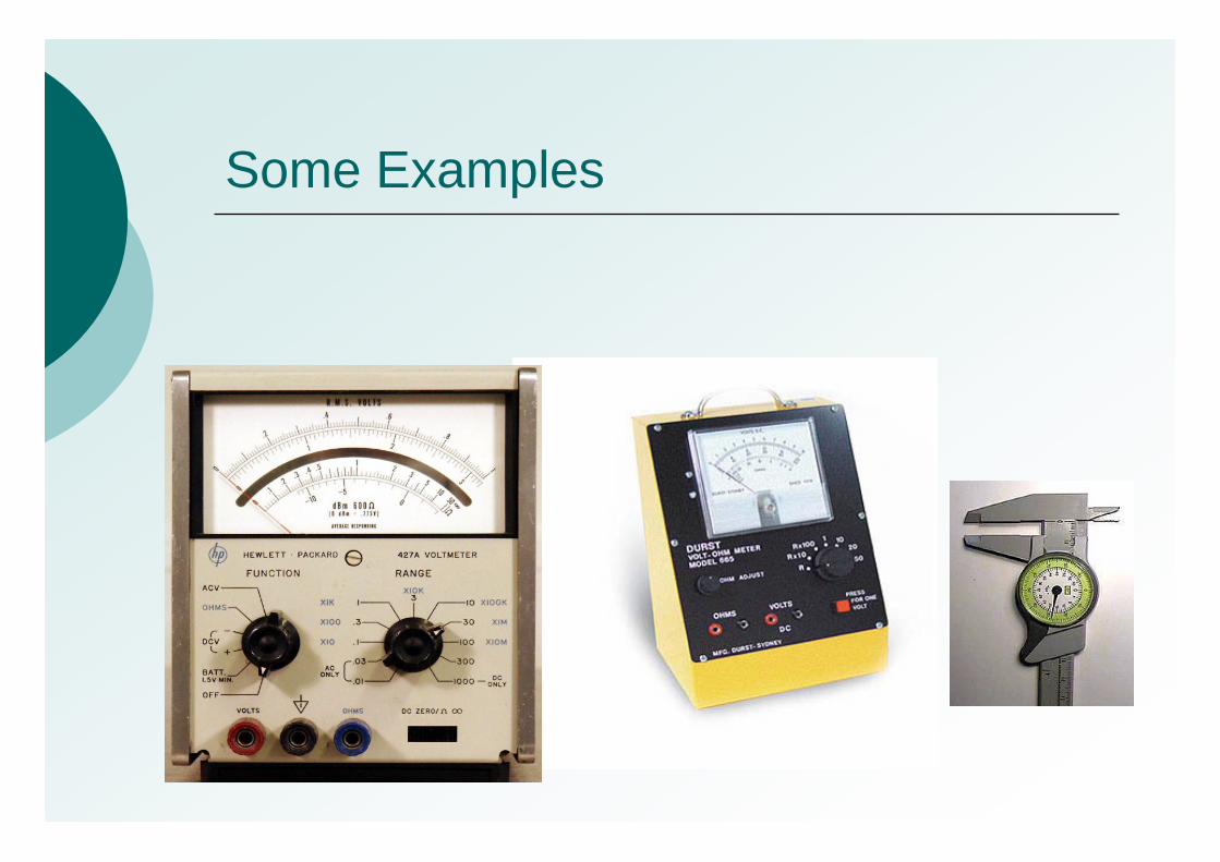
Some Examples


Types of Measurement Systems
Measurement Systems
Variable Attribute
Ruler
Calliper
X-Meter Visual Inspection Go-Nogo Gages

Properties of a Good Measurement System
RepeatabilityReproducibilityUnbiasednessNo Trend in ErrorSensitivity to The Real State

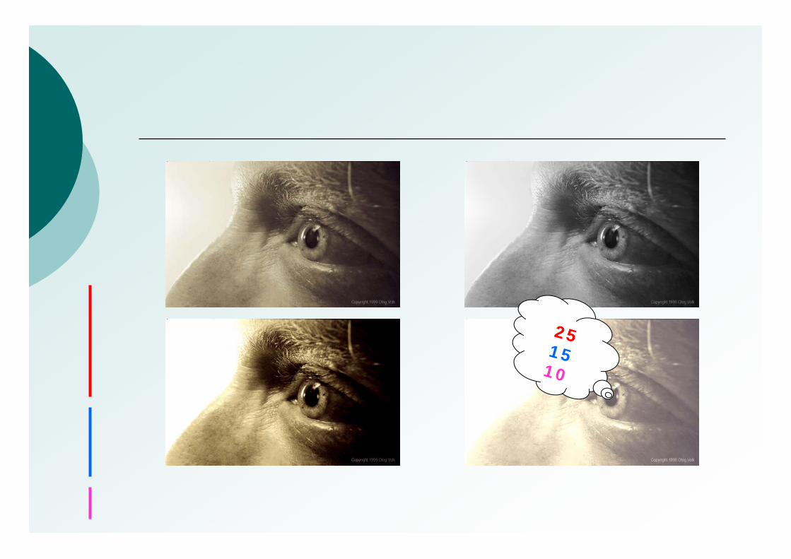
Repeatability
101525


101525


101525

251510
Reproducibility

251510

251510
251510

251510
251510
251510
251510

An R&R Measurement System
251510
251510
251510
251510


251510
251510
251510
251510


251510
251510
251510
251510
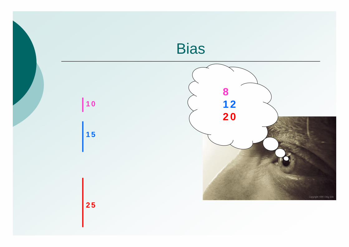
Bias
81220
10
15
25

Linearity
8 1220
10
15
25
= -2= -3= -5
REAL
2624222018161412108
ERR
OR
-1.5
-2.0
-2.5
-3.0
-3.5
-4.0
-4.5
-5.0
-5.5
REAL
2624222018161412108
Abso
lute
Err
op
5.5
5.0
4.5
4.0
3.5
3.0
2.5
2.0
1.5

251510
251510
251510
251510
25
15
10
An Ideal Measurement System

251510
251510
251510
251510
17
12
8
17128
17128
17128
17128

251510
251510
251510
251510
25
15
10

251510
251510
251510
251510
17
12
8
17128
17128
17128
17128
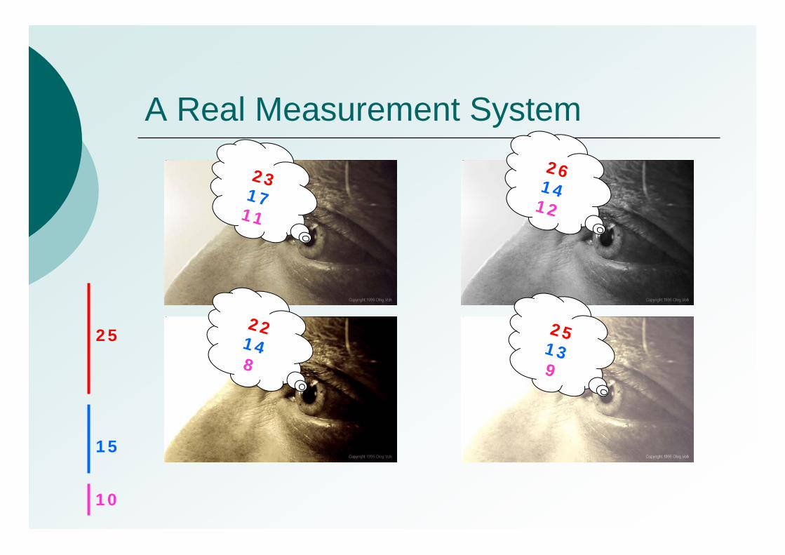
A Real Measurement System
231711
261412
22148
25139
25
15
10
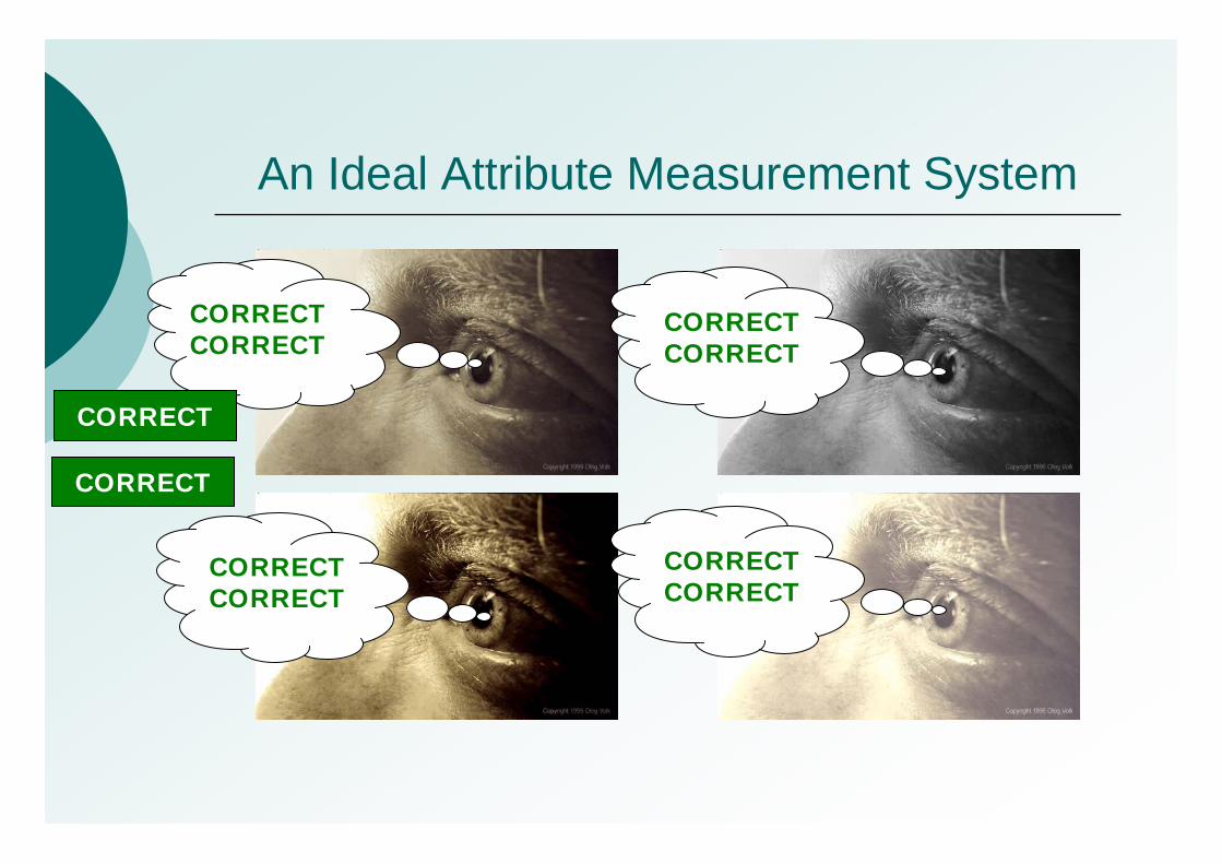
An Ideal Attribute Measurement System
CORRECTCORRECT
CORRECTCORRECT
CORRECTCORRECT
CORRECTCORRECT
CORRECT
CORRECT

An Ideal Attribute Measurement System
FAILEDCORRECT
FAILEDCORRECT
FAILEDCORRECT
FAILEDCORRECT
FAILED
FAILED
FAILEDFAILED
FAILEDFAILED
FAILEDFAILED
FAILEDFAILED
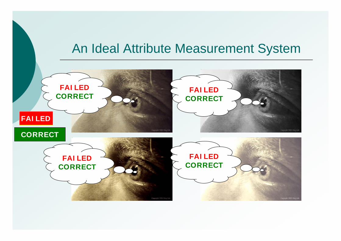
An Ideal Attribute Measurement System
FAILEDCORRECT
FAILEDCORRECT
FAILEDCORRECT
FAILEDCORRECT
FAILED
CORRECT

A Real Attribute Measurement System
CORRECTCORRECT
FAILEDCORRECT
FAILEDFAILED
CORRECTFAILED
FAILED
CORRECT

Measures of Agreement

Measures of Inter-rater Agreement
CORRECT
FAILED
CORRECT
FAILED
?
?
FALIEDCORRECT
To
tal
FA
LIE
DC
OR
RE
CT
A+B+C+D=N
A2
B+DA1
A+C
B2
C+DDC
B1
A+BBA
Rate
r B
TotalRater A
E
EO
ppp
−−
=1
κ
NCA
NBApE
+×
+=
NApO =

Agreement Based on Chance
FailedCorrect
To
tal
FailedC
orrect
N=100A2
50A1
50
B2
502525
B1
502525
Rate
B
TotalRater A
0=κ

Almost Perfect Agreement
FailedCorrect
To
tal
FailedC
orrect
N=100A2
1A1
99
B2
110
B1
99099
Rate
B
TotalRater A
99.0=κ

Almost Perfect Disagreement
FailedCorrect
To
tal
FailedC
orrect
N=100A2
99A1
1
B2
101
B1
99990
Rate
B
TotalRater A
99.0−=κ

Inadequacy of Kappa in Marginally Unbalanced Cross tabs and An Alternative
Chance Based Measure
FailedCorrect
To
tal
FailedC
orrect
N=100A2
54A1
46
B2
51456
B1
49940
Rate
B
TotalRater A
FailedCorrect
To
tal
FailedC
orrect
N=100A2
15A1
85
B2
1055
B1
901080
Rate
B
TotalRater A
32.0=κ 7.0=κ
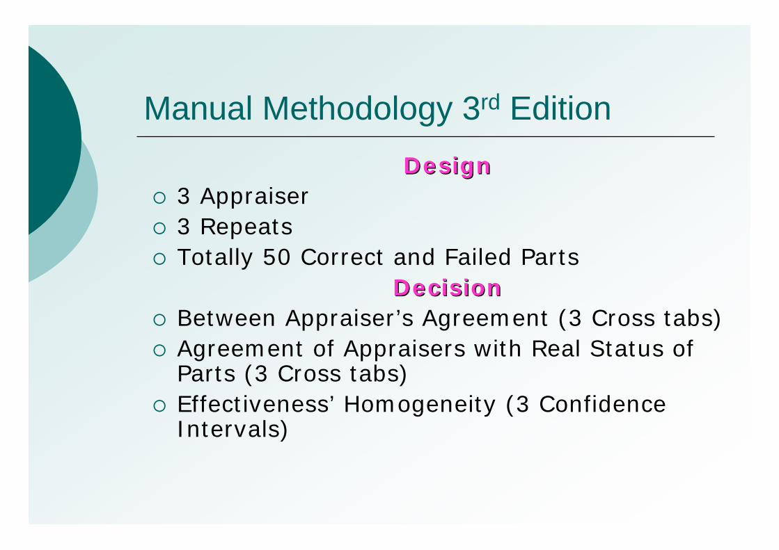
Manual Methodology 3rd EditionDesignDesign
3 Appraiser3 RepeatsTotally 50 Correct and Failed Parts
DecisionDecisionBetween Appraiser’s Agreement (3 Cross tabs)Agreement of Appraisers with Real Status of Parts (3 Cross tabs)Effectiveness’ Homogeneity (3 Confidence Intervals)

A Practical Example
Kappa0.863
976Correct
344Failed
CorrectFailedAppr. AAppr.B
Kappa0.776
927Correct
843Failed
CorrectFailedAppr. AAppr. C
Kappa0.788
945Correct942Failed
CorrectFailedAppr. BAppr.C
Kappa0.879
975Correct345Failed
CorrectFailedAppr. AREF

Continue
Kappa0.923
1002Correct
345Failed
CorrectFailedAppr. BREF
Kappa0.774
939Correct
642Failed
CorrectFailedAppr. CREF
0.690.820.74LCL0.800.900.84Score
0.910.980.94UCLAppr.A Appr.B Appr.C
http://www.carwin.co.uk/qs/english/msaamend.htm

Inadequacies of Manual Method
Kappa is not a reliable measure of agreement The error of decision is unknownSeems by adding appraisers it highly inflates type I error of overall decisionSeems to be Inconsistent!

Simulation Structure 1
Appraiser 3
Appraiser 2
Appraiser 1
Ppppppppp25Failed
Ppppppppp25Correct
321321321nState

p
Em
piric
al P
roba
bilit
y of
Rej
ecte
d M
easu
rem
ent S
yste
ms
0.5 0.6 0.7 0.8 0.9
0.0
0.2
0.4
0.6
0.8
1.0
ManualDeterministic

Simulation Structure 2
Appraiser 3
Appraiser 2
Appraiser 1
ppppppppp5Failed
ppppppppp45Correct
321321321nState

p
Em
piric
al P
roba
bilit
y of
Rej
ecte
d M
easu
rem
ent S
yste
ms
0.5 0.6 0.7 0.8 0.9
0.0
0.2
0.4
0.6
0.8
1.0
ManualDeterministic

Simulation Structure 3
Appraiser 3
Appraiser 2
Appraiser 1
0.850.85p0.850.85p0.850.85p100Failed
0.850.85p0.850.85p0.850.85p900Correct
321321321nState

P
Em
piric
al P
roba
bilit
y of
Rej
ecte
d M
easu
rem
ent S
yste
ms
0.5 0.6 0.7 0.8 0.9
0.0
0.2
0.4
0.6
0.8
1.0
DeterministicManual

Binary Random Effects Model( )( )ijiijiij
ijijijk
ROgRO
Biny
++= − µµ
µµ1,|
,1~|
ijikijijiijk ROyROy ,|,| ′⊥
ijiiij OyOy || ** ′⊥
**** ii yy ′⊥
( ) ( )[ ]( )[ ]( )∏ ∫∏ ∫
= = +++
++=
O
i
R
ijP
n
iO
n
jRn
ijiji
ijiji dFdFyROyRO
L1 1 .
.
exp1exp
µµ
θ

Approximated Likelihood
( )( ) ( )
( ) ( )( )[ ]( ) ( )( )[ ]( )
∑∑∏∑
=
===
⎪⎪
⎭
⎪⎪
⎬
⎫
⎪⎪
⎩
⎪⎪
⎨
⎧
+++
++∝
O
P
RRO
n
in
ijRO
ijRO
R
nqn
u
n
jO
nqn
v
yuRvO
yuRvO
uwvw
1
.00
.00
0
11
0
1
22exp1
22explog~
σσµ
σσµθl

Binary Threshold Model and Its Interpretation in the Nested Model
Logistic Standard~,|iid
ijiijk ROz
).,0(~
),,0(~
,,|
2
2
Rij
Oi
ijkijiijiijk
NR
NO
ROROz
σ
σ
ε++=
µ>ijkz 1=ijky
µ≤ijkz 0=ijky
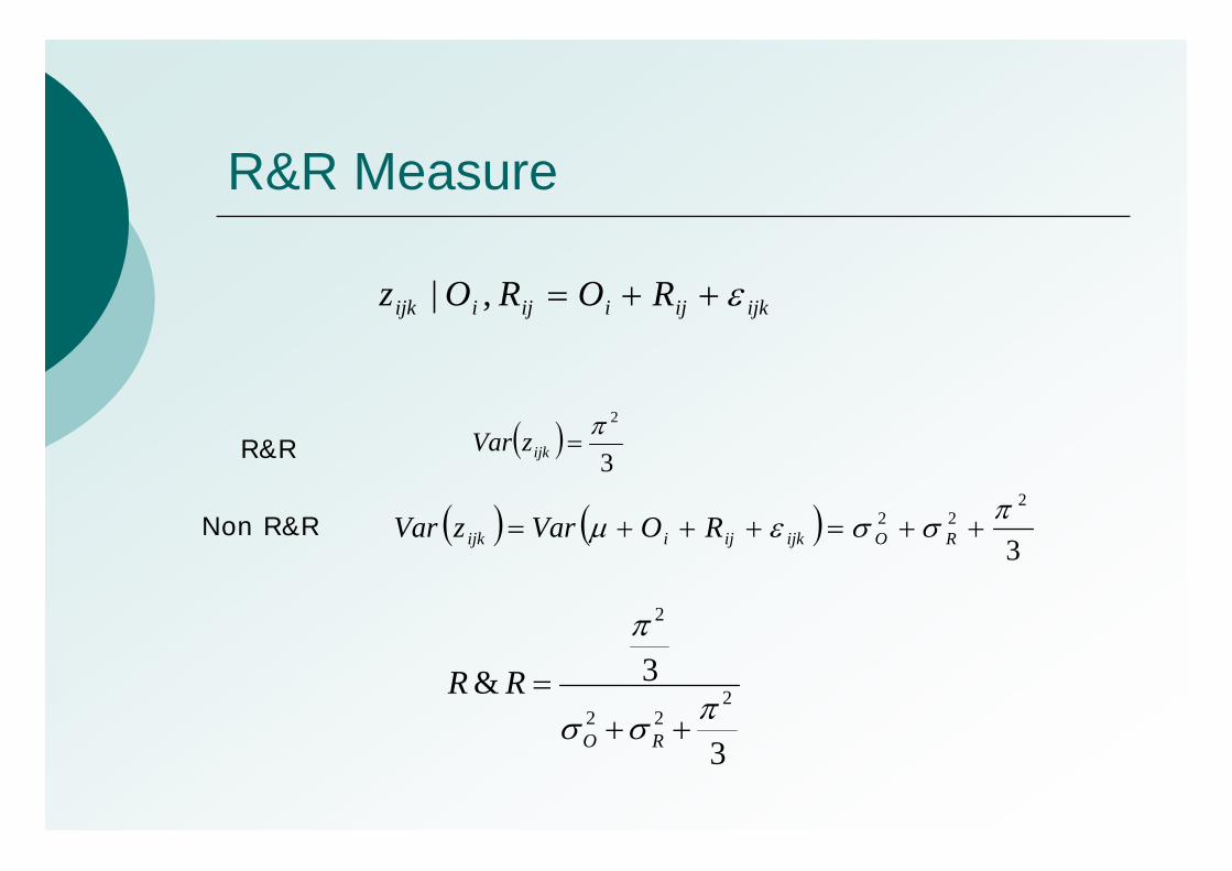
R&R Measure
( ) ( )3
222 πσσεµ ++=+++= ROijkijiijk ROVarzVar
( )3
2π=ijkzVarR&R
Non R&R
ijkijiijiijk ROROz ε++=,|
3
3& 222
2
πσσ
π
++=
RO
RR
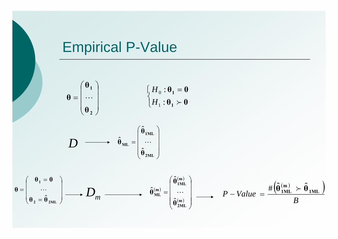
Empirical P-Value
⎟⎟⎟
⎠
⎞
⎜⎜⎜
⎝
⎛=
2
1
θ
θθ L
⎩⎨⎧ =
0θ0θ
1
1
f::
1
0
HH
⎟⎟⎟⎟
⎠
⎞
⎜⎜⎜⎜
⎝
⎛
=
2ML
1ML
ML
θ
θθ
ˆ
ˆˆ L
⎟⎟⎟
⎠
⎞
⎜⎜⎜
⎝
⎛
=
==
2ML2
1
θθ
0θθ
ˆL
D
mD ( )
( )
( ) ⎟⎟⎟⎟
⎠
⎞
⎜⎜⎜⎜
⎝
⎛
=m2ML
m1ML
mML
θ
θθ
ˆ
ˆˆ L
( )( )B
ValueP 1MLm1ML θθ ˆˆ# f
=−

Parametric Bootstrap Confidence Intervals
⎟⎟⎟
⎠
⎞
⎜⎜⎜
⎝
⎛=
2
1
θ
θθ L
⎟⎟⎟⎟
⎠
⎞
⎜⎜⎜⎜
⎝
⎛
=
2ML
1ML
ML
θ
θθ
ˆ
ˆˆ L
D ( )
( )
( ) ⎟⎟⎟⎟
⎠
⎞
⎜⎜⎜⎜
⎝
⎛
=m2ML
m1ML
mML
θ
θθ
ˆ
ˆˆ L
mD

Fitting sample data
19.0Value-P Empirical =
10 G.H. Quadrature NodesB=10000
90 % CIParameter
µ
Oσ
ORσ
( )37.3,47.2
( )48.0,0
( )1.1,0
82.0=RR

Slice likelihood
X Angle = 240 X Angle = 330
X Angle = 60 X Angle = 150
( )RO σσ ,

0.1 0.2 0.3 0.4 0.5 0.6SIGMA.O
0.2
0.6
1.0
1.4
SIG
MA
.R
-97.7 -97.5
-97.5
-97.3
-97.3
-97.2
-97.2
-97.0
-97.0
-96.8 -96.6
-96.4

One Dimensional Slice
stvec.sigmaO
mar
vec
0.02 0.04 0.06 0.08 0.10
-96.
249
-96.
247
-96.
246
-96.
244
Oσ

One Dimensional Slice
stvec.sigmaR
mar
vec
0.2 0.4 0.6 0.8 1.0 1.2 1.4
-98.
5-9
8.0
-97.
5-9
7.0
-96.
5
Rσ

One Dimensional Slice
stvec.mu
mar
vec
0 1 2 3 4 5 6
-130
-120
-110
-100
µ

Bootstrapped Distribution
-0.962784-0.351539
0.2597060.870951
1.4821972.093442
2.7046873.315932
3.9271784.538423
5.149
h0.mu.bre
0.0
0.2
0.4
0.6
0.8
1.0
1.2
µ̂

Bootstrapped Distribution
0.0000000.275758
0.5515150.827273
1.1030311.378788
1.6545461.930303
2.2060612.481819
2.757
h0.sigmaO.bre
0
1
2
3
4
5
Oσ̂

Bootstrapped Distribution
0.0000000.281217
0.5624340.843651
1.1248691.406086
1.6873031.968520
2.2497372.530954
2.8121
h0.sigmaRO.bre
0.0
0.5
1.0
1.5
2.0
2.5
Rσ̂

Summary
We discussed good properties of measurement systemsWe applied a model and responded to requirementsWe showed how Bootstrapping methods could be used where we have lack of small sample theory in GLMMs.

Thanks to
Meeting Organizers Anthony C. Davison