attrition in longitudinal household survey data · table of contents 1 introduction 80 2 some...

Demographic Research a free, expedited, online journal of peer-reviewed research and commentary in the population sciences published by the Max Planck Institute for Demographic Research Doberaner Strasse 114 · D-18057 Rostock · GERMANY www.demographic-research.org

DEMOGRAPHIC RESEARCH VOLUME 5, ARTICLE 4, PAGES 79-124 PUBLISHED 13 NOVEMBER 2001 www.demographic-research.org/Volumes/Vol5/4/ DOI: 10.4054/DemRes.2001.5.4

Attrition in Longitudinal Household Survey Data

Harold Alderman

Jere R. Behrman

Hans-Peter Kohler

John A. Maluccio

Susan Cotts Watkins

© 2001 Max-Planck-Gesellschaft.

Table of Contents

1 Introduction 80

2 Some Theoretical Aspects of the Effects ofAttrition on Estimates

82

2.1 Attrition bias due to selection on observables andunobservables

83

2.2 Testing for attrition bias 87

3 Data and Extent of Attrition 883.1 Bolivian Pre-School Program Evaluation

Household Survey Data. El Proyecto Integral deDesarrollo Infantil (PIDI)

89

3.2 The Kenyan Ideational Change Survey (KDICP) 893.3 KwaZulu-Natal Income Dynamics Study (KIDS) 90

4 Some Attrition Tests for the Bolivian, Kenyan, andSouth African Samples

92

4.1 Comparison of Means for Major Outcome andControl Variables

93

4.2 Probits for Probability of Attrition 994.3 Do Those Lost to Follow-up have Different

Coefficient Estimates than Those Re-interviewed?103

5 Conclusions 113

6 Acknowledgements 114

Notes 116

References 120

Appendix 123

Demographic Research - Volume 5, Article 4

http://www.demographic-research.org 79

Attrition in Longitudinal Household Survey Data:Some Tests for Three Developing-Country Samples

Harold Alderman 1, Jere R. Behrman 2, Hans-Peter Kohler 3, John A. Maluccio 4,

and Susan Cotts Watkins 5

Abstract

Longitudinal household data can have considerable advantages over much more widelyused cross-sectional data for capturing dynamic demographic relationships. However, adisturbing feature of such data is that there is often substantial attrition and this may makethe interpretation of estimates problematic. Such attrition may be particularly severe wherethere is considerable migration between rural and urban areas. Many analysts share theintuition that attrition is likely to be selective on characteristics such as schooling and thusthat high attrition is likely to bias estimates. This paper considers the extent andimplications of attrition for three longitudinal household surveys from Bolivia, Kenya, andSouth Africa that report very high per-year attrition rates between survey rounds. Ourestimates indicate that: (a) the means for a number of critical outcome and familybackground variables differ significantly between those who are lost to follow-up and thosewho are re-interviewed; (b) a number of family background variables are significantpredictors of attrition; but (c) nevertheless, the coefficient estimates for standard familybackground variables in regressions and probit equations for a majority of the outcomevariables considered in all three data sets are not affected significantly by attrition.Therefore, attrition apparently is not a general problem for obtaining consistent estimates

1 Development Research Group, World Bank, 1818 H Street NW, Washington D.C. 20433, USA. Email:

[email protected].

2 Population Studies Center, McNeil 160, 3718 Locust Walk, University of Pennsylvania, Philadelphia,

PA 19104-6297, USA. Email: [email protected].

3 Max-Planck Institute for Demographic Research, Doberaner Str. 114, 18057 Rostock, Germany. Email:

[email protected].

4 International Food Policy Research Institute, 2033 K Street NW, Washington D.C. 20006, USA. Email:

[email protected].

5 University of Pennsylvania, McNeil 113, 3718 Locust Walk, Philadelphia, PA 19104-6299, USA.

Email: [email protected].


80 http://www.demographic-research.org

of the coefficients of interest for most of these outcomes. These results, which are verysimilar to those for developed countries, suggest that multivariate estimates of behavioralrelations may not be biased due to attrition and thus support the collection of longitudinaldata.

1. Introduction

Longitudinal (or panel) household data can have considerable advantages over more widelyavailable cross-sectional data for social science analysis. Longitudinal data permit (1)tracing the dynamics of behaviors, (2) identifying the influence of past behaviors on currentbehaviors, and (3) controlling for unobserved fixed characteristics in the investigation ofthe effect of time-varying exogenous variables on endogenous behaviors. These advantagesare substantial for demographers studying processes that occur over time including theimpact of programs on subsequent behavior that often use time-varying exogenousvariables. As a result, the advantages are also increasingly appreciated: for example, areview of articles published in the journal Demography indicates that only 26 articles usinglongitudinal data appeared between 1980-1989, while there were 65 between 1990-2000.

Unfortunately, the collection of longitudinal data is likely to be difficult andexpensive, and some researchers, such as Ashenfelter, Deaton, and Solon (1986), havequestioned whether the gains are worth the costs. One problem in particular that hasconcerned analysts is that sample attrition may lead to selective samples and make theinterpretation of estimates problematic. Many analysts share the intuition that attrition islikely to be selective on characteristics such as schooling and thus that high attrition islikely to bias estimates made from longitudinal data. While there has been some work onthe effect of attrition on estimates using developed-country samples, little has been doneusing data from developing countries, where considerable migration between rural andurban areas typically exacerbates the problem of attrition. Table 1 summarizes the attritionrates in a number of longitudinal data sets from developing countries. While these varywidely (ranging from 6 to 50 percent between two survey rounds and 1.5 to 23.2 percentper year between survey rounds), often there is considerable attrition.In this paper, we consider some of the implications of attrition for three of the sevenlongitudinal household surveys from developing countries in Table 1 that report the highestper-year attrition rates between survey rounds: (1) a Bolivian household survey designedto evaluate an early childhood development intervention in poor urban areas, with surveyrounds in 1995/1996 and 1998; (2) a Kenyan rural household survey designed to investigatethe role of social networks in attitudes and behavior regarding reproductive health, withsurvey rounds in 1994/1995 and 1996/1997; and (3) a South African (KwaZulu-Natal



Table 1: Attrition rates for longitudinal household survey data in developingcountries listed in order of attrition rates per year

Country, time period/intervalbetween rounds (in rough orderof attrition rates per year)

Attrition ratebetween rounds(percentage)

Attrition rate peryear(percentage) Source

Bolivia (urban), 1995/6 to 1998(two-year interval) 35 19.4

Present study (alsosee Alderman andBehrman 1999)

Kenya (rural, South NyanzaProvince), 1994/5 to 1996/7(two-year interval) couplesmenwomen

413328

23.218.115.1

Present study (alsosee Behrman,Kohler, andWatkins 2001)

Nigeria (five-year interval) 50 13.0 Renne (1997)

South Africa (KwaZulu-Natal)1993 to 1998. (five yearinterval)householdspreschool children

1622

3.44.8

Present study (alsosee Maluccio2001)

India (rural) 1970/71 to 1981/2(11-year interval) 33 3.6

Foster andRosenzweig 1995

Malaysia (12-year interval) 25 2.4 Smith and Thomas1997

Indonesia 1993 to 1997 (four-year interval) 6 1.5

Thomas,Frankenberg, andSmith 1999

Note: The annual attrition rate is calculated as 1- (1-q)1/T, where q is the overall attrition rate and T is the number of years coveredby the panel.



Province) rural and urban household survey designed for more general purposes, withsurvey rounds in 1993 and 1998. The different aims of the projects and the variety ofoutcome measures facilitate generalization, at least for survey areas such as these that arerelatively poor and experiencing considerable mobility.

Drawing on recent studies on attrition in longitudinal surveys for developed countries,the next section summarizes theoretical aspects of the effects of attrition on estimates.Section 3 describes the three datasets used in this study and section 4 presents some testsfor the implications of attrition between the first and the second rounds of the three surveys.Section 5 summarizes our conclusions.

2. Some Theoretical Aspects of the Effects of Attrition on Estimates

Most of the previous work on attrition in large longitudinal samples is for developedeconomies, for example, the studies published in a special issue of The Journal of HumanResources (Spring 1998) on Attrition in Longitudinal Surveys (for related statisticalliterature on missing values and survey non-response see for instance Little and Rubin 1987or Ahlo 1990). The striking result of the studies presented in the Journal of HumanResources (JHR) is that the biases in estimated socioeconomic relations due to attrition aresmall despite attrition rates as high as 50 percent and significant differences between thosere-interviewed and those lost to follow-up for many important characteristics. For example,Fitzgerald, Gottschalk and Moffitt (1998) summarize:

By 1989 the Michigan Panel Study on Income Dynamics (PSID) had experiencedapproximately 50 percent sample loss from cumulative attrition from its initial 1968membership… (p. 251)

We find that while the PSID has been highly selective on many important variablesof interest, including those ordinarily regarded as outcome variables, attrition biasnevertheless remains quite small in magnitude. … (most attrition is random)... (p.252)

Although a sample loss as high as [experienced] must necessarily reduce precisionof estimation, there is no necessary relationship between the size of the sample lossfrom attrition and the existence or magnitude of attrition bias. Even a large amountof attrition causes no bias if it is ‘random’ … (p. 256)

The other studies in this special issue of the JHR further confirm these findings for thePSID or reach similar conclusions for other important panel data such as the Survey of



Income and Program Participation (SIPP), the National Longitudinal Surveys of Labor Market Experience (NLS), and the Labor Supply Panel Survey in the Netherlands (Falarisand Peters 1998; Lillard and Panis1998; Van den Berg and Lindeboom 1998; Zabel 1998;Ziliak and Kniesner 1998).

This absence of relevant distortions in parameter estimates due to attrition can beunderstood once the relation between the mechanisms leading to attrition and the empiricalmodel of interest is made explicit.

2.1 Attrition bias due to selection on observables and unobservables

Fitzgerald, Gottschalk, and Moffitt (1998) provide an econometric framework for theanalysis of attrition in which the common distinction between selection on variablesobserved in the data and variables that are unobserved is used to develop tests for attritionbias and correction factors to eliminate it. (Note 1) This framework assumes a panel studythat attempts to interview the same sample of respondents (or households, etc.) for say, Tannual survey rounds at times t = 1, … T. The initial sample at time t=1 is assumed to bea random or stratified random sample of the population. Attrition of a respondent at timet, denoted At, is then defined as the fact that the respondent participates in all survey waves1, …, t-1, but does not participate in any survey wave from time t onwards (Note 2).Common causes for attrition are death or migration of the respondent, or refusal toparticipate due to saturation or frustration with a particular survey. The respondent thusreports information for the dependent and explanatory variables for the survey waves 1, …,t-1. Neither the dependent variable nor time-varying explanatory variables are observedfrom survey wave t onwards. (Note 3) Analyses of and adjustments for attrition at time tcan therefore be based on fixed characteristics of the respondent, lagged time-varyingvariables pertaining to periods prior to time t, and information that do not require thecompletion of an interview, such as interviewer characteristics and location of residence.

The central concern in the analyses of attrition – and of missing data in general – isselection bias, that is, a distortion of the estimation results due to non-random patterns ofattrition. The common distinction is between attrition that is completely random, attritionthat is selective on variables unobserved in the data, and attrition that is selective onvariables observed in the data. The latter can be further distinguished between attrition thatleads to ignorable selection on observables (the statistical literature on missing data alsouses the terms “missing-at-random”) or non-ignorable selection on observables.

While attrition does not necessarily introduce bias in the estimates of interest, whenit does, selective attrition on observables is more amenable to statistical solutions thanselective attrition on unobservables. In particular, the above taxonomy of attrition leads toa sequence of tests that we will follow in this study. First, given that there is sample



attrition, one determines whether or not there is selection on observables. Second, if thereis selection on observables, one determines whether this attrition is ignorable – and thusdoes not bias the estimates of interest – or whether it is non-ignorable. In the latter case, theanalyses need to adjust for attrition since otherwise selection leads to biased inferencesabout relevant parameters. The available methods to correct for attrition on observables areoften relatively easy to implement and rely on relatively weak assumptions, in contrast tothe methods that are required in order to adjust for selection on unobservables. Whileselective attrition on unobservables potentially remains a problem even after the analysesaccount for selection on observables, using as much information as possible about selectionon observables in the panel helps to reduce the amount of residual, unexplained variationin the data due to attrition. Controlling for selection on observables thus will likely reducethe biases due to the selection on unobservables. (Note 4)

More formally, consider the survey wave at time t and assume that what is of interestis a conditional population density f(yt|xt) where yt is a scalar dependent variable and xt isan observed scalar independent variable (for illustration; in practice the extension treatingxt as a vector, which potentially includes lagged dependent variables, fixed characteristicsof the respondent, and lagged time-varying characteristics of the respondent, isstraightforward; see for instance Fitzgerald et al. 1998). In particular, we assume the linearparametric model

yt = 0 + 1xt + t,

yt observed if At = 0 (1)

where t is a mean-zero random variable, and At is an attrition indicator equal to 1 if anobservation is missing its value of yt because of attrition, and equal to zero if an observationis not missing its value of yt. For identification, we assume in this theoretical model that thevariable xt is observed for both attritors and non-attritors, as would be the case if it were atime-invariant or lagged variable, for example. The presence of attrition implies that Eq.(1) can only be estimated for respondents that are interviewed at time t, that is forobservations for which At=0 and yt is observed.

The analysis of these observed data can therefore determine the density f(yt|xt, At=0)that is conditional on xt and At=0. Additional information or restrictions are necessary inorder to infer the density of primary interest, f(yt|xt), from the observed data. That is, weseek f(yt) conditional on xt but not on At=0.

This additional information can come from the probability of attrition, Pr(At=0|yt, xt,zt), where zt is an auxiliary variable (or vector) that is assumed to be observable for all unitsbut is not included in xt. In particular, in the straightforward generalization to vectors, zt caninclude lagged values of the dependent variable (which are observed up to time t-1 forrespondents who are lost to follow-up at time t), as well as fixed characteristics of the



respondent, lagged time-varying characteristics, and variables that do not require thecompletion of an interview, such as interviewer characteristics and location of residence.(The set of respondent characteristics that can potentially be included in zt is restricted tothose characteristics that are not already included among the variables in xt.)

Linearizing the probability of attrition implies a process of the form

At* = 0 + 1xt + 2zt + t (2)

At = 1 if At* � 0

= 0 if At* < 0, (3)

where At* is a latent index and attrition occurs if this index is equal or larger to zero and t

is a mean-zero random influence on the attrition probability.Attrition can then be classified as follows (this classification differs slightly from that

proposed by Fitzgerald et al. 1998 and has a more direct relation to the statistical literatureon missing data; see also Kohler 2001):

Attrition exhibits selection on unobservables if Pr(At=0|yt, xt, zt) ��At=0|xt, zt), sothat the attrition function cannot be reduced from Pr(At=0|yt, xt, zt). In the specificparametric model in Eqs. (1 – 3), therefore, selection on unobservables occurs if vt is notindependent of t|xt, where t|xt is a shorthand notation for the error term t conditional onxt.

Attrition exhibits selection on observables if

Pr(At=0|yt, xt, zt) = Pr(At=0|xt, zt), (4)

that is, if, conditional on xt and zt, the attrition probability is independent of the dependentvariable yt and therefore of the unobserved factors entering the error term t in relation (1).

On one hand, this selection on observables is ignorable if (a) yt and zt are independentconditional on xt and At=0, or (b) the attrition function in Eq. (4) can be further reduced toPr(At=0|xt, zt) = Pr(At=0|xt), i.e., the probability of attrition is independent of the variablezt. Ignorable selection on observables implies that the linear regression of relation (1) onthe basis of the observed data on non-attritors leads to unbiased estimates of the coefficientsβ0 and β1. In this case, no specific methods are required to control or adjust for attrition.

On the other hand, selection on observables is non-ignorable when neither condition(a) nor (b) holds. In this case, standard linear regression analysis of relation (1) does notyield unbiased estimates of the coefficients β0 and β1, and alternative estimation techniquesare required that are further discussed below. Stated in terms of the parametric model inEqs. (1 – 3), ignorable selection on observables occurs if vt is independent of t|xt and (a’)zt is independent of t|xt, or (b’) the attrition does not depend on zt (i.e., 2 in Eq. 2 is zero).



Selection on observables in this parametric model is non-ignorable when neither condition(a’) nor (b’) holds.

Attrition is completely at random if the attrition function Pr(At=0|yt, xt, zt) can bereduced to Pr(At=0) and attrition neither depends on the dependent variable yt nor theobserved variables xt and zt. In our specific model, attrition is completely at random if vt isindependent of t|xt and 1 and 2 in Eq. (2) are zero.

Ordering these attrition patterns in terms of their assumptions from more restrictiveto less restrictive yields: completely random attrition < selective attrition on observables< selective attrition on unobservables. Completely random attrition is unlikely in mostpanel studies, and if it exists, it does not result in biases of parameter estimates. Attritionthat is selective on observables and unobservables, on the other hand, is probably acommon phenomenon in most panel studies, and we will briefly discuss the statisticalapproaches to overcome the biases that are potentially caused by such attrition.

Selection on unobservables is often presented as dependent on the estimation of theattrition index equation (2) (see for instance Maddala 1983 or Powell 1994 for discussionsof this approach). Identification, however, usually relies on nonlinearities in the indexequation or an exclusion restriction, i.e., the existence of a variable zt – often loosely termed“instrument” – that predicts attrition but is independent of t|xt and not included in xt. It isdifficult to rationalize most such exclusion restrictions because, for example, personalcharacteristics that affect attrition might also directly affect the outcome variable, i.e., theyshould be in xt or are correlated with t|xt. There may be some such identifying variables inthe form of variables that are external to individuals and not under their control, such ascharacteristics of the interviewer in the various rounds (Zabel 1998, Maluccio 2001).However, in the PSID and potentially also in other panel studies the interviewers areassigned on the basis of respondent characteristics, in which case this strategy is also notfeasible. In general, therefore, selection on unobservables presents an obstacle to accurateparameter estimation. Most promising, in our opinion, is therefore to test and – if necessaryadjust – for non-ignorable selection on observables by using as much information aspossible about selection in the panel. This reduces the amount of residual, unexplainedvariation due to attrition left over in the data and it lessens the scope for selection onunobservables for which few feasible statistical solutions exist.

If there is non-ignorable selection on observables, the critical variable is zt, a variablethat affects attrition propensities and that is also related to the density of yt conditional onxt due to the fact that zt is not independent of t|xt. In this sense, zt is “endogenous to yt.”Indeed, a lagged value of yt can play the role of zt if it is not in the structural relation beingestimated but is related to attrition.

Fitzgerald et al. (1998) show formally that, under the selection on observablesrestriction in Eq. (4), the complete population density f(yt|xt) can be computed from theconditional joint density of yt and zt, which we denote by g:



f(yt|xt) = ��yt, zt | xt, At=0) w(zt, xt) dzt, (5)

where

w(zt, xt) = Pr(At=0|xt) / Pr(At=0|zt, xt) (6)

are normalized weights (the proof of Eq. 5 is also given in the appendix of this paper).(Note 5) The numerator of Eq. (6) is the probability of remaining in the sample (i.e., non-attrition) conditional on xt, and the denominator is the probability of remaining in thesample conditional on zt and xt. The weights w(zt, xt) in Eq. (6) can be estimated from thedata when both xt and zt are observed. This is the case when – as we have assumed above– xt and zt contain either time-invariant or lagged time-varying characteristics of therespondent or variables that do not require a completed interview. (Note 6)

The intuition for Eqs. (5 – 6) is in the spirit of weighting (panel) observations with theinverse of the probability that an observation is included (as in stratified samples, forinstance); in the above case pertaining to attrition, this probability is replaced by thefunction of attrition probabilities in Eq. (6). Because both the weights and the conditionaldensity g are identifiable and estimable from the data, the complete-population densityf(yt|xt) is estimable as well as its moments such as the expected value Eyt = 0 + 1xt impliedby Eq. (1). This result is particularly important since it implies that in the linear model inEq. (1) the parameters 0 and 1 can be estimated without bias, despite the presence ofselective attrition on observables, via a weighted least squares regression (WLS) that usesthe weights defined in Eq. (6).

Inspection of Eqs. (5) and (6) also reveals the cases when selection on observables canbe ignored. In particular, if zt is not a determinant of attrition, the weights in Eq. (6) equalone and no attrition bias is present. If yt and zt are independent conditional on xt and At=0,the density g in Eq. (5) factors and it can again be shown that the unconditional densityf(yt|xt) equals the conditional density and there is no attrition bias.

2.2 Testing for attrition bias (Note 7)

Testing for attrition bias due to selection on unobservables is possible in econometricmodels that include the estimation of the attrition index. The identification of such modelswith panel data, however, is problematic due to the frequent lack of instruments that allowidentification. As an alternative, Fitzgerald et al. (1998) suggest that indirect tests forselection on unobservables can be made by comparisons with data sets without (or withmuch less) attrition (e.g., the Current Population Survey for comparison with the PSID in



the United States). Unfortunately, only very limited possibilities for such comparisons existfor most panels, and such comparisons are especially difficult in developing countries. Dueto this limited ability to detect selective attrition on unobservables with the datasetsexamined in this paper, we do not discuss this approach further nor do we perform thecorresponding tests.

Testing for selection bias due to selective attrition on observables, on the other hand,is possible in most panel studies and we will focus on these approaches. The two sufficientconditions that render the selection on observables through attrition ignorable are either (1)zt does not affect At or (2) zt is independent of yt conditional on xt and At=0. Specificationtests can be based on either of these two conditions. One test is simply to determinewhether candidate variables for zt (for example, lagged values of y) significantly affect At.Another test is based on Becketti, Gould, Lillard, and Welch (1988). In the BGLW test, thevalue of y at the initial wave of the survey (y1) is regressed on respondent’s characteristicsat the initial wave (x1) and on A, which denotes the event that a respondent becomes anattritor at some time during the survey (i.e., At equals one for some t in 2,…,T). The test forattrition is based on the significance of A in that equation. This test is closely related to thetest based on regressing A on x1 and y1, which is a direct estimation of the attritionprobability in Eqs. (2 – 3) in the special case when the y1 is used to represent the auxiliaryvariable zt. In fact, the direct estimation of the attrition probability and the BGLW test aresimply inverses of one another (Fitzgerald et al. 1998). (Note 8)

Clearly, if there is no evidence of attrition bias from these specification tests, thissuggests that the attrition on observables is ignorable. (Since the null-hypothesis of ourattrition tests is the absence of attrition, the fact that there is not significant evidence ofattrition bias from these specification tests is no proof that such bias does not exist. It does,however, show that the possible bias is too small to be detectable given the power of theavailable tests. This limitation is a general problem of statistical inference and not restrictedto the specification tests for attrition).

If the specification tests suggest that attrition on observables is ignorable, then thedesired information on f(yt|xt) can be directly inferred from the conditional density f(yt|xt,At=0) (under the assumption that there is no selective attrition on unobservables). If theabove tests detect non-ignorable selection on observables due to attrition, the resultingbiases in the inference of 0 and 1 in Eq. (1) can be avoided by using a weighted leastsquares methodology with the weights given in Eq. (6).

3. Data and Extent of Attrition

In this section, we describe the three data sets that we use, emphasizing the diverse relationsof interest they can address.



3.1 Bolivian Pre-School Program Evaluation Household Survey Data. El ProyectoIntegral de Desarrollo Infantil (PIDI)

PIDI is a targeted urban early child development project expected to improve thenutritional status and cognitive development of children who participate and to facilitatethe labor force participation of their caregivers. PIDI delivers child services throughchildcare centers located in the homes of local women who have been trained in childcare.The program provides food accounting for 70 percent of the children’s nutritional needs,health and nutrition monitoring, and programs to stimulate the children’s social andintellectual development. The PIDI program was designed to facilitate ongoing impactevaluation through the collection of longitudinal data.

Eligibility for PIDI at the time of the collection of the first and second rounds of datawas based on an assessment of social risk. As a result of this selection, children who attenda PIDI center are, on average, from poorer family backgrounds than children who live inthe same communities but who do not attend a PIDI center (Behrman, Cheng and Todd2001). The first PIDI evaluation data set (Bolivia 1) was collected between November 1995and May 1996 and consisted of 2,047 households. (Note 9) The follow-up survey (Bolivia2) was collected in the first half of 1998 and consisted of interviews in the 65 percent of theoriginal 2,047 households that could be located (plus an additional 3,453 households thatwere not visited in Bolivia 1). The attrition rate of 35 percent for Bolivia 1 is relativelyhigh, which raised concern about whether reliable inferences could be drawn from analysisof Bolivia 2.

3.2 The Kenyan Ideational Change Survey (KDICP)

KDICP is a longitudinal survey designed to collect information for the analysis of the rolesof informal networks in understanding change in knowledge and behavior related tocontraceptive use and prevention of AIDS. Four rural sites (sublocations) were chosen inNyanza Province, near Lake Victoria in the southwestern part of Kenya. The sites werechosen to be similar in most respects but to maximize variation along two dimensions: 1)the extent to which social networks were confined to the sublocation versus beinggeographically extended and 2) the presence or absence of a community-based distributionprogram aimed at increasing the use of family planning. Villages were selected randomlywithin each site and interviews were attempted with all ever-married women of childbearingage (15 – 49) and their husbands. The study consisted of ethnographic interviews, focusgroups, and a household survey of approximately 900 women of reproductive age and theirhusbands, and was conducted between December 1994 and January 1995 (Kenya 1). Asecond round was conducted in 1996/1997 (Kenya 2). (The surveys are described in detail



at www.pop.upenn.edu/networks). The attrition rates between the two surveys were 33percent for men, 28 percent for women, and 41 percent for couples (Table 1). (Note 10)These rates are comparable to the 35 percent reported for the Bolivian data.

Table 2 summarizes data on the reported causes of attrition for men and women asobtained from other household members for most individuals who were interviewed inKenya 1 but not in Kenya 2. (Note 11) Nyanza Province has a relatively high level ofAIDS: mortality between the surveys accounted for 18 percent of the reasons given formen’s attrition, but only half as much (10 percent) for women. For both men and womenthe leading explanation was migration, accounting for 59 percent of the reasons given forwomen and 48 percent of the reasons given for men. Because this is a patrilocal society,a significant share of this migration (over one-third) for women was associated with divorceor separation, but this was not a major factor for men. Not being found at home after atleast three visits by interviewers was the next most common explanation for attrition inKenya 2, accounting for about one-sixth of the reasons given for both men (18 percent) andwomen (16 percent). Explicitly refusing or claiming to be too busy or sick to participateaccounted for slightly smaller percentages – 16 percent for men and 11 percent for women(with most of this gender difference accounted by “other,” which is 4 percent for womenbut 0 percent for men).

3.3 KwaZulu-Natal Income Dynamics Study (KIDS)

The first South African national household survey, the 1993 Project for Statistics on LivingStandards and Development (PSLSD), was undertaken in the last half of 1993 under theleadership of the South African Labour and Development Research Unit (SALDRU) at theUniversity of Cape Town. (Note 12) This analysis uses a subset of these data comprisingAfricans and Indians living in KwaZulu-Natal Province and described further below.Unlike the special purpose household surveys for Bolivia and Kenya, the South Africansurvey was a comprehensive household survey similar to a Living Standards MeasurementSurvey (Grosh and Glewwe 2000) and collected a broad array of socioeconomicinformation from individuals and households. Among other things, it included sections onhousehold demographics, household environment, education, food and nonfoodexpenditures, remittances, employment and income, agricultural activities, health, andanthropometry (weights and heights of children aged six and under). The 1993 sample wasselected using a two-stage, self-weighting design. In the first stage, clusters were chosenproportional to population size from census enumerator districts or approximate equivalentswhen these were unavailable. In the second stage, all households in each chosen clusterwere enumerated and then a random sample selected (see PSLSD 1994 for further details).



Table 2: Reported reasons for men’s and women’s attrition in Kenyan (KDICP)survey

Men Women

Reason for attrition: Number Percentage Number Percentage

Working, moved to, orvisiting outside NyanzaProvince

Working, moved to, orvisiting elsewhere inNyanza Province

Not home

Refused

Sick or busy

Deceased

Separated, divorced, thenmoved away

Other

45

51

36

26

6

37

n/a

0

22.4

25.4

17.9

12.9

3.0

18.4

n/a

0.0

21

56

32

20

3

20

42

11

10.3

27.6

15.8

9.9

1.5

9.9

20.7

4.4

Total 201 205Note: n/a = not available

Since the 1993 survey, South Africa has undergone dramatic political, social, andeconomic change, beginning with the change of government after the first nationaldemocratic elections in 1994. With the aim of addressing a variety of policy researchquestions concerning how individuals and households were faring under this transition,African and Indian households surveyed by the PSLSD in South Africa’s most populousprovince, KwaZulu-Natal, were resurveyed from March to June, 1998, for the KIDS (seeMay et al. 2000). In this paper, the sample of 1993 PSLSD African and Indian householdsresiding in KwaZulu-Natal is referred to as South Africa 1 and those re-interviewed in 1998for the KIDS, South Africa 2.



An important aspect of the South Africa resurvey – differentiating it further from theBolivian and Kenyan longitudinal surveys – is that, when possible, the interviewer teamstracked, followed, and re-interviewed households that had moved. (Note 13) Hence, in theSouth Africa survey migration does not imply automatic attrition from the sample. Inaddition to reducing the level of attrition and allowing analysis of migration behavior,tracking and following plausibly reduced biases introduced by attrition, a claim we evaluatebelow.

In 1993, the KwaZulu-Natal sample contained 1,354 households (215 Indian and1,139 African). Of the target sample, 1,152 households (84 percent) with at least one 1993member were successfully re-interviewed in 1998 (Maluccio 2001). As in most surveys indeveloping countries, refusal rates were very low, less than 1 percent. The remaininghouseholds that could not be re-interviewed were either verified as having moved but couldnot be tracked (7 percent) or left no trace (8 percent). Had the sixty households that hadmoved but were successfully tracked not been followed, 79 percent of the target householdswould have been re-interviewed. Put another way, the tracking procedures yielded a 25percent reduction in the number of households that were lost to follow-up.

Re-interview rates were slightly higher in urban than in rural areas. Offsetting thatsuccess was a follow-up rate of 78 percent (of 215 households) for Indian households, allof which were urban. The follow-up rate for rural Africans was 83 percent (of 825households). There were no major differences in the analysis of attrition when weconsidered the rural and urban samples separately; therefore we present only the resultswhere we pooled them.

The discussion of attrition between South Africa 1 and South Africa 2 to this point hasfocused on attrition at the household level. For an analysis of individual level outcomes,however, attrition at the individual level is the relevant measure. Because a household wasconsidered to be found if at least one 1993 member was re-interviewed, individual-levelattrition for the entire sample is necessarily higher than household attrition (although thisneed not be the case for subsamples of individuals). Focusing on the sample of childrenaged 6 – 72 months for whom there is complete information on height, weight, and age in1993, for example, 78 percent of 897 children were re-interviewed as household membersin 1998, indicating one-third more attrition than at the household level. (Note 14).

4. Some Attrition Tests for the Bolivian, Kenyan, and South AfricanSamples

As noted, the attrition rates for the three samples considered here are considerable: 35percent for the Bolivian sample, from 28 percent for women to 41 percent for couples inthe Kenyan sample, and from 16 percent for households to 22 percent for pre-school



children in the South African sample. However, studies for developed countries suggest thatwhile attrition of this magnitude may be selective, it need not significantly affect estimatedmultivariate relations. To test this, we conducted three sets of tests of attrition as it relatesto observed variables in the data, using some of the tests presented by Fitzgerald,Gottschalk, and Moffitt (1998). We begin with a comparison of means, since the intuitionthat attrition is likely to bias estimates is often made on the basis of such univariatecomparisons. We then estimate probits for the probability of attrition in order to ask whatvariables predict attrition comparing univariate and multivariate estimates. Lastly, we testwhether coefficient estimates for a set of relations of interest to the objectives of the studiesdiffer for two subsamples, one that is lost to follow-up and one that is re-interviewed.

4.1 Comparison of Means for Major Outcome and Control Variables

First, we compared means for major outcome and control variables measured in the firstrounds of the respective data sets for those subsequently lost to follow-up versus those whowere re-interviewed (Tables 3, 4, and 5). Major characteristics are defined with respect tothe interests of the project for which these data were collected.

Bolivia: A number of means for those lost to follow-up differ statistically from thosewho eventually were re-interviewed: rates of severe stunting, moderate wasting, the fractionreporting that they mainly spoke Quechua at home, weight-for-age, gross motor ability testscores, fine motor ability test scores, language-audition test scores, personal-social testscores, mother’s age, father’s age, home ownership, fraction with both parents present,number of rooms in the home, number of siblings, ownership of durables, mother havingjob, and household income (Table 3). All of these observable characteristics distinguish thetwo subsamples at least at the 10 percent significance level, and show that in the first roundof the data (Bolivia 1) children who were worse off in terms of these measures were morelikely to be lost to follow-up before the second round than those who would eventually bere-interviewed. Among the fourteen predetermined parental and household level variablesin Table 3, eleven differ significantly for the two groups at least at the 10 percentsignificance level. Thus, both in terms of child development outcome variables and familybackground variables, attrition seems to be systematically more likely for children who areworse off. Such systematic differences, together with the high attrition rates, may causeconcern about what can be inferred with confidence from these longitudinal data.

Kenya: For the Kenyan data, both males and females lost to follow-up have higherschooling, more languages, and are more likely to have heard radio messages aboutcontraception and lived in households with males who received salaries (Table 4). They arealso younger and have fewer children than those who were re-interviewed. For a fewvariables the means differ significantly between these two subsamples for men but not for



women (ever-use of contraceptives, residence in the sublocation of Owich) or for womenbut not for men (want no more children, visited by community-based distribution agent,speaks Luo only, belongs to credit group or to clan welfare society, residence in thesublocation of Wakula South). On the other hand, the means do not differ for thesubsamples of either men or women for a number of characteristics (currently usingcontraceptives, heard about family planning at clinic, discussed family planning with others,number of partners in networks, primary schooling, lived outside of province, polygamoushousehold).

Therefore, it appears that attrition is selective in terms of some ‘modern’characteristics (including some of the outcome variables that these data were designed toanalyze) with selectivity more strongly related to women’s characteristics. But the meansfor many characteristics, including those for most of the indicators of social interaction, theimpact of which is central to the project for which these data were gathered, do not differsignificantly between those lost to follow-up and those re-interviewed.

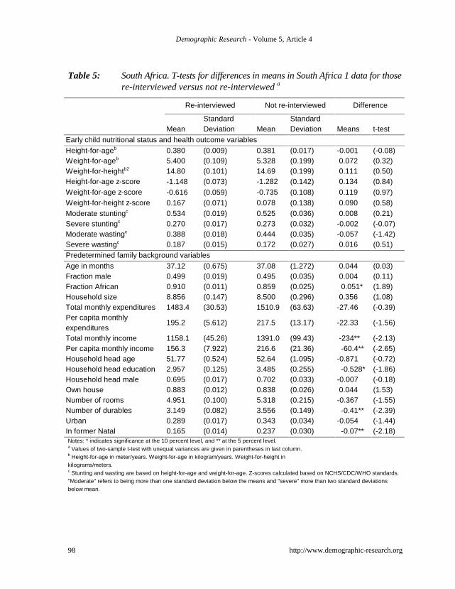
South Africa: Because the South African survey is a comprehensive household surveywith a large number of variables, for comparability this study examined a set of variablessimilar to those considered for Bolivia, i.e., measures of child nutritional status based onanthropometrics, as well as a set of predetermined family background characteristics. Theresults reported here cannot, therefore, be immediately generalized to other outcomevariables available in the South African data.

There are no significant differences in the means of child nutritional status outcomevariables between the two groups (Table 5). This is not the case for the predeterminedfamily background variables, however, where there are a number of significant differencesat the ten percent level of significance. Those pre-school children who were re-interviewedare significantly more likely to be African rather than Indian, and come from householdsthat have lower income, less educated heads, and fewer durable assets. Of course, sincethese background variables themselves tend to be highly correlated (in particular race withincome and assets), it is not surprising that they show similar patterns in the comparisonsof means. Households residing in the former Natal Province areas of the province were alsoless likely to be re-interviewed; this likely reflects higher migration, in part due to weakerproperty rights, in those areas. In sum, while there are no apparent differences in the childoutcome variables, children from better off or Indian households were more likely to be lostto follow-up.



Table 3: Bolivia. T-tests for differences in means in Bolivia 1 data for attritors versusnonattritors a

Re-interviewed Not re-interviewed Difference

Variables MeanStandardDeviation Mean

StandardDeviation Mean t-test

Early child development outcome variables

Height-for-ageb 18.0 (22.5) 17.4 (22.1) 0.65 (0.72)

Weight-for-ageb 32.2 (26.5) 30.3 (25.8) 1.91* (1.81)

Weight-for-heightb 58.1 (26.5) 56.9 (27.2) 1.21 (1.10)

Moderate stuntingc 0.639 (0.48) 0.631. (0.48) 0.008 (0.43)

Severe stuntingc 0.279 (0.45) 0.323 (0.47) -0.0437** (-2.37)

Moderate wastingc 0.365 (0.48) 0.400) (0.49 -0.035* (-1.79)

Severe wastingc 0.0796 (0.27) 0.0946 (0.29) -0.0150 (-1.30)

Gross motor ability 20.8 (7.81) 20.3 (7.67) 0.5136* (1.65)

Fine motor ability 19.4 (7.28) 19.0 (7.19) 0.480* (1.65)

Language-audition 19.2 (7.62) 18.6 (7.44) 0.569* (1.88)

Personal-social 19.9 (8.02) 19.4 (8.06) 0.534* (1.65)

Predetermined family background variables

Mother’s age 29.8 (6.45) 28.7 (6.44) 1.07** (4.10)

Father’s age 33.0 (7.70) 32.2 (8.03) 0.85** (2.66)

Mother’s schooling 3.0 (1.5) 3.0 (1.5) -0.06 (-0.9113)

Father’s schooling 3.6 (1.4) 3.6 (1.4) -0.02 (-0.42)

Quechua mainly .00099 (0.0315) 0.0114 (0.106) -0.00414** (-2.85)

Amarya mainly .00396 (0.0628) 0.00456 (0.07) -0.000605 (-0.23)

Home ownership 0.428 (0.495) 0.215 (0.411) 0.213** (12.02)

Number of rooms in house 1.50 (1.05) 1.40 (1.00) 0.100** (4.17)

Both parents present 0.841 (0.366) 0.775 (0.42) 0.0656** (4.54)

Number of siblings 2.37 (1.80) 2.05 (1.59) 0.322** (4.80)

Ownership of durablesd 6.30 (2.11) 5.92 (1.92) 0.375** (4.69)

Job of mothere 2.26 (0.91) 2.08 (0.91) 0.174** (4.73)

Job of father 2.70 (0.54) 2.70 (0.55) -0.006 (-0.28)

Household income 922 (755) 868 (638) 54** (2.68)

Notes: * indicates significance at the 10 percent level, and ** at the 5 percent level.a Values of two-sample t-test with unequal variances are given in parentheses in last column. b Height-for-age in centimeter/years. Weight-for-age in kilogram/years. Weight-for-height in kilograms/meters. c Stunting and wasting are based on height-for-age and weight-for-age. Z-scores calculated are based on CHS/CDC/WHO

standards. "Moderate" refers to being more than one standard deviation below the means and "severe" more than two standarddeviations below mean.

d Ownership of durables measures number of durables owned out of 15 asked. e Job of mother/job of father: 1=no job; 2=temporary job; 3=permanent job.



Table 4: (Men) Kenya. T-tests for differences in means in Kenya 1 data for those re-interviewed versus not re-interviewed a

Re-interviewed Not re-interviewed DifferenceMEN:



Fertility-related outcome variablesCurrently using contraceptives 0.196 (0.017) (0.031) -0.033 (-0.95)Ever used contraceptives 0.233 (0.018) 0.311 (0.052) -0.077* (-1.79)Want no more children 0.208 (0.017) 0.237 (0.031) -0.029 (-0.83)Number of surviving children 4.76 (0.171) 3.94 (0.277) 0.817** (2.46)Family planning program variablesVisited by community-based distributionagent

0.156 (0.015) 0.132 (0.025) 0.024 (0.78)

Heard family planning message on radio 0.931 (0.011) 0.968 (0.013) -0.037* (-1.86)Heard about family planning at clinic 0.495 (0.021) 0.513 (0.036) -0.018 (-0.42)Discussed with others family planning lectureheard at clinic

0.679 (0.029) 0.691 (0.047) -0.012 (-0.21)

Number of network partners in networkforFamily planning 3.7 (0.20) 4.0 (0.35) -0.3 (-0.86)Wealth flows 5.0 (0.21) 5.0 (0.36) -0.04

Reproductive health – – – (-0.10)Knows secret contraceptive user 0.637 (0.069) 0.558 (0.095) 0.079 (0.60)Control variables

Age (years) 40.1 (0.52) 36.8 (0.78) 3.3** (3.24)Education

No schooling 0.112 (0.013) 0.063 (0.018) 0.049* (1.94)

Some primary schooling 0.577 (0.021) 0.537 (0.036) 0.040 (0.96)Secondary schooling 0.298 (0.019) 0.379 (0.035) -0.081** (-2.06)

LanguageLuo only 0.796 (0.017) 0.805 (0.029) -0.010 (-0.28)English 0.443 (0.021) 0.532 (0.036) -0.089** (-2.11)Swahili 0.655 (0.020) 0.726 (0.032) -0.072* (-1.82)

Livedoutside of province 0.591 (0.021) 0.653 (0.035) 0.061 (1.49)in Nairobi or Mombasa 0.336 (0.020) 0.400 (0.036) -0.064 (-1.58)

Belongs to credit group 0.257 (0.019) 0.242 (0.031) 0.015 (0.40)Belong to clan welfare society 0.868 (0.014) 0.905 (0.021) -0.037 (-1.35)Women sell on market – – –Household characteristics

Polygamous household 0.293 (0.019) 0.238 (0.031) 0.055 (1.45)Self/Husband receives monthly salary 0.170 (0.016) 0.255 (0.032) -0.085** (-2.56)Husband interviewed – – –Household has radio – – –House has metal roof 0.173 (0.016) 0.189 (0.029) -0.016 (-0.51)

Sublocation of residenceGwassi 0.278 (0.019) 0.216 (0.030) 0.063* (1.69)Kawadhgone 0.230 (0.018) 0.237 (0.031) -0.007 (-0.20)Oyugis 0.259 (0.019) 0.300 (0.033) -0.041 (-1.11)Ugina 0.233 (0.018) 0.247 (0.032) -0.014 (-0.39)



Table 4: (continued) (Women)

Re-interviewed Not re-interviewed DifferenceWOMEN:



Fertility-related outcome variablesCurrently using contraceptives 0.126 (0.012) 0.103 (0.021) 0.024 (0.91)Ever used contraceptives 0.238 (0.016) 0.196 (0.027) 0.042 (1.25)

Want no more children 0.351 (0.018) 0.220 (0.037) 0.132** (3.59)Number of surviving children 3.88 (0.089) 2.78 (0.138) 1.10** (5.90)

Family planning program variablesVisited by community-based distributionagent

0.163 (0.014) 0.113 (0.022) 0.050* (1.75)

Heard family planning message on radio 0.870 (0.916) 0.916 (0.019) -0.046* (-1.79)Heard about family planning at clinic 0.851 (0.013) 0.828 (0.027) 0.023 (0.80)Discussed with others family planning lectureheard at clinic

0.629 (0.070) 0.661 (0.037) -0.032 (-0.76)

Number of network partners in networkforFamily planning 2.9 (0.11) 3.1 (0.20) -.18 (-0.78)Wealth flows 2.8 (0.12) 2.4 (0.21) 0.38 (1.45)Reproductive health 3.2 (0.16) 2.8 (0.23) 0.38 (1.19)

Knows secret contraceptive user 0.408 (0.02) 0.377 (0.03) 0.030 (0.77)

Control variablesAge (years) 29.7 (0.332) 26.3 (0.488) 3.4** (5.04)Education

No schooling 0.214 (0.015) 0.141 (0.024) 0.072* (2.30)Some primary schooling 0.669 (0.018) 0.668 (0.033) 0.001 (0.03)Secondary schooling 0.117 (0.012) 0.190 (0.027) -0.074** (-2.75)

LanguageLuo only 0.422 (0.018) 0.327 (0.033) 0.095* (2.46)English 0.178 (0.014) 0.263 (0.031) -0.086** (-2.73)Swahili 0.396 (0.018) 0.517 (0.035) -0.121** (-3.11)

Livedoutside of province 0.370 (0.018) 0.371 (0.034) -0.001 (-0.02)in Nairobi or Mombasa 0.214 (0.015) 0.205 (0.028) 0.009 (0.29)

Belongs to credit group 0.351 (0.018) 0.288 (0.032) 0.064* (1.70)Belong to clan welfare society 0.747 (0.016) 0.644 (0.034) 0.103** (2.93)Women sell on market 0.464 (0.019) 0.444 (0.035) 0.020 (0.51)Household characteristics

Polygamous household 0.350 (0.018) 0.371 (0.034) -0.021 (-0.56)Self/Husband receives monthly salary 0.334 (0.019) 0.402 (0.037) -0.068* (-1.66)Husband interviewed 0.765 (0.016) 0.752 (0.029) 0.013 (0.41)Household has radio 0.492 (0.019) 0.546 (0.035) -0.055 (-1.38)House has metal roof 0.201 (0.015) 0.187 (0.027) 0.014 (0.45)

Sublocation of residenceGwassi 0.213 (0.015) 0.210 (0.029) 0.003 (0.08)Kawadhgone 0.240 (0.015) 0.205 (0.028) 0.035 (1.06)Oyugis 0.286 (0.017) 0.263 (0.031) 0.023 (0.63)Ugina 0.261 (0.016) 0.322 (0.033) -0.061* (-1.72)

Note: * indicates significance at the 10 percent level, and ** at the 5 percent level. a Values of two-sample t-test with unequal variances are given in parentheses in third and sixth columns.



Table 5: South Africa. T-tests for differences in means in South Africa 1 data for thosere-interviewed versus not re-interviewed a

Re-interviewed Not re-interviewed Difference

MeanStandardDeviation Mean

StandardDeviation Means t-test

Early child nutritional status and health outcome variablesHeight-for-ageb 0.380 (0.009) 0.381 (0.017) -0.001 (-0.08)Weight-for-ageb 5.400 (0.109) 5.328 (0.199) 0.072 (0.32)Weight-for-heightb2 14.80 (0.101) 14.69 (0.199) 0.111 (0.50)Height-for-age z-score -1.148 (0.073) -1.282 (0.142) 0.134 (0.84)Weight-for-age z-score -0.616 (0.059) -0.735 (0.108) 0.119 (0.97)Weight-for-height z-score 0.167 (0.071) 0.078 (0.138) 0.090 (0.58)Moderate stuntingc 0.534 (0.019) 0.525 (0.036) 0.008 (0.21)Severe stuntingc 0.270 (0.017) 0.273 (0.032) -0.002 (-0.07)Moderate wastingc 0.388 (0.018) 0.444 (0.035) -0.057 (-1.42)Severe wastingc 0.187 (0.015) 0.172 (0.027) 0.016 (0.51)Predetermined family background variablesAge in months 37.12 (0.675) 37.08 (1.272) 0.044 (0.03)Fraction male 0.499 (0.019) 0.495 (0.035) 0.004 (0.11)Fraction African 0.910 (0.011) 0.859 (0.025) 0.051* (1.89)Household size 8.856 (0.147) 8.500 (0.296) 0.356 (1.08)Total monthly expenditures 1483.4 (30.53) 1510.9 (63.63) -27.46 (-0.39)Per capita monthlyexpenditures

195.2 (5.612) 217.5 (13.17) -22.33 (-1.56)

Total monthly income 1158.1 (45.26) 1391.0 (99.43) -234** (-2.13)Per capita monthly income 156.3 (7.922) 216.6 (21.36) -60.4** (-2.65)Household head age 51.77 (0.524) 52.64 (1.095) -0.871 (-0.72)Household head education 2.957 (0.125) 3.485 (0.255) -0.528* (-1.86)Household head male 0.695 (0.017) 0.702 (0.033) -0.007 (-0.18)Own house 0.883 (0.012) 0.838 (0.026) 0.044 (1.53)Number of rooms 4.951 (0.100) 5.318 (0.215) -0.367 (-1.55)Number of durables 3.149 (0.082) 3.556 (0.149) -0.41** (-2.39)Urban 0.289 (0.017) 0.343 (0.034) -0.054 (-1.44)In former Natal 0.165 (0.014) 0.237 (0.030) -0.07** (-2.18)Notes: * indicates significance at the 10 percent level, and ** at the 5 percent level.a Values of two-sample t-test with unequal variances are given in parentheses in last column.b Height-for-age in meter/years. Weight-for-age in kilogram/years. Weight-for-height inkilograms/meters.c Stunting and wasting are based on height-for-age and weight-for-age. Z-scores calculated based on NCHS/CDC/WHO standards."Moderate" refers to being more than one standard deviation below the means and "severe" more than two standard deviationsbelow mean.



4.2 Probits for Probability of Attrition

We start with a parsimonious specification of probits for the probability of attrition inwhich only one outcome variable at a time is included; we then include all outcomevariables plus predetermined family background variables (Table 6). The dependentvariable in these probits is whether attrition occurred between the survey rounds (1=yes;0=no)�� 2 tests for the significance of the overall relations are presented at the bottom ofTable 6.

Bolivia:�� 2 tests indicate that if only one of the outcome variables at a time isincluded in these probits, the probit is significant at the 5 percent level only for severestunting, that is, a child who is severely stunted is more likely to be lost to follow-up. Formoderate and severe low weight-for-age and the four test scores, the probits are significantat the 10 percent level, suggesting that poor childhood development is associated withhigher probability of attrition. When all of the family background variables and allchildhood development indicators are included in the analysis, however, among thechildhood development indicators only moderate stunting is significantly nonzero, even atthe 10 percent level, with a negative sign. That 1 in 11 of the childhood developmentindicators has a significant coefficient estimate at the 10 percent level in the multivariateanalysis is what one would expect to occur by chance, even if none of the childhooddevelopment indicator coefficients were truly significant predictors of attrition. Moreover,the one childhood development outcome variable that has a significantly nonzerocoefficient estimate in Table 6 in the multivariate analysis does not show significantdifferences in the comparison of means in Table 3.

The comparisons of means for childhood development outcomes between subsamplesof those lost to follow-up and those who were re-interviewed, therefore, may be misleadingregarding the extent of significant associations of these childhood development indicatorswith sample attrition once family background characteristics are controlled. Thecomparisons in Table 3 indicate that there is selective attrition with regard to childhooddevelopment indicators, with those children who are worse off in round 1 significantly morelikely to be lost to follow-up. But the multivariate estimates present a different picture: theyindicate that the extent of significant associations for the child development outcomes inprobits for predicting attrition is about what would be expected by chance. Thus,conditional on controls for observed family background characteristics, attrition is notpredicted by child development indicators for round 1. (Of course, there may bemulticollinearity among the child development indicators that disguises their significance.)

If the predetermined family background variables in Bolivia 1 are included alone orwith all of the early childhood development indicators, the probits are significantly nonzeroat very high levels. Some family background variables are significantly (at least at the 10

Dem

ographic Research - V

olume 5, A

rticle 4

100http://w

ww

.demographic-research.org

Table 6:

Probits for predicting attrition betw

een rounds 1 and 2 for Bolivian, K

enyan,and South A

frican data a

All outcome

variables

+ pre-

determined

variablese

1.204

(1.30)

0.040

(1.02)

-0.082

(-1.20)

0.297*

(1.67)

-0.144

(-0.95)

-0.036

(-0.33)

0.005

(0.03)

-0.989

(-0.72)

6.67

[0.464]

Outcome

variables,

one at a time

0.016

(0.09)

-0.009

(-0.45)

-0.005

(-0.34)

0.136

(1.25)

-0.062

(-0.52)

-0.019

(-0.21)

0.007

(0.06)

i

South Africa

Outcome

variables

Height-for-

age

Weight-for-

height

Weight-for-

age

Moderate

wasting

Severe

wasting

Moderate

stunting

Severe

stunting

All outcome

variables

+ pre-

determined

variablesd

0.004

(0.02)

-0.036

(0.28)

-0.010

(0.07)

-0.136**

(3.73)

-0.010

(0.56)

-0.097

(0.29)

54.49

[0.001]

Kenyan Women

Outcome

variables,

one at a time

-0.134

(0.92)

-0.142

(1.26)

-0.374**

(3.60)

-0.139**

(5.82)

0.012

(0.78)

h

All outcome

variables +

pre-determined

variablesc

-0.065

(0.34)

-0.103

(-0.70)

0.245*

(1.69)

-0.017

(-0.78)

0.003

(0.22)

-0.239

(-0.70)

25.13

[0.068]

Outcome

variables,

one at a

time

0.118

(0.95)

0.162*

(1.67)

0.099

(0.83)

-0.033**

(-2.46)

-0.009

(-0.85)

g

Kenyan Men

Outcome

variables

Currently

contracepting

Ever used

contraceptives

Want no more

children

Number of

surviving

children

Number of

family planning

network

partners

All outcome

variables

+ pre-

determined

variablesb

-.0002

(-0.04)

.0032

(0.80)

-.0037

(-0.78)

.1003

(0.70)

.1353

(0.70)

-.291*

(-1.93)

.2066

(1.51)

.0123

(0.59)

-.0073

(-0.35)

-.0059

(-0.27)

-.0014

(-0.07)

0.75*

(1.72)

300.22

[0.001]

Bolivia

Outcome

variables,

one at a

time

-.0015

(-0.83)

-.0015

(-0.99)

-.003*

(-1.74)

.148*

(1.78)

.191

(1.35)

-.0315

(-0.38)

.2110**

(2.41)

-.009

(-1.64)

-.009

(-1.63)

-.010*

(-1.84)

-.008

(-1.64)

f

Outcome

variables

Height-for-

age

Weight-for-

height

Weight-for-

age

Moderate

wasting

Severe

wasting

Moderate

stunting

Severe

stunting

Bulk motor

ability

Fine motor

ability

Language-

audition

Personal-

social

Constant

2test

[ S U R E � ! � 2]



Table 6: (notes)

Note: * indicates significance at the 10 percent level, and ** indicates significance at the 5 percent level.a Values of z-tests are in parentheses beneath point estimates. P-values of Chi-square tests are in brackets.b Predetermined variables for Bolivian households that are: (a) significant at 5 percent level (with sign in parentheses)—father’s

age(+); Quechua only (+); ownership of house (-); number of durables owned (-); Oruro (-), Postosi (-), Santa Cruz (-) relative toLa Paz; mother’s job permanent relative to no job (-); (b) significant at the 10 percent level – father’s schooling (-), number ofrooms in the house (+), number of siblings of child (-); father’s job temporary relative to no job (-); (c) not significant even at the10 percent level – mother’s age, mother’s schooling, Amarya only, El Alto, Cochabamba, Tarija relative to La Paz; father’s jobpermanent relative to no job; mother’s job temporary relative to no job; household income.

c Predetermined variables for Kenyan men that are (a) significant at the 5 percent level (with sign in parentheses)—men’s age; (b)not significant even at the 10 percent level – primary schooling; secondary schooling; Luo only; English; lived in Nairobi orMombasa; polygamous household; earns a monthly salary; sublocation of residence.

d Predetermined variables for Kenyan women that are: (a) significant at the 5 percent level (with sign in parentheses)—husbandinterviewed (-); (b) significant at the 10 percent level—resided in Oyugnis relative to Ugina (-) (c) not significant even at the 10percent level—primary schooling; secondary schooling; Luo only; English; lived in Nairobi or Mombasa; polygamoushousehold; household has radio; household has metal roof; other sublocation of residence.

e Predetermined variables for South African households that are (a) significant at the 5 percent level (with sign in parentheses)—age of household head(+); (b) significant at the 10 percent level—none; (c) not significant even at the 10 percent level—malechild; African household; household size; ln total monthly expenditures; household head schooling; male household head; ownthe house; number of rooms; number of durables; urban; former Natal.

I�)RU�%ROLYLDQ�GDWD��3UREDELOLW\�!� ��D��DW�WKH��SHUFHQW�OHYHO²VHYHUH�VWXQWLQJ��E��DW�WKH��SHUFHQW�OHYHO²ZHLJKW�IRU�DJH�

moderate wasting, language-auditory.J�)RU�.HQ\DQ�PHQ��3UREDELOLW\�!� ��D��DW�WKH��SHUFHQW�OHYHO²QXPEHU�RI�VXUYLYLQJ�FKLOGUHQ��E��DW�WKH��SHUFHQW�OHYHO²HYHU�XVHG

contraceptives.K�)RU�.HQ\DQ�ZRPHQ��3UREDELOLW\�!� ��D��DW�WKH��SHUFHQW�OHYHO²ZDQW�QR�PRUH�FKLOGUHQ��QXPEHU�RI�VXUYLYLQJ�FKLOGUHQ�

i��)RU�6RXWK�$IULFDQ�GDWD��3UREDELOLW\�!� 2 (a) at the 5 percent level—none; (b) at the 10 percent level—none.



percent level) associated with higher probability of attrition: older and less-schooledfathers, speaking mainly Quechua in the household, not owning the home, having morerooms in the house, having fewer siblings, having fewer durables, father having permanentor no (rather than a temporary) job, and mother having no or a temporary (rather than apermanent) job, with some significant differences also among the urban areas included inthe program. The majority of these significant coefficient estimates are consistent with whatmight be predicted from the significant differences in the means in Table 3, reinforcing theobservation that attrition tends to be selectively greater among children from worse-offfamily backgrounds.

But some of these significant coefficient estimates are opposite in sign from whatmight be expected from the comparisons of the means in Table 3, suggesting the oppositerelation to attrition if there are multivariate controls for standard background variablesother than what appear in the comparisons of means. Specifically, the comparisons in Table3 suggest that attrition is significantly more likely if fathers are younger, the house hasfewer rooms, and there are fewer siblings, but all three of these signs are reversed withsignificant coefficient estimates in the multivariate analyses of Table 6. Moreover, twovariables that are not significantly different for the two subsamples in Table 3 havesignificant coefficient estimates in Table 6, i.e., father’s schooling and father having atemporary job, both of which are estimated to significantly reduce attrition probabilities inTable 6. Finally, both mother’s age and household income have means that are significantlydifferent between the subsamples in the univariate comparisons in Table 3, but do not havecoefficient estimates that are significantly nonzero, even at the 10 percent level, once thereis control for other family background characteristics in Table 6.

Thus, exactly which family background characteristics predict attrition withmultivariate controls and what the directions of those effects are cannot be inferred simplyby examining the significance of means in univariate comparisons between the subsamples.While the patterns in Tables 3 and 6 suggest that worse-off family background is associatedwith greater attrition, the multivariate estimates are less supportive of this conclusion.

Kenya: Since there are gender differences in the probit estimates of the probability ofattrition, we report separately for men and women (Table 6). For men, we find that whenthe five outcomes are included singly, only the number of surviving children is significantlyrelated to attrition at the 5 percent level; one other – ever-used family planning – issignificantly related to attrition at the 10 percent level. If other right-side variables areincluded, among the five fertility related outcomes none is significantly nonzero at the 5percent level, and only not wanting more children is significantly related to attrition at the� �� 2 test for the joint significance of these five variables rejects suchsignificance (p=0.52). Among the control variables only age is significant, but notschooling, language, household characteristics, past residence in Nairobi or Mombasa, or



current �� 2 test for the joint significance of all the right-sidevariables rejects such significance at the 5 percent level (p=0.068).

For women, we find that two of the lagged outcome variables, wanting no morechildren and the number of surviving children, are individually significant (and negative).When all the lagged outcome variables and the predetermined variables are included, onlythe latter (number of surviving children) remains significant. However, in contrast to the�� 2 tests for the joint significance of the five fertility related outcomevariables and for the entire set of right-side variables indicate significance (p < 0.0001 inboth cases).

Thus, for the Kenyan data, there is no significant association between attrition, mostof the outcome variables, and most of the major control variables. However, gender doesmatter in these multivariate analyses: there is a significant negative association betweenattrition and number of surviving children for women but not for men.

South Africa: Probit estimates for the probability of attrition reveal little evidence thatthe outcome variables are associated with attrition of pre-school children, paralleling theresults of the mean comparisons presented in Section 4.1. When only one outcome variableat a time is included, none is significant at conventional levels. When the set of outcomevariables are included at the same time, all but moderate wasting are insignificant and a �� 2 test indicates that the set of all outcome variables together is insignificant.Moreover, the overall relation is insignificant – this set of background characteristics andoutcome variables does a very poor job predicting attrition in the sample. Thus, for theSouth African data, there is no significant association between attrition of pre-schoolchildren, most of the outcome variables, and most of the major control variables.

4.3 Do Those Lost to Follow-up have Different Coefficient Estimates than ThoseRe-interviewed?

Our aim here is to determine whether those who subsequently leave the sample differ intheir initial behavioral relationships. We conduct the BGLW tests, in which the value of anoutcome variable at the initial wave of the survey is regressed on predetermined variablesfor the initial survey wave and on subsequent attrition. In short, the test is whether thecoefficients of the predetermined variables and the constant differ for those respondentswho are subsequently lost to follow- up versus those who are re-interviewed. Tables 7, 8,and 9 present these multivariate regression and probit estimates for the same outcomevariables considered above, with the same family background variables as controls. Thefirst part of each table gives the coefficient estimates for the family background variablesfor the subsample of those who were re-interviewed. At the bottom of each table are the F�� 2 tests (for ordinary least squares regression or probit, respectively) for whether there



are significant differences between the two subsamples that test for equality of (i) all of theslope coefficients and the constant and (ii) all of the slope coefficients (but not theconstant).

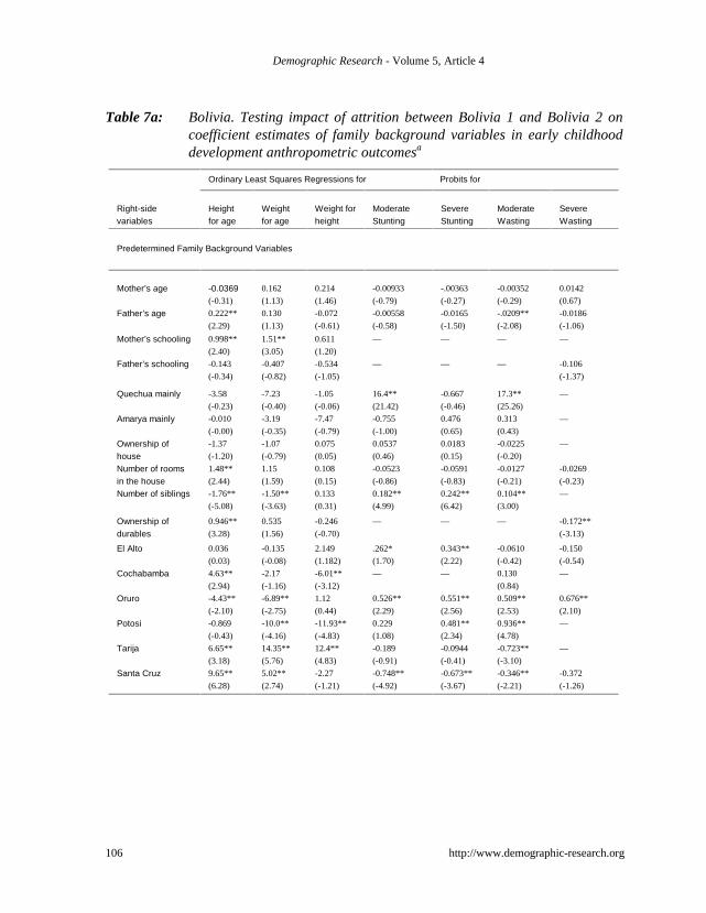
Bolivia: F tests indicate that all of the eleven estimated equations for childhooddevelopment indicators are statistically significant with a p-value of p < 0.0001 (Table 7).These estimates indicate a number of associations that are consistent with widely heldperceptions about child development. For example, household income is significantlypositively associated with height-for-age and significantly negatively associated with severestunting; mother’s schooling is significantly positively associated with height-for-age andweight-for-age, though significantly negatively associated with gross motor ability; andownership of consumer durables is significantly positively associated with height-for-age,gross motor ability, fine motor ability, language-audition, and personal-social test scores,but significantly negatively associated with severe wasting.

There are, however, no significant differences at the 5 percent level (Note 15) betweenthe set of coefficients for the subsample of those lost to follow-up versus the subsample ofthose re-interviewed for over half of the indicators of child development: height-for-age,moderate stunting, gross motor ability tests, fine motor ability tests, language-audition tests,and personal-social tests. The second set of tests, further, indicates that there are nosignificant differences at the 10 percent level for severe stunting. These estimates for theanthropometric indicators related to stunting and for the four cognitive development testscores, therefore, suggest that the coefficient estimates of standard family backgroundvariables are not significantly affected by sample attrition.

The results differ sharply, however, for the anthropometric indicators related towasting. Both tests for these four child outcome variables indicate that the coefficientestimates for observed family background variables do differ significantly at the 5 percentlevel (and for all but weight-for-age at the 1 percent level) between the two subsamples. Forthese outcomes, therefore, it is important to control for the attrition in the analysis, e.g., aswith the matching methods used in Behrman, Cheng and Todd (2001).

Kenya: We conduct BGLW tests with Kenya 1 contraceptive use (ever or current),want no more children, number of surviving children, and family planning network size asthe dependent variables (Table 8). The right-side variables again include a fairly standardset of control variables, i.e., age, schooling, wealth indicators, language indicators, andlocation of residence. Tests for the significance of the differences in the slope coefficientsin all cases for both men and women fail to reject equality of all the coefficients betweenthe subsamples of those lost to follow-up and those re-interviewed. Tests for the jointsignificance of the differences in the slope coefficients and intercepts in all cases fail toreject equality of all the coefficients and of an additive variable for attrition (with theexception at the 5 percent level of number of surviving children and at the 10 percent level



for currently using contraceptives, both only for women and in both of which cases theconstant differs between the subsamples, but not the slope coefficient estimates).

Thus there is no significant effects on the slope coefficients of attrition for either menor women, and but limited evidence of a significant effect on the constants for women.

South Africa: The evidence for South Africa presented earlier in Sections 4.1 and 4.2suggests that attrition bias resulting from selection on observables is not present. TheBGLW tests examined in this section largely confirm this, although there are someexceptions.

For the first three anthropometric outcomes shown in Table 9, the attrition interactionsare not jointly significant with or without the attrition dummy variable. In the remainingcolumns that present the stunting and wasting probits, the attrition interaction terms aresignificant only in the case of moderate stunting, indicating the possibility of attrition biasin this relationship. On the other hand, attrition does not appear to have any associationwith severe stunting or moderate and severe wasting.

As described in Section 3, one important difference in the South African samplerelative to the others is that, when possible, households that had moved were followed.These households are included in the analysis presented above. What would happen if theywere excluded? Re-estimating the equations in Table 9 categorizing those who had movedbut were interviewed as if they had been lost to follow-up and not re-interviewed leads toa somewhat stronger, but still fairly weak, rejection of the null hypothesis that there are nodifferences in coefficients across the two groups (results not shown). In every case the p-��!�� 2 tests on the attrition interactions decline; for height-for-age,weight-for-age, and moderate wasting the effect of attrition on the constant becomessignificant at the 10 percent level. It appears that the investment made in following movershad some payoff in terms of reduced attrition bias for this set of relationships, though thesealternative estimates still do not indicate very high probabilities of attrition bias and whereit exists, it is concentrated in a shift in the constant term.



Table 7a: Bolivia. Testing impact of attrition between Bolivia 1 and Bolivia 2 oncoefficient estimates of family background variables in early childhooddevelopment anthropometric outcomesa

Ordinary Least Squares Regressions for Probits for

Right-sidevariables

Heightfor age

Weightfor age

Weight forheight

ModerateStunting

SevereStunting

ModerateWasting

SevereWasting

Predetermined Family Background Variables

Mother’s age -0.0369(-0.31)

0.162

(1.13)

0.214

(1.46)

-0.00933

(-0.79)

-.00363

(-0.27)

-0.00352

(-0.29)

0.0142

(0.67)

Father’s age 0.222**

(2.29)

0.130

(1.13)

-0.072

(-0.61)

-0.00558

(-0.58)

-0.0165

(-1.50)

-.0209**

(-2.08)

-0.0186

(-1.06)

Mother’s schooling 0.998**

(2.40)

1.51**

(3.05)

0.611

(1.20)

— — — —

Father’s schooling -0.143

(-0.34)

-0.407

(-0.82)

-0.534

(-1.05)

— — — -0.106

(-1.37)

Quechua mainly -3.58

(-0.23)

-7.23

(-0.40)

-1.05

(-0.06)

16.4**

(21.42)

-0.667

(-0.46)

17.3**

(25.26)

—

Amarya mainly -0.010

(-0.00)

-3.19

(-0.35)

-7.47

(-0.79)

-0.755

(-1.00)

0.476

(0.65)

0.313

(0.43)

—

Ownership ofhouse

-1.37

(-1.20)

-1.07

(-0.79)

0.075

(0.05)

0.0537

(0.46)

0.0183

(0.15)

-0.0225

(-0.20)

—

Number of roomsin the house

1.48**

(2.44)

1.15

(1.59)

0.108

(0.15)

-0.0523

(-0.86)

-0.0591

(-0.83)

-0.0127

(-0.21)

-0.0269

(-0.23)

Number of siblings -1.76**

(-5.08)

-1.50**

(-3.63)

0.133

(0.31)

0.182**

(4.99)

0.242**

(6.42)

0.104**

(3.00)

—

Ownership ofdurables

0.946**

(3.28)

0.535

(1.56)

-0.246

(-0.70)

— — — -0.172**

(-3.13)

El Alto 0.036

(0.03)

-0.135

(-0.08)

2.149

(1.182)

.262*

(1.70)

0.343**

(2.22)

-0.0610

(-0.42)

-0.150

(-0.54)

Cochabamba 4.63**

(2.94)

-2.17

(-1.16)

-6.01**

(-3.12)

— — 0.130

(0.84)

—

Oruro -4.43**

(-2.10)

-6.89**

(-2.75)

1.12

(0.44)

0.526**

(2.29)

0.551**

(2.56)

0.509**

(2.53)

0.676**

(2.10)

Potosi -0.869

(-0.43)

-10.0**

(-4.16)

-11.93**

(-4.83)

0.229

(1.08)

0.481**

(2.34)

0.936**

(4.78)

—

Tarija 6.65**

(3.18)

14.35**

(5.76)

12.4**

(4.83)

-0.189

(-0.91)

-0.0944

(-0.41)

-0.723**

(-3.10)

—

Santa Cruz 9.65**

(6.28)

5.02**

(2.74)

-2.27

(-1.21)

-0.748**

(-4.92)

-0.673**

(-3.67)

-0.346**

(-2.21)

-0.372

(-1.26)



Table 7a: (continued)

Ordinary Least Squares Regressions for Probits for

Right-sidevariables

Heightfor age

Weightfor age

Weight forheight

ModerateStunting

SevereStunting

ModerateWasting

SevereWasting

Job of father istemporary

-4.77*

(-1.79)

-7.29**

(-2.30)

-3.85

(-1.18)

0.411

(1.57)

0.6766*

(2.06)

0.372

(1.35)

—

Job of father ispermanent

-4.38*

(-1.73)

-6.38**

(-2.12)

-2.88

(-0.93)

0.393

(1.59)

0.679**

(2.14)

0.282

(1.07)

0.0729

(0.16)

Job of mother istemporary

-4.80**

(-2.84)

-3.53*

(-1.75)

2.63

(1.27)

0.544**

(3.04)

0.692**

(3.90)

0.268*

(1.61)

0.0967

(0.33)

Job of mother ispermanent

-3.23**

(-2.91)

-1.92

(-1.46)2.37*

(1.75)

0.250**

(2.26)

0.390**

(3.07)

0.226**

(2.01)

0.0356

(0.18)

Household income .00121*

(1.62)

.000558(0.63)

-.000538

(-0.59)

-0.000065

(-0.86)

-0.000164*

(-1.64)

-0.0000262

(-0.33)

-0.0000376

(-0.25)

Constant 10.28**(2.51)

27.19**(5.58)

57.91**(11.58)

0.845**(2.07)

-0.901*(-1.87)

-0.00232(-0.01)

-1.39*(-1.91)

F test for overallrelation [probability> F test]

7.11**

[0.0001]5.58 **[0.0001]

4.02**[0.0001]

257.80**[0.0001]

278.38**[0.0001]

179.06**[0.0001]

98.91**[0.0001]

F Tests for attrition [probability > F]

1. Joint effect ofattrition onconstant and allestimates

1.32

[0.1428]

1.88**

[0.0070]

1.58**

[0.0385]

22.68

[0.3614]

35.34*

[0.0357]

44.86**

[0.0018]

261.66**

[0.0001]

2. Joint effect ofattrition on allcoefficientestimates but noton constant

1.37[0.1169]

1.90**[0.0068]

1.63**[0.0315]

22.49

[0.3147] 29.18

[0.1097]

42.17**

[0.0026]

253.89**

[0.0001]

Note:* indicates significance at the 10 percent level, and ** indicates significance at the 5 percent level. P-values of tests are in brackets.a Values of t-tests (for regressions) and z-tests (for probits) are in parentheses beneath point estimates.



Table 7b: Bolivia. Multivariate ordinary least squares regressions for testing impactof attrition between Bolivia 1 and Bolivia 2 on coefficient estimates of familybackground variables in child test scoresa

Right-side variables Gross motor ability Fine motor ability Language-auditory Personal-social


Mother’s age 0.204**

(4.84)

0.189**

(4.80)

0.203**

(4.96)

0.199**

(4.57)

Father’s age -0.00767

(-0.23)

0.00268

(0.08)

0.0118

(0.36)

0.00547

(0.16)

Mother’s schooling -0.257*

(-1.75)

-0.127

(-0.93)

-0.0290

(-0.20)

-0.167

(-1.10)

Father’s schooling 0.236*

(1.61)

0.219

(1.60)

0.159

(1.12)

0.209

(1.38)

Quechua mainly 2.85

(0.53)

2.88

(0.57)

3.32

(0.63)

4.28

(0.77)

Amarya mainly -4.01

(-1.47)

-3.05

(-1.19)

-3.091

(-1.17)

-2.91

(-1.03)

Ownership of house -0.167

(-0.41)

0.137

(0.36)

-0.123

(-0.31)

—

Number of rooms inthe house

-0.0260

(-0.12)

0.0373

(0.19)

-0.0751

(-0.36)

0.0433

(0.20)

Number of siblings -0.0370

(-0.30)

-0.139

(-1.21)

-0.00220

(-0.02)

-0.103

(-0.81)

Ownership ofdurables

0.335**

(3.30)

0.278*8

(2.92)

0.395**

(4.00)

0.403**

(3.84)

El Alto 1.70**

(3.26)

1.49**

(3.07)

1.87**

(3.71)

1.84**

(3.43)

Cochabamba 0.569

(1.03)

-0.254

(-0.49)

0.156

(0.29)

0.675

(1.18)

Oruro .537

(0.72)

-0.337

(-0.49)

0.761

(1.06)

0.401

(0.52)

Potosi -1.08

(-1.51)

-1.23*

(-1.85)

-0.720

(-1.04)

-1.07

(-1.45)

Tarija 4.01**

(5.43)

2.64**

(3.83)

3.31**

(4.63)

3.68**

(4.83)

Santa Cruz 2.05**

(3.79)

1.09**

(2.16)

1.63**

(3.10)

—



Table 7b: (continued)

Right-side variables Gross motor ability Fine motor ability Language-auditory Personal-social


Job of father is temporary — -1.79*

(-2.05)

-1.77*

(-1.95)

-1.69*

(-1.75)

Job of father ispermanent

-2.35**

(-2.64)

-2.03**

(-2.44)

-2.09**

(-2.42)

-2.02**

(-2.20)

Job of mother istemporary

2.20**

(3.69)

1.92**

(3.45)

--- 2.17**

(3.53)

Job of mother ispermanent

0.948**

(2.43)

0.900**

(2.45)

0.844**

(2.22)

1.06**

(2.63)

Household income .000068

(0.26)

.0000878

(0.36)

-0.0000282

(-0.11)

-0.0000404

(-0.15)

Constant 13.4**(9.28)

12.47 **( 9.25)

10.28**(7.35)

11.4**(7.62)

F-test for overall relation[probability > F-test]

5.38**[0.0001]

5.21**[0.0001]

5.80**[0.0001]

5.39**[0.0001]

F-Tests for Attrition [probability > F]

1. joint effect of attritionon all estimates, includingconstant

1.31

[0.1461]

1.45*

[0.0772]

1.34

[0.1277]

1.38

[0.1055]

2. joint effect of attritionon all coefficients but noton constant

1.37

[0.1160]

1.51*

[0.0594]

1.40

[0.1013]

1.44*

[0.0824]

Note: * indicates significance at the 10 percent level, and ** indicates significance at the 5 percent level. P-values of tests are in brackets.a Values of t-tests are in parentheses beneath point estimates.



Table 8: (Men) Kenya. Multivariate probits/regressions for testing impact of attritionfor men and women between Kenya 1 and Kenya 2 on key fertility-relatedoutcome variables a

Probits OLS RegressionsRight-side variables(MEN) Currently using

contraceptivesEver usedcontraceptives

Want no morechildren

Number ofsurvivingchildren

Family planningsocial networksize

Control variablesAge (years) 0.004 (0.74) 0.009 (1.62) 0.013** (8.58) 0.200** (20.26) 0.015 (0.86)Education (relative to no schooling)

Primary schooling 0.075 (0.36) -0.048 (0.26) 0.133 (0.69) 0.955** (2.85) 1.202** (2.08)

Secondary schooling 0.310 (1.22) 0.122 (0.55) 0.197 (0.81) 0.736* (1.77) 2.247** (3.12)Language

Luo only 0.372* (1.87) 0.368** (2.37) 0.142 (0.89) -0.180 (0.66) 0.815* (1.74)English -0.037 (0.24) -0.048 (0.33) 0.074 (0.46) 0.325 (1.20) 0.243 (0.52)

Lived in Nairobi orMombasa

0.130 (1.12) 0.221** (2.02) 0.324** (2.74) 0.086 (0.41) 0.258 (0.71)

Women sell in market — — — — —

Household characteristicsPolygamous household 0.091 (0.65) -0.025 (0.19) -0.296** (2.10) 2.386** (9.69) 0.017 (0.04)Earns a monthly salary 0.058 (0.38) 0.302** (2.16) 0.251 (1.63) 0.312 (1.13) 0.953** (2.00)Husband interviewed – – – – --Household has radio – – – – --Household has metalroof

– – – –

Sublocation of residence (relative to Ugina)Gwassi -0.639** (3.42) -0.571** (3.50) -0.630** (3.42) -0.032 (0.11) -0.323 (0.66)Kawadhgone 0.145 (0.88) 0.015 (0.09) 0.153 (0.93) 0.165 (0.57) -0.182 (0.36)Oyugis 0.256 (1.62) 0.239* (1.67) 0.328** (2.10) 0.229 (0.82) -0.392 (0.81)

Constant -1.53** (4.38) -1.43** (4.67) -3.34** (9.31) -4.96** (8.94) 0.970 (1.02)

2 test for overall relation>SUREDELOLW\�!� 2]

48.87**[0.0001]

58.21**[0.0001]

134.25**[0.0001]

R-squared / F-test[probability > F]

0.560 / 82.81**[0.0001]

0.057 / 3.98**[0.0005]

Tests for AttritionEffect of attrition onconstant

0.027 (0.21) 0.046 (0.38) 0.150 (1.13) -0.065 (0.29) 0.166 (0.42)

2 test for joint effect ofattrition on constant andall coefficient estimates>SUREDELOLW\�!� 2](F tests for regressions)

12.11 [0.437] 11.27 [0.506] 16.79 [0.158] 1.11 [0.352] 0.71 [0.725]

2 test for joint effect ofattrition on all coefficientestimates but not onFRQVWDQW�>SUREDELOLW\�! 2](F-tests for regressions)

11.90 [0.371] 11.04 [0.440] 15.27 [0.171] 1.20 [0.284] 0.67 [0.781]



Table 8: (Women) (Continued)

Probits OLS Regressions

Right-side variables(WOMEN) Currently using

contraceptivesEver usedcontraceptives

Want no morechildren

Number ofsurvivingchildren

Family planningsocial networksize

Control variablesAge (years) 0.014** (2.03) 0.023** (3.68) 0.079** (11.80) 0.161** (20.82) 0.025** (1.97)Education (relative to no schooling)Primary schooling 0.122 (0.72) 0.094 (0.66) -0.004 (0.03) -0.440** (2.66) 0.957** (3.41)Secondary schooling 0.125 (0.47) 0.279 (1.23) -0.107 (0.46) -0.447 (1.60) 1.786* (3.83)

LanguageLuo only -0.268* (1.86) -0.236* (1.95) -0.228* (1.88) -0.142 (1.00) -0.395* (1.68)English 0.264 (1.41) 0.265 (1.59) -0.002 (0.01) -0.334 (1.59) 0.125 (0.36)

Lived in Nairobi orMombasa

0.311** (2.33) 0.356** (3.05) 0.240** (2.01) 0.144 (0.97) -0.066 (0.26)

Women sell in market 0.254** (2.02) 0.147 (1.34) -0.119 (1.07) 0.032 (0.24) 0.180 (0.83)Household characteristicsPolygamous household -0.161 (1.28) -0.104 (0.97) 0.187* (1.79) -0.201 (1.57) -0.089 (0.42)Earns a monthly salary — — — — —

Husband interviewed 0.211 (1.51) -0.108 (0.94) -0.113 (0.99) -0.147 (1.05) 0.101 (0.44)Household has radio -0.019 (0.16) -0.005 (0.05) 0.046 (0.44) -0.106 (0.85) 0.270 (1.31)Household has metalroof

0.003 (0.019) 0.253* (2.00) 0.173 (1.39) 0.810** (5.15) 0.142 (0.53)

Sublocation of residence (relative to Ugina)Gwassi -0.441** (2.37) -0.645** (4.10) 0.169 (1.13) 0.357* (2.03) -0.668* (2.29)Kawadhgone -0.170 (0.99) -0.260* (1.79) 0.130 (0.85) 0.240 (1.34) 0.496* (1.68)Oyugis 0.013 (0.08) -0.179 (1.26) 0.437** (2.93) 0.218 (1.23) 1.537** (5.22)

Constant -1.85** (5.50) -1.34** (4.71) -3.03** (10.01) -0.90** (2.57) 1.87** (3.23)2 test for overall relation

>SUREDELOLW\�!� 2]44.22**

[0.0001]86.05**

[0.0001]234.12**

[0.0001]R-squared / F-test[probability > F]

0.469 / 50.36**[0.0001]

0.082 / 5.48**[0.0001]

Tests for AttritionEffect of attrition onconstant

0.126* (1.90) -0.162 (1.31) -0.189 (1.50) -0.549** (3.77) 0.057 (0.24)

2 test for joint effect ofattrition on constant andall coefficient estimates>SUREDELOLW\�!� 2](F tests for regressions)

10.85 [0.763] 12.60 [0.633] 10.68 [0.775] 2.08** [0.009] 0.82 [0.657]

2 test for joint effect ofattrition on all coefficientestimates but not onconstant [probability >

2] (F-tests forregressions)

10.74 [0.706] 11.58 [0.640] 9.20 [0.818] 1.05 [0.397] 0.87 [0.588]

Notes: * indicates significance at the 10 percent level, and ** at the 5 percent level.a Absolute values of t-tests (for regressions) and z-tests (for probits) are in parentheses beneath point estimates:



Table 9: South Africa. Multivariate regressions/probits for testing impact of attritionbetween South Africa 1 and South Africa 2 on child nutritional status andhealth a

Height-for-age

Weight-for-age

Weight-for-height

Moderatestunting

Severestunting

Moderatewasting

Severewasting

Control variables

Respondent male 0.017(0.94)

0.213(0.90)

-0.032(0.15)

0.094(0.99)

0.118(1.12)

0.156(1.44)

0.133(1.14)

Respondent African 0.022(0.55)

0.675(1.39)

1.037**(2.57)

0.038(0.13)

0.082(0.21)

-1.022**(3.43)

0.107(0.31)

Household size 0.002(0.42)

-0.020(0.34)

-0.080**(2.14)

0.009(0.51)

-0.022(0.86)

0.022(1.06)

0.014(0.61)

Log total monthly expenditures -0.001(0.03)

0.093(0.35)

0.276(1.18)

-0.151(1.25)

-0.191(1.24)

-0.224(1.45)

-0.009(0.06)

Household head age -0.000(0.01)

0.004(0.32)

0.005(0.47)

-0.004(0.85)

0.005(0.92)

0.001(0.28)

0.003(0.60)

Household head schooling -0.003(0.78)

-0.058(1.20)

-0.042(1.00)

-0.019(0.90)

0.009(0.35)

0.014(0.66)

0.013(0.48)

Household head male -0.015(0.85)

-0.312(1.36)

-0.188(0.75)

-0.025(0.22)

0.012(0.09)

0.147(1.22)

0.242*(1.90)

Own house -0.016(0.56)

-0.257(0.71)

-0.833**(2.96)

0.103(0.64)

0.454**(2.03)

0.634**(3.76)

0.703**(3.02)

Number of rooms 0.000(0.04)

0.044(1.03)

0.090*(1.73)

-0.011(0.54)

0.024(0.98)

-0.041(1.56)

-0.051**(2.14)

Number of durables 0.001(0.15)

0.052(0.69)

0.089(1.24)

-0.044(1.15)

-0.062(1.34)

-0.076*(1.89)

-0.064(1.38)

Urban -0.007(0.35)

-0.307(1.29)

-0.376(0.94)

-0.105(0.60)

0.020(0.09)

0.224(1.28)

0.375**(1.88)

Former Natal 0.038(1.14)

0.593(1.43)

0.284(0.96)

-0.281(1.64)

-0.317(0.99)

-0.524*(1.90)

-0.343(1.15)

Constant 0.339**(2.46)

4.207**(2.26)

12.7**(8.45)

1.440(1.60)

0.221(0.19)

1.651(1.55)

-1.767(1.61)

F-test overall (Cols 1-3) 1.61* 2.25** 1.52* 106.8** 75.4** 76.1** 51.9**2 test overall (Columns 4-7)

[p-value][0.065] [0.005] [0.092] [0.001] [0.001] [0.001] [0.001]

Tests for AttritionEffect of attrition on constant 0.359

(1.25)[0.215]

4.212(1.24)[0.220]

2.783(0.47)[0.637]

-4.858**(2.19)

[0.028]

-2.772(1.11)

[0.268]

-2.469(1.13)

[0.257]

0.660(0.28)

[0.779]Test for joint effect of attrition onconstant and all estimates[p-value]

1.11[0.364]

1.13[0.353]

0.88[0.576]

24.8**[0.024]

15.1[0.301]

9.2[0.760]

5.8[0.954]

Test for joint effect of attrition onall estimates but constant [p-value]

1.18[0.313]

1.21[0.294]

0.91[0.541]

24.8**[0.016]

15.1[0.238]

5.4[0.945]

5.6[0.935]

Notes: * indicates significance at the 10 percent level, and ** at the 5 percent level. P-values of tests are in brackets.Columns 1–3 are ordinary least squares and columns 4–7 are probit estimation. All are estimated allowing for clustering at

community level and with robust standard errors to account for multiple observations on the same households withincommunities.

a Absolute values of t-tests (for regressions) and z-tests (for probits) are in parentheses below point estimates.



5. Conclusions

Our conclusions are similar in some respects to those of Fitzgerald, Gottschalk, and Moffitt(1998) for the Panel Study of Income Dynamics in the United States that is summarized inSection 2 but differ in other respects:

(a) The means for a number of critical child development outcome and familybackground variables do differ significantly between the subsample of those lost to follow-up between two rounds of a survey and those who were re-interviewed. For the BolivianPIDI data, there is a definite tendency for those lost to follow-up to have poorer childdevelopment outcomes and family background than those who were re-interviewed. In thepoor urban communities on which PIDI concentrates, it appears that worst-off householdsare most mobile and thus most difficult to follow over time. This is similar to the U.S.results. It contrasts, however, with the Kenyan rural data and the South African rural andurban data, where households and individuals with better backgrounds, (e.g., moreschooling, more likely to speak English), are most mobile and thus hardest to follow overtime. For the Kenyan data, this may be the case because better-off individuals tend tomigrate from the poor rural sample areas to urban areas. For the South African data,however, this result is for both rural and urban areas, so it does not only reflect selectivemigration from rural to urban areas by those who are better off, but also perhaps selectionfor migration within urban areas.

(b) Neither family background variables nor outcome variables measured in the firstof two surveys reliably predict attrition in multivariate probits. Some of the Bolivia 1 familybackground variables, but not the Bolivia 1 child outcome variables, are significantpredictors of attrition. The result for the child outcome variables is similar to that for theoutcome variables in the Kenyan case. But the significance of a number of backgroundvariables in predicting attrition in the Bolivian data, while similar to the U.S. results, againcontrasts with the limited significance of such background variables in predicting attritionin the Kenyan and South African data. There are some gender differences in the Kenyandata, with attrition for women being more associated with their observed characteristicsthan is attrition for men.

(c) Attrition does not generally significantly affect the estimates of the associationbetween family background variables and outcome variables. The coefficient estimates forstandard family background variables in regressions and probit equations for the majorityof the Bolivian child development outcome variables, including all of those related tostunting and to the test scores for gross and fine motor ability, language/auditory andpersonal/social interactions, are not affected significantly by attrition. The coefficients onstandard variables in equations with the major outcome and family planning social networkvariables in the Kenyan data also are unaffected by attrition and, in contrast to theFitzgerald, Gottschalk, and Moffitt (1998) study, the constants also do not differ (with the



possible exceptions of number of surviving children and of currently using contraceptivesfor which cases the constants differ at the 10 percent level for women). For five of the sixchild anthropometric measures in the South African data, moreover, there are no significanteffects of attrition on the coefficient estimates of the standard variables nor, again, of theconstants. Therefore, attrition apparently is not a general problem for obtaining consistentestimates of the coefficients of interest for most of the child development outcomes in theBolivian data, for the fertility/social network outcomes in the Kenyan data, and for someof the anthropometric indicators in the South African data. These results are very similarto the results for the outcome measures for similar analyses with longitudinal U.S. data andsuggest that despite suggestions of systematic attrition from univariate comparisonsbetween those lost to follow-up and those re-interviewed, multivariate estimates ofbehavioral relations of interest may not be biased due to attrition.

It should be noted that for some outcomes the results differ strikingly and suggest thatattrition bias will sometimes be a problem in multivariate estimates of behavioral relationsthat do not control for attrition. Among the particular outcomes that we consider in all threesamples, there are significant interactions of attrition with the sets of standard variables thatwe consider in 5 out of 28, or 18 percent, of the cases, higher than the 5 percent that wouldbe expected by chance at the 5 percent significance level. Attrition selection bias appearsto be model specific: changing outcome variables may change the diagnosis even withinthe same data set. Thus, as a general observation, analysts should assess the problem forthe particular model and the particular data they are using.

Nevertheless, the basic point remains: in contrast to often-expressed concerns aboutattrition, for many estimates the coefficients on standard variables in equations areunaffected by attrition. This is the case for longitudinal samples for developed countries,and we have shown it to be the case for longitudinal samples in developing countries aswell, using a wide variety of outcome variables. Thus, even when attrition is fairly high, asit is in the samples we used, attrition apparently is not a general and pervasive problem forobtaining consistent estimates. This suggests that demographers, as well as other socialscientists, proceed with greater confidence in their growing attempts to use longitudinaldata to control for unobserved fixed factors and to capture dynamic relationships.

6. Acknowledgements

This paper is part of three projects: (1) Evaluation of the Impact of Investments in EarlyChild Development of Nutrition and Cognitive Development (World Bank), (2) SocialInteractions and Reproductive Health (National Institutes of Health-RockefellerFoundation-USAID), and (3) 1998 KwaZulu-Natal Income Dynamics Study (a



collaborative project of researchers from the International Food Policy Research Instituteand the Universities of Natal and Wisconsin-Madison).

We gratefully acknowledge valuable comments and suggestions received from twoanonymous referees of this paper. The authors also thank Yingmei Cheng and AlexWeinreb for useful research assistance on the Bolivian and Kenyan components of thispaper; members of the PAN staff in Bolivia, particularly Elizabeth Peñaranda, for help inunderstanding the Bolivian data and how PIDI functions; and Michael Carter, LawrenceHaddad, Julian May, and Duncan Thomas for comments at various points in the analysisof the South African component of the project. The findings, interpretations andconclusions expressed in this paper are entirely those of the authors and do not necessarilyrepresent the views of the various agencies that provided resources for this study.



Notes

1. We concentrate here on an approach that has been employed in the econometricliterature. Other approaches to the attrition problem are employed in the widerstatistical literature. See, for example, Cochran (1977) and Little and Rubin (1987) forfurther discussions of these alternative approaches.

2. For simplicity in terms of notation and discussion (but with no substantiveimplications) we assume here that attrition, once it occurs, is permanent. That is, thatone respondents drop out of the sample, they do not re-enter. This is the case, ofcourse, for those who drop out of the sample due to mortality and, for the most part,due to permanent migration – and is the case on which the literature focuses. But ifthere is, for example, circular migration (e.g., see note 9 below on “reverse attrition”in Kenya), individuals may re-enter the sample after dropping out.

3. The analysis of attrition in the above context is therefore slightly different from theissues addressed in the statistical literature on missing values (e.g., Little and Rubin1987) or non-response (e.g., Ahlo 1990), which is primarily concerned with the casewhen (a subset of) the dependent or explanatory variables for a respondent are missingat only one or a few survey waves.

4. This is likely, but not guaranteed, because the bias due to observables may be partiallyoffsetting biases due to unobservables, so removing the former may actually increasethe biases in the estimates. But, unless there is a reason for a specific presumption thatthe biases due to the observables is offsetting the biases due to the unobservables, ina probabilistic sense it is likely that lessening the former will lessen the overall attritionbias.

5. The proof relies on the fact that the initial survey sample, which may be a randomsample of the population or a sample that is stratified based on time invariantcharacteristics, changes only through the attrition process. Most panel surveys,including those used in this paper, fall into this category.

6. It is of course possible that the attrition probability is also influenced by time-varyingvariables that are unobserved at time t due to attrition, and these variables canobviously not be included in the estimation of the weights in Eq. (5). In mostapplications, however, variables that are observed at time t, such as time-invariantvariables, lagged time-variant variables and variables that do not require a completedinterview, measure an important subset of the determinants of attrition. Accounting forthese factors can therefore substantially reduce attrition biases even if other variablesthat are unobserved at time t due to attrition also directly affect the attritionprobability.



7. The methods applied in this paper do not ordinarily test for or adjust for potentiallyselective non-response in the initial survey wave. The same restriction applies to allother attrition tests that rely on data collected within the panel survey. Testing forpotential biases in the initial survey wave requires that data on the attritors in the initialwave, that is at time t=1, are available from other sources such as for instance registerinformation.

8. Fitzgerald et al. (1998) provide a more detailed discussion of the relation between theBGLW test and a direct estimation of the attrition probability based in Eqs. (2 – 3).Because this discussion also provides an intuition for the statistical rationale of theBGLW test, we present it here. In particular, consider a version of the latent attritionindex in Eq. (2), where the probability of attrition after the initial survey wave dependslinearly on the observed variables x1 and y1, where y1 represents the auxiliary variablezt in our earlier discussion:

A* = 0 + 1x1 + 2y1 + 1 (7)

A = 1 if A* � 0 (8) = 0 if A* < 0.

By inverting Eq. (7), taking expectations and applying Bayes’s Rule it can be shownthat

E(y1 | A, x1) = ��y1 f(y1 | x1) w(A, y1, x1) dy1 (9)where

w(A, y1, x1) = Pr(A | y1, x1) / Pr(A1 | x1) (10)

which are essentially the inverse of the weights in Eq. (6). The primary difference isthat the weights in Eq. (10) are calculated for attritors (At = 1) and non-attritors (At =0). Equation (9) shows that if the weights all equal one, the conditional mean of y1 isindependent of A and hence A will be insignificant in a regression of y0 on x1 and A(the conditional mean of y1 in the absence of attrition bias is 0 + 1x1, so a regressionof y1 on x1 will yield estimates of this equation). A noted earlier, the weights in Eq.(10) will equal one only if y1 is not a determinant of attrition A conditional on x1.Thus, the BGLW method is an indirect test for the same restriction as the directmethod of estimating the attrition function in Eq. (7) itself.

However, if the weights do not equal one, an explicit solution for Eq. (9) in termsof the parameters in Eq. (7) is usually not possible. This solution would requireconducting the integration shown in (9). It would be simpler to just estimate a linear



approximation of Eq. (9) by OLS, as is done in the BGLW test. In the linearapproximation, the BGLW test therefore determines the magnitude of the effect of Aon the intercepts and coefficients of the equation for y1 as a function of x1. If thiseffect is significant, it indicates that the conditional mean of y1 in Eq. (9) depends onA, which in turn indicates that the weights in Eq. (10) are not all equal to one and thatthe variable y1 is a relevant determinant of attrition.

It should be kept in mind that this BGLW test is not an independent test ofattrition bias separate from the test based on the direct estimation of the attritionprobabilities in Eq. (7 – 8). It is only a shorthand means of deriving the implicationsof attrition for the magnitudes of differences in the initial value of the dependentvariable y1 conditional on x1 between attritors and non-attritors.

9. These households were stratified into three subsamples: (P) (40 percent of the total),which is a stratified random sample of households with children attending PIDIs inwhich first the PIDI sites were selected randomly and then children within the siteswere selected randomly. (A) (40 percent of the total), which is a stratified randomsample (based on the 1992 census) of households with children in the age range servedby PIDI living in poor urban communities comparable to those in which PIDI had beenestablished, but in which PIDI programs had not been established as of that time. (B)(20 percent of the total), which is a stratified random sample (based on the 1992census) of households with at least one child in each household in the age range servedby PIDI and living in poor urban communities in which PIDI had been established andwithin a three block radius of a PIDI but without children attending PIDI.

10. There also is “reverse attrition” in the sense of respondents who were present in Kenya2 but not in Kenya 1: 12 percent (of the Kenya 2 total) for men, 11 percent for women,and 19 percent for couples.

11. These data are not available for 22.4 percent of the men and 21.8 percent of the womeninterviewed in Kenya 1 but not in Kenya 2.

12. The PSLSD has been alternatively referred to as the SALDRU survey, the SouthAfrican Integrated Household Survey, and the South African Living StandardsMeasurement Survey.

13. In practice certain key individuals in the household were pre-designated for trackingif they had moved; in some cases this led to split households in 1998, but that does notaffect this analysis which, except for the attrition indicator, uses only 1993 information(May et al. 2000). Figures presented in this paper differ slightly from May et al. (2000)due to updated information on attrition in the sample.



14. There are 1,006 African and Indian children in KwaZulu-Natal in 1993 with completeheight, weight, and age information but the following are dropped from the analysis:23 because the absolute value of at least one of the three height-for-weight z scores,weight-for-age z scores, or weight-for-height z scores exceeded 9.9; 57 who were lessthan 6 months old; and 29 who were more than 72 months old. If only those re-interviewed as residents (living in the household more than 15 out of the past 30 days)are considered, attrition rises to 30 percent, but the results reported on here arequalitatively the same.

15. This is true at the 10 percent level as well for all of these except for the fine motorability test score.



References

Alderman, Harold and Jere R. Behrman, 1999, “Attrition in the Bolivian Early ChildhoodDevelopment Project and Some Tests of the Implications of Attrition,” Philadelphia:University of Pennsylvania, mimeo.

Ahlo, Juha M., 1990, “Adjusting for Non-response Bias Using Logistic Regression,”Biometrika 77(3): 617-624.

Ashenfelter, Orley, Angus Deaton, and Gary Solon, 1986, “Collecting Panel Data inDeveloping Countries: Does it Make Sense?” LSMS Working Paper 23,Washington, DC: The World Bank.

Becketti, Sean, William Gould, Lee Lillard, and Finis Welch, 1988, “The Panel Study ofIncome Dynamics after Fourteen Years: An Evaluation,” Journal of LaborEconomics 6: 472-92.

Behrman, Jere R., Kohler, Hans-Peter and Watkins, Susan C. (2001). How Can WeMeasure the Causal Effects of Social Networks Using Observational Data?Evidence from the Diffusion of Family Planning and AIDS Worries in SouthNyanza District, Kenya. Max Planck Institute for Demographic Research, Rostock,Germany, Working Paper #2001-022 (available at http://www.demogr.mpg.de).

Behrman, Jere R., Yingmei Cheng and Petra Todd, 2001, “Evaluating Pre-school Programswhen Length of Exposure to the Program Varies: A Nonparametric Approach,”Philadelphia: University of Pennsylvania, mimeo.

van den Berg, Gerard J. and Maarten Lindeboom, 1998, “Attrition in Panel Survey Dataand the Estimation of Multi-State Labor Market Models,” The Journal of HumanResources 33(2): 458-478.

Cochran, William G. (1977). Sampling Techniques. New York: Wiley & Sons.

Falaris, Evangelos M. and H. Elizabeth Peters, 1998, “Survey Attrition and SchoolingChoices,” The Journal of Human Resources 33 (2): 531-554.

Fitzgerald, John, Peter Gottschalk, and Robert Moffitt, 1998, “An Analysis of SampleAttrition in Panel Data,” The Journal of Human Resources 33 (2): 251-99.

Foster, Andrew and Mark R. Rosenzweig, 1995, “Learning by Doing and Learning fromOthers: Human Capital and Technical Change in Agriculture,” Journal of PoliticalEconomy 103 (6): 1176-1209.



Grosh, Margaret and Paul Glewwe, eds., 2000, Designing Household SurveyQuestionnaires for Developing Countries: Lessons from Ten Years of LSMSExperience, Oxford, UK: Oxford University Press for the World Bank

Kohler, Hans-Peter 2001, “On the Taxonomy of Attrition in Panel Data: Comments onFitzgerald, Gottschalk and Moffitt (1998),” Rostock, Germany: Max-PlanckInstitute for Demographic Research, Mimeo.

Lillard, Lee A. and Constantijn W.A. Panis, 1998, “Panel Attrition from the Panel Studyof Income Dynamics,” The Journal of Human Resources 33 (2): 437-57.

Little, Roderick J. A. and Rubin, Donald B., 1987, Statistical Analyses with Missing Data,New York: Wiley.

Maddala, G. S., 1983, Limited-Dependent and Qualitative Variables in Econometrics.Cambridge: Cambridge University Press.

Maluccio, John A., 2001, “Using Quality of Interview Information to Assess NonrandomAttrition Bias in Developing Country Panel Data,” Review of DevelopmentEconomics (forthcoming).

May, Julian, Michael R. Carter, Lawrence Haddad, and John A. Maluccio, 2000,“KwaZulu-Natal Income Dynamics Study 1993-1998: A Longitudinal HouseholdDatabase for South African Policy Analysis,” Development Southern Africa 17(4):p. 567-581.

Powell, J., 1994, “Estimation of Semi-Parametric Models.” In R. Engle and D. Mcfadden(eds.), Handbook of Econometrics, Vol IV, Amerstdam and New York: NorthHolland.

PSLSD, 1994, Project for Statistics on Living Standards and Development: South AfricansRich and Poor: Baseline Household Statistics, South African Labour andDevelopment Research Unit, University of Cape Town, South Africa.

Renne, Elisha P., 1997, “Considering Questionnaire Responses: An Analysis of SurveyInteractions,” Paper presented at the annual meeting of the African StudiesAssociation, Columbus, Ohio, 13-16 November 1997.

Smith, James P. and Duncan Thomas, 1997, “Migration in Retrospect: Remembrances ofThings Past,” Santa Monica, CA: Rand Labor and Population Program, WorkingPaper Series 97-06.

Thomas, Duncan, Elizabeth Frankenberg, and James P. Smith, 1999, “Lost But NotForgotten: Attrition in the Indonesian Family Life Survey,” RAND Labor andPopulation Program Working Paper Series 99-01, Santa Monica, CA: RAND.



Zabel, Jeffrey E., 1998, “An Analysis of Attrition in the Panel Study of Income Dynamicsand the Survey of Income and Program Participation with an Application to a Modelof Labor Market Behavior,” The Journal of Human Resources 33 (2): 479-506.

Ziliak, James P. and Thomas J. Kniesner, 1998, “The Importance of Sample Attrition inLife Cycle Labor Supply Estimation,” The Journal of Human Resources 33 (2):507-3



Appendix

The following is the proof of relation (5) taken from Fitzgerald et al. (1998). Let f(yt, zt|xt,)be the complete-population joint density of yt and zt and let g(yt, zt | xt, At=0) be theconditional joint density. Then

g(yt, zt | xt, At=0) = g(yt, zt, At=0 | xt) / Pr(At=0|xt)

= Pr(At=0|yt, zt, xt) f(yt, zt|xt,) / Pr(At=0|xt)

= Pr(At=0| zt, xt) f(yt, zt|xt,) / Pr(At=0|xt)

= f(yt, zt|xt,) / w(zt, xt)

where the third equality follows from the definition of selection on observables in relation(4) and the term w(zt, xt) is defined in Eq. (6) in the text. Hence,

f(yt, zt|xt,) = w(zt, xt) g(yt, zt | xt, At=0).

Integrating both sides over zt gives Eq. (5) in the text.

attrition in longitudinal household survey data · table of contents 1 introduction 80 2 some...

Documents