This is an electronic reprint of the original article.This reprint may differ from the original in pagination and typographic detail.

Powered by TCPDF (www.tcpdf.org)

This material is protected by copyright and other intellectual property rights, and duplication or sale of all or part of any of the repository collections is not permitted, except that material may be duplicated by you for your research use or educational purposes in electronic or print form. You must obtain permission for any other use. Electronic or print copies may not be offered, whether for sale or otherwise to anyone who is not an authorised user.

Pulkkinen, Tuija I.; Tanskanen, E.I.; Viljanen, A.; Partamies, N.; Kauristie, K.Auroral electrojets during deep solar minimum at the end of solar cycle 23

Published in:Journal of Geophysical Research

DOI:10.1029/2010JA016098

Published: 01/01/2011

Document VersionPublisher's PDF, also known as Version of record

Please cite the original version:Pulkkinen, T. I., Tanskanen, E. I., Viljanen, A., Partamies, N., & Kauristie, K. (2011). Auroral electrojets duringdeep solar minimum at the end of solar cycle 23. Journal of Geophysical Research, 116(A04207), ..https://doi.org/10.1029/2010JA016098

Auroral electrojets during deep solar minimumat the end of solar cycle 23

T. I. Pulkkinen,1,2 E. I. Tanskanen,1 A. Viljanen,1 N. Partamies,1 and K. Kauristie1

Received 7 September 2010; revised 13 December 2010; accepted 13 January 2011; published 12 April 2011.

[1] We investigate the auroral electrojet activity during the deep minimum at the end ofsolar cycle 23 (2008–2009) by comparing data from the IMAGE magnetometer chain,auroral observations in Fennoscandia and Svalbard, and solar wind and interplanetarymagnetic field (IMF) observations from the OMNI database from that period with thoserecorded one solar cycle earlier. We examine the eastward and westward electrojetsand the midnight sector separately. The electrojets during 2008–2009 were found to beweaker and at more poleward latitudes than during other times, but when similar drivingsolar wind and IMF conditions are compared, the behavior in the morning and eveningsectors during 2008–2009 was similar to other periods. On the other hand, the midnightsector shows distinct behavior during 2008–2009: for similar driving conditions, theelectrojets resided at further poleward latitudes and on average were weaker than duringother periods. Furthermore, the substorm occurrence frequency seemed to saturate toa minimum level for very low levels of driving during 2009. This analysis suggests that thesolar wind coupling to the ionosphere during 2008–2009 was similar to other periodsbut that the magnetosphere‐ionosphere coupling has features that are unique to this periodof very low solar activity.

Citation: Pulkkinen, T. I., E. I. Tanskanen, A. Viljanen, N. Partamies, and K. Kauristie (2011), Auroral electrojets during deepsolar minimum at the end of solar cycle 23, J. Geophys. Res., 116, A04207, doi:10.1029/2010JA016098.

1. Introduction

[2] The Sun exhibits long‐term variability with roughly11 year cycles often quantified by the sunspot number (R).The “butterfly” diagram of the latitudinal distribution ofsunspots shows how the sunspots that early in the solarcycle are generated at high latitudes progressively appearfurther equatorward toward later phases of the cycle. Thelatitudinal difference and the changing polarity from onecycle to the next makes it possible to identify sunspotsbelonging to the ending and beginning cycles, and thusdetect the overlaps at the time of cycle change [Weiss andTobias, 2000].[3] The last solar minimum was unusually long, and the

Sun during the minimum was exceptionally quiet for anextended period [Kirk et al., 2009]. This also led to atypicalcharacteristics of the solar wind with low solar wind speedsand weak interplanetary magnetic field (IMF) magnitude at1 AU [Lee et al., 2009]. The unusual conditions on the Sunand in the solar wind provide an excellent opportunity toexamine the “ground state” properties of the magnetosphere‐ionosphere system, and to check whether the low level ofdriving had an impact on the solar wind‐magnetosphere‐

ionosphere coupling processes [Gibson et al., 2009]. Cycle23 finally ended in December 2008, although the solaractivity remained very quiet throughout 2009 and the sun-spot activity even in 2010 has been unusually low.[4] The IMAGE magnetometer chain consists of 31 mag-

netometers ranging in latitude from 58° (Tartu, Estonia) to79° (Ny‐Ålesund, Svalbard), or from 54° to 75° in correctedgeomagnetic coordinates [Tanskanen, 2009]. The stationshave longitudinal coverage over about 30° from westernNorway to the Kola peninsula. The long, continuous andhomogeneous time series covering latitudes from subauroralto the polar cap provide a means to monitor the long‐termevolution of the auroral ionospheric currents and theirvariability.[5] In this paper, we investigate a period consisting of

15 years, covering the period from the minimum at the endof solar cycle 22 through the minimum at the end of cycle23 (1995–2009). We use the IMAGE chain results to derivethe intensity and latitudinal location of the auroral electro-jets, and discuss their long‐term variability. This variability isassociated with simultaneous solar wind and IMF measure-ments to draw conclusions on the solar wind‐magnetosphere‐ionosphere coupling processes.

2. Solar Activity and Interplanetary PlasmaEnvironment

[6] The monthly sunspot number and F10.7 values pro-vided by the NGDC in Boulder, CO are used to quantify thelevel of solar activity. The solar wind and IMF data were

1Finnish Meteorological Institute, Helsinki, Finland.2Now at School of Electrical Engineering, Aalto University, Espoo,

Finland.

Copyright 2011 by the American Geophysical Union.0148‐0227/11/2010JA016098

JOURNAL OF GEOPHYSICAL RESEARCH, VOL. 116, A04207, doi:10.1029/2010JA016098, 2011

A04207 1 of 10

obtained from the OMNI‐2 database (http://omniweb.gsfc.nasa.gov/), which contains hourly averages of the solar windand interplanetary magnetic field parameters delayed to theaverage bow shock position. Figure 1 shows the solaractivity in terms of monthly values of the sunspot numberand F10.7 as well as the IMF magnitude and solar windspeed over the period 1995–2010 covering two minima atthe end of cycles 22 and 23, and the maximum of cycle 23.Here we concentrate on two 4 year periods around theminima, 1995–1998 and 2006–2009, marked in Figure 1 byred and blue, respectively.[7] The minimum after cycle 22 occurred in the summer

of 1996, and the solar activity was on the rise from thebeginning of 1997. This is in clear contrast with the period11 years later, when the activity subsided during 2007 afterwhich the Sun remained very quiet with several months ofzero sunspot numbers in sequence; the minimum was timedto occur only in December 2008. The solar activity started toincrease slowly in 2010 (not shown). Note, however, thatthe levels of the F10.7 radio flux were not markedly differentduring the two minima. The IMF magnitude was very weakduring the low solar activity in 2008–2009, significantlylower than the values observed during the previous mini-mum. On the other hand, several high‐speed streams during2008 kept the values of the solar wind speed at least equal to

if not larger than those during the minimum in 1996. Onlytoward the end of the year 2009 did the solar wind speeddecrease to very low values.

3. Auroral Electrojet Observations

[8] The IMAGE magnetometer stations record variationsin the geomagnetic field at 10 s cadence. The data areprocessed in a way analogous to the AU/AL indices toproduce local IU/IL indices [Tanskanen et al., 2002]. Whilethe indices can be computed for all local times, the IL indexhas been shown to correlate well with the global AL index inthe local time sector 20–06 MLT, which corresponds to 18–04 UT [Kauristie et al., 1996].Similarly, the eastwardelectrojet response to the IU index is clearly visible only inthe dusk sector, roughly 16–20 UT. From the longitudinalchain, we process the properties of the eastward and west-ward electrojets, in particular the equivalent current maxi-mum current density and total current as well as the latitudeof the maximum current density [Amm and Viljanen, 1999;Pulkkinen et al., 2003].[9] We examine three local time sectors separately: dusk

(18–22 LT, eastward electrojet), midnight sector (22–02 LT,westward electrojet) and dawn sector (02–06 LT, westwardelectrojet). As the local midnight in Scandinavia is at about2130 UT, the corresponding UT sectors analyzed are 2.5 hearlier of the local times. Figure 2 shows the locations of the

Figure 1. Monthly sunspot number, monthly F10.7 flux,monthly average of the interplanetary magnetic field intensityin nT, and monthly average of the solar wind speed in km/s.The 4 year periods around solar minima at the end of cycles22 and 23 are shown in red and blue, respectively.

Figure 2. Locations of the IMAGE magnetometer stations(black dots) in geographic coordinates. The white dots markthe locations of the all‐sky cameras used in this study, andthe blue circles illustrate the field of view covered bythe imagers.

PULKKINEN ET AL.: ELECTROJET DURING SOLAR MINIMUM AT END OF CYCLE 23 A04207A04207

2 of 10

IMAGE magnetometer stations. The coordinates shown aregeographic, those will be used throughout the analysis inthis paper.[10] For the statistical analysis, we compute the following

averages of the electrojet parameters: For the westwardelectrojet, we compute the total current, the maximum cur-rent density, the central latitude, and the IL index in themidnight and dawn sectors (22–02 LT, 02–06 LT). For theeastward electrojet, we compute the total current, the max-imum current density, the central latitude, and the IU indexin the dusk sector (18–22 LT). Using only data from theselocal time sectors, we compute hourly, daily and monthlyaverages.[11] Figure 3 shows the hourly (small black dots) and

monthly (large dots) averages of the auroral electrojet totalcurrent intensity during the time periods around the twominima. Each local time sector is shown separately. It isclear that the hourly averages show large variability, but thatthere are distinct patterns visible in the data. The westwardelectrojet intensity shows a semiannual variability withmaxima in the spring and fall, consistent with the Russell‐McPherron effect of geomagnetic activity [Russell andMcPherron, 1973]. The eastward electrojet shows strongannual variability with maximum during the summer monthsand minimum during the winter months. This variability canbe associated with the winter‐summer asymmetry withhigher ionospheric conductivity during the summer monthsdriving larger ionospheric currents [Lyatsky et al., 2001].

Such annual variation is also present in the global AEindices [Häkkinen et al., 2003]. Note also that the currentdirection is defined such that the westward current is neg-ative, and it is plotted in a reversed scale with the absolutevalue of the current intensity increasing upward.[12] The local time dependence of the westward electrojet

is examined in Figure 4. The scatterplots show monthlyvalues of the total westward current and the electrojet centrallatitude in the midnight and dawn sectors. The plots clearlyillustrate that the electrojets in the midnight and morningsectors are highly correlated, but that the electrojet isslightly weaker in the dawn sector especially for highervalues of the current, and that the electrojet in the dawnsector is at higher latitudes than it is at local midnight.Moreover, the color coding of the years 1995–1999 in redand years 2006–2009 in blue clearly shows that the elec-trojets are weaker and at higher latitude during the lattersolar minimum period. Examination of the minute andhourly averages reveals high scatter in the correlations (notshown), indicating that the auroral electrojet shape varies asa function of time and geomagnetic activity.

4. Solar Cycle Effects in Auroral Electrojets

[13] A comparison of the electrojet current during the twosolar minimum periods is shown in Figure 5. The data areshown as time series from the beginning of 1995 and 2006,which selects similar levels of solar activity at the beginningof the period (1995 and 2006). Note that the minima inFigure 5 do not occur at the same time, the minimum ofcycle 22 was reached in the summer of 1996, while theminimum of cycle 23 was only reached at the end of 2008.[14] Figure 5 (top) shows the sunspot numbers, which are

comparable at the beginning of the time series, while theydiffer quite considerably toward the end of the time series,when cycle 23 had already started to increase after 1997,while cycle 24 did not show any activity through the year2009. The location of the minima are indicated by the ver-tical lines. The following six panels show the electrojetcurrent and latitude in the three local time sectors. The grayshadings illustrate the periods of the biannual and annualvariations, and are not fitted to the data in any way.[15] It is clear that both the eastward and westward elec-

trojets have similar intensity at the beginning of both time

Figure 4. Correlation of monthly averages of the totalwestward electrojet current and the electrojet latitude inthe midnight and dawn sectors: 1995–1999 (red), 2000–2005 (black), and 2006–2009 (blue).

Figure 3. Total current in the auroral electrojets in MA inthe dawn, midnight, and dusk local time sectors. The blackdots show hourly averages, while the large colored and graydots show monthly averages. The period near the end ofcycle 22 is shown in red, while the period near the end ofcycle 23 is shown in blue. Note that the westward electrojetis plotted in reversed scale such that the magnitude of thecurrent increases upward. WEJ, westward electrojet (withnegative current); EEJ, eastward electrojet (with positivecurrent).

PULKKINEN ET AL.: ELECTROJET DURING SOLAR MINIMUM AT END OF CYCLE 23 A04207A04207

3 of 10

series, but that after the minimum the westward electrojet ismuch weaker from 2008 onward. Furthermore, the semi-annual variation in the westward electrojet is lost almostcompletely, and the activity is at the level usually obtainedduring the solstitial periods. On the other hand, the annualvariation in the eastward electrojet is intact, and the intensityof the electrojet is only slightly decreased.[16] The electrojet latitude behavior is very similar to the

intensity variations: The latitude during 1995–1999 followsclosely the semiannual variation throughout the period inquestion. The period 2006–2007 follows the same trend, butduring the latter part of 2008 and 2009 the semiannualvariation in the westward electrojet decreases and the west-ward electrojet moves poleward. While the annual variationin the eastward electrojet remains during that period, alsothe eastward electrojet moves to more poleward latitudes.

[17] As already shown in Figure 1, the IMF magnitude wasclearly smaller in 2008–2009 than during 1996. Figure 6shows a comparison of the IMF magnitude, solar windspeed, and the parallel electric field EPAR = Esin(�/2) , whereE is the magnitude of the solar wind electric field computedas −V × B and � is the IMF clock angle defined as � =tan−1(BY/BZ) . The component EPAR gives the electric fieldcomponent roughly along the large‐scale neutral line at themagnetopause, and thus is a measure of the reconnectionefficiency at the dayside magnetopause [Pulkkinen et al.,2009]. The data clearly show that the driving electric fieldcontinued to decrease after 2008, such that the drivingtoward the end of 2009 was at lower level than during theprevious minimum in 1996.

Figure 5. Comparison of monthly averages of the electro-jet current and latitude. (top) The sunspot number R; (mid-dle) the total electrojet current in MA in the dawn, midnight,and dusk sectors; and (bottom) the geographic latitude of theelectrojet center in the dawn, midnight, and dusk sectors:1995–1999 (red) and 2006–2010 (blue). The gray shadingshows a constant amplitude biannual (westward electrojet)and annual (eastward electrojet) variation without an attemptto fit the data. The vertical lines mark the times of the solarminima.

Figure 6. Comparison of monthly averages of the electro-jet current and latitude. (top) The solar F10.7 flux; (middle)the magnitude of the IMF in nT, the solar wind speed inkm/s, and the parallel electric field EPAR = Esin(�/2) inmV/m; and (bottom) the electrojet currents in the dawn,midnight, and dusk sectors scaled by the parallel electricfield: 1995–1999 (red) and 2006–2010 (blue). The grayshading in Figure 6 (bottom) shows a constant amplitudeannual modulation without an attempt to fit the data. Thevertical lines mark the times of the solar minima.

PULKKINEN ET AL.: ELECTROJET DURING SOLAR MINIMUM AT END OF CYCLE 23 A04207A04207

4 of 10

[18] Figure 6 (bottom) shows the solar wind‐ionospherecoupling efficiency computed by dividing the electrojetcurrent by the driving electric field using hourly averagedvalues. The westward electrojet scaled by the driving elec-tric field shows some interesting behavior. First, there arelarge month‐to‐month variations in the efficiency. Second,it seems that for both solar cycles, and for both dawn andmidnight sectors, the average efficiency is slightly higherduring the declining phase of the solar cycle (beginning ofboth time series, 1995–1996 and 2006–2007) than it is forthe latter parts of both time series (1997–1999 and 2008–2010). Following the minimum in 1996, the dawn sectorefficiency seems to decrease. The decrease one cycle laterstarted at the beginning of 2008, and continued past theminimum throughout 2009.[19] The efficiency of the eastward electrojet remains

constant throughout both periods and is similar for bothminima, and the annual modulation is intact. Thus, the solarwind‐ionosphere coupling through the eastward electrojetseems to be independent of the solar cycle effects. Fur-thermore, it is interesting to note that the efficiency of theeastward electrojet is slightly higher than that of the west-ward electrojet.[20] Figure 7 examines the driver dependence of the

midnight sector westward electrojet latitude and total currenton a daily basis. The averaged values of the current (left)and latitude (right) over the few hours the magnetometer

chain spends daily in the local midnight sector are shown inred for the year 1996 at the solar minimum of cycle 22 andin blue for the year 2009 when the solar activity was at itslowest. The latitude and current are shown as function of thedriving electric field EPAR (top), solar wind speed (middle),and the magnetic field magnitude multiplied by the factorsin(�/2) , giving the magnetic driving component using thegating function sin(�/2) (bottom). The large connected dotsdenote bin averages, the vertical bars indicate the range±1 standard deviation from the average. Limiting to the twomost quiet periods during the two solar cycles allows us toexamine whether the midnight electrojet properties havechanged, which would indicate differences in the level ofmagnetospheric activity during the selected periods.[21] For the same level of driving solar electric field

(EPAR), the electrojet current in 2009 is slightly weaker thanit was in 1996. The electrojet in 2009 is also at morepoleward latitudes than in 1996, indicating that the polar capwas slightly smaller for the same value of the solar windelectric field. The statistics for large values of the electricfield becomes small, and thus the bin averages are onlycomputed for values below 2 mV/m. Analyzing the inde-pendent components of the driver, the result holds true bothwhen the data are sorted according to the solar wind speed(middle) and by the magnetic field (bottom). This indicatesthat indeed the magnetosphere feeds slightly less energy intothe midnight sector electrojet during the year 2009 thanduring the previous minimum in 1996. This might beindicative of changes in the magnetotail‐ionosphere cou-pling processes associated with, e.g., substorm activity.Similar analysis for the morning and evening sectors (notshown) reveals a similar trend, but the differences betweenthe 2 years are much smaller and fall within the error bars.

5. Substorm Activity

[22] The analysis above treated the overall, continuoussolar wind‐magnetosphere‐ionosphere coupling by analyz-ing the auroral electrojet characteristics and their depen-dence on the driving solar wind and IMF conditions.However, magnetospheric activity is not only continuous,but exhibits strong bursts, substorms, which follow periodsof southward IMF and include large changes in the mag-netotail field configuration and strong field‐aligned currentsbetween the magnetotail and the ionosphere [e.g., Bakeret al., 1996].[23] Tanskanen [2009] examines the substorm activity

using the IMAGE magnetometer chain and an automatedsearch engine to detect substorms. These data are used hereto compare the average electrojet characteristics with thenumber of substorms occurring during the minimum periodsas well as the average size of the substorms during thoseperiods. The search engine utilizes the IL index and definesa substorm to occur when the index decreases by more than80 nT in 15 min, with onset defined as the time of the firstsign of the drop (within 30 min of the 80 nT decrease) andsubstorm end defined as the time when the index recoveredto 20% of the peak value. These parameters are set throughcomparison with manual identification and carry no partic-ular physical meaning (see Tanskanen [2009] for details).However, as the IMAGE stations are all located in thenorthern hemisphere, having such set criteria does bring

Figure 7. Comparison of the daily values of the total elec-trojet (left) current and (right) latitude in the midnight sectorduring 1996 (red) and 2009 (blue). The large dots denotebinned averages, and the vertical bars give the mean±1 standard deviation in each bin.

PULKKINEN ET AL.: ELECTROJET DURING SOLAR MINIMUM AT END OF CYCLE 23 A04207A04207

5 of 10

annual variability to the search routine: In the low‐conducting winter hemisphere, the field‐aligned accelerationis larger leading to higher currents between the ionosphereand magnetosphere [Liou et al., 2001; Newell et al., 2010],and thus more events which satisfy the substorm onsetcriteria.[24] Figure 8 (top left) shows the Dst index, which is a

measure of the ring current intensity and thus a parametercharacterizing the level of activity associated with magneticstorms. In 1996, the Dst reached a minimum activity levelclose to zero, but the disturbances stated to increase alreadyin 1997 when the new solar cycle began. On the other hand,the Dst values were very low during 2008 and 2009, andshow a continually decreasing level of activity throughoutthe end of 2009. This indicates that there were only very fewand small magnetic storms during that period, and that onaverage the ring current encircling the Earth was quite weak.[25] In the following analysis, we concentrate on large‐

scale average properties during substorm periods. Therefore,we do not treat each substorm individually, but ratherassume that the occurrence frequency and maximumamplitude, which are parameters that can be derived fromthe Tanskanen [2009] automated analysis and the averagedriver properties. This way we can avoid defining exact startand stop times of substorm growth, expansion and recoveryphases, the transit times from the solar wind monitor to thesubsolar magnetopause, and the effects of the location of theIMAGE magnetometers on the response in each individualcase. Thus, the analysis below must be viewed as theoverall statistical behavior of the solar wind‐magnetosphere‐ionosphere coupling rather than the “ground truth” duringindividual events.[26] Following Tanskanen [2009] we define the substorm

amplitude to be the maximum value of the IL indexobserved during a given substorm. Figure 8 (middle left)shows the monthly averages of the absolute values of thesubstorm amplitudes. There may be some hints of semian-nual modulation which would produce larger substormsduring equinoxes, but the tendency is clearly not as sys-

tematic as it is for the total electrojet current over all timeperiods shown in Figure 5. The only notable differencebetween the two periods (1995–1999 and 2006–2009) isthat the substorm amplitude begins to decrease during 2008and is quite low during 2009.[27] Figure 8 (bottom left) shows monthly averages of the

number of substorms. The substorm number reveals a clearannual variation with maxima during the winter months andminima during summers, which is a consequence of theselection criteria used by the substorm search engine asdiscussed above. During the latter part of 2008 and during2009, the annual modulation becomes weaker and thenumber of substorms in 2009 is lower than it is during othertimes.[28] In order to examine the large‐scale coupling effi-

ciency, we compare the years 1996 and 2009 by plotting themonthly averaged values of the Dst index, substormamplitude and number as functions of the driving parallelelectric field EPAR (Figure 8, right). The data for 1996shown in red clearly indicates a linear relationship for Dstand substorm amplitude and the driving electric field. Forthe substorm number, the correlation is weaker, but there isa tendency for more substorms for larger values of theelectric field. During 2009, these correlations becomeinsignificant and the Dst index as well as the substormnumber and amplitude are not dependent on the level ofdriving.[29] The use of monthly values in the correlations was

made for two reasons: First, the maximum amplitude of thesubstorm is not always reached during the same hour themajority of the driving occurs. Secondly, the substormnumber needs of course to be computed over a time period,and thus monthly values were selected for both quantities tomake them comparable. Although not shown, the correla-tions computed on a hourly basis include more scatter, butthe overall tendencies are the same.[30] Figure 8 highlights the low level of average driving

during 2009, but also implies that the driver dependence atthese very low levels is different from that during more

Figure 8. Monthly averages of the substorm activity. (left) The Dst index in nT, the substorm amplitudein nT, and the substorm number; (right) correlations of the monthly values of the driving parallel electricfield EPAR = Esin(�/2) in mV/m with the Dst index, substorm amplitude, and substorm number during1996 (red) and 2009 (blue).

PULKKINEN ET AL.: ELECTROJET DURING SOLAR MINIMUM AT END OF CYCLE 23 A04207A04207

6 of 10

average conditions (even during the solar minimum time in1996): the substorm occurrence frequency as well as theirsizes are independent of the driver. Thus, it would seem thatthere is a minimum number of substorms that occur even forvery weak driving, and that the substorm size also reaches aminimum value that depends only weakly on the amount ofdriving.[31] The analysis in Figure 8 concentrates on the two solar

minimum years, 1996 and 2009. Including the full statisticsover all years would increase scatter at the high end of thedrivers, but convey a similar result: there is an overall lineardependence between the driver intensity and response sizein the monthly averages. This linear dependence breakswhen the driver intensity becomes very small; the responseremains finite even for very small values of the driver. Notethat in each panel, looking at the 1996 linear fit represen-tative of also other more typical driver years, zero responseis reached at a finite level of driver activity.

6. Auroral Observations

[32] The Finnish Meteorological Institute operates severalall‐sky cameras in Northern Finland and Svalbard [Syrjäsuoet al., 1998]. Each camera records the auroral activity eitherat multiple wavelengths (green 557.7 nm, red 630.0 nm,blue 427.8 nm) or in color with a field of view of about600 km at an altitude of 110 km. The exact spatial resolutionvaries as a function of the elevation angle, being of the orderof 1 km near the zenith and around 10 km near the horizon.The exposure times are 0.8 s or 1 s for the green line andvary from 1.2 s to 2 s for the blue and red line images. Thetypical image cadence is 1–20 s, but depends on the type ofinstrument and its mode of operation. Images are recordedcontinuously and automatically throughout the dark period,which extends from September to April in mainlandFennoscandia and from November to March on Svalbard,resulting in several million images during one winter season.For quick look purposes, after each night of observationan automated routine processes keograms consisting ofnorth‐south slices of the individual green line images (seeFigure 9c). As the auroras are mostly east‐west aligned,keograms record most of the auroral activity.[33] In this study, we utilize data from Ny‐Ålesund (NAL,

Glat 78.9°), Longyearbyen (LYR, Glat 78.2°), Kilpisjärvi(KIL, Glat 69.0°), Sodankylä (SOD, Glat 67.4°) andHankasalmi (HAN, Glat 62.3°) stations to examine thelong‐term evolution of the auroras. The station locations andcamera field of views are shown in Figure 2. The stationsare chosen to include the northernmost and the southernmostcamera stations as well as for the quality (homogeneity) oftheir data. The NAL and LYR stations monitor typicallycusp aurora in the dayside and the poleward boundary of theoval in the nightside. The KIL and SOD stations are locatedat standard auroral oval latitudes, while HAN further southrecords auroras only during storm periods with expandedoval conditions.[34] The digital camera network was installed during

1996–1998 such that high‐quality statistical information isnot available from that period from all stations relevant tothis study. In 2007–2008 some stations were equippedwith new cameras, either color [Partamies et al., 2007] oremCCD [Sangalli et al., 2010], which causes some dis-

continuities and data gaps in those time series. Thus, themost homogeneous data record covers most of the solarcycle 23, and extends through the minimum in 2007.Instrument changes noteworthy for the time period 2000–2009 are (1) the move of Hankasalmi station into Nyrölä(about 30 km west) in 2005 and (2) the change of KILstation camera into a more sensitive emCCD device in 2007.Due to the change and technical problems, there were verylittle high‐quality data recorded at KIL in 2007. That singlepoint in our statistics has been replaced by auroral occur-rence from the Muonio station, which is located about100 km south of Kilpisjärvi but also in the region of themain oval.[35] To quantify the auroral activity at the selected sta-

tions, the keogram quick look data were manually examinedto count the number of nights during which auroral emis-sions were recorded. The visual inspection was done by tworesearchers, who initially browsed 1 year of data together toensure that the auroral events were identified in a consistentmanner. This number of auroral nights is then scaled by thenumber of nights the cameras were in operation andrecording data. The aim of the scaling is to remove anydependence on the length of the season and artifacts thatmay arise due to camera malfunctions or missing data.Figure 9b shows the sunspot number R, the latitude of thecenter of the westward electrojet at midnight, and the annualauroral occurrence at the five stations discussed above.[36] Previous studies on long‐term auroral occurrence in

Finland suggest that the occurrence rate does not have clearcorrelation with the solar cycle phase [Nevanlinna andPulkkinen, 2001]. On the other hand, the intensity of sub-storm activity clearly increases during the declining phase ofsolar activity [Nevanlinna and Pulkkinen, 1998]. Auroralactivity as determined from our keogram database follows ingeneral the trend of substorm activity: auroral occurrence isslightly higher at all stations during the declining phaseyears (2002–2005) than during the solar max year 2000.[37] The northernmost stations on Svalbard (NAL and

LYR) recorded approximately as frequent aurora during thesolar maximum as did the instruments in the mainland (KIL,SOD, HAN). But while the auroral activity in the mainlandstrongly decreases in the declining phase, the auroral eventsremain frequent at the Svalbard latitudes. The activity decaytoward the minimum in the mainland is steeper at the moresouthward stations. This is consistent with the polewardmotion of the electrojet repeated in Figure 9b.[38] As this statistics records only the number of auroral

nights, it cannot be used to draw conclusions about theintensity of the emissions. As quiet auroral arcs fill the ovalalso during magnetically quiet periods, it can be expectedthat the latitudinal variation of the auroral occurrence is themost clear signal of solar cycle changes.

7. Discussion

[39] In this paper we have shown results for the auroralelectrojet behavior over a 15 year period during 1995–2010.The main emphasis of the study is to examine the solar cycleand solar wind driver dependence of the electrojet activity,and to examine whether the ionosphere behaved in a qual-itatively different way during the period of very low solar

PULKKINEN ET AL.: ELECTROJET DURING SOLAR MINIMUM AT END OF CYCLE 23 A04207A04207

7 of 10

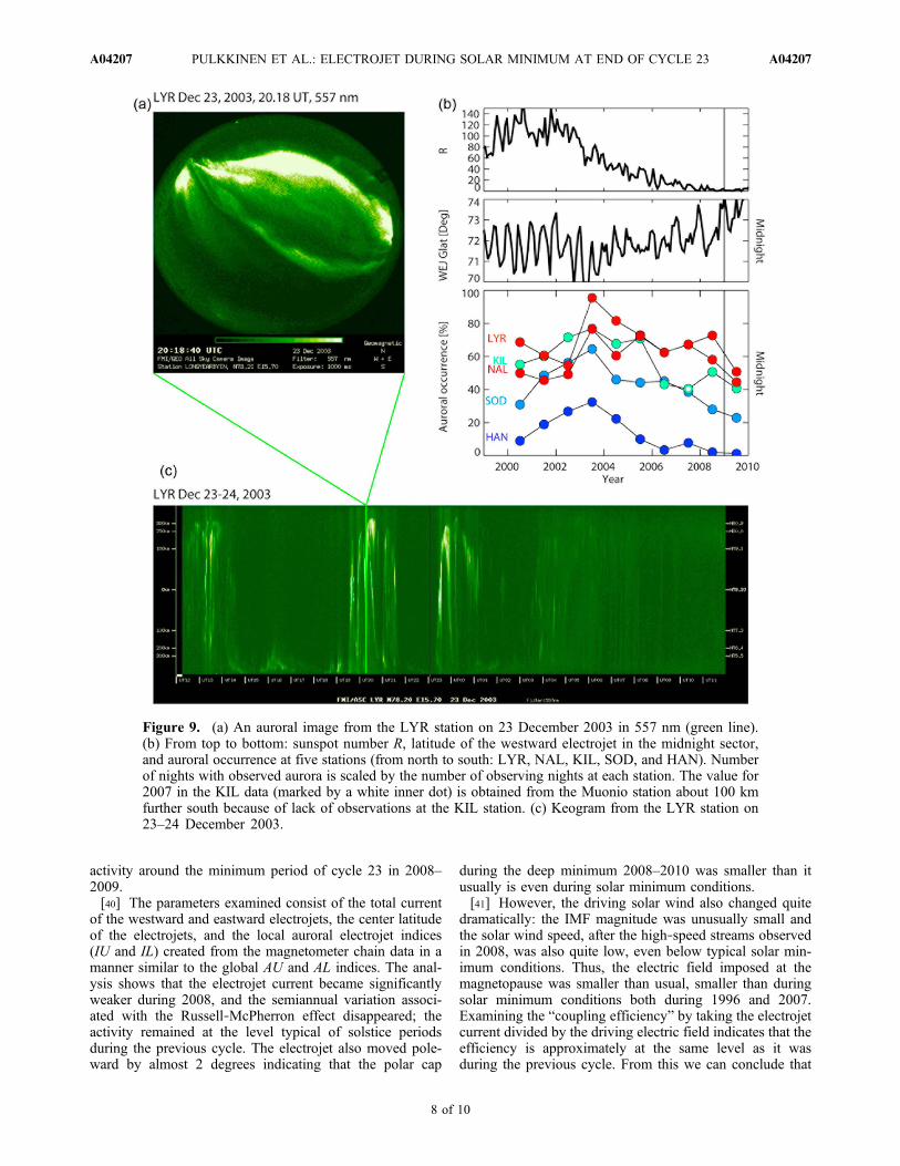
activity around the minimum period of cycle 23 in 2008–2009.[40] The parameters examined consist of the total current

of the westward and eastward electrojets, the center latitudeof the electrojets, and the local auroral electrojet indices(IU and IL) created from the magnetometer chain data in amanner similar to the global AU and AL indices. The anal-ysis shows that the electrojet current became significantlyweaker during 2008, and the semiannual variation associ-ated with the Russell‐McPherron effect disappeared; theactivity remained at the level typical of solstice periodsduring the previous cycle. The electrojet also moved pole-ward by almost 2 degrees indicating that the polar cap

during the deep minimum 2008–2010 was smaller than itusually is even during solar minimum conditions.[41] However, the driving solar wind also changed quite

dramatically: the IMF magnitude was unusually small andthe solar wind speed, after the high‐speed streams observedin 2008, was also quite low, even below typical solar min-imum conditions. Thus, the electric field imposed at themagnetopause was smaller than usual, smaller than duringsolar minimum conditions both during 1996 and 2007.Examining the “coupling efficiency” by taking the electrojetcurrent divided by the driving electric field indicates that theefficiency is approximately at the same level as it wasduring the previous cycle. From this we can conclude that

Figure 9. (a) An auroral image from the LYR station on 23 December 2003 in 557 nm (green line).(b) From top to bottom: sunspot number R, latitude of the westward electrojet in the midnight sector,and auroral occurrence at five stations (from north to south: LYR, NAL, KIL, SOD, and HAN). Numberof nights with observed aurora is scaled by the number of observing nights at each station. The value for2007 in the KIL data (marked by a white inner dot) is obtained from the Muonio station about 100 kmfurther south because of lack of observations at the KIL station. (c) Keogram from the LYR station on23–24 December 2003.

PULKKINEN ET AL.: ELECTROJET DURING SOLAR MINIMUM AT END OF CYCLE 23 A04207A04207

8 of 10

the solar wind‐ionosphere coupling processes were notaffected by the very quiet solar activity.[42] In this study, we employ the parallel electric field

EPAR = Esin(�/2) as the driver parameter. This parametergives the electric field along the large‐scale reconnectionline which forms across the dayside magnetopause. Thereconnection line lies in the equatorial plane during purelysouthward IMF, but becomes tilted for finite IMF BY values.This is why the EPAR is a better coupling function than theoften used EY based on only the southward BZ component ofthe IMF [Pulkkinen et al., 2010]. Other coupling functionshave also been employed such as the epsilon parameter � =(4p/m0)l0

2VB2sin4(�/2) [Akasofu, 1981], the Kan‐Lee electricfield EKL = VBTsin

2(�/2) [Kan and Lee, 1979], or the rateof magnetic flux opened at the magnetopause dF/dt =C[V 2BTsin

4(�/2)]2/3 [Newell et al., 2007], among others.

Here m0 is the vacuum permeability, l0 is an empiricalscaling parameter often set to 7 RE , and BT is the transversecomponent of the IMF perpendicular to the Sun‐Earth line,and C is a constant. Figure 10 compares results using dif-ferent drivers. It can be noted that all drivers have qualita-tively similar behavior over the solar cycle, and that theefficiencies computed using the different drivers vary inmagnitude depending on the scaling of the driver function,but have qualitatively similar behavior over the entireperiod. Thus, this shows that our results are robust and notdependent on the choice of a particular form of the couplingfunction.[43] Note that the choice of the driver function was made

based on the type of analysis: we do not have results thatwould conclusively prove one driver parameter superiorover another one. Each parameter has been derived for adifferent purpose, and thus have slightly different propertiestuned to give best results for the question addressed by theoriginal authors. Likewise, the absolute magnitude of theparameters depends on how they were scaled: the � param-eter was scaled to amount to energy equal to dissipated bythe ring current and by the ionosphere (including Jouleheating and auroral precipitation), the Newell parameteronly gives a functional form and is not scaled to any output.The electric field parameters only reference the externalsolar wind and IMF conditions with no scaling to dissi-pation in the magnetosphere‐ionosphere system. Thus, it isinevitable that each parameter has its optimum applicationsand that the numbers in absolute values are not directlycomparable.[44] We examined separately the local midnight sector,

which is most indicative of magnetospheric coupling pro-cesses. In this case, we only showed two years, 1996representing the minimum activity at the end of cycle 22,and 2009 representing the weak activity following theminimum at the end of 2008. Now there are clear indicationsof the electrojet being weaker and at further poleward lati-tude during 2009 than during 1996 for the same level ofsolar wind driving electric field. This would indicate that themagnetosphere was at a more quiet state during 2009 than itwas during 1996, thus feeding less of the energy enteringfrom the solar wind into the ionosphere. This is a naturalconsequence, e.g., of very low ring current intensity, whichwould increase the normal component of the plasma sheetmagnetic field and thus push activity further away from theinner magnetotail where it normally would reside [e.g.,Milan et al., 2009].[45] The quiet state of the magnetosphere is further

emphasized when the substorm events are analyzed indi-vidually. Using the data set created by Tanskanen [2009],we computed the monthly substorm amplitude and number.Both the amplitude of the substorms and the number ofsubstorms were quite low during 2009. Examining thecorrelations with the driving electric field it is clear that evenduring weak driving, there is a minimum number of sub-storms that occur, and that also the substorm size has aminimum value which is only weakly correlated with the(low level) of driving. The Dst index, which was very weakduring 2009, was also almost independent of the level ofsolar wind driving.[46] As the ring current in 2009 was very low, the mag-

netotail current sheet did not penetrate as close to the Earth

Figure 10. Comparison of different solar wind drivers.(top) Sunspot number R; (middle) solar wind driver functions� parameter [Akasofu, 1981] in GW, solar wind electric fieldEKL [Kan and Lee, 1979] (black) and EPAR [Pulkkinen et al.,2009] in mV/m, and magnetic flux opened at the magneto-pause dF/dt [Newell et al., 2007] (not scaled); and (bottom)efficiencies computed by dividing the westward electrojetcurrent by the driver function using hourly values.

PULKKINEN ET AL.: ELECTROJET DURING SOLAR MINIMUM AT END OF CYCLE 23 A04207A04207

9 of 10

than it does when the ring current is larger. This led to theinner magnetosphere field being more dipolar than it isunder more typical driving conditions. This causes themagnetic reconnection region and other associated substormdynamics to occur further away from the Earth than undermore average conditions. Under such conditions, midtailreconnection events may more often lead to large‐scale sub-storm activity, while their size may be limited by the abilityof the field‐aligned currents to couple to the ionosphere.[47] Long‐term auroral records show that indeed the

auroral distribution moves further poleward during low solaractivity periods. The data analysis involves millions ofimages of which separation of cloudy images from thosewith real auroras is challenging [Syrjäsuo et al., 2000], andthus this data set is quite unique extending over a completesolar cycle. All data sets used here, the electrojet database, thesubstorm database, and the auroral observations are consis-tent with each other, lending support to the conclusions.

8. Conclusions

[48] We demonstrate using auroral electrojet observations,substorm statistics, and auroral image analysis that theefficiency of the solar wind energy input to the drivenionospheric electrojets was no different during the veryquiet solar activity period 2008–2009 than during othertimes. On the other hand, we conclude that the very quietstate of the magnetosphere as demonstrated by the Dstvalues close to zero cause the magnetosphere‐ionospherecoupling to be slightly different: The substorm numberstayed at a higher level than expected based on the driverintensity (EPAR). Overall, this leads to slightly weakerelectrojet at further poleward latitudes in the midnightsector.

[49] Acknowledgments. We thank the NGDC for the solar data andthe NSSDC for compiling the OMNI database of long‐term solar windobservations. We thank the institutes who maintain the IMAGE Magne-tometer Array. The work of E.T. was supported by the Academy of Finlandgrants 108518 and 128632. Tero Raita at the Sodankylä GeophysicalObservatory (University of Oulu) and Stefano Massetti at IFSI‐INAF(Rome, Italy) are acknowledged for the maintenance of the Sodankyläand Ny‐Ålesund auroral cameras.[50] Robert Lysak thanks the reviewers for their assistance in evaluat-

ing this paper.

ReferencesAkasofu, S.‐I. (1981), Energy coupling between the solar wind and themagnetosphere, Space Sci. Rev., 28, 121–190.

Amm, O., and A. Viljanen (1999), Ionospheric disturbance magnetic fieldcontinuation from the ground to the ionosphere using spherical elemen-tary current systems, Earth Planets Space, 51, 431–440.

Baker, D. N., T. I. Pulkkinen, V. Angelopoulos, W. Baumjohann, and R. L.McPherron (1996), The neutral line model of substorms: Past results andpresent view, J. Geophys. Res., 101, 12,975–13,010.

Gibson, S. E., J. U. Kozyra, G. de Toma, B. A. Emery, T. Onsager, andB. J. Thompson (2009), If the Sun is so quiet, why is the Earth ringing?:A comparison of two solar minimum intervals, J. Geophys. Res., 114,A09105, doi:10.1029/2009JA014342.

Häkkinen, L. V. T., T. I. Pulkkinen, R. J. Pirjola, H. Nevanlinna, E. I.Tanskanen, and N. E. Turner (2003), Seasonal and diurnal variation ofgeomagnetic activity: Revised Dst vs. external drivers, J. Geophys.Res., 108(A2), 1060, doi:10.1029/2002JA009428.

Kan, J. R., and L. C. Lee (1979), Energy coupling function and the solarwind‐magnetosphere dynamo, Geophys. Res. Lett., 6, 577–580.

Kauristie, K., T. I. Pulkkinen, R. J. Pellinen, and H. J. Opgenoorth (1996),What can we tell about the AE‐index from a single meridional magne-tometer chain?, Ann. Geophys., 14, 1177–1185.

Kirk, M. S., W. D. Pesnell, C. A. Young, and S. A. Hess Webber (2009),Automated detection of EUV polar coronal holes during solar cycle 23,Sol. Phys., 257, 99–112, doi:10.1007/s11207-009-9369-y.

Lee, C. O., J. G. Luhmann, D. Odstrcil, P. J. MacNeice, I. de Pater,P. Riley, and C. N. Arge (2009), The solar wind at 1 AU during thedeclining phase of solar cycle 23: Comparison of 3D numerical modelresults with observations, Sol. Phys., 254, 155–183, doi:10.1007/s11207-008-9280-y.

Liou, K., P. T. Newell, and C.‐I. Meng (2001), Seasonal effects on auroralparticle acceleration and precipitation, J. Geophys. Res., 106, 5531–5542.

Lyatsky, W., P. T. Newell, and A. Hamza (2001), Solar illumination ascause of the equinoctial preference for geomagnetic activity, Geophys.Res. Lett., 28, 2353–2356.

Milan, S. E., A. Grocott, C. Forsyth, S. M. Imber, P. D. Boakes, andB. Hubert (2009), A superposed epoch analysis of auroral evolution dur-ing substorm growth, onset and recovery: Open magnetic flux control ofsubstorm intensity, Ann. Geophys., 27, 659–668.

Nevanlinna, H., and T. I. Pulkkinen (1998), Solar cycle correlations ofsubstorm and auroral occurrence frequency, Geophys. Res. Lett., 25,3087–3090.

Nevanlinna, H., and T. I. Pulkkinen (2001), Auroral observations inFinland: Results from all‐sky cameras, 1973–1997, J. Geophys. Res.,106, 8109–8118.

Newell, P. T., T. Sotirelis, K. Liou, C.‐I. Meng, and F. J. Rich (2007), Anearly universal solar wind magnetosphere coupling function inferredfrom 10 magnetospheric state variables, J. Geophys. Res., 112,A01206, doi:10.1029/2006JA012015.

Newell, P. T., T. Sotirelis, and S. Wing (2010), Seasonal variations indiffuse, monoenergetic, and broadband aurora, J. Geophys. Res., 115,A03216, doi:10.1029/2009JA014805.

Partamies, N., M. Syrjäsuo, and E. Donovan (2007), Using colour in auro-ral imaging, Can. J. Phys., 85, 101–109.

Pulkkinen, A., et al. (2003), Ionospheric equivalent current distributionsdetermined with the method of spherical elementary current systems,J. Geophys. Res., 108(A2), 1053, doi:10.1029/2001JA005085.

Pulkkinen, T. I., M. Palmroth, N. Partamies, H. E. J. Koskinen, T. V.Laitinen, C. C. Goodrich, J. G. Lyon, and V. G. Merkin (2009), Magne-tospheric modes and solar wind energy coupling efficiency, J. Geophys.Res., 115, A03207, doi:10.1029/2009JA014737.

Pulkkinen, T. I., M. Palmroth, H. E. J. Koskinen, T. V. Laitinen, C. C.Goodrich, V. G. Merkin, and J. G. Lyon (2010), Magnetospheric modesand solar wind energy coupling efficiency, J. Geophys. Res., 115,A03207, doi:10.1029/2009JA014737.

Russell, C. T., and R. L. McPherron (1973), Semiannual variation of geo-magnetic activity, J. Geophys. Res., 78, 92–108.

Sangalli, L., N. Partamies, M. Syrjäsuo, C.‐F. Enell, K. Kauristie, andS. Mäkinen (2010), Performance study of the new EMCCD‐based all‐sky cameras for auroral imaging, Int. J. Remote Sens., in press.

Syrjäsuo, M. T., et al. (1998), Observations of substorm electrodynamicsusing the MIRACLE network, in Substorms‐4: International Conferenceon Substorms‐4, Lake Hamana, Japan, March 9–13, 1998, edited byS. Kokubun and Y. Kamide, Astrophys. and Space Sci. Libr., vol. 238,pp. 111–114, Terra Sci., Tokyo.

Syrjäsuo, M. T., K. Kauristie, and T. I. Pulkkinen (2000), Searching forAurora, paper presented at International Conference on Signal andImage Processing (SIP‐2000), Int. Assoc. of Sci. and Technol. for Dev.,Las Vegas, Nev.

Tanskanen, E. I. (2009), A comprehensive high‐throughput analysis of sub-storms observed by IMAGE magnetometer network: Years 1993–2003examined, J. Geophys. Res., 114, A05204, doi:10.1029/2008JA013682.

Tanskanen, E. I., T. I. Pulkkinen, and H. E. J. Koskinen (2002), Substormenergy budget near solar minimum and maximum: 1997 and 1999 com-pared, J. Geophys. Res., 107(A6), 1086, doi:10.1029/2001JA900153.

Weiss, N. O., and S. M. Tobias (2000), Physical causes of solar activity,Space Sci. Rev., 94, 99–112.

K. Kauristie, N. Partamies, E. I. Tanskanen, and A. Viljanen, FinnishMeteorological Institute, PO Box 503, FI‐00101 Helsinki, Finland.T. I. Pulkkinen, School of Electrical Engineering, Aalto University,

PO Box 13000, FI‐00076 Aalto, Finland. (tuija.i.pulkkinen@aalto.fi)

PULKKINEN ET AL.: ELECTROJET DURING SOLAR MINIMUM AT END OF CYCLE 23 A04207A04207

10 of 10