author's personal copy - university of birmingham

This article appeared in a journal published by Elsevier. The attachedcopy is furnished to the author for internal non-commercial researchand education use, including for instruction at the authors institution

and sharing with colleagues.

Other uses, including reproduction and distribution, or selling orlicensing copies, or posting to personal, institutional or third party

websites are prohibited.

In most cases authors are permitted to post their version of thearticle (e.g. in Word or Tex form) to their personal website orinstitutional repository. Authors requiring further information

regarding Elsevier’s archiving and manuscript policies areencouraged to visit:

http://www.elsevier.com/authorsrights

http://www.elsevier.com/authorsrights

Author's personal copy

Original research article

On numerical uncertainty in evaluation of pest population size

N.L. Embleton *, N.B. Petrovskaya

School of Mathematics, University of Birmingham, Birmingham B15 2TT, UK

1. Introduction

Pest insects pose a serious problem to farmers as they can causesignificant damage to crops. In recent decades careful monitoringof pest insects became a common agricultural procedure wheremonitoring techniques are being improved and new, moreadvanced methods of monitoring are being designed (Foster andHarris, 1997; Chapman et al., 2002; Mei et al., 2012). Consequently,the problem of pest population size evaluation is an essential partof the pest monitoring program. This problem received a lot ofattention in the agricultural and ecological communities (Burn,1987; Metcalf, 1982), as an estimate of the pest population size inan agricultural field is required to decide whether or not it isnecessary to implement a control action (Ester and Rozen, 2005;Stern, 1973).

After an estimate of the pest population size has been obtained,the decision about any control action, often in the form ofpesticides, is then made based on the relation of the estimated pestabundance to some ‘critical density’ (Binns et al., 2000) or ‘actionthreshold’ (Dent, 1991). In other words, the estimated pestabundance is compared to the limiting level of pests at whichintervening is deemed to be worth the effort or expense. Making acorrect decision is important as lack of action could lead to the loss

of valuable crops. It is also the case that a wrong decision couldcause the unnecessary use of pesticides. Since pesticides are costlyand can have detrimental effects on both the environment andhuman health, it is important to avoid their use when they are notneeded (Blair and Zahm, 1991; Jepson and Thacker, 1990).

However making a correct decision about a control actionremains a difficult and challenging problem. One aspect of thisproblem is uncertainty introduced by estimating the populationsize by a chosen evaluation technique rather than counting eachindividual pest insect in the field. Consider, for instance, thesimple case of a single action threshold. If the average number ofpests obtained from the evaluation procedure falls below theaction threshold then the recommendation is that no actionshould be taken, whereas if the indication is that the averagenumber of pests is greater than the action threshold then thedecision should be to intervene (Stern, 1973). Obviously thisdecision making technique only becomes reliable if we have areliable estimate that does not significantly differ from the truevalue of the pest population size. Hence the problem of accurateevaluation of the number of pest insects is pivotal in the decisionmaking procedure.

Usually, an estimate is obtained through collecting samples andtheir subsequent analysis. One common method to collect samplesof the pest insect species is to apply a trapping procedure, where anumber of traps are installed across the monitored area. The trapsare then emptied after a certain period of waiting, the insectspecies of interest is identified and the number of such insects ineach trap is counted.

Ecological Complexity 14 (2013) 117–131

A R T I C L E I N F O

Article history:

Received 5 July 2012

Received in revised form 26 November 2012

Accepted 29 November 2012

Available online 16 January 2013

Keywords:

Pest monitoring

Sparse data

Mean density

Single peak

A B S T R A C T

Obtaining reliable estimates of pest insect species abundance is an essential part of ecological

monitoring programs. It is often the case that data available for obtaining such estimates are sparse

which in turn makes achieving an accurate evaluation difficult. This is especially true for strongly

heterogeneous pest population density distributions. In our paper we discuss the accuracy of a mean

density estimate when a certain class of high aggregation density distributions is considered and a

standard statistical method is employed to handle sparse sampled data. It will be shown in the paper that

conventional conclusions about the accuracy of the pest population size evaluation do not work when

the data are sparse and a new approach is required. Namely, if the number of traps is small, an estimate of

the mean density becomes a random variable with an error of high magnitude and we have to compute

the probability of an accurate estimate rather than computing the estimate itself. We have obtained a

probability of an accurate estimate based on the assumption that only one trap falls within a sub-domain

where the pest population density is different from zero. The probability has been calculated for the one-

dimensional and the two-dimensional problem.

� 2012 Elsevier B.V. All rights reserved.

* Corresponding author. Tel.: þ44 121 4142918; fax: þ44 121 4143389.

E-mail addresses: [email protected] (N.L. Embleton),

[email protected] (N.B. Petrovskaya).

Contents lists available at SciVerse ScienceDirect

Ecological Complexity

jo ur n al ho mep ag e: www .e lsev ier . c om / lo cate /ec o co m

1476-945X/$ – see front matter � 2012 Elsevier B.V. All rights reserved.

http://dx.doi.org/10.1016/j.ecocom.2012.11.004


It is worth noting here that more technically sophisticatedmethods such as mark-recapture (Lincoln, 1930) are also used byecologists as they can provide a more accurate alternative to thetrapping procedure above. However, for the routine monitoring ofinsect species methods of marking are time consuming, labourintensive and often too expensive (Hagler and Jackson, 2001)making such methods less practical.

Insect counts obtained via the trapping process provide thevalues of the pest population density at the trap locations (Byerset al., 1989; Raworth and Choi, 2001). An estimation of the pestabundance in the entire field can then be calculated from theinformation provided by the trap counts by statistical analysis(Davis, 1994; Seber, 1982), although some alternative methodshave recently been developed (Petrovskaya and Petrovskii, 2010;Petrovskaya and Venturino, 2011; Petrovskaya et al., 2012). Theaccuracy of an estimate depends on the number N of traps installedin the field. In theory, the estimate must tend to the true pestpopulation size when the number of traps gets infinitely large. Inreality, the number of traps always remains finite and anapproximate value always differs from the true pest populationsize. Moreover, it is in the interest of farmers and practicalecologists alike to make the number of traps as small as possible, asa large number of traps can bring considerable damage to theagricultural product. A large number of traps can also have adisruptive effect on the behaviour of the monitored insects andhence can result in a biased estimate of the population size.Another argument that must be taken into account is that atrapping procedure can be costly and labour-consuming. Thereasons above impose significant restrictions on the number oftraps installed over an agricultural field. It has been mentioned bymany authors (e.g. see Blackshaw, 1983; Ferguson et al., 2003;Holland et al., 1999) that the number of traps installed in a typicalagricultural field that has a linear size of a few hundred metresrarely exceeds a few dozen.

Let us define the approximation error as a difference betweenthe true value and an estimated value of the pest population size.Given the restrictions in a routine monitoring procedure, animportant question is to understand how big the approximationerror can be if the sampled data are sparse (e.g. because thenumber of traps is small). This question has been the focus ofecological research for a long time (Dent, 1991; Vlug and Paul,1986; Ward et al., 1985) and reliable recommendations have beenprovided on the minimum number of traps required for getting anaccurate estimate of a particular pest insect species (Binns et al.,2000; Karandinos, 1976; Southwood and Henderson, 2000). Thoserecommendations, however, are based on the assumption that thepest insect population is spread over the monitored area with(almost) uniform density. While this assumption is true for manyspecies, there also exists many ecologically important caseswhere the pest density is aggregated (Barclay, 1992; Fergusonet al., 2003; Petrovskaya et al., 2012). To our best knowledge, thecases of highly aggregated density distributions are not wellstudied in the literature, when a problem of pest abundanceevaluation is considered. Hence in our paper we study animportant case of an aggregated density distribution wherebythe entire pest population is confined to a single sub-region(patch) within an agricultural field and the pest population is zerooutside that patch. The term highly aggregated used throughoutthe paper refers to this particular type of density distribution.Such a distribution does have ecological significance as itcorresponds to the beginning of the biological invasion (Shigesadaand Kawasaki, 1997). Let us also note that the results obtained fora single patch can readily be extended to multi-patch densitydistributions.

The accuracy of population size estimation in the case ofhighly aggregated density was considered in our recent work

(Petrovskaya and Embleton, 2013) where we have used amethod of numerical integration (Davis and Rabinowitz, 1975).The analysis there proved the existence of the threshold numberNthreshold of traps, where the desired accuracy of pest populationsize evaluation can be achieved for any N � Nthreshold. In the casethat the number N of traps is N < Nthreshold, the approximationerror becomes a random variable with a large magnitudebecause of the insufficient information about the sampled data.Consequently, we have to evaluate the probability p of achievingan approximation error smaller than a given tolerance ratherthan to evaluate the error itself (Petrovskaya et al., 2012;Petrovskaya and Embleton, 2013). An immediate consequenceof this result is that the sampling plan has to be revisited whenwe have to deal with high aggregation density distributions, asan estimate of the pest population size per se becomesunreliable.

In the present paper we extend our earlier results to the casewhen a statistical counterpart of the numerical integration methodis used to evaluate the pest population size for high aggregationdensity distributions. This statistical method is a space-implicitmethod based on computation of the arithmetic mean of thepopulation density, where the average density is then multipliedwith the area of a monitored field (Seber, 1982; Snedecor andCochran, 1980). A widespread requirement that allows one to use amethod of numerical integration is that the traps locations shouldbe equidistant (Davis and Rabinowitz, 1975). Meanwhile thestatistical approach does not specify trap locations and it impliesthat any distance between traps is admissible. Moreover, acommon recommendation is to install traps randomly in the fieldin order to avoid biasing (Bliss, 1941; Legg and Moon, 1994; Reisenand Lothrop, 1999; Silver, 2008). It will be shown in the paper that,while the above recommendation works well for uniform densitydistributions (Perry, 1989; Alexander et al., 2005), randominstallation of traps may not always be optimal when highlyaggregated density distributions are considered. We analyse thestatistical method for an extreme case when only one trap fallsinside the sub-domain of the non-zero density as a result ofrandom installation of traps and conclude that an equidistantdistribution of traps is better. Furthermore, it will be demonstratedin the paper that, if an equally spaced grid of traps cannot beprovided, then installation of a certain (relatively small) number oftraps will be the most beneficial from the accuracy viewpoint, asfurther increase in the number of traps will result in a less accurateestimate of the pest population size.

The paper is organised as follows. In Section 1 we discuss theproblem statement and consider a few illuminating examples. Itwill be shown that the approximation error depends on howstrongly heterogeneous a density distribution is across themonitored area. We then focus our attention on high aggregationdensity distributions in Section 2 where the problem is reduced tothe one-dimensional case. It will be shown in Section 2 that theapproximation error becomes a random variable if the number oftraps is small and we explain how to compute the probability ofaccurate evaluation of the pest abundance. The results of Section 2are illustrated by numerical examples in Section 3. We continueour study in Section 4 where the analysis is extended to the two-dimensional case. In Section 5 the results of our study are used tocompare a random distribution of traps to a grid of equidistanttraps. The conclusions and discussion of our results are provided inSection 6.

2. The problem statement: evaluation of the mean densitywhen the data are sparse

In this section we discuss the accuracy problem when only asmall number of traps are available in a pest population size

N.L. Embleton, N.B. Petrovskaya / Ecological Complexity 14 (2013) 117–131118


evaluation procedure. Let N traps be installed over an agriculturalfield. We shall assume that the number of insects caught in eachtrap is an accurate representation of the true population density inits catchment area. Whilst we are aware that this assumption is notentirely realistic, it is not within the scope of this paper to considerthe problem of noisy data. However, it is worth mentioning herethat the effectiveness of trapping has been the focus of muchresearch (Legg and Moon, 1994; Petrovskii et al., 2012) and, withregard to our own work, two approaches can be considered thatallow one to deal with inaccurate measurements of the pestpopulation density. The first approach consists in developing atheoretical and methodological framework that enables a directestimate of populations from trap counts. For instance, it has beenshown in work (Petrovskii et al., 2012) that a ‘mean-field’ diffusionmodel is capable of revealing the generic relationship between trapcatches and population density. The second approach is to take thenoise into account when the data obtained as a result of trappingare handled by a method of numerical integration (Cox, 2007).Meanwhile we emphasize again that in the present paper weconsider a number of insects in each trap as the true populationdensity.

A statistical method commonly used in the evaluation of pestabundance depends on the sample mean pest population density(Davis, 1994). The mean density M(N) is defined as

MðNÞ ¼ 1

N

XN

i¼1

ui; (1)

where ui is the pest population density at each trap location(Snedecor and Cochran, 1980). The sample mean value M(N) acts asan approximation to the true mean value E. An approximationSapprox to the actual pest population size S can then be found bymultiplying the sample mean by the area of the field A, that is

S � Sapprox ¼ AMðNÞ: (2)

The decision about any control action with regard to pestinsects is usually based on the assumption that the approximationSapprox is close to the true value S of the pest population size. Whilethis assumption is correct in many cases, there can be densitydistributions where the formulae (1) and (2) present poorapproximation of the true population size. Below we illustratethis statement by considering several density distributions overthe unit square. Since the area A = 1, we will focus our attention onthe estimate (1) where our aim is to demonstrate that the accuracyof approximation (1) depends strongly on the spatial heterogeneityof a density distribution.

Despite plenty of experimental data being available in the pestinsect monitoring problem, in our further discussion we will usethe data obtained as a result of computer simulation. This isbecause we need a sequence of values (1) obtained when weincrease the number of traps for each consequent computation of(1). Hence we take our data from an ecologically soundmathematical model of population dynamics in order to be ableto reconstruct the function M(N) for various N of our choice.Namely, we consider the spatially explicit predator-prey modelwith the Allee effect (Murray, 1989; Turchin, 2003). In thedimensionless form the system is as follows:

@uðx; y; tÞ@t

¼ d@2

u

@x2þ @2

u

@y2

!þ buðu � bÞð1 � uÞ � uv

1 þ Lu; (3)

@vðx; y; tÞ@t

¼ d@2v@x2þ @2v

@y2

!þ uv

1 þ Lu� mv; (4)

where u(x, y, t) and vðx; y; tÞ are the densities of prey and predator,respectively, at time t > 0 and position (x, y), d is the diffusion

coefficient, and the other parameters have evident meaning(Murray, 1989).

In order to obtain the population density distributions, thesystem ((3) and (4)) is solved numerically for a range ofparameters, where the function u(x, y, t) obtained as a result ofcomputation is considered as the density of the pest insect in theproblem. For the discussion of the numerical solution along withthe choice of the initial and boundary conditions we refer theinterested reader to our paper (Petrovskaya et al., 2012) wheresimilar computer simulations have been carried out.

Let us fix the time t as t ¼ t > 0 and consider a snapshotuðx; yÞ � uðx; y; tÞ of a temporal–spatial density distribution u(x, y,t). Numerical solution of (3) and (4) at any fixed time t provides uswith the discrete density distribution ui � u(ri), i = 1, . . ., N wheregrid nodes ri = (xi, yi) are the points where traps are located. Wethen use the formula (1) to compute the mean value of a discretefunction u(x, y) considered on a grid of N traps.

Since the solution u(x, y) is not available in closed form, we firstsolve the system ((3) and (4)) for a very big number of traps N = Nf,where Nf = NxNy and Nx = Ny = 210 + 1 is the number of trapsinstalled in the x and y-directions of a rectangular grid,respectively. The mean value E computed for N = Nf is consideredas the true mean density and the spatial density distribution u(x, y)obtained on a grid of Nf nodes at fixed time t is stored for furthercomputations. We then decrease the total number N of grid nodesand consider several approximations M(N) of the true mean E

obtained for smaller values of N. The formula (1) is used to obtainM(N) every time that we decrease N in our computations. Let usnote that we do not re-compute the density function u(ri), i = 1, . . .,N every time that a new number N is chosen. The values of u(x, y)are always taken from the ‘exact solution’ computed on a grid of Nf

nodes at time t, where we make a projection of the function u(ri),i = 1, . . ., Nf obtained on the fine grid to a coarse grid every time thatwe take a new, smaller number N of nodes. For instance, if weconsider the grid of Nf nodes and collect the data u(ri) at each 4thgrid node in the x-direction and in the y-direction alike, we obtainthe density distribution on a coarser grid where the total numberof nodes (traps) will be 16 times smaller in comparison with theoriginal fine grid. The details of this computational technique arediscussed in our previous work (Petrovskaya and Petrovskii, 2010).

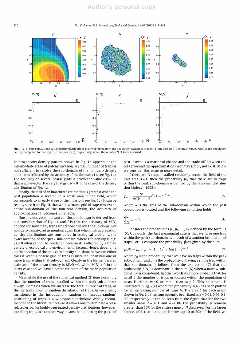
Several density distributions obtained as a result of numericallysolving (3) and (4) on a grid of Nf nodes are shown in Fig. 1a–c. Thedensity functions u(x, y) shown in Fig. 1a–c can be generated for awide variety of the initial and boundary conditions; seePetrovskaya et al. (2012). For each density function u(x, y)presented in Fig. 1a–c we show the true value E and the curveM(N) in Fig. 1d–f respectively, where N is the number of nodes ineach direction of a rectangular grid and the total number of nodesN ¼ N

2. For the sake of convenience both M(N) and E are scaled by

the value of the true density, so that E = 1 in the figure.It can be concluded from Fig. 1 that the accuracy of the

estimation depends on how the pest insects are dispersed acrossthe agricultural field. The density distribution u(x, y) shown inFig. 1a is a snapshot of the propagation of a continuous front. Thisdensity distribution is not strongly heterogeneous and the formula(1) gives us a very good estimate of the true mean density E even ifthe number of nodes is small (see Fig. 1d). Let us define the relativeapproximation error as err = (|E � M(N)|)/E, then the error iserr � 0.2 even on a very coarse grid with N = 9 (the number oftraps in each direction is N ¼ 3).

The conclusion about accuracy on coarse grids is, however,different when the density distributions shown in Fig. 1b–c areconsidered. Both of these distributions present an ecologicallyimportant case of ‘‘patchy invasion’’ when the whole population isoriginally localised in a small sub-domain somewhere in themonitored area (Petrovskii et al., 2002, 2005). A strongly

N.L. Embleton, N.B. Petrovskaya / Ecological Complexity 14 (2013) 117–131 119


heterogeneous density pattern shown in Fig. 1b appears at theintermediate stage of patchy invasion. A small number of traps isnot sufficient to resolve the sub-domain of the non-zero densityand that is reflected by the accuracy of the formula (1) (see Fig. 1e).The accuracy on several coarse grids is below the value err � 0.2that is achieved on the very first grid N = 9 in the case of the densitydistribution of Fig. 1a.

Finally, the risk of an inaccurate estimation is greatest when thepest population is located in a small area of the field, whichcorresponds to an early stage of the invasion (see Fig. 1c). It can bereadily seen from Fig. 1f, that when a coarse grid of traps misses theentire sub-domain of the non-zero density, the accuracy ofapproximation (1) becomes unreliable.

One obvious yet important conclusion that can be derived fromour consideration of Fig. 1c and f is that the accuracy of M(N)depends on how many traps are stationed inside the sub-domain ofnon-zero density. Let us mention again that when high aggregationdensity distributions are considered in ecological problems, theexact location of the ‘peak sub-domain’ where the density is u(x,y) 6¼ 0 often cannot be predicted because it is affected by a broadvariety of ecological and environmental factors. Hence, dependingon the location of the non-zero density sub-domain, we can eithermiss it when a coarse grid of traps is installed, or install one ormore traps within that sub-domain. Clearly in the former case anestimate of the mean density is M(N) = 0, while M(N) > 0 in thelatter case and we have a better estimate of the mean populationdensity.

Meanwhile the use of the statistical method (2) does not implythat the number of traps installed within the peak sub-domainalways increases when we increase the total number of traps, asthe method allows for random distribution of traps. As we alreadymentioned in the introduction, random (or pseudo-random)positioning of traps is a widespread technique widely recom-mended in the literature because it allows one to eliminate a bias-related error. For highly aggregated density distributions, however,installing traps in a random way means that detecting the patch of

pest insects is a matter of chance and the trade-off between thebias error and the approximation error may simply not exist. Belowwe consider this issue in more detail.

If there are N traps installed randomly across the field of theunit area A = 1, then the probability pm that there are m trapswithin the peak sub-domain is defined by the binomial distribu-tion (Spiegel, 1992):

pm ¼N!

m!ðN � mÞ! dmð1 � dÞN�m; (5)

where d is the area of the sub-domain within which the pestpopulation is located and the following condition holds:

XN

m¼0

pm ¼ 1: (6)

Consider the probabilities p0, p1, . . ., pN defined by the formula(5). Obviously, the first meaningful case is that we have one trapwithin the peak sub-domain as a result of a random installation oftraps. Let us compute the probability pðNÞ given by the sum

pðNÞ ¼ p0 þ p1 ¼ ð1 � dÞN þ Ndð1 � dÞN�1; (7)

where p0 is the probability that we have no traps within the peaksub-domain, and p1 is the probability of having a single trap withinthat sub-domain. It follows from the expression (7) that theprobability pðNÞ is dominant in the sum (6) when a narrow sub-domain d is considered. In other words it is more probable that, forsmall d the number of traps m located within the population ofpests is either m = 0 or m = 1 than m � 2. This statement isillustrated in Fig. 2(a) where the probability pðNÞ has been plottedfor an increasing number of traps N. The area d for each graphshown in Fig. 2(a) has consequently been fixed as d = 0.01, 0.06, 0.1,0.2, respectively. It can be seen from the figure that for the twosmaller areas d = 0.01 and d = 0.06 the probability p remainsgreater than 50% for the entire range of N displayed. For the largerchoices of d, that is the patch takes up 10 or 20% of the field, we

0 50 10 0 15 0 200 25 00

0.2

0.4

0.6

0.8

1

M(N)

E

N

d

~0 50 10 0 15 0 20 0 25 0

0

0.2

0.4

0.6

0.8

1

M(N)

E

N

e

~0 50 10 0 15 0 20 0 25 0

0

0.2

0.4

0.6

0.8

1

M(N)

E

N

f

~

X

Y

0 0. 2 0. 4 0. 6 0. 8 10

0.2

0.4

0.6

0.8

0.85

0.75

0.65

0.55

0.45

0.35

0.25

0.15

u(x, y)a

X

Y

0 0. 2 0. 4 0. 6 0. 8 10

0.2

0.4

0.6

0.8

0.85

0.75

0.65

0.55

0.45

0.35

0.25

0.15

0.05

u(x, y)b

X

Y

0 0. 2 0. 4 0. 6 0. 8 10

0.2

0.4

0.6

0.8

0.85

0.75

0.65

0.55

0.45

0.35

0.25

0.15

0.05

u(x, y)c

Fig. 1. (a–c) Pest population spatial density distributions u(x, y) obtained from the population dynamics model ((3) and (4)). (d–f) The mean values M(N) of the population

density computed for density distributions (a–c), respectively, when the number N of traps is varied.



have pðNÞ > 0:5 for N � 16 and N � 8 respectively. In Fig. 2(b) asimilar graph has been plotted, except this time the area of thepatch of pests is varied for fixed values of the total number of trapsN. In each case there is a range of sub-domain areas d for which thecondition pðNÞ > 0:5 is satisfied. Thus the probability pðNÞ isdominant when the patch is small in comparison to the area of thefield, a situation which corresponds to an early stage of biologicalinvasion. The observations made above will be further discussed inSection 6.

The conclusion that we make here is that the bias problem is notvery important when a single peak distribution is considered, asthe most likely scenario is that we lose either all or all but one trapsoutside the peak sub-domain. Hence, the question we would like toinvestigate is whether a random trap distribution is still betterthan a grid of equidistant traps for highly aggregated density ofpest insects. Clearly, a complete answer to this question wouldrequire investigation of all cases described by the formula (5), thatis one trap within the peak sub-domain, two traps within the peaksub-domain, etc. However, in the present paper we restrict ourdiscussion to the case of a single trap placed within the peak sub-domain even when the total number of traps is big. Despite thiscase not giving us a complete answer to the question of accurateestimation of the pest abundance, its study will allow us to identifyand resolve several very important issues related to handlingstrongly localised density distributions. In particular, it will berevealed that a standard approach in the evaluation of the pestpopulation size should be revisited when a highly aggregateddensity distribution is considered. In the next section we will showthat the approximation error should be handled as a randomvariable and will compute the probability of obtaining an accurateestimate of the pest population size.

3. The analysis of a high aggregation density distributions: 1Dcase

3.1. Probability of obtaining an accurate estimate of the true mean

population density

The spatial heterogeneity of a one-peak distribution u(x) can bethought of as being constructed of two components – a peak regionand a tail region. Clearly the peak is a dominant feature of thedensity u(x) and it provides the main contribution to the meandensity M(N). Hence for the sake of our further discussion weformulate a simplified version of the distribution u(x). In the peakregion we consider u(x) as a quadratic function of the width d.Elsewhere we set the population density to be zero, therefore the

tail region is essentially ‘cut off’. We then have

uðxÞ � gðxÞ ¼ B � Aðx � x�Þ2; x 2 ½xI; xII�;0; otherwise;

�(8)

where x* is the location of the maximum of the peak, A = � (1/2)(d2u(x*)/dx2), B = u(x*). The peak width is d ¼ 2

ffiffiffiffiffiffiffiffiffiB=A

pand the

roots are xI = x* � d/2, xII = x* + d/2.The above approximation of an arbitrary peak function u(x) by a

quadratic function g(x) is very convenient, as it allows one to derivesome important theoretical results about the accuracy of theformula (1). At the same time, the question of reliability ariseswhen we replace our original density distribution u(x) with asimpler function g(x) as such a replacement introduces the errorthat depends on the peak width d. However, the numerical studymade in Petrovskaya and Embleton (2013) demonstrated that ourconclusions about the quadratic approximation can be extended tothe case when arbitrary peak functions are considered. Hence weconsider the approximation as being reliable and use it in ourfurther analysis.

Let N be the number of traps distributed over the domain andthe density values u(xi) � ui be known at locations xi. As we alreadymentioned in the previous section we intend to consider thelimiting case of one trap installed in the domain [xI, xII], where wehave non-zero density u(x). In other words, if the traps numerationis i = 1, 2, . . ., N, then we have ui0

6¼ 0 for fixed i = i0 and ui = 0 for anyi 6¼ i0. Let us re-define the index i0 as i0 = 0 for the sake ofconvenience. The trap location xi0

� x0, where the densityui0� u0 6¼ 0, is defined as

x0 ¼ x� þ gd2;

where the parameter g 2 [0, 1] as we only consider the right half ofthe peak sub-domain, because of the obvious symmetry of the peak(see Fig. 3b).

The density u0 is computed as

u0 � gðx0Þ ¼ B � Aðx0 � x�Þ2 ¼ Bð1 � g2Þ; g 2 ½0; 1�; (9)

where we take into account that d=2 ¼ffiffiffiffiffiffiffiffiffiB=A

p.

Let now E be the true mean density and we require theapproximation error to be small when E is approximated by M(N):

err ¼ jE � MðNÞjE

< t; (10)

0 2 4 6 8 10 12 14 16 18 200

0.1

0.2

0.3

0.4

0.5

0.6

0.7

0.8

0.9

1

N

p(N

)

a

δ=0.01δ=0.06δ=0.1δ=0.2

0 0.2 0.4 0.6 0.8 10

0.1

0.2

0.3

0.4

0.5

0.6

0.7

0.8

0.9

1

δ

p(δ

)

b N=5N=10N=15

Fig. 2. The probability pðNÞ given by the formula (7). (a) The value of the total number of traps N varies and the area of the peak sub-domain d is fixed. (b) N is fixed and d varies.



where t is a prescribed tolerance, 0 < t < 1. Hence the mean valueM(N) computed when we use N traps should be within the range

ð1 � tÞE � MðNÞ � ð1 þ tÞE: (11)

We have already mentioned in the previous section that inecological applications the exact location of the peak sub-domaincannot be predicted for a high aggregation density distribution. Wenow make an assumption that is crucial for our further discussion.Since the location of the sub-domain [xI, xII] is not known, with anylocation as likely to occur as another, the location x* of the peakmaximum can be considered to be a uniformly distributed randomvariable. Under the requirement that only one trap lies in thedomain [xI, xII] the assumption about uniformly random location ofthe peak sub-domain can be re-formulated in terms of the locationof the point x0. Namely, we fix the point x* and then consider g 2 [0,1] as a uniformly distributed random variable in order torandomise the location of x0.

We now solve the inequalities (11) in order to see whether anylocation x0 of a trap within the peak sub-domain can provide thedesirable accuracy (11). The mean density is

MðNÞ ¼ u0

N¼ Bð1 � g2Þ

N; (12)

where (9) has been taken into account. Meanwhile, for a quadraticdensity distribution g(x) the true mean density E is given by

E ¼Z 1

0gðxÞdx ¼ 2

3Bd: (13)

Substituting M(N) and E in (11) we arrive at

ð1 � tÞBd � Bð1 � gÞ2

N� ð1 þ tÞBd; (14)

where d ¼ ð2=3Þd.Consider the inequality

Bð1 � gÞ2

N� ð1 þ tÞBd: (15)

We have

1 � g2 � ð1 þ tÞNd ) g � g I ¼ffiffiffiffiffiffiffiffiffiffiffiffiffiffiffiffiffiffiffiffiffiffiffiffiffiffiffiffiffiffi1 � ð1 þ tÞNd

q; (16)

where we have to choose a positive root, as g 2 [0, 1]. It followsfrom the solution of (16) that the number N of traps should be

restricted as

N � N� ¼ 1

dð1 þ tÞ: (17)

If the restriction (17) breaks, then the inequality (15) holds for anyg 2 [0, 1].

Let us now solve

Bð1 � g2ÞN

� ð1 � tÞBd: (18)

Similar computation results in

1 � g2� ð1 � tÞNd ) g � g II ¼ffiffiffiffiffiffiffiffiffiffiffiffiffiffiffiffiffiffiffiffiffiffiffiffiffiffiffiffiffiffi1 � ð1 � tÞNd

q; (19)

where the number of traps is restricted as

N � N�� ¼ 1

dð1 � tÞ: (20)

If the restriction (20) does not hold then the accuracy (11)is never achieved. In other words, if we have a big numberN > N** of traps, but they are randomly distributed over theentire area [0, 1], so that only one trap is positioned within thepeak sub-domain, then the accuracy of the mean densityevaluation will always be poor, as M(N) will not be withinthe range (11).

Let us note that the number N* < N** for any peak width d andtolerance t. Hence we have to consider the following cases

Case 1: N � N* .For any number of traps that is smaller than N* the admissible range oftrap locations x0 where we can guarantee prescribed accuracy (11) isgiven by gI � g � gII. In other words, we require that x0I

� x0 � x0II,

where x0I¼ x� þ g Iðd=2Þ and x0II

¼ x� þ g IIðd=2Þ.The same result holds when we consider a trap location at the

left-hand side of the peak, x0 = x* + g(d/2), where g 2 [�1, 0]. Wetherefore have two subintervals [� gII, � gI] and [gI, gII] where thetrap location within each of those subintervals will give us theaccuracy required by (11). As the length of the entire interval isg 2 [�1, 1] and a trap is randomly placed at any point of the peaksub-domain, then the probability p(N) of obtaining a value M(N)

x0

g(x)

x*x

b

0 0. 2 0. 4 0. 6 0. 8 1 1

0.2

0.4

0.6

0.8

1

au(x)

x0

Fig. 3. (a) An example of high aggregation density distribution in a 1D ecological system. (b) Approximation of the one peak density distribution by a quadratic function. One

trap is installed at the location x0 within the peak sub-domain.



that meets the condition (11) is given by

pðNÞ ¼ 2ðg II � g IÞgmax � gmin

; (21)

where gmin = �1, gmax = 1 and we multiply the range gII � gI by 2 aswe now consider the left-hand side and the right-hand side of thepeak. Substituting gI and gII from (16) and (19) respectively inEq. (21) we arrive at

pIðNÞ ¼ffiffiffiffiffiffiffiffiffiffiffiffiffiffiffiffiffiffiffiffiffiffiffiffiffiffiffiffiffiffi1 � ð1 � tÞNd

q�

ffiffiffiffiffiffiffiffiffiffiffiffiffiffiffiffiffiffiffiffiffiffiffiffiffiffiffiffiffiffi1 � ð1 þ tÞNd

q: (22)

The probability pI(N) for N < N* is shown as branch I of the graphin Fig. 4a. It can be seen from the graph as well as from theanalytical expression (22) obtained for the probability p(N) thatthe maximum value pmax ¼ pmaxðtÞ ¼

ffiffiffiffiffiffiffiffiffiffiffiffiffiffiffiffiffiffiffiffiffiffiffiffiffiffiffiffiffiffiffiffiffiffiffiffiffiffiffiffiffiffiffiffiffi1 � ðð1 � tÞ=ð1 þ tÞÞ

pof

the probability p(N) is achieved when N = N*. It is important to notehere that the maximum probability is always pmax < 1. At the sametime the probability pmax(t) predictably grows when we make thetolerance t bigger, that is pmax! 1 as t ! 1.

Case 2: N* < N � N** .For any number of traps N > N* the inequality (15) always holds.Hence we only have the restriction (20) and the admissible range of gbecomes g 2 [0, gII]. The probability of obtaining an accurate estimate(11) is given by

pIIðNÞ ¼ffiffiffiffiffiffiffiffiffiffiffiffiffiffiffiffiffiffiffiffiffiffiffiffiffiffiffiffiffiffi1 � ð1 � tÞNd

q: (23)

The probability pII(N) defined for the number of trapsN* < N � N** is shown as curve II in Fig. 4a.

Case 3: N > N** .In the case that N is sufficiently big, the probability of the event thatthe error is within the range (11) is pIII(N) = 0 as we cannot meet thecondition (18) (see branch III in Fig. 4a).

Let us note again that the results above are entirely based on theassumption that only one trap belongs to the peak sub-domain.However, we emphasize again that if a random distribution oftraps over the domain is applied, then we cannot guarantee thatmore than one trap will be located in the peak sub-domain evenwhen the total number N of traps is big (see discussion inSection 2). The branches II and III of the curve p(N) in Fig. 4a willexist as long as we have a single trap within the peak sub-domain,no matter how big the total number N of traps is. Hence if we wantto keep a random distribution of traps, our recommendation wouldbe to restrict the number of traps as N � N* as this number of traps

would give us the biggest chance to get an accurate estimate of themean density M(N).

4. Numerical results

In this section the probability p(N) will be obtained in severaltest cases by direct computation and compared with a theoreticalcurve obtained for a quadratic function (8). The first test case is toconfirm that our theoretical results derived for a quadratic functionare correct. Let us fix the peak width d, the tolerance t and the peaklocation x*. We then consider the location x0 of a trap as a randomvariable that is uniformly distributed over the interval [x*, x* + d/2].In our computations we provide nr = 100,000 realisations of therandom variable x0 for the fixed number N of traps, compute M(N)and check the condition (11) for each realisation of x0. Theprobability p(N)comput of the accurate evaluation (11) of the meandensity is then computed as

pðNÞcomput ¼nr

nr; (24)

where nr is the number of realisations for which the condition (11)holds. We then increase the number of traps by one and repeatcomputation (24) for N + 1 traps. We stop increasing the number N,when the number NL of traps becomes so big that the condition(20) breaks and we have p(NL) = 0.

The probability p(N)comput of the accurate evaluation of themean density is shown in Fig. 4b for the peak width d = 0.06 andthe tolerance t = 0.25. We start from N1 = 1 trap and thenincrease the number of traps until NL = 40. It can be seen fromthe figure that all values of the probability p(N)comput, N = 1, . . .,40, computed by direct evaluation (24) belong to the theoreticalcurve p(N).

The probability (22) and (23) is further illustrated for aquadratic function (8) in Fig. 5. Again, we assume that only onetrap is located within the peak sub-domain and the location of thattrap is random with respect to the position of the peak maximum.We make 100 random realisations nr of the trap location x0 andcompute the error (10) for each realisation when the number oftraps is fixed as N = 10. The integration error (10) computed for thefunction (8) is shown in Fig. 5a. The theoretical value of theprobability p(N) is p(N) = 0.12 when N = 10. This is well illustratedby the results shown in Fig. 5a where approximately 10% of theerror values belong to the range (11). Clearly, the value p � 0.1must tend to the theoretical probability p(N) = 0.12 when weincrease the number of realisations nr (cf. Fig. 4b). Consider nowN = N*, where the optimal number N* of traps is defined from (17)as N* = 20 for the peak width d = 0.06 and the tolerance t = 0.25.

N

pmax

a

N**N*

p(N)

III

III0 10 20 30 400

0.1

0.2

0.3

0.4

0.5

0.6

0.7computational results

theoretical curve

N

p(N) b

Fig. 4. The probability of obtaining an accurate estimate M(N) of the true mean density E in the case when a single trap is installed within a peak subdomain formed by a

quadratic function (8). (a) The theoretical curve. (b) Comparison of the theoretical curve and computational results. The probability is computed for the peak width d = 0.06

and the tolerance t = 0.25.



The probability of an accurate estimate is p(N*) = 0.66 and thisresult is confirmed by the error distribution shown in Fig. 5b wheremost of the error values (every 2 out of 3) lie within the requiredrange.

Let us now consider several standard test cases where highaggregation density distributions are different from the quadraticfunction (8). The test cases below are taken from the work(Petrovskaya and Embleton, 2013) where they have beeninvestigated for the midpoint integration rule. Our first test caseis to consider the cubic function

uðxÞ ¼Aðx � x� þ ðd=3ÞÞðx � x� � ð2d=3ÞÞ2; x 2 ½x� � d=3; x� þ 2d=3�;0; otherwise;

8<:

(25)

where the peak width is d = 0.06 and A = 30,000. We apply the samecomputational procedure (24) as for the quadratic functiondiscussed above to obtain the probability p(N)comput for variousN. The probability graph for the function (25) is shown in Fig. 6a.Obviously, the probability graph obtained for a cubic functioncannot coincide with the theoretical curve (22) and (23) (a dashedline in Fig. 6a). In particular, the critical number N* = 24 is nowdifferent from the theoretical value N* = 20 computed from (17) fort = 0.25 and d = 0.06. Nevertheless, it can be seen from the figurethat the theoretical curve obtained for a quadratic function is agood approximation of the probability p(N) computed for a cubicfunction (25).

A quartic function is defined as

uðxÞ ¼A

d2

� �4

� ðx � x�Þ4 !

; x 2 ½x� � d2; x� þ d

2�;

0; otherwise;

8>>><>>>:

(26)

where A = 1,200,000 and the peak width is again taken as d = 0.06.The probability graph for the function (26) is shown in Fig. 6b. Itcan be seen from the figure that the graph has a similar shape to thetheoretical graph for the quadratic function, but the criticalnumber N* = 17 is again different from the number N* = 20obtained from the analysis of a quadratic distribution.

Finally, we consider a normal distribution

uðxÞ ¼ 1

sffiffiffiffiffiffiffi2pp exp �1

2

ðx � x�Þ2

s2

!; (27)

that gives us an example of a peak function that is different fromzero everywhere in the domain x 2 [0, 1]. The peak width is definedby the parameter s as d = 6s and we again consider d = 0.06. Theprobability graph computed from (24) for the function (27) isshown in Fig. 6c. It can be seen from the figure that the criticalnumber N* = 33 strongly differs from the number of traps obtainedfor a quadratic function with the same peak width. However, theshape of the graph is still similar to the theoretical curve (a dashedline in the figure) and the critical value N* of traps provides themaximum probability p(N*). The presence of the critical value N* in

20 40 60 80 100

0.2

0.4

0.6

0.8

1

1.2

1.4

nr

aerr

τ

20 40 60 80 100

0.2

0.4

0.6

0.8

1

1.2

1.4

nr

berr

τ

Fig. 5. Computation of the error (10) for a random peak location. The peak is given by a quadratic function (8) of width d = 0.06. The tolerance in the formula (10) is t = 0.25. A

location of the peak is randomly generated 100 times and the error value is computed for each realisation nr = 1, 2, . . ., 100 of the peak location. (a) The number of traps is

N = 10. The probability of getting the error err < t is low and most of the error values are beyond the required range. (b) The number of traps is N = N* = 20. The probability of

getting an accurate answer err < t achieves its maximum when N = N* and most of the error values are within the required range.

0 10 20 30 400

0.1

0.2

0.3

0.4

0.5

0.6

0.7computational resultstheoretical curve for a quadratic function

N

p( N)

N*

a

0 10 20 30 40 50 600

0.1

0.2

0.3

0.4

0.5

0.6


N

p( N)

N*

c

0 10 20 30 400

0.1

0.2

0.3

0.4

0.5

0.6

0.7


N

p( N)

N*

b

Fig. 6. Numerical test cases. The probability (24) (solid line) of an accurate answer (11) computed for (a) cubic function (25); (b) quartic function (26) and (c) normal

distribution (27). For the functions (a)–(c) the peak width is chosen as d = 0.06. For each function (a)–(c) the probability (24) is compared with the theoretical curve obtained

for a quadratic function (dashed line).



each graph in Fig. 6 remains the most essential feature of ouranalysis.

4.1. Ecological test cases

In this subsection we verify our estimate (17) of the criticalnumber N* of traps when ecologically meaningful peak functionsare considered. In our consideration of ecological test cases we usethe pest density distributions u(x) generated from the one-dimensional counterpart of the system (3) and (4). The parametersof the one-dimensional system of equations as well as the initialand boundary conditions required for its numerical solution arediscussed in detail in the paper (Petrovskaya and Petrovskii, 2010).The function u(x, t) considered at fixed time t gives us a one-dimensional spatial density distribution uðx; tÞ � uðxÞ of the pestinsect over the unit interval x 2 [0, 1].

Similarly to the 2D case the properties of the spatial distributionu(x) considered at a given time t are determined by the diffusion d.Namely, the density distribution can evolve into the one-peakspatial pattern if the diffusion is d 1. The examples of one-peakdensity distributions are shown in Fig. 7, where the functions u(x)have been obtained from the numerical solution for the diffusioncoefficient d = 10�4 and d = 10�5 respectively. The diffusioncoefficient d is a controlling parameter in the problem and ithas been discussed in Petrovskii et al. (2003), Malchow et al. (2008)that the peak width d depends on the value of d. A simple estimate

of the function d(d) can be written as

d ¼ vffiffiffidp

; (28)

see Petrovskii et al. (2003), where it has been argued that thecoefficient v in the expression (28) is relatively robust to changesin the parameter values, and can typically be considered as v � 25.Hence the critical number of traps can be evaluated as

N� ¼ 1

dð1 þ tÞ� Cffiffiffi

dp ; (29)

where the coefficient C(t) = 3/(2v(1 + t)).Consider the density distribution u1(x) shown in Fig. 7a. Since

the diffusion coefficient is d = 10�4, the estimate (29) gives us thenumber N* � 5 for the tolerance t = 0.25. The probability graphobtained by direct computation is shown in Fig. 7b, where thenumber N* = 7 taken from the graph is in good agreement with thetheoretical estimate.

Let us now evaluate the number N* in the case that we have thedensity distribution u2(x) shown in Fig. 7c. For the diffusioncoefficient d = 10�5 we have N* � 16. The direct computation givesus N* = 23 which is greater than the theoretical value of N* obtainedfor a quadratic function. However, the results obtained for aquadratic function are still true for an ecologically meaningfuldensity distribution. Namely, if traps are randomly installed overthe monitored area and we cannot guarantee that more than one

0 0. 2 0. 4 0. 6 0. 8 1

0.2

0.4

0.6

0.8

1

au1(x)

x

0 0. 2 0. 4 0. 6 0. 8 10

0.1

0.2

0.3

0.4

0.5

0.6

u2(x)

x

c

0 5 10 15 20 250

0.1

0.2

0.3

0.4

b

N

p(N)

N*

0 10 20 30 400

0.1

0.2

0.3

0.4

d

N*

p(N)

N

Fig. 7. Ecological test cases. (a) The spatial distribution u1(x) of the pest population density u(x) for the diffusivity d = 10�4. Other parameters along with the initial and

boundary conditions used to generate one-dimensional density distributions are discussed in Petrovskaya and Petrovskii (2010). (b) The probability (24) of an accurate

answer (11) computed for the density distribution u1(x) under the condition that a single trap is located within the peak sub-domain. (c) The pest population density u2(x)

obtained for the diffusivity d = 10�5. (d) The probability (24) computed for the density distribution u2(x).



trap will be installed within the peak sub-domain, then the bestchance to get an accurate estimate of the mean density is when weuse the number of traps close to the critical number N*. Furtherincrease in the number of traps reduces our chance of achieving anaccurate answer.

5. The analysis of a high aggregation density distribution: 2Dcase

In this section we expand the results obtained from the analysisof the 1D problem to the more realistic 2D problem. We again focuson a high aggregation density distribution where there is a singlepeak in the domain. The domain of interest is now represented bythe unit square [0, 1] [0, 1]. As in the analysis for the 1D problem,we consider the peak as a quadratic function, and ignore the tailregion by setting the population density function u(x, y) to be zerooutside of the peak domain. That is we consider the populationdensity function to be as follows:

uðx; yÞ � gðx; yÞ ¼ B � Aððx � x�Þ2 þ ðy � y�Þ2Þ; ðx; yÞ 2 D p;0; otherwise;

�(30)

where (x*, y*) is the location of the peak maximum. The peak sub-domain Dp is a circular disc of radius R, where R ¼

ffiffiffiffiffiffiffiffiffiB=A

pcentred at

(x*, y*). This region can be seen in Fig. 8a. We define the peak widthas d = 2R.

The probability analysis is similar to the 1D case and can befound in Appendix A. The probability p(N) is shown in Fig. 8b,where the theoretical results (48) and (49) (solid line in the figure)are confirmed by direct computation. The same procedure used forthe 1D case is applied in order to get computational results.Namely, the trap location (x0, y0) is randomised nr = 100,000 timesfor a fixed number N, and the probability p(N)comput is calculatedaccording to (24). The number of traps is then increased by one andthe process is repeated. The peak width and the tolerance are fixedin computations as d = 0.06 and t = 0.25.

It can be seen from Fig. 8 that the shape of the graph p(N)computed for a two-dimensional quadratic distribution is identicalto the probability graph generated for a one-dimensional quadraticfunction (the dashed line in Fig. 8b; see also Fig. 4), except thecritical number N�2D is different from the number of traps N*

obtained in the 1D case. That is a consequence of the definition (39)

where the function u(x, y) is effectively a function of a singlevariable, u(x, y) � u(r). Thus both probability functions can bewritten in the following form:

pðNÞ ¼

ffiffiffiffiffiffiffiffiffiffiffiffiffiffiffiffiffiffiffiffiffiffiffiffiffiffiffiffiffiffiffiffi1 � Nð1 � tÞD

q�

ffiffiffiffiffiffiffiffiffiffiffiffiffiffiffiffiffiffiffiffiffiffiffiffiffiffiffiffiffiffiffiffi1 � Nð1 þ tÞD

q; N � N�ðDÞ;ffiffiffiffiffiffiffiffiffiffiffiffiffiffiffiffiffiffiffiffiffiffiffiffiffiffiffiffiffiffiffiffi

1 � Nð1 � tÞDq

; N�ðDÞ < N � N��ðDÞ;0 N > N��ðDÞ;

8>><>>: (31)

where we now use a uniform notation N*(D) and N**(D) for thecritical number of traps and the definition of the parameter Dvaries according to the number of dimensions in which we areworking. In the 1D case we have

D1D ¼2d1D

3(32)

and in the 2D case

D2D ¼pR2

2¼ pd2

2D

8; (33)

where d1D and d2D are the peak widths for the dimension denotedby the subscript.

It is clear that the theoretical probability curves will be thesame when D1D = D2D. We can write the 1D peak width d1D interms of d2D as

d1D ¼3pd2

2D

16: (34)

Hence the probability of achieving an error (10) within aprescribed tolerance t for a 2D peak can be calculated using the1D theory. The critical number N�2D in (43) can then be computed as

N�2D ¼3

ð1 þ tÞ2d1D: (35)

For the 1D quadratic peak (8) with d1D = 0.06 and the tolerance

t = 0.25 we have that the number N�2D ¼ 566 when a 2D

counterpart with the same peak width d2D = 0.06 is considered

(see Fig. 8b). On the other hand, if we want to obtain the samecritical number N�2D ¼ 20 as in the 1D case, we have to set the peak

width d2D ¼ffiffiffiffiffiffiffiffiffiffiffiffiffiffiffiffiffiffiffiffiffiffiffiffiffiffið16d1D=3pÞ

p¼ 0:3192.

At the same time it is worth noting that the relation (34)between 1D and 2D problems is accurate for a quadratic functiononly. For a spatial distribution different from a quadratic function(8), Eq. (34) gives us an approximate estimate of the peak width

X

Y

0 0. 2 0. 4 0. 6 0. 8 10

0.2

0.4

0.6

0.8

1

3.8

3.4

3

2.6

2.2

1.8

1.4

1

0.6

0.2

g(x,y)

y*

x*

R

a

0 200 400 60 0 8000

0.1

0.2

0.3

0.4

0.5

0.6

b

p(N), 1-D

N

p(N) p(N), 2-D

Fig. 8. (a) Quadratic distribution (30) where the location of the peak maximum is chosen to be (x0, y0) = (0.3, 0.7) and the peak width is d = 0.4. (b) The probability curve p(N)

obtained for a 2D quadratic peak with the peak width d = 0.06. The probability curve for a 1D quadratic peak with the same peak width is shown as a dashed line.



and therefore an approximate value of the number N�2D of traps.Consider for example, a two-dimensional counterpart of thenormal distribution (27). The function u(x, y) is given by

uðx; y; tÞ ¼ U0ffiffiffiffiffiffiffiffiffiffiffiffi2ps2p exp �ðx � x1Þ2 þ ðy � y1Þ

2

2s2

!; (36)

where the peak width is d = 6s. Let us have d = 0.06 for a 1Ddistribution (27). It has been discussed above that the estimates(34) and (35) give us the peak width d2D = 0.3192 for which thecritical number N�2D in the 2D case should be the same as in the 1Dcase. The probability graphs for a 1D distribution (27) with d = 0.06and a 2D distribution (36) with d = 0.3192 are shown in Fig. 9,where we expect the two graphs to be the same. However, it can beseen from Fig. 9 that the probability graph obtained for the normaldistribution (36) is shifted from the graph p(N) obtained for the 1Dnormal distribution (27).

We conclude this section by considering a simple yetecologically meaningful example of a highly aggregated densitydistribution in 2D. Namely, we focus our attention on the pestpopulation density distribution obtained from numerical solutionof the Eqs. (3) and (4) as shown in Fig. 10. We consider adistribution u1(x, y) where the peak is wide, that is it takes up alarge portion of the entire domain (see Fig. 10a). We also look at adistribution u2(x, y) for which the peak is restricted to a muchsmaller subdomain (see Fig. 10c). The distribution u2(x, y) wasformed by placing the peak from u1(x, y) on a domain ten timeslarger in each direction. This is essentially the same as consideringa peak with width d ten times smaller than the originaldistribution.

In each case, the peak sub-domain is defined as the region inwhich the pest population density is such that u(x, y) � 10�4. Theregion outside of Dp, i.e. the tail region is then ignored. Let ðx; yÞdenote the points which belong to the peak sub-domain Dp. Thewidth of the peak in the x and y directions, dx and dy, are calculatedas dx ¼ maxðxÞ � minðxÞ, dy ¼ maxðyÞ � minðyÞ. We then define thepeak width d to be d = min(dx, dy). The distributions u1(x, y) andu2(x, y) were found to have peak widths of d = 0.848541 andd = 0.0848541 respectively.

An estimate of the point (x*, y*) is given by x� �ðmaxðxÞ þ minðxÞÞ=2, y� � ðmaxðyÞ þ minðyÞÞ=2. The random loca-tion (x0, y0) of a trap within the peak sub-domain is generated as

x0 ¼ rcosu þ x�; y0 ¼ rsinu þ y�;

where r 2 [0, R] and u 2 [0, 2p] are uniformly distributed randomvariables. As before, we consider nr = 100,000 realisations of thetrap location.

We assume there is only one trap in the peak sub-domain Dp. Inaccordance with the procedure previously outlined, we nowcalculate p(N)comput for the population distributions u1(x, y) andu2(x, y). The results are shown in Fig. 10b and d respectively. It canbe seen from the figure that the probability curves obtained fordensity distributions u1(x, y) and u2(x, y) differ from the graphsp(N) computed for 1D ecologically meaningful density distribu-tions (cf. Fig. 7). The difference can be explained by the fact that thefunctions u1(x, y) and u2(x, y) present the simplest case of a peakfunction when a highly aggregated density distribution is almostconstant in the peak sub-domain. Hence the value of the meandensity does not depend on a random location of the point (x0, y0)and the value of N in the expression (1) can be considered as ascaling coefficient. Nevertheless, this simple test case confirms ourconclusions made in Section 2 that random installation of a bignumber of traps does not result in an accurate estimate of the meanpopulation density, as we have p(N) = 0 for a big number N of trapsin both cases (see Fig. 10b and d).

6. Random distribution of traps vs a grid of equidistant traps

The analysis made in the previous sections for the 1D and 2Dcases revealed that there exists a critical number N* of traps forwhich the probability of an accurate answer achieves its maximumvalue. The estimate of N*, however, does not take into account thewhole complexity of the problem when we have to deal with arandom distribution of traps. First of all, let us note that theprobability p(N) should be scaled by the probability p1(N) of theevent that exactly one trap is installed within the peak sub-domain. According to the formula (5) the probability p1(N) iscalculated as

p1ðNÞ ¼ Ndð1 � dÞN�1: (37)

The probability p1ðNÞ of having the error with the given range (11)when a single trap falls into the peak sub-domain is then given byp1ðNÞ ¼ p1ðNÞ pðNÞ. The functions p1(N) and p1ðNÞ are shown inFig. 11a and b, respectively. It can be seen from Fig. 11b that theresulting probability p1ðNÞ is much smaller than p(N). For aquadratic function with the peak width d = 0.06 and the tolerancet = 0.25 the critical number N

�for which the resulting probability

pðN�Þ has its maximum is N� ¼ 20 and the probability is

pðNÞ � 0:23.On the other hand, it has been shown in Petrovskaya and

Embleton (2013) that a uniform grid of equidistant traps over theunit interval [0, 1] provides the desirable accuracy of the meandensity evaluation with the probability p(N) = 1 when the distancebetween traps is d = ad, where d is the peak width in the one-dimensional problem and the parameter a depends on thetolerance t only. In other words, if we use a grid of equidistanttraps then the desired accuracy (10) will be achieved for anynumber of traps N > Nthreshold = 1 +1/(ad). For a quadratic functionwith the peak width d = 0.06 and the tolerance t = 0.25 thethreshold number providing the error below the given tolerancehas been computed as Nthreshold = 21 (i.e. the distance betweentraps is d = 0.05). Any equidistant grid of traps with the numberN > 21 will then give us an accurate estimate of the pestabundance.

The discussion above can be summarised as follows. For thegiven value d = 0.06 of the peak width, on a grid of randomlydistributed traps the probability of getting an accurate estimateincreases with the number of traps and reaches the value pðNÞ �0:23 for N = 20. However, on a regular grid of equidistantly placedtraps with about the same number N = 21, an accurate result isobtained with the probability being equal to one. Therefore, forN � 20 (or larger), on a regular grid the estimate of the population

0 20 40 60 800

0.1

0.2

0.3

1-D computational results

2-D computational resultsp( N)

N

Fig. 9. Probability curves for the normal distributions (27) and (36) with the ‘same’

peak width d1D = 0.06, d2D = 0.3192.



size is not a stochastic variable anymore, while on a random grid ofthe same size it still essentially stochastic and the probability ofobtaining an accurate result remains relatively low. Thus a gridof equidistant traps is clearly more favorable compared to a grid ofrandomly distributed traps.

Clearly, the argument above is not complete, as for a randomdistribution of traps there is the possibility that more than one trapfalls inside the peak sub-domain. Generally speaking, we have tomake a similar computation for the probability p2; p3; . . . ; pN inorder to be able to conclude about the efficiency of a random

Fig. 10. 2D ecological test cases. (a) The spatial distribution u1(x, y) of the pest population density as predicted by the model ((3) and (4)) in the unit square. (b) The probability

(24) of an accurate answer (11) computed for the density distribution u1(x, y) under the condition that a single trap is located within the peak sub-domain. (c) The pest

population density u2(x, y) considered in the domain D : x 2 [0, 10], y 2 [0, 10]. (d) The probability (24) computed for the density distribution u2(x, y).

b

pmax

NN*

p1(N)

p

~

p(N)

N**

~

a

N*N

N**

pp1(N)

p(N)

Fig. 11. (a) The probability p1(N) of having a single trap located within the peak sub-domain when the traps are randomly distributed over the unit interval. (b) The resulting

probability p1ðNÞ of having the error with the given range (11) when a single trap falls into the peak sub-domain. The probability p(N) of having the error (10) with the given

range (11) is shown as a dashed line in Fig. 10a and b.



distribution of traps, Here pm, m = 2, 3, . . ., N, is the probability ofhaving the error with the given range (11) when m traps fall intothe peak sub-domain. We would then have to compute the totalprobability PðNÞ ¼

PNm¼1 pm and see if PðNÞ � 1. Computation of

the probability PðNÞ is beyond the scope of this paper and willbecome a topic of our future work. However, let us note that inSection 2 we have shown that, in the case d 1 (which is the mainfocus of this paper), the probability of the event that more than onetrap fall into the peak area is significantly less than 50% and gettingsmaller with a decrease in d. Thus, having restricted our analysis tothe case of high population aggregation (i.e. d 1), corrections toEq. (37) are expected to be small.

Therefore, based on our present results we believe thatinstalling traps at nodes of an equidistant Cartesian grid is abetter option than installing them randomly, when a pestabundance is evaluated for a high aggregation density distribution.Apart from the issue of accuracy discussed above, an equidistantgrid of traps is a simpler and cheaper option than generating arandom grid. A random grid of traps eliminates the bias error, but,as we already discussed in Section 2, the bias problem does notexist when a highly aggregated density distribution (a single peak)is considered. Finally, another important argument in favour of agrid of equidistant traps, is that such a grid is better suited for amulti-patch distribution. If we have a multi-patch density functionwhere all patches have approximately the same width (i.e. acollection of several peaks scattered over the monitored area), theninstalling a grid with the number of traps N > Nthreshold will detectall the patches (Petrovskaya and Embleton, 2013), while we cannotguarantee the same result for randomly distributed traps.

It should be mentioned in our discussion that a quadraticapproximation of the density function introduces an interpolationerror that will affect the reliability of our conclusions if a peakfunction different from quadratic is considered. In other words, thenumber Nthreshold for a function different from a quadraticpolynomial, will differ from an estimate obtained for the quadraticfunction. However, numerical test cases studied in Petrovskayaand Embleton (2013) showed that an estimate of Nthreshold obtainedfor a quadratic function can in most cases be relied upon as thethreshold number of traps, if another highly aggregated densitydistribution is considered. Therefore, in our opinion, the advan-tages of an equidistant grid of traps are generic and hence shouldbe kept in mind when a decision about the trapping procedure ismade.

7. Concluding remarks

We have considered a problem of pest insect population sizeevaluation from spatially discrete data in the case that thepopulation is localised in a small sub-domain. In order to estimatethe true mean density of the pest population, we used thestatistical method (2). This method is popular among ecologistsand is widely employed for obtaining estimates of the pest insectpopulation; however, to the best of our knowledge, it is normallyused under assumption that the spatial distribution of themonitored population is approximately uniform. Meanwhile,there are many ecological situations when species are highlyaggregated in space. One example is given by the early stage ofbiological invasion (Shigesada and Kawasaki, 1997) but there areother mechanisms as well (Okubo, 1986).

The main results of our paper are as follows:

� It has been shown in the paper that a standard methodology doesnot work when the density of a highly aggregated pestpopulation – a ‘‘peak distribution’’ – is measured by a trappingprocedure where a small number N of traps is installed. Namely,

if the number of traps is small, an estimate of the mean densitybecomes a random variable with an error of high magnitude andwe cannot control the accuracy of evaluation.� We have obtained a probability of an accurate estimate based on

the assumption that only one trap falls within a sub-domainwhere the pest population density is different from zero. Theprobability of an accurate estimate has been calculated for theone-dimensional and the two-dimensional problem.� It has been revealed that, under the above assumption of a single

trap within a peak sub-domain, there is a critical number N* oftraps that gives us the maximum probability of obtaining anaccurate estimate of the mean density. A further increase in thenumber of traps may reduce the probability of an accurateanswer.� It has been shown that, for the same number of traps N � 1/d

(where d is the width of the population peak), use of regular trapgrids is more effective compared to random grids.

Note that our analysis remains valid and hence the findingsapply to a somewhat more general case when the informationabout the local species density, i.e. at the location of the grid nodes,is obtained not through trapping but by using another samplingtechnique. The details of the technique may depend on thebiological traits of the monitored species. For instance, while thedensity of flying and walking/crawling insects is indeed usuallyestimated from trap counts, the density of soil pest invertebrates isestimated by taking soil samples (Blackshaw, 1983). Whatever isthe particular technique, the expected outcome of the samplingprocedure is an estimate of the population density at the locationof the samples/traps.

Our first finding from the above list demonstrates that theconventional conclusions that ecologists make from the use of themethod (2) should be regarded with care, especially when highaggregation density distributions are considered. Ecologists arewell aware that there is uncertainty in the estimation of the pestabundance, which may become worse as the number of samplesdecreases (Binns et al., 2000). However, the idea of handling anerror in the mean density evaluation as a random variable has notbeen discussed in the ecological literature so far. Taking intoaccount the risk factor related to the uncertainty in the meandensity evaluation when the number N of traps/samples is smallmay result in the revision of an appropriate methodology fordecision making, especially in the case that high aggregationpopulation density is likely to occur.

An interesting question is to what extent our approach remainsvalid in case there are multiple patches of pests across the field, asituation which is often observed in reality (Barclay, 1992). In thepresent paper we have considered pest population densitydistributions such that the entire population is localised to asingle patch within an agricultural field. Whilst this kind ofdistribution has ecological significance as it corresponds to theearly stage of biological invasion, it is somewhat of an extremecase. Meanwhile, the technique we have presented in the paper toanalyse the single patch distribution can also be used in the multi-patch case. Assuming the patches are on average the same size, it isthen a matter of multiplying the probability p of achieving anaccurate estimate for a single patch, by the total number ofpatches. When using a random distribution of traps, this problem iscomplex as there is no way of knowing how many patches thereare in the field. However, if the traps are placed uniformly and thenumber of traps is sufficient to detect one patch, then it will besufficient to detect them all. Of course it may be that the number oftraps needed in this case is too large to be practical. Analysis shouldbe performed to determine whether in this situation a smallernumber of randomly distributed traps would in fact be moresuitable. This will become a focus of future research.



Finally, another important direction of research is to take intoaccount the uncertainty (noise) in the data obtained from atrapping procedure. A more detailed consideration of this issueshould also become a focus of future work.

Appendix A. The probability p(N) in the 2D case

Consider N traps installed over the domain, where we assume that

only one trap is located within the peak sub-domain Dp, and any other

traps fall in the region outside Dp where the density distribution is

zero. The location of this single trap is denoted r0 = (x0, y0), and is

parameterised as

x0 ¼ rcosu þ x�; y0 ¼ rsinu þ y�;(38)

where r 2 [0, R] and u 2 [0, 2p]. The location of r0 is randomised byconsidering r and u as uniformly distributed random variables. Thepopulation density at this location, written as u(x0, y0) � u0, is thencalculated as

u0 � gðx0; y0Þ ¼ B � Aððx0 � x�Þ2 þ ðy0 � y�Þ2Þ ¼ AðR2 � r2Þ;

r 2 ½0; R�;(39)

where we have used the fact that B = AR2. The mean density M(N) isthen

MðNÞ ¼ u0

N¼ AðR2 � r2Þ

N:

The true mean density E is computed as

E ¼Z 1

0

Z 1

0uðx; yÞdx dy ¼ 1

2ApR4:

Once again we require that the error (10) is sufficiently small,therefore we impose condition (11). From the above values of M(N)and E we obtain

ð1 � tÞApR4

2� AðR2 � r2Þ

N� ð1 þ tÞApR4

2: (40)

Let us first consider the upper limit in (40), namely

AðR2 � r2ÞN

� ð1 þ tÞApR4

2: (41)

Solving for r we obtain

r � rI ¼ R

ffiffiffiffiffiffiffiffiffiffiffiffiffiffiffiffiffiffiffiffiffiffiffiffiffiffiffiffiffiffiffiffiffiffiffiffi1 � Nð1 þ tÞpR2

2

s; (42)

where rI exists for

N � N�2D ¼2

ð1 þ tÞpR2: (43)

We now consider the inequality

ð1 � tÞApR4

2� AðR2 � r2Þ

N: (44)

After some rearrangement we arrive at

r � rII ¼ R

ffiffiffiffiffiffiffiffiffiffiffiffiffiffiffiffiffiffiffiffiffiffiffiffiffiffiffiffiffiffiffiffiffiffiffiffi1 � Nð1 � tÞpR2

2

s: (45)

The limit rII exists when

N � N��2D ¼2

ð1 � tÞpR2: (46)

As t 2 (0, 1), the number N�2D < N��2D. We consequently have threecases to consider when evaluating the probability p(N) that theerror (10) is within the prescribed tolerance t.

Case 1: N � N�2D:

For this range of N, both rI and rII exist. Therefore the admissible rangeof the parameter r is

rI � r � rII: (47)

Since r is a uniformly distributed random variable the probabilityp(N) of M(N) being sufficiently close to the true mean density E canbe computed as

pIðNÞ ¼ rII � rI

rmax � rmin¼ rII � rI

R;

where rmin = 0 and rmax = R. From (42) and (45) we thus have

pðNÞ ¼


2

s�

ffiffiffiffiffiffiffiffiffiffiffiffiffiffiffiffiffiffiffiffiffiffiffiffiffiffiffiffiffiffiffiffiffiffiffiffi1 � Nð1 þ tÞpR2

2

s: (48)

Case 2: N�2D < N � N��2D:

In this instance, rI no longer exists, but the inequality (41) alwaysholds. Therefore the lower limit in (47) should be replaced by rmin = 0.The admissible range now becomes 0 � r � rII, therefore theprobability p(N) is described by

pIIðNÞ ¼ rII � 0

rmax � rmin¼ rII

R:

Substituting in the values for rI and rII we arrive at

pðNÞ ¼


2

s: (49)

Case 3: N > N��2D:

When the number of traps N exceeds the limit N��2D, neither rI nor rII

exist, and the inequalities (41) and (44) never hold. There is thus noadmissible range of r for this range of N. The probability that the error(10) is sufficiently small is then pIII(N) = 0.

References

Alexander, C.J., Holland, J.M., Winder, L., Wooley, C., Perry, J.N., 2005. Performance ofsampling strategies in the presence of known spatial patterns. Annals of AppliedBiology 146, 361–370.

Barclay, H.J., 1992. Modelling the effects of population aggregation on the efficiencyof insect pest control. Researches on Population Ecology 34, 131–141.

Binns, M.R., Nyrop, J.P., Werf, W., 2000. Sampling and Monitoring in Crop Protec-tion: The Theoretical Basis for Developing Practical Decision Guides. CABI,Wallingford.

Blair, A., Zahm, S.H., 1991. Cancer among farmers. Occupational Medicine – State ofthe Art Reviews 6, 335–354.

Blackshaw, R.P., 1983. The annual leatherjacket survey in Northern Ireland, 1965–1982, and some factors affecting populations. Plant Pathology 32, 345–349.

Bliss, C.I., 1941. Statistical problems in estimating populations of Japanese beetlelarvae. Journal of Economic Entomology 34, 221–232.

Burn, A.J., 1987. Integrated Pest Management. Academic Press, New York.Byers, J.A., Anderbrant, O., Lofqvist, J., 1989. Effective attraction radius: a method for

comparing species attractants and determining densities of flying insects.Journal of Chemical Ecology 15, 749–765.

Chapman, J.W., Smith, A.D., Woiwod, I.P., Reynolds, D.R., Riley, J.R., 2002. Develop-ment of vertical-looking radar technology for monitoring insect migration.Computers and Electronics in Agriculture 35, 95–110.

Cox, M.G., 2007. The area under a curve specified by measured values. Metrologia44, 365–378.

Davis, P.J., Rabinowitz, P., 1975. Methods of Numerical Integration. Academic Press,New York, USA.



Davis, P.M., 1994. Statistics for describing populations. In: Pedigo, L.P., Buntin, G.D.(Eds.), Handbook of Sampling Methods for Arthropods in Agriculture. CRC Press,Boca Raton, FL, pp. 33–54.

Dent, D., 1991. Insect Pest Management. CABI, Wallingford.Ester, A., Rozen, K., 2005. Monitoring and control of Agriotes lineatus and A.

obscurus in arable crops in the Netherlands. IOBC Bulletin ‘Insect Pathogensand Insect Parasitic Nematodes: Melolontha’ 28, 81–86.

Ferguson, A.W., Klukowski, Z., Walczak, B., Clark, S.J., Mugglestone, M.A., Perry, J.N.,Williams, I.H., 2003. Spatial distribution of pest insects in oilseed rape: implica-tions for integrated pest management. Agriculture Ecosystems and Environ-ment 95, 509–521.

Foster, S.P., Harris, M.O., 1997. Behavioral manipulation methods for insect pest-management. Annual Review of Entomology 42, 123–146.

Hagler, J.R., Jackson, C.G., 2001. Methods for marking insects: current techniquesand future prospects. Annual Review of Entomology 46, 511–534.

Holland, J.M., Perry, J.N., Winder, L., 1999. The within-field spatial and temporaldistribution of arthropods in winter wheat. Bulletin of Entomological Research89, 499–513.

Jepson, P.C., Thacker, J.R.M., 1990. Analysis of the spatial component of pesticideside-effects on non-target invertebrate populations and its relevance to hazardanalysis. Functional Ecology 4, 349–355.

Karandinos, M.G., 1976. Optimum sample size and comments on some publishedformulae. Bulletin of the Entomological Society of America 22, 417–421.

Legg, D.E., Moon, R.D., 1994. Bias and variability in statistical estimates. In: Pedigo,L.P., Buntin, G.D. (Eds.), Handbook of Sampling Methods for Arthropods inAgriculture. CRC Press, Boca Raton, FL, pp. 55–69.

Lincoln, F.C., 1930. Calculating waterfowl abundance on the basis of banded returns.USDA Circular 118, 1–4.

Malchow, H., Petrovskii, S.V., Venturino, E., 2008. Spatiotemporal Patterns inEcology and Epidemiology: Theory, Models, and Simulations. Chapman &Hall/CRC Press, London.

Mei, L., Guan, Z.G., Zhou, H.J., Lv, J.Z., Zhu, R., Cheng, J.A., Chen, F.J., Lofstedt, C.,Svanberg, S., Somesfalean, G., 2012. Agricultural pest monitoring using fluores-cence lidar techniques. Feasibility study. Applied Physics B: Lasers and Optics106, 733–740.

Metcalf, R.L., 1982. Introduction to Insect Pest Management. Wiley, London.Murray, J.D., 1989. Mathematical Biology. Springer, Berlin.Okubo, A., 1986. Dynamical aspects of animal grouping: swarms schools flocks and

herds. Advances in Biophysics 22, 1–94.Perry, J.N., 1989. Review: population variation in Entomology: 1935–1950. I.

Sampling. The Entomologist 108, 184–198.Petrovskaya, N.B., Petrovskii, S.V., 2010. The coarse mesh problem in ecological

monitoring. Proceedings of the Royal Society A 466, 2933–2953.

Petrovskaya, N.B., Venturino, E., 2011. Numerical integration of sparsely sampleddata. Simulation Modelling Practice and Theory 19, 1860–1872.

Petrovskaya, N.B., Petrovskii, S.V., Murchie, A.K., 2012. Challenges of ecologicalmonitoring: estimating population abundance from sparse trap counts. Journalof the Royal Society, Interface 9, 420–435.

Petrovskaya, N.B., Embleton, N.L., 2013. Evaluation of peak functions on ultra-coarsegrids. Proceedings of the Royal Society A, accepted for publication.

Petrovskii, S.V., Morozov, A.Y., Venturino, E., 2002. Allee effect makes possiblepatchy invasion in a predator-prey system. Ecology Letters 5, 345–352.

Petrovskii, S.V., Li, B.-L., Malchow, H., 2003. Quantification of the spatial aspect ofchaotic dynamics in biological and chemical systems. Bulletin of MathematicalBiology 65, 425–446.

Petrovskii, S.V., Malchow, H., Hilker, F.M., Venturino, E., 2005. Patterns of patchyspread in deterministic and stochastic models of biological invasion andbiological control. Biological Invasions 7, 771–793.

Petrovskii, S., Bearup, D., Ahmed, D.A., Blackshaw, R., 2012. Estimatinginsect population density from trap counts. Ecological Complexity 10,69–82.

Raworth, D.A., Choi, W.-J., 2001. Determining numbers of active carabid beetles perunit area from pitfall-trap data. Entomologia Experimentalis et Applicata 98,95–108.

Reisen, W.K., Lothrop, H.D., 1999. Effects of sampling design on the estimation ofadult mosquito abundance. Journal of the American Mosquito Control Associa-tion 15, 105–114.

Seber, G.A., 1982. The Estimation of Animal Abundance and Related Parameters.Charles Griffin, London, UK.

Snedecor, G.W., Cochran, W.G., 1980. Statistical Methods. The Iowa State UniversityPress, Ames.

Silver, J.B., 2008. Mosquito Ecology: Field Sampling Methods. Springer, NY.Shigesada, N., Kawasaki, K., 1997. Biological Invasions: Theory and Practice. Oxford

University Press, Oxford.Southwood, T.R.E., Henderson, P.A., 2000. Ecological Methods. Blackwell Science.Stern, V.M., 1973. Economic thresholds. Annual Review of Entomology 18, 259–

280.Spiegel, M.R., 1992. Theory and Problems of Probability and Statistics. McGraw-Hill,

New York, pp. 108–109.Turchin, P., 2003. Complex Population Dynamics: A Theoretical/Empirical Synthe-

sis. Princeton University Press, Princeton.Vlug, H.J., Paul, H., 1986. Sampling leatherjackets. Mededelingen van de Faculteit

Landbouwwetenschappen, Rijksuniversiteit Gent 51, 939–942.Ward, S.A., Rabbinge, R., Mantel, W.P., 1985. The use of incidence counts for

estimation of aphid populations. 1, Minimum sample size for required accuracy.European Journal of Plant Pathology 91, 93–99.


author's personal copy - university of birmingham

Documents